Impacts of land-use change on biospheric carbon: an oriented benchmark using the ORCHIDEE land surface model

Land-use change (LUC) impacts biospheric carbon, encompassing biomass carbon and soil organic carbon (SOC). Despite the use of dynamic global vegetation models (DGVMs) in estimating the anthropogenic perturbation of biospheric carbon stocks, critical evaluations of model performance concerning LUC impacts are scarce. Here, we present a systematic evaluation of the performance of the DGVM Organising Carbon and Hydrology in Dynamic Ecosystems (ORCHIDEE) in reproducing observed LUC impacts on biospheric carbon stocks over Europe. First, we compare model predictions with observation-based gridded estimates of net and gross primary productivity (NPP and GPP), biomass growth patterns, and SOC stocks. Second, we evaluate the predicted response of soil carbon stocks to LUC based on data from forest inventories, paired plots, chronosequences, and repeated sampling designs. Third, we use interpretable machine learning to identify factors contributing to discrepancies between simulations and observations, including drivers and processes not resolved in ORCHIDEE (e.g. erosion, soil fertility). Results indicate agreement between the model and observed spatial patterns and temporal trends, such as the increase in biomass with age, when simulating biosphere carbon stocks. The direction of the SOC responses to LUC generally aligns between simulated and observed data. However, the model underestimates carbon gains for cropland-to-grassland conversions and carbon losses for grassland-to-cropland and forest-to-cropland conversions. These discrepancies are attributed to bias arising from soil erosion rate, which is not fully captured in ORCHIDEE. Our study provides an oriented benchmark for assessing the DGVMs against observations and explores their potential in studying the impact of LUCs on SOC stocks.

1 Introduction

The terrestrial biosphere, with its organic carbon stocks in biomass and soils, currently acts as a sink for anthropogenic CO₂ emissions (Lal, 2008; Canadell and Schulze, 2014; IPCC, 2023; Friedlingstein et al., 2023). It has long been known that land use and land-use changes (LUCs) significantly alter the quantity of carbon stored in both biomass and soil (Guo and Gifford, 2002; Laganière et al., 2010; Deng et al., 2014; Le Quéré et al., 2015; Sanderman et al., 2017). For example, afforestation and reforestation activities can increase biomass carbon stocks and, consequently, expand soil and litter carbon reserves. LUC-induced changes in soil organic carbon (SOC) stocks result from changes in the quality and quantity of litter inputs or decomposition processes driven by shifts in soil moisture and temperature regimes. As such, investigating the implications of LUC for biospheric carbon pools and fluxes becomes indispensable in shaping effective climate change mitigation strategies and fostering sustainable land management practices (Watson et al., 2007; Arora and Boer, 2010; IPCC, 2022). A comprehensive understanding of these dynamics is essential for harnessing the potential of carbon sequestration in climate change mitigation efforts and achieving global sustainability goals (Lal, 2004; Canadell and Schulze, 2014).

Dynamic global vegetation models (DGVMs) serve as indispensable tools for estimating regional and global changes in biospheric carbon stocks in response to climate change and LUC (Nyawira et al., 2016). However, accurate evaluation of DGVMs against observational data is crucial to assess their reliability in representing biomass and soil carbon dynamics. In addition, to the best of our knowledge, very few studies have comprehensively compared observed data and model simulations concerning tree biomass versus age across large spatial scales. Here, we present a benchmark procedure to comprehensively evaluate a DGVM's performance in reproducing LUC impacts on biomass carbon and SOC stocks using diverse observational data sources. The approach is applied to assess the performance of the Organising Carbon and Hydrology in Dynamic Ecosystems (ORCHIDEE) model (Krinner et al., 2005).

In the recent past, a wide range of meta-analyses has been published, focusing on SOC changes following LUC (Guo and Gifford, 2002; Laganière et al., 2010; Poeplau et al., 2011; Poeplau and Don, 2015; Li et al., 2018; Fohrafellner et al., 2023). One of the key advantages of these meta-analyses is their utilisation of various quality checks to combine and aggregate local-scale measurements. Through this approach, the meta-analyses offer valuable insights into the representative ranges and averages of magnitudes and speed of changes in SOC stocks following LUC (Poeplau et al., 2011; Li et al., 2018). As a result, meta-analyses can be used to validate DGVMs' ability to reproduce SOC stock dynamics following LUC. Nevertheless, very few DGVMs have been evaluated against such meta-analyses (Nyawira et al., 2016), while for most DGVMs, such an evaluation is yet to be performed.

Our goal is to create a universal benchmark that can be used by DGVMs in general, making it easier to evaluate how well these models simulate changes in biomass carbon and SOC stocks after LUC. We build this LUC–carbon benchmarking framework at a continental scale in Europe. To achieve this, we use a combination of diverse observational data sources and employ the ORCHIDEE model. This approach provides insights into and a more profound comprehension of the model processes as we compare them with the observations. The first step involves verifying whether the model reproduces carbon fluxes and stocks accurately. Next, we assess the simulated impact of LUC on SOC stock changes by comparing it with observational data from meta-analyses. Five LUC transitions will be considered: cropland to grassland (C to G), grassland to cropland (G to C), cropland to forest (C to F), grassland to forest (G to F), and forest to cropland (F to C). Then, we explore potential factors that may cause model bias when simulating changes in SOC stock for each LUC scenario. In the following, we (1) introduce materials, including a brief description of the ORCHIDEE model and observational databases used; (2) describe the model set-ups and comparison process used in this study; (3) assess the model's performance in reproducing carbon stocks, stock changes, and the major related carbon fluxes; (4) compare simulations against meta-analyses of observations of soil carbon dynamics following LUC and investigate potential factors that contribute to model bias; and (5) discuss the comparisons, sources of discrepancies, and challenges in model–data comparison.

2 Materials and methods

2.1 Organising Carbon and Hydrology in Dynamic Ecosystems model

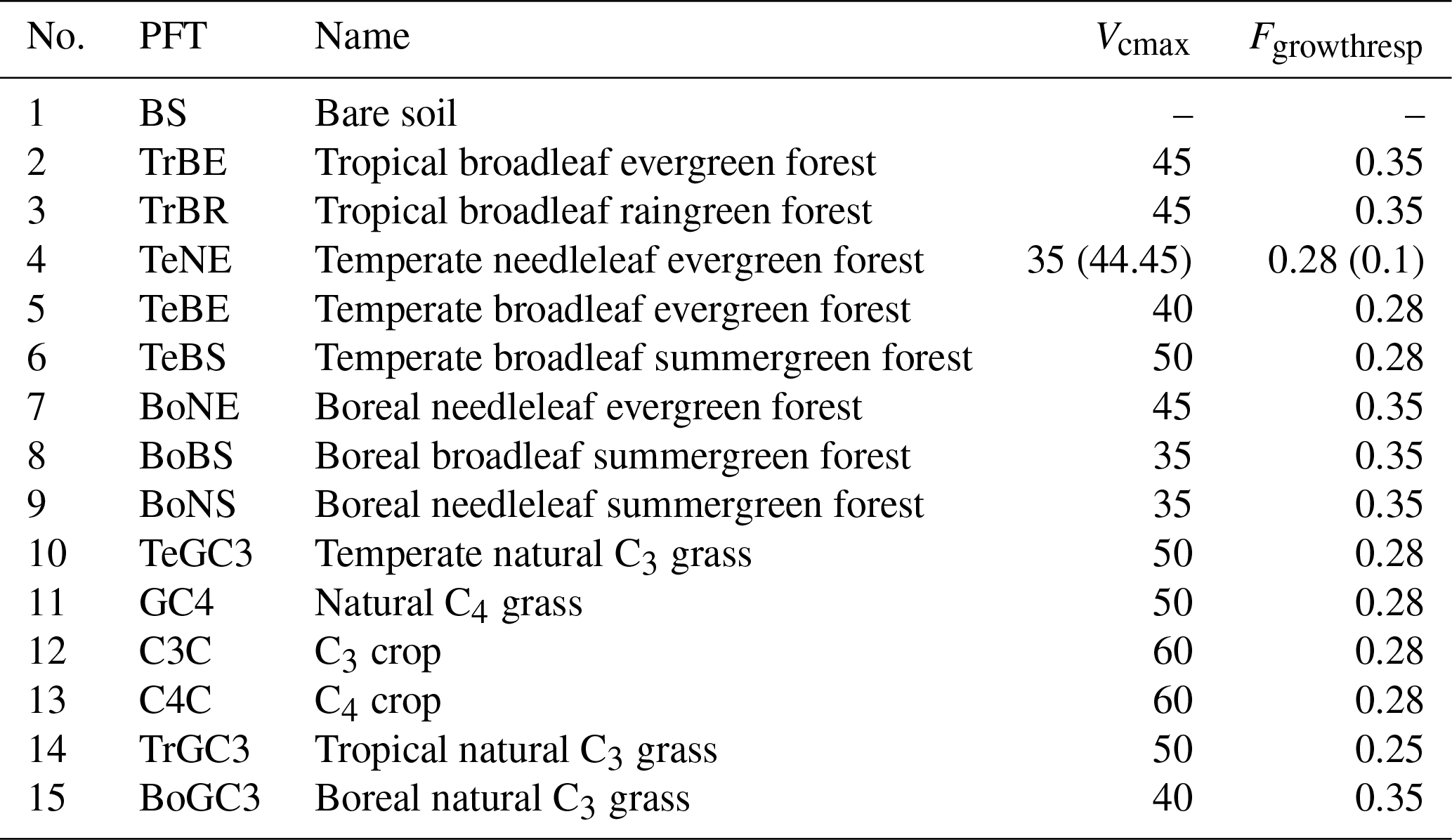
ORCHIDEE version 2.2 is a state-of-the-art DGVM designed to simulate carbon, water, and energy fluxes from local sites to the global level (Krinner et al., 2005). It calculates the energy and hydrology budget of the terrestrial biosphere at half-hourly intervals, distinguishing 15 plant functional types (PFTs; shown in Table 1) (Ducoudré et al., 1993; de Rosnay and Polcher, 1998). In addition, it simulates vegetation phenology and carbon dynamics, including photosynthesis, maintenance and growth respiration, carbon allocation in vegetation biomass, production and decomposition of litter, and soil carbon dynamics, at daily time steps (Krinner et al., 2005). The basic scheme of biospheric carbon cycling representation in ORCHIDEE is described in Appendix A.

ORCHIDEE is forced with meteorological data, wood harvest maps, soil texture, and land cover maps to prescribe the areal proportion of each PFT in each model grid cell for a given point in time. When land cover changes happen, PFT-level carbon stocks are redistributed from the shrinking PFT to the expanding one.

All simulations described in this study share the same forcing data. In detail, we employed the Climatic Research Unit and Japanese Reanalysis (CRU JRA) v2.3 dataset for meteorological forcings with a spatial resolution of 0.5°. This dataset is accessible for the period spanning 1901 to 2021 and is available at https://catalogue.ceda.ac.uk/uuid/38715b12b22043118a208acd61771917 (last access: 15 May 2023). The CRU JRA v2.3 data comprise 6-hourly records of various variables, including temperature at 2 m above ground, air pressure, specific humidity, wind speed, precipitation (rain and snow), and downward longwave and shortwave radiation. The land cover map is from the European Space Agency (ESA) LUH2v2 data (Lurton et al., 2020), i.e. a combination of the ESA Climate Change Initiative land cover map (https://www.esa-landcover-cci.org/, last access: 15 May 2023) and the historical land-use harmonisation database (LUH2v2; Hurtt et al., 2020). These data provide areal fractions for each of the 15 PFTs within individual cells of the modelling grid. The land cover map is updated annually, and LUC is represented as an abrupt transition of land cover at the beginning of each year. More subtle LUC changes, like changes in management intensity, are not considered due to a lack of historical data. Over standard historical gridded simulations, LUC change is treated as a continuous process, slightly increasing or decreasing the areal proportion of one or more PFTs at the detriment of others. The litter and SOC pools inherited from a disappearing PFT to a target PFT are merged with the existing litter and SOC pools of the target PFT, which already occupy a fraction of the grid cell. This dilution of a small amount of newly delivered litter and SOC brought from LUC into a large amount of SOC already existing in the target PFT area conserves mass but makes it impractical to compare SOC and litter change with observations because observations come from sites where 100 % of a PFT is converted to another.

Therefore, we built idealised LUC scenarios in which we assume an abrupt transition referring to a 100 % conversion from one PFT to another in a grid, meaning there is no dilution of old soil carbon signals into the new PFT area. This transition is based on homogeneously prescribed land cover consisting of one single PFT, not on changing land cover maps. This abrupt change run is necessary to make simulations comparable to observations at the site level, which consider local change from one PFT to another rather than a change in PFT mix from the landscape perspective usually taken by a DGVM such as ORCHIDEE. The wood harvest map is sourced from the LUH2v2 database. It provides the wood harvest data as annual areal flux rates of carbon in the extracted biomass (gC m⁻² yr⁻¹). This means that these data can be applied to different PFT maps without causing extreme flux rates due to inconsistent representation of forest area. The soil texture classification relies on the study of Post and Zobler (2000). This scheme distinguishes seven texture classes, which for ORCHIDEE are further aggregated into three texture classes (i.e. coarse, medium, fine), each associated with specific soil physical properties. This classification is essential for simulating the soil water budget, and through that, it also significantly affects vegetation dynamics. In addition, it impacts soil carbon dynamics by directly influencing the turnover rates of SOC through clay content and its presumed effect of enhancing the physical protection of the active SOC pool. In ORCHIDEE, the module of soil has an assumed globally uniform depth of 2 m. Note however that soil carbon is not depth discretised, and average values of soil temperature, moisture, and clay content are used.

Table 1 ORCHIDEE plant functional types (PFTs) and PFT-specific parameters. Values in parentheses indicate the modifications in the simulation set-ups (detailed in Sect. 2.3). (V_cmax represents the maximal rate of carboxylation (≈ the potential photosynthetic capacity) (µmol m⁻² s⁻¹); F_growthresp is the fraction of gross primary production (GPP) which is lost as growth respiration.)

2.2 Observation-based data

To evaluate the model's performance concerning the dynamics of carbon stocks, we compare simulation results against observations of net primary production (NPP) and gross primary production (GPP), which are the primary factors controlling land carbon stocks; paired observations of above-ground biomass and plant age (Somogyi et al., 2008; Schepaschenko et al., 2017); observation-based maps of SOC; and SOC stock changes due to LUC. For the investigation of potential factors (detailed in Sect. 2.2.4) causing model bias in estimating changes in SOC stocks due to LUC, we used meteorological data from the CRU JRA dataset and soil-related data from Land Use and Cover Area frame Survey (LUCAS) soil surveys.

2.2.1 Primary production

Annual NPP data were derived from a comprehensive forest ecosystem database from Luyssaert et al. (2007), including a rigorous selection of single or multiple direct measurements and modelled fluxes. The model-generated fluxes in this database closely match the observed data because they were generated using a mechanistic process model with daily or more detailed climatological data, calibrated with site-specific parameters, and validated against site-specific measurements. NPP is reported at different levels, ranging from a single plant component (e.g. foliage or stem NPPs) to the complete plant. Here, we selected the most superficial aggregation level of the total NPP (i.e. the sum of above-ground (foliage + wood) and below-ground (coarse + fine roots) NPP components).

The observed annual GPP data were obtained from four datasets. The first dataset was, similar to the above NPP dataset, extracted from the global forest database from Luyssaert et al. (2007). Second, GPP data were also gathered from the FLUXNET 2015 dataset, including data from multiple regional flux networks (Pastorello et al., 2020). This dataset collects eddy covariance measurements of carbon, water, and energy fluxes between the biosphere and atmosphere. It can be downloaded from https://fluxnet.org/data/fluxnet2015-dataset/ (Pastorello et al., 2020). Over our study area, these GPP data are available mainly from 1996 to 2015. Thirdly, additional GPP data from European sites in 2020 were collected from the Integrated Carbon Observation System (ICOS), a European-wide greenhouse gas research infrastructure. Finally, GPP data were also gathered from Campioli et al. (2015). Like the comprehensive database of Luyssaert et al. (2007), Campioli et al. (2015) compiled the data from individual studies using harvest, biometric, eddy covariance, or process-based model estimates of primary production. In addition, this dataset includes data not only from forest sites but also from grassland and cropland sites.

More detailed information on the selected NPP and GPP sites from different sources can be found in the Supplement (Tables S1 to S4).

2.2.2 Biomass

The biomass dataset considered here includes in situ estimates for the different plant compartments (i.e. foliage, stem, and branch) and spans all of the European biomes (Fig. S1 in the Supplement). The dataset consists of a collection and harmonisation of available open forest inventory databases (e.g. Somogyi et al., 2008; Schepaschenko et al., 2017; Anderson-Teixeira et al., 2018) already used to quantify ecological and environmental controls on the spatial variability of stand age (Besnard et al., 2021). Despite the global nature of the dataset, given the current European scope of this analysis, here we focused on locations in Europe where the total above-ground biomass (AGB) could be estimated based on in situ measurements. The final dataset comprises 603 sites, including six PFTs (TeNE, TeBS, BoNE, BoBS, and a few sites of TeBE and BoNS). The average stand age is 58 years (with a standard deviation of 43), and the mean AGB is 6.4 kgC m⁻² (with a standard deviation of 4.5).

2.2.3 Soil organic carbon

Data on SOC stocks were obtained from the Land Use and Cover Area frame Survey (LUCAS) collected during 2018 (Orgiazzi et al., 2018). This dataset offers comprehensive information on various chemical and physical soil properties throughout the European region. The LUCAS sampling was conducted at different depths, primarily focusing on the fine-soil component of the top 20 cm of the soil column while excluding above-ground vegetation residues, grass, and litter. Site selection for our study was based on the availability of observed organic carbon content, bulk density, and the fraction of coarse fragments within the top 20 cm layer. In addition, the land-use information was consistently available for all samples.

We considered the latest surveys from LUCAS 2018 topsoil data (Fernandez-Ugalde et al., 2022), which can be downloaded from the European Soil Data Centre's website https://esdac.jrc.ec.europa.eu/content/lucas-2018-topsoil-data. However, it is important to note that, at the time of writing this paper, the fraction of coarse fragments was not included in the LUCAS 2018 topsoil data and had to be obtained from a previous survey, LUCAS 2015 (Jones et al., 2020). We downloaded and extracted the coarse-fragment data from https://esdac.jrc.ec.europa.eu/content/lucas2015-topsoil-data (last access: 3 August 2023) and then combined them with the LUCAS 2018 topsoil data. Furthermore, our analysis focused only on samples associated with forest, grassland, and cropland land uses, excluding other land-use types not represented by the PFTs of ORCHIDEE, such as shrubland or wetlands. In total, we identified and included 5150 sampling sites in our study.

The total SOC (in kg m⁻²) stocks were then calculated based on the following equation (Batjes, 1996):

$$\begin{array}{}\text{(1)}& \mathrm{SOC}={\displaystyle \frac{\mathrm{OC}\times \mathrm{BD}\times D\times (\mathrm{1}-\mathrm{CF})}{\mathrm{100}}},\end{array}$$

in which OC is organic carbon content (gC kg⁻¹), BD is bulk density (gC cm⁻³), D is soil depth (cm), and CF is the volumetric fraction of coarse fragments (>2 mm).

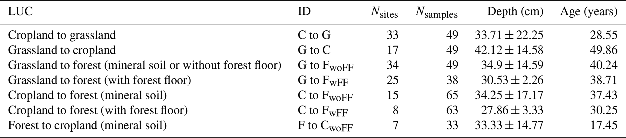
We compiled data from 102 study sites sourced from 34 peer-reviewed publications (detailed in Table S5 in the Supplement) investigating the impact of LUC on soil carbon stocks in the European region. Our selection process included several criteria to identify relevant SOC data from these studies. Firstly, we focused on five specific LUC transitions: cropland to grassland (C to G), grassland to cropland (G to C), cropland to forest (C to F), grassland to forest (G to F), and forest to cropland (F to C). Secondly, we included only studies with paired plots, chronosequences, or repeated sampling designs. Paired plots involve assessing two adjacent sites – one that has not experienced LUC and has the original land cover and the other with a new land cover after LUC. Similarly, chronosequences utilise adjacent plots with different ages of new vegetation since conversion to another land-use type. Repeated or mono-site sampling involves the periodic collection of soil samples at the same location/site. A “space-for-time” approach, assuming that the SOC stocks of prior land use are in a steady state, is used in paired plots and chronosequences. Thirdly, we required information about whether the forest floor (i.e. the above-ground litter organic layer) was included in the sampling process for forest sites. Finally, additional relevant properties such as sampling depth, land-use history, age of current land use, and the unit of soil carbon stocks must be provided. The collected data were finally categorised into seven conversion types, as detailed in Table 2.

Table 2 Number of study sites and samples, mean sampling depths with standard deviation, and mean current land-use age for the local-scale observations in the meta-analyses.

2.2.4 Additional data for model bias attribution

We considered two important meteorological variables, the air temperature at 2 m a.g.l. and precipitation, which are derived from the Climatic Research Unit and Japanese Reanalysis (CRU JRA) v2.3 dataset. This dataset is also used for the meteorological forcings in ORCHIDEE and is detailed in the next section (Sect. 2.3).

Soil-related data are obtained from Ballabio et al. (2019), who provided maps of soil chemical properties at 500 m spatial resolution across Europe using soil point data from LUCAS 2009/2012 soil surveys (Toth et al., 2013). These datasets align with the observed SOC stocks (see Sect. 2.2.3) and are considered among the most reliable data sources for Europe (d'Andrimont et al., 2020). Our focus was on three key properties: the soil carbon-to-nitrogen (CN) ratio, nitrogen (N), and phosphorus (P). The data were retrieved from https://esdac.jrc.ec.europa.eu/content/chemical-properties-european-scale-based-lucas-topsoil-data (last access: 3 August 2023). Additionally, our study considered the annual soil erosion rate in 2009 (Fendrich et al., 2022; available at https://esdac.jrc.ec.europa.eu/themes/historical-reconstruction-erosion, last access: 3 August 2023), which we considered to be representative of the last few decades. The maps of all soil-related data are aggregated to 0.5° grids to match ORCHIDEE's resolution.

2.3 ORCHIDEE simulations

We conducted simulations with the ORCHIDEE model across Europe (33 to 70° N and 10° W to 40° E) for a straightforward comparison to observational data (Table 3). These simulations can be categorised into two groups: (a) realistic simulations for the historic period aimed at evaluating the ORCHIDEE model's ability to reproduce observed primary production (NPP, GPP), biomass carbon stocks, and SOC stocks and (b) idealised LUC simulations aimed at evaluating the biomass carbon stock changes and the effects of LUC on SOC stocks in terms of total magnitude and timing.

2.3.1 Historical simulations

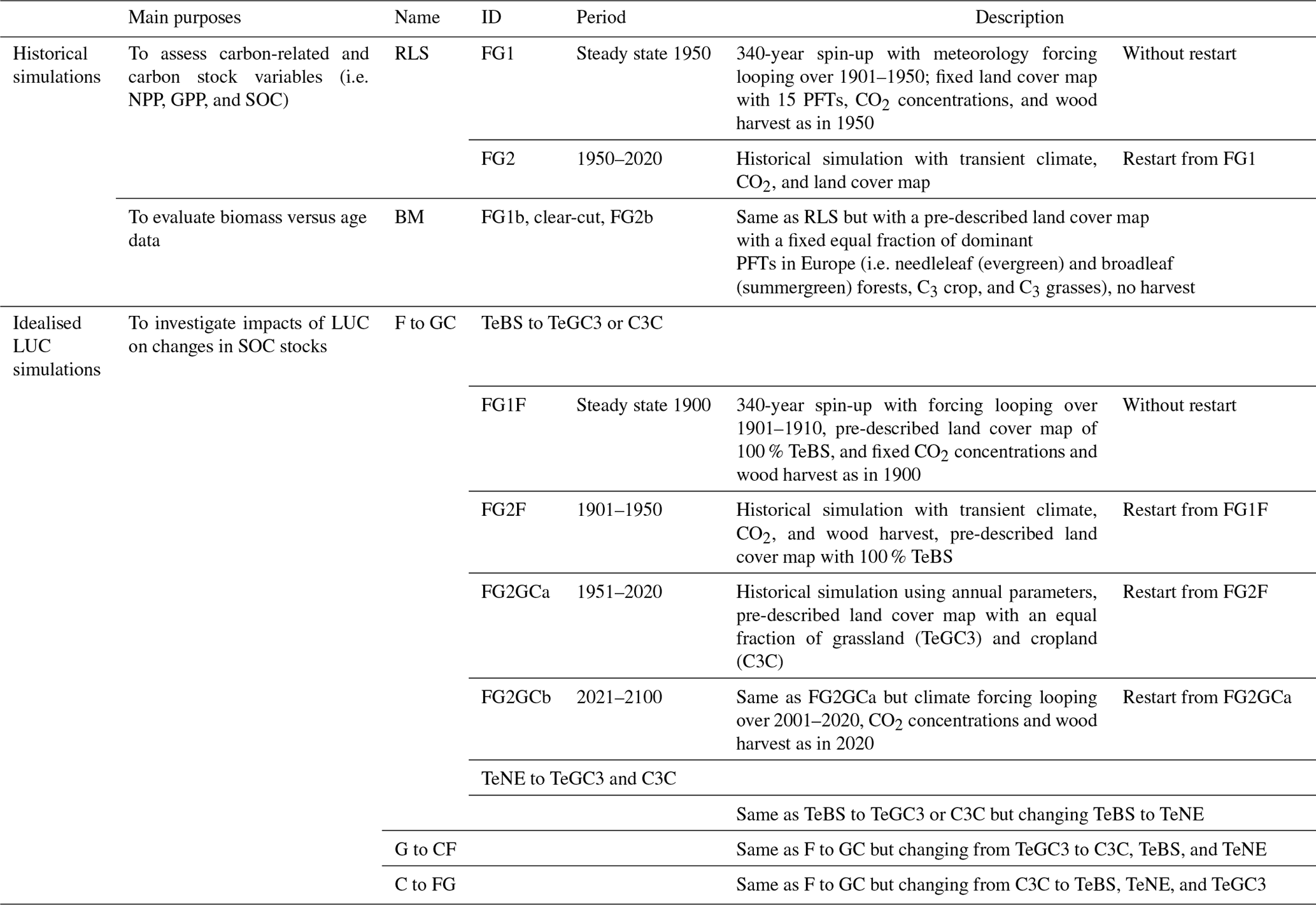
Firstly, the realistic simulation, referred to as RLS, is based on the default configuration and parameters inspired by the TRENDY protocol (Sitch et al., 2015), including two steps. In the first step of our simulations (FG1), we spun up the model to reach a steady state representative of the year 1950. This involved conducting a simulation over 340 years, with a 30-year loop of meteorological forcing data (1921–1950), as well as fixed values for atmospheric CO₂ levels, PFT maps, and wood harvest, all corresponding to the year 1950. The PFT map employed here consists of 15 PFTs (Boucher et al., 2020), as specified in Table 1. In the second step, we ran a transient simulation (FG2) from 1950 to 2020 using historical meteorology, CO₂ concentrations, and wood harvest data. The FG2 was restarted from the last year of output of FG1. These RLS simulation outputs are evaluated against the observation-driven NPP, GPP, and SOC data, as detailed in Sect. 2.4.

Secondly, we performed a BM simulation (where BM refers to biomass assessment), which uses the same configuration as RLS but pre-describing the land cover with constant fractions of dominant PFTs in the EU (see Table 1) and no wood harvest, which ensures PFT carbon stocks for the observation period are not affected by LUC for the comparison with the observation of natural forest. In addition, a forest clear-cut simulation is performed before running the transient simulation, and during FG2 the biomass regrows from approximately zero. Thus, the simulated forest age was defined as the time since the beginning of the FG2 simulation.

Furthermore, in all simulations, we calibrated, by trial and error, two parameters, namely V_cmax and F_growthresp, specifically for the temperate needleleaf evergreen forest (TeNE) to reduce biases in NPP, GPP, and AGB (see more in Sect. 3.1 and 3.2). Our initial objective was to approximate the correct values of NPP and GPP, ultimately leading to an improved representation of AGB. In detail, V_cmax is adjusted based on the observed-to-simulated GPP ratio, and F_growthresp is gradually reduced to increase NPP and GPP values to be closer to the observations. The final adjusted values for these parameters are indicated in parentheses in Table 1.

2.3.2 Idealised LUC simulations

We conducted idealised LUC simulations, assuming the entire study area was covered by a single PFT. To ensure accurate comparisons between simulated results and meta-analyses from site-level carbon pool changes caused by LUC, regions where this PFT does not occur according to the PFT maps were excluded from the analysis. Then, we transformed this initial PFT into other PFTs, such as temperate broadleaf summergreen forest to temperate natural C₃ grassland and C₃ cropland (TeBS to TeGC3 or C3C, aberrations as presented in Table 1). These transformations exemplify the conversion of forest areas into grasslands or croplands (referred to as F-to-GC conversion). Note that ORCHIDEE simulates SOC stocks separately for each PFT, allowing us to simultaneously represent LUC from one PFT to two different PFTs. This is an improvement compared to other DGVMs that typically assign one value of SOC to all PFTs (e.g. the LPJ model, Sitch et al., 2003).

The LUC simulations are somewhat similar to the RLS simulation, including two main processes, i.e. the spin-up simulation FG1 and the transient historical simulation FG2. In detail, we first ran the 340-year spin-up FG1F looping over 10 years of meteorological forcing (1901–1910) and fixed atmospheric CO₂ concentrations and wood harvest as in 1900 in the F-to-GC simulation. Here, we fixed land cover to 100 % TeBS. At this stage, the biomass and SOC stocks are in equilibrium. In the second step, we ran a historical simulation FG2F from 1901 to 1950 for this same PFT (with historical meteorology, CO₂ concentrations, and wood harvest data), restarting from the last year of the spin-up simulation FG1F. To perform the LUCs (in this case, from F to G and F to C), we changed the prescribed PFTs to C₃ grassland and cropland (i.e. TeGC3 and C3C) and continued running the historical simulation FG2GCa from 1951 to 2020, restarting from FG2F. In addition, to study the LUC impact for a longer period, we extended the model run until 2100, looping over the last 20 years of meteorological forcing data (2001–2020). For this extended simulation, we kept the atmospheric CO₂ fixed to the value in 2020. Although the projected climate is available (e.g. data from the Coupled Model Intercomparison Project Phase 6, Eyring et al., 2016), historical data were used here to be compatible with the meta-analyses. Other LUC simulations, i.e. G to CF and C to FG, were set up similarly.

We acknowledge that defining 1950 as the same year of LUC in our simulations increases the uncertainties when comparing simulations to observations which relate to different years of LUC. Note that only a fraction of the studies from which we source the observed LUC impacts on SOC stocks specifies the year of LUC. To explore this source of uncertainty, we thus conducted tailored simulations matching the individual years of LUC reported in these studies and compared the results to simulations using 1950 as the year of LUC. Detailed information about these additional simulations is provided and discussed in Sect. S1 of the Supplement.

Table 3 Main simulations.

2.4 Model–data comparisons

Our ORCHIDEE simulations generate outputs encompassing all grid cells at a resolution of 0.5° (≈50 km) over Europe. Conversely, observational data are typically collected at specific locations. To facilitate the comparison between the observed and simulated values, each observational site was matched with the closest corresponding ORCHIDEE cell. This approach ensures a comprehensive evaluation of the model's performance in relation to the observed data.

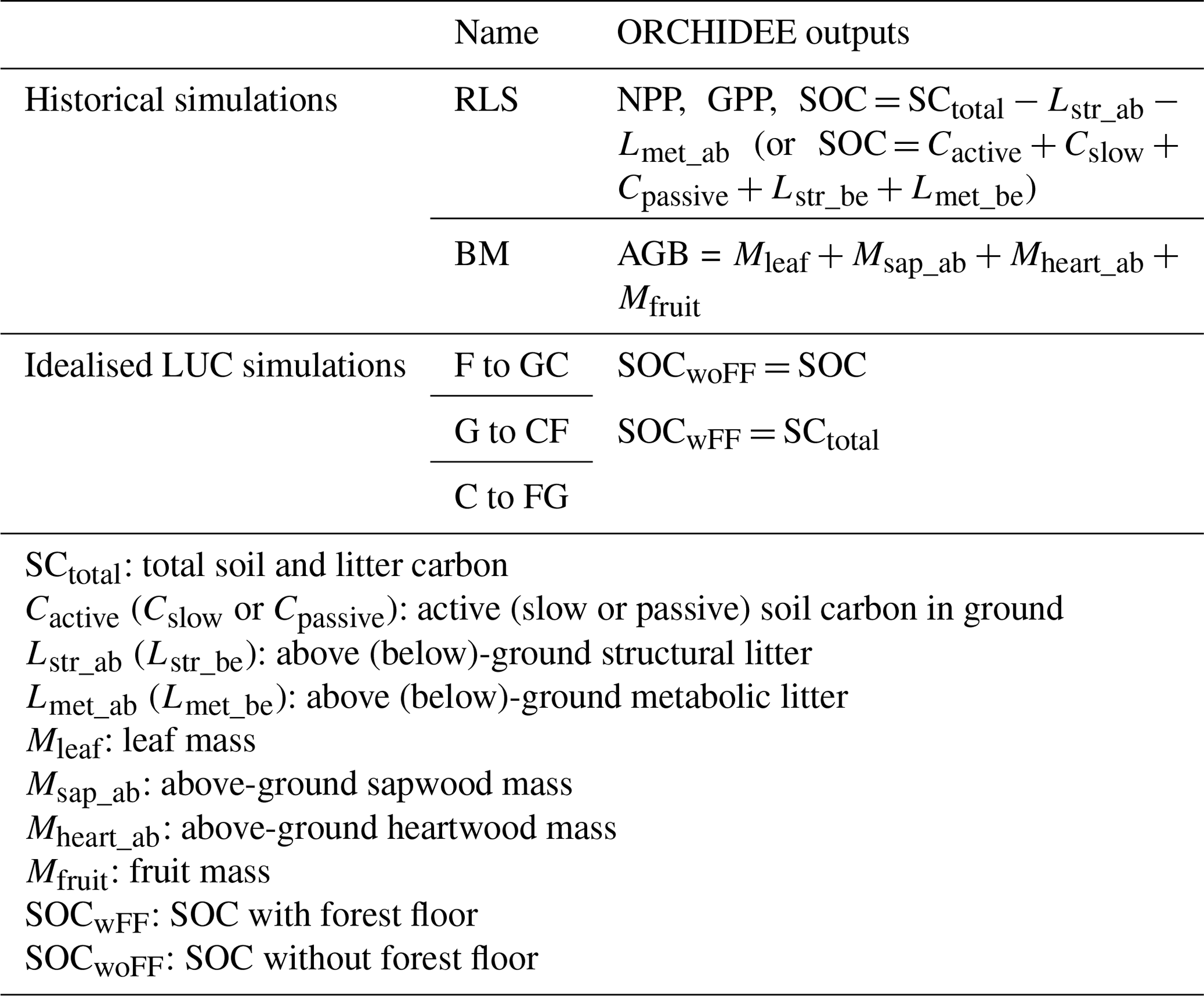
Table 4 Model outputs corresponding to the simulations in Table 3.

2.4.1 Historical simulations

To compare simulated NPP and GPP against observations, we used NPP and GPP outputs from the FG2 RLS simulation for the respective observed years and corresponding PFTs. In cases where the PFT was absent or unclear in the observations (e.g. mixed forest), we assigned the dominant PFT in that particular site based on the ESA LUH2v2 land cover map. We then grouped the observed and simulated values by PFT and employed boxplots for comparison. The boxplot representation offers valuable insights into the statistical distribution of values, including the median, the 25th and 75th percentiles, the range of extreme data points, and any outliers.

Similarly, we used boxplot representation to evaluate AGB simulations categorised by PFT and age groups. The age groups are divided as follows: group 1 – 0 to 19 years, group 2 – 20 to 39 years, group 3 – 40 to 59 years, group 4 – 60 to 79 years, group 5 – 80 to 99 years, and group 6 – >99 years. ORCHIDEE simulates biomass for different plant compartments (e.g. leaves, wood, roots). To maintain consistency with the observations, simulated AGB was derived from the BM simulation by summing the biomass of leaves, above-ground sapwood and heartwood, and fruits.

We used three diagnostic measures to assess ORCHIDEE's performance in simulating soil carbon stocks (i.e. the FG2 RLS simulation's outputs). These measures include Pearson's correlation (COR; unitless), root mean square error (RMSE; in kg m⁻²), and relative RMSE (rRMSE; in %) between the observed and simulated SOC. The above-ground litter was excluded from the simulated SOC for comparison to the LUCAS data. The calculation of ORCHIDEE's outputs is detailed in Table 4.

2.4.2 Idealised LUC simulations

Soil profile data in meta-analyses are reported at various depths (as detailed in Table 2). To ensure uniform comparisons, we first standardised all soil carbon data, both observed and simulated, to represent SOC stocks in the top 30 cm, utilising the following depth function (Jobbágy and Jackson, 2000; Deng et al., 2016):

$$\begin{array}{}\text{(2)}& {\displaystyle }{X}_{\mathrm{30}}={\displaystyle \frac{\mathrm{1}-{\mathit{\beta }}^{\mathrm{30}}}{\mathrm{1}-{\mathit{\beta }}^{d\mathrm{0}}}}\times X_{d\mathrm{0}},\end{array}$$

where X₃₀ represents the soil carbon stocks in the top 30 cm, d0 is the original soil depth available in observations or simulations (in cm), X_d0 is the original soil carbon stocks, and β characterises relative rates of decrease with depth (β=0.9786, unitless). For instance, a simulated sample X_ORC at 2 m depth (d0=200) is converted into the topsoil sample using the equation $X_{\mathrm{30}}=\frac{\mathrm{1}-{\mathrm{0.9786}}^{\mathrm{30}}}{\mathrm{1}-{\mathrm{0.9786}}^{\mathrm{200}}}\times X_{\mathrm{ORC}}=\mathrm{0.48}\times X_{\mathrm{ORC}}$.

We then used the absolute SOC stock change (ΔSOC; in kg m⁻²) as a variable for the comparison of soil carbon changes:

$$\begin{array}{}\text{(3)}& \mathrm{\Delta }\mathrm{SOC}={\mathrm{SOC}}_{\mathrm{LU}\mathrm{2}}-{\mathrm{SOC}}_{\mathrm{LU}\mathrm{1}},\end{array}$$

where LU1 corresponds to the land use before conversion, and LU2 is the land use after conversion. Similar to the observations, the simulated SOC for the prior land use is assumed to be in a steady state. For example, in the conversion from F to GC, the simulated SOC_LU1 is set to be equal to the SOC value in 1950 from the FG2F simulation (Table 3). In contrast, the observed SOC measurements after land cover conversion are taken at various ages. A fitted carbon response function (CRF), detailed below, is derived for each conversion, describing the ΔSOC as a function of time. For the simulations, a distinct response function was derived from the simulation, corresponding to each meta-analyses site. Subsequently, the average simulated soil carbon response was computed across all these response functions. This aggregate response, referred to as “simulated CRF”, was then compared with the fitted or observed CRF obtained from the meta-analyses.

The observed CRF was constructed using diverse regression models, including linear regression, second- and third-order polynomial regressions, and single-term and two-term exponential models. Due to the limited size of the observed samples (as detailed in Table 2), a leave-one-out cross-validation (LOOCV) method (Stone, 1974; Dinh and Aires, 2022) was employed for the model selection process. This iterative approach facilitates the validation of each model's performance by training it on all data points but one and evaluating its prediction accuracy on the excluded data point. By repeating this process for all data points and assessing the overall performance, we can identify the best-performing model that generalises well to the entire dataset and the new samples. Finally, the models providing the most adequate description of the temporal dynamic of relative SOC stock changes were the linear function (Eq. 4) and the single-term exponential function (Eq. 5):

$$\begin{array}{}\text{(4)}& {\displaystyle }\mathrm{\Delta }\mathrm{SOC}=at+b,\text{(5)}& {\displaystyle }\mathrm{\Delta }\mathrm{SOC}=a\times e^{b*t},\end{array}$$

where t is the time after LUC (years), and a and b are regression coefficients. A detailed fitted CRF for each LUC in meta-analyses is presented in Table S6 in the Supplement. Furthermore, to better understand the accuracy and uncertainty of the fitted CRFs, we established approximate 95 % confidence intervals using simultaneous prediction bounds for the fitted functions. These confidence intervals visually represent the range of potential outcomes, providing valuable insights into the variability of the observed carbon stock change rate.

2.4.3 Factors explaining model bias

We used random forest (RF) (Breiman, 2001; Liaw and Wiener, 2002) to explore the factors contributing to bias in estimating SOC stock changes following LUC. The bias is calculated for each site observation taken from the meta-analyses (Table 2). For this, we compared the observed SOC stock changes per site with corresponding simulated values from the corresponding ORCHIDEE grid cells. Then we analysed which predictor variables best explain the site-to-site variations in model bias for each LUC scenario. Our chosen explanatory variables encompassed both meteorological variables (i.e. temperature at 2 m a.g.l. (T2m) and rainfall (Rain)) and key soil-related metrics (i.e. soil carbon-to-nitrogen ratio (CN), nitrogen (N), phosphorus (P), and soil erosion rate (ER)). Given the constraints of the available observations (Table 2), we also employed LOOCV here to assess the performance of the RF regression model for each LUC scenario. The model consists of 100 decision trees. Each tree is constructed independently and operates on a random subset of the data. During the LOOCV process, the model iterates through each sample in the dataset, systematically excluding one for validation in each iteration. Subsequently, the model is trained on the remaining samples, and feature importance is cumulatively assessed throughout each iteration. The performance of this LOOCV process is shown in Table S7 in the Supplement. The LUC scenarios with poor RF regression results are excluded. For the remaining cases, we then derived importance scores (Liaw and Wiener, 2002) associated with individual explanatory variables. These scores are then normalised or scaled from 0 to 1, with a value of 1 denoting the utmost relevance and 0 signifying the lowest relevance concerning the model bias.

3 The performance of the ORCHIDEE model

3.1 Net and gross primary productivity (NPP and GPP)

Figure 1 compares the simulated NPP and GPP values with site observations (Sect. 2.2.1). Both simulations and observations exhibit comparable ranges across various PFTs, notably showcasing good performance in temperate forests and temperate C₃ grasslands, where the relative differences in the medians are around 10 %. However, the ORCHIDEE simulation results often present a narrower range than the observed site data. This difference can be attributed to the fact that the ORCHIDEE PFTs are a rigid classification of vegetation, with each PFT representing the average characteristics of various tree species. In contrast, differences between individual species within the same PFT class can be substantial (Poulter et al., 2011). On the contrary, observations refer to individual species.

The calibration of V_cmax and F_growthresp parameters for TeNE (see Table 1) resulted in considerable improvement, in particular for NPP. The default parameterisation (V_cmax=35 and F_growthresp=0.28) resulted in the simulated NPP median deviating by approximately 32 % from the observed value. The adjusted parameters (V_cmax=44.45 and F_growthresp=0.1) reduced deviation to 5 %.

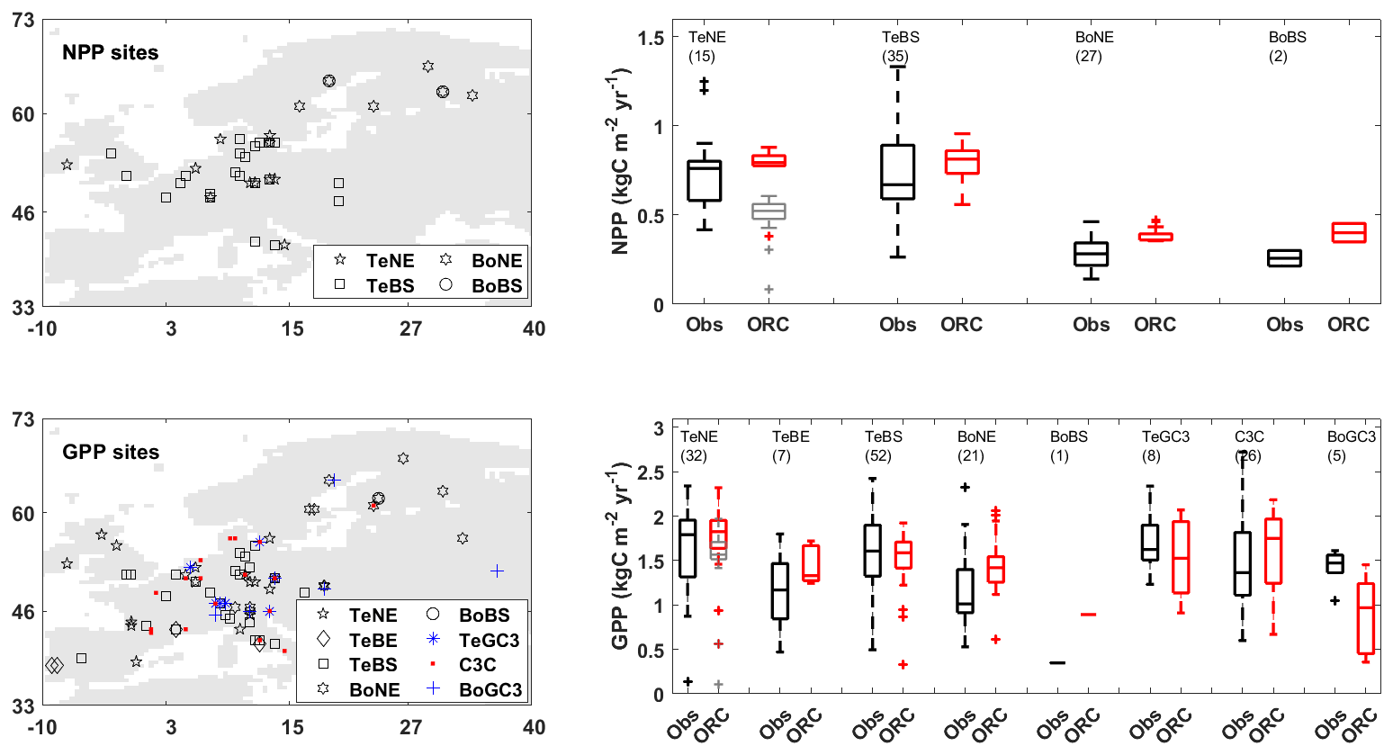
Figure 1 Maps of net and gross primary productivity (NPP and GPP) sites, along with boxplots comparing observations (Obs in black) and ORCHIDEE (ORC in red) simulations. The grey boxes show outputs from ORCHIDEE's default configuration (i.e. without calibrating V_cmax and F_growthresp parameters) for comparison purposes. In each boxplot, the number in parentheses indicates the number of sites in each plant functional type (PFT) group.

3.2 Above-ground biomass (AGB)

The boxplots in Fig. 2 present AGB versus age comparisons between observations (in black) and simulations (in red) for four PFTs (TeNE, TeBS, BoNE, and BoBS) and each age group. Other types of forest PFTs were excluded due to the limited number of observed samples. Simulations capture the same trend as the observations: AGB increases quickly in young stands (i.e. <60 years old) and moderately saturates at later ages (>60 years old). Like the NPP and GPP comparisons, the observed AGBs appear in more extensive ranges and have more extremes than the simulated values for all considered PFTs.

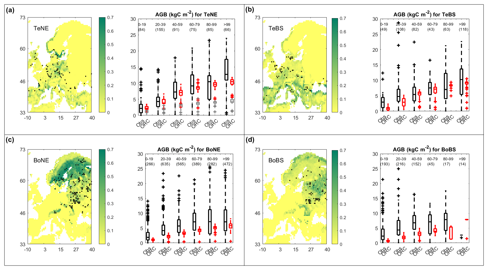
Figure 2 Maps of above-ground biomass (AGB) sites for four plant functional types (PFTs), including temperate needleleaf and broadleaf, as well as boreal needleleaf and broadleaf forests (TeNE, TeBS, BoNE, BoBS), along with boxplots comparing observations (Obs in black) and ORCHIDEE (ORC in red) simulations. In the boxplot of the TeNE forest (a), the grey boxes present outputs from ORCHIDEE's default configuration (i.e. without calibrating V_cmax and F_growthresp parameters), for comparison purposes. In each boxplot, the number in parentheses indicates the number of sites in each age group (group 1: 0–19 years, group 2: 20–39 years, group 3: 40–59 years, group 4: 60–79 years, group 5: 80–99 years, group 6: >99 years). The colour scale in the maps indicates the ORCHIDEE vegetation fraction.

Again, the adjustment of V_cmax and F_growthresp parameters for TeNE (see Table 1) improved the simulated AGB age curves significantly, while in the original set-up, the simulated values are much lower compared to the observed ones. This improvement is visually represented in the boxplot of the TeNE forest, in Fig. 2a: the grey boxes, representing AGB values obtained from the default settings, indicate a median deviation of about 60 % from the observed values (black boxes) across five age groups. Conversely, with our calibration, this deviation is reduced to less than 10 %, as indicated by the red boxes, which now closely align with the observed data represented by the black boxes.

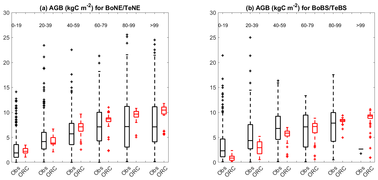
Figure 3 The same as the boxplots in Fig. 2 but for the comparison of the observed values for the BoNE forest with simulated values for the TeNE forest (a), as well as observed values for the BoBS forest with simulated values for the TeBS forest (b).

Furthermore, Fig. 2 highlights a contrast in ORCHIDEE performance; notably, boreal forests exhibit lower biomass per age class than temperate ones, illustrated by BoNE versus TeNE and BoBS versus TeBS forests. Interestingly, observed biomass ranges for BoNE and BoBS forests closely resemble those of TeNE and TeBS forests. Further comparisons are detailed in Fig. 3, despite variations in site numbers between observations and simulations for each age group. This comparative approach provides insights into and offers a broader understanding of how the model's parameterisation performs in Europe. We found that the parameterisation of BoNE and BoBS may need improvement, as they appear less well fitted than TeNE and TeBS. This might raise questions about the relevance and necessity of using BoNE and BoBS as distinct PFTs when TeNE and TeBS demonstrate better alignment with the observed data in the study region.

3.3 Soil organic carbon (SOC)

The SOC map showing 5150 LUCAS samples is presented in Fig. 4a. We also generated a corresponding SOC map using the ORCHIDEE simulation weighted by the areal proportions of each PFT. The difference between our simulated SOC stocks from LUCAS data is presented in Fig. 4b. The correlation between the observed and simulated SOCs is 0.4 (and RMSE = 2.03 kg m⁻², rRMSE = 50.31 %), indicating moderate agreement. However, it is essential to note that this general ORCHIDEE simulation does not represent peatlands or important factors such as land management, effects of soil erosion and translocation of SOC from eroded sides to colluvial sediments, topographic wetness, land-use history before 1900, soil class, and geochemistry of soil-forming substrates, etc. Therefore, achieving a correlation coefficient of 0.4 is already significant. Notably, ORCHIDEE underestimates SOC in certain regions, particularly in northern Europe. This discrepancy can be explained by the absence of peatlands in this particular version of ORCHIDEE.

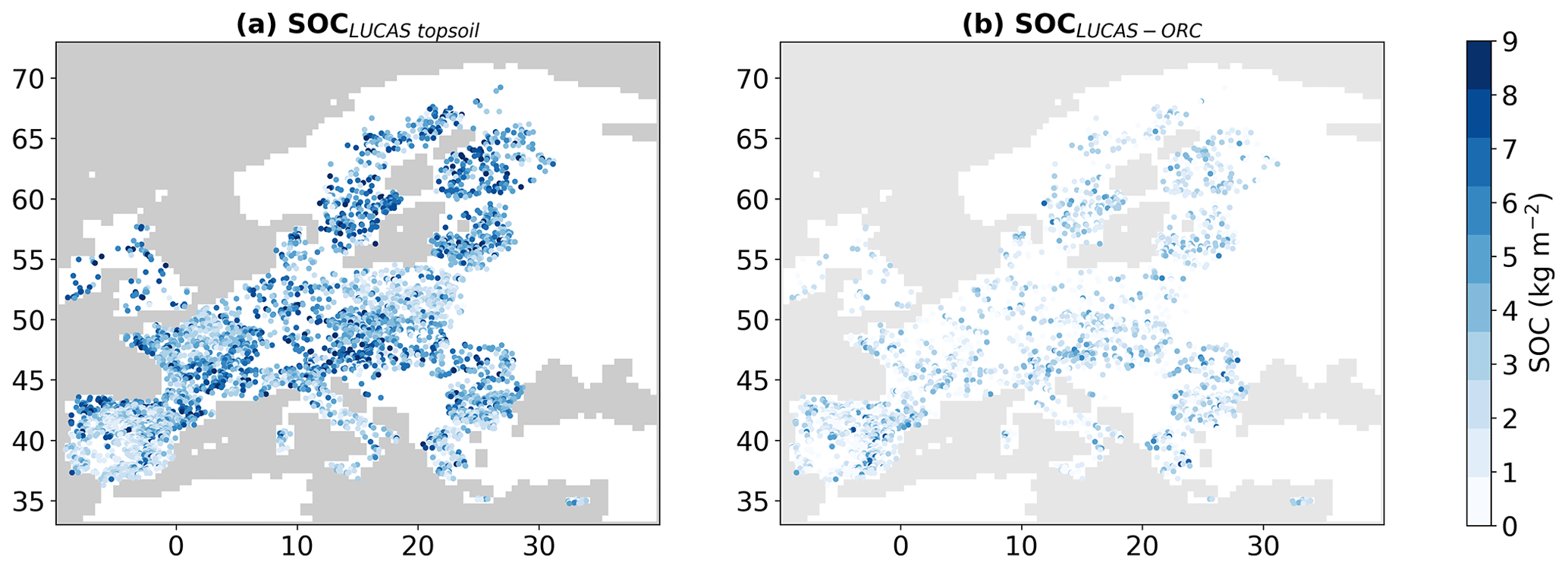
Figure 4 Maps showing the stocks after soil organic carbon (SOC in kg m⁻²) based on the LUCAS topsoil database (a) and the deviation of simulated SOC stocks from these observation-based estimates (b).

In the following, we classified 5150 SOC samples into three vegetation groups (forest, grass, and crop) based on the land-use information provided in the LUCAS dataset. The assessment of observed and simulated SOC stocks is illustrated through comparison scores (COR, RMSE, and rRMSE) in Table S8 within the Supplement, along with scatterplots and histograms in Fig. 5, showcasing variations across different grid scales: 0.5° × 0.5°, 1° × 1°, 2° × 2°, and 3° × 3° cells. This stepwise aggregation aims to enhance our understanding of how far spatial correlations between observed and modelled SOC stocks are scale dependent. At the 0.5° × 0.5° scale, the correlation between observed and simulated SOC for forest sites (Fig. 5a1) is relatively low (COR = 0.17, rRMSE = 59.15 %). However, the correlation values are significantly better for grassland and cropland sites (Fig. 5b1 and c1), reaching 0.53 and 0.42, respectively (with corresponding rRMSE values of 39.38 % and 35.98 %). Interestingly, the correlation scores improve for all vegetation types as we increase the grid-scale size and, thus, the level of spatial aggregation. For example, when examining the 3° × 3° scale, as illustrated in Fig. 5a2, b2, and c2, the correlation coefficients increase to 0.45, 0.68, and 0.59 for forest, grassland, and cropland sites, respectively. These improvements in correlation are accompanied by decreasing rRMSE values (by 10 % to 15 %), indicating a reduction in the differences between observed and simulated SOC values. This effect can be attributed to various factors, such as small-scale variations (Garten et al., 2007) related to soil class, topography, and management history, which are not accounted for in ORCHIDEE but lose their importance at a higher level of spatial aggregation. On the other hand, the coarse large-scale spatial patterns are primarily influenced by climate differences, which are better represented in a DGVM such as ORCHIDEE.

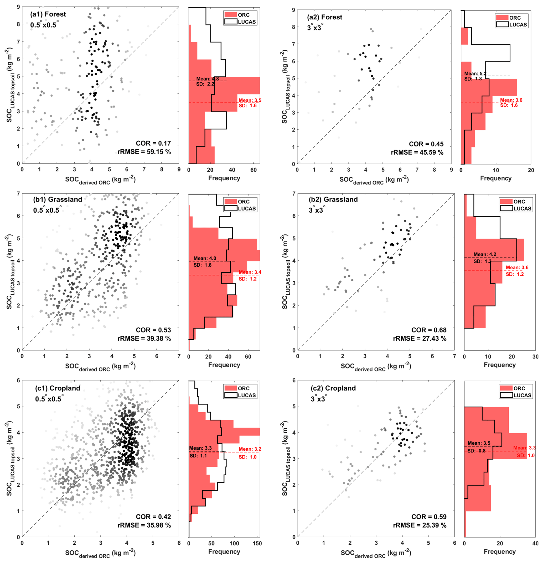
Figure 5 Scatterplots show the relationship between LUCAS topsoil data and derived ORCHIDEE soil organic carbon (SOC_{LUCAS topsoil} versus SOC_{derived ORC}, in kg m⁻²), along with their corresponding histograms. Plots are presented for two grid scales: 0.5° × 0.5° (a1, b1, c1) and 3° × 3° (a2, b2, c2). Darker colours indicate denser point concentrations. Complementary summary statistics are provided, including the mean and standard deviation (SD) values for each dataset, along with the correlation (COR) and relative root mean square error (rRMSE) between the two datasets. The corresponding maps are also presented in the Supplement (Figs. S2 to S4).

4 SOC change following land-use change (LUC)

Figure 6 compares observed and simulated SOC changes for different LUC transitions (see Table 2). During the C-to-G conversion, there is an increase in SOC stocks. However, the simulated results give a smaller increase than those observed in meta-analyses. Specifically, after a 100-year conversion period, the simulated SOC stocks increase on average by a mere 0.73 ± 0.09 kg m⁻², while the observed data show a much higher increase of 3.85 ± 1.33 kg m⁻². The G-to-C conversion leads to a decrease in SOC stocks. The model agrees with the observed change in direction but has a slower rate. Notably, the observed data display a wide range of confidence interval levels, and the simulated CRFs closely align with the upper boundary of the confidence interval. This highlights the difficulty of accurately capturing real-world SOC dynamics due to significant variability in the observed data.

Regarding G-to-F conversion, simulations using both TeBS and TeNE show different trends compared to the observed CRFs, as shown in the G-to-F_woFF and G-to-F_woFF subplots in Fig. 6. However, they consistently fall within the 95 % confidence interval, regardless of whether the forest floor is included in the analysis. In addition, the observed data for G-to-F conversions display considerable variability over time, which partly accounts for the difficulty in accurately modelling the true impact of this conversion type.

The conversions of C to F and F to C show opposite trends, as presented in the C-to-F_woFF, C-to-F_wFF, and F-to-C_woFF subplots in Fig. 6: C-to-F conversion leads to an increase in SOC and vice versa. Again, the averaged simulated CRF results align with the observed direction but indicate changes considerably slower than those reported in meta-analyses. In these two conversions, simulations with the TeBS forest appear closer to the observations than those with the TeNE forest.

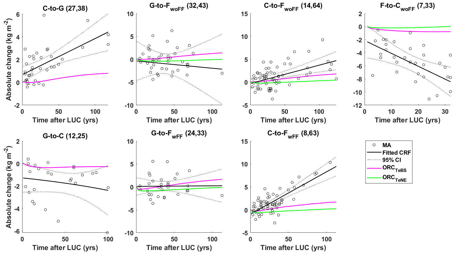
Figure 6 The absolute soil organic carbon changes (in kg m⁻²) from site observations in meta-analyses (black circles) and the fitted carbon response function (CRF; black lines) ±95 % confidence interval (dotted black lines) compared to simulated CRFs (magenta and green lines) for different land-use changes (LUCs; as presented in Table 2): cropland to grassland (C to G), grassland to cropland (G to C), grassland to forest (without and with forest floor G to F_woFF, G to F_wFF), cropland to forest (C to F_woFF and C to F_wFF), and forest to cropland (F to C_woFF). The first number in the parentheses indicates the number of study sites, and the second is the number of samples in the meta-analyses. Two distinct forest types, namely temperate broadleaf summergreen and temperate needleleaf evergreen, are considered for the forest sites in ORCHIDEE simulations (ORC_TeBS, ORC_TeNE).

Figure 6 suggests that the key model biases are the systematic underestimation of SOC gain during C-to-G transition and losses during G-to-C and F-to-C_woFF conversions. Multiple factors could contribute to these observed underestimations. As depicted in Fig. 7, soil erosion rate plays a pivotal role in the discrepancies observed across all considered LUC conversions among the six chosen factors. Conversely, temperature appears relatively less influential overall, except notably in the C-to-G conversion. Rainfall considerably influences the differences between observed and simulated absolute SOC changes after the conversions from C to G, C to F_woFF, and F to C_woFF. Soil phosphorus, on the other hand, demonstrates significance in the conversions of G to F_woFF, F to C_woFF (particularly for the TeNE forest), and C to G. Furthermore, the six chosen factors demonstrate a relatively consistent behaviour across the two forest types, as shown by the magenta and green bars for TeBS and TeNE (see Fig. 7).

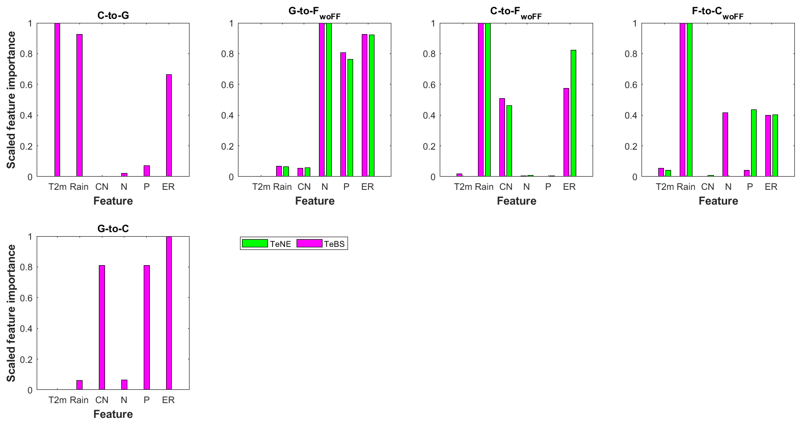
Figure 7 Scaled feature importance scores resulting from random forest (RF) analysis showing the relationship between model bias and potential influencing factors (i.e. temperature 2 m a.g.l. (T2m), rain, soil carbon-to-nitrogen ratio (CN), soil nitrogen (N), soil phosphorus (P), and soil erosion rate (ER)) for different land-use changes (LUCs): cropland to grassland (C to G), grassland to cropland (G to C), grassland to forest (without forest floor G to F_woFF), cropland to forest (C to F_woFF), and forest to cropland (F to C_woFF). Results for other conversions are not shown since RF shows poor performance (Table S7 in the Supplement). Each score is normalised within the range of 0 to 1, where 1 signifies the highest relevance, and 0 indicates the lowest importance. Two distinct forest types, namely temperate broadleaf summergreen and temperate needleleaf evergreen, are considered for the forest sites (TeBS, TeNE).

5 Discussion

5.1 Model performance for biosphere carbon stocks

The ORCHIDEE model shows a reasonable alignment with observed NPP, GPP (Fig. 1), and AGB trends (Fig. 2). Compared to observed data for all PFTs, the model shows narrower ranges. This dampened spatial variability may be due to the model's coarse resolution and constant parameter values for a given PFT, differing from species-specific observations affected by finer-scale environmental variations (Chang et al., 2013). The latter emphasises the need to incorporate a sufficiently large population of observed sites. Additionally, model–data disagreement can be linked to not-well-enough constrained values for PFT-specific parameters. For instance, our findings indicated that calibrating V_cmax and F_growthresp based on NPP and GPP observations for the TeNE forest type improved the model's performance in simulating AGB for this specific PFT (as shown in Fig. 2). Furthermore, our comparative analysis implied that employing temperate PFTs rather than boreal PFTs can enhance model performance in simulating the biomass of the boreal forests. This result suggests that certain PFTs, particularly those linked to boreal forest types, may be redundant in ORCHIDEE biomass simulations in the European context.

For SOC stock simulation, a Pearson's correlation of 0.4 between observed and simulated SOC values (Fig. 4) is significant, given the absence of certain controlling factors and processes in the model version used. This score is similar to that in other DGVM models (Wu et al., 2019; Seiler et al., 2022). For example, Wu et al. (2019) demonstrated a correlation coefficient of approximately 0.45 between LPJ-GUESS (a global dynamic ecosystem model) and SoilGrids (an observation-driven global soil dataset) on a global scale and lower correlation scores among different land cover classes. In this study, SOC scores varied among vegetation groups (Fig. 5), with lower correlations for forest sites. The inclusion of up to six PFTs in forest groups, with poorly determined classifications in observations, contributes to the model–data discrepancy. In contrast, grass and crop groups exhibit improved correlations with fewer PFTs and better distinction in LUCAS data (Ballot et al., 2023). Additionally, the smaller population of forest sites (Fig. 5) may account for the lower score compared with the other groups. Additionally, when examining different levels of resolution, we find that larger grid scales demonstrate a stronger correlation, which may be driven by climate patterns (Wang et al., 2023). At smaller scales, other environmental controls, like soil types, soil chemistry, topography, and management, become more important (Garten et al., 2007), which are not or only rudimentarily represented in ORCHIDEE. Implementing ORCHIDEE at a higher resolution using higher-resolution climate forcing (Anav et al., 2010; Lafont et al., 2012) can be challenging. This complexity arises from the fundamental reliance of the ORCHIDEE model on low-resolution environmental factors such as soil characteristics and erosion. Overcoming these inherent limitations in ORCHIDEE, as well as other DGVMs, can significantly improve model performance, particularly at more regional scales and higher spatial resolutions.

5.2 Impacts of LUC on soil carbon stocks

In pursuit of a more comprehensive evaluation, we explored the applicability of meta-analyses of site-level SOC changes for “pure” land cover transitions in assessing DGVMs' ability to simulate SOC stock responses to LUC. As discussed earlier, DGVMs, including ORCHIDEE, face challenges in simulating SOC stocks at a small scale, making it difficult to capture the SOC stock response at individual sites. Nevertheless, the model should be capable of matching average responses across broader regions.

In our comparison, we averaged the model responses over all grid cells encompassing the sites where LUC has occurred. This enabled us to compare the model's response to the meta-analysis data and its fitted CRF. Generally, the simulated results agree in terms of direction with observed data, notably the decrease in soil carbon stocks for G-to-C and F-to-C conversions and the opposite for C-to-G and C-to-F conversions (Fig. 6). As for G-to-F conversions, the simulations exhibit different trends from the observed CRFs but fall within the 95 % confidence interval (Fig. 6). In addition, the meta-analysis data exhibit considerable uncertainties, evident in the wide confidence intervals around the fits in Fig. 6. These uncertainties can be attributed to challenges related to data compatibility, methodological heterogeneity, and the diversity of ecosystems and LUC scenarios considered, as discussed in prior studies (Verburg et al., 2011; Deng et al., 2016; Fohrafellner et al., 2023). Therefore, while meta-analyses offer valuable insights, their interpretation requires careful consideration and integration with site-specific observations.

Despite this alignment in direction, there are noticeable discrepancies in the magnitudes of SOC stock changes between the simulated and observed CRFs, i.e. the underestimated SOC gain during C-to-G conversion and underestimated SOC losses during G-to-C and F-to-C_woFF conversions. These differences could potentially be attributed to various factors that the model may not fully capture. For instance, our findings indicate that soil erosion rate significantly influences the model bias among six selected potential factors. In addition, the influence of varying land management practices can substantially shape the model bias (Nyawira et al., 2016). These complexities underscore the challenges involved in accurately simulating local SOC dynamics. Further investigations or adjustments will be essential to reduce the biases and thereby enhance the accuracy of the model estimations. Additionally, our idealised assumption regarding the transition year in 1950 may introduce uncertainties to the model outputs. However, as shown in Sect. S1 of the Supplement, considering the actual transition year does not significantly enhance agreement with observations. This might be due to the limited number of available samples. It is also possible that the impact of climate change on LUC effects over the past century is not substantial. If the latter is true, using an idealised transition year should not create significant issues.

5.3 Challenges in model–data comparisons

Evaluating DGVM outputs against observational data is challenging, primarily due to constraints on the quantity and quality of existing long-term observational datasets. While observational data exist, their scarcity is evident, exemplified in Fig. 1, particularly in the instances of NPP and GPP sites for several PFTs like BoBS, TeBE, TeGC3, and BoGC3. Furthermore, as previously highlighted, substantial uncertainties persist in observed changes in SOC stocks when contrasted with anticipated changes. These limitations introduce intricacy into the process of calibrating and validating our models.

Another significant challenge arises from the long-lasting impact (e.g. >100 years) of historical LUC, particularly in the case of substantial events like erosion (Bakker et al., 2005; Borrelli et al., 2017). The absence of site history information hinders our ability to incorporate these effects into our simulations (Verburg et al., 2011). Disregarding the influence of major historical LUC events may lead to accurate simulations but for the wrong reasons. This approach further complicates our ability to predict changes in SOC stocks. In addition, failing to simulate LUC impacts accurately can have significant consequences for forecasting future land carbon balances and influencing decisions related to climate change mitigation and land management. To gain a more comprehensive perspective, we consider assessing the relative importance of SOC stock changes versus biomass carbon stock changes over, for instance, a 30-year horizon. This analysis can be relevant for initiatives like the European Green Deal (European Council, 2019), as it could offer essential guidance for shaping policies related to carbon sequestration, sustainable land-use practices, and preserving ecosystem health.

6 Conclusions

Our research investigated the ability of the DGVM ORCHIDEE model to reproduce what is known from experimental studies about LUC impacts on biospheric carbon. We performed various comparisons between simulations and experimental data, including on-site measurements and data from meta-analyses.

Discrepancies between the model and data can be attributed to several factors, such as the grouping of vegetation in DGVMs, which often use a limited number of PFTs, unlike the species-specific observations. The coarse model resolution also contributes to discrepancies. For example, our spatially explicit simulation of SOC stocks has a spatial resolution of 0.5°, whereas, in reality, SOC stocks and their controlling factors vary at a much smaller scale. Our analysis also identifies potential factors contributing to model bias when studying the impact of LUCs on SOC. Various factors, such as soil erosion rate, phosphorus, or rainfall, can influence each type of LUC. Further studies are needed to explore these impacts more comprehensively.

In summary, this study enhances our understanding of using DGVMs for studying carbon dynamics and provides insights for future model development and applications. While ORCHIDEE was our chosen model, this methodology can be readily applied to other DGVMs using the same protocol.

Appendix A: ORCHIDEE carbon module

Figure A1 presents the basic scheme of biospheric carbon cycling representation in ORCHIDEE. Simulated carbon dynamics include the exchange of carbon between the atmosphere and various carbon pools in vegetation biomass and soils. Carbon dynamics are simulated for each PFT individually, distinguishing eight vegetation biomass pools (leaves, roots, above- and below-ground sapwood, above- and below-ground heartwood, fruits, and a plant carbohydrate reserve), four litter pools (structural and metabolic litter above and below the surface), and three SOC pools (active, slow, and passive soil carbon). The turnover time of SOC and litter pools is determined by various factors, including temperature and humidity of the soil. The litter is produced through senescence and death, and the latter can also be related to LUC when the original vegetation is destroyed to make space for the new PFT. Further, carbon fluxes occur from litter to SOC pools and between the three SOC pools, with a part of the transferred carbon lost to the atmosphere through heterotrophic respiration. The model does not consider nutrient cycling, depth distribution of SOC, or soil carbon losses through leaching and erosion. Detailed formulations of the main processes represented in the version of ORCHIDEE used in this study can be found in Appendix A of Krinner et al. (2005).

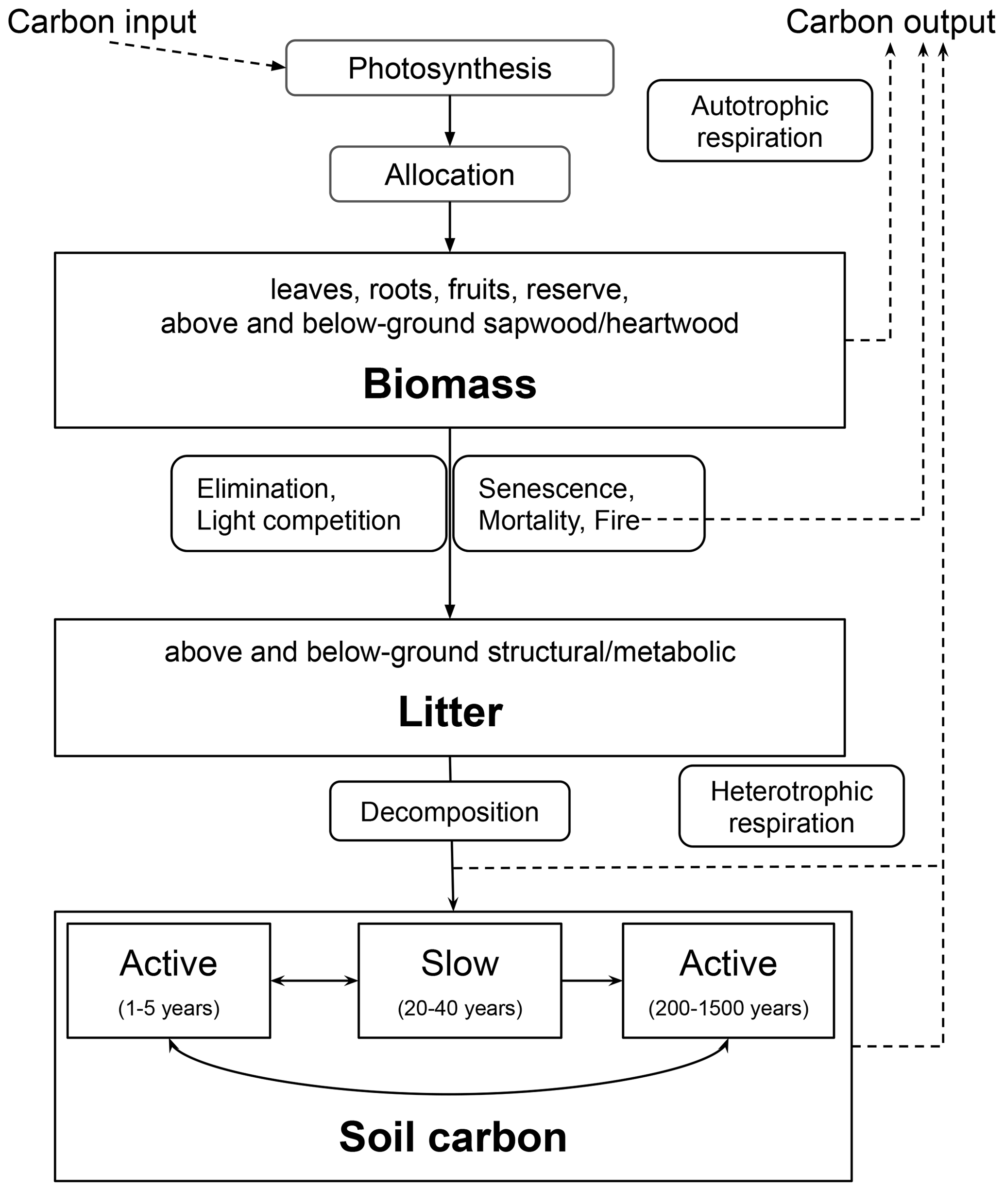
Figure A1 Basic structure of ORCHIDEE carbon module. The processes are denoted by rounded rectangles, while the reservoirs are represented by regular rectangles (accompanied by corresponding basic state variables in bold). The sub-processes are linked through carbon fluxes (depicted as black arrows). The figure is adapted from Krinner et al. (2005).