DeepPhenoMem V1.0: deep learning modelling of canopy greenness dynamics accounting for multi-variate meteorological memory effects on vegetation phenology

Vegetation phenology plays a key role in controlling the seasonality of ecosystem processes that modulate carbon, water and energy fluxes between the biosphere and atmosphere. Accurate modelling of vegetation phenology in the interplay of Earth's surface and the atmosphere is thus crucial to understand how the coupled system will respond to and shape climatic changes. Phenology is controlled by meteorological conditions at different timescales: on the one hand, changes in key meteorological variables (temperature, water, radiation) can have immediate effects on the vegetation development; on the other hand, phenological changes can be driven by past environmental conditions, known as memory effects. However, the processes governing meteorological memory effects on phenology are not completely understood, resulting in their limited performance of vegetation phenology represented in land surface models. A deep learning model, specifically a long short-term memory network (LSTM), has the potential to capture and model the meteorological memory effects on vegetation phenology. Here, we apply the LSTM to model the vegetation phenology using meteorological drivers and high-temporal-resolution canopy greenness observations through digital repeat photography by the PhenoCam network. We compare a multiple linear regression model, a no-memory-effect LSTM model and a full-memory-effect LSTM model to predict the whole seasonal greenness trajectory and the corresponding phenological transition dates across 50 sites and 317 site years during 2009–2018, covering deciduous broadleaf forests, evergreen needleleaf forests and grasslands. Results show that the deep learning model outperforms the multiple linear regression model, and the full-memory-effect LSTM model performs better than the no-memory-effect model for all three plant function types (median R² of 0.878, 0.957 and 0.955 for broadleaf forests, evergreen needleleaf forests and grasslands). We also find that the full-memory-effect LSTM model is capable of predicting the seasonal dynamic variations of canopy greenness and reproducing trends in shifting phenological transition dates. We also performed a sensitivity analysis of the full-memory-effect LSTM model to assess its plausibility, revealing its coherence with established knowledge of vegetation phenology sensitivity to meteorological conditions, particularly changes in temperature. Our study highlights that (1) multi-variate meteorological memory effects play a crucial role in vegetation phenology, and (2) deep learning opens up new avenues for improving the representation of vegetation phenological processes in land surface models via a hybrid modelling approach.

1 Introduction

Vegetation phenology characterizing key plant development stages such as leaf unfolding and leaf senescence plays a pivotal role as a primary regulator of ecosystem processes and land–atmosphere interactions (Peñuelas et al., 2009; Richardson et al., 2013; Piao et al., 2019). In response to global change, vegetation phenology has shown divergent shifts in diverse biomes (Menzel et al., 2006; Cleland et al., 2007; Wolkovich et al., 2012; Fu et al., 2015; Zhang et al., 2022), whilst at the same time exerting a substantial influence on ecosystem productivity and functions through the impact on biogeochemical processes, especially photosynthesis and carbon sequestration (e.g. Richardson et al., 2010) as well as ecosystem respiration (e.g. Migliavacca et al., 2015). Additionally, as green leaves are the primary interface for the exchange of energy, mass and momentum between the terrestrial surface and planetary layer (Richardson et al., 2012), vegetation phenology plays a fundamental role in controlling seasonal dynamics of water and heat fluxes between the land and the atmosphere (Peñuelas et al., 2009; Richardson et al., 2009; Puma et al., 2013; Jin et al., 2017; Buermann et al., 2018; Koebsch et al., 2020; Wu et al., 2022). Given the significance of vegetation phenology within the Earth system, an accurate representation of vegetation phenology in land surface models (LSMs) is crucial to enhance our understanding of ecosystem processes and their dynamics in response to climate change.

Over decades, many modelling efforts have been made to improve the development of accurate phenological models at the species-specific and plant-functional-type scale (White et al., 1997; Chuine, 2000; Jolly et al., 2005; Delpierre et al., 2009), including understanding the physiological mechanisms and environmental driving factors controlling phenology (Chen and Xu, 2012; Fu et al., 2020). Currently, vegetation phenological models mainly include statistical models and process-based models. These models are developed to simulate phenological events by integrating meteorological variables which are supposed to drive the processes of vegetation phenology, utilizing ground observations or phenological proxies derived from remote sensing vegetation index data. The most popular approach to represent phenology in land surface models is based on the accumulated growing degree days (GDD) (Lawrence et al., 2019; Asse et al., 2020; Pollard et al., 2020). The GDD model assumes that vegetation phenological events occur when the accumulated growing-degree-day sum fulfils a given requirement (i.e. a threshold of accumulated temperature over a certain time period). Considering the physiological processes, plants experience dormancy before entering the growing season, and thus chilling is considered to be essential to break dormancy in phenological models (Chuine, 2000; Menzel et al., 2011; Zhang et al., 2022). Besides temperature, the photoperiod and soil water availability have also been shown to be important drivers for vegetation phenology (Adole et al., 2019; Borchert et al., 2005; Chuine et al., 2010; Flynn and Wolkovich, 2018; Luo et al., 2020). Consequently, models based on GDD models have been improved by incorporating photoperiod and soil water availability effects, which have been applied in many LSMs, such as the Biome-BGC (BioGeochemical Cycles) model (Thornton et al., 2002; Thornton and Rosenbloom, 2005), JSBACH (Jena Scheme for Biosphere–Atmosphere Coupling in Hamburg; Mauritsen et al., 2019) and ORCHIDEE (ORganising Carbon and Hydrology In Dynamic Ecosystems; Krinner et al., 2005). Large uncertainties and biases in modelling phenology following these ad hoc concepts have been identified within LSMs and Earth system models (ESMs; Richardson et al., 2012; Jeong et al., 2012; Murray-Tortarolo et al., 2013; Lawrence et al., 2019; Peano et al., 2021), resulting in inaccurate estimations of primary productivity and the terrestrial ecosystem carbon and water cycle (Migliavacca et al., 2012).

To improve such phenology model performance, one has to consider more complex interactions of meteorological conditions that drive the vegetation phenological development. Phenology is triggered by meteorological conditions at various timescales. Instantaneous meteorological conditions like day-to-day variations in temperature, water, radiation can directly impact vegetation development. Additionally, longer-term and past meteorological conditions from the previous month or year have legacy effects on phenological changes. For example, a plant might face delays in budburst if the chilling requirements are not fulfilled (Ren et al., 2021). These lasting or delayed impacts are often referred to as memory effects, representing the impact of previous climate conditions on the present or future vegetation development. Studies have revealed that besides the well-known memory effect from temperature like GDD or chilling, other meteorological variables like precipitation or drought also have memory effects on vegetation growth and subsequent phenological appearance (Walter et al., 2011; Ogle et al., 2015; Ettinger et al., 2018; L. Liu et al., 2018; Lian et al., 2021). Due to the complexity and the interplay of various meteorological factors, current modelling efforts face a challenge in incorporating these multi-variate memory effects (which refer to the different memory effects that can be associated to different meteorological drivers) in a mechanistic manner.

Recently, data-driven methods including deep learning techniques have been used to investigate the influence of climatic factors on land surface processes (Forkel et al., 2017; Reichstein et al., 2019; Besnard et al., 2019; Kraft et al., 2019; Chen et al., 2021; Callaghan et al., 2021; Zhou et al., 2021), demonstrating their potential in capturing long-term temporal dependencies (Sutskever et al., 2014; Bahdanau et al., 2015). Deep learning models aim to consider the full spectrum of meteorological inputs making predictions and thus hold promise in capturing long-term temporal dependencies from multiple variables (Besnard et al., 2019; Kraft et al., 2019). A recent study has already indicated that the deep learning technique is capable of improving the predictability skill of vegetation phenology with respect to conventional methods (Zhou et al., 2021). The long short-term memory network (LSTM), a type of deep learning neural network, is designed specifically for sequence prediction problems that deal with the memory effect (Hochreiter and Schmidhuber, 1997). Also, time series of consistent and widely distributed phenological near-surface observations are now long enough so that they reflect short- and long-term sensitivities to meteorological conditions. Specifically, the continuous daily dataset from the PhenoCam initiative (Richardson et al., 2018), obtained from images of near-surface digital cameras, offers opportunities to apply deep learning methods for developing vegetation phenology models that account for the memory effects of multiple meteorological variables (Richardson et al., 2018; Seyednasrollah et al., 2019).

We propose to use the PhenoCam data and the LSTM framework to develop a deep learning model that is capable of not only predicting specific transition dates but also forecasting the state of the canopy greenness throughout the entire year. Most current phenology modelling studies focus on phenological transition dates only, such as the onset of budburst, flowering or leaf senescence (Chuine, 2000; Delpierre et al., 2009; Fu et al., 2020). These phenological models effectively capture the processes that lead to individual phenological events but fail to overlook the dynamical nature characterizing the continuous phenological development throughout the entire annual cycle, where the phenological state itself could influence the subsequent phenological development (Fu et al., 2014). Conversely, models targeting the whole seasonal trajectory (White et al., 1997) possess the capability to provide continuous predictions of the phenological development state that decisively influences other biogeochemical and biophysical processes at the land surface.

More specifically, in this study, we focus on the modelling of the whole seasonal trajectory of canopy greenness but also the prediction of transition dates in the annual cycle of canopy greenness. Overall, our key objective is to develop a robust deep learning vegetation phenology model on the basis of a LSTM to characterize the memory effects of multiple meteorological variables on canopy greenness using the PhenoCam observations. We also build a statistical model as the baseline to evaluate the performance of our machine learning model. Our study focuses on addressing the following research questions: (1) can deep learning models perform better than statistical models? And can deep learning models accounting for memory effects of multiple meteorological variables outperform models that do not account for such memory effects? (2) Do deep learning models successfully capture temporal variations on different timescales of canopy greenness and vegetation phenology? (3) Can deep learning models provide meaningful interpretations of the underlying physical and biological relationships between vegetation greenness, phenology and a changing climate?

2 Materials and methods

2.1 PhenoCam data

The phenological data used in this study are acquired from the PhenoCam dataset v2.0 (https://daac.ornl.gov/VEGETATION/guides/PhenoCam_V2.html, last access: 29 August 2024, Seyednasrollah et al., 2019). The dataset is derived from digital images photographed by automated and high-frequency digital cameras at half-hour intervals. These images are analysed to calculate the green chromatic coordinate (GCC), which is the ratio of the green channel digital numbers to the total digital values of the digital RGB images within a predefined region of interest. GCC serves as an indicator of canopy greenness, with variations primarily due to changes in photoprotective pigments, which cause the variation in canopy greenness. For example, the changes in photoprotective pigments cause the canopy to appear more “red” in winter (indicating low GCC) compared to summer.

To construct a daily GCC time series, we use the 90th percentile of daily GCC values, reducing the impact of atmospheric conditions on illumination. This daily GCC time series is used in this study to represent the canopy greenness development and senescence. Specifically, we select the GCC time series from Type I observation sites that follow a standard protocol to ensure data quality and continuity (Richardson et al., 2018). To ensure robust data, we exclude yearly GCC data for years with more than 20 d of missing digital images. We further select sites with continuous observations available for more than 5 years. Missing data in the GCC time series are interpolated using a cubic spline interpolation method (Hall and Meyer, 1976). Additionally, we apply a locally weighted scatter plot smoothing method to reduce noise in the GCC time series (Cleveland, 1979). Our study focuses on three main plant functional types (PFTs): deciduous broadleaf forest (DB), evergreen needleleaf forest (EN) and grassland (GR), with observed GCC ranges of 0.30–0.46 for DB, 0.32–0.43 for EN and 0.30–0.43 for GR. Ultimately, a total of 50 sites and 317 site-year observations during 2009–2018 are used in the analysis. Of these, 28 sites with 178 site-year observations are DB sites, 13 sites with 82 site-year observations are EN sites and 9 sites with 57 site-year observations are GR sites. The spatial distribution of the study sites and test sites for each PFT is shown in Fig. 1.

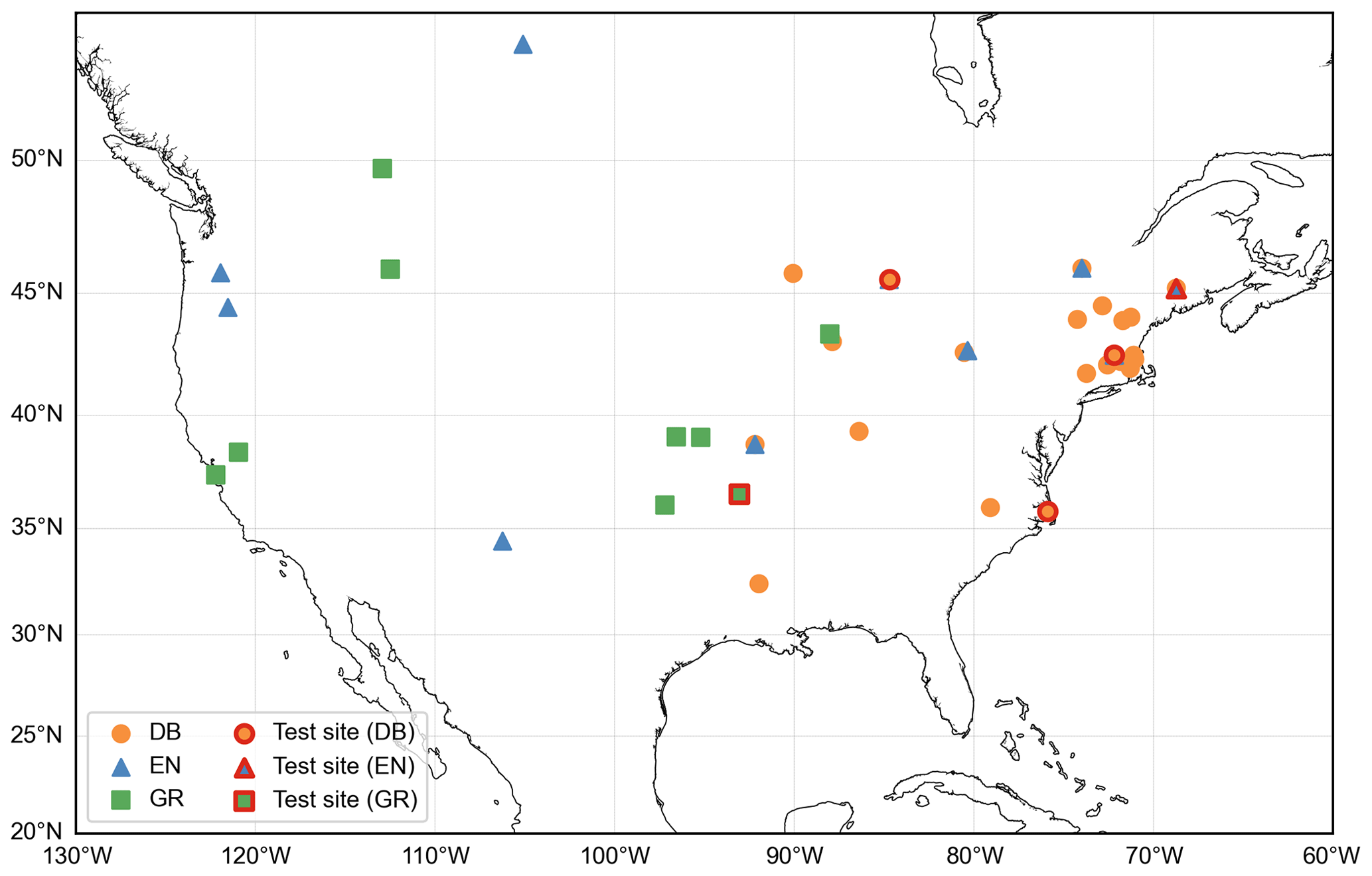
Figure 1 Geographical distribution of study sites for deciduous broadleaf forest (orange circles), evergreen needleleaf (blue triangles) and grassland (green squares). The test sites are specifically highlighted within a red border.

2.2 Explanatory variables

The daily meteorological variables were obtained from the station-level Daymet dataset (https://daymet.ornl.gov/, last access: 29 August 2024). These variables include daily minimum temperature (T_min), daily maximum temperature (T_max), daily day length (DL), daily precipitation (P), daily water vapour pressure of the air (e_a) and daily shortwave radiation (R). We extract time series of these meteorological variables for each studied PhenoCam site. Given that the soil moisture might have memory effects on vegetation canopy greenness development, it should be included as a driver in the model. In our study, six dynamic variables are used, including T_min, T_max, DL, R, vapour pressure deficit (VPD) and soil moisture index (SMI). The daily VPD is the difference between the saturation pressure of water (e_s, calculated from the daily mean temperature) and the actual water vapour pressure of the air (e_a), calculated following Eqs. (1) and (2) (Alduchov and Eskridge, 1997). Due to the lack of measured soil moisture data, we have utilized a 30 d backward running mean of precipitation, applying decreasing weights (from 0 to 1) to days in the past 1 month, as a proxy for soil moisture. This index has been demonstrated to serve effectively as a proxy for soil moisture where direct soil moisture measurements are unavailable (Migliavacca et al., 2011). The daily SMI is computed using a proxy of the sum of precipitation over the previous month (Eq. 3). Additionally, two static variables, mean annual temperature (T_mean) and mean annual precipitation (P_mean), are derived from the records of these two variables in PhenoCam dataset.

$$\begin{array}{}\text{(1)}& {\displaystyle }\mathrm{VPD}=e_{\mathrm{s}}-e_{\mathrm{a}}\text{(2)}& {\displaystyle }{e}_{\mathrm{s}}=\mathrm{0.61094}\times e^{\frac{\mathrm{17.625}T}{T+\mathrm{243.04}}},\end{array}$$

where e_s and e_a are saturated and actual vapour pressure, respectively (kPa). T is the mean daily air temperature (°C).

$$\begin{array}{}\text{(3)}& {\mathrm{SMI}}_t={\displaystyle \frac{{\sum }_{i=\mathrm{0}}^{\mathrm{30}}(P_{t-i}\times \frac{\mathrm{30}-i}{\mathrm{30}})}{\mathrm{31}}},\end{array}$$

where SMI_t is the soil moisture index on day t, P_t−i is the precipitation on day (t−i) and i is the number of days away from the day of t.

2.3 LSTM modelling approach

Our goal is to predict the whole seasonal trajectory of the canopy's green chromatic coordinate (GCC) from the time series of the eight predictor variables using one model per PFT for multiple sites. To make this task feasible, we subtract the winter baseline value (the mean of the minimum GCC values in available years) of GCC at each site and PFT, making the measurements more comparable across sites. Further, the predictor variables and targets (GCC) are globally normalized using a min–max transformation for each PFT.

To ensure that our models learn relationships that can be generalized, we evaluate them on unseen data in space and time. For the spatial generalization, we hold out 10 % of all studied sites as unseen test sites. Furthermore, we use all data from the year of 2018 for each PFT as our temporal test dataset. The division of the data is illustrated in Fig. S1. Additionally, we divide the dataset into samples consisting of 2 years of input predictor variables (accounting for potential memory effects of meteorological variables from previous 1 year to the current year), along with 1 year of GCC observations corresponding to the second year of input.

To capture the relationship between the meteorological variables and the GCC, we employ a LSTM network (Hochreiter and Schmidhuber, 1997). We choose this method for several reasons. Firstly, we expect a highly non-linear relationship between the meteorological variables and observed canopy greenness, necessitating a flexible, nonparametric model such as a neural network (Hornik et al., 1989). Secondly, the representation of dynamic meteorological memory effects on canopy greenness requires a model that can represent temporal interactions across scales. For this purpose, we utilize a recurrent neural network (RNN), specifically the LSTM, which has demonstrated strong performance in prediction-related problems involving time-series data (Wu et al., 2017; Besnard et al., 2019; Kraft et al., 2019, 2022).

In our study, we employ a single-layer LSTM with 128 nodes, followed by one fully connected (output) layer and preceded by one fully connected (input) layer. The mean squared error between the predicted and the observed GCC is optimized using the gradient-based AdamW (Loshchilov and Hutter, 2019), an algorithm that adds decoupled weight decay to the Adam (Kingma and Ba, 2015) optimizer. We train an ensemble of models to reach a more stable prediction. During the model development phase, we utilized a leave-one-site-out cross-validation strategy, applied 25-fold for the DB, 12-fold for the EN and 8-fold for the GR datasets. This approach was integral to identifying the most effective model architectures and hyperparameters, ensuring robustness across various sites. Additionally, we employed these validation datasets for early stopping to prevent overfitting. Specifically, we stop the training when the performance no longer improves on the left-out validation set of 150 epochs (an epoch refers to one complete pass through the entire training dataset). Furthermore, we decay the learning rate (a hyperparameter that determines the size of the steps taken during the optimization of a model) of, initially, 0.01 by a factor of 0.9 after each epoch. For testing we use the mean of the ensemble of LSTMs as the prediction for the GCC.

To quantify the importance of the memory effects in the model, we additionally train our model on the same dataset, with all data being randomly shuffled in the time dimension (Besnard et al., 2019; Kraft et al., 2019). In this dataset the “instantaneous” relation between the inputs and outputs of the current day is unimpaired, but the effects of previous days cannot be learned, as these days are random. This LSTM model does not consider the memory effects, referred to as the no-memory-effect LSTM model, M₀. In contrast, the original model, which has access to the full history of the input variables, is referred to as the full-memory-effect LSTM model, M_full. The framework of our LSTM model in predicting canopy greenness GCC using six dynamic and two static predictors is illustrated in Fig. 2.

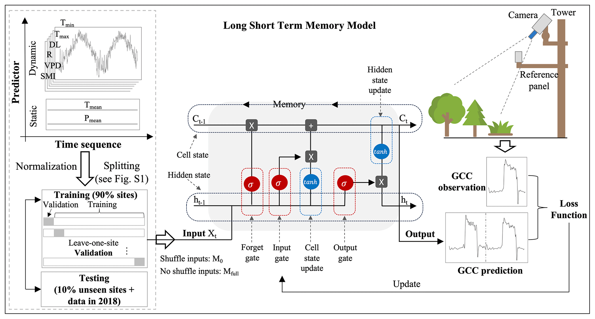
Figure 2 The framework of canopy greenness modelling using LSTM. The LSTM is composed of a forget gate, an input gate, an output gate, and a candidate and hidden state. The LSTM networks are adapted from Christopher Olah, http://colah.github.io/posts/2015-08-Understanding-LSTMs/ (last access: 29 August 2024).

2.4 Model evaluation

To assess the modelling ability of deep learning models, we develop a baseline model using multiple linear regression (MLR) between the eight predictor variables and GCC (Eq. 4). The MLR model is trained and tested in the same training and testing dataset as the LSTM models.

$$\begin{array}{}\text{(4)}& \begin{array}{rl}\mathrm{GCC}& =a\times T_{\min }+b\times T_{\max }+c\times \mathrm{DL}+d\times R+e\\ & \times \mathrm{VPD}+f\times \mathrm{SW}+g\times T_{\mathrm{mean}}+k\times P_{\mathrm{mean}}+\mathrm{res},\end{array}\end{array}$$

where GCC is our target; T_min, T_max, DL, R, VPD, SW, T_mean and P_mean are predictor variables; and res is the residual.

For model evaluation, we primarily use the root mean square error (RMSE) and the coefficient of determination (R²) for model evaluation. These metrics are calculated based on the predicted and observed GCC at each site for each PFT. We compare the model performance of all models in the testing dataset and select the best model for each PFT by R². For the best models, we evaluate their performance in simulating (1) GCC observations, (2) GCC temporal variation and (3) phenological transition dates in testing datasets. GCC temporal variation includes variation on three timescales: daily variation, monthly mean GCC variation and interannual variation of the anomalies of median GCC. For daily variation, we also calculate the daily anomalies for observations and LSTM models. For the monthly GCC variation, we further compare the mean monthly canopy development rate (V_GCC) during studied years between observed and predicted GCC time series. The rate of canopy development for each month (from February to December) is calculated at the monthly scale from the GCC time series using Eq. (5).

$$\begin{array}{}\text{(5)}& V_{\mathrm{GCC}\left(t\right)}={\mathrm{GCC}}_t-{\mathrm{GCC}}_{t-\mathrm{1}},\end{array}$$

where t is time (month), and GCC_t and GCC_t−1 are the mean GCC values for a given year at month t and t−1, respectively.

The phenological transition dates are estimated intending to define the start of season (SOS) and the end of season (EOS) for 1 year. We choose the dates corresponding to 30 % of the seasonal amplitude (from the 5th percentile to the 95th percentile) through greening rising and falling to represent the SOS and EOS. SOS and EOS transition dates are estimated from both the predicted and observed GCC time series.

2.5 Model sensitivity analysis

In order to gain insights into the physical implications of deep learning models, we conduct two simple experiments to assess the model sensitivity to meteorological drivers. First, we increase (warming) and decrease (cooling) temperature (T_min and T_max) by 4 °C throughout the year while keeping all other predictors unchanged. Another experiment involves the same temperature adjustments for T_min and T_max but with the VPD varying based on mean temperature while keeping other predictors constant. We then compare the annual canopy greenness cycles under warming and cooling conditions with the actual observations. Furthermore, to better understand how vegetation phenology shifts in response to a warming environment according to the LSTM models, we estimate the SOS and EOS in these two experiments. We evaluate the differences between the treatment of 1 °C warming and the observations for SOS and EOS.

3 Results

3.1 Model performance

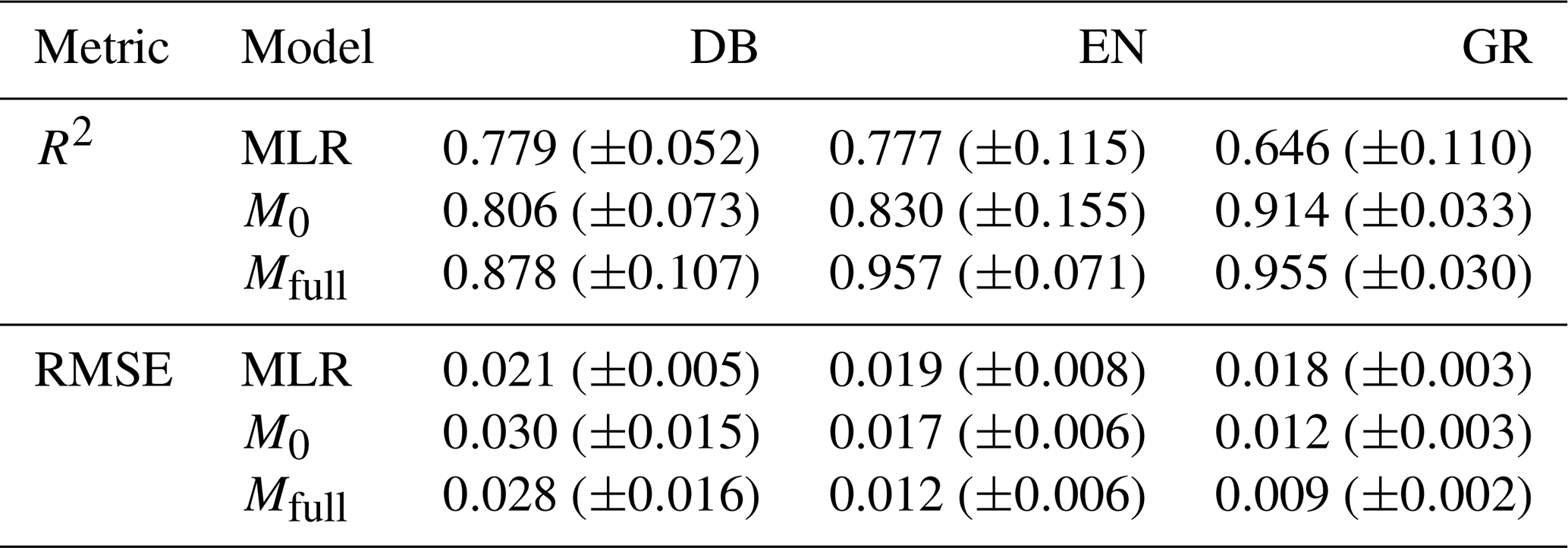
A comparison of the model performance is conducted between the statistical MLR model and the LSTM models (including the no-memory-effect LSTM model M₀ and the full-memory-effect LSTM model M_full) on the test dataset for deciduous broadleaf (DB), evergreen needleleaf (EN) and grassland (GR) (Table 1). The LSTM models achieve a better performance for predicting the GCCs than the MLR model for all PFTs (Table 1). The coefficient of determination R² between modelled and observed canopy greenness GCC is much higher in LSTM models than MLR, with the median R² increased from MLR to LSTM from 0.779 to more than 0.806 for DB, from 0.777 to more than 0.830 for EN and from 0.646 to more than 0.914 for GR. Similarly, the root mean square error (RMSE) values corroborated the R² findings, demonstrating that LSTM models generally exhibit lower prediction errors than the MLR model. In conclusion, LSTM models significantly enhance the accuracy of GCC predictions across all three PFTs when compared to the baseline MLR model.

Table 1 Coefficient of determination (R²) and root mean square error (RMSE) comparisons (ensemble median ±SD estimate of all study sites) for the multiple linear regression model (MLR), no-memory-effect LSTM model (M₀) and full-memory-effect LSTM model (M_full) on the test dataset for deciduous broadleaf (DB), evergreen needleleaf (EN) and grassland (GR).

Furthermore, comparing the two different LSTM models, the full-memory-effect model M_full exhibits superior performance in simulating GCC compared to the no-memory-effect model M₀ across all three PFTs (Fig. 3). The median R² of all studied sites in the full-memory-effect model exceeds 0.85, specifically 0.878 for DB, 0.957 for EN and 0.955 for GR. This represents an improvement in model performance of 8.9 % for DB, 15.3 % for EN and 4.5 % for GR, compared to the no-memory-effect model, with R² of around 0.806 (DB), 0.830 (EN) and 0.914 (GR). Similarly, there is a reduction in bias of 12.5 % (RMSE decreased from 0.036 in M₀ to 0.032 in M_full) for DB, 15.4 % (RMSE decreased from 0.015 in M₀ to 0.013 in M_full) for EN and 37.5 % (RMSE decreased from 0.011 in M₀ to 0.008 in M_full) for GR in full-memory-effect models. These findings suggest that considering memory effects from multiple meteorological factors can enhance the model performance in simulating GCC compared to models without considering memory effects.

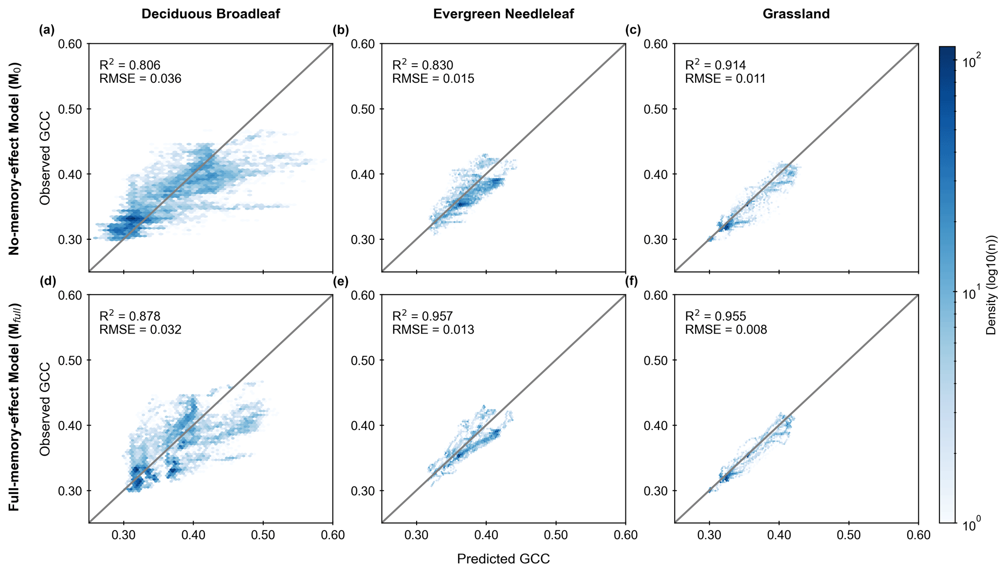
Figure 3 Model performance of GCC time-series estimation using the no-memory-effect model (M₀; a, b and c) and the full-memory-effect model (M_full; d, e and f) in all test datasets for deciduous broadleaf (DB), evergreen needleleaf (EN) and grassland (GR). The colour indicates the density of points (light blue is lower density, and dark blue is higher density). The solid grey lines denote the 1:1 line.

The performance of LSTM models on unseen test sets, both spatially and temporally, shows that the full-memory-effect LSTM model M_full outperforms the no-memory-effect LSTM model M₀ in predicting GCC for unseen site(s) and unseen years across all three studied PFTs (Fig. 4). Specifically, when evaluating performance on unseen sites, M_full consistently exhibits higher median R² values compared to M₀, with improvements of 9.3 %, 13.5 % and 3.5 % for DB, EN and GR, respectively. Similarly, for predictions across unseen years, M_full demonstrates substantial enhancement in predictive accuracy, with median R² values increasing from 0.805 to 0.874 (an 8.6 % improvement) for DB, from 0.824 to 0.956 (a 16 % improvement) for EN and from 0.914 to 0.964 (a 5.5 % improvement) for GR. The t test comparing M₀ and M_full across all test sets and PFTs indicates a significant difference (P<0.05), confirming M_full's superior performance. These findings underscore the robustness of the model in accurately forecasting GCC time series, even when faced with previously unobserved spatial and temporal contexts.

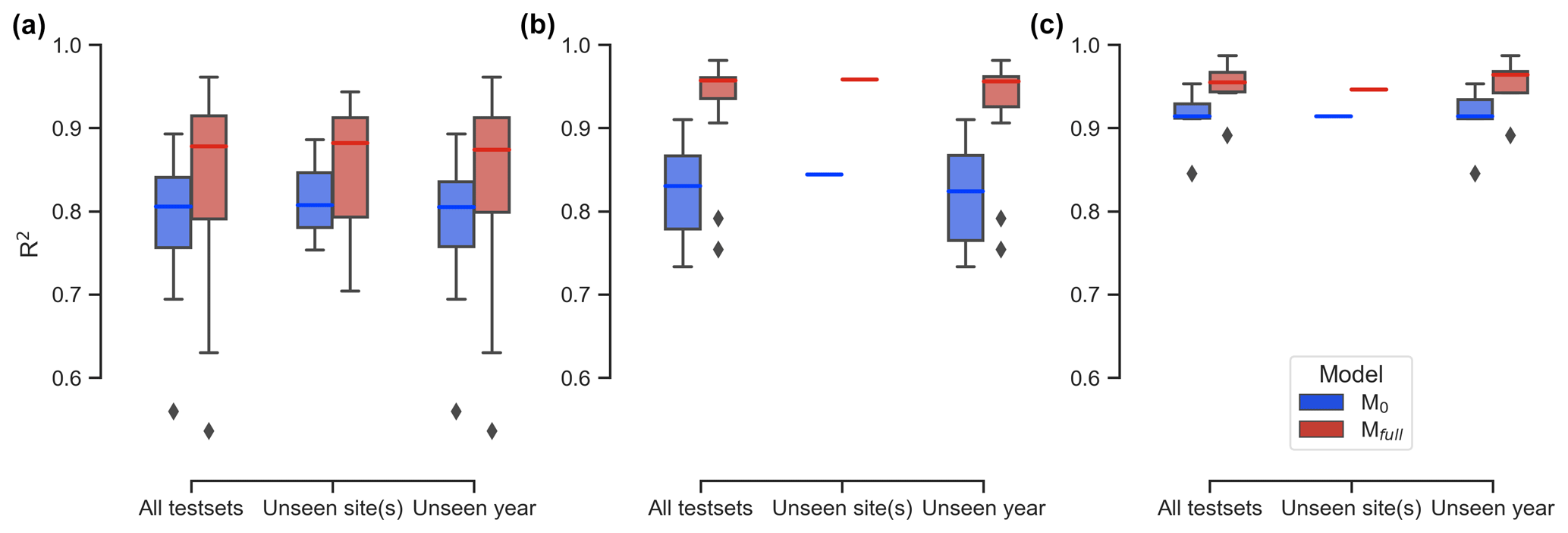
Figure 4 Coefficient of determination (R²) comparisons between the no-memory-effect model (M₀: blue box) and the full-memory-effect model (M_full: red box) in all test sets, for unseen sites and unseen years for deciduous broadleaf (DB; a), evergreen needleleaf (EN; b) and grassland (GR; c). The rhombus in the figure represents the outliers, which are defined as the points beyond 1.5 times the interquartile range (the difference between the 75th and 25th percentiles).

3.2 Modelling temporal variability of GCC at unseen sites: daily to interannual timescales

LSTM models can capture the GCC canopy greenness temporal dynamics, with an initial increase followed by a decrease during the growing season. This is illustrated in Fig. 4, which displays the observed and predicted daily variability of GCC, the daily GCC anomaly, the seasonal variability of GCC and its development rate, and the interannual variability of GCC anomalies at unseen sites from 2009 to 2018 using LSTM models. The predicted daily variability of GCC shows a strong correlation with observations across multiple years, with a significant correlation coefficient (r) above 0.9 (Fig. 5a–c) in M_full. Conversely, M₀ shows increased noise in daily GCC variability, displaying larger biases in predicting both GCC peaks and minimum values, particularly evident for DB (Fig. 5a). From the predictions of daily GCC anomalies which remove the mean seasonal cycle (Fig. 5d–f), we further find that M_full performs better than M₀ in capturing the daily fluctuation, though it is still not as good at predicting the daily GCC anomalies as we expected. The R² between observed and predicted GCC anomalies is higher in M_full than in M₀ for DB (M₀: 0.0007, M_full: 0.02), EN (M₀: 0.03, M_full: 0.22) and GR (M₀: 0.07, M_full: 0.32). However, a discrepancy between observed and predicted absolute GCC at the daily scale is observed for EN in the unseen site, where the predicted GCC is overestimated compared to the observation in both M_full and M₀ (Fig. 5b).

The overall seasonal cycle of monthly GCC shows a good match between the observation and prediction by LSTM models. The observed GCC typically starts to increase in March (GR) or April (DB and EN), peaks in June (DB and GR) or July (EN), and gradually decreases until November (DB and GR) or December (EN) (Fig. 5g–i). Both M_full and M₀ can effectively capture this seasonal pattern for EN and GR. However, for DB, the M_full model predicts a similar seasonal dynamic pattern of GCC to observations, depicting greening up before June or July followed by greening down until November or December, while M₀ predicts a peak in greenness occurring in July which diverges from observation (Fig. 5g). Similarly, the development rate of monthly GCC shows similar performance to the seasonal cycle of monthly GCC. The largest increase in observed GCC occurs in May during the greening-up period for all three vegetation types, while the speed of greenness decreases significantly accelerates around October (grey box in Fig. 5g–i). The LSTMs predict that developed rates in greening up and down exhibit a similar pattern to the observations for EN and GR (red box in Fig. 5g–i). However, for DB, both M_full and M₀ predict the highest development rate in June during the green-up period and in September during the green-down period, in contrast to observations which indicate peak rates in May and October, respectively.

The predicted interannual variability of maximum GCC anomalies shows that LSTM models with both full memory effects and no memory effects can generally forecast trends of interannual variability of maximum GCC for EN and GR (Fig. 5k–l). However, an increasing trend (0.026 per decade) in greenness is observed in maximum GCC anomalies from harvardbarn2 for DB during the period from 2012 to 2018 (see Fig. 5j), and this trend is well predicted by the M_full model (0.015 per decade) but failed in the M₀ model (−0.004 per decade). Specifically, from 2012 to 2015, the observed maximum GCC exhibits a continual increase, whereas M₀ indicates a continual declining maximum GCC (see Fig. 5j). Furthermore, a larger bias is found in M₀ compared to M_full in predicting the annual maximum GCC for DB.

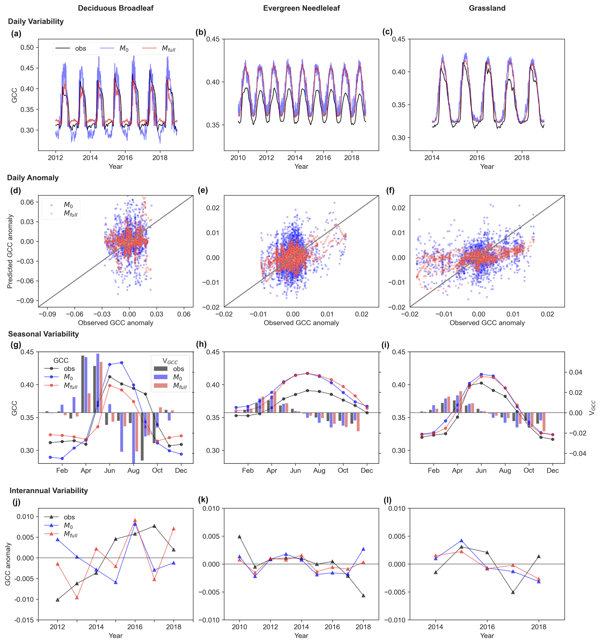
Figure 5 Observed (obs; grey) and predicted (M₀: blue, M_full: red) daily (a, b, c), seasonal (g, h, i) and interannual (j, k, l) variability of canopy greenness (GCC) and daily GCC anomaly (d, e, f) for deciduous broadleaf (DB), evergreen needleleaf (EN) and grassland (GR) in unseen sites (DB: harvardbarn2, EN: howland1, GR: bullshoals). In panel (d)–(f), the solid grey lines denote the 1:1 line. In panel (g)–(i), the development rate of monthly GCC (V_GCC) is represented by bar plots (right y axis; red bar: observed V_GCC; red bar: predicted V_GCC). In panel (j)–(l), the interannual variability of annual maximum GCC anomalies is shown.

3.3 Modelling the vegetation canopy phenological transition dates in unseen sites

Figure 6 illustrates that M_full can capture the interannual variability of phenological transition dates, outperforming M₀. Regarding the start of season (SOS) (Fig. 6a, b, c), M_full consistently exhibits the same shift direction (sign of the anomaly) as observations in the majority of years. Specifically, we observe concordance in the direction of advance or delay between prediction and observation in 5 out of 7 years (71 % of the years) for DB. Similarly, the predicted SOS shifts agreed well with the observations in more than 80 % years for EN (89 % of the years) and GR (80 % of the years). Moreover, a high correlation is evident between the M_full-predicted interannual variability of SOS anomaly and the observed interannual variability of SOS anomaly. The correlation coefficient between observed and predicted interannual variability of SOS anomaly reaches up to more than 0.9 for EN and GR. Further, the observed delay of SOS with the trend of 2.1 d yr⁻¹ is also reproduced well by the M_full (predicted trend is 1.2 d yr⁻¹) in howland1 for EN during 2010 to 2018 (Fig. 6b). Conversely, compared to M_full, M₀ exhibits poor performance in capturing the shift direction and lower correlation between the predicted interannual variability of SOS anomaly and the observed interannual variability of SOS anomaly.

As for EOS, good agreements between the predicted interannual dynamics of EOS anomalies by M_full and the observed ones are found in DB and EN, although not in GR (Fig. 6d–f). Firstly, M_full-predicted shift directions of EOS in most years (over 80 %) are consistent with the observed shifts for each PFT. For DB, 86 % of years are showing the same shift direction of advance or delay between observed and predicted EOS. For EN and GR, the percentages are 89 % and 80 %, respectively. On the other hand, we find a positive correlation between observed and M_full-predicted EOS anomalies for DB and EN. The observed delayed trend (2.7 d yr⁻¹) for DB in harvardbarn2 is also well predicted (1.6 d yr⁻¹) by the M_full. Interestingly, M_full also captures the larger advancement of EOS observed in 2018 compared to the mean EOS for EN, indicating its capability to capture extreme interannual anomalies. Compared to M_full, M₀ shows a relatively poor performance, displaying larger bias in its predictions.

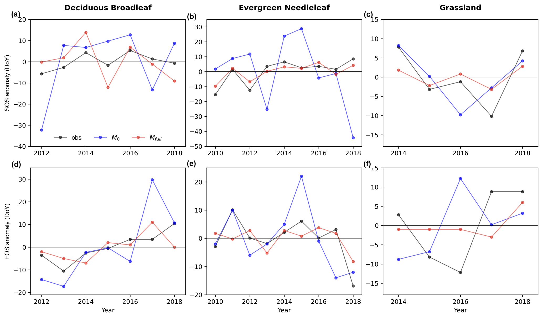
Figure 6 Observed (obs; black line) and predicted (M₀: blue, M_full: red) the interannual variability in anomaly of start of season (SOS; a, b, c) and end of season (EOS; d, e, f) for deciduous broadleaf, evergreen needleleaf and grassland in unseen sites (DB: harvardbarn2, EN: howland1, GR: bullshoals).

3.4 The model sensitivity analysis

The model sensitivity analysis indicates that the full-memory-effect model M_full can simulate the GCC response to temperature well. Figure 7 illustrates the temperature sensitivity of GCC in the LSTM model M_full for all three PFTs studied here. Comparison of experiments with warming (red line, Fig. 7a, b, c) and cooling (blue line, Fig. 7a, b, c) alone (increasing or decreasing 4 °C) to the unchanged temperature (±0 °C) control (grey line, Fig. 7a, b, c) reveals that warming led to a greener and longer greenness season, while cooling caused a less green and shorter vegetation season for the three PFTs studied (Fig. 7a, b, c). When VPD varies with temperature, high temperature along with the high VPD does not have a significant effect on the greenness and length of vegetation period. During the greenness rising and falling period, the canopy greenness is very similar to the actual GCC cycle (the control) for the three PFTs, but the peak greenness is lower than the actual GCC peak values, especially for DB and GR (Fig. 7d, e, f). In the cooling and lower VPD treatment, it shows similar trends with the cooling condition but unchanged VPD. Cooling and a lower VPD result in declining canopy greenness and shortened vegetation periods during the growing season.

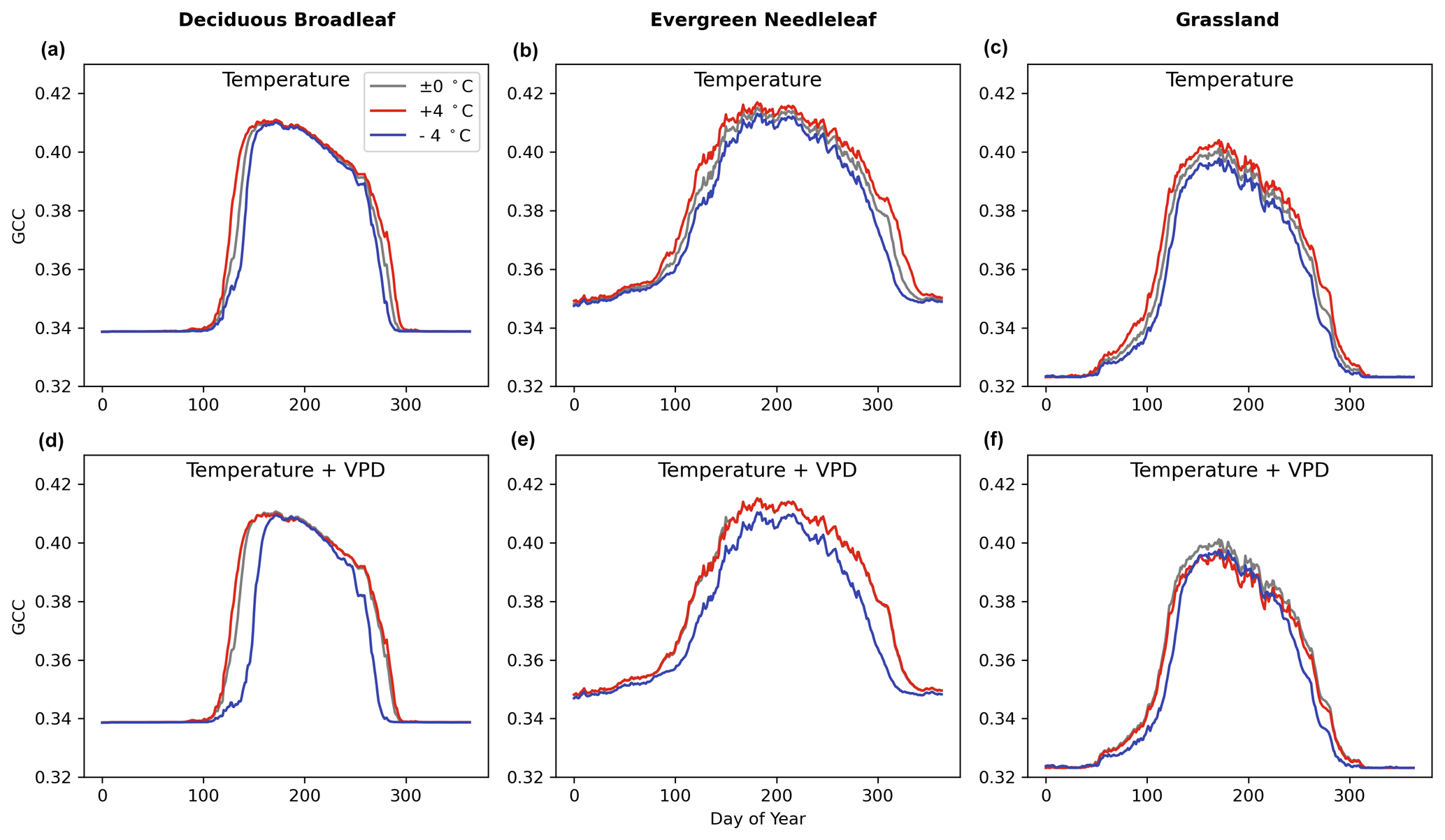
Figure 7 The sensitivity of canopy greenness (GCC) to temperature change only and both temperature and VPD change under 4 °C warming/cooling (red line/blue line) throughout the year using M_full for deciduous broadleaf (in howland2), evergreen needleleaf (in laurentides) and grassland (in bullshoals).

Furthermore, we also examine the temperature sensitivity of phenological events (SOS and EOS) (Fig. 8). A 1 °C increase in temperature throughout the year resulted in an earlier start of the season (Fig. 8a) and delayed end of the season (Fig. 8b), regardless of low or high VPD. Under warm conditions alone, SOS appears to be 1 d earlier on average, while under warm and high VPD conditions, it shifts to 2 d earlier. The 1 °C temperature increase has a similar effect on EOS compared to the 1 °C increase accompanied by varied VPD. Through Student t tests on the means of the two distributions, no statistically significant (p=0.12 (SOS), p=0.69 (EOS)) differences in the means are found, indicating that temperature is the most influential meteorological factor affecting the start and end of the season.

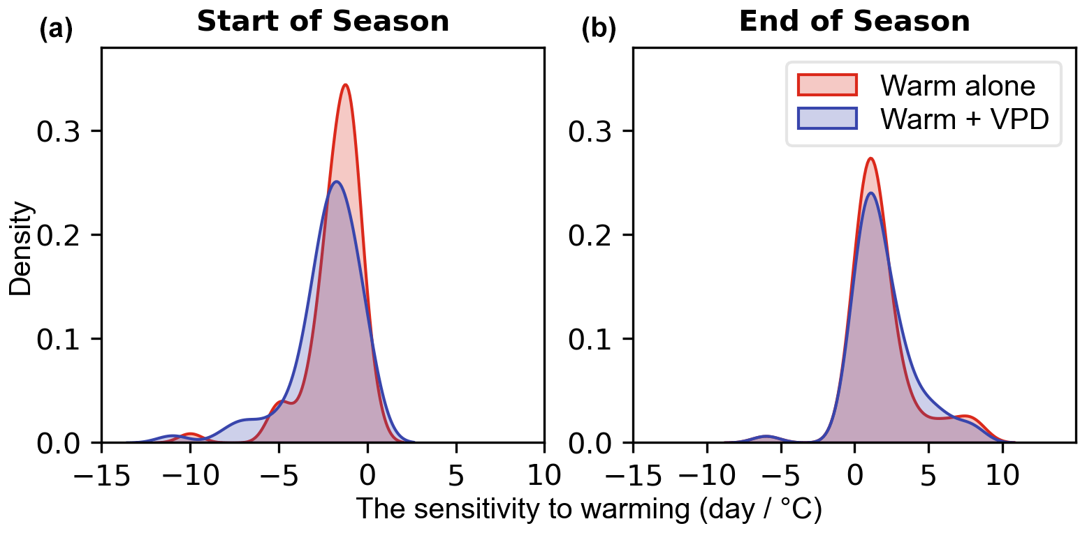
Figure 8 Temperature sensitivity of start of season (SOS; Fig. 8a) and end of season (EOS; Fig. 8b) under warm conditions alone (red) and warm and high VPD conditions (blue) over all three PFTs.

4 Discussion

4.1 Meteorological memory effects on vegetation canopy greenness

In our study, we have presented a new way to simulate canopy greenness dynamics by applying a data-driven LSTM model accounting for multi-variate meteorological memory. We find that multi-variate meteorological memory is of importance in developing vegetation phenological models. The impact of meteorological factors on vegetation phenological development encompasses both instantaneous and memory effects. Through a comparison of models accounting solely for instantaneous effects (MLR and M₀) with those considering both instantaneous and memory effects of multiple meteorological variables (M_full), we have demonstrated that models involving memory effects do outperform models without memory effects (Table 1 and Fig. 3). This suggests that considering both instantaneous and memory effects provides a more comprehensive explanation for vegetation development compared to solely instantaneous effects.

But what specific advantages does the full-memory-effect model offer over the no-memory-effect model? We will explore this question from several perspectives. Firstly, the full-memory-effect model exhibits good performance in spatial and temporal extrapolation of canopy greenness. By comparing the model performance of M_full and M₀ in unseen site(s) and unseen years (Fig. 4), it becomes clear that the full-memory-effect model outperforms the no-memory-effect model in both unseen site(s) and unseen years for all three PFTs. This indicates that incorporating memory effects into the model enhances performance in unseen sites and years, a challenging task in modelling, especially for unseen sites.

Secondly, the inclusion of memory effects in models improves performance in predicting variabilities across different timescales for unseen sites. At the daily scale, the full-memory-effect model reduces noise each day and predicts daily anomalies more accurately than the no-memory-effect model (Fig. 5). This underscores the finding that daily changes in canopy greenness are influenced not only by instantaneous climate but also by the memory effects of previous climate on the canopy. Our results align with previous studies indicating that temperature memory (cumulative thermal summation), rather than daily temperature alone, determines vegetation phenology (Hänninen, 1990; Chuine, 2000). In addition, for the challenges in simulating daily anomalies, our findings reveal that the full-memory-effect model performs better in predicting daily anomalies compared to the no-memory-effect model (Fig. 3). This finding indicates the significance of memory effects in enhancing the model's capability to simulate daily anomalies. Regarding seasonal dynamics and interannual variability, our study finds that memory effects vary among PFTs. For deciduous broadleaf trees, the full-memory-effect model demonstrates a significant advantage in predicting seasonal and interannual dynamics (Fig. 5g–l). It can capture the seasonal dynamic pattern and the greening trend well, which the no-memory-effect model fails to predict. This suggests that changes in canopy greenness over long timescales for deciduous broadleaf trees are sensitive to relatively long-term meteorological changes. This may be attributed to lagged effects of precipitation (Joshi et al., 2022), drought (Peng et al., 2019) and other factors (Gömöry et al., 2015; Ding et al., 2020; Joshi et al., 2022; Zhou et al., 2022; G. Liu et al., 2018) from previous months on canopy greenness. However, for evergreen and grasslands, both the full-memory-effect model and the no-memory-effect model show similar performance in predicting seasonal dynamics and interannual variability. It is noteworthy that the memory effect of precipitation in our study is already included in the no-memory-effect model, as the meteorological variable of soil moisture is calculated based on the weighted mean of precipitation in the previous month (due to unavailable soil moisture data). This implies that such memory effects may offset the performance difference between the full-memory-effect model and the no-memory-effect model.

Lastly, incorporating multi-variate meteorological memory effects into the LSTM model improves performance in predicting vegetation phenology (Fig. 6). Our results suggest that phenological shifts are influenced by meteorological memory effects, consistent with the notion that vegetation phenology is highly variable and responsive to long-term variation in climate (Sparks and Carey, 1995). Specifically, winter chilling (Chuine et al., 2016; Ettinger et al., 2020; Zhang et al., 2022) and the growing season temperature (Liu et al., 2018) can impact the spring phenology and autumn development. However, unlike models primarily accounting for temperature memory effects alone, such as GDD (Hänninen, 1990; Chuine, 2000), our full-memory-effect LSTM model shows promise in the incorporation of multiple memory effects from different meteorological variables.

It should be noted that although our study emphasizes the importance of memory effects of multiple meteorological variables, the specific contributions of different meteorological factors to memory effects on vegetation development remain unclear. Further in-depth studies of memory effects are still needed to discern the relative importance of memory for each meteorological factor and their memory length across various developmental stages.

4.2 Machine learning modelling of vegetation phenology

In our study, we explore the potential of a deep learning approach using LSTM to predict vegetation phenology based on canopy greenness, specifically GCC annual cycles, using only meteorological variables as inputs. The results indicate the superior performance of our deep learning model compared to a multiple linear regression model (Table 1), highlighting that deep learning models are capable of capturing non-linear relationships between inputs and targets. This holds promise for improving the performance of current vegetation phenology models and a significant step toward a better representation of phenology in Earth system models using deep learning approaches. However, comparing our deep learning models with process-based models is still challenging, as their modelling targets are different in many cases. Our deep learning models focus on the whole annual cycle of canopy greenness, whereas most process-based models concentrate on specific phenological events.

The deep learning model performance across PFTs (Table 1, Fig. 3) shows that the model performs better for EN compared to DB. The superior performance in estimating GCC for EN compared to DB might be attributed to two main factors:

1. Spring and autumn variability in GCC. EN exhibits more gradual changes in GCC during spring and autumn, facilitating more accurate model simulations of GCC. This contrasts with DB, where abrupt environmental changes lead to more volatile GCC values.

2. Memory effect. EN may have a longer memory effect, meaning its GCC values are influenced by past conditions over a longer period. In contrast, the GCCs for DB respond more immediately to current environmental factors.

Our findings demonstrate that full-memory-effect LSTM model can generally explain daily-scale variations and seasonal dynamic changes, as evidenced by the high correlations between predicted and observed GCC (Fig. 5). This is likely because the full-memory-effect LSTM model can better learn the complex relationship between climatic dynamics and canopy greenness dynamics. However, our deep learning model has had less success in accurately predicting absolute GCC values and peak values (Figs. 5, S2). For instance, in the case of the “howland1” site for evergreen needleleaf, the full-memory-effect LSTM model can predict the dynamics of canopy greenness well, but the absolute GCC values are overestimated (Fig. 5b). Indeed, although the full-memory-effect model show a good performance, it also overestimates canopy greenness at some sites (Figs. 5b, 8a and c, S2) and underestimates at other sites (Figs. 9 b and d, S2). Possible reasons for this discrepancy could be (1) different climatic drivers for different species among PFTs, (2) incomparable GCC data among sites and (3) inadequate learning of site-specific characteristics. We aim to build a more general model in this study, but it should be noted that even within species, GCC can respond to climate differently to meteorological conditions (Denéchère et al., 2021). Additionally, the combination of GCC data from all sites for a specific PFT in building the model may introduce errors and bias, as GCC data are not consistently calibrated, and the colour signals can be sensitive to various parameters, such as camera type, species (foliage colours are different colours of green) or spectral properties of incoming light (Wingate et al., 2015; Richardson et al., 2018). Moreover, the use of static variables (climatological mean temperature and precipitation) to indicate spatial differences may not sufficiently capture site-specific information, leading to overestimation or underestimation of specific sites. Although the deep learning models have limitation in simulating absolute GCC values accurately, it is important to note that the bias in absolute values is less significant compared to the seasonal dynamics of GCC which is used for detecting phenology. Regarding interannual variability, we find that the predicted changes (increase or decrease) in peak GCC are consistent with observations in most years (Fig. 5g–i), indicating that the model's capability to reproduce basic response of canopy greenness to climate changes. Furthermore, our models can also capture the interannual variability in GCC well (Fig. 5k), and the trends of interannual variability in anomalies of peak GCC were also generated well by our data-driven models (Fig. 5j). Overall, these results demonstrate the ability of the LSTM model to reliably predict temporal variability. In terms of spatial performance, we find that the LSTM model has a good agreement with observations in most studied sites for all three PFTs (Fig. S3). This means our model is able to capture spatial variation within each PFT, providing support that the model might represent a general model for each PFT.

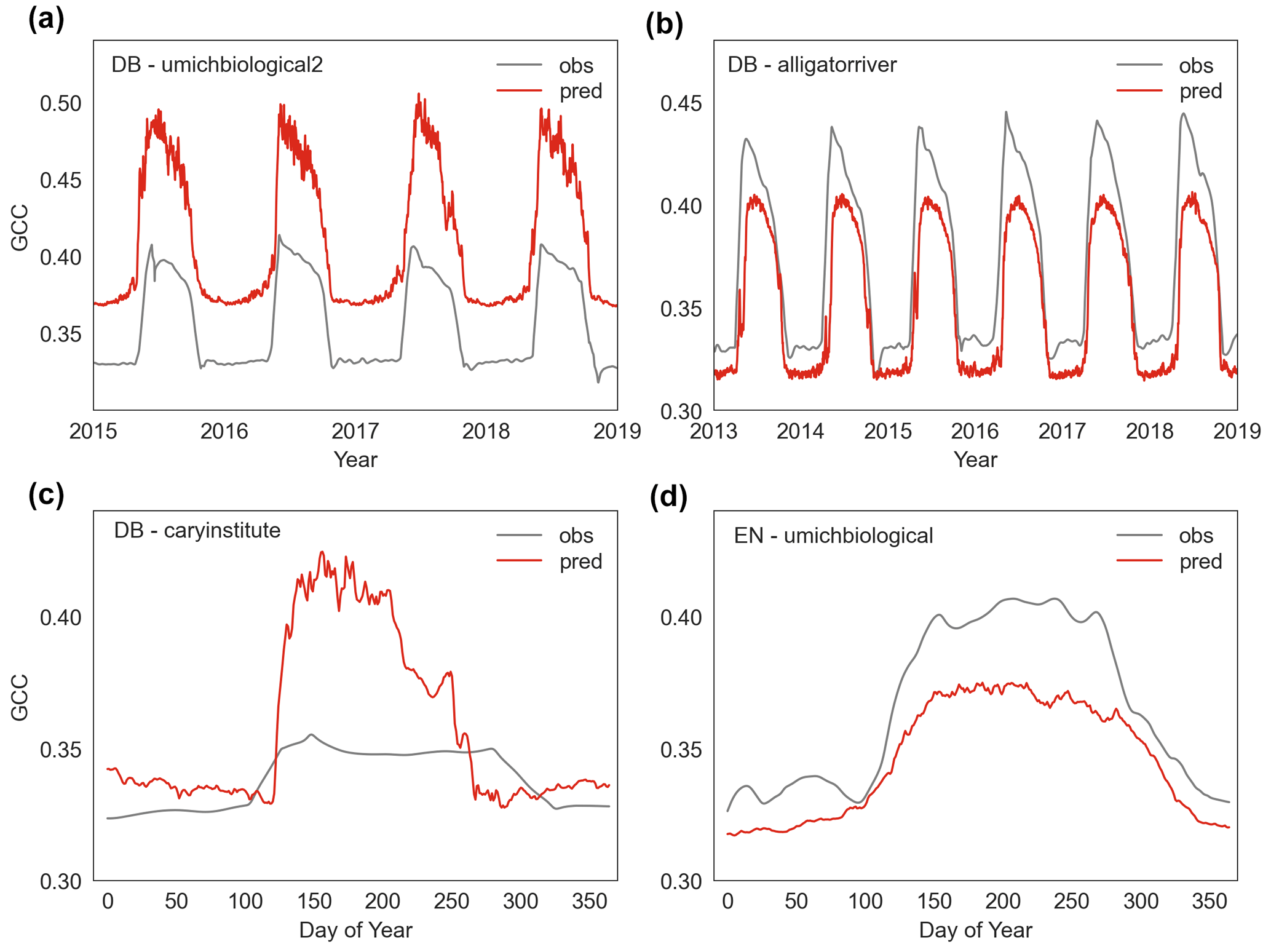
Figure 9 The overestimated and underestimated canopy greenness (GCC) by the LSTM model at some sites (umichbiological2, alligatorriver, caryinstitute, umichbiological) for deciduous broadleaf (DB) and evergreen needleleaf (EN).

The modelling results of vegetation phenology reveal that the full-memory-effect LSTM model is also capable of predicting the shift in phenological transition dates (advance or delay of start of season (SOS) and end of season (EOS)) in most years in the unseen dataset (Fig. 7). The ability to predict the advancement or delay in phenology is crucial for estimating other key processes in the ecosystem functioning, such as ecosystem productivity, as the advancement of spring phenology and the delay of autumn phenology are typically associated with higher productivity (Richardson et al., 2010). Overall, our model's skill to accurately predict the average advance or delay in phenology is encouraging, although it remains challenging to predict the exact phenological dates given the potential and systematic overestimation or underestimation in the GCC cycle (Fig. S4).

4.3 Can the deep learning model of vegetation phenology learn physically plausible relationships?

The sensitivity analysis of our deep learning model sheds light on its ability to learn meaningful physical insights. The model responds to warmer temperatures by predicting an earlier spring onset and later autumn senescence, which is in line with findings from other studies (Menzel et al., 2006; Jeong, 2020). These results underscore the capability of our deep learning framework to reproduce the sensitivity of canopy greenness and phenology to temperature. Our current study primarily focuses on developing the deep learning model. We also conduct a basic sensitivity analysis that has the potential to dismantle the LSTM model and learn from the identified relationship in the data how the response patterns evolve under different climatic conditions. A more extensive and comprehensive sensitivity analyses of the LSTM model, as well as interventional experiments, could offer insights into understanding phenology by identifying which predictors are influential and when. Especially, such approach might help to uncover the control of autumn phenology and its modelling – a long-standing challenge faced by process-based models that may struggle due to inadequate predictors inclusion or response functions (Delpierre et al., 2009; Liu et al., 2019). Moreover, the hybrid models by the integration of physic knowledge into the deep learning models might enhance our understanding of how climate change impacts phenology and associated consequences for the ecosystem, another key challenge in phenology modelling. In numerous Earth system models, such as CLM 4.5 and LPJ (Peano et al., 2021), phenology is modelled based solely on climatic drivers, employing PFT-specific thresholds for factors like chilling and growing degree days. Some models also integrate a more realistic connection to the carbon cycle, where leaf growth incurs a carbon cost. For the phenology representation strictly from climate variables in ESMs, our data-driven approach can serve as a direct replacement for traditional empirical formulations. However, for ESMs that consider phenology to be dependent on available carbon resources, it becomes necessary to allow our data-driven method to evolve into a hybrid model (e.g. ElGhawi et al., 2023, for land–atmosphere fluxes) that also accounts for carbon resources in its inputs and loss function. This entails modelling leaf growth as depleting carbon from the reserve pool and adding dropped leaves to the humus pool, thereby ensuring carbon mass balance. Consequently, carbon mass balance serves as a critical constraint for the data-driven phenology model.

5 Conclusions

In this study, we develop a novel deep learning modelling framework incorporating multiple meteorological memory effects to predict the whole seasonal trajectory of canopy greenness and transition dates for each plant functional type using LSTM. Our key findings can be summarized as follows:

1. The general deep learning model, trained for each PFT using LSTM, demonstrates the ability to generalize to unseen sites, indicating that the deep learning approach effectively captures the underlying mechanics of canopy greenness development.

2. The incorporation of multi-variate meteorological memory effects proves crucial in canopy greenness modelling. The LSTM model, accounting for these memory effects, can reproduce general temporal dynamics of canopy greenness across various timescales, from daily to interannual variability. Furthermore, it captures phenological shift directions, enhancing the model's comprehensive representation.

3. Our sensitivity analysis demonstrates the LSTM model's capability to learn plausible relationships, revealing its proficiency in acquiring fundamental physical knowledge about vegetation greenness and phenological development.

Our deep learning model accounting for multi-variate memory effects holds promise for improving our understanding of vegetation responses to climatic variability. In future, the integration of deep learning phenology models into coupled land surface and Earth system models may further enhance our ability to comprehend and simulate complex interactions and feedback within these systems.