HyPhAICC v1.0: a hybrid physics–AI approach for probability fields advection shown through an application to cloud cover nowcasting

This work proposes a hybrid approach that combines physics and artificial intelligence (AI) for cloud cover nowcasting. It addresses the limitations of traditional deep-learning methods in producing realistic and physically consistent results that can generalise to unseen data. The proposed approach, named HyPhAICC, enforces a physical behaviour. In the first model, denoted as HyPhAICC-1, a multi-level advection dynamics is considered a hard constraint for a trained U-Net model. Our experiments show that the hybrid formulation outperforms not only traditional deep-learning methods but also the EUMETSAT Extrapolated Imagery model (EXIM) in terms of both qualitative and quantitative results. In particular, we illustrate that the hybrid model preserves more details and achieves higher scores based on similarity metrics in comparison to U-Net. Remarkably, these improvements are achieved while using only one-third of the data required by the other models. Another model, denoted as HyPhAICC-2, adds a source term to the advection equation, it impaired the visual rendering but displayed the best performance in terms of accuracy. These results suggest that the proposed hybrid physics–AI architecture provides a promising solution to overcome the limitations of classical AI methods and contributes to open up new possibilities for combining physical knowledge with deep-learning models.

1 Introduction

Meteorological services are responsible for providing accurate and timely weather forecasts and warnings to ensure public safety and mitigate damage to property caused by severe weather events. Traditionally, these forecasts have been based on numerical weather prediction (NWP) models, which provide predictions of atmospheric variables such as temperature, humidity, and wind speed. However, NWP models have inherent limitations in their ability to capture small-scale weather phenomena such as thunderstorms, tornadoes, and localised heavy-rainfall events (Schultz et al., 2021; Matte et al., 2022; Joe et al., 2022).

To address this limitation, the concept of nowcasting has emerged as a valuable tool in meteorology (Lin et al., 2005; Sun et al., 2014). Nowcasting refers to the process of using recently acquired high-resolution observations to generate short-term forecasts of weather conditions, typically on a timescale of minutes to a few hours. Nowcasting techniques exploit various observational data sources, including radar, satellite, lightning, and ground-based observations, to generate real-time estimates of weather conditions and can take advantage of these recent data to significantly outperform NWP on short lead times (Lin et al., 2005; Sun et al., 2014).

Cloud cover nowcasting is a critical component of weather forecasting. It is used to predict the likelihood of precipitation, thunderstorms, and other hazardous weather events. Accurate cloud cover forecasts on a short timescale are particularly important for weather-sensitive applications such as aviation, agriculture, and renewable energy production.

Traditionally, cloud cover forecasting has been done using physics-based methods, relying on the laws of physics to model the evolution of cloud cover, e.g. cloud motion vectors as in Bechini and Chandrasekar (2017) and García-Pereda et al. (2019), optical flow (Wood-Bradley et al., 2012), or NWP-based data assimilation (Ballard et al., 2016). However, with the recent advances in artificial intelligence (AI) and machine learning (ML), data-driven methods have become increasingly popular for these types of tasks (e.g. Espeholt et al., 2022; Ravuri et al., 2021; Trebing et al., 2021; Ayzel et al., 2020; Berthomier et al., 2020; Shi et al., 2015).

Among these data-driven methods, long short-term memory (LSTM) networks, introduced by Hochreiter and Schmidhuber (1997), stand out. LSTMs are a type of recurrent neural network capable of learning long-term dependencies; they are useful for time series predictions, as they can learn from past entries to predict future values. In tasks involving multidimensional data, they are commonly used with convolutional layers, forming what is known as a convolutional LSTM. This neural architecture excels in capturing spatio-temporal correlations compared to fully connected LSTMs (Shi et al., 2015). Spatio-temporal LSTM (Wang et al., 2018) increases the number of memory connections within the network, allowing efficient flow of spatial information. This model was further optimised by adding stacked memory modules (Wang et al., 2019). U-Net is another popular architecture; it was originally designed by Ronneberger et al. (2015) for biomedical image segmentation. Unlike LSTMs, U-Net has no explicit memory modelling, yet it has shown good performance for a binary cloud cover nowcasting task as shown in Berthomier et al. (2020). Furthermore, it has found application in precipitation nowcasting, as highlighted by Ayzel et al. (2020), and a modified version was used for a similar task in Trebing et al. (2021).

Machine learning models hold great promise for addressing scientific challenges associated with processes that cannot be fully simulated due to either a lack of resources or the complexity of the physical process. However, their application in scientific domains faced challenges, including constraints related to large data needs, difficulty in generating physically coherent outcomes, limited generalisability, and issues related to explainability (Karpatne et al., 2017). To overcome these challenges, incorporating physics into ML models is of paramount importance. It leverages the inherent structure and principles of physical laws to improve the interpretability of the model, handle limited labelled data, ensure consistency with known scientific principles during optimisation, and ultimately improve the overall performance and applicability of the models, making them more likely to be generalisable to out-of-sample scenarios. As discussed by Willard et al. (2022) and Cheng et al. (2023), the available hybridisation techniques leverage different aspects of ML models, e.g. the cost function, the design of the architecture, or the weights' initialisation.

A common method to ensure the consistency of ML models with physical laws is to embed physical constraints within the loss function (Karpatne et al., 2017). This involves incorporating a physics-based term weighted by a hyperparameter, alongside the supervised error term. This addition enhances prediction accuracy and accommodates unlabelled data. It has proven to be effective in addressing a range of problems, including uncertainty quantification, parameterisation, and inverse problems (Daw et al., 2021; Jia et al., 2019; Raissi et al., 2019). However, one drawback lies in the challenge of appropriately tuning the hyperparameter.

Given the necessity for an initial choice of model parameters in many ML models, researchers explore ways to inform the initial state of a model with physical insights. One possible way is transfer learning, where a pre-trained model is fine-tuned with limited data (Jia et al., 2021). Additionally, simulated data from physics-based models can be employed for pre-training, akin to methods used in computer vision. This technique has found application in diverse fields, including biophysics (Sultan et al., 2018), temperature modelling (Jia et al., 2019), and autonomous vehicle training (Shah et al., 2017). However, this method requires the assumption that the underlying physics of the simulated data aligns with the real-world data.

To address imperfections in physics-based models, a common strategy is error modelling. Here, an ML model learns to predict the errors (also called residuals) made by the physics-based model (Forssell and Lindskog, 1997). This approach leverages learned biases to correct predictions (see Fig. 1).

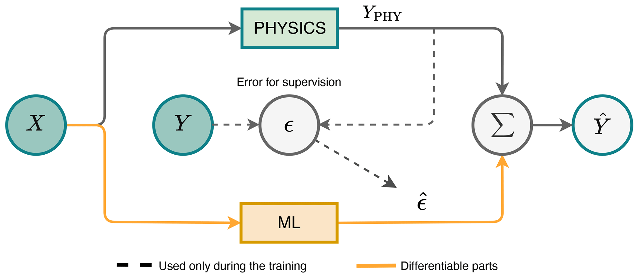
Figure 1 Illustration of error modelling. The physics-based model is used to predict the output, and the ML model is used to predict the residuals. Adapted from Forssell and Lindskog (1997).

A more general approach that does not deal only with errors is to create hybrid models merging physics-based models and ML models. For example, in scenarios where the dynamics of physics are fully defined, the output of a physics-based model can be used as input to an ML model. This approach has demonstrated enhanced predictions in tasks such as lake temperature modelling (Daw et al., 2021). However, in cases where a physical model contains unknown elements requiring coupling with an ML model for joint resolution, a viable strategy involves substituting a segment of a comprehensive physics-based model with a neural network. An illustrative example is found in sea surface temperature prediction, where de Bezenac et al. (2018) employed a neural network to estimate the motion field. In alignment with this strategy, our study proposes leveraging physical knowledge based on the advection equation to address the cloud cover nowcasting task. This results in simulating the advection of clouds by winds while using a neural network to estimate unknown variables, such as the two components of the velocity field.

Moreover, our study introduces an additional requirement, cloud type classification. Specifically, our dataset contains cloud cover observations with pre-existing categorical classifications based on cloud types (e.g. very low clouds, low clouds). This necessitates adopting a probabilistic approach in our hybrid architecture, which, to the best of our knowledge, has not been explored in geophysics. Indeed, adopting a probabilistic approach with probability maps allows us to account for the inherent variability and uncertainties associated with the model's predictions. This also provides a more natural framework for such a classification problem for further extensions of the modelling beyond the advection.

Rather than using the theoretical solution of the equation as proposed in de Bezenac et al. (2018), our hybrid approach solves a system of partial differential equations (PDEs) within a neural network, which makes the architecture more flexible. However, it poses some implementation challenges, as explained in Appendix B. This paper is organised as follows. Section 2 introduces the hybrid architecture. Section 3 is dedicated to presenting results and performance analysis compared to state-of-the-art models. Finally, in Sect. 4, we draw conclusions based on our findings.

2 Methodology

In this work, we address applications involving dynamics with unknown variables that require estimation. For example, the cloud motion field is one of the unknown variables in the application considered. In such cases, as discussed in Sect. 1, a joint resolution approach is more appropriate. Here, the physical model utilises the neural network outputs to compute predictions, integrating the two models as follows:

$$y=\mathit{\varphi }\circ f_{\mathit{\theta }}\left(x\right),$$

where x is the input, f_θ represents the neural network, ϕ denotes the physical model, and y is the output. In this setup, ϕ implicitly imposes a hard constraint on the outputs, potentially accelerating the convergence of the neural network during training.

This method raises some trainability challenges as the physics-based model is involved in the training process, and it should be differentiable, in the sense of automatic differentiation, in order to allow the back-propagation of gradients (refer to Appendix B). We show in Appendix B how spatial derivatives of PDEs can be approximated within a neural network in a differentiable way using convolution operations. This allows us to compute gradients and back-propagate them during the training process. This fundamental knowledge serves as a foundation for our investigation of novel hybrid physics–AI architectures. With these established principles, we present in this section the proposed hybrid architecture, which is applied to cloud cover nowcasting.

In this section, we introduce our hybrid physics–AI architecture, detailed in Sect. 2.1. Section 2.2 explains the different physical modelling approaches investigated in this study. Following that, Sect. 2.3, 2.4, and 2.5 present the training procedure, evaluation metrics, and benchmarking procedure, respectively.

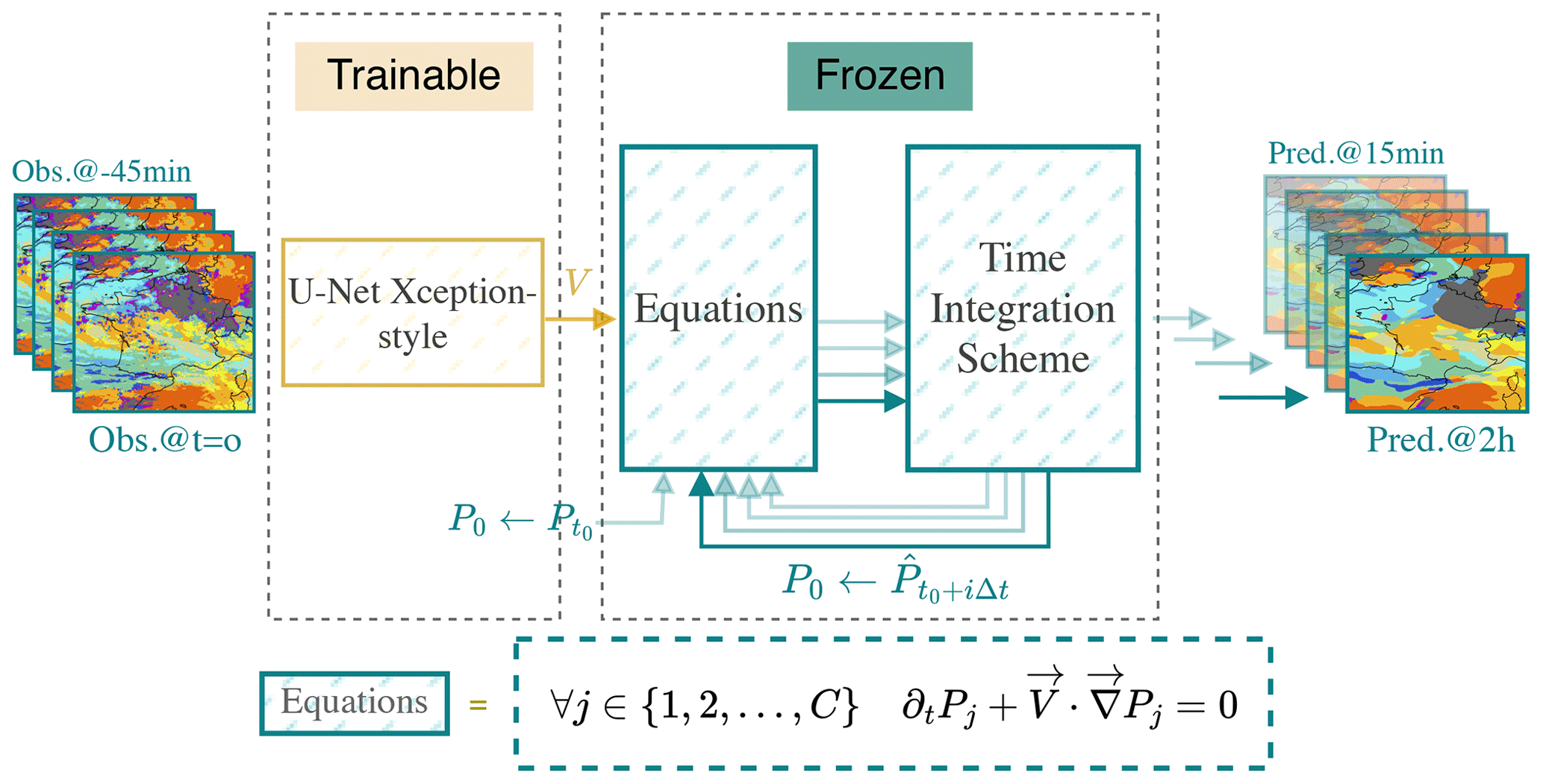
Figure 2 HyPhAICC-1. The proposed hybrid model consists of a U-Net Xception-style model to estimate the velocity field from the last observations; the estimated velocity field is smoothed using a Gaussian filter. The equation is numerically integrated using the fourth-order Runge–Kutta method over multiple time steps. The initial condition (f₀) is updated after each time step to the current state, allowing the computation of the next state.

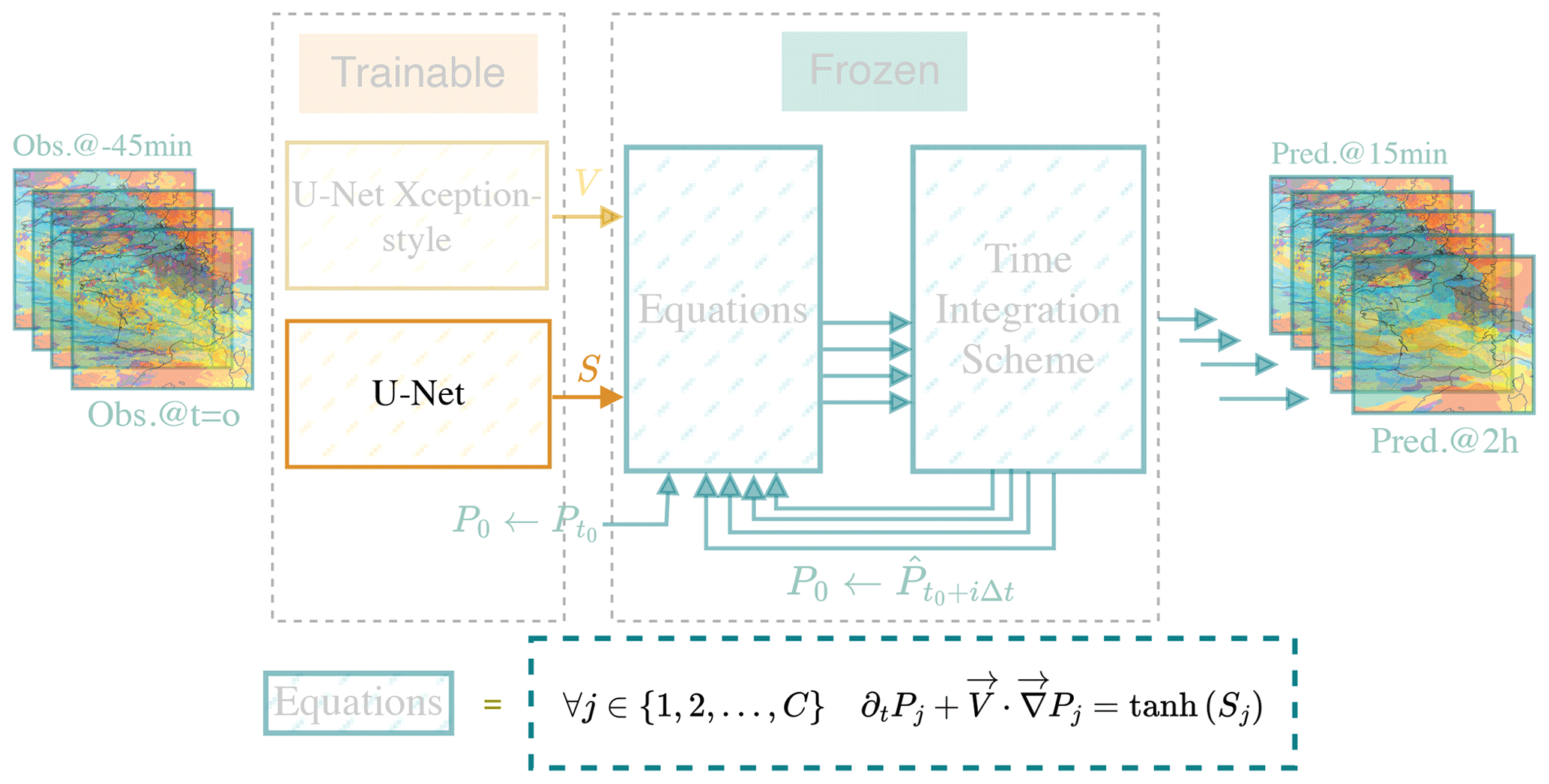
Figure 3 HyPhAICC-2. The second version of the proposed hybrid model. It consists of a U-Net Xception-style model to estimate the velocity field and a second U-Net model to estimate the source term from the last observations. We highlighted the additional parts compared to Fig. 2 and faded the unchanged ones.

2.1 The HyPhAICC architecture

The proposed hybrid architecture is a dual-component system (see Fig. 2). The first component is composed of one or more classical deep-learning models. These models process the most recent observations, yielding predictions for the physical unknowns of interest. The second block takes as inputs the physical variables, whether known or predicted by the neural networks, along with initial conditions. This second component time integrates one or multiple PDEs to generate the subsequent state of the system. The fourth-order Runge–Kutta (RK4) method is used for time integration. These PDEs encode essential physical knowledge. As discussed in the Appendix B4, the spatial derivatives are approximated using convolutional layers.

The parameters of the first component are trainable; they are optimised during training to estimate the unknown variables. However, we froze the parameters of the second block, as it represents already-known operations. This ensures that the second block maintains its fixed structure, representing the known physical knowledge encoded in the equations, while the trainable block focusses on learning and predicting the unknown aspects of the system. This architecture combines the physical knowledge encoded in the equations with the pattern extraction capabilities of neural networks.

In the following, we employ this architecture for cloud cover nowcasting, with different models being implemented, each using a different physical modelling approach.

2.2 Physical modelling

Before delving into the details of the proposed models, let us first establish the essential characteristics of the data at hand. In this work, we investigate cloud cover nowcasting over France using cloud cover satellite images captured by the Meteosat Second Generation (MSG) satellite at 0° longitude. The spatial resolution of the data over France is ≈4.5 km and the time step is 15 min, and each image is of size 256×256. These images have been processed by EUMETSAT (García-Pereda et al., 2019), classifying each pixel into 16 distinct categories. We only considered cloud-related categories, 12 in total.

In what follows, we introduce two models: HyPhAICC-1 which uses an advection equation to capture the motion of clouds, and HyPhAICC-2 which extends this by incorporating a simple source term in the advection equation.

2.2.1 Advection equation: HyPhAICC-1

To easily model the advection of these maps with different cloud types, we adopt a probabilistic approach; i.e. rather than representing a single map showing assigned labels, we use 12 maps, each representing the likelihood or probability of a specific cloud type being present at a given location. These maps must satisfy the following properties.

1. Non-negativity. $P(\mathbf{x},t)\ge \mathrm{0}$ for all x and t, with $\mathbf{x}=(x,y)$, which ensures that the probabilities remain non-negative.

2. Bound preservation. $P(\mathbf{x},t)\le \mathrm{1}$ for all x and t, which ensures that no probability exceeds 1.

3. Probability conservation. ${\sum }_{i=\mathrm{1}}^C{P}_X^i(\mathbf{x},t)=\mathrm{1}$ for all x and t, with C=12 being the total number of cloud types. This property guarantees that the sum of all probabilities is equal to 1.

This approach, known as “one-hot encoding”, is more natural to address classification tasks. It involves using 12 distinct advection equations, each corresponding to a specific cloud type, as described below:

$$\begin{array}{}\text{(1)}& {\partial }_t{P}_j+\mathit{V}\cdot \mathbf{\nabla }{P}_j=\mathrm{0}\forall j\in \left\{\mathrm{1},\mathrm{2},\mathrm{\dots },C\right\},\end{array}$$

where P_j(x) represents the classification probability of the jth cloud type and V(x) is the velocity field, which has two components, i.e. u(x) and v(x). Finally, ∇ denotes the gradient operator.

Although one might initially perceive similarities between this modelling and a Fokker–Planck equation (Fokker, 1914; Pavliotis and Stuart, 2008, Chap. 6), the modelling approach presented here deviates significantly from the Fokker–Planck equation. In contrast, the Fokker–Planck equation is typically employed to depict the evolution of probability distributions for time-continuous Markov processes over continuous states, e.g. Brownian motion. On the other hand, Eq. (1) characterises the probability advection for each finite state.

Nevertheless, by employing equations in the following form:

$$\begin{array}{}\text{(2)}& {\partial }_t{P}_j+\mathcal{L}\left(P_j\right)=\mathrm{0}\forall j\in \left\{\mathrm{1},\mathrm{2},\mathrm{\dots },C\right\},\end{array}$$

where ℒ represents a differential operator with non-zero positive derivative orders, we demonstrate in Appendix D that the probability conservation property is maintained over time. This assertion holds even in scenarios where the discretisation scheme introduces some diffusion or dispersion effects during the resolution process (see Appendix D2 and Appendix E). However, the non-negativity and bound preservation properties are compromised when a discretisation scheme with dispersion effects is used, unlike the diffusive schemes. Consequently, we opt for the first-order upwind diffusive discretisation scheme (see Appendix E2 for details about the equivalent equation) along with the RK4 for time integration. During the time integration process, we perform the integration by subdividing the time step Δt=1 (representing 15 min) into smaller steps δt=0.1 to satisfy the Courant–Friedrichs–Lewy (CFL) condition (Courant et al., 1928); this condition ensures the stability of the numerical solution.

In the first hybrid model, denoted as HyPhAICC-1, we use a U-Net Xception-style model (Tamvakis et al., 2022) inspired by the Xception architecture (Chollet, 2017). It takes the last four observations stacked on the channel axis and estimates the velocity field (see Fig. 2). This model will be guided during training by the advection equation to learn the cloud motion patterns.

2.2.2 Advection with source term: HyPhAICC-2

As the advection alone does not take into account other physical processes, especially class change, appearance, and disappearance of clouds, we propose adding a trainable source term to capture them. In this first attempt, we use a simple source term:

$$\begin{array}{}\text{(3)}& {\partial }_t{P}_j=\tanh \left(S_j\right)\forall j\in \left\{\mathrm{1},\mathrm{2},\mathrm{\dots },C\right\},\end{array}$$

where S_j is a 2D map. The hyperbolic tangent activation function (tanh) is used to keep the values of the source term in a range of $\left[-\mathrm{1},\mathrm{1}\right]$, preventing it from exploding.

The second version of the hybrid model, denoted as HyPhAICC-2, adds this source term to the advection. This modelling is described in the following equation:

$$\begin{array}{}\text{(4)}& {\partial }_t{P}_j+\mathit{V}\cdot \mathbf{\nabla }{P}_j=\tanh \left(S_j\right)\forall j\in \left\{\mathrm{1},\mathrm{2},\mathrm{\dots },C\right\},\end{array}$$

where S_j is estimated using a second U-Net model (see Fig. 3).

While the previous modelling describes the missing physical process in the advection, it does not satisfy the probability conservation property. Thus, this modelling does not conserve the probabilistic nature of P over time. To ensure the appropriate dynamics of probability, a robust framework is provided by continuous-time Markov processes across finite states (Pavliotis and Stuart, 2008, Chap. 5). In this framework, the probability trend is controlled by linear dynamics, ensuring the bound preservation, positivity, and probability conservation. Two other models based on this framework, named HyPhAICC-3 and HyPhAICC-4, are presented in Appendix A1 and Appendix A2, respectively. However, these models did not show any performance improvement compared to the simpler HyPhAICC-1.

Indeed, beyond the performance aspect, this hybridisation framework is flexible, is not limited to the advection, and can be extended to other physical processes.

2.3 Training procedure

The training was carried out on a dataset containing about 3 years of data from 2017 to 2019, with a total of 105 120 images. The images with zero cloud cover were removed, then we assembled all the sequences with 12 consecutive images. After this cleaning step, we randomly split the dataset, 8224 sequences were used for training, and 432 for validation. The test set was performed on a separate dataset from the same region but from 2021.

To improve the diversity of the training set and take into account a possible overfitting on the typical movements of clouds in the western Europe region, we randomly applied simple transformations to the images. More precisely, we applied rotations of 90, 180, and 270°, which increased the dataset size and improved the model's ability to learn various cloud motion patterns.

PyTorch framework is used to implement the models, and the cross-entropy loss function is employed for training. This function is given by

$$\begin{array}{}\text{(5)}& l(Y,p)=-{\displaystyle \frac{\mathrm{1}}{N}}\sum _{i=\mathrm{1}}^N\sum _{j=\mathrm{1}}^C{Y}_{i,j}\log \left(p_{i,j}\right),\end{array}$$

where N represents the total number of pixels, C denotes the number of classes, p_i,j is the predicted probability of the ith pixel belonging to the jth class, and Y_i corresponds to the one-hot encoded ground truth at the ith pixel, i.e. $Y_{i,j}=\mathrm{0}$, except for the correspondent cloud type, where $Y_{i,j}=\mathrm{1}$.

The training of the model parameters is achieved through gradient-based methods. Here, an Adam optimiser (Kingma and Ba, 2017) is used with a learning rate of 10⁻³ and a batch size of 4 with 16 accumulation steps, allowing us to simulate a batch size of 64. The training was performed using a single Nvidia A100 GPU for 30 epochs.

You can find the source code for our project on GitHub at https://github.com/relmonta/hyphai (last access: 7 June 2024).

2.4 Performance metrics

To evaluate the performance of competing models in this study, we employed various metrics. Firstly, standard classification metrics are used to evaluate the statistical aspect, then the Hausdorff distance is introduced to evaluate the qualitative aspect of the results.

2.4.1 Classic classification metrics

The selected metrics include accuracy, precision, recall, F1 score, and critical success index (CSI, Gilbert, 1884), also called intersection over union (IoU) or Jaccard index. These metrics offer multiple insights into different aspects of model performance. Accuracy measures the proportion of correct predictions, while precision quantifies the proportion of correct positive predictions relative to the total number of positive predictions. Recall evaluates the proportion of correct positive predictions relative to the total number of positive cases. The F1 score provides a balance between precision and recall. The CSI measures the overlap between prediction and ground truth, providing a measure of similarity.

To compute these metrics for the jth class, we use the following formulas:

$$\begin{array}{c}{\displaystyle }{\text{Accuracy}}_j={\displaystyle \frac{{\text{TP}}_j+{\text{TN}}_j}{{\text{TP}}_j+{\text{TN}}_j+{\text{FP}}_j+{\text{FN}}_j}},\\ {\displaystyle }{\text{Recall}}_j={\displaystyle \frac{{\text{TP}}_j}{{\text{TP}}_j+{\text{FN}}_j}},\\ {\displaystyle }{\text{Precision}}_j={\displaystyle \frac{{\text{TP}}_j}{{\text{TP}}_j+{\text{FP}}_j}},\\ {\displaystyle }{\text{F1}}_j={\displaystyle \frac{\mathrm{2}\times {\text{Precision}}_j\times {\text{Recall}}_j}{{\text{Precision}}_j+{\text{Recall}}_j}},\\ {\displaystyle }{\text{CSI}}_j={\displaystyle \frac{{\text{TP}}_j}{{\text{TP}}_j+{\text{FP}}_j+{\text{FN}}_j}}.\end{array}$$

These metrics are calculated separately for each class, where TP denotes instances correctly identified as positive cases, TN refers to instances correctly identified as negative cases, FP represents cases misclassified as positives, and FN is the number of positive cases that are classified as negative.

To obtain an overall performance evaluation of the accuracy, we use the following formula:

$$\text{Accuracy}={\displaystyle \frac{{\sum }_j{\text{TP}}_j}{\text{Total number of cases}}}.$$

For the remaining metrics, we can calculate two types of average: the macro-average and the micro-average. The macro-average is the arithmetic mean of the metric scores computed for each class, while the micro-average considers all classes as a single entity (Takahashi et al., 2022). Given the highly imbalanced distribution of labels in our dataset, we adopted the macro-average to evaluate the models' performance (Fernandes et al., 2020; Wang et al., 2021). The macro-averaged F1 is defined as in Sokolova and Lapalme (2009) as follows:

$${\text{F1}}_{\mathrm{macro}}={\displaystyle \frac{\mathrm{2}\times {\text{Precision}}_{\mathrm{macro}}\times {\text{Recall}}_{\mathrm{macro}}}{{\text{Precision}}_{\mathrm{macro}}+{\text{Recall}}_{\mathrm{macro}}}},$$

where the macro-averaged precision and recall are defined as follows:

$$\begin{array}{c}{\displaystyle }{\text{Precision}}_{\mathrm{macro}}={\displaystyle \frac{\mathrm{1}}{C}}\sum _{j=\mathrm{1}}^C{\text{Precision}}_j.\\ {\displaystyle }{\text{Recall}}_{\mathrm{macro}}={\displaystyle \frac{\mathrm{1}}{C}}\sum _{j=\mathrm{1}}^C{\text{Recall}}_j.\end{array}$$

We define the macro-averaged CSI following the same method as follows:

$${\text{CSI}}_{\mathrm{macro}}={\displaystyle \frac{\mathrm{1}}{C}}\sum _{j=\mathrm{1}}^C{\text{CSI}}_j.$$

These pixel-wise metrics are commonly used for evaluating image segmentation tasks or more generally classification tasks, but it is important to note the limitations of these metrics and evaluation approaches. Although selected metrics provide valuable insights, they do not capture all aspects of model performance, for instance, because they do not take into account the spatial correspondence between predicted and ground-truth cloud structures. This means that a model can statistically perform well using pixel-wise metrics but still have poor performance in identifying the correct cloud structures or miss a significant amount of detail. As a result, evaluating cloud cover forecasting models based solely on pixel-wise metrics may not be sufficient to ensure their effectiveness in real-world applications.

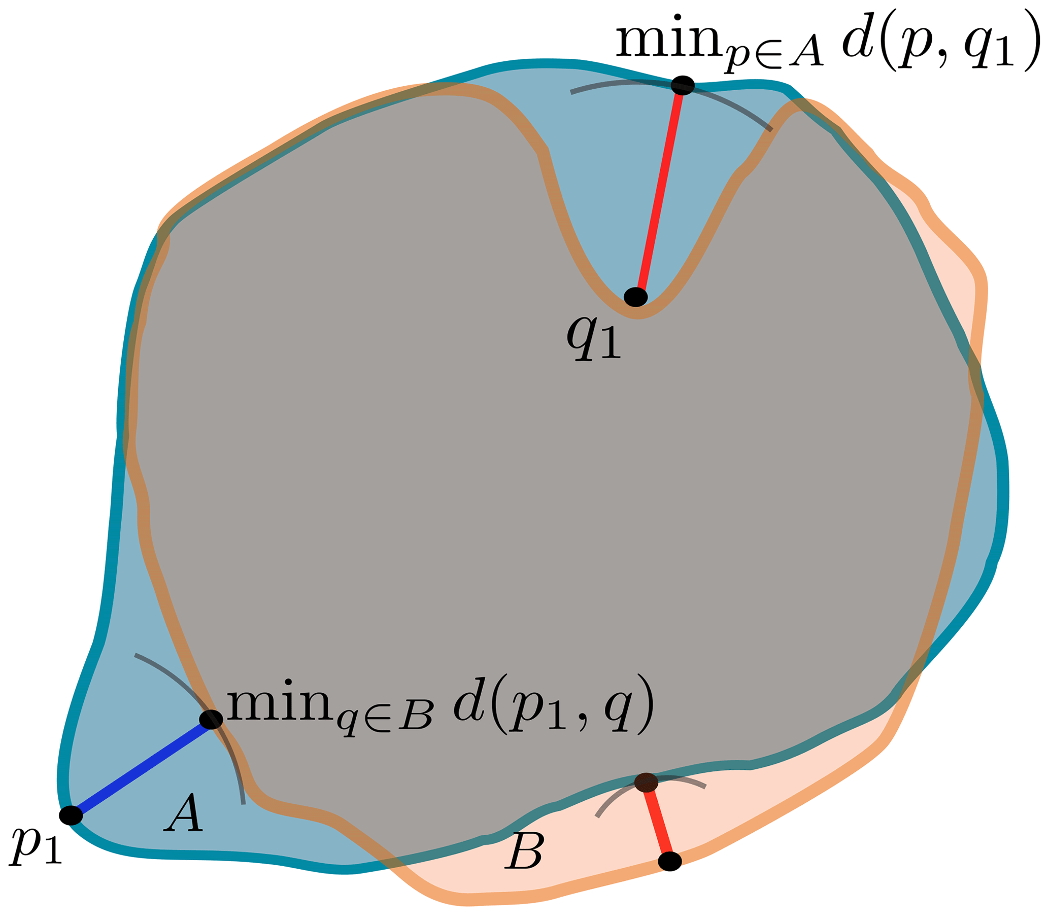
Figure 4 Illustration of the ${min}_{p\in A}d(p,q_{\mathrm{1}})$ and ${min}_{q\in B}d(p_{\mathrm{1}},q)$ quantities used to compute the Hausdorff distance; for each point, we look for the closest point in the other region.

2.4.2 Hausdorff distance

The Hausdorff distance is a widely used metric for medical image segmentation (e.g. Karimi and Salcudean, 2019; Aydin et al., 2021). This metric measures the similarity between the predicted region and the ground-truth region by comparing structures rather than just individual pixels. It can be expressed using either Eq. (6) or Eq. (7), which are described as follows:

$$\begin{array}{}\text{(6)}& {\displaystyle }{h}^{\mathrm{1}}(A,B)={\displaystyle \frac{\mathrm{1}}{\left|A\right|}}\sum _{p\in A}\underset{q\in B}{min}d(p,q),\text{(7)}& {\displaystyle }{h}^{\mathrm{2}}(A,B)=\underset{p\in A}{max}\underset{q\in B}{min}d(p,q),\end{array}$$

where d(p,q) is the Euclidean distance between p and q. The former computes the mean distance between each point A and the closest point in B, providing an overall measure of similarity. The latter measures the maximum distance between a point in A and the closest point in B (Fig. 4), this formulation is a more conservative measure that focuses on the largest discrepancies between the sets. Both formulations exhibit sensitivity to the loss of small structures. Specifically, when small regions in the ground truth are non-empty while their corresponding regions in the prediction are empty, the search area expands, which increases the overall distance. We opt to limit this search region to the maximum distance traversable by a cloud. Consequently, we introduce the restricted Hausdorff distance (rHD), which is defined as follows:

$$\begin{array}{}\text{(8)}& h^{\mathrm{3}}(A,B)={\displaystyle \frac{\mathrm{1}}{\left|A\right|}}\sum _{p\in A}\underset{q\in {\mathbf{B}}_r\left(p\right)}{min}d(p,q),\end{array}$$

where B_r(p) is the ball of radius r centred at p. In our experiments, we set r to 10 pixels, which corresponds to a radius of approximately 45–50 km, corresponding to the maximum distance crossed by clouds in one time step, considering 200 km h⁻¹ as the cloud's maximum speed. This means that for each pixel in the first set, we compute the distance to the closest pixel in the second set, but we only do this if it is within a radius of 10 pixels. This allows us to reduce the impact of small regions in the ground truth that are not present in the prediction, while still rewarding the model if it correctly predicts them.

The Hausdorff distance is a directed metric, i.e. $h^p(A,B)\ne h^p(B,A)$; thus, we consider the maximum of the two directed distances as follows:

$$\begin{array}{}\text{(9)}& \mathcal{H}(S,\widehat{S})=max\left(h^{\mathrm{3}}(S,\widehat{S}),h^{\mathrm{3}}(\widehat{S},S)\right),\end{array}$$

where S and $\widehat{S}$ are the coordinates of positive pixels in the ground truth and prediction, respectively.

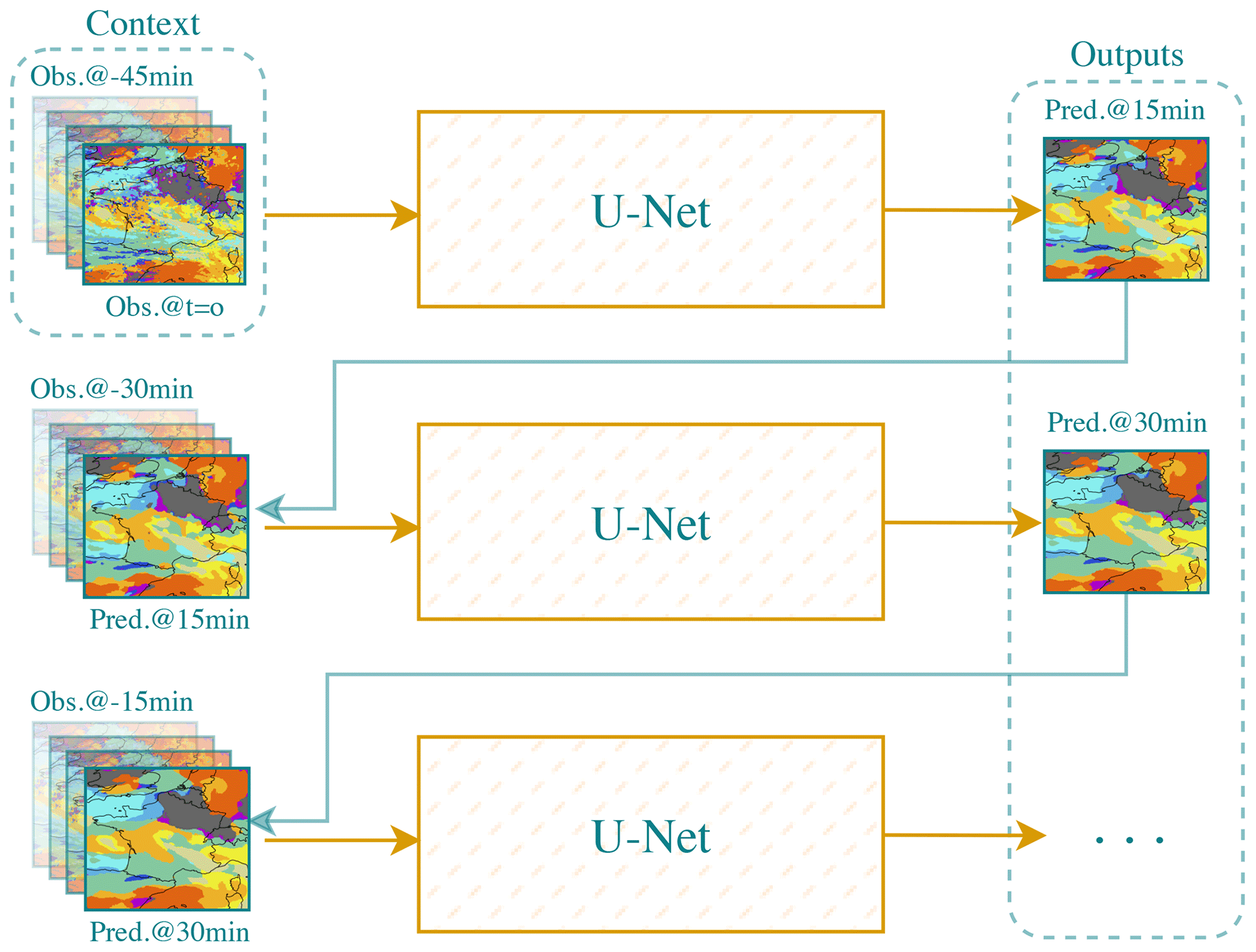
Figure 5 The U-Net architecture considered in the comparison. U-Net is iteratively used to predict the next state given the previous ones.

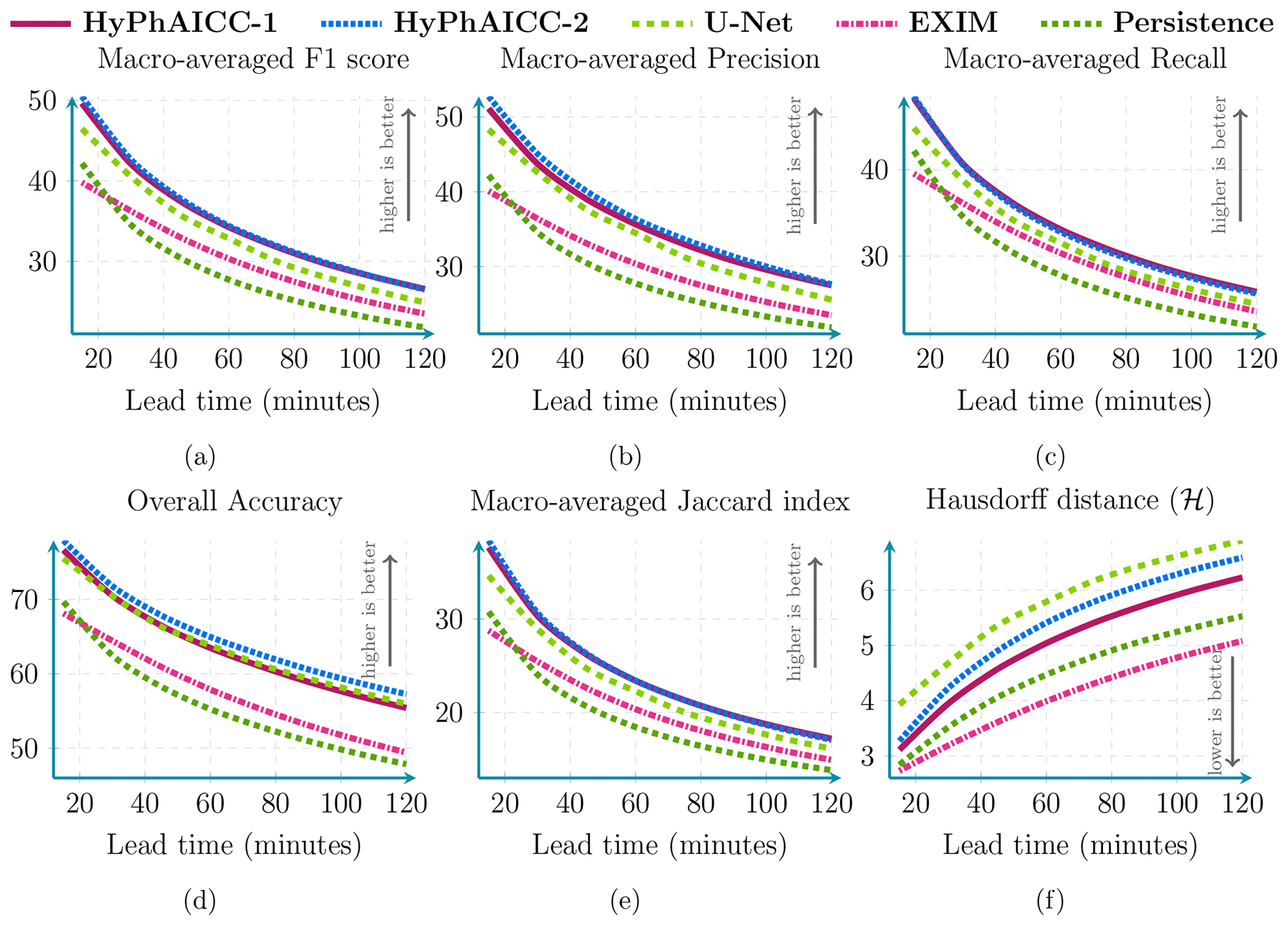
Figure 6 Performance comparison between our HyPhAICC-1, U-Net, EXIM, and the persistence baseline using five metrics: averaged F1 score (%), precision (%), recall (%), accuracy (%), CSI (%), and Hausdorff distance (defined in Eq. 9). These scores were computed over 1000 random samples covering France in 2021. See Fig. A3 for confidence intervals.

2.5 Benchmarking procedure

To assess the performance of the proposed models, we consider established benchmarks. In the comparative evaluation, we included the well-known U-Net (Ronneberger et al., 2015). This classical U-Net is different from the one used to estimate the velocity in the proposed hybrid models (refer to Figs. 2 and 3). The choice of this classical U-Net for comparison is justified by the fact that it is the most widely used in the literature for the same task (e.g. Ayzel et al., 2020; Berthomier et al., 2020; Trebing et al., 2021). U-Net architecture is structured with a contracting path and an expansive path connected by a bottleneck layer. The contracting path comprises four levels of convolutional layers, each followed by a max pooling layer. The number of filters we used in these convolutional layers progressively increases from 32 to 64, 128, and finally 256. On the other hand, the expansive path consists of four sets of convolutional layers, each followed by an upsampling layer. These layers help in the reconstruction and expansion of the feature maps to match the original input size. We iterate over U-Net, as illustrated in Fig. 5, to generate predictions for multiple future time steps.

In addition to U-Net, we consider in our comparison a product called EXIM (for extrapolated imagery), developed by EUMETSAT as part of their NWCSAF/GEO products (García-Pereda et al., 2019). This product involves applying the atmospheric motion vector field multiple times to a current image to produce forecasts. Each pixel's new location is calculated using the motion vector, and this process is repeated assuming a constant displacement field. For continuous variables like brightness temperature, the method uses weighted contributions to forecast pixel values, ensuring that there are no gaps by interpolating values from adjacent pixels if necessary. For categorical variables such as cloud type, the pixel value is directly assigned to the new location, and conflicts are resolved by overwriting. If a pixel is not touched by any trajectory, the value is determined by the majority class of its nearest neighbours (García-Pereda et al., 2019) (https://www.nwcsaf.org/exim_description, last access: 4 July 2024). This approach is also called kinematic extrapolation.

We also included a commonly used meteorological baseline method known as “persistence”. This method predicts future time steps by simply using the last observation, a relevant approach in nowcasting since weather changes occur slowly, making the last observation a strong prediction, which makes the persistence baseline challenging to outperform.

We tested the competing models using 1000 satellite images samples captured over France from January 2021 to October 2021.

Table 1 Score comparison at the 120 min lead time (↑: higher is better; ↓: lower is better). The best scores are indicated in bold font.

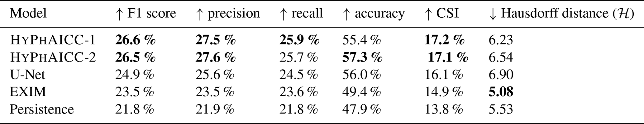
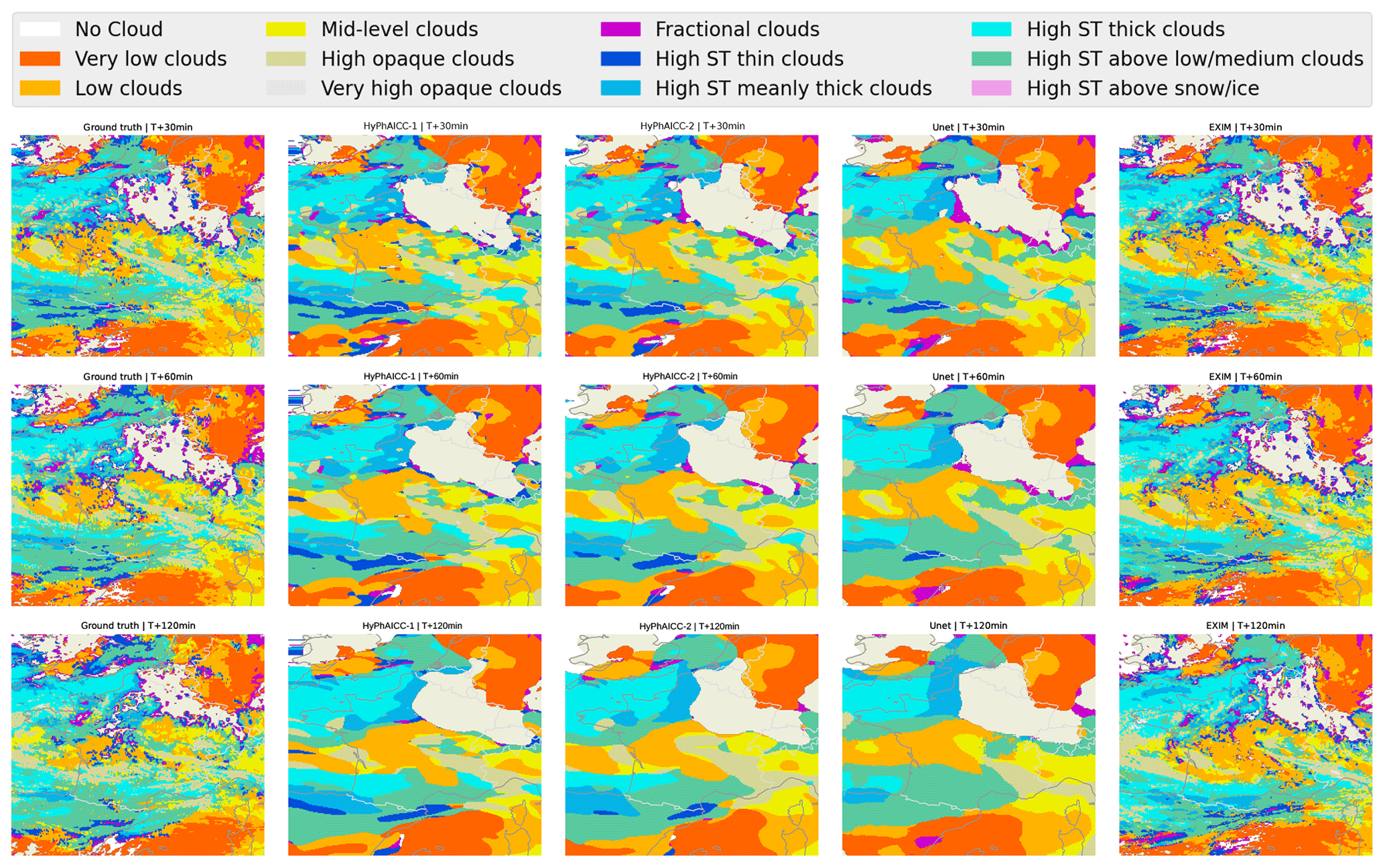
Figure 7 Case study of different models' forecasts. The left column shows ground truth at different time steps. The middle columns show, from left to right, HyPhAICC-1, HyPhAICC-2, and the U-Net predictions, respectively. The right column shows EXIM's predictions. The light beige colour corresponds to the land areas, and the “ST” abbreviation in the legend stands for “semi-transparent”.

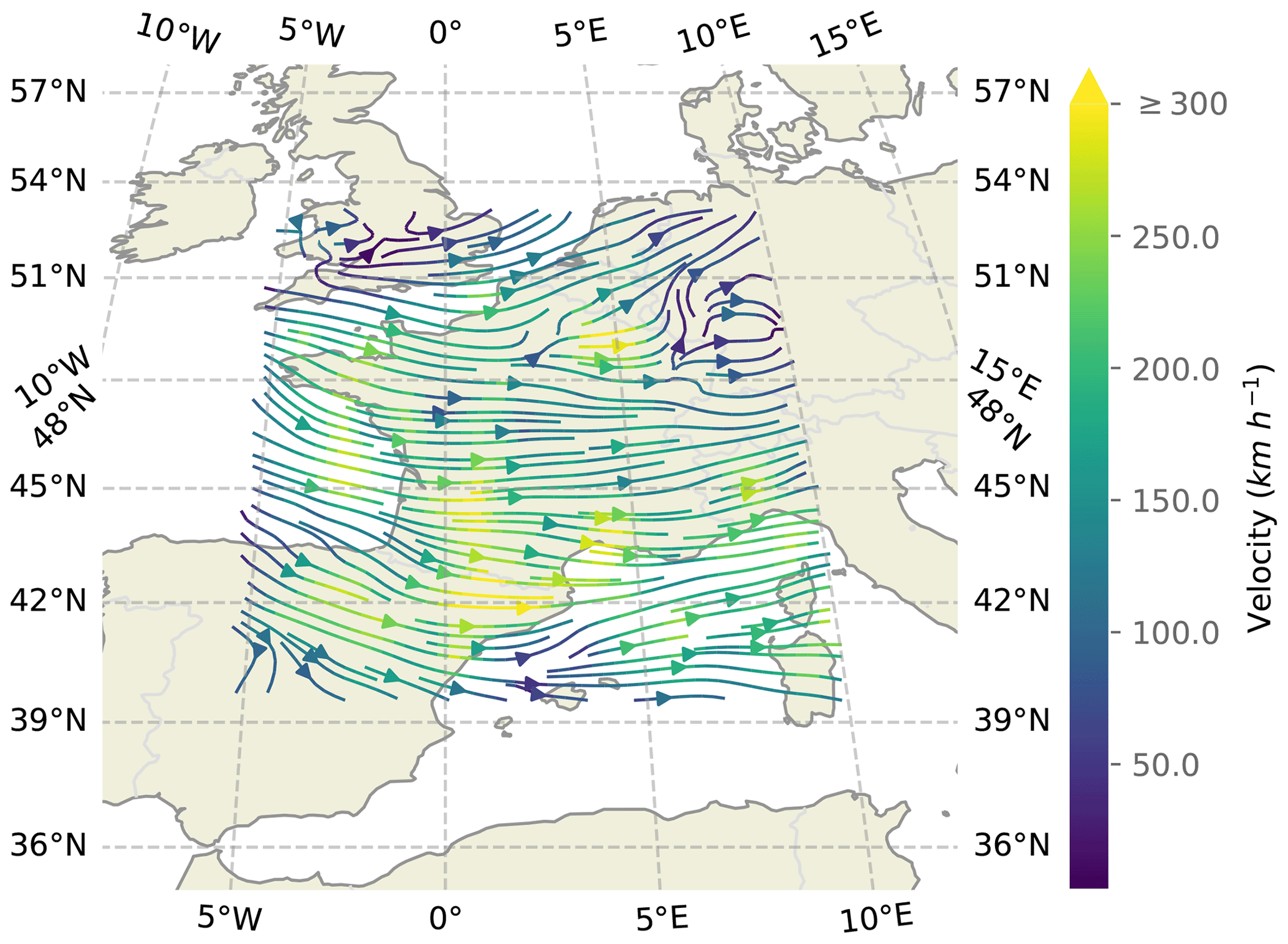
Figure 8 Estimated velocity field by the U-Net Xception-style architecture used in the HyPhAICC-1 model.

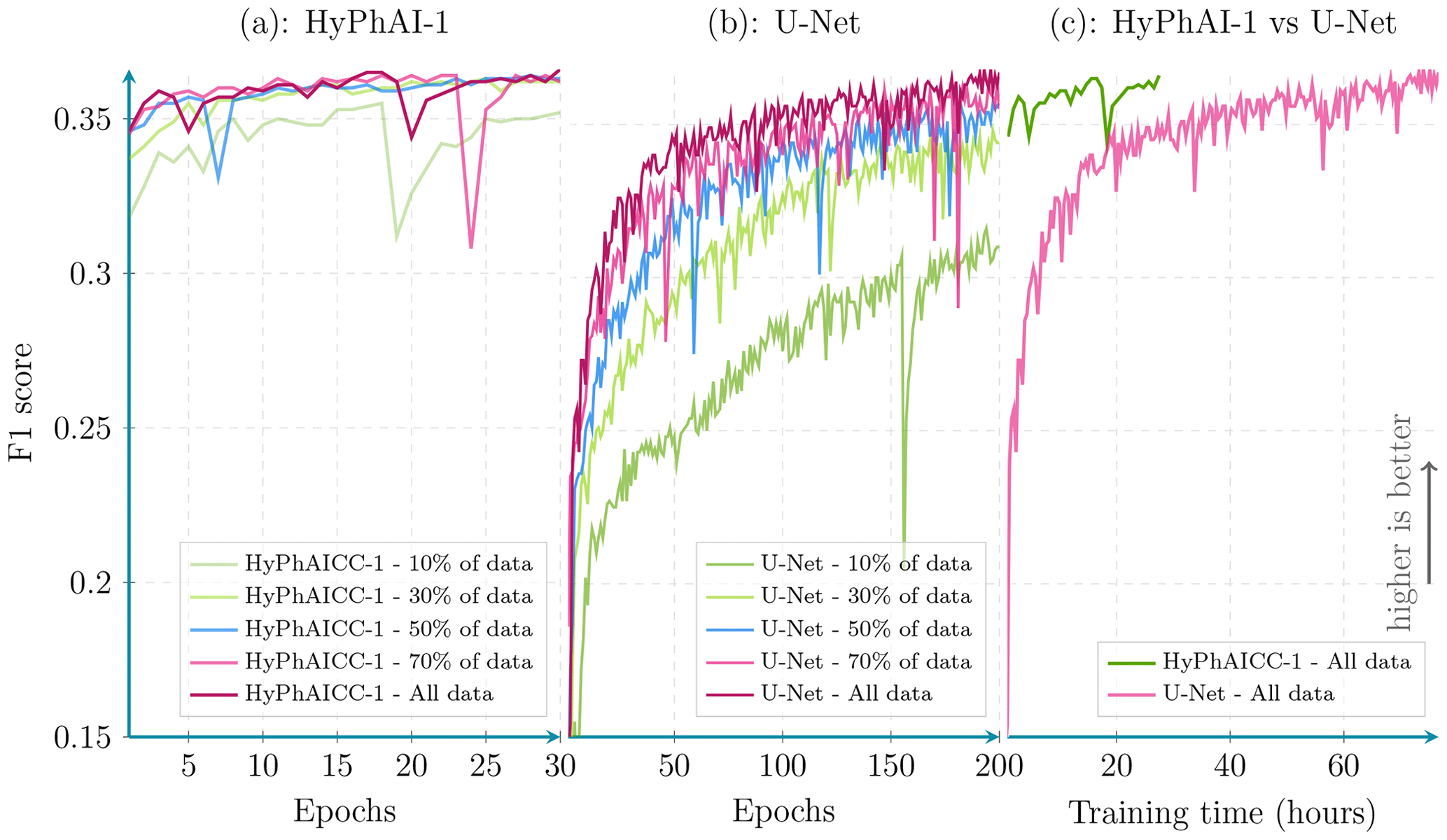
Figure 9 Per epoch validation F1 score comparison between HyPhAICC-1 and U-Net. Scores were calculated from 100 random samples covering France (averaged over all lead times).

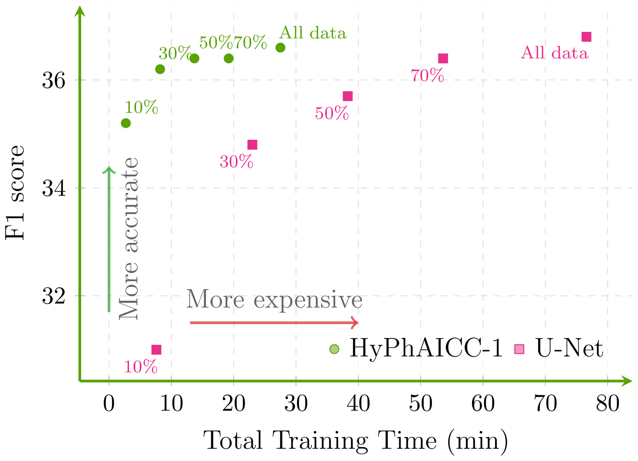
Figure 10 Total training time and maximum validation F1 scores over the last five epochs for U-Net and HyPhAICC-1 using different training data sizes (averaged over all lead times).

3 Experiments and results

We trained the hybrid models, in addition to the U-Net model used for comparison, on 3 years of data. The models were designed to predict a 2 h forecast at 15 min intervals.

3.1 Quantitative analysis

Diving into the numerical evaluations, here we present a comparative analysis based on standard metrics used in image classification tasks. Figure 6 shows a score comparison using different metrics over multiple lead times up to 2 h. The confidence intervals, indicating statistical significance, are computed using a resampling method called bootstrap, which is a statistical technique that involves repeatedly sampling from a single dataset to generate numerous simulated samples (Efron, 1979). Through this method, standard errors, confidence intervals, and hypothesis testing can be computed. Table 1 and Fig. 6 show that HyPhAICC-2 is slightly better in terms of precision and accuracy than the model using advection equation without source term (HyPhAICC-1), and both of these hybrid models significantly outperform the U-Net model in terms of F1 score, precision, and CSI and perform similarly in terms of accuracy and recall. This is because the U-Net model tends to give more weight to the dominant classes at the expense of the other classes, resulting in a higher false positive rate.

Although quantitative performance metrics offer a numerical assessment of a model's ability to predict weather states, providing crucial insights into the reliability and precision of forecasts, they are not sufficient on their own. Qualitative aspects also play a significant role, including the visual interpretation of model predictions and an assessment of its capability to capture complex atmospheric patterns and phenomena.

3.2 Qualitative analysis

Figure 7 presents a case study involving multiple models, highlighting that HyPhAICC-1 produces more realistic and less blurry forecasts compared to the U-Net model. To substantiate this claim, we used the restricted Hausdorff distance (rHD), described in Eq. (8), to assess the sharpness of predicted cloud boundaries. Both HyPhAICC-1 and HyPhAICC-2 models outperformed the U-Net model in this metric, as shown in Fig. 6. EXIM and the persistence baseline exhibit superior results in terms of the Hausdorff metric, and the gap between them and the other models increases with the lead time, which is visually expected. The reason behind this result is that the hybrid models, especially HyPhAICC-1, preserve more details compared to the U-Net model. The lost details in HyPhAICC-1's predictions are only due to the numerical scheme. In ideal conditions, HyPhAICC-1 should preserve the same details during the advection process, and there is no other trainable part in between that can smooth the predictions; however, the upwind discretisation used a scheme that adds a numerical diffusion and crushing the small cloud cells (refer to Appendix E for more details). In contrast, U-Net focuses more on dominant structures and labels, which are more likely to persist over time, which is statistically relevant. Nevertheless, EXIM and the persistence baseline still outperform the other models in this regard. This observation aligns with the fact that the persistence uses the last observation as its predictions, and EXIM is advecting the last observation using the kinematic extrapolation, which keeps the same level of details without diffusion effects (García-Pereda et al., 2019). However, EXIM is slightly more accurate, compared to persistence, in terms of predicted cloud positions.

In Fig. 8, we present the estimated velocity field generated by the HyPhAICC-1 model, illustrated in Fig. 2. This field exhibits a high level of coherence with the observed cloud cover displacements, with exceptions in cloud-free areas, as expected. It is important to emphasise that this velocity field is derived exclusively from cloud cover images, without relying on external wind data or similar sources. This aspect adds a layer of interest, especially in the context of other applications beyond the cloud cover nowcasting.

3.3 Time efficiency

In what follows, we focus only on the HyPhAICC-1 model. By including physical constraints into these hybrid models, we expect a decrease in training time compared to that of the U-Net model. Indeed, Fig. 9 illustrates the evolution of the validation F1 score for both the U-Net and HyPhAICC-1 models across epochs. HyPhAICC-1 converges faster than U-Net. Its convergence does indeed occur after just about 10–15 epochs. Each epoch of the HyPhAICC-1 training takes approximately 55 min using a single Nvidia A100 GPU, while the entire training over 30 epochs takes 27 h. On the other hand, U-Net necessitates up to 200 epochs for achieving similar performance, with each epoch taking around 23 min using the same hardware, which corresponds to about 3 d of training. This difference implies that training U-Net is significantly more expensive compared to HyPhAICC-1.

In inference mode, the hybrid models and U-Net generate predictions within a few seconds, while EXIM's predictions are produced within 20 min (Berthomier et al., 2020), which is one of the main drawbacks of this product.

3.4 Data efficiency

To delve deeper into the efficiency of the proposed HyPhAICC-1 model, we conducted various experiments using different training data sizes. In each experiment, both HyPhAICC-1 and U-Net were trained with 70 %, 50 %, 30 %, and 10 % of the available training data (Figs. 9, 10). Notably, we observed a more significant performance drop for U-Net compared to HyPhAICC-1. Interestingly, the hybrid model exhibited a similar performance using only 30 % of the training data to it when it used the entire dataset (Fig. 9). This finding indicates that this hybrid model is remarkably data efficient, capable of delivering satisfactory performance even with limited training data, which has been highlighted by other studies (Schweidtmann et al., 2024; Cheng et al., 2023). This quality is very important, particularly for tasks with insufficient provided data.

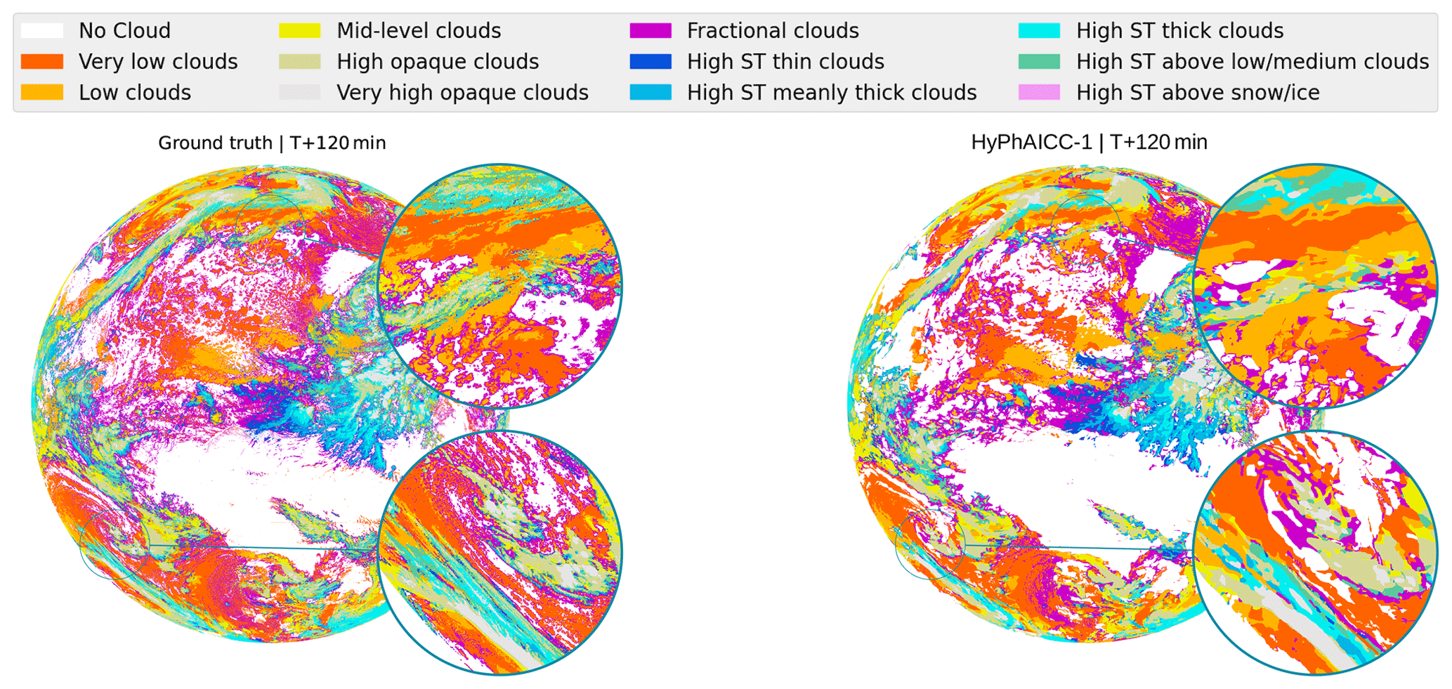
Figure 11 Full-disc cloud cover nowcasting predictions. Zoomed-in views of the 120 min observation and prediction.

3.5 Application to Earth's full disc

To check HyPhAICC-1's capabilities on broader scales after training it on a small region, we tested it on a much larger domain, an entire hemisphere of the Earth – also called a full disc – centred at 0° longitude. The satellite observations of this expansive full-disc domain are of size 3712×3712, which is 210.25 times larger than the size of the training ones. It has diverse meteorological conditions and includes projection deformations when mapped onto a two-dimensional plane, while the extreme deformations at the edge of the disc make this data less useful for operation purposes, it still provides an interesting testing ground for HyPhAICC-1's generalisation ability. In this analysis, we focus only on visual aspects. Despite the significant differences between the training domain and the full disc, we observed good qualitative forecasts of the HyPhAICC-1 model on this new domain without any specific training on it (see Figs. 11 and A4). The cloud motion estimation on the full disc was found to be visually consistent (a Video Supplement is provided at https://doi.org/10.5281/zenodo.10375284, El Montassir et al., 2023b).

This successful transferability of the model highlights its potential robustness and suggests that the underlying principles of cloud motion captured during training are applicable across different domain sizes and different projections (see Appendix C for a formal explanation). Note that the model requires a data size divisible by 2^d, where d is the number of the encoder blocks within the U-Net-Xception model. Indeed, the possibility of running a model using different data sizes is one of the advantages of fully convolutional networks (FCNs) as the convolution operation is independent of the input size.

Overall, HyPhAICC-1 offers an effective and cheaper approach compared to EXIM, with higher efficiency, requiring fewer data compared to U-Net, with the potential to outperform existing models and enable more accurate and efficient weather forecasting. The ability of HyPhAICC-1 to adapt and perform well on the full-disc data, despite being trained on a smaller domain, demonstrates the generalisation capabilities of this hybrid model. This is an important property for weather forecasting models, as it is not always possible to train a model on full-disc data due to the high computational cost.

4 Conclusions

In this study, we introduced a hybrid physics–AI framework that combines the insights from partial differential equations, representing physical knowledge, with the pattern extraction capabilities of neural networks. Our primary focus was on applying this hybrid approach to the task of cloud cover nowcasting, also involving cloud type classification. To leverage continuous physical advection phenomena for this discrete classification task, we proposed a probabilistic modelling strategy based on the advection of probability maps. This flexible approach was easy to adapt to include the prediction of source terms, demonstrating its versatility.

The first model, HyPhAICC-1, leverages the advection equation and slightly outperforms the widely used U-Net model in the quantitative metrics, while showing a significantly better performance in the qualitative aspect. This hybrid model requires a significantly lower amount of data and converges faster, cutting down the training time, which is expected as the physical modelling implicitly imposes a constraint on the trainable component. Notably, the estimated velocity field demonstrated high accuracy compared to actual cloud displacements. This accuracy suggests that this architecture could find utility in diverse tasks, such as wind speed estimation using only satellite observations. The second version, HyPhAICC-2, adds a source term to the advection equation. This model impaired the visual rendering but displayed the best performance in terms of accuracy.

The HyPhAICC architecture demonstrated an effective path towards uniting the strengths of a continuous physics-informed phenomenon with a data-driven approach in the context of a discrete classification task.

Despite these successes, the models still exhibit some diffusiveness. However, in the case of HyPhAICC-1, it is only attributed to the use of the first-order upwind discretisation scheme. Exploring less diffusive schemes could potentially mitigate this effect, especially in inference mode, where there is no differentiability constraint.

The CFL condition is designed to guarantee stability by imposing a restriction on the time step size relative to the maximum velocity in the system. However, in our scenario, where the maximum velocity of the cloud is unknown, setting the time step becomes challenging. This uncertainty may lead to stability issues if the time step is not small enough, particularly if the predicted velocity turns out to be unexpectedly high, highlighting the importance of carefully considering and addressing potential instability concerns in such cases.

While HyPhAICC-3 (see Appendix A1) and HyPhAICC-4 (see Appendix A2) presented interesting modelling variations, the study acknowledges limitations in not obtaining the desired variables. We suggest that modifying the approach to estimate these variables may lead to improved results, e.g. penalising the dominant classes.

As we move forward, the integration of green computing principles into AI research becomes crucial. The success of the HyPhAICC models in achieving these results with low data requirement and rapid convergence encourages further exploration of energy-efficient AI models and methodologies. This emphasises the importance of balancing computational power with environmental responsibility in the pursuit of scientific advancements.

Appendix A: Additional resources

A1 Advection with source term: HyPhAICC-3

We introduced another version of the HyPhAICC models using a source term based on Markov inter-class transitions. This preserves the probabilistic properties as discussed in Sect. 2.2.2. This dynamics is expressed using the following equations:

$${\partial }_t{P}_j=\sum _{i=\mathrm{1}}^C{\mathbf{\Lambda }}_{j,i}{P}_i\forall j\in \left\{\mathrm{1},\mathrm{2},\mathrm{\dots },C\right\},$$

where

$$\mathrm{\Lambda }\left(\mathbf{x}\right)={\displaystyle \frac{\mathbf{\Pi }{\left(\mathbf{x}\right)}^{⊺}-I}{\mathrm{\Delta }t}},$$

with Π(x) being a stochastic matrix, i.e. a non-negative square matrix where the sum of each row is equal to one. This constraint ensures that the probabilistic properties are maintained over time.

Physically, Λ_j,i(x) represents the transition rate from cloud type i to cloud type j at grid point x, Δt represents the time step, and I(x) denotes the identity matrix.

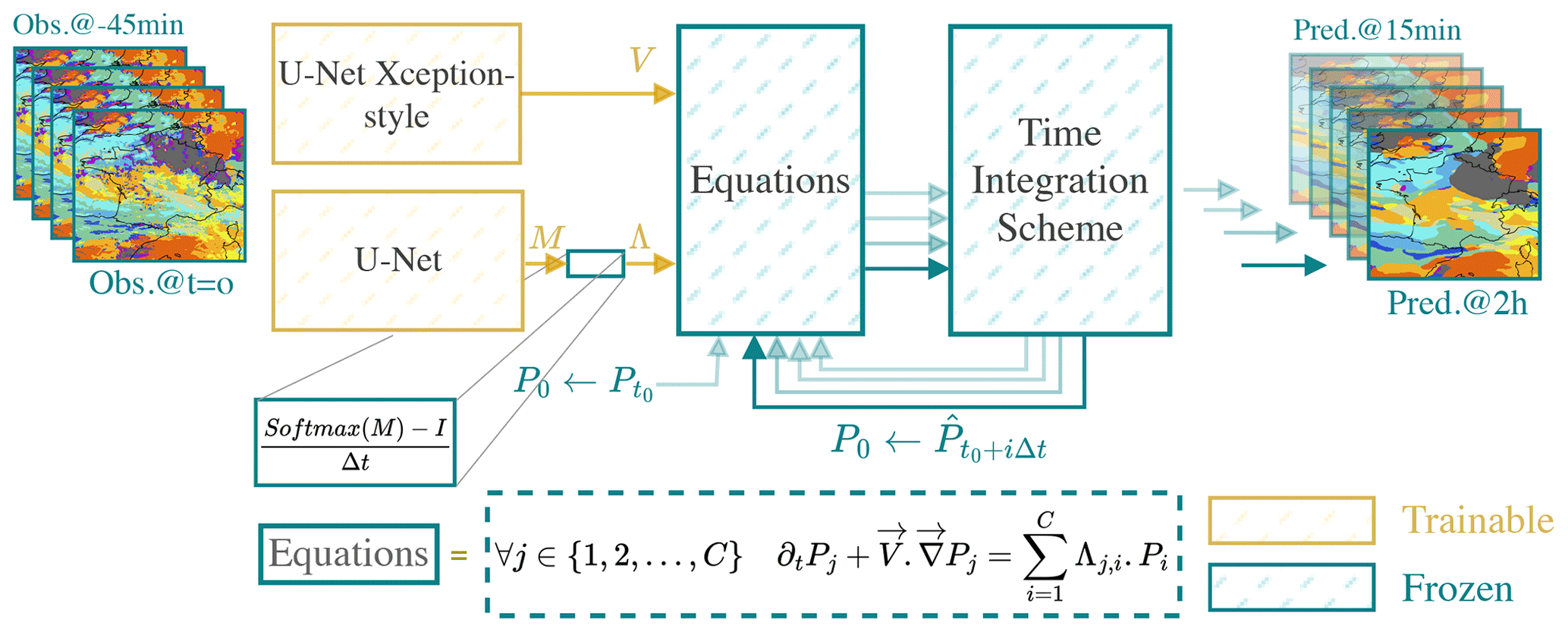
Figure A1 HyPhAICC-3. The third version of the proposed hybrid model. It consists of a U-Net Xception-style model to estimate the velocity field and a second U-Net model to estimate the per-pixel transition matrices from the last observations.

The third version of the hybrid model (see Fig. A1), denoted as HyPhAICC-3, uses this source term combined with the advection as shown in the following equations:

$$\begin{array}{}\text{(A1)}& {\partial }_t{P}_j+\mathit{V}\cdot \mathbf{\nabla }{P}_j=\sum _{i=\mathrm{1}}^C{\mathbf{\Lambda }}_{j,i}{P}_i\forall j\in \left\{\mathrm{1},\mathrm{2},\mathrm{\dots },C\right\},\end{array}$$

where the stochastic property of Π is ensured by construction using the Softmax function as follows:

$${\mathrm{\Pi }}_{i,k}=\text{Softmax}{\left(M_i\right)}_k={\displaystyle \frac{e^{M_{i,k}}}{{\sum }_{j=\mathrm{1}}^C{e}^{M_{i,j}}}},$$

where the matrix M is generated using a U-Net model.

This representation of cloud cover dynamics offers a comprehensive description of cloud formation and dissipation. However, it increases the output dimension size of U-Net, as a C×C transition matrix is generated for each pixel. This makes the U-Net model poorly constrained. Furthermore, in our experiments, we noticed an increased memory usage during the training.

A2 Advection with source term: HyPhAICC-4

To reduce the number of values output by U-Net, we assume a limited number of transition regimes, each representing one of the most frequent transitions. For instance, in the case of two regimes, the source term is described as follows:

$${\partial }_t{P}_j={\mathit{\alpha }}^{\mathrm{1}}\cdot \sum _{i=\mathrm{1}}^C{\mathrm{\Lambda }}_{j,i}^{\mathrm{1}}{P}^i+{\mathit{\alpha }}^{\mathrm{2}}\cdot \sum _{i=\mathrm{1}}^C{\mathrm{\Lambda }}_{j,i}^{\mathrm{2}}{P}^i,$$

where Λ¹ and Λ² are the transition matrices and α¹ and α² are positive factors. These factors determine which regime to consider at each pixel, with the constraint that ${\mathit{\alpha }}^{\mathrm{1}}+{\mathit{\alpha }}^{\mathrm{2}}\le \mathrm{1}$.

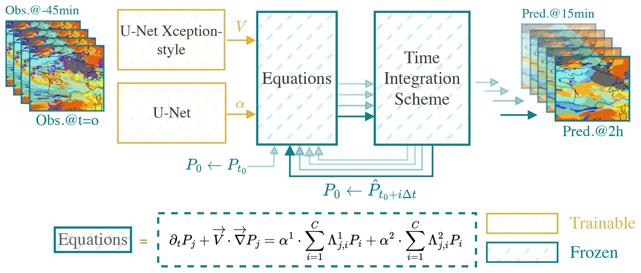
Figure A2 HyPhAICC-4. The fourth version of the proposed hybrid model. It consists of a U-Net Xception-style model to estimate the velocity field and a second U-Net model to estimate the α factors from the last observations. These factors are used to choose which transition regime to consider for each pixel.

The fourth version of the hybrid model, denoted as HyPhAICC-4, uses this source term in addition to the advection as described in the following equations:

$$\begin{array}{}\text{(A2)}& {\partial }_t{P}_j+\mathit{V}\cdot \mathbf{\nabla }{\mathit{P}}_{\mathit{j}}={\mathit{\alpha }}^{\mathrm{1}}\cdot \sum _{i=\mathrm{1}}^C{\mathrm{\Lambda }}_{j,i}^{\mathrm{1}}{P}^i+{\mathit{\alpha }}^{\mathrm{2}}\cdot \sum _{i=\mathrm{1}}^C{\mathrm{\Lambda }}_{j,i}^{\mathrm{2}}{P}^i,\end{array}$$

where α¹ and α² are estimated using U-Net and Λ¹ and Λ² are learned as model parameters (see Fig. A2).

HyPhAICC-3 and HyPhAICC-3 are trained using the same dataset and training procedure as for HyPhAICC-1 and HyPhAICC-2. However, during training the Λ matrices in Eqs. (A1) and (A2) are consistently estimated as zeros. In other words, no inter-class transitions were captured.

A3 Scores

Figure A3 represents the score comparison shown in Fig. 6 but with additional confidence intervals. These confidence intervals were estimated using bootstrapping with a threshold of 99 %.

A4 Full-disc predictions

Figure A4 shows predictions of the HyPhAICC-1 model on the Earth's full disc centred at 0° longitude.

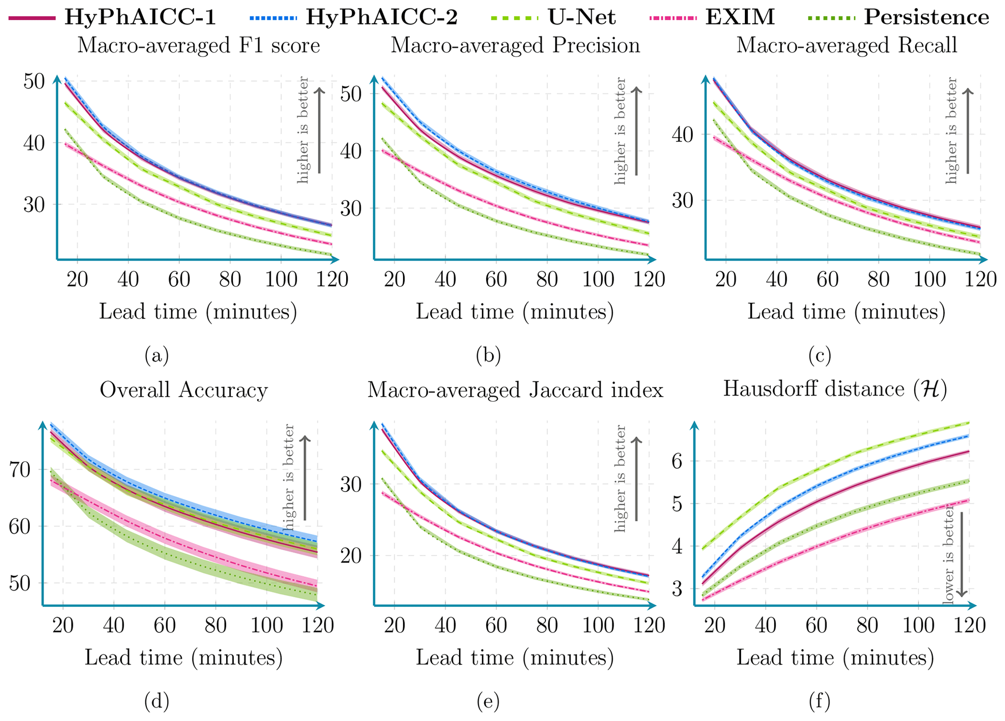
Figure A3 Performance comparison between HyPhAICC-1, U-Net, EXIM, and the persistence baseline using five metrics, including averaged F1 score (%), precision (%), recall (%), accuracy (%), CSI (%), and Hausdorff distance (defined in Eq. 9). These scores were computed over 1000 random samples covering France in 2021. The confidence intervals were estimated using bootstrapping with a threshold of 99 %.

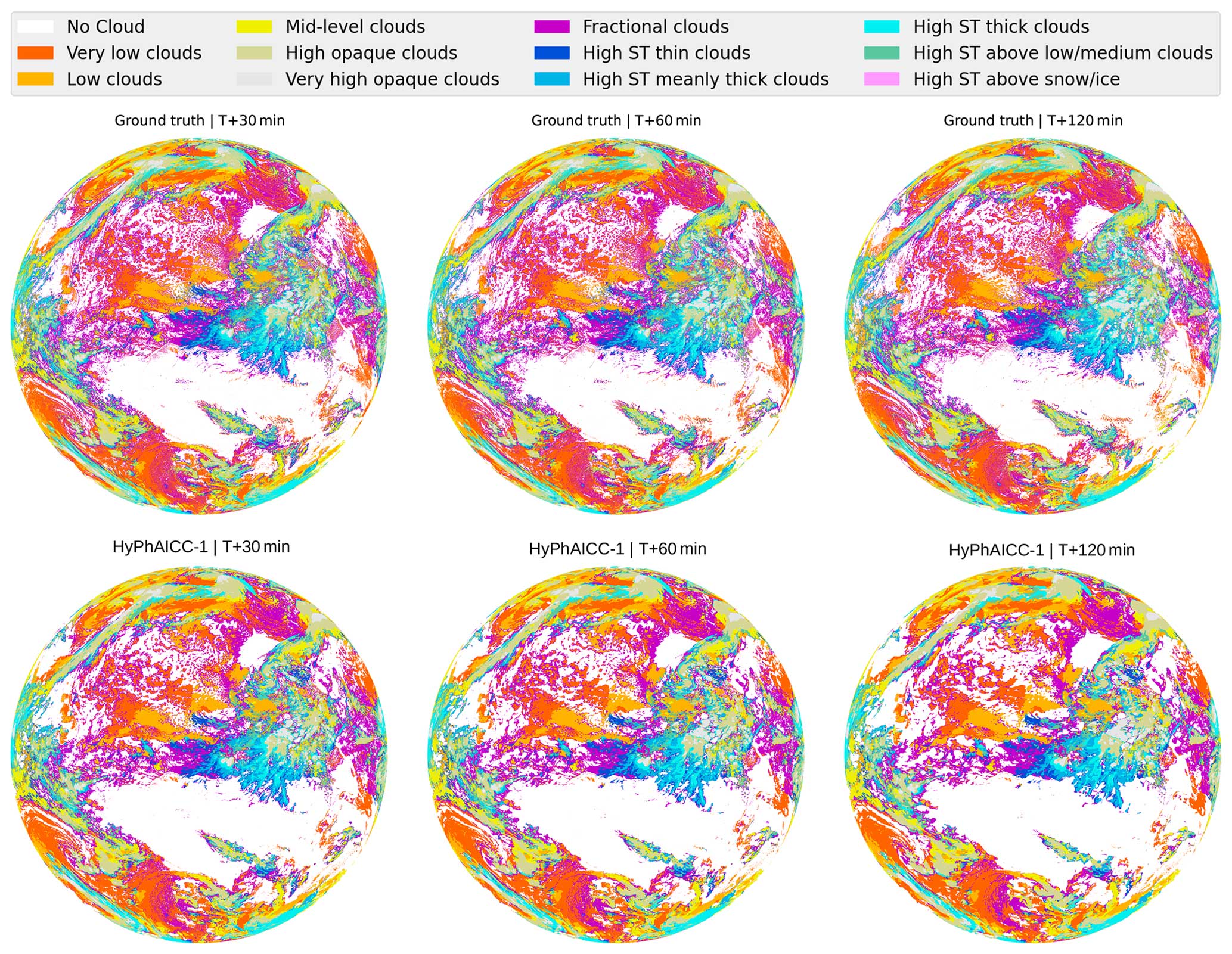
Figure A4 Full-disc cloud cover nowcasting predictions. The predictions were generated by our model without any specific training on the full disc data (of size 3712×3712).

Appendix B: Bridging neural networks and numerical modelling

In this section, we present fundamental components for implementing the proposed hybrid architecture. In Sect. B1 we explore the integration of physics within a neural network. We then explain the trainability challenges associated with this architecture in Sect. B2. Following this, in Sect. B3 we provide a brief introduction to numerical methods for solving PDEs. Finally, in Sect. B4 and B5, we present the method used to approximate derivatives and perform time integration within a neural network.

B1 Combining neural networks and physics

An artificial neural network is a function f_θ parameterised by a set of parameters θ. It results from the composition of a sequence of elementary non-linear parameterised functions called layers that process and transform input data x into output predictions y as follows:

$$\begin{array}{}\text{(B1)}& y=f_{\mathit{\theta }}\left(x\right).\end{array}$$

Physics-based models aim to represent the underlying physical processes or equations that govern the behaviour of a system. To incorporate physics into the neural network, one possible approach involves feeding the output of the physics-based model as an input to the neural network as follows:

$$\begin{array}{}\text{(B2)}& y=f_{\mathit{\theta }}\left(x,\mathit{\varphi }\left(x_{\text{Phy}}\right)\right),\end{array}$$

where x_Phy are the inputs of the physics-based model ϕ. This method could be effective when the physics-based model is self-contained and its components are explicitly known. However, it becomes impractical in scenarios where the physics-based model presents unknown variables that need to be estimated. This is the case in the application considered in this work, where the cloud motion field is unknown. In such instances, a more suitable approach is to pursue a joint resolution. Here, the physical model takes the outputs of the neural network and computes the predictions, resulting in a composition of f_θ and ϕ as follows:

$$\begin{array}{}\text{(B3)}& y=\mathit{\varphi }\circ f_{\mathit{\theta }}\left(x,x_{\text{Phy}}\right).\end{array}$$

In this approach, ϕ implicitly applies a hard constraint on these outputs. This might contribute to accelerate the convergence of the neural network during the training process.

Unlike the first method (Eq. B2), where the physics-based model ϕ is passive and not involved in the training procedure, the second method raises some challenges concerning the trainability of the architecture.

B2 Training a neural network

Neural networks learn to minimise a loss function ℒ_θ by adjusting its set of parameters θ using data. The loss function measures the error between the predicted outcomes $\widehat{y}$ and the ground truth y. It is expressed as

$$\begin{array}{}\text{(B4)}& {\mathcal{L}}_{\mathit{\theta }}={\displaystyle \frac{\mathrm{1}}{N}}\sum _{k=\mathrm{1}}^{N}l(y_k,f_{\mathit{\theta }}\left(x_k\right)),\end{array}$$

where N is the sample size and l is a measure of the discrepancy between the ground truth y_i and the model's production associated with the input x_i, i.e. f_θ∘ϕ(x_i). For instance, using $l(a,b)=\parallel a-b{\parallel }^{\mathrm{2}}$ is the measure used to calibrate a regression model, and ℒ_θ is then the so-called mean-squared error (MSE).

During this training process, an algorithm called backpropagation is used to optimise model parameters. Backpropagation involves computing the gradient of the loss function with respect to the network's parameters. It indicates how much each weight contributed to the error. This gradient is then used to update the parameters in the direction that minimises ℒ_θ, following a sequential optimisation algorithm such as gradient descent, as described below:

$$\begin{array}{}\text{(B5)}& {\mathit{\theta }}_{\text{updated}}={\mathit{\theta }}_{\text{old}}-\mathit{\gamma }\mathrm{\nabla }{\mathcal{L}}_{{\mathit{\theta }}_{\text{old}}},\end{array}$$

where γ is the magnitude of the descent. In order to perform the backpropagation, we assume that the gradient of the loss function with respect to the model's parameters could be calculated using the chain rule. This assumption is called differentiability. Indeed, neural networks rely on activation functions and operations that are differentiable, allowing the gradients to be propagated backward through the network layers.

In this proposed hybrid approach, PDEs are solved to produce model predictions. If the PDE solver includes non-differentiable steps, the chain rule breaks down, making it impossible to compute gradients within the standard deep-learning frameworks. In what follows, we describe our strategy for modelling and solving PDEs using basic differentiable operations commonly employed in neural networks.

B3 Numerical methods for partial differential equations

Numerical weather prediction involves addressing equations of the form

$$\begin{array}{}\text{(B6)}& {\partial }_{t}f=\mathcal{F}\left(f,{\partial }_{x}f,{\partial }_x^{\mathrm{2}}f,\mathrm{\dots }\right),\end{array}$$

governing the evolution of a univariate or multivariate field f over time. Computers cannot directly solve symbolic PDEs, and a common approach involves a two-stage process to transform the PDE into a mathematical formulation more suitable for computational handling. This process begins by discretising the partial derivatives with respect to spatial coordinates, resulting in an ordinary differential equation. Subsequently, a temporal integration describes the evolution of the system over time.

Spatial discretisation can be performed using several methods, e.g. finite volumes, finite elements, or spectral methods. However, the simplest one, the finite-difference method, consists of replacing spatial derivatives of f with quantities that depend on the values of f on a grid. For example, on a 1D periodic domain [0,L] of coordinate x, discretised in N grid points ${\left(x_i\right)}_{[\mathrm{0},n-\mathrm{1}]}$ (x_n=x₀), the central difference method of the first-order spatial derivative reads

$$\begin{array}{}\text{(B7)}& {\partial }_{x}f(t,x_i)\approx {\displaystyle \frac{f(t,x_{i+\mathrm{1}})-f(t,x_{i-\mathrm{1}})}{\mathrm{2}\mathit{\delta }x}},\end{array}$$

where $\mathit{\delta }x=x_{i+\mathrm{1}}-x_i$ represents the grid resolution. Following spatial discretisation, Eq. (B6) can be written as an ordinary differential equation as follows:

$$\begin{array}{}\text{(B8)}& {\displaystyle \frac{\mathrm{d}\mathbf{\text{f}}}{\mathrm{d}t}}=\widehat{F}\left(\mathbf{\text{f}}\right),\end{array}$$

where f(t) is the discretised form of f over the spatial domain, i.e. the vector of grid-point values of f at time t, giving $\mathbf{\text{f}}\left(t\right)=\left(f\right(t,x_i){)}_i$ in the 1D domain mentioned above.

For the time integration, various methods can also be employed, e.g. Euler's method or a fourth-order Runge–Kutta method (RK4) (Runge, 1895; Kutta, 1901). These methods differ in their accuracy, stability, and computational cost. An explicit Euler time integration of Eq. (B8) reads

$$\begin{array}{}\text{(B9)}& {\mathbf{\text{f}}}_{q+\mathrm{1}}={\mathbf{\text{f}}}_q+\mathit{\delta }t\widehat{F}\left({\mathbf{\text{f}}}_q\right),\end{array}$$

where f_q=f(t_q) and t_q=qδt is the discretised time of time step δt.

For the sake of illustration, we consider the advection over the above-mentioned 1D periodic domain, given by the following equation:

$$\begin{array}{}\text{(B10)}& {\partial }_{t}f+u{\partial }_{x}f=\mathrm{0},\end{array}$$

where u is a velocity field, whose values on the grid are denoted as $(u_i{)}_{i\in [\mathrm{0},n-\mathrm{1}]}$. Applying central difference and an Euler scheme discretisation yields the following sequential evolution:

$$\begin{array}{}\text{(B11)}& f_{q+\mathrm{1},i}=f_{q,i}-{\displaystyle \frac{\mathit{\delta }t}{\mathrm{2}\mathit{\delta }x}}{u}_i\left(f_{i+\mathrm{1}}-f_{i-\mathrm{1}}\right).\end{array}$$

This example illustrates the integration of the advection equation over time using a simple explicit method. However, depending on the problem characteristics and requirements, other time integration schemes may be more suitable.

In this study, we propose to model and solve PDEs within a neural network, e.g. equations of the form Eq. (B6). This is achieved by describing the equivalent of spatial and temporal discretisation in the frame of neural network layers, i.e. how it can be implemented in a deep-learning (DL) framework as TensorFlow (Abadi et al., 2016) or PyTorch (Paszke et al., 2019).

B4 Finite-difference methods and convolutional layers

To implement a finite-difference discretisation, one viable approach is to employ the convolution operation. For instance, the 1D convolution associated with Eq. (B7) can be mathematically written as follows:

$$\begin{array}{}\text{(B12)}& (K^{\mathrm{1}}\cdot f)\left[i\right]=\sum _{m=\mathrm{0}}^{M-\mathrm{1}}{K}^{\mathrm{1}}\left[i\right]f\left[m+i\right],\end{array}$$

where K¹ is the kernel or filter used for the convolution and expressed as

$$K^{\mathrm{1}}=\left[\begin{array}{ccc}\frac{-\mathrm{1}}{\mathrm{2}\mathit{\delta }x}& \mathrm{0}& \frac{\mathrm{1}}{\mathrm{2}\mathit{\delta }x}\end{array}\right],$$

and f represents the input data. The variable M corresponds to the size of the kernel. It is the number of finite-difference coefficients, also called stencil size. In this case, a three-point stencil is considered (M=3). Finally, ∗ is the convolution operator.

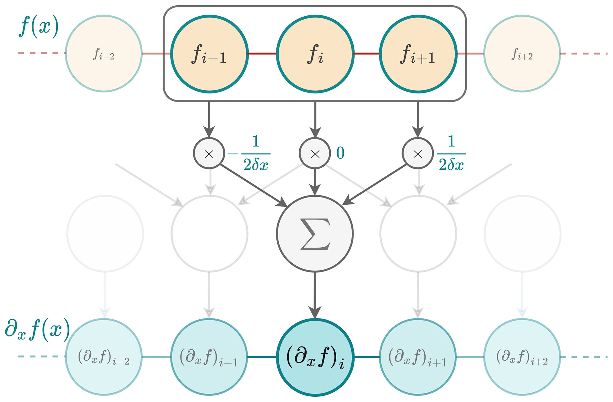
Figure B1 In order to calculate the numerical derivative of f, a kernel K¹ is used to slide across an input vector, which is a discretised version of f with N elements, multiplying values element-wise within its window and summing the results to approximate the derivative at each position. The result is a new vector of size N−2 containing the numerical derivative of f (padding at the bounds with zeros or duplicated values in the input vector can be applied to produce an output vector of size N). This is equivalent to a convolution between K¹ and f and can be reproduced using a 1D convolutional layer with K¹ as a kernel.

This leads to an interesting interaction with DL frameworks. Indeed, convolutional neural networks (CNNs) rely on the operation

$$\text{ConvLayer}\left(f\right)\left[i\right]=\mathit{\sigma }\left(\sum _{m=\mathrm{0}}^{M-\mathrm{1}}K\left[m\right]f\left[m+i\right]+b\right),$$

where σ is called activation function and b is a parameter representing the bias. Observing that using data where sigma is equal to identity and b is equal to 0 leads to the same operation as in Eq. (B12), one can leverage deep-learning frameworks to approximate derivatives, which enables derivative-based operations in neural networks, as shown in Fig. B1. The same principle applies to higher derivative orders. For any positive integer α, we can write the approximation of the αth derivative of f as

$$\begin{array}{}\text{(B13)}& {\partial }^{\mathit{\alpha }}f\approx K^{\mathit{\alpha }}\ast f,\end{array}$$

where K^α are the finite-difference coefficients for the αth derivative.

Finally, using convolutions is a straightforward method to model the spatial term of a PDE, also called the trend, as follows

$$\begin{array}{}\text{(B14)}& \widehat{F}\left(f\right)=\mathcal{N}\left(f\right).\end{array}$$

This results in a neural network that can be used for time integration.

Figure B2 Illustration of a residual block.

B5 Temporal schemes and residual networks

The time integration expressed in Eq. (B9) can be written using the neural network implementation 𝒩 of the trend as

$$\begin{array}{}\text{(B15)}& f_{n+\mathrm{1}}=f_n+\mathrm{\Delta }t\mathcal{N}\left(f_n\right).\end{array}$$

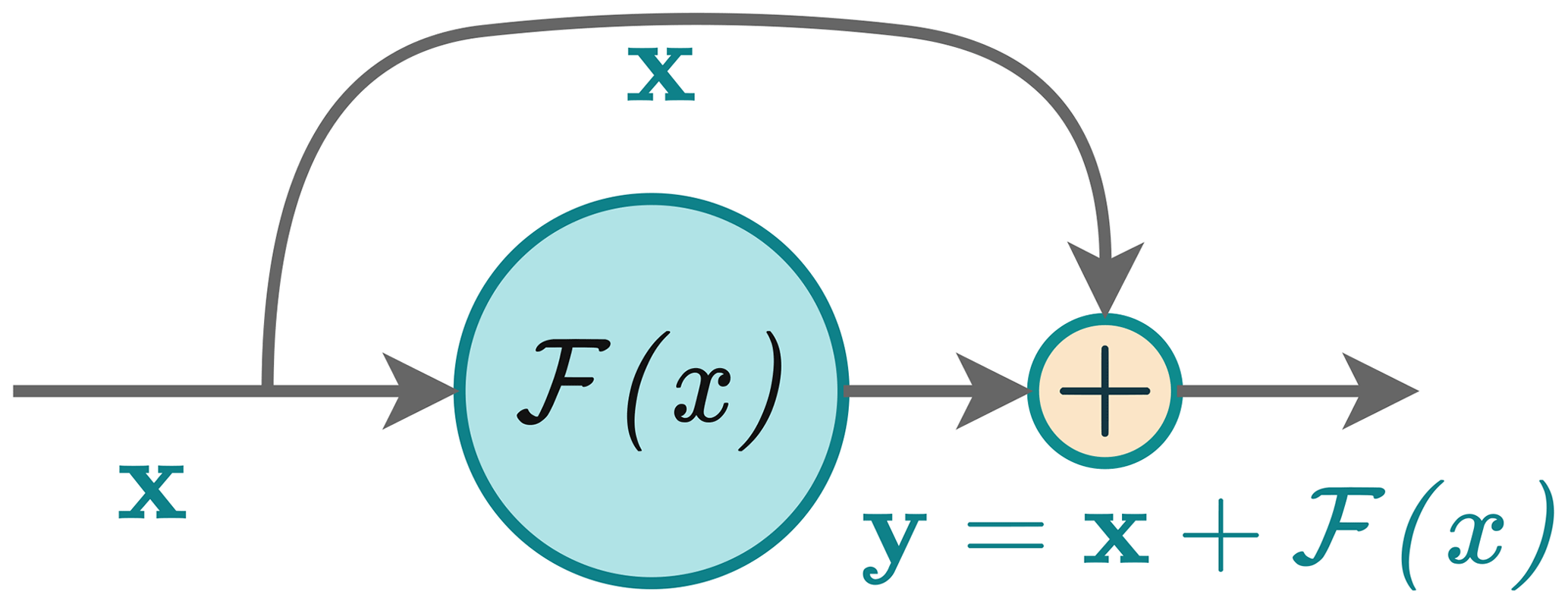
Interestingly, this formulation is very similar to that of a building block commonly used in deep neural networks called a residual block (see Fig. B2), proposed in the ResNet architecture (He et al., 2016). It is formulated as follows:

$$\begin{array}{}\text{(B16)}& y=x+\mathcal{F}\left(x\right),\end{array}$$

where x is the input to the block, y is the output, and ℱ is called a residual function and is made up of multiple neural layers. These layers represent the difference between the input and output. This function aims to capture the additional information or adjustments needed to transform the input into the desired output. This similarity between residual blocks and time schemes, also observed in Ruthotto and Haber (2020), Chen et al. (2018), and Fablet et al. (2017), suggests that the time integration step can be done inside a neural network. All we need is the residual function, which can be modelled using convolutional layers, as shown previously. Pannekoucke and Fablet (2020) proposed a general framework (called PDE-NetGen (https://github.com/opannekoucke/pdenetgen, last access: 7 June 2024) to model a PDE in a neural network form using this method. Residual blocks were originally designed to address vanishing gradient issues in image classification tasks. Intriguingly, these blocks proved to function similarly to time schemes, where they introduce small changes over incremental time steps. This challenges the traditional black box perception of neural networks, although full interpretability remains a distant goal.

Appendix C: Robustness of hybrid formulation to changes in coordinates

In a given coordinate system x=(x_i), the advection of a passive scalar c(t,x) by a velocity field u=(u_i) reads as follows:

$$\begin{array}{}\text{(C1)}& {\partial }_{t}c+u_i{\partial }_{x_i}c=\mathrm{0}.\end{array}$$

A change in coordinate system from the coordinate system x to the coordinate system y=(y_j) related by x=x(y) changes this to the following equation:

$$\begin{array}{}\text{(C2)}& {\partial }_{t}C+v_j{\partial }_{y_j}C=\mathrm{0},\end{array}$$

where $C(t,y)=c(t,x(y\left)\right)$ and the velocity v=(v_j) is deduced from the chain rule

$$\begin{array}{}\text{(C3)}& v_j=u_i{\partial }_{x_i}{y}_j,\end{array}$$

(using Einstein's summation convention).

Since HyPhAICC architecture estimates a velocity field from the data that is either u or v depending on the choice of the coordinate system, it implicitly accounts for the chain rule Eq. (C3). As a result, the HyPhAICC architecture is not sensitive to the coordinate system and can apply to regional domain and global projections. However, numerical effects due to the finite spatio-temporal resolution associated with the discretisation can lead to abnormal distortion of signals after several time steps of integration; e.g. the disc resulting from an orthographic projection of the Earth may be deformed by the advection near its boundaries unless the velocity field is close to zero, meaning that the apparent displacement is small.

Note that this relative invariance of HyPhAICC to the choice of coordinate is because it only concerns the advection of a scalar field. Covariant transport of vector or tensor fields would imply additional terms (Christoffel symbols, e.g. Nakahara, 2003) that would break the invariance of HyPhAICC as it is formulated here.

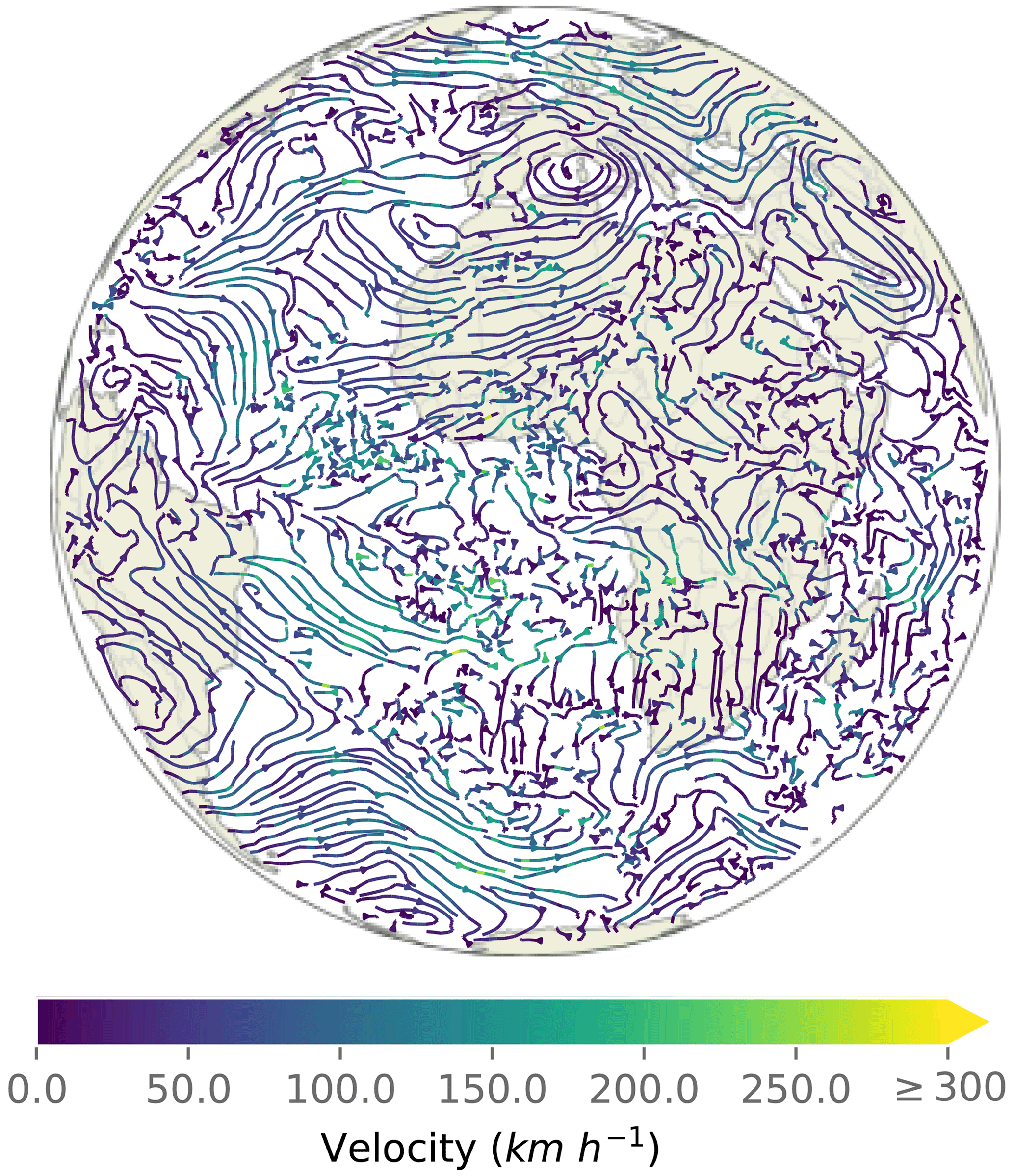
Figure C1 Estimated velocity field from the U-Net Xception-style architecture used in the HyPhAICC-1 model.

Appendix D: Probability advection

Here, we are considering a three-class problem where we have a discrete random variable X with values in the set $\mathrm{1},\mathrm{2},\mathrm{3}$, and we denote X(t,x) using the value of X at time t and space x, with $t\in \left[\mathrm{0},T\right]$ and $x\in \left[\mathrm{0},L\right]$. We are interested in studying the evolution of the state probabilities of X with respect to t and x. For this purpose, we define a vector 𝒫 as

$$\mathcal{P}=\left[\begin{array}{c}{P}_X^{\mathrm{1}}\\ P_X^{\mathrm{2}}\\ P_X^{\mathrm{3}}\end{array}\right].$$

Here, $P_X^c(t,x)$ represents the probability of the c^th class:

$$P_X^c(t,x)=P\left(X\right(t,x)=c).$$

For the sake of simplicity, a 1D problem is considered, but the same analysis applies to the 2D case and for N-class problems with N≥2. Let us consider the following partial differential equation governing the evolution of 𝒫(x,t):

$$\begin{array}{}\text{(D1)}& {\partial }_t\mathcal{P}(x,t)+\mathcal{L}\left(\mathcal{P}(x,t)\right)=\mathrm{0},\end{array}$$

where ℒ is a differential operator. This equation can be written component-wise as follows:

$$\begin{array}{}\text{(D2)}& \left\{\begin{array}{c}{\partial }_t{P}_X^{\mathrm{1}}(x,t)+\mathcal{L}\left(P_X^{\mathrm{1}}(x,t)\right)=\mathrm{0}\\ {\partial }_t{P}_X^{\mathrm{2}}(x,t)+\mathcal{L}\left(P_X^{\mathrm{2}}(x,t)\right)=\mathrm{0}\\ {\partial }_t{P}_X^{\mathrm{3}}(x,t)+\mathcal{L}\left(P_X^{\mathrm{3}}(x,t)\right)=\mathrm{0}\end{array}\right..\end{array}$$

As already discussed in Sect. 2.2.1, three properties should be checked in order to ensure the probabilistic nature of P.

1. Non-negativity. $P(\mathbf{x},t)\ge \mathrm{0}$ for all values of x and t, with $\mathbf{x}=(x,y)$, which ensures that the probabilities remain non-negative.

2. Bound preservation. $P(\mathbf{x},t)\le \mathrm{1}$ for all values of x and t, which ensures that no probability exceeds 1.

3. Probability conservation. ${\sum }_{i=\mathrm{1}}^C{P}_X^i(\mathbf{x},t)=\mathrm{1}$ for all values of x and t, with C=12 being the total number of cloud types. This property guarantees that the sum of all probabilities is equal to 1.

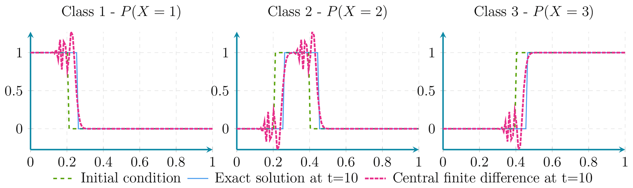
Figure D1 Here it can be seen that the advection of probabilities using central finite-difference discretisation presents a dispersion effect.

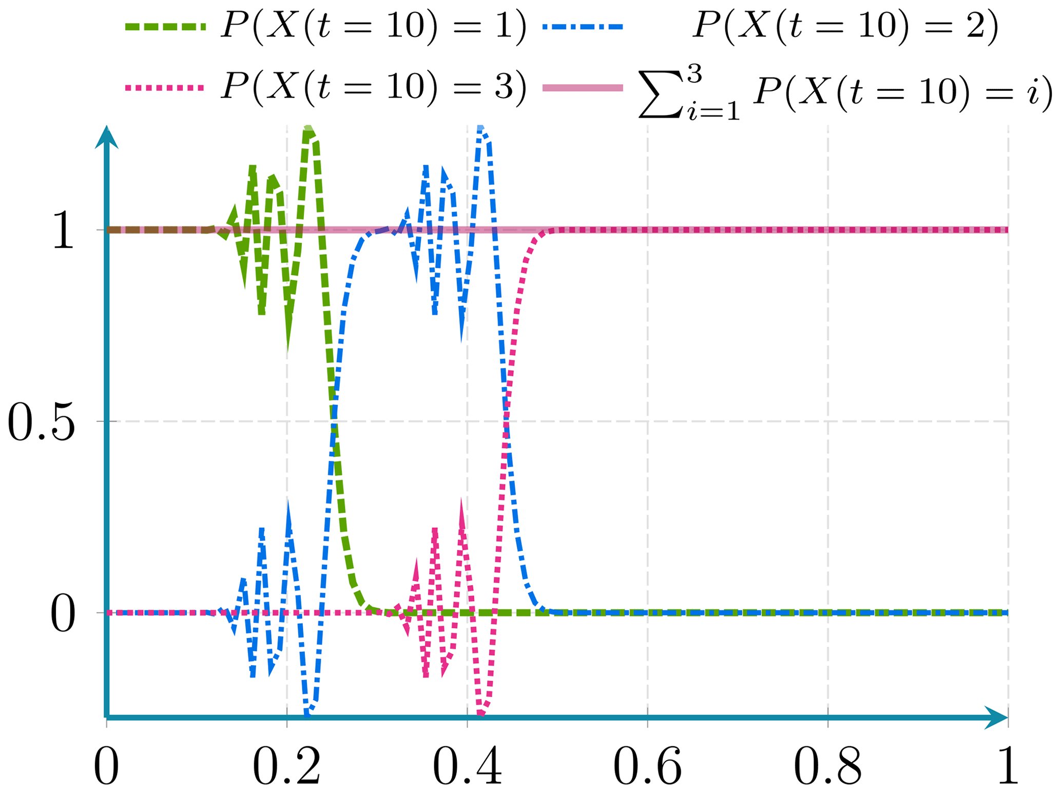
Figure D2 Here the probability conservation property is maintained even in presence of dispersion effects.

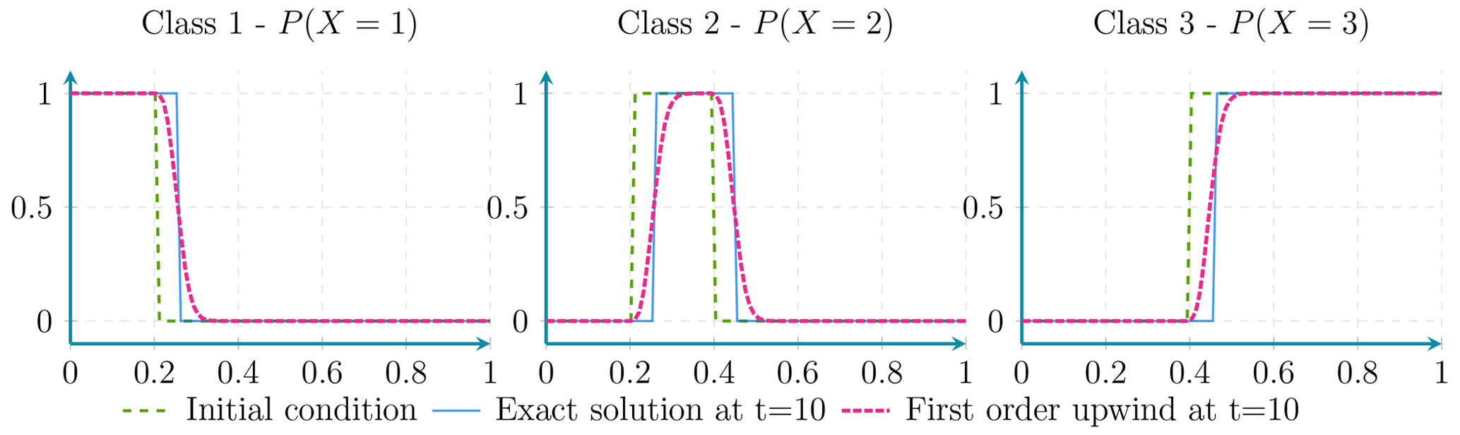
Figure D3 Here the advection of probabilities using first-order upwind discretisation presents a diffusion effect.

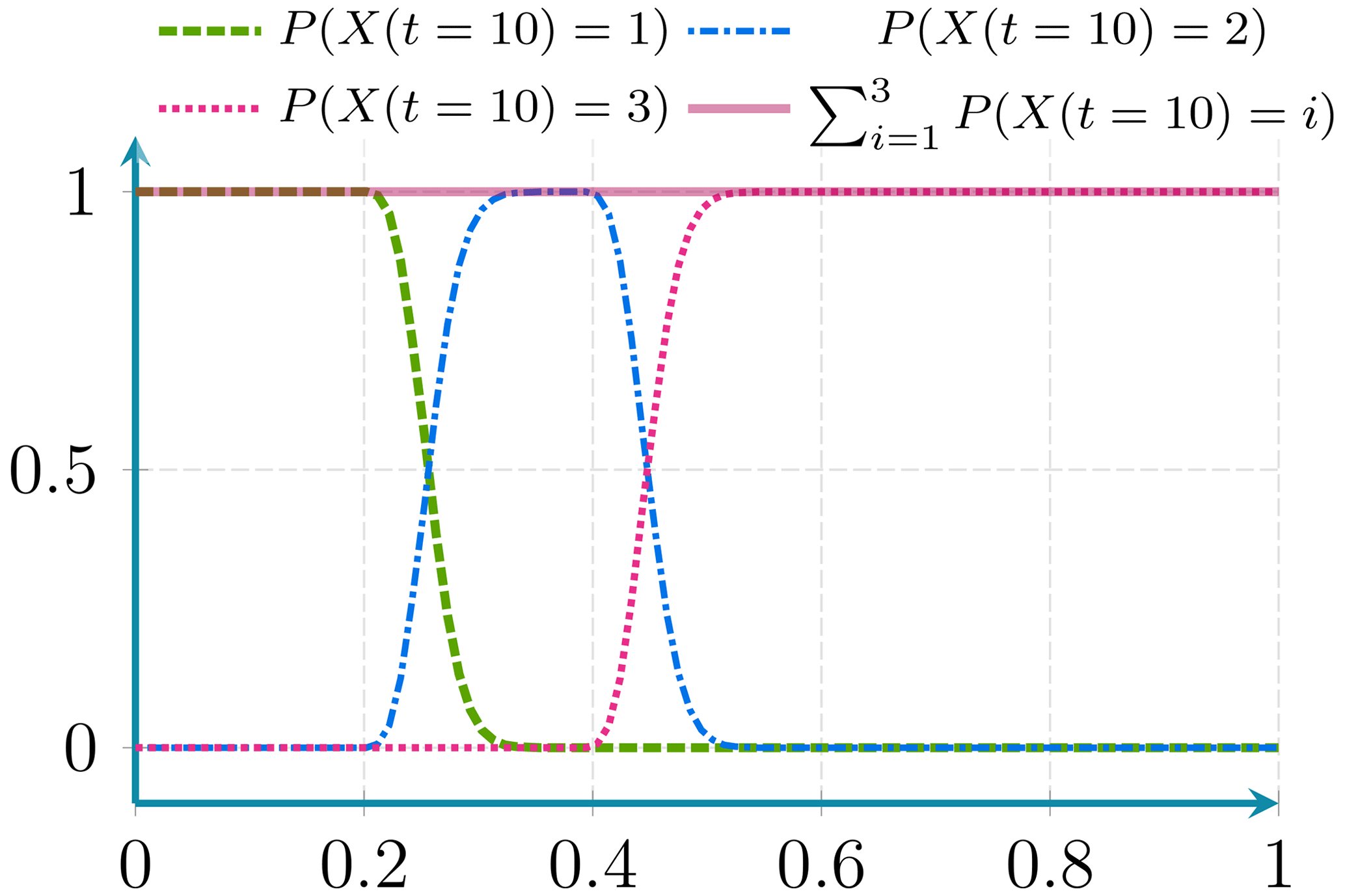
Figure D4 Here the probability conservation property is maintained even in presence of diffusion effects.

D1 Probability conservation

Property. The probability conservation property is ensured if ℒ is a linear differential operator with non-zero positive spatial derivative orders.

Proof. Let us sum the three equations in Eq. (D2) for the specific case where ℒ is a linear differential operator with non-zero positive spatial derivative orders.

$$\begin{array}{rl}& \sum _{i=\mathrm{1}}^{\mathrm{3}}{\partial }_t{P}_X^i(x,t)+\mathcal{L}\left(P_X^i(x,t)\right)=\mathrm{0}\\ & {\partial }_t\sum _{i=\mathrm{1}}^{\mathrm{3}}{P}_X^i(x,t)=-\sum _i^{\mathrm{3}}\mathcal{L}\left(P_X^i(x,t)\right).\end{array}$$

Assuming ${\sum }_{i=\mathrm{1}}^{\mathrm{3}}{P}_X^i(x,t_{\mathrm{0}})=\mathrm{1}$, the linearity property of ℒ allows us to interchange the summation and the operator, resulting in the following equation:

$$\begin{array}{ll}{\displaystyle }\sum _i^{\mathrm{3}}\mathcal{L}\left(P_X^i(x,t_{\mathrm{0}})\right)& {\displaystyle }=-\mathcal{L}\left(\sum _{i=\mathrm{1}}^{\mathrm{3}}{P}_X^i(x,t_{\mathrm{0}})\right)\\ {\displaystyle }& {\displaystyle }=-\mathcal{L}\left(\mathrm{1}\right)\\ {\displaystyle }& {\displaystyle }=\mathrm{0}.\end{array}$$

ℒ(1)=0 as ℒ only has derivatives with positive non-zero orders.

Applying and summing the first-order Taylor expansion at t₀ on each of the time derivatives of Eq. (D2) gives

$$\begin{array}{ll}{\displaystyle }\sum _i^{\mathrm{3}}{\displaystyle \frac{P_i(x,t_{\mathrm{0}}+\mathit{\delta }t)-P_i(x,t_{\mathrm{0}})}{\mathit{\delta }t}}+\mathcal{O}\left(\mathrm{1}\right)& {\displaystyle }=-\sum _i^{\mathrm{3}}\mathcal{L}\left(P_X^i(x,t)\right)\\ {\displaystyle }& {\displaystyle }=\mathrm{0}\end{array}$$

$$\sum _i^{\mathrm{3}}{P}_i(x,t_{\mathrm{0}}+\mathit{\delta }t)=\sum _i^{\mathrm{3}}{P}_i(x,t_{\mathrm{0}})+\mathcal{O}\left(\mathit{\delta }t\right),$$

when δt is small enough, ${\sum }_i^{\mathrm{3}}{P}_i(x,t_{\mathrm{0}}+\mathit{\delta }t)=\mathrm{1}$.

Iteratively, starting from t₀, ∀t

$$\sum _i^{\mathrm{3}}{P}_i(x,t)=\sum _i^{\mathrm{3}}{P}_i(x,t_{\mathrm{0}})=\mathrm{1}.$$

In this study, we consider the advection equation using the same velocity field for all probability maps, where the operator ℒ is written as follows:

$$\mathcal{L}\left(P_i\right)=u\cdot {\partial }_x{P}_i,i\in \mathit{\{}\mathrm{1},\mathrm{2},\cdot ,\mathrm{12}\mathit{\}}.$$

This differential operator is linear and has a non-zero positive derivative order. Therefore, the sum of probabilities is conserved over time and remains equal to the initial value. This property is illustrated numerically in Figs. D2 and D4, and it is maintained independently of the discretisation scheme.

D2 Non-negativity and bound preservation

In order to check the two other properties, we need to study the discretisation schemes.

Out of the four numerical schemes studied (central finite differences, semi-Lagrangian, and first- and second-order upwind), only the semi-Lagrangian and the first-order upwind discretisation satisfy the first and second properties. The remaining two schemes exhibit some form of dispersion.

Details about central finite difference and first-order upwind scheme are given in Sect. E.

Appendix E: Discretisation schemes

Here, we will derive the equivalent equation of central differences and upwind scheme applied to the following advection equation:

$$\begin{array}{}\text{(E1)}& {\displaystyle \frac{\partial F(x,t)}{\partial t}}+u{\displaystyle \frac{\partial F(x,t)}{\partial x}}=\mathrm{0}.\end{array}$$

E1 Central differences: equivalent equation

We consider the second-order central discretisation in space and a first-order explicit forward difference in time applied to the advection equation.

$$\begin{array}{}\text{(E2)}& {\displaystyle \frac{F_i^{n+\mathrm{1}}-F_i^n}{\mathrm{\Delta }t}}+u_i{\displaystyle \frac{F_{i+\mathrm{1}}-F_{i-\mathrm{1}}}{\mathrm{2}\mathrm{\Delta }x}}=\mathrm{0}\end{array}$$

Using the Taylor formulas in Eq. (E2), we get

$$\begin{array}{}\text{(E3)}& \begin{array}{rl}{\partial }_{t}F& +{\displaystyle \frac{\mathrm{\Delta }t}{\mathrm{2}}}{\partial }_t^{\mathrm{2}}F+\mathcal{O}\left(\mathrm{\Delta }{t}^{\mathrm{2}}\right)\\ & =-u\left({\partial }_{x}F-{\displaystyle \frac{\mathrm{\Delta }{x}^{\mathrm{2}}}{\mathrm{6}}}{\partial }_x^{\mathrm{3}}F+\mathcal{O}\left(\mathrm{\Delta }{x}^{\mathrm{2}}\right)\right)\end{array}.\end{array}$$

However, when we only require a first-order expansion in time, we can replace the second-order time derivative with another term coming from a Taylor first-order expansion of Eq. (E2) :

$$\begin{array}{}\text{(E4)}& {\partial }_t\left({\partial }_{t}F\right)+\mathcal{O}\left(\mathrm{\Delta }t\right)=-{\partial }_t\left(u{\partial }_{x}F\right)+\mathcal{O}\left(\mathrm{\Delta }x\right),\end{array}$$

which leads to

$${\partial }_t^{\mathrm{2}}F=-{\partial }_{t}u{\partial }_{x}F-u{\partial }_{xt}^{\mathrm{2}}F+\mathcal{O}(\mathrm{\Delta }t,\mathrm{\Delta }x).$$

Using the same approach as in Eq. (E4), the derivative ${\partial }_{xt}^{\mathrm{2}}F$ can be computed as follows:

$${\partial }_x\left({\partial }_{t}F\right)=-{\partial }_{x}u{\partial }_{x}F-u{\partial }_x^{\mathrm{2}}F+\mathcal{O}(\mathrm{\Delta }t,\mathrm{\Delta }x).$$

We replace the derivative ${\partial }_{xt}^{\mathrm{2}}F$ in the last equation as follows:

$$\begin{array}{}\text{(E5)}& \begin{array}{rl}{\partial }_t^{\mathrm{2}}F& =-{\partial }_{t}u{\partial }_{x}F-u\left(-{\partial }_{x}u{\partial }_{x}F-u{\partial }_x^{\mathrm{2}}F\right)\\ & +\mathcal{O}(\mathrm{\Delta }t,\mathrm{\Delta }x)\end{array}.\end{array}$$

Finally, we replace the second-order derivative in Eq. (E3) with the expression in Eq. (E5):

$$\begin{array}{ll}{\displaystyle }& {\displaystyle }{\partial }_{t}F+{\displaystyle \frac{\mathrm{\Delta }t}{\mathrm{2}}}\left(-{\partial }_{t}u{\partial }_{x}F-u\left(-{\partial }_{x}u{\partial }_{x}F-u{\partial }_x^{\mathrm{2}}F\right)\right)\\ {\displaystyle }& {\displaystyle }=-u\left({\partial }_{x}F-{\displaystyle \frac{\mathrm{\Delta }{x}^{\mathrm{2}}}{\mathrm{6}}}{\partial }_x^{\mathrm{3}}F\right)+\mathcal{O}\left(\mathrm{\Delta }{t}^{\mathrm{2}},\mathrm{\Delta }{x}^{\mathrm{2}}\right).\end{array}$$

Hence,

$$\begin{array}{}\text{(E6)}& \begin{array}{rl}{\partial }_{t}F+\stackrel{\mathrm{̃}}{u}{\partial }_{x}F& =-{\displaystyle \frac{\mathrm{\Delta }t}{\mathrm{2}}}{u}^{\mathrm{2}}{\partial }_x^{\mathrm{2}}F+{\displaystyle \frac{\mathrm{\Delta }{x}^{\mathrm{2}}}{\mathrm{6}}}u{\partial }_x^{\mathrm{3}}F\\ & +\mathcal{O}\left(\mathrm{\Delta }{t}^{\mathrm{2}},\mathrm{\Delta }{x}^{\mathrm{2}}\right),\end{array}\end{array}$$

where $\stackrel{\mathrm{̃}}{u}=u-\frac{\mathrm{\Delta }t}{\mathrm{2}}{\partial }_{t}u+\frac{\mathrm{\Delta }t}{\mathrm{2}}u{\partial }_{x}u$.

E2 First-order upwind scheme: equivalent equation

Now let us consider the first-order upwind discretisation of the spatial term given by

$$\left\{\begin{array}{ll}\frac{F_i^{n+\mathrm{1}}-F_i^n}{\mathrm{\Delta }t}+u\frac{F_i-F_{i-\mathrm{1}}}{\mathrm{\Delta }x}=\mathrm{0}& \text{ if }u\ge \mathrm{0}\\ \frac{F_i^{n+\mathrm{1}}-F_i^n}{\mathrm{\Delta }t}+u\frac{F_{i+\mathrm{1}}-F_i}{\mathrm{\Delta }x}=\mathrm{0}& \text{ if }u<\mathrm{0}\end{array}\right..$$

These two equations can be written as follows:

$$\begin{array}{}\text{(E7)}& {\displaystyle \frac{F_i^{n+\mathrm{1}}-F_i^n}{\mathrm{\Delta }t}}+\left(u_i^{+}{\displaystyle \frac{F_i-F_{i-\mathrm{1}}}{\mathrm{\Delta }x}}+u_i^{-}{\displaystyle \frac{F_{i+\mathrm{1}}-F_i}{\mathrm{\Delta }x}}\right)=\mathrm{0},\end{array}$$

where $u_i^{+}=max(u_i,\mathrm{0})$ and $u_i^{-}=min(u_i,\mathrm{0})$.

Considering the case of u≥0 of Eq. (E7), using the Taylor formulas, we get:

$$\begin{array}{}\text{(E8)}& \begin{array}{rl}{\partial }_{t}F& +{\displaystyle \frac{\mathrm{\Delta }t}{\mathrm{2}}}{\partial }_t^{\mathrm{2}}F+\mathcal{O}\left(\mathrm{\Delta }{t}^{\mathrm{2}}\right)\\ & =-u\left({\partial }_{x}F-{\displaystyle \frac{\mathrm{\Delta }x}{\mathrm{2}}}{\partial }_x^{\mathrm{2}}F+\mathcal{O}\left(\mathrm{\Delta }{x}^{\mathrm{2}}\right)\right)\end{array}.\end{array}$$

As in the case of the central differences, we replace the second-order derivative ${\partial }_t^{\mathrm{2}}F$ in Eq. (E8) with the expression in Eq. (E5).

$$\begin{array}{ll}{\displaystyle }& {\displaystyle }{\partial }_{t}F+{\displaystyle \frac{\mathrm{\Delta }t}{\mathrm{2}}}\left(-{\partial }_{t}u{\partial }_{x}F-u\left(-{\partial }_{x}u{\partial }_{x}F-u{\partial }_x^{\mathrm{2}}F\right)\right)\\ {\displaystyle }& {\displaystyle }=-u\left({\partial }_{x}F-{\displaystyle \frac{\mathrm{\Delta }x}{\mathrm{2}}}{\partial }_x^{\mathrm{2}}F\right)+\mathcal{O}\left(\mathrm{\Delta }{t}^{\mathrm{2}},\mathrm{\Delta }{x}^{\mathrm{2}}\right)\end{array}$$

Hence,

$$\begin{array}{}\text{(E9)}& {\partial }_{t}F+\stackrel{\mathrm{̃}}{u}{\partial }_{x}F=v_{\mathrm{num}}{\partial }_x^{\mathrm{2}}F+\mathcal{O}\left(\mathrm{\Delta }{t}^{\mathrm{2}},\mathrm{\Delta }{x}^{\mathrm{2}}\right),\end{array}$$

where $\stackrel{\mathrm{̃}}{u}=u-\frac{\mathrm{\Delta }t}{\mathrm{2}}{\partial }_{t}u+\frac{\mathrm{\Delta }t}{\mathrm{2}}u{\partial }_{x}u$ and $v_{num}=\frac{u}{\mathrm{2}}\left(\mathrm{\Delta }x-u\mathrm{\Delta }t\right)$.

The equivalent equation of the second case of Eq. (E7) (case u≤0) is written as follows:

$$\begin{array}{}\text{(E10)}& {\partial }_{t}F+\stackrel{\mathrm{̃}}{u}{\partial }_{x}F=v_{\mathrm{num}}{\partial }_x^{\mathrm{2}}F+\mathcal{O}\left(\mathrm{\Delta }{t}^{\mathrm{2}},\mathrm{\Delta }{x}^{\mathrm{2}}\right),\end{array}$$

where $v_{\mathrm{num}}=\frac{u}{\mathrm{2}}\left(-\mathrm{\Delta }x-u\mathrm{\Delta }t\right)$

From Eqs. (E9) and (E10) we can write the equivalent equation as follows:

$$\begin{array}{}\text{(E11)}& {\partial }_{t}F+\stackrel{\mathrm{̃}}{u}{\partial }_{x}F=v_{\mathrm{num}}{\partial }_x^{\mathrm{2}}F+\mathcal{O}\left(\mathrm{\Delta }{t}^{\mathrm{2}},\mathrm{\Delta }{x}^{\mathrm{2}}\right),\end{array}$$

where $\stackrel{\mathrm{̃}}{u}=u-\frac{\mathrm{\Delta }t}{\mathrm{2}}{\partial }_{t}u+\frac{\mathrm{\Delta }t}{\mathrm{2}}u{\partial }_{x}u$ and $v_{\mathrm{num}}=\frac{u}{\mathrm{2}}\left(\text{sign}\left(u\right)\mathrm{\Delta }x-u\mathrm{\Delta }t\right)$..

E3 Conclusion

It should be noted that the finite central difference scheme exhibits instability due to the presence of negative diffusion in the second term in Eq. (E6). However, when using a temporal scheme of higher order than two, the negative diffusion term in Δt can be eliminated, rendering the scheme stable. Nevertheless, the scheme becomes dispersive due to the third-order spatial derivative term, resulting in oscillations during the propagation of sharp signals, such as a front or Heaviside function.

Alternatively, the first-order upwind scheme offers stability but introduces numerical diffusion, affecting the accuracy of the solution, this diffusion is due to the second-order derivative term in Eq. (E11).

Finally, the choice of numerical scheme depends on the specific requirements of the problem, such as the desired accuracy and stability of the solution. To respect the properties described above, we use the first-order upwind scheme, as it does not introduce oscillations in the solution. The first-order upwind scheme is also easy to implement in a differentiable mode. Despite the limitation on the time step linked to the CFL condition, we consider it to be a more appropriate scheme to integrate probability advection in a neural network.