Modelling the water isotope distribution in the Mediterranean Sea using a high-resolution oceanic model (NEMO-MED12-watiso v1.0): evaluation of model results against in situ observations

Stable water isotopes (δ¹⁸O_w and δD_w) have been successfully implemented for the first time in a high-resolution model of the Mediterranean Sea (NEMO-MED12). In this numerical study, model results are compared with available in situ observations to evaluate the model performance of the present-day distribution of stable water isotopes and their relationship with salinity on a sub-basin scale. There is good agreement between the modelled and observed distributions of δ¹⁸O_w in the surface water. The model successfully simulates the observed east–west gradient of δ¹⁸O_w characterising surface, intermediate, and deep waters. The results also show good agreement between the simulated δD_w and the in situ data. The δD_w shows a strong linear relationship with δ¹⁸O_w (r²=0.98) and salinity (r²=0.94) for the whole Mediterranean Sea. Moreover, the modelled relationships between δ¹⁸O_w and salinity agree well with observations, with a weaker slope in the eastern basin than in the western basin. We investigate the relationship of the isotopic signature of the planktonic foraminifera shells (δ¹⁸O_c) with temperature and the influence of seasonality. Our results suggest a more quantitative use of δ¹⁸O records, combining reconstruction with modelling approaches.

1 Introduction

Because of their conservative behaviour, stable water isotopes (δ¹⁸O_w (Eq. 1) and δD_w (Eq. 2)) provide a unique opportunity to assess hydrological processes and study the hydrological cycle in climate system variability. The isotopic composition of seawater (δ¹⁸O_w) is globally linked to salinity because δ¹⁸O_w and salinity are affected by common physical processes (i.e. freshwater fluxes or precipitation–evaporation balance). However, the variation in δ¹⁸O_w is more complex because the water isotopes are subjected to additional fractionation and transport in the atmosphere (Craig and Gordon, 1965). The driving factors include mainly surface fractionation in relation to atmospheric exchange and oceanic mixing processes but also continental runoff in coastal areas and ice processes (sea ice formation and iceberg runoff) in polar regions. The evaporation process preferentially extracts lighter water molecules, and the remaining evaporated seawater becomes rich in heavier isotopes. In contrast, the input of freshwater rich in lighter isotopes by precipitation or river runoff leads to a decrease in the δ¹⁸O_w and δD_w values of seawater. Thus, the salinity and the isotopic compositions of oceanic waters are acquired at the surface; the sinking of surface waters to intermediate or deeper layers does not change these parameters, which can remain stable over long distances until they mix with waters with different properties.

Although water isotopes are among the most widely used proxies in climate research, there are still gaps in our understanding of the processes that control their marine distribution. General circulation models (GCMs) allow us to better understand the past variability in water isotopes documented in various archives and to investigate the relationship between water isotopes and different climate variables. The heavy stable isotopes of water (i.e. deuterium and oxygen-18) have been incorporated into both atmospheric models (e.g. Joussaume et al., 1984; Jouzel et al., 1987; Hoffmann et al., 1998; Brown et al., 2006; Risi et al., 2010a, b; Werner et al., 2011) and oceanic models (Schmidt, 1998, 1999; Paul et al., 1999; Delaygue et al., 2000, 2001; Wadley et al., 2002; Xu et al., 2012), as well as into coupled ocean–atmosphere models (Schmidt et al., 2007; Tindall et al., 2010; Roche et al., 2004; Roche, 2013; Werner et al., 2016; Cauquoin et al., 2019; Shi et al., 2023). In recent decades, δ¹⁸O_w and δD_w data have become increasingly important in paleoclimate modelling studies and have been incorporated into global climate models. The isotopic signals are explicitly simulated to compare them with observations and to quantify processes affecting reconstructed seawater isotopic compositions (Roche, 2013; Schmidt et al., 2007). Previous reviews of water isotope measurements and modelling studies (Galewsky et al., 2016; Jones and Dee, 2018; Bowen et al., 2019) have highlighted the importance of understanding spatial and temporal isotopic variability for a quantitative interpretation of its relationship with climate change, and they have also shown the potential of δ¹⁸O_w to characterise individual water masses. However, water isotopes have not yet been incorporated into a high-resolution regional ocean model. Here, we present the first results of a high-resolution regional dynamical model (at $\mathrm{1}/\mathrm{12}$° horizontal resolution) developed for the Mediterranean Sea (Beuvier et al., 2012a).

In the Mediterranean region, net freshwater fluxes at the sea surface, i.e., the difference between evaporation and precipitation, comprise the main driving factor of the hydrological cycle (Mariotti et al., 2002), and there is no effect of sea ice formation or melting (i.e. no freshwater inflow from ice sheets during the recent “present situation” period). This condition provides a unique opportunity to better understand the spatial and temporal variations in water isotopes in a semi-enclosed basin, away from the interference of sea ice, which is currently poorly represented in models. The negative balance between net freshwater input and evaporation ($P+R-E<\mathrm{0}$) leads to an anti-estuarine pattern in the Mediterranean thermohaline circulation system, with a surface inflow of less saline Atlantic water (AW) through the Strait of Gibraltar, which is then gradually transformed into saltier water and eventually sinks in the Levantine sub-basin to form Levantine Intermediate Water (LIW), which spreads across the eastern Mediterranean at water depths of between 150 and 700 m until it reaches the Strait of Gibraltar to form the Mediterranean Outflow Water (MOW) (Millot and Taupier-Letage, 2005; Lascaratos et al., 1999). The LIW is one of the main water masses in the Mediterranean Sea (Pinardi and Masetti, 2000), contributing to the formation of the Eastern Mediterranean Deep Water (EMDW) in the Adriatic sub-basin and the Western Mediterranean Deep Water (WMDW) in the Gulf of Lions. The MOW plays an important role in the North Atlantic overturning circulation because the excess salt transported by the water mass contributes to increasing the density of the water masses in the convection zones of the deep water formation (Bigg et al., 2003). In the past, the Mediterranean thermohaline circulation was profoundly altered, notably during sapropel events, when deep-water ventilation was strongly reduced in the eastern basin; these changes are well documented by water isotope observations (Rohling et al., 2015, and references therein). It is also possible that major changes will take place in the future as a result of global warming (e.g. Somot et al., 2006; Adloff et al., 2015; Pagès et al., 2020). Understanding the processes that control the circulation of the Mediterranean Sea is therefore a major challenge for understanding climate variability in the Mediterranean basin (e.g. Soto-Navarro et al., 2020).

Compared to other large ocean basins, the Mediterranean Sea can be considered ideal for improving our understanding of the processes that influence and drive oxygen isotope variations and for further developing the existing modelling approach because (i) the water residence time is relatively short (∼ 100 years; Millot and Taupier-Letage, 2005); (ii) all major forcing mechanisms are present, including air–sea interaction, buoyancy fluxes, and wind forcing, with a well-studied salinity and water isotope structure (e.g. Pierre, 1999); (iii) well-marked δ¹⁸O_w of the surface waters of the eastern Mediterranean basin (value up to 2.2 ‰; Gat et al., 1996) has the potential to trace the process of deep water formation and the thermohaline circulation variability; and (iv) a high-spatial-resolution regional model (NEMO-MED12) is available, which is essential for the simulation of realistic ocean dynamics and which can then be used for past climate simulation with the adapted coupled regional model (Vadsaria et al., 2020). Over the last few decades, considerable progress has been achieved in our understanding of the processes and mechanisms governing the distribution of water isotopes in the Mediterranean Sea, through high-quality sampling and measurements (e.g. Gat et al., 1996; Pierre, 1999; LeGrande and Schmidt, 2006). Nonetheless, no specific modelling focused on water isotopes is currently available for the Mediterranean Sea. This study aims to implement water isotopes as passive tracers in the high-resolution dynamical model NEMO-MED12 to enable a direct evaluation of paleoclimate simulation that will then be performed using this modelling platform. We use isotope fluxes from the atmospheric general circulation model LMDZ-iso (Risi et al., 2010b). Our paper focuses on the simulation of the present-day oceanic distribution of δ¹⁸O_w and δD_w. We compare model results with existing observations to assess the model's ability to capture the main features of water isotope distribution in the Mediterranean Sea, as well as the relationship between salinity as a function of δ¹⁸O_w and δD_w. By combining δ¹⁸O_w and temperature, we can calculate equilibrated calcite δ¹⁸O_c values using paleotemperature equations to compare model results with recent biogenic carbonate data. The results are analysed for the eastern Mediterranean basin (EMed) and western Mediterranean basin (WMed) to investigate the processes leading to the isotopic distribution of δ¹⁸O_w and δD_w in the Mediterranean Sea. Knowledge of the present-day variability in the isotopic composition of Mediterranean waters should help further studies dedicated to Mediterranean paleoceanography.

2 Method

2.1 Circulation and ocean dynamic using the NEMO-MED12 model

The dynamical model is the NEMO (Nucleus for European Modelling of the Ocean) free-surface ocean circulation model (Madec and NEMO-Team, 2008) in a regional high-resolution configuration called NEMO-MED12 (Beuvier et al., 2012b). The NEMO-MED12 grid is an extraction from the global ORCA $\mathrm{1}/\mathrm{12}$° grid. This corresponds to a grid cell size of between 6 and 7.5 km from 46 to 30° N and represents a grid size of 567 × 264 points. The NEMO-MED12 domain covers the entire Mediterranean Sea and includes the west of Gibraltar in the Atlantic Ocean (buffer zone) from 30–47° N in latitude and from 11° W–36° E in longitude, where salinity and temperature (3-D fields) are relaxed to the observed climatology (Beuvier et al., 2012a). Water exchange with the Black Sea is represented as a two-layer flow with net budget estimates from Stanev and Peneva (2002). The dynamical simulation (the circulation fields, i.e. U, V, and W) has been forced with atmospheric fluxes from the high-resolution (50 km) ARPERA dataset (Herrmann and Somot, 2008; Herrmann et al., 2010). NEMO-MED12 is forced by ARPERA daily fields of momentum, evaporation, and heat fluxes over the period 1958–2013. For the surface temperature condition, a relaxation term to sea surface temperature (SST) from ERA-40 is applied for the heat flux (Beuvier et al., 2012b). This term acts as a first-order coupling between the ocean model's SST and the atmospheric heat flux (Barnier et al., 1995), ensuring consistency between these two terms. The value of the relaxation coefficient is spatially constant and is taken to be −40 W m⁻² K⁻¹, following the CLIPPER Project (Beuvier et al., 2012b). It corresponds to a 1.2 d restoring timescale for a surface layer of 1 m thickness (Beuvier et al., 2012a).

Numerous studies on ocean dynamics and biogeochemical cycles in the Mediterranean have been carried out using the NEMO-MED12 model (e.g. Brossier et al., 2011; Beuvier et al., 2012b; Soto-Navarro et al., 2014; Ayache et al., 2015a, b, 2016, 2017, 2023; Palmiéri et al., 2015; Guyennon et al., 2015; Richon et al., 2018, 2019). The NEMO-MED12 model represents the main structures of the Mediterranean thermohaline circulation well, with mechanisms having a realistic timescale compared to observations (Ayache et al., 2015a). However, some features of the simulation still need to be improved: for example, the weak formation of the Adriatic Deep Water (AdDW) as shown using anthropogenic tritium (Ayache et al., 2015a) and chlorofluorocarbon (CFC) simulations (Palmiéri et al., 2015). In the western basin, the WMDW is generally well simulated, but the propagation of the recently ventilated deep water to the south of the basin is underestimated (Ayache et al., 2015a; Palmiéri et al., 2015). All the details of the model and its parameterisations are described separately in Beuvier et al. (2012b, a), Palmiéri et al. (2015), and Ayache et al. (2015a).

2.2 Implementing water isotopes in the NEMO model

δ¹⁸O_w and δD_w were implemented in the regional high-resolution model NEMO-MED12 (release 3.4 and 3.6 of the NEMO model). A detailed description of the source code of the water isotope package, with a user guide, is available in the Supplement (see Sect. S1 in the Supplement). The exact version of the model used to produce the results reported in this paper is archived on Zenodo (https://doi.org/10.5281/zenodo.10453745, Ayache et al., 2024; see the Supplement). Abbreviations used in this paper are presented in Table 1.

Table 1 Abbreviations and units.

The hydrogen and oxygen isotope compositions are reported as isotopic ratio anomalies referenced to the Vienna Standard Mean Ocean Water reference value (VSMOW):

$$\begin{array}{}\text{(1)}& {\displaystyle }{\mathit{\delta }}^{\mathrm{18}}\mathrm{O}=\left({\displaystyle \frac{{}^{\mathrm{18}}R}{{}^{\mathrm{18}}{R}_{\mathrm{VSMOW}}}}-\mathrm{1}\right)\cdot {\mathrm{10}}^{\mathrm{3}},\text{with}{}^{\mathrm{18}}R={\displaystyle \frac{{}^{\mathrm{18}}\mathrm{O}}{{}^{\mathrm{16}}\mathrm{O}}},\text{(2)}& {\displaystyle }\mathit{\delta }\mathrm{D}=\left({\displaystyle \frac{{}^{\mathrm{D}}R}{{}^{\mathrm{D}}{R}_{\mathrm{VSMOW}}}}-\mathrm{1}\right)\cdot {\mathrm{10}}^{\mathrm{3}},\text{with}{}^{\mathrm{D}}R={\displaystyle \frac{{}^{\mathrm{2}}\mathrm{H}}{{}^{\mathrm{1}}\mathrm{H}}},\end{array}$$

where ¹⁸R_VSMOW and ^DR_VSMOW are the VSMOW standard ratios for ¹⁸O and D, respectively. The natural abundances of the oxygen and hydrogen isotopes are ${}^{\mathrm{16}}\mathrm{O}:{}^{\mathrm{17}}\mathrm{O}:{}^{\mathrm{18}}\mathrm{O}$ = $\mathrm{0.9976}:\mathrm{0.00038}:\mathrm{0.00205}$ and ¹H:²H(D) = 99.985:0.00015 (Mook et al., 1974; IAEA; Gat, 1996).

For simplicity, we explain the implementation of the water isotope in the NEMO-MED12 model using δ¹⁸O_w. Equations for δD_w are readily obtained by replacing the isotopic ratio where relevant. Water isotopes behave as conservative tracers in the ocean; they are only modified by fluxes across open boundaries (Craig and Gordon, 1965; Schmidt, 1998; Delaygue et al., 2000; Roche et al., 2004). The isotopic composition is determined upon post-processing because here we transport the isotopic ratio (see Eq. 1), which allows us to carry a single tracer “¹⁸R” instead of two tracers “¹⁸O and ¹⁶O”. This reduces the computation time on the machine, which is a crucial factor in the performance of the model, especially in a very long paleo-simulation. It is a common practice to transport the isotopic ratio rather than the individual species, for example, in approaches involving radiocarbon distribution (${}^{\mathrm{14}}\mathrm{C}/\mathrm{C}$) in the Mediterranean Sea (Ayache et al., 2017) and the ${}^{\mathrm{18}}\mathrm{O}{/}^{\mathrm{16}}\mathrm{O}$ ratio of precipitation (Risi et al., 2010b). Therefore, the equation governing the transport of the isotopic ratio in the ocean is

$$\begin{array}{}\text{(3)}& {\displaystyle \frac{\mathit{\delta }}{\mathit{\delta }t}}{}^{\mathrm{18}}r+\mathrm{\nabla }\cdot (u^{\mathrm{18}}r-K\cdot {\mathrm{\nabla }}^{\mathrm{18}}r)=\mathrm{0},\end{array}$$

where u is the 3-D velocity field and K is the diffusivity tensor. It should be noted that the isotopic ratio ¹⁸r in Eq. (3) is relative to the total of all isotopic forms. If we neglect the low abundant ¹⁷O, then the relationship between ¹⁸r = ${}^{\mathrm{18}}\mathrm{O}/\mathrm{O}$ and ¹⁸R = ${}^{\mathrm{18}}\mathrm{O}{/}^{\mathrm{16}}\mathrm{O}$ is straightforward.

$$\begin{array}{}\text{(4)}& {}^{\mathrm{18}}r={\displaystyle \frac{{}^{\mathrm{18}}R}{\left(\mathrm{1}{+}^{\mathrm{18}}R\right)}}\text{and}{}^{\mathrm{18}}R={\displaystyle \frac{{}^{\mathrm{18}}r}{\left(\mathrm{1}{-}^{\mathrm{18}}r\right)}}\end{array}$$

The water isotopes are implemented using the passive tracer engine TOP (Tracers in the Ocean Paradigm) of the NEMO-MED12 ocean model by providing all physical constraints and boundaries of δ¹⁸O_w and δD_w and pseudo-salinity tracers (see Sect. S1 in the Supplement). Here, we used the offline coupling mode. In this method, the physical variables, i.e. the circulation fields (U, V, W) and mixing coefficients (K_z), are computed in advance by the NEMO-MED12 dynamical model (Beuvier et al., 2012a) and used to propagate the tracers in the ocean. The physical forcing fields are read and interpolated at each model time step; i.e. the circulation fields (U, V, W) previously computed by the dynamical model are read daily and interpolated to give values for each 20 min time step. NEMO-related forcings are provided at a daily frequency, while isotopic-related fluxes are given monthly (see below for the atmospheric forcing).

The same approach has been used to simulate the neodymium budget in the present Mediterranean Sea (Ayache et al., 2023) and the past isotopic distribution of Nd (Vadsaria et al., 2019), the anthropogenic tritium invasion (Ayache et al., 2015a), the distribution of CFCs (Palmiéri et al., 2015), and anthropogenic carbon (Ayache et al., 2017). The ocean isotopic ratios are initially set to average values for the Mediterranean basin of δ¹⁸O_w = 1.5 ‰ and δD_w = 8 ‰, and the pseudo-salinity tracer is set to 37 (we have initialised the simulations with these values to save a little computing time on the machine). The simulation was conducted over 30 years following a 44-year spin-up period (1958–1980 repeated twice), ensuring model stability for over 75 years. The years of hydrodynamic forcing were randomly selected from precalculated circulation fields spanning 1958 to 2013 (Beuvier et al., 2012a). The objective of this method is to minimise the impact of extreme variability effects, such as the Eastern Mediterranean Transient (EMT) or the Western Mediterranean Transition (WMT), on the simulated circulation (Roether et al., 1996; Schroeder et al., 2008). The spin-up strategy was adapted from previous passive tracer simulations, such as neodymium and tritium studies (Ayache et al., 2015a, 2016). All output fields in Table S2 are routinely calculated.

2.3 Atmospheric fluxes and river runoff in uncoupled mode

The boundary conditions at the ocean–atmosphere interface over the Mediterranean regions for the water isotope simulation (δ¹⁸O_w and δD_w) are given by the isotopic version of the atmospheric model with a comprehensive representation of water isotopes (LMDZ-iso GCM; Risi et al., 2010b). They consist of climatological gross fluxes of evaporation and precipitation with their isotopic composition (Fig. 1). This ensures consistency between water (evaporation and precipitation) and isotopic fluxes, which is of primary importance here, since their balance generates our tracer distribution, as discussed in Delaygue et al. (2000) and Juillet-Leclerc et al. (1997).

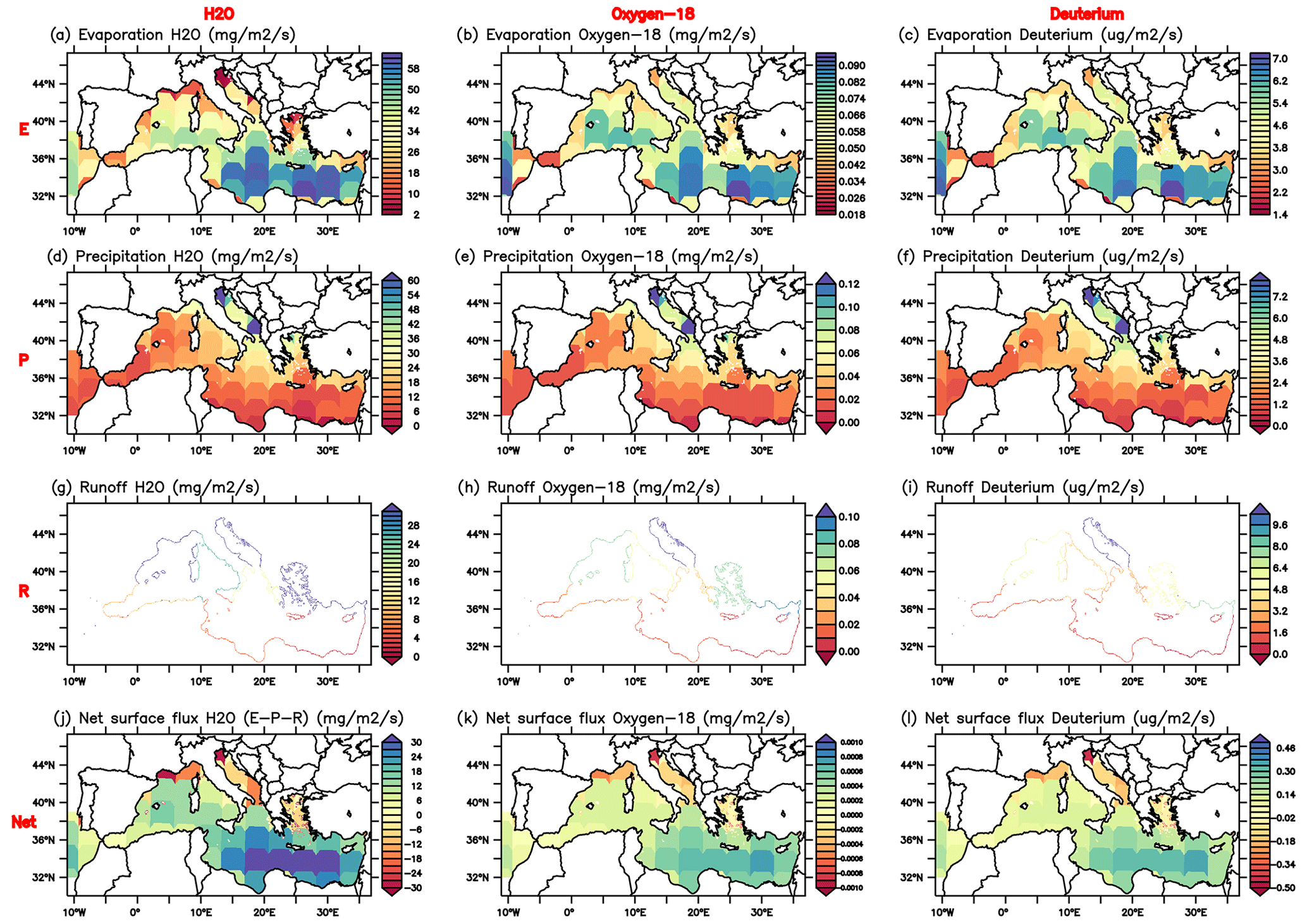
Figure 1 Boundary conditions and input (evaporation and precipitation) maps applied to NEMO that originate from the LMDZ-iso atmospheric model (Risi et al., 2010b). (a) Evaporation, (d) precipitation, (g) river runoff, and (j) net surface flux (E–P–R) for H₂O. (b, e, h, k) The same but for δ¹⁸O_w. (c, f, i, l) The same but for δD_w. The isotopic composition of river runoff is not available from the LMDZ-iso model: this flux is computed as ¹⁸RP ×R, where R is prepared from the data of Ludwig et al. (2009) and Vörösmarty et al. (1996) and ¹⁸RP is the isotopic ratio in precipitation at the same time and location.

Here we force the simulations from the global isotopic atmospheric model LMDZ-iso (Risi et al., 2010b), which is available with two horizontal resolutions; on the coarse latitude–longitude grid R96 (2.5° × 3.75°), the vertical grid of LMDZ-iso extends over 39 layers. The LMDZ-iso atmospheric simulation was conducted following the Atmospheric Model Intercomparison Project (AMIP) protocol, as presented in Risi et al. (2010b), utilising prescribed monthly and interannually varying SST and sea ice, in addition to a constant CO₂ value of 348 ppm for the present-day situation. The impact of these low pCO₂ values in comparison to the current value of 421 ppm is constrained by the fact that the model has been evaluated against in situ data sampled primarily in the 1980s (see Risi et al., 2010b, 2013, for more details on the atmospheric simulation). The aim is to assess the model's performance in the present climate and against in situ data observed between 1982 and 2022. Therefore, we have opted to use the climatological mean of the LMDZ-iso 1990–2020 simulation as boundary conditions. This choice was made to minimise the warming trend during this period and to ensure that the precipitation and evaporation simulated by the LMDZ-iso model for the current climate situation are as close to the average state as possible, with minimal impact from interannual variability. LMDZ-iso simulates the spatial and seasonal variations in both δ¹⁸O and deuterium excess (d-excess = $\mathit{\delta }\mathrm{D}-\mathrm{8}\times {\mathit{\delta }}^{\mathrm{18}}\mathrm{O}$; Dansgaard, 1964) reasonably well. These fluxes were carefully interpolated onto the NEMO-MED12 grid (see Fig. 1). It must be acknowledged that the spatial resolution of LMDZ-iso is relatively coarse for the Mediterranean Sea. It was necessary to use low-resolution forcing on the simulated isotopic composition concentration because no higher-resolution atmospheric isotopic model simulations similar to the dynamical forcing of NEMO-MED12 dynamical simulation (50 km) are available at the moment. We therefore performed some sensitivity tests of the results by changing the horizontal resolution of LMDZ-iso between R96 and R144; the results of these experiences are shown in Appendix C. The impact of this low resolution on the simulated isotopic composition is limited because we used precalculated dynamical fields of the NEMO-MED12 model (in offline mode) forced by a higher-resolution atmospheric model (50 km) ARPERA dataset (Beuvier et al., 2012b; Herrmann and Somot, 2008; Herrmann et al., 2010).

Isotopes are included in the river discharge of the land surface model ORCHIDEE (Risi et al., 2016), but the isotopic version of ORCHIDEE is too old to be coupled with LMDZ-iso. Therefore, as previously done in Delaygue et al. (2000) for the global ocean, we used river discharge estimation from observations and attributed the isotopic composition of precipitation at the river mouth. River inputs are introduced as freshwater sources at river mouths in the surface layer (Fig. 1g, h, i). We used the climatological mean of the interannual dataset of Ludwig et al. (2009) to compute monthly runoff values of the 33 main river mouths covering the entire Mediterranean drainage basin (RivDIS dataset; Vörösmarty et al., 1996). The Nile played a crucial role in freshening surface water during sapropel events. However, since the construction of the Aswan High Dam in 1965, its influence has decreased (Abu El Ella, 1993; Nixon, 2003). As a result, the Nile is no longer a major contributor to the current state of the Mediterranean Sea.

The values of the inputs of the other rivers are averaged in each Mediterranean sub-basin and placed as coastal runoff in each NEMO-MED12 coastal grid point of these sub-basins (Fig. 1g, h, i), as done in Beuvier et al. (2012a) and in Palmiéri et al. (2015). Similarly, since it is difficult to couple the old isotopic version of ORCHIDEE with the current version of LMDZ-iso, we adopt an alternative solution to represent the isotopic flux carried by rivers to the ocean: this flux is calculated as ${\mathcal{R}}_R={\mathcal{R}}_P\times R$, where R is the runoff prepared from the data of Ludwig et al. (2009) and Vörösmarty et al. (1996) (see above) and ℛ_P is the isotopic ratio in precipitation at the same time and location (Fig. 1) as adapted from Delaygue et al. (2000). We have performed some sensitivity simulations to better assess the effect of ∂¹⁸O_river. The results of these experiences are included in the Appendix to further clarify this point (see Appendix E). The exchange with the Atlantic Ocean is performed through a buffer zone between 11° W and the Strait of Gibraltar, where 3-D water isotopes (δ¹⁸O_w and δD_w) and salinity model fields are relaxed to the observations from a global gridded dataset of oxygen isotopic composition in seawater (LeGrande and Schmidt, 2006) and using global model outputs after multiple sensitivity simulations (not shown here).

Let ℰ, 𝒫, and ℛ represent evaporation, precipitation, and runoff, respectively, and then the following boundary condition is relevant at the sea surface.

$$\begin{array}{}\text{(5)}& \mathcal{F}{}^{\mathrm{18}}\mathrm{O}=\mathcal{E}({\mathcal{R}}_{\mathrm{s}}-{\mathcal{R}}_E)-\mathcal{P}({\mathcal{R}}_{\mathrm{S}}-{\mathcal{R}}_P)-\mathcal{R}({\mathcal{R}}_{\mathrm{S}}-{\mathcal{R}}_R),\end{array}$$

where ℛ_S is the isotopic ratio of the oceanic surface and ℛ_E, ℛ_P, and ℛ_R are the isotopic ratios of evaporation (E), precipitation (P), and runoff (R). In our study, we utilised the offline uncoupled mode of NEMO, which employs precalculated dynamics. This mode operates with a fixed volume and explicit fluxes of evaporation, precipitation, and runoff. Alternatively, the online coupled mode of NEMO can be employed to compute dynamic variables (such as circulation fields U, V, and W) in real time. The sea surface elevation and model layer thicknesses are adjusted by the freshwater flux (E–P–R), consequently affecting the model volume. It is essential to ensure that total volume variations accurately correspond to the E–P–R forcing used to drive the isotopic module, thus maintaining the perfect conservation of tracer content.

2.4 Pseudo-salinity in the stand-alone ocean model

The water fluxes from the stand-alone experiments with LMDZ-iso are not identical to those constraining NEMO-MED12. Therefore, δ¹⁸O_w or δD_w computed with the water fluxes obtained with LMDZ-iso would not be consistent with the salinity predicted by NEMO-MED12. For this reason, we compute a “pseudo-salinity” S_w (Delaygue et al., 2000; Roche et al., 2004). This additional passive tracer does not affect ocean dynamics. Its sole purpose is to provide a coherent assessment of the isotopic fields generated by the model. The evolution equation for S_w is given by Eq. (D2) (in Appendix D), where we replace ℛ_s by S_w and where a zero salinity is associated with the water fluxes (i.e. ℛ_E, ℛ_P, and ℛ_R=0 when solving Eq. D2 for S_w). This passive tracer, hereafter called pseudo-salinity, is calculated offline. The basic understanding of these atmospheric fluxes, ℱ¹⁸O and ℱ^S, is that evaporation tends to increase the surface salinity and the ${}^{\mathrm{18}}\mathrm{O}{/}^{\mathrm{16}}\mathrm{O}$ ratio, in contrast to precipitation and runoff. See Appendix D for more details on the concept of pseudo-salinity.

2.5 Datasets of δ¹⁸O_w and δD_w to evaluate the simulation

For comparison with our model results, we used published in situ data in the Mediterranean Sea (https://data.giss.nasa.gov/cgi-bin/o18data/geto18.cgi, last access: 20 August 2024) including those of Epstein and Mayeda (1953), Stahl and Rinow (1973), Pierre et al. (1986), Gat et al. (1996), Pierre (1999), Voelker (2017), and Reverdin et al. (2022). We also used the global gridded dataset of oxygen isotopic composition in seawater from LeGrande and Schmidt (2006) to compare the observed and modelled large-scale oceanic δ¹⁸O_w distribution (i.e. the east–west gradient). While δD_w observations in Mediterranean waters are not as widespread as δ¹⁸O_w, there are some data available in the eastern basin from Gat et al. (1996) and in the western basin from Reverdin et al. (2022) to validate our simulations.

3 Results

3.1 Simulated present-day distribution of δ¹⁸O_w

As a preliminary assessment of our model results, we evaluated the spatial distribution of δ¹⁸O_w in surface waters, zonal vertical sections, and basin average vertical profiles (see Table 2 and Fig. 2) forced by the coarse-resolution version (R96) of the LMDZ-iso model. The EMed is enriched by more than 0.45 ‰ (see Table 2) compared to the WMed. The largest variation in δ¹⁸O_w of the water is simulated in the surface waters with a strong east–west gradient (Fig. 2a); the δ¹⁸O_w value is up to 2 ‰ in the EMed but only 1.55 ‰ in the WMed. This trend reflects the east–west gradient of oceanic evaporation, which distinguishes the higher evaporation in the EMed from that in the WMed (Fig. 1). The δ¹⁸O_w distribution shows a north–south enhancement in the eastern basin (Fig. 2a) with less enriched surface water in the Aegean and Adriatic basins, two regions characterised by active vertical mixing homogenising the water column, and a relatively high contribution of river discharge to this region (e.g. the Po River in the Adriatic basin). The vertical δ¹⁸O_w distributions are well captured by the model, as shown in the west-to-east section and the vertical profile across the Mediterranean (Fig. 2). The intermediate waters (200–800 m depth) form a more homogeneous layer relative to the surface waters. However, the δ¹⁸O_w values decrease towards the west by 0.35 ‰ at most, which is due to gradual dilution by mixing with the deeper water masses and the Atlantic water. The deep water exhibits homogeneous δ¹⁸O_w values similar to the simulated values in the intermediate water, indicating well-ventilated conditions due to active winter convection.

Table 2 Mean, standard deviation, and minimum and maximum values from the model outputs and available in situ data from Epstein and Mayeda (1953), Stahl and Rinow (1973), Pierre et al. (1986), Gat et al. (1996), and Pierre (1999) calculated in the surface water (0–100 m depth) of the whole basin and the eastern and western basins.

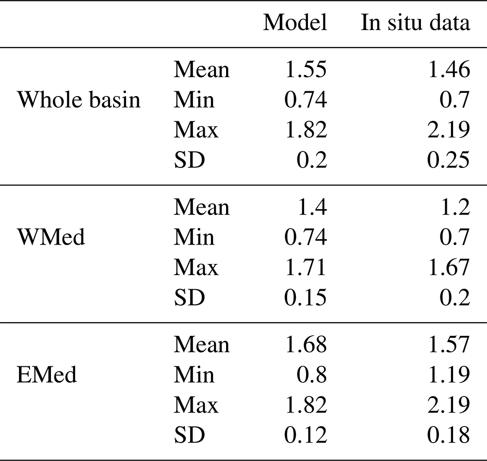
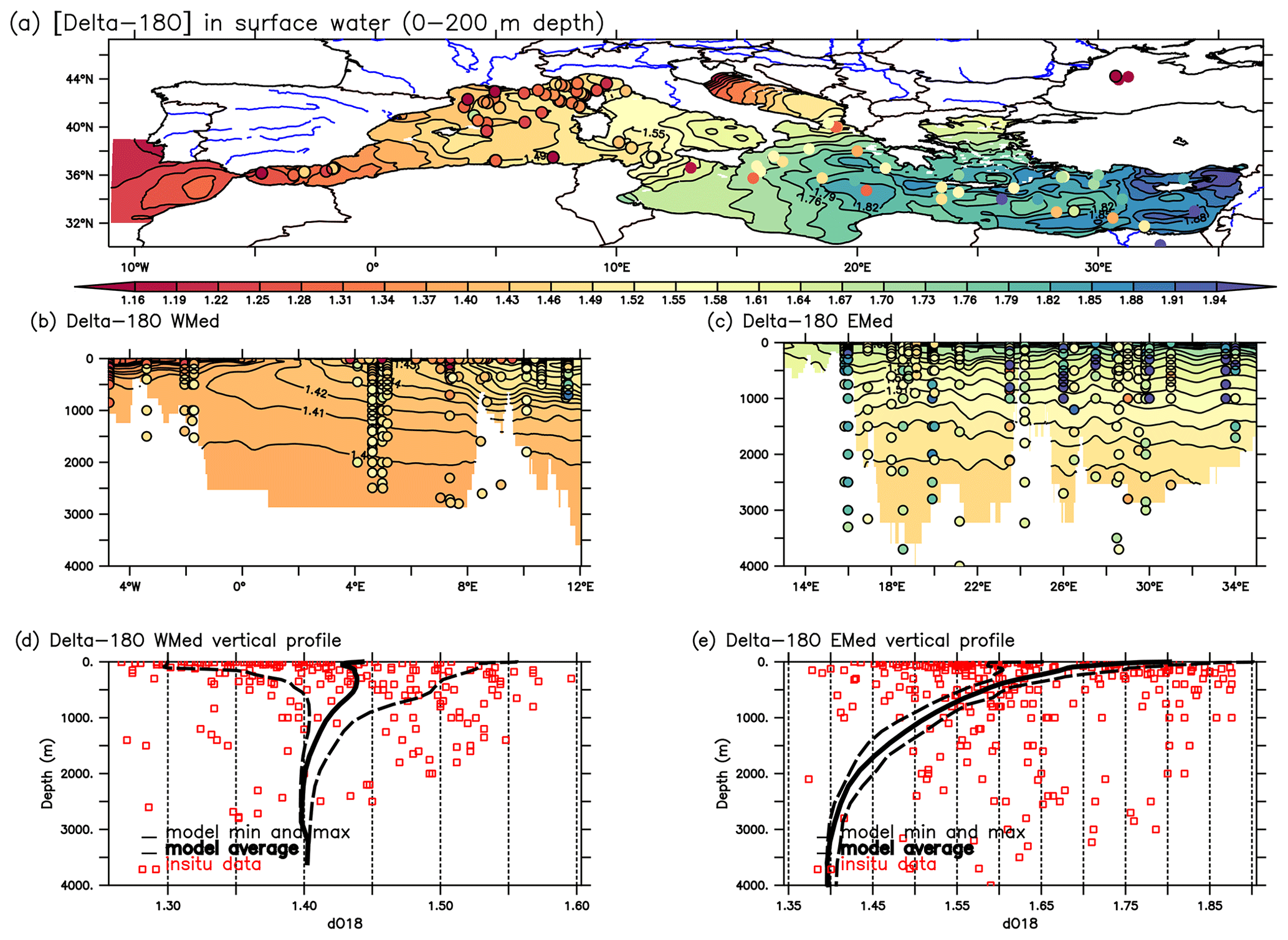
Figure 2 The model outputs against in situ data for the present-day situation. (a) δ¹⁸O_w (in ‰) distribution in the surface water (50 m depth). (b) E–W vertical section of δ¹⁸O_w (in ‰) in the western Mediterranean basin. (d) Zonal mean comparison of δ¹⁸O_w (in ‰) average vertical profiles in the western basin presenting model results against in situ data. (c, e) The same as (b) and (d) but for the eastern basin. Colour-filled dots represent in situ observations from Epstein and Mayeda (1953), Stahl and Rinow (1973), Pierre et al. (1986), Gat et al. (1996), Pierre (1999), Voelker (2017), and Reverdin et al. (2022). Both the model and in situ data use the same colour scale.

Comparison of the model output with in situ data shows that the model reproduces the observed east–west gradient that characterises the surface waters well (Fig. 2a, Table 2) and correctly reproduces the zonal gradients observed in the intermediate and deep waters (Fig. 2b, c). The simulated mean vertical profile of δ¹⁸O_w is consistent with the observations in the western basin of δ¹⁸O_w values (Fig. 2d). The spreading of Atlantic water in the surface of the Alboran basin is well reproduced in the simulation (Fig. 2a, 2d). In the eastern basin, the highest value of δ¹⁸O_w is well reproduced in the simulation, but the model largely underestimates the mean values of the observations in the intermediate and deep waters (Fig. 2c, e). This offset is related to the weak formation of the simulated EMDW in the Adriatic sub-basin, as already noted by Ayache et al. (2015a) and Palmiéri et al. (2015). To further evaluate the relationship between the in situ data and the simulated δ¹⁸O_w, the longitudinal distribution of δ¹⁸O_w is examined for each basin (Fig. 3b, c). A pronounced longitudinal gradient is found for simulated and observed δ¹⁸O_w values, with more enriched values in the EMed (between 27 and 36° E), more depleted values in the WMed (between −6 and 11° E), and an intermediate value in the central basin (Fig. 3b, c). The observed salinity agrees well with the simulated pseudo-salinity results (Fig. 3), in contrast to the highly variable in situ δ¹⁸O_w values.

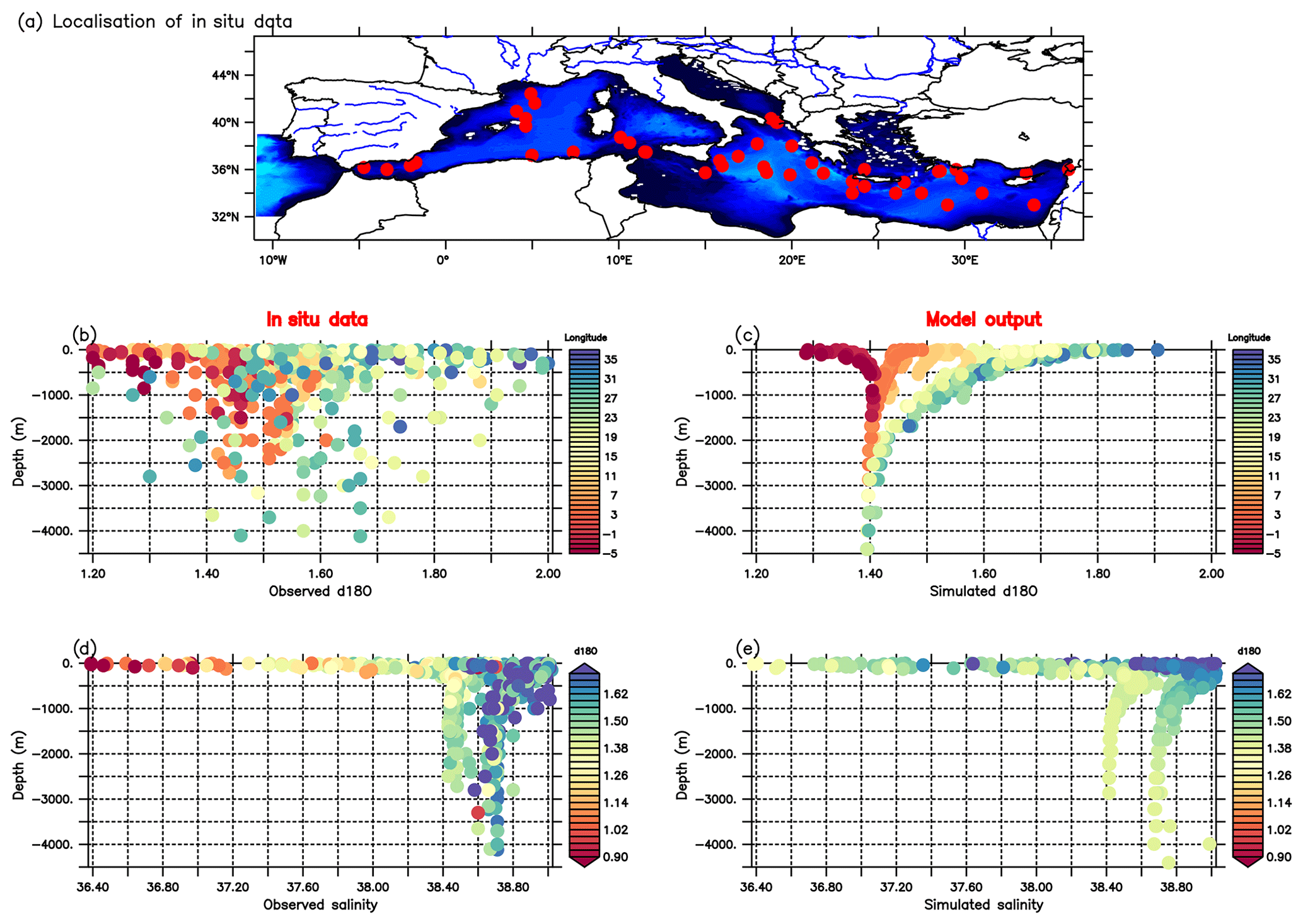
Figure 3 (a) Location map of all stations of in situ data (Epstein and Mayeda, 1953; Stahl and Rinow, 1973; Pierre et al., 1986; Gat et al., 1996; Pierre, 1999). (b) Depth profiles of δ¹⁸O_w (in ‰) from in situ data (the colour code indicates the longitude of the data in ° E). (c) The same as in (b) but from the model output. (d) Depth profiles of salinity from in situ observations (the colour code indicates the δ¹⁸O_w for each data station). (e) The same as in (d) but from the model output.

3.2 The δ¹⁸O_w–salinity relationship in the Mediterranean waters

The lower two panels in Fig. 3 show the depth profiles of salinity in relation to δ¹⁸O_w from in situ data (Fig. 3d) and model output (Fig. 3e) forced by the coarse-resolution version (R96) of the LMDZ-iso model. The more evaporated water in the eastern basin (pseudo-salinity up to 38.9) matches well with more enriched water (δ¹⁸O_w above 1.98 ‰), especially at intermediate depths (300–700 m) corresponding to the LIW layer. The decrease in δ¹⁸O_w and salinity in the deep water is well captured by the model (Fig. 3c, d, e). However, the model tends to overestimate the value of δ¹⁸O_w associated with a lower salinity in the WMed (salinity = ∼ 36.4), i.e. the salinity of the inflowing Atlantic waters (Fig. 3c and e).

To further analyse the relationship between δ¹⁸O_w and salinity, we plot the regression slope of δ¹⁸O_w versus salinity for the available in situ data (Fig. 4a, b, c) and from the model output (Fig. 4 d, e, f). There is a significant positive correlation between salinity and δ¹⁸O_w from the model results (r²= 0.82) and from the in situ data (r²=0.60) for the whole Mediterranean Sea. The EMed shows the weakest correlation between salinity and δ¹⁸O_w (r²=0.20, Fig. 4c). The whole set of in situ data values measured in the Mediterranean waters defines the following linear equation: δ¹⁸O_w = 0.29S−9.46 (Fig. 4a); the equation becomes δ¹⁸O_w = 0.26S−8.60 in the WMed and δ¹⁸O_w = 0.25S−8.19 in the EMed (Fig. 4b, c). The difference between the two equations remains fairly small, with a similar slope in the EMed and different intercepts. The model simulated a similar slope to in situ data throughout the basin (δ¹⁸O_w = 0.25S−8.01), and the zonal trend is comparable to observation (0.25 and 0.26 for the WMed and the EMed, respectively; Fig. 4e and f). Pierre (1999) estimated a similar slope (0.25) for the whole Mediterranean water and 0.27 in the Alboran basin (western basin). Figure 5a displays the temporal distribution of the δ¹⁸O_w–salinity slope in Mediterranean surface water, computed using simulated climatology over the last 30 years. Low values (around 0.3, Fig. 5) as well as a weak correlation (0.24, Fig. 4f) were calculated in the eastern basin. The lower slopes reflect the impact of the evaporation surplus in the EMed (Voelker et al., 2015). High values of the slope are simulated in the western basin (>0.5, Fig. 5a), especially in the Alboran basin, which is influenced by Atlantic water characterised by a δ¹⁸O_w–S slope of 0.48 (Laube-Lenfant, 1996; Pierre, 1999), and 0.32 obtained by Voelker et al. (2015) in the northeastern Atlantic with a strong bias towards subtropical waters. While this simulated longitudinal trend appears to agree with observations (Figs. 4 and 5), it is important to note that there are some additional longitudinal variations in slope, particularly in the Aegean Sea and southeasternmost part of the Levantine basin. Figure 5b displays the spatial δ¹⁸O_w–salinity slope from the model outputs. For each grid point, it is computed as the slope of the δ¹⁸O_w relative to salinity linear regression, based on the simulated surface values from the 12 surrounding grid points. The mean slope of the spatial regression (∼ 0.3) is relatively similar to the mean value of temporal regression (Fig. 5a). However, the slope based on spatial regression shows greater variation, mainly due to the oceanic circulation, particularly in areas of high mesoscale activity (i.e. the Algerian and Levantine basins), with potentially greater transport and change in salt and water content in the water column caused by the oceanic mesoscale eddies.

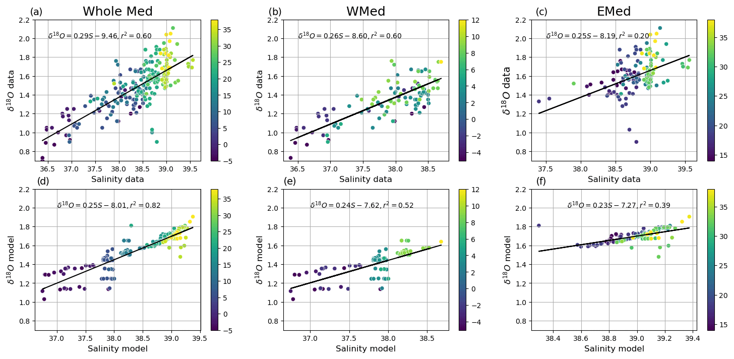
Figure 4 δ¹⁸O_w–salinity relationship in the surface water (average 0–200 m depth of the whole basin – a, d; western basin – b, e; and eastern basin – c, f) calculated from available in situ data (Epstein and Mayeda, 1953; Stahl and Rinow, 1973; Pierre et al., 1986; Gat et al., 1996; Pierre, 1999) in the upper panel (in a–c) and from model outputs extracted in the same positions of in situ data (in d–f). The colour code indicates the longitude of the data in degrees east (° E).

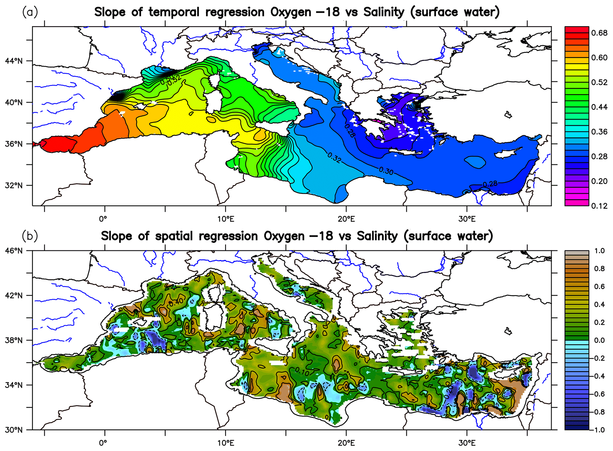
Figure 5 (a) Horizontal map of the slope of temporal regression between the δ¹⁸O_w–salinity in the surface water computed using simulated climatology of the last 30 years. (b) Spatial δ¹⁸O_w–salinity slope from the model outputs calculated for each grid point using simulated surface values from the 12 surrounding grid points. The non-significant zones for the regression at the 95 % level are masked.

3.3 Present-day distribution of deuterium (δD_w) and d-excess

Since identical boundary fluxes (precipitation, evaporation, and river runoff) drive both δ¹⁸O_w and δD_w isotopes in the surface water, the zonal gradient patterns between the EMed and WMed are strikingly similar (Fig. 6), with the most enriched areas (δD_w values ≥ 8 ‰) located in the more evaporated EMed and the most depleted areas in the WMed (especially the Alboran basin with δD_w values ≤ 6 ‰). As with δ¹⁸O_w, the δD_w values are lower in the Aegean basin, which may be related to a relatively high freshwater contribution (P and R) and active vertical mixing. The spatial structures of δD_w simulated by the model are consistent with the observations available in the EMed and in the WMed surface water (Fig. 6), with values slightly lower than in situ data in the surface and intermediate waters. The distributions are more uniform in the deep water. Simulated δD_w exhibit a linear relationship with δ¹⁸O_w (Fig. 7a) and salinity (Fig. 7b) with a significant correlation (r²=0.98 and 0.94, respectively). δD_w observations in the Mediterranean are not as extensive as those of δ¹⁸O_w. Therefore, there are currently not enough data to constrain and validate our δD_w simulation, as shown in Fig. 7c, where a weak correlation (r²=0.25) was found between the few data available in the eastern basin and δD_w simulated in the same data location.

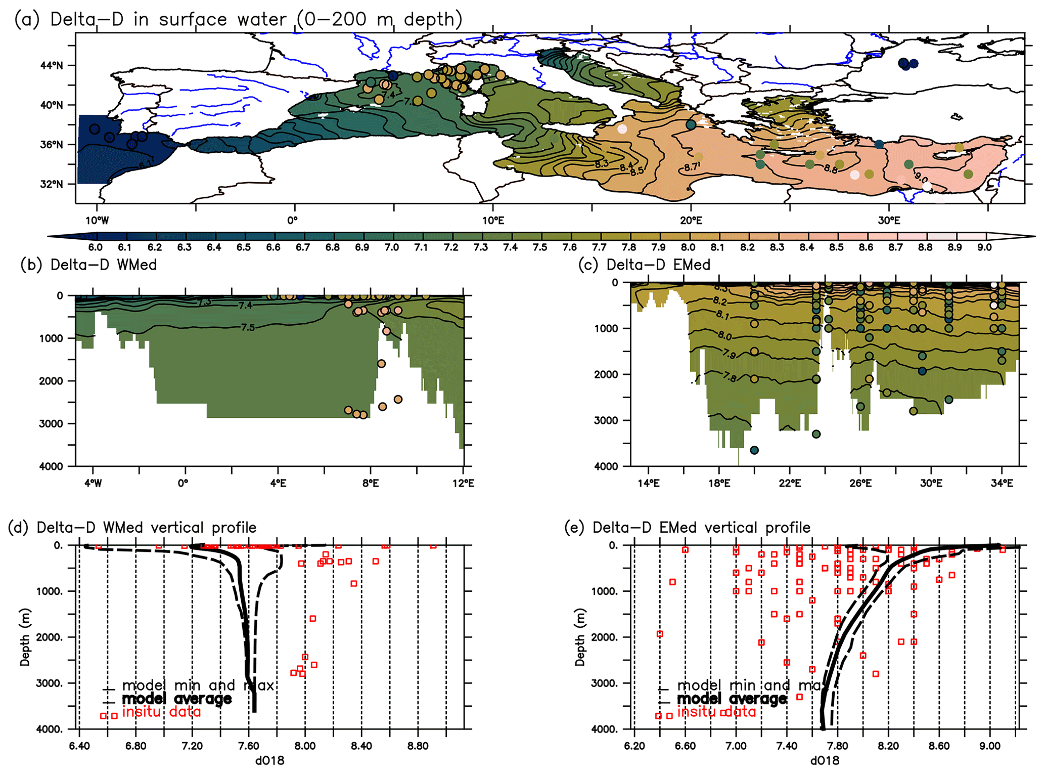
Figure 6 The same as in Fig. 2 but for the deuterium isotope (in ‰). In situ data from Gat et al. (1996) and from Reverdin et al. (2022).

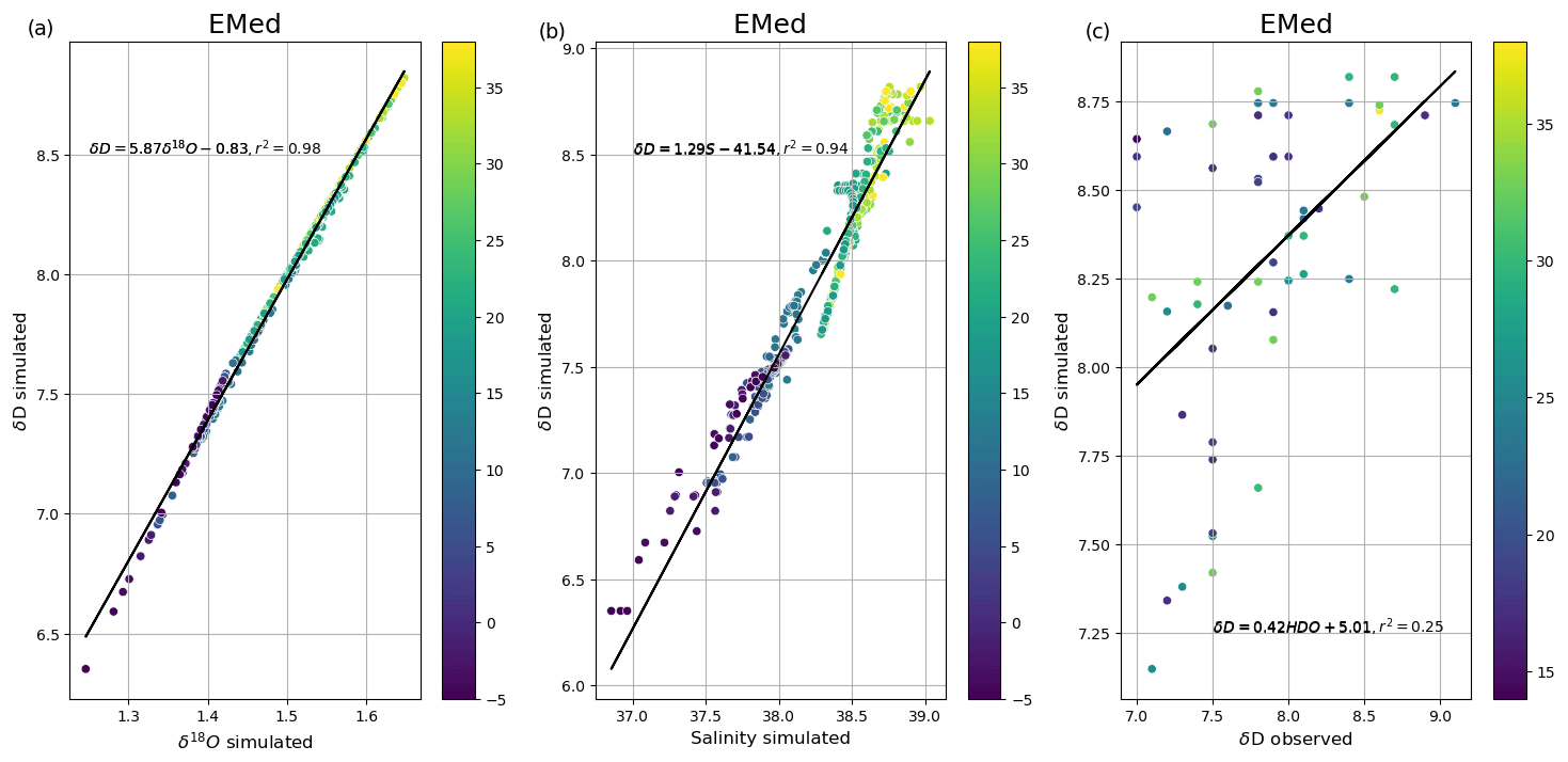
Figure 7 Multi-scatterplot of simulated δ¹⁸O_w (averaged over the last 30 years of the simulation) versus simulated δD_w at the same location of in situ data in the eastern basin (a), simulated salinity versus simulated δD_w (b), and observed δD_w (from Gat et al., 1996) against simulated δD_w (c). The colour code indicates the longitude of the data in degrees east (° E).

The deuterium excess, “d-excess”, reflects the relationship between the isotopic ratios of hydrogen and oxygen. This indicates the kinetic (non-equilibrium) fractionation effects that occur when water evaporates from oceanic regions (Dansgaard, 1964). The simulated mean surface water d-excess values range from −4.4 ‰ to −1.5 ‰, with relatively small variations (variance = −0.27 ‰), and a clear negative shift in simulated d-excess values was observed across the basin (Fig. 8). The WMed is enriched in d-excess compared to the EMed, and the regions with the lowest d-excess are located in the Levantine sub-basin. In situ observations of d-excess from Gat et al. (1996) and Reverdin et al. (2022) show an important E–W gradient, with higher values recorded in the western Mediterranean basin (WMed) and lower values in the eastern Mediterranean basin (EMed). The simulated D-excess values closely match the in situ data from the EMed, whereas the model significantly underestimates observed δD_w values in the WMed (Fig. 8). The model results show an increase in d-excess for water masses with higher δ¹⁸O_w depletion, as suggested by Xu et al. (2012) using the model MPI-OM simulating water isotope variation on a global scale. These negative values are generally in accordance with the positive values of deuterium excess in atmospheric water vapour and precipitation observed and simulated in this region, associated with the dryness of near-surface air (Pfahl and Wernli, 2008). In a more recent study, Benetti et al. (2014) observed d-excess ranging from −1.56 to −1.72 in the surface waters of the eastern subtropical Atlantic. Their findings reveal a contrasting trend between increasing δ¹⁸O_w and δD_w and decreasing d-excess, which corresponds closely with our simulated values. The authors suggest that d-excess variations are predominantly influenced by humidity and wind speed rather than mixing effects.

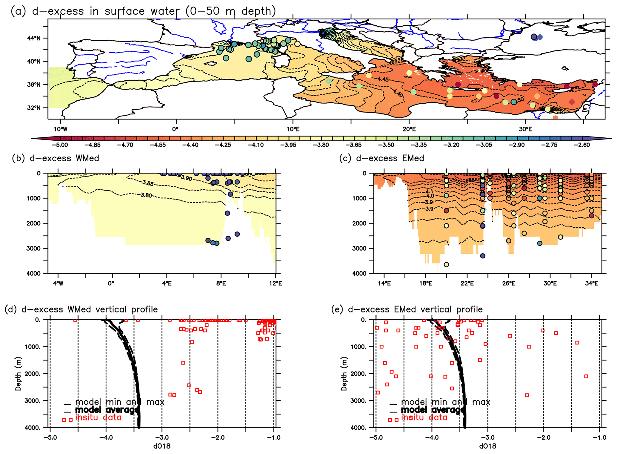
Figure 8 The same as in Figs. 2 and 6 but for the d-excess in the surface water defined as deuterium excess (d-excess = δD_w − 8×δ¹⁸O_w; Dansgaard, 1964). Colour-filled dots represent in situ observations from Gat et al. (1996) and Reverdin et al. (2022).

3.4 Variations in δ¹⁸O_calcite in the Mediterranean Sea

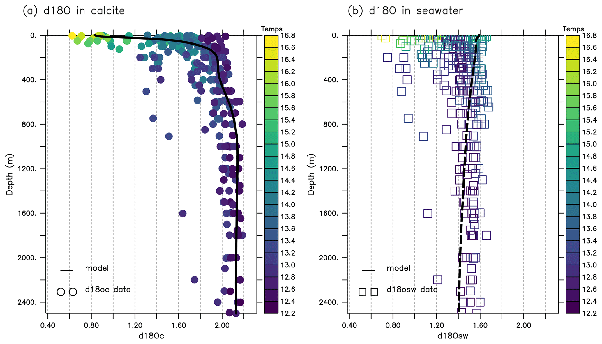
A useful tool for reconstructing past climate is the isotopic composition of foraminiferal shells from sediment cores (Shackleton, 1967). However, due to temperature-dependent fractionation, the isotopic signature of the CaCO₃ shell (δ¹⁸O_c) differs from that of δ¹⁸O_w. The δ¹⁸O_c values depend on both δ¹⁸O_w and seawater temperature at calcification depth. For planktonic foraminifera, the isotopic fractionation relationships during calcification can be assumed to be represented by an equation for equilibrated calcite. We used a paleotemperature equation for inorganic calcite by Kim and O'Neil (1997) modified by Bemis et al. (1998), with the use of the 0.27 ‰ correction from VSMOW (Vienna Standard Mean Ocean Water) to VPDB (Vienna Pee Dee Belemnite) conversion. The equation was applied to both the model output and the available in situ data, as presented in Sect. 2.5.

$$\begin{array}{}\text{(6)}& {\displaystyle }\mathcal{T}=\mathrm{16.1}-\mathrm{4.64}({\mathit{\delta }}^{\mathrm{18}}{\mathrm{O}}_{\mathrm{c}}-{\mathit{\delta }}^{\mathrm{18}}{\mathrm{O}}_{\mathrm{w}})+\mathrm{0.09}({\mathit{\delta }}^{\mathrm{18}}{\mathrm{O}}_{\mathrm{c}}-{\mathit{\delta }}^{\mathrm{18}}{\mathrm{O}}_{\mathrm{w}}{)}^{\mathrm{2}}\text{(7)}& {\displaystyle }\begin{array}{rl}{\mathit{\delta }}^{\mathrm{18}}{\mathrm{O}}_{\mathrm{c}\left({\mathrm{VPDB}}_{\mathrm{‰}}\right)}& =({\mathit{\delta }}^{\mathrm{18}}{\mathrm{O}}_{\mathrm{w}\left({\mathrm{VSMOW}}_{\mathrm{‰}}\right)}-\mathrm{0.27})\\ & +{\displaystyle \frac{\mathrm{4.64}-\sqrt{\mathrm{21.53}-\mathrm{0.36}(\mathrm{16.1}-{\mathcal{T}}_{\mathrm{°}\mathrm{C}})}}{\mathrm{0.18}}}\end{array}\end{array}$$

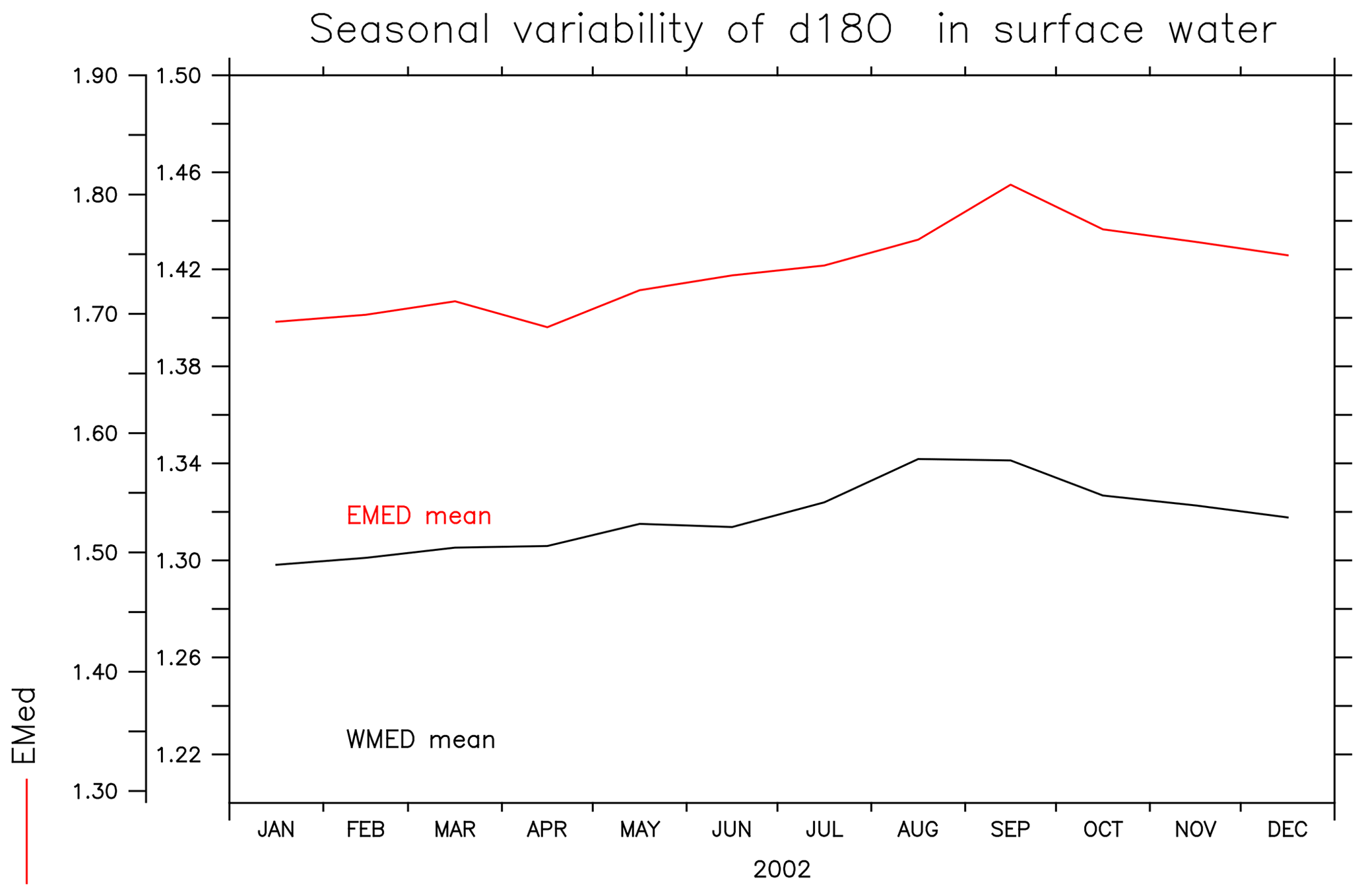
The relationship of δ¹⁸O_c with temperature and the influence of seasonality are shown in Fig. 9. The mean annual δ¹⁸O_c values for surface seawater were computed using the model outputs of surface δ¹⁸O_w and surface water temperature. The simulated annual mean δ¹⁸O_c values vary from −0.8 to 2 ‰ at the surface (Fig. 9b), with higher values in the northern part of the Mediterranean and lower values near the southern coast. This latitudinal gradient of δ¹⁸O_c is different from the zonal pattern of δ¹⁸O_w (Fig. 2a) and is related to the effect of temperature (Fig. 9c). Considering this strong temperature dependency, the seasonal variability in δ¹⁸O_c was examined (Fig. 9d). The highest simulated δ¹⁸O_c values were obtained for winter (February, March) and the lowest values for summer and autumn. The δ¹⁸O_c values calculated from in situ δ¹⁸O_w and measured seawater temperature show the same seasonal trend (Fig. 9e). Even though the available observational data do not cover all the months of the year, our results indicate the importance of temperature effects on δ¹⁸O_c in the Mediterranean Sea. We note here that seasonal variation in δ¹⁸O_w is small in the surface layer of both the eastern and the western basins (see Fig. A1 in the Appendix). The δ¹⁸O_c variation is mainly localised in the surface and intermediate waters (first 300 m depth) (Fig. A2 in the Appendix). The comparison of simulated and observed δ¹⁸O_c (0–50 m depth) shows a strong positive correlation with a similar range of variability (between −0.22 and 1.91 ‰ from the model output and between −0.82 and 1.97 from the in situ data) to that shown in Fig. 9f. In this study, we analysed the impact of temperature on δ¹⁸O_c calculations, both in a global model and at high regional resolution. Please refer to Appendix B for further details.

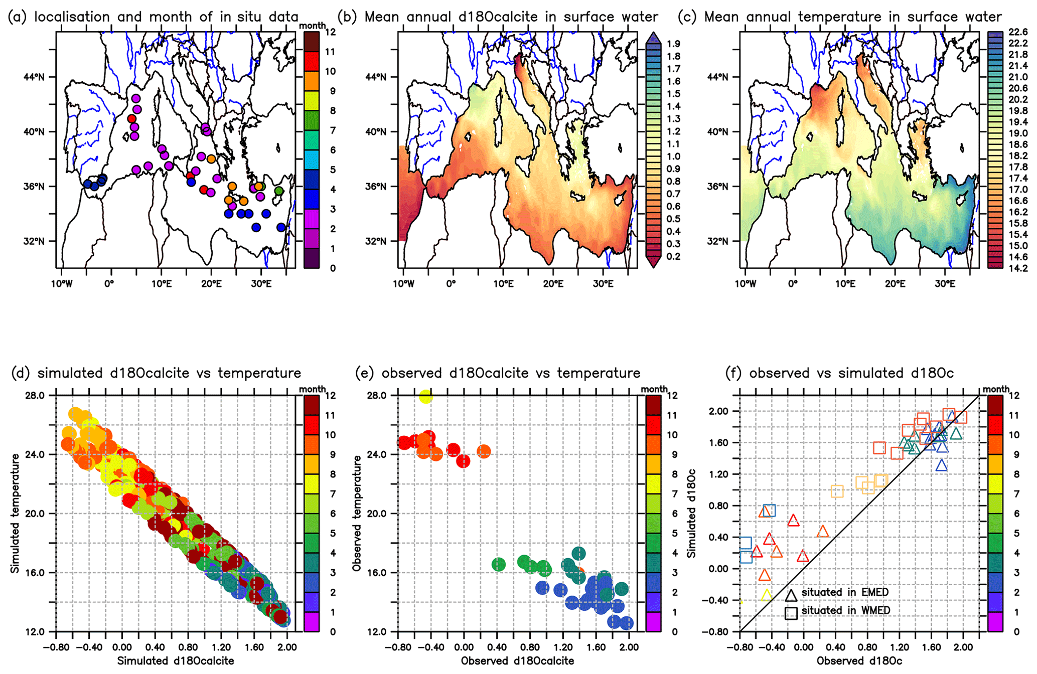
Figure 9 (a) Localisation and the month of available in situ data. (b) Annual mean δ¹⁸O_c (in ‰) distribution in calcite (surface layer 0–100 m depth), calculated using the method of Bemis et al. (1998). (c) Horizontal maps of surface mean annual temperature in degrees Celsius (°C). (d) Multi-scatterplots of simulated δ¹⁸O_c against simulated temperature in the same location; the colour code shows months. (e) The same as (d) but from in situ data. (f) Comparison of the simulated and observed δ¹⁸O_c (in ‰) in the surface layer averaged in the two basins (squares represent the WMed, triangles the EMed, and the solid line the model). The colour code shows months.

4 Discussion

This study provides the first simulation of the water isotopes (δ¹⁸O_w and δD_w) in the Mediterranean Sea covering the entire basin. These two tracers were implemented in the high-resolution regional model NEMO-MED12. New insights into the distribution of water isotopes and their relation to salinity in the Mediterranean Sea were obtained by comparing this numerical study with in situ data. Analysis of the results from an oceanic point of view shows good agreement with the in situ data, opening up a range of possibilities for long-term paleoclimate simulations in this basin and the use of this modelling approach in coupled ocean–atmosphere models. The inputs and boundary conditions δ¹⁸O_w and δD_w were taken from a global atmospheric model with a low resolution and have been tested for the first time in this study with a regional model at a high resolution. Both observed δ¹⁸O_w and observed δD_w show a pronounced east–west gradient, characterised by more enriched water in the eastern basin than in the western basin. This gradient is well captured by the model and is in good agreement with the available in situ data. It is not possible to constrain and validate the δD_w simulation due to the limited number of δD_w observations. Thus, our discussion below focuses on the results of the δ¹⁸O_w simulation.

A significant correlation between model output and in situ data (r²=0.68) was obtained over the whole basin, with a higher correlation in the WMed than in the EMed. Our model also successfully simulates the observed vertical distribution of the water isotope composition of the Mediterranean water masses (Figs. 2, 6). Despite a slight bias in the EMed due to the previously reported weak formation of AdDW, the vertical distribution compares favourably with the available in situ data. Some improvements are still needed in certain aspects of the simulation. The model largely underestimated the mean δ¹⁸O_w values of observations in intermediate and deep waters and failed to simulate the highly enriched water in the eastern basin (up to 2.4 ‰ by Gat et al., 1996). This inconsistency should be investigated in a fully coupled ocean–atmosphere model with a higher horizontal and vertical resolution of the atmospheric model. The advantage of using a coupled model lies in the consistent simulation of changes in the different components of the model (for instance between the precipitation over land, the ocean variability, and runoff input from the land) and more realistic ocean–atmosphere feedbacks in the coupled model (Bretherton and Battisti, 2000; Schmidt et al., 2007).

The main difference between the data and the numerical simulations is the smaller amplitude of δ¹⁸O_w, particularly in the eastern basin. This discrepancy can be explained in two ways. First, this may be due to the low spatial resolution of the isotope forcing. Vadsaria et al. (2020) showed that high resolution (∼ 30 km of the atmospheric model) is critical to accurately capture the synoptic variability needed to initiate the formation of the intermediate and deep waters of the Mediterranean thermohaline circulation. Due to the peculiarities of the atmospheric circulation (high wind gusts in winter) and the oceanic circulation (deep convection) in this intercontinental basin, high-spatial-resolution forcings are needed (Li et al., 2006). Nevertheless, a change in the horizontal resolution of the LMDZ-iso atmospheric model (from R96 to R144) does not improve the model results, and the model does not simulate the highest values of δ¹⁸O_w observed by Gat et al. (1996) in the eastern basin at either resolution. There may be a certain threshold of spatial resolution below which the simulation is improved by a finer resolution. Unfortunately, LMDZ-iso simulations at resolutions finer than R144 are not yet available to test this hypothesis. Sensitivity tests were performed to investigate the effect of changing the resolution of the LMDZ-iso atmospheric model (between R96 and R144) and the oceanic model (between ORCA2 and NEMO-MED12), the results of which are presented in the Appendix of this paper (see Appendix C).

The second hypothesis is that the discrepancy is due to the physics of the atmosphere, which is independent of the horizontal resolution. In parallel with the δ¹⁸O_w that is too low in the western part of the basin, LMDZ-iso underestimates the depletion and d-excess of precipitation and vapour in this region (Risi et al., 2010a). These discrepancies in LMDZ-iso are consistent with the insufficient near-surface air dryness. The underestimated dryness would lead to a lower surface evaporative flux in LMDZ-iso, leading NEMO-MED12 to underestimate evaporative enrichment of surface water. In addition, the underestimation of water vapour depletion in the LMDZ-iso leads to an overestimation of evaporative flux (Craig and Gordon, 1965), which in turn leads to a further underestimation of evaporative enrichment of surface water by NEMO-MED12. The underestimation of the dryness in LMDZ-iso could be due to an insufficient vertical resolution (Risi et al., 2012) or to a misrepresentation of shallow convection in this region (Hourdin et al., 2015). Such a discrepancy is not observed in the salinity data. To obtain larger spatial coverage, we used δ¹⁸O_w obtained in the 1971–1990 period in addition to two data points acquired in 1949. Therefore, it is not impossible that temporal variation in δ¹⁸O_w and different data quality with time could induce further scatter. Despite the smaller range of the δ¹⁸O_w values, our parameterisation produced realistic general features of spatial distribution, particularly zonal trends in surface water. The results suggest that this approach can be used to generate water isotopic simulations with adequate validity at decadal timescales (i.e. 50 years of simulation), opening up the prospect of simulations at longer timescales in the context of paleoclimate studies.

Mediterranean regional climatic conditions (i.e. excess of evaporation compared to precipitation) shape a specific relationship in surface waters between observed salinity and δ¹⁸O_w values, characterised by a δ¹⁸O_w–S slope of 0.25, which is much lower than the slope value of 0.45 obtained in Atlantic surface waters (Pierre, 1999) and of 0.32 calculated by Voelker et al. (2015) in the NE Atlantic. Our results are consistent with these findings: δ¹⁸O_w shows a linear relationship with salinity, and the simulated slope of δ¹⁸O_w with salinity (0.28) is very similar to that calculated by Pierre (1999) using in situ observations. The model simulated similar differences between the EMed and the WMed, with a steeper slope in the WMed as computed using in situ data. It is not surprising that there is a high correlation between these two fields, since the processes that affect δ¹⁸O_w at the surface are also those that affect surface salinity. Nevertheless, especially in areas of high mesoscale activity (e.g. the Algerian Basin), the spatial slope δ¹⁸O_w–S of our simulation shows strong variations. The slope is therefore not homogeneous but depends on the local climate conditions (wind speed, temperature, etc.). It is well documented that mesoscale eddies can transport water, heat, salt, and other tracers as they spread in the ocean, influencing water column properties and biological activities (Chelton et al., 2011; Dong et al., 2014). In summary, our simulation results indicate a significant deviation in the slope of the ¹⁸O_w–salinity relationship compared to the global slope (Pierre, 1999; Voelker et al., 2015). The calculated slopes are consistently lower within this basin, reflecting the influence of evaporation surplus, as highlighted by Gat et al. (1996) in their study of the eastern Mediterranean basin.

The simulated δD_w–δ¹⁸O_w relationship provides a realistic d-excess surface field. A full comparison between data and the model is not possible due to the lack of d-excess field data for the Mediterranean. However, the modelled d-excess is consistent with other modelling studies (e.g. Xu et al., 2012) which show an increase in d-excess for water masses more depleted in δ¹⁸O_w. Our simulations show similar negative d-excess values for the whole Mediterranean basin. Thus, assuming that the atmospheric d-excess signature is largely dominated by non-equilibrium isotope fractionation during evaporative processes of marine surface waters (Dansgaard, 1964; Gat et al., 1994), the remaining surface waters should have a negative d-excess value as simulated by our model. More recently, Benetti et al. (2014) observed a contrasting trend between increasing ¹⁸O_w and δD_w and decreasing d-excess, suggesting that d-excess variations are predominantly influenced by humidity and wind speed rather than mixing effects. Simulating both δD_w and ¹⁸O_w is useful for paleoclimate applications involving both δD and ¹⁸O of natural archives, particularly when using this modelling approach in a fully coupled configuration. Notably, δD_w in leaf waxes (Sachse et al., 2015) and speleothem fluid inclusions (van Breukelen et al., 2008) is useful for paleoclimate reconstructions.

An interesting tool for mapping potential changes in the oceanic circulation over time could be a data–model comparison exercise for the δ¹⁸O of calcite in past climates. We can calculate δ¹⁸O_c and compare our model results with δ¹⁸O_c calculated from in situ data, since water temperatures and δ¹⁸O_w are explicitly simulated by our model (see Sect. 3.4). The results show that the surface δ¹⁸O_c distributions derived from the model results are consistent with the general spatial pattern of δ¹⁸O_c measurements in the present-day situation. Higher values of δ¹⁸O_c are simulated mainly in the northern part of the Mediterranean as compared to the southern part. The difference between δ¹⁸O_w and δ¹⁸O_c is related to the Mediterranean temperature pattern, with a high negative correlation, especially in the surface layer. Calcite δ¹⁸O_c is widely used in paleoclimate research. Understanding its seasonal variability is crucial for reconstructing past climates. The influence of seasonal temperature variability on δ¹⁸O_c (Eq. 6) is important, particularly in the Mediterranean Sea because of marked seasonal thermal contrast. The δ¹⁸O_c values are determined by both δ¹⁸O_w and the seawater temperature at the calcification depth. For planktonic foraminifera such as Globigerinoides ruber and Globigerina bulloides, the calcification depth typically ranges from 0 to 100 m, though variations exist depending on the basin (Coppa et al., 1980; Grazzini et al., 1986). The season of maximal foraminiferal production can be estimated by data from sediment traps. For instance, G. ruber and G. bulloides have been associated with calcification seasons in October–November and April–May according to Kallel et al. (1997), while others suggest January–March (Avnaim-Katav et al., 2019) and February–April (Rigual-Hernández et al., 2012). In this context, we used our model results to explore the relationship between δ¹⁸O_c and temperature. We employed a paleotemperature equation for inorganic calcite by Kim and O'Neil (1997), modified by Bemis et al. (1998), as shown in Fig. 9. Our simulations indicate that the highest δ¹⁸O_c values occur during winter (February, March), while the lowest values are observed during summer and autumn. Although the available observational data do not cover all months of the year, our results align with existing data, highlighting the significant influence of temperature on δ¹⁸O_c in the Mediterranean Sea. Nonetheless, a dedicated study should be conducted to further elucidate the seasonal aspect.

To extend this study, certain sensitivity tests and modelling developments must be performed. For the present-day situation, it would be useful to evaluate the influence of different forcing factors on the distribution of water isotopes in the Mediterranean (the influence of the inflow–outflow from the Atlantic at the Strait of Gibraltar, the influence of surface runoff, etc.). In our experimental set-up, river runoff is computed by considering the isotopic signature of precipitation. This assumption can lead to an unrealistic isotopic composition of the river runoff. Future studies will improve the representation of water isotopes in river runoff using a coupled ocean–atmosphere–land model. For past climates such as during the Holocene (i.e. sapropel events), appropriate oceanic circulation and atmospheric fluxes could be combined to estimate differences from the present-day situation. This could help to test and better understand the reconstructed past data. The use of transient simulation offers an interesting test bed to make progress on this issue, especially to evaluate the Mediterranean circulation sensitivity to hydrological and thermal perturbation during the most recent Holocene sapropel S1 (10.5 to 6.1 ka cal BP) and the last interglacial sapropel S5 (128–122 ka; Grant et al., 2016), which occurred under warm conditions with strong seasonality and a high sea level stand. Regional climate models can bridge the gap between the coarse resolution of global climate models and the regional to local scales. They provide a more realistic representation of physical processes and climate feedback compared to global climate models. This is especially true for the Mediterranean region with its complex geology (Li et al., 2006). The water isotope modelling package presented in this study can be used in coupled regional configurations, such as RegIPSL (Drobinski et al., 2012), which may assist in the preparation of a global-scale coupled version. Additionally, a sequential architecture of a global–regional modelling platform has been developed by Vadsaria et al. (2020) using the same dynamical model, NEMO-MED. This platform can be used sequentially in a wide range of paleoclimate contexts, from the Quaternary to the Pliocene, with a regional model that is forced by a global model.

5 Summary and conclusions

Here, for the first time, stable water isotopes were successfully implemented in a high-resolution regional model of the Mediterranean (called NEMO-MED12-watiso v1.0) forced by the atmospheric model LMDZ-iso. The isotopic composition of seawater δ¹⁸O_w and δD_w is simulated explicitly by the oceanic model. The model successfully simulates the observed basin-scale pattern of δ¹⁸O_w and E–W gradients in surface water, evidencing the larger degree of evaporation of surface waters in the eastern basin. It also successfully reproduces the vertical distribution of δ¹⁸O_w in Mediterranean water masses. Furthermore, the simulated δ¹⁸O_w–salinity relationships are also in good agreement with the data, with a smaller slope in the EMed than in the WMed and a slope of 0.25 across the basin. The modelled d-excess values are in good agreement with other modelling studies, with an enhancement of d-excess for water masses depleted in δ¹⁸O_w. Such negative d-excess values are found throughout the Mediterranean Sea in our simulation results. We examine the relationship of δ¹⁸O_c with temperature and the influence of seasonality. The gradient of δ¹⁸O_c is different from the pattern of δ¹⁸O_w due to the effect of temperature, with the highest values obtained in winter and the lowest values in summer and autumn.

Improvements are needed in certain aspects of the simulation. A global atmospheric model simulation (LMDZ-iso) with a relatively coarse resolution was used for the isotopic forcing fluxes of precipitation and evaporation. In order to generate steeper gradients in the hydrological-cycle variables over the Mediterranean basin (evaporation, precipitation) and to improve the isotopic simulation of the present study, a higher spatial resolution (<50 km) may be required. Here we calculate the isotopic composition of rivers based on the isotopic composition of precipitation, which means that the enriched δ¹⁸O in rivers due to evaporation is not included in our simulation. It is recommended that a future study better represents δ¹⁸O_river (see Appendix E). It would be interesting to compare how NEMO-MED12 responds to inputs from different isotope-enabled atmospheric GCMs, as documented in SWING2 (Risi et al., 2012). In addition, an intercomparison of results from different coupled models could be valuable as an extension of SWING2. The use of a coupled system would provide more physical coherence between atmosphere, land, and ocean components and could allow a more reliable simulation of Mediterranean water isotopes. Present-day climate conditions were the focus of this first evaluation of the new stable water isotope package implemented in the NEMO-MED12 model. The model will then be used for different paleoclimatic conditions to improve our knowledge of past marine isotopic changes and to use it in paleoclimate reconstructions.

Appendix A: Seasonal variation in 18O_w in surface water

Figure A1 Seasonal variation in δ¹⁸O_w (in ‰) in eastern and western basin surface waters.

Figure A2 (a) Comparison of the simulated average vertical profiles of δ¹⁸O_c (in ‰) (circles represent data, and the line is from model outputs). (b) The same as (a) but for δ¹⁸O_w.

Appendix B: Sensitivity to temperature employed for computing δ¹⁸O_c

The forcing of surface temperature used in the calculation of δ¹⁸O_c does not come from LMDZ-iso but from an ERA-40 relaxation term applied to the ARPERA heat flux. This is certainly among the limitations of the offline coupling mode with the use of a precalculated dynamical field.

We present horizontal temperature maps used in calculating δ¹⁸O_c (refer to Fig. B1c). We judged this simulation to produce reasonable temperature patterns in the Mediterranean Sea. A notable difference arises when comparing the δ¹⁸O_c calculated with high-resolution simulated temperatures (see Fig. B1a and b) to that derived from a global model using temperature data from LMDZ-iso (see Fig. B1c and d). The global model shows a significant bias in δ¹⁸O_c as a consequence of low temperatures simulated in the Mediterranean Sea (see Fig. B1c and d).

Additionally, in this simulation, we employed the same freshwater forcing (from Ludwig et al., 2009, and the RivDIS dataset – Vörösmarty et al., 1996) as that used in the dynamical simulation (in Beuvier et al., 2012a) where the temperature was simulated, ensuring complete consistency between freshwater flux and temperature. This validates our choice to utilise temperatures simulated by the NEMO-MED12 model and forced by ERA5 rather than by LMDZ-iso (see Fig. B1). However, this inconsistency requires further investigation within a fully coupled ocean–atmosphere model to ensure consistent simulation of changes across various model components.

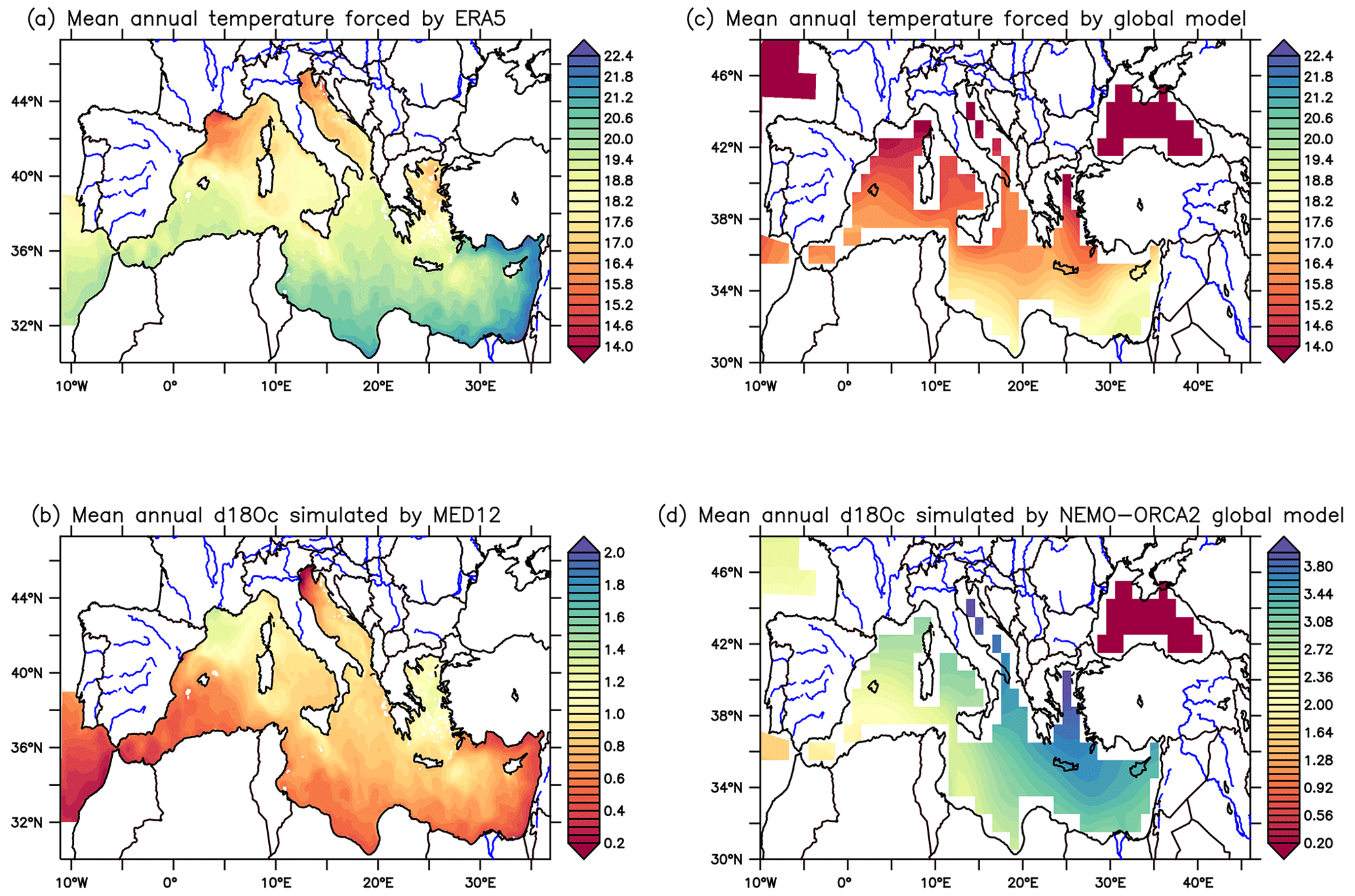
Figure B1 Comparison of the δ¹⁸O_c calculated with high-resolution simulated temperature (a, b) to that derived from a global model using temperature data from LMDZ-iso (c, d).

Appendix C: Assessing the impact of changing the resolution of atmospheric and oceanic models

Sensitivity tests were conducted on the results by altering the horizontal resolution of LMDZ-iso from R96 to R144. A significant correlation was obtained: r² values are 0.66 and 0.68 for the whole basin with LMDZ-iso “R96” and “R144”, respectively. This shows that the δ¹⁸O_w distribution is globally well simulated by the model. However, neither LMDZ-iso R96 nor R144 reproduces the highest values of δ¹⁸O_w observed in the Mediterranean Sea (up to 2.4 ‰ as measured by Gat et al., 1996). Hence, the results of the model are very close between these two horizontal resolutions (R96 and R144) of the LMDZ-iso atmospheric model (Fig. C1), so there may be a certain threshold of spatial resolution below which the simulation is improved by a finer resolution. Vadsaria et al. (2020) demonstrated that high resolution (30 km of the atmospheric model) is critical to accurately capture the synoptic variability needed to initiate the formation of the intermediate and deep waters of the Mediterranean thermohaline circulation (Li et al., 2006). Therefore, we chose to use the R96 resolution, which is the least expensive. Figure C1c displays the δ¹⁸O_w anomaly map between the two simulations R144 and R96. The simulations show a very small difference, ranging between −0.2 and +0.2 ‰. One possible reason for this slight variation is the use of runoff forcing. As described in Sect. 2.2 of the paper, the runoff forcing is based on data from Ludwig et al. (2009) instead of ORCHIDEE. This is because the water flows simulated by ORCHIDEE-iso are unrealistic in the Mediterranean basin. For example, ORCHIDEE-iso significantly overestimates the Nile River discharge. In summary, the change in horizontal resolution between R144 and R96 is not sufficient to generate drastic changes in evaporation and precipitation (as suggested by Vadsaria et al., 2020), and also the fact that the same runoff forcing was used in both the R96 and the R144 simulations explains the small difference between these two simulations despite the change in model resolution. Nonetheless, a dedicated study should be conducted to further elucidate the resolution impact on the tracer distribution.

The model's high resolution presents a unique opportunity to represent a realistic thermohaline circulation in the Mediterranean basin, thus enabling a better understanding of the processes governing water isotopic distribution within this intercontinental basin. Figure C2 illustrates a comparison between the results of the global model (ORCA2, with a 2° horizontal resolution) and the NEMO-MED12 model, both employing the same water isotope modelling approach and driven by the identical atmospheric model, LMDZ-iso (at R96 resolution). The comparison reveals that the global model produces unrealistically high values of δ¹⁸O_w in the Mediterranean Sea, especially in the eastern basin (δ¹⁸O_w>2 ‰, maximum 3.3 ‰), whereas in situ data show maximum values of around 2.1 ‰ (Gat et al., 1996). Overall, high-resolution models can bridge the gap between the coarse resolution of global climate models and the regional to local scales. They can provide a more realistic representation of physical processes and climate feedback compared to global climate models. This is particularly true for the Mediterranean region with complex geology. In particular, atmospheric circulation (high wind gusts in winter) and oceanic circulation (deep convection) are better represented in regional models (Ludwig et al., 2009).

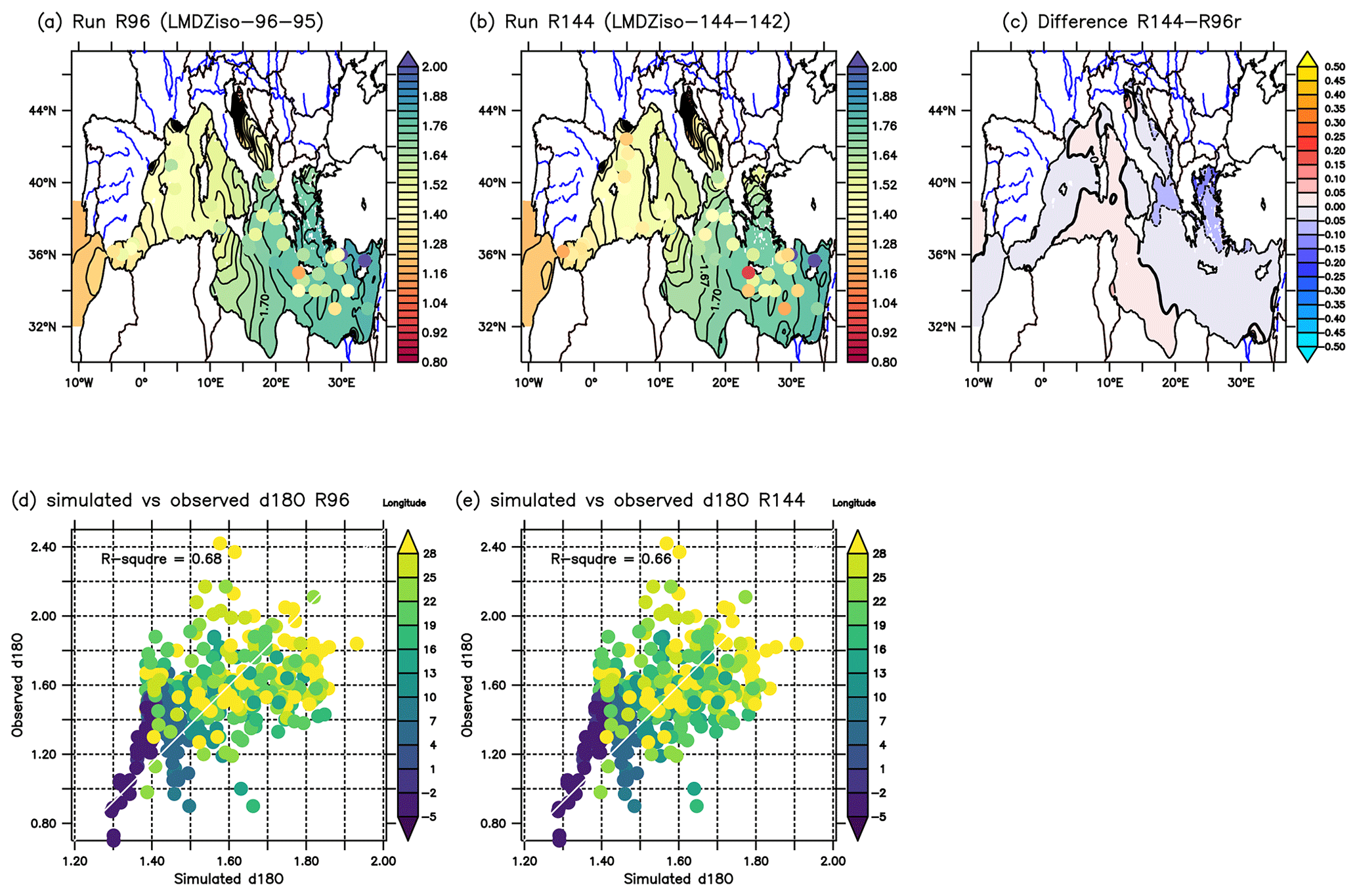
Figure C1 (a) Distribution of δ¹⁸O_w (in ‰) in surface water (at a depth of 50 m) from the R96 simulation. Coloured dots represent in situ observations compiled from Epstein and Mayeda (1953), Stahl and Rinow (1973), Pierre et al. (1986), Gat et al. (1996), and Pierre (1999). Panel (d) presents a multi-scatterplot comparing simulated δ¹⁸O_w (averaged over the last 30 years of the simulation) from the R96 simulation with in situ data from the aforementioned sources across the entire basin. The colour code indicates the longitude of the data in degrees east (° E). Panels (b) and (e) depict the same as panels (a) and (d), respectively, but from the R144 simulation. Panel (c) illustrates the δ¹⁸O_w anomaly map between the R144 and R96 simulations in surface water.

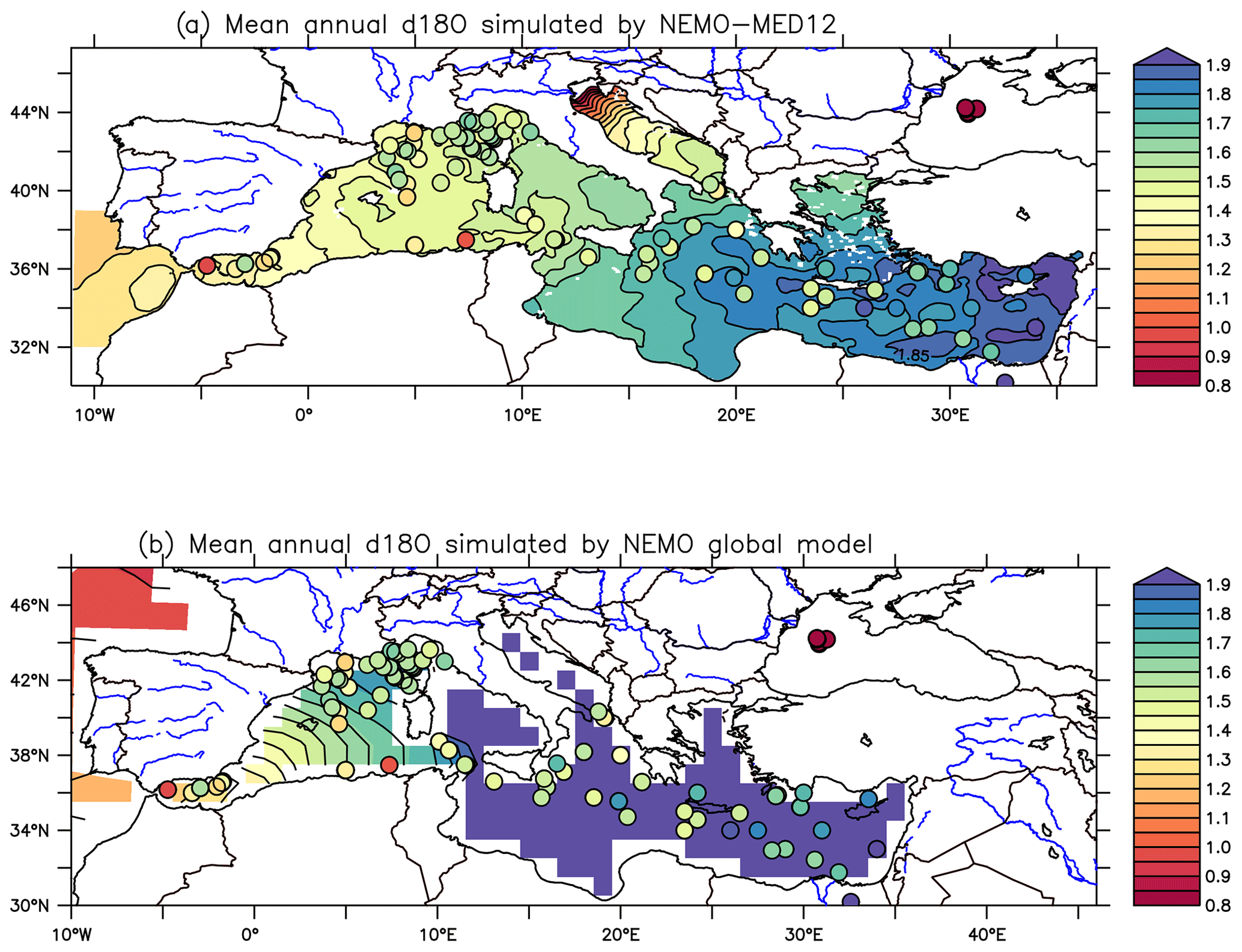
Figure C2 Comparison between the δ¹⁸O_w results of the global model (ORCA2, 2° resolution) and NEMO-MED12 model, using the same water isotope modelling approach and forced by the same atmospheric model, LMDZ-iso (R96).

Appendix D: Pseudo-salinity against standard simulated salinity

The water fluxes from the stand-alone (non-coupled) experiments with LMDZ-iso are not identical to those constraining NEMO-Med12. Hence δ¹⁸O_w or δD_w computed with the water fluxes obtained with LMDZ-iso would not be consistent with the salinity predicted by NEMO-Med12. For this reason, we compute a pseudo-salinity 𝒮_w (Delaygue et al., 2000; Roche et al., 2004). This additional passive tracer does not affect the ocean dynamics. Its sole purpose is to allow a coherent assessment of the relation of the isotopic fields predicted by the model with salinity, since they are computed with the same freshwater forcing.

The evolution equation for 𝒮_w is given by

$$\begin{array}{}\text{(D1)}& \mathit{\rho }K▽{\mathcal{S}}_{\mathrm{w}}=(\mathcal{E}-\mathcal{P}-\mathcal{R}+|\mathcal{I}\left|\right){\mathcal{S}}_{\mathrm{w}}-\left(S_{\mathrm{w}}\mathcal{I}\right).\end{array}$$

Let ℰ, 𝒫, and ℛ represent evaporation, precipitation, and runoff, respectively; 𝒮_w is the salinity of water, and ℐ is the net freshwater flux associated with sea ice formation. With the further assumption that the salinity associated with evaporation, precipitation, and runoff is zero (no effect of freezing/melting on the concentration/dilution of pseudo-salinity in the Mediterranean Sea), the boundary condition for salinity reads

$$\begin{array}{}\text{(D2)}& \mathit{\rho }K▽{\mathcal{S}}_{\mathrm{w}}=(\mathcal{E}-\mathcal{P}-\mathcal{R}){\mathcal{S}}_{\mathrm{w}}.\end{array}$$

The basic understanding of these atmospheric fluxes is that evaporation tends to increase the surface salinity and the ${}^{\mathrm{18}}\mathrm{O}{/}^{\mathrm{16}}\mathrm{O}$ ratio, in contrast to precipitation and runoff.

In Fig. D1, we have plotted the anomaly in salinity − pseudo-salinity to assess the correspondence between pseudo-salinity results and standard modelled salinity. The well-known east–west gradient is effectively captured by recalculated pseudo-salinity, showing very similar values to those of standard salinity. Minor deviations are noticed in the Gulf of Lions and the Algerian Basin, attributed to overlooked meso-activity impacts in the global LMDZ-iso simulation. Overall, the pseudo-salinity globally yields values that are highly comparable to standard simulated salinity.

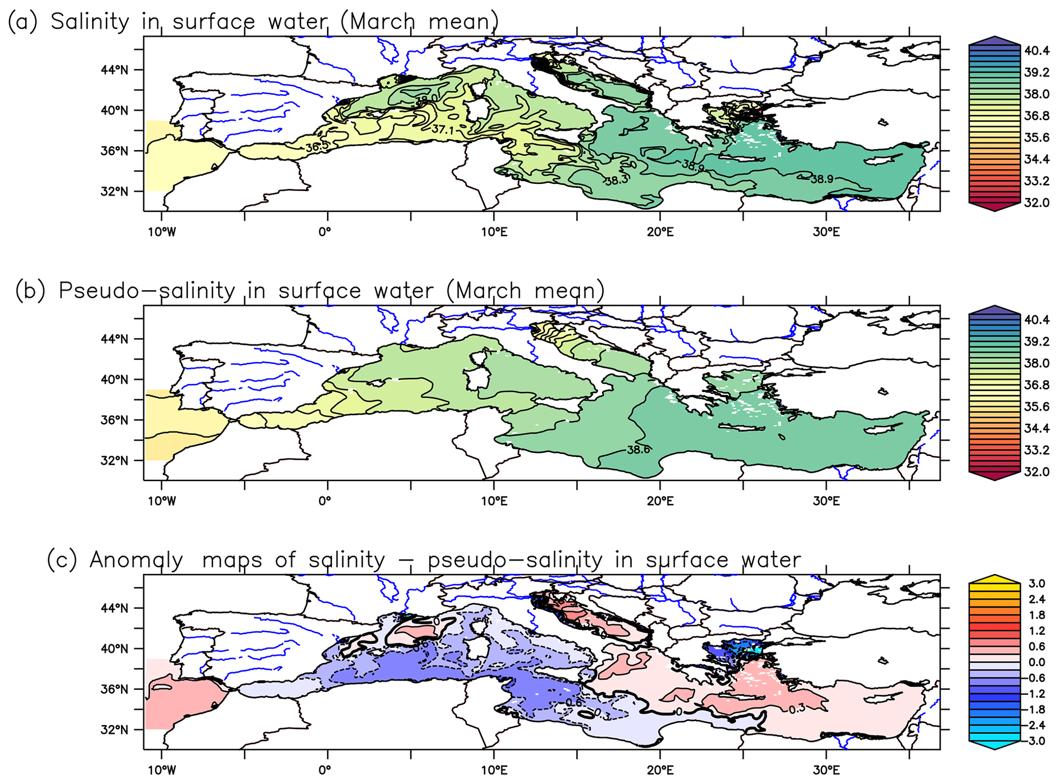
Figure D1 (a) Standard simulated salinity from NEMO-MED12 in the surface model. (b) Pseudo-salinity simulated in the surface water. (c) The anomaly of (a) minus (b).

Appendix E: Sensitivity to isotopic composition input from river runoff

The simulation of surface water isotope fluxes is carried out using the land surface model ORCHIDEE. Isotopes are incorporated into the river discharge of ORCHIDEE-iso, as described by Risi et al. (2016). However, the isotopic version of ORCHIDEE-iso is outdated and cannot be coupled with the current version of LMDZ-iso. A joint project is currently underway to reintroduce water isotopes in the new versions of ORCHIDEE and to couple them with LMDZ-iso. LMDZ-ORCHIDEE numerical experiments already performed by Risi et al. (2010b) provide monthly mean isotopic and freshwater fluxes except for runoff values.

We have conducted sensitivity simulations to assess the impact of computing the isotopic composition of rivers based on the isotopic composition of precipitation (as explained in the paper; see Sect. 2.3). Two new experiments (EXP1 and EXP2) were conducted using output from an earlier version of LMDZ-iso coupled to ORCHIDEE-iso (see Risi et al., 2016) at a lower resolution of 96 × 71.

• EXP1. This employed the approach described in Sect. 2.3 of the paper, where ¹⁸R_river= ¹⁸R_precip × ¹⁸R_runoff.

• EXP2. This integrated the simulated δ¹⁸O of rivers from the older version of LMDZ-iso at 96 × 71 resolution, where ¹⁸R_river = ¹⁸R_riverLMDZiso × ¹⁸R_runoff.

Here, ¹⁸R_precip and ¹⁸R_riverLMDZiso are derived from LMDZ-iso (96 × 71; Risi et al., 2016), while ¹⁸R_runoff is from the interannual dataset of Ludwig et al. (2009) and the RivDIS dataset from Vörösmarty et al. (1996).

The results of these sensitivity simulations are shown in Fig. E1. In EXP1, the model reproduces a reasonable east–west gradient that is similar to our results using a higher version of LMDZ-iso (R96), as shown in Fig. 2a. In EXP2, the addition of the δ¹⁸O of rivers simulated by LMDZ-iso reveals a more enriched isotopic composition (¹⁸O_river) compared to δ¹⁸O_precip. Indeed, evaporation can enrich heavier isotopes in the remaining water, including rivers, which is particularly evident for the Po River, exhibiting a clear positive anomaly of around 0.5 ‰ near the coast and dispersed over the Adriatic Sea. The impact of this and other major rivers (e.g. the Rhône) remains very close to the coast, rapidly dispersed by circulation.

However, the impact of the Nile significantly influences the δ¹⁸O_w signal simulated in EXP2, highlighting a well-known issue in ORCHIDEE-iso concerning the simulation of Nile discharge, where ORCHIDEE-iso tends to largely overestimate the discharge, as depicted in Fig. E1.

Consequently, we opted not to utilise the global version of LMDZ-iso due to the complex hydrology of the Mediterranean region. Instead, we employed a combination of model outputs and in situ data to estimate the runoff amounts entering the Mediterranean Sea. For the isotopic composition, we adopted the same approach as that used by Delaygue et al. (2000).

In conclusion, these sensitivity simulations (EXP1 and EXP2) showed an enrichment of ¹⁸O_river in the rivers due to evaporation, especially for the Po. The influence of the Nile significantly affects the signals, which has prevented the use of this version of LMDZ-iso (R71), and we are unable to couple this old version of ORCHIDEE (outdated) with the current version of LMDZ-iso. Therefore, the approach of Delaygue et al. (2000) was chosen over the data for its reproducibility and usability in paleo-simulations.

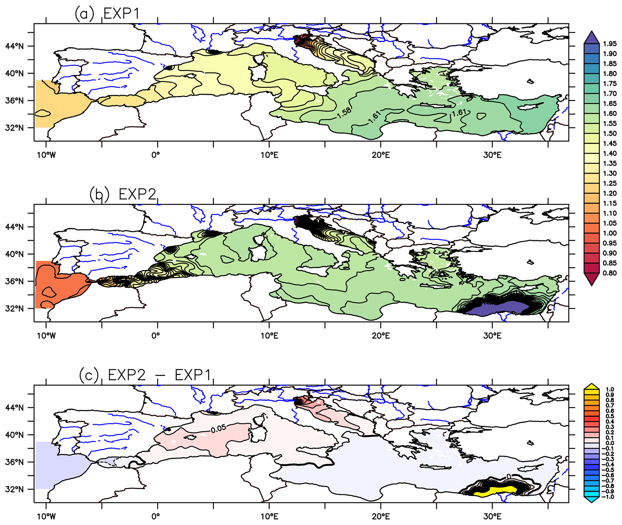
Figure E1 (a) EXP1: we use the same approach as described in our paper; i.e. ¹⁸R_river=¹⁸R_precip × ¹⁸R_runoff. (b) EXP2: we added the ¹⁸O_river simulated by the old version of LMDZ-iso at a lower resolution of 96 × 71; i.e.  ¹⁸R_river=¹⁸R_riverLMDZiso × ¹⁸R_runoff. (c) The difference of EXP2 − EXP1.