the Creative Commons Attribution 4.0 License.
the Creative Commons Attribution 4.0 License.
 | 03 Sep 2024
Exploring the footprint representation of microwave radiance observations in an Arctic limited-area data assimilation system
Stephanie Guedj
Roger Randriamampianina
The microwave radiances are key observations, especially over data-sparse regions, for operational data assimilation in numerical weather prediction (NWP). An often applied simplification is that these observations are used as point measurements; however, the satellite field of view may cover many grid points of high-resolution models. Therefore, we examine a solution in high-resolution data assimilation to better account for the spatial representation of the radiance observations. This solution is based on a footprint operator implemented and tested in the variational assimilation scheme of the AROME-Arctic (Application of Research to Operations at MEsoscale – Arctic) limited-area model. In this paper, the design and technical challenges of the microwave radiance footprint operator are presented. In particular, implementation strategies, the representation of satellite field-of-view ellipses, and the emissivity retrieval inside the footprint area are discussed. Furthermore, the simulated brightness temperatures and the sub-footprint variability are analysed in a case study, indicating particular areas where the use of the footprint operator is expected to provide significant added value. For radiances measured by the Advanced Microwave Sounding Unit-A (AMSU-A) and Microwave Humidity Sounder (MHS) sensors, the standard deviation of the observation minus background (OmB) departures is computed over a short period in order to compare the statistics of the default and the implemented footprint observation operator. For all operationally used AMSU-A and MHS tropospheric channels, it is shown that the standard deviation of OmB departures is reduced when the footprint operator is applied. For AMSU-A radiances, the reduction is around 1 % for high-peaking channels and about 4 % for low-peaking channels. For MHS data, this reduction is somewhere between 1 %–2 % by the footprint observation operator.
- Article
(10306 KB) - Full-text XML
- BibTeX
- EndNote


Satellite radiances are essential components of operational state-of-the-art data assimilation (DA) systems. Microwave sounders and their tropospheric sounding channels are dominant contributors, providing vital atmospheric observations over data-sparse regions like the Arctic (Bormann et al., 2017; Randriamampianina et al., 2019). However, in limited-area models (LAMs), radiance DA is challenging for several reasons. For example, the irregular data sample at the different analysis times is one reason that leads to specific treatment of the variational bias correction (Randriamampianina et al., 2011; Lindskog et al., 2012; Cameron and Bell, 2016; Benáček and Mile, 2019). In most operational numerical weather prediction (NWP) systems, radiance DA was developed and implemented in coarse-resolution models. It makes the high-resolution DA systems suboptimal when the satellite products are used as point measurements and when the representation error is not taken into account. Despite all these challenges, satellite radiances and in particular microwave data have positive impact on analyses and forecasts in LAMs (e.g. Randriamampianina et al., 2019; Lindskog et al., 2021). In general, the use of radiance measurements is more straightforward over open ocean in clear-sky conditions, and the complexity of their assimilation grows with increased sensitivity to the non-ocean surface and over areas affected by precipitation and clouds.
Over sea, the available water emissivity models at microwave frequencies are accurate (e.g. Liu et al., 2011) and have been successfully employed by many operational DA centres. Over land and sea ice, the surface emissivity and skin temperature are more uncertain and depend on various surface parameters. The surface emissivity atlases (e.g. Aires et al., 2011) and dynamic emissivity retrievals (Karbou et al., 2006, 2014; Baordo and Geer, 2016) facilitate the use of surface-sensitive microwave radiances over non-ocean surfaces. The dynamic emissivity method is based on a surface emissivity retrieval from window channel observations and also using background information of the NWP model for both temperature and humidity-sounding channels. This method enabled further extension of the assimilation of surface-sensitive microwave data over land as well as the extension of the use of humidity-sounding channels over sea-ice and snow-covered surfaces (Karbou et al., 2010; Di Tomaso et al., 2013). Another major advancement was achieved by the implementation of the all-sky radiance DA (Bauer et al., 2010; Geer et al., 2014), which significantly increased the number of active radiance observations sensitive to cloud and precipitation. However, these developments still have limitations where stronger sensitivity to land and sea-ice surfaces are present and thus radiance data need to be rejected. At the European Centre for Medium-Range Weather Forecasts (ECMWF), further developments have been initiated to appropriately assimilate radiance data over complex or mixed surfaces, which is called the all-sky all-surface approach (Geer et al., 2022). Recently, a better representation of satellite radiance measurements in DA was studied by Bormann (2017) and Shahabadi et al. (2020) through the implementation of slant-path observation operators.
The above-mentioned radiance DA developments initiated in global models have been gradually implemented in many regional DA systems (e.g. Schwartz et al., 2012; Storto and Randriamampianina, 2010; Lindskog et al., 2021); however, the all-sky assimilation and the use of low-peaking channels still remain the subject of research at many centres. Randriamampianina et al. (2021) showed that radiance observations assimilated in global models have a significant impact on LAM systems through the lateral boundary conditions. In the global model context, Lawrence et al. (2019) showed the great importance of microwave data in the Arctic, where the radiance assimilation is more effective during summer because of complexities related to sea ice and snow cover during other seasons, especially in the winter. In limited-area modelling, Randriamampianina et al. (2021) showed that the impact obtained by the microwave radiance is actually larger in the winter, and it might be explained that in global models a large part of the radiance data need to be rejected and that allows the LAM system to gain a larger impact during winter by microwave radiance data assimilation. This assumption is based on the fact that regional upper air gains the majority of the observation impact through the lateral boundary condition (LBC). So, the higher the quality of the LBC, the lesser the impact of observations through the regional DA. One of our earlier observing system experiment (OSE) studies (Randriamampianina et al., 2021) supports this: use of a low-quality LBC allows for a higher observation impact through regional DA. In high-resolution DA, the satellite field of view (FOV) is not represented by the existing observation operator, which leads to increased representation error. The representation error (Janjić et al., 2017) by definition is an error component that might come from the unresolved scales and processes of the high-resolution observations. However, in high-resolution models, the opposite scale mismatch often occurs when unobserved scales and processes of the NWP model cause the representation error in DA (Marseille and Stoffelen, 2017; Mile et al., 2021). In high-resolution LAMs, the footprint operator aims to reduce the error related to spatial representation error by avoiding the correction of the smallest scales of the model in the DA procedure. The footprint-featured operators have been implemented in different geoscientific applications, e.g. in the regional ice analysis system of Environment Climate Change Canada (Buehner et al., 2013; Carrieres et al., 2017) or in the recently studied scatterometer and Aeolus data assimilation in regional NWP (Mile et al., 2021, 2022). In radiance data assimilation, the importance of the satellite footprint representation has been recognised as well. Kleespies (2009) showed that the aggregation of model surface quantities over the satellite footprint of the microwave radiances might be important when the surface parameters vary substantially. Di et al. (2021) also showed that current IR sounders have typical average sub-footprint brightness temperature variations between 0.8 and 1.5 K over land and a 1 K variation in the 6.25 µm water vapour absorption band, which suggest the importance of the IR footprint representation in DA. Probably for the first time, Duffourg et al. (2010) studied a radiance footprint operator of infrared radiances for a convective-scale DA system over the Mediterranean domain. Recently, Chen et al. (2022) proposed another approach to reduce representation error in microwave radiance data assimilation by applying the so-called remapping technique based on a convolutional neural network.
In this study, we aim to explore the importance of the footprint representation of microwave radiance observations, focusing on an Arctic NWP domain and using the AROME-Arctic mesoscale model (Randriamampianina et al., 2019). Section 2 explains the data and methods of this study, i.e. the microwave radiances and the NWP model configurations. Section 3 describes the challenges of the footprint representation and the implemented footprint operator. In Sect. 4, a case study is analysed in order to assess the importance of the footprint representation by examining the variability in simulated brightness temperatures inside the satellite FOV. Section 5 presents data assimilation diagnostics, and Sect. 6 draws the conclusions and future developments.
2.1 The microwave sounding measurements
The Advanced Microwave Sounding Unit-A (AMSU-A) was designed to measure temperature profiles by a across-track scanning radiometer. The AMSU-A sensor detects radiances in 15 discrete frequencies from 23.8 to 89 GHz, having 11 sounding channels near the oxygen absorption band for temperature sounding and 4 other channels more sensitive to the surface. At each channel frequency, the instrument provides 30 observations from −48 to +48° with respect to the nadir direction. The geometric resolution of a circular instantaneous FOV (IFOV) at nadir has roughly 48 km diameter size, and it is gradually increased towards the edges of the swath to roughly 147 km for across-track and 79 km for along-track resolutions, forming an elliptical IFOV. The Microwave Humidity Sounder (MHS) was designed for tropospheric humidity retrievals by a self-calibrating, across-track scanning, five-channel microwave radiometer. The MHS scans the atmosphere in frequencies from 89 to 190 GHz with three channels dedicated to the strong 183.3 water vapour line and two others called window channels at 89 and 157 GHz. The instrument produces 90 observations of each channel with the approximate nadir resolution of 16 km at a nominal altitude of 833 km. The footprint size increases towards the edges of the swath like in the case for all across-track scanning satellites and reaches 53 km for across-track and roughly 27 km for along-track resolutions. More details about the scanning geometries of the AMSU-A and MHS instruments can be seen in NOAA (2014) and EUMETSAT (2016). These microwave instruments are carried on board EUMETSAT's (European Organisation for the Exploitation of Meteorological Satellites) Metop (Meteorological Operational satellite) and NOAA's (National Oceanic and Atmospheric Administration) satellites. Examples of AMSU-A and MHS FOV footprint ellipses are shown near the edge of the swath (Fig. 1a) and around the nadir (Fig. 1b) position over northern Scandinavia.
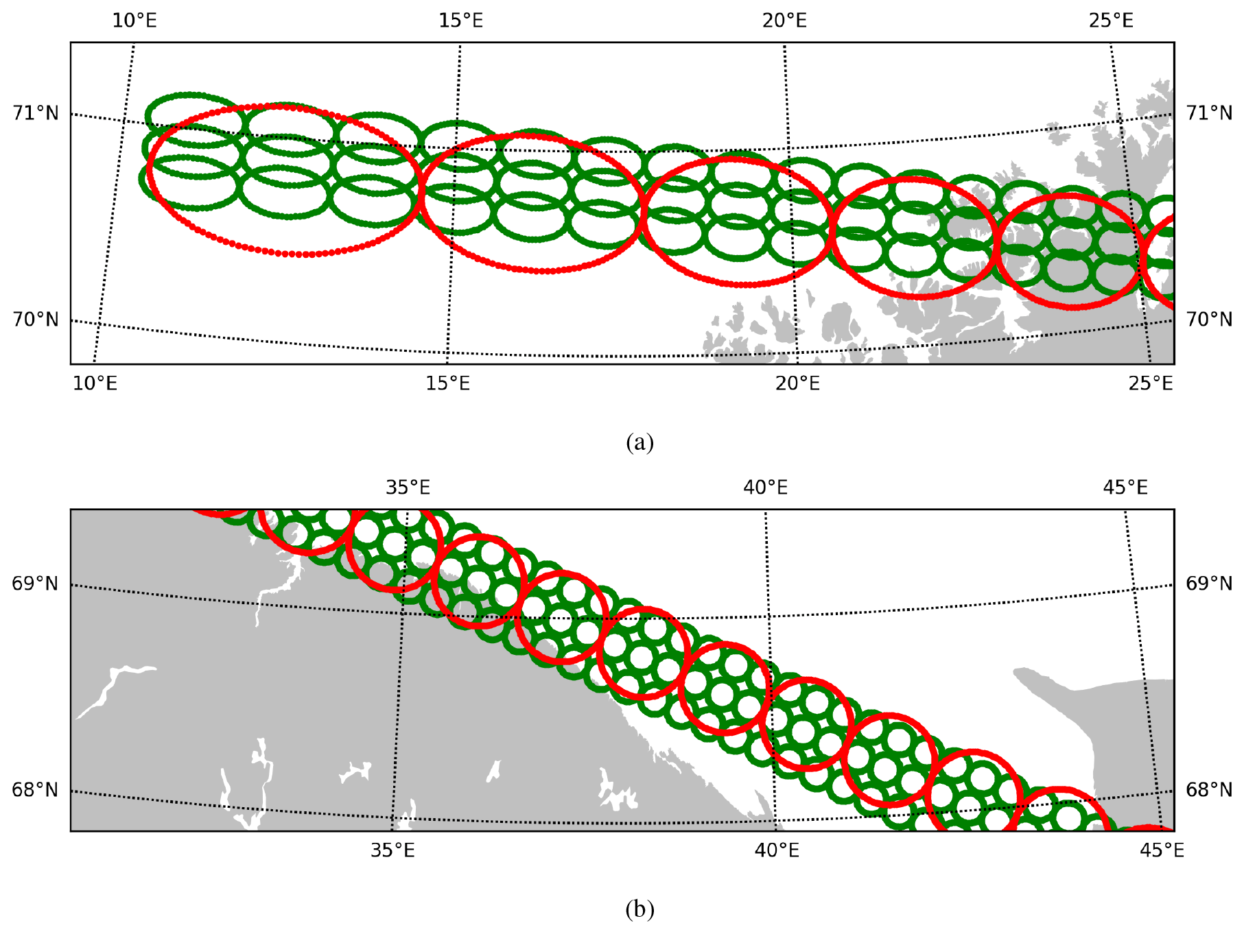
Figure 1The FOV footprint ellipses for AMSU-A (red) and MHS (green) sensors on the Metop-C satellite near the edge of the swath (a) and around nadir (b). Sample taken from a measurement on 20 March 2020, 08:28 UTC.
2.2 AROME-Arctic operational assimilation system
The AROME-Arctic (AA) model (Müller et al., 2017; Randriamampianina et al., 2019) is one of the regional NWP models used at The Norwegian Meteorological Institute (MET Norway). It has been operational since November 2015 and covers parts of the Norwegian, Barents, and Greenland seas; the Svalbard archipelago; and northern Scandinavia. In our study, the model code version 43h2.1 is used in both the reference and the radiance footprint operator implementation runs. The AA model uses 2.5 km horizontal resolution and 65 vertical levels, which is the current operational setup. The AA system assimilates all available conventional and many non-conventional observations from polar-orbiting meteorological satellites. Regarding the use of microwave radiance observations, AA uses data from Metop-B, Metop-C, NOAA-18, and NOAA-19 satellites. In the observation operator of the AA assimilation system, the radiative transfer model RTTOV (version 11.2, Radiative Transfer for TOVS) is incorporated (NWP SAF, 2013). The radiance observations are not assimilated in full resolution due to their correlated observation errors; therefore, satellite data undergo a two-step thinning procedure in which the minimum distance is ensured first, then the thinning to an average distance is done as a second step. The minimum and average thinning distances are 60 and 80 km for AMSU-A and 40 and 80 km for MHS radiances, respectively. The microwave radiances are assimilated operationally in clear-sky conditions using the following channels: 5, 6, 7, 8, and 9 from the AMSU-A and 3, 4, and 5 from the MHS instruments. Near the edge of the satellite swath, the operational system rejects the first and last three and nine IFOVs of AMSU-A and MHS, respectively. The AA assimilation system utilises the three-dimensional variational (3D-Var) scheme (Fischer et al., 2005), with a 3-hourly updated assimilation cycle producing eight analyses per day. The background error covariance matrix was computed considering a dataset for four seasons from the downscaled ECMWF ensemble data assimilation (EDA) runs. In this study, we do not aim to modify the predefined background and observation errors, although the use of the newly developed footprint operator might prefer the recomputation or the tuning of these errors and adjustment of the quality control procedure.
3.1 The choice of the radiance footprint operator
By the default observation operator, radiance data (just like any other observation type) are assimilated as point observations, and a horizontal interpolator (mostly bilinear interpolation using four neighbouring grid points) is employed to generate the model equivalent at the observation location. In order to take into account the satellite footprint, this procedure needs to be replaced or extended. Generally, a footprint operator computes the average of high-resolution model quantities over the footprint of the satellite sensor.
For the implementation of the radiance footprint operator, different strategies and solutions can be considered (see for instance Duffourg et al., 2010). One solution would be to completely replace interpolation with an averaging technique using the model quantities around the observation location, i.e. it does the averaging in model space. Such an implementation would be cost efficient due to the fact that only one piece of averaged model information is needed as input for RTTOV. However, it still requires an extended computational domain or computational halo to access the increased number of grid points (see the example in Mile et al., 2021). Another more expensive and probably more sophisticated implementation might be to apply the averaging in observation space after the interpolation. In this case, several additional operator points around the actual geolocation of the data are needed to construct the instrument footprint. The AA model source code as part of the ARPEGE/IFS (Action de Recherche Petite Echelle Grande Echelle/Integrated Forecasting System) model family has an already existing feature for such developments using the so-called 2D-GOM arrays (Grid-based Observation and Model interpolation). These arrays can store additional model profiles (model-equivalent profiles) for complex observation operators like the slant-path radiance operator (Bormann, 2017) in ECMWF's IFS global model, the radar reflectivity operator in AROME-France (Wattrelot et al., 2013), the slant total delay observation operator (de Haan et al., 2020), or the Aeolus footprint operator (Mile et al., 2022) in HARMONIE-AROME (HIRLAM ALADIN Research on Mesoscale Operational NWP In Europe – convective-scale forecasting system – AROME). Considering the footprint representation in observation space, there can still be different options for where to perform the average in the footprint operator related to the trade-off between complexity and computational cost. One option would be to average the model quantities (over the IFOV) before the actual call of RTTOV, neglecting the non-linear behaviour of the radiative transfer and saving computer resources by executing RTTOV only once. Another, more advanced, solution would be to run RTTOV for all model profiles (inside the IFOV), contributing to the footprint operator independently, and to average them afterwards, taking into account the non-linear effects of RTTOV.
In this study, our aim is to explore the more advanced solution for the microwave radiance footprint operator; therefore, the averaging in observation space after the RTTOV calls has been implemented. The implementation involves many technical challenges which are discussed in the following sections.
3.2 The representation of IFOV and the sampling of the footprint operator points
Both AMSU-A and MHS are across-track scanning instruments with similar scanning geometry properties. The antenna beamwidth of each AMSU-A channel is around 57.6 mrad (milliradians, 3.3°), making a circular IFOV, and the sampling angular interval is roughly 58.18 mrad (3.3333°). The distance between satellite scans is around 52.69 km. Regarding the MHS sensor, the beamwidth of each channel is approximately 19.2 mrad (1.1°), and the sampling angular interval is around 19.39 mrad (1.1111°). The distance between MHS consecutive scans is roughly 17.56 km. The IFOV area for both instruments at nadir forms a perfectly circular footprint with diameters of 48 and 16 km for AMSU-A and MHS, respectively. When the sensor points towards the edge of the scan, the footprint area elongates notably in the across-track direction while only slightly in the along-track direction. The footprint ellipses of such radiance instruments can be described and defined by their minor and major axes relative to the nadir viewing angle of the satellite. The viewing angle of the pixel centre and the vertices of a given IFOV ellipse can be expressed as
where the δstep and ϵ stand for the sampling angular interval (i.e. centre to centre IFOV step angle) and the half of the IFOV width, respectively. p means the pixel number; furthermore, α, αs, and αe stand for the viewing or scanning angle of the pixel centre and the two across-track (i.e. start and end) vertices of the IFOV ellipse, respectively. These α viewing angles can be converted in order to obtain the scanning angle (hereafter γ) on the Earth's surface as the following:
where RE is Earth's radius, and Hsat is the altitude of the satellite at a given geographical location. In Fig. 2, an illustration of across-track scanning field-of-view ellipses and the introduced scanning angles is presented.
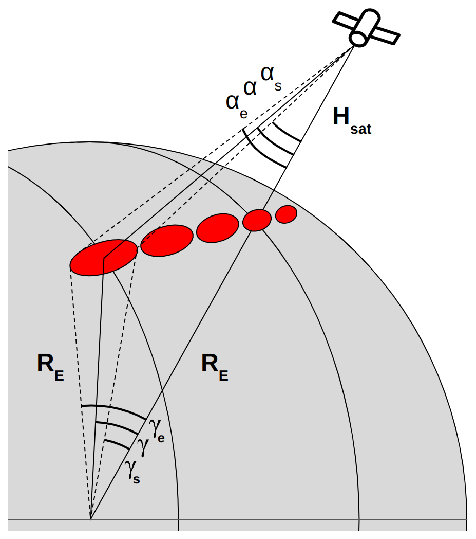
Figure 2Schematic satellite field-of-view ellipses and the scanning angles of the IFOV centre and ellipse vertices for the first IFOV of the swath.
The length of the major axis of an IFOV ellipse on the Earth's surface, therefore, can be expressed as
and the satellite's slant path can also be expressed using the law of sines to compute the minor axis of the IFOV ellipse as follows:
Using dmajor and dminor, the actual size of the IFOV can be calculated and used for the footprint operator. The spatial sampling of the footprint operator points (hereafter FOPs) should reflect the horizontal resolution of the applied NWP model, taking into account the characteristics of the ground-projected IFOV. In our implementation, the FOPs and the geolocations are taken equidistantly along the major and minor axes of an IFOV ellipse; however, this does not result in equal sampling distances within the full satellite scan due to the changing size of the IFOV. Additionally, the same number of FOPs is used in all IFOVs, which is a technical constraint in the current use of 2D-GOM arrays, making the sampling more appropriate for IFOVs with small satellite viewing angles. Nevertheless, in this implementation, the sampling distance on average is close to the model resolution, namely 2.51 and 2.42 km for AMSU-A and MHS, respectively. The FOPs are selected in variable directions around the observation location in order to avoid high-resolution sampling at the centre of the IFOV (see the operator sampling distributions in Figs. 3 and 4). A rotation of the FOPs is also needed to align the IFOV ellipses along the scanning motion or the scanning direction. To this end, the distance of all FOPs from the observation location is computed and rotated by the satellite azimuth as follows:
where Drot consists of the rotated positions of each FOP. and stand for the latitude and longitude locations of the ith point, and φobs and λobs are the actual coordinates of the satellite observation. In Eq. (10), ϕ is the satellite instrument azimuth angle at observation location, and m is the number of FOPs. In order to get the final position of the IFOV, the rotated distances need to be added to the observation geolocation (φobs and λobs), including the variation in distance between meridians with latitude (cos (φobs)). Then IFOV ellipses of the footprint operator are aligned just like the across-track sensors measure them.
In Fig. 3, the AMSU-A FOPs are visualised for a given part of a scanline inside the AA domain. The corresponding observations are shown for MHS FOPs for five neighbouring scanlines (Fig. 4). Note that the pixels near the edges of the swath are also plotted in these figures; however, these pixels are rejected in the operational systems.
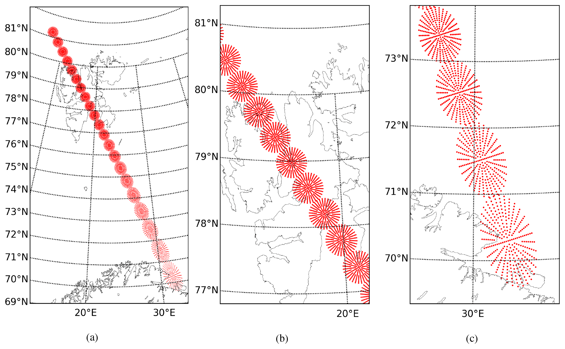
Figure 3The FOPs for AMSU-A FOV ellipses on the Metop-C satellite for one scanline (a), around nadir (b), and near the edge of the swath (c). Sample taken from a measurement on 20 March 2020, 08:28 UTC.
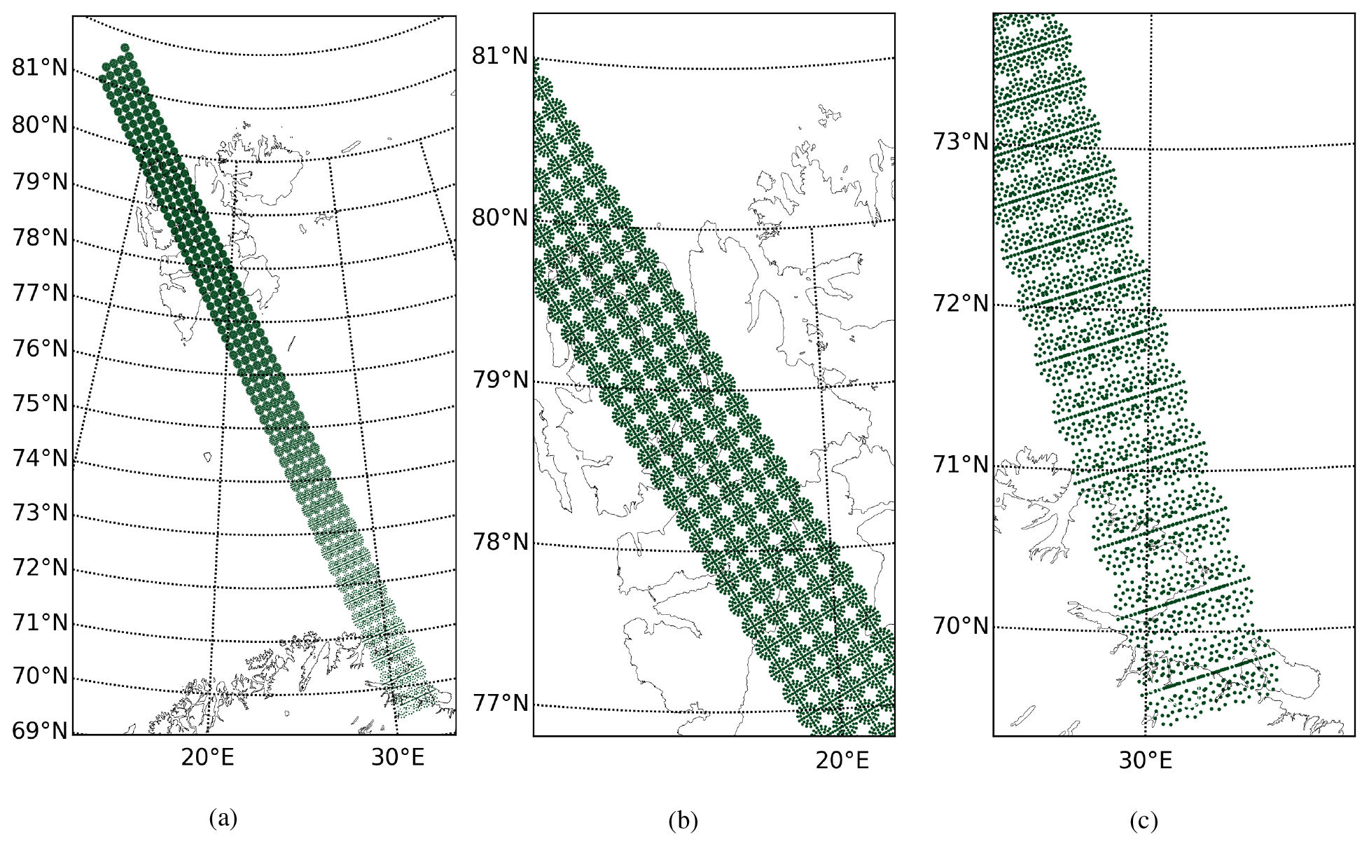
Figure 4The FOPs for MHS FOV ellipses on the Metop-C satellite for five scanlines (a), around nadir (b), and near the edge of the swath (c). Sample taken from a measurement on 20 March 2020, 08:27 UTC.
3.3 The emissivity retrieval in the footprint operator
Emissivity is the ratio of energy emitted from a natural material to that from an ideal blackbody at the same temperature. It varies with the frequency, with the surface type, and also with the observation scan angle. The emissivity is an important component of the radiance data assimilation and difficult to properly determine, especially over non-ocean surfaces. Over open ocean, version 4 of the Fast Microwave Water Emissivity Model (FASTEM-4) is employed (Liu et al., 2011), where the final surface emissivity value of a given radiance dataset is internally computed in the RTTOV model. In the data screening, it means that the open water emissivity is set by a two-step procedure and read/written into the observation database (ODB). Over land, the dynamic emissivity retrieval method (Karbou et al., 2006) is employed. An effective surface emissivity is retrieved from a window channel by reversing the radiative transfer equation. Short-range forecasts of atmospheric profiles and surface information are used as input to RTTOV (see Eq. 11 below). The retrieved emissivity is then allocated to the adjacent sounding channels of the same instrument prior to the assimilation process as the following:
where ϵ(ν,θ) represents the surface emissivity at frequency ν and at observation zenith angle θ. Tb(ν,θ) is the measured brightness temperature by the sensor; furthermore, Ts, , and are the skin temperature and the atmospheric downwelling and upwelling temperatures, respectively. In the AA operational configuration, channel 3 from AMSU-A and channel 1 from MHS are used to retrieve the land surface emissivity. Over sea ice, the surface emissivity is reversed at channel 1 as it was retrieved at channel 2 to account for the frequency dependency (Karbou et al., 2014).
In the footprint operator, the final emissivity can be calculated in different ways depending on the choice of the averaging operation (see Sect. 3.1). For example, one option would be to retrieve one emissivity to be representative of the entire footprint or another – the chosen one of this study – is to derive emissivity values independently for each FOP (hereafter ϵi(ν,θ)). In Fig. 5a, the snapshot of the emissivity ϵi(ν,θ) which is retrieved at AMSU-A channel 3 and then allocated to channel 6 is shown near the Svalbard archipelago. Besides, in Fig. 5b, the sea-ice chart created at MET Norway is presented over the same region for comparison. Near the coastal area of Svalbard, it can be seen that certain AMSU-A IFOVs can have two or even three different surface conditions within a single footprint (see the area of Wahlbergøya and Wilhelmøya, Svalbard). The larger retrieved emissivity values (red colour in Fig. 5b) correspond to land and (thin) sea-ice surfaces, while low emissivity values (blue colour) correspond to open water.
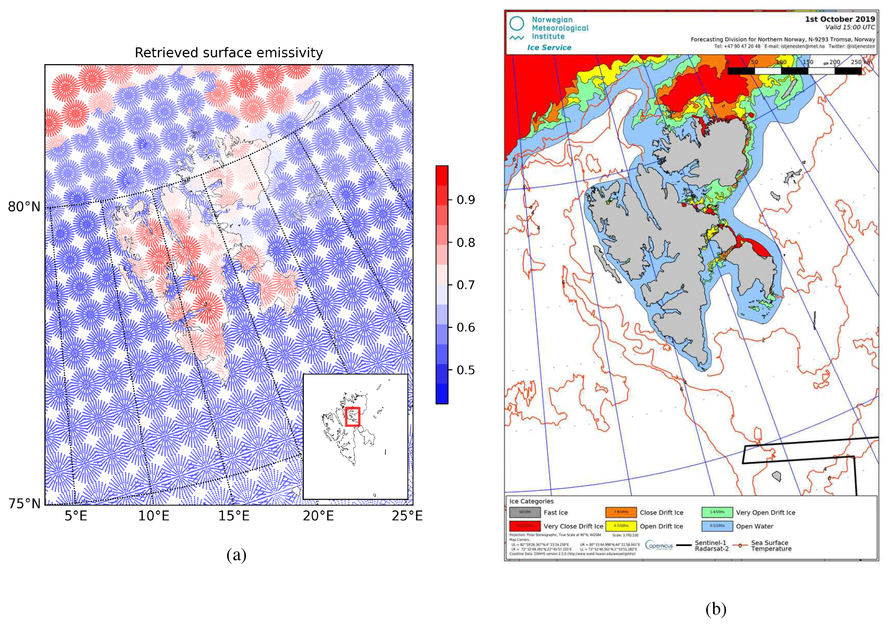
Figure 5The retrieved surface emissivity of AMSU-A observations from the NOAA-18 satellite by the radiance footprint operator with all FOPs (a). In the subplot of Fig. 5a, the area of Wahlbergøya and Wilhelmøya in Svalbard is highlighted. The sea-ice chart of MET Norway's sea-ice service is showing various sea-ice categories (b), namely fast ice (grey), close drift ice (orange), very open drift ice (green), very close drift ice (red), open drift ice (yellow), and open water (blue). The sea surface temperature isolines are indicated by orange lines. Data from 1 October 2019 at 15:00 UTC are used.
One of the main technical challenges for this radiance observation operator is that the default system is interactively using the information stored in the ODB and not designed to handle, for instance, emissivity of the additional FOPs. In our implementation, the AMSU-A footprint operator uses roughly 300 FOPs for a single observation, increasing largely the computational cost of the radiance observation operator. The emissivity values of each FOP (ϵi(ν,θ)) are stored in the extended ODB, providing fast access to the subsequent assimilation tasks. This means that stored emissivity values can be invoked during the minimisation procedure, ensuring the proper use of emissivity for the footprint operator. In Fig. 6a, all ϵi(ν,θ) values are shown for all available AMSU-A channel 6 observations with their corresponding FOPs for the same analysis as is shown in Fig. 5a. In Fig. 6b, the ϵi(ν,θ) values are also shown but only for active data, indicating the result after the data filtering procedure.
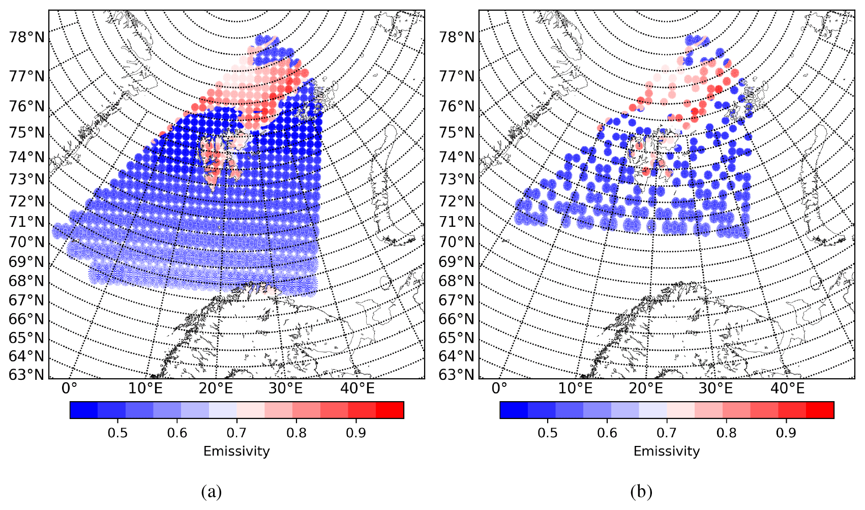
Figure 6Maps of emissivity retrievals using all available AMSU-A channel 6 (a) and active (b) observations from the NOAA-18 satellite, 1 October 2019 at 15:00 UTC, using the radiance footprint operator.
3.4 The footprint observation operator in the variational assimilation scheme
In the variational assimilation framework, the observation operator allows for the computation of the model equivalent of the assimilated observation. In the footprint operator, the model equivalent is calculated for all operator points, and the innovation (hereafter d) is obtained by the use of averaged model equivalents as follows
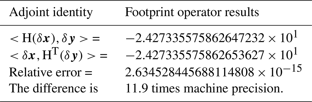
where xb stands for the background state, y is the observation, and ℋ is the observation operator. In the Eq. (13), is the averaged model equivalent to be used in the assimilation, and m is the number of FOPs. This means that the model equivalents are averaged with equal weights in the current implementation of the radiance footprint operator. In the variational assimilation scheme, a linearised observation operator and its conjugate transpose (so-called adjoint operator) are also needed. The footprint operator is built around the default radiance observation operator meaning that the adjoint footprint operator is basically the transpose of the linear averaging operator. In order to verify the correctness of the implemented adjoint operator, the adjoint identity test was produced (see Table 1) and provided comparable results with the default radiance observation operator (not shown).
Table 1The results of the adjoint identity test for the footprint operator using the NOAA-19 AMSU-A satellite radiances in the analysis of 09:00 UTC, 20 March 2020. H is the linear operator and HT is the adjoint footprint operator; is the inner product, and x and y are vectors of the space.
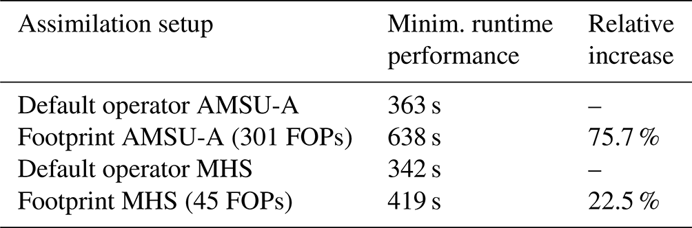
As was already mentioned, the computational cost of the radiance assimilation is significantly increased when the footprint operator is switched on. The main reasons for this are that RTTOV is called multiple times for a single observation and additional operations are needed through the ODB in order to make the proper emissivity retrieval for each FOP. In Table 2, a summary can be seen for the runtime performance of AA minimisation when the default and the footprint observation operator are applied for both AMSU-A and MHS data. The average speed of the minimisation is increased 22.5 % and 75.7 % for MHS and AMSU-A data, respectively, when the introduced footprint operator is employed. It is worth mentioning that these results were obtained with only AMSU-A and MHS sensors and not with the full observing system. Furthermore, it suggests that the optimisation is essential before any real-time applications.
Table 2The mean runtime performance of AA minimisation (Minim.) in seconds using the default operator and the radiance footprint operator with only AMSU-A and MHS data. Additionally, the relative increase in the runtime performance is indicated for the footprint operators. The average runtime performance was determined for the period between 1 and 31 January 2021.
We investigate the simulation of model-equivalent brightness temperatures generated by the radiance footprint operator independent of its use during the assimilation. The radiance footprint operator is efficient when the variability in model fields is considerably large over the footprint area. In order to exhibit the variability in model fields, a case study with developing a polar low (PL) inside the AA domain was investigated. In the morning hours (around 09:00 UTC) of 20 March 2020, the developing PL was moving towards the Lofoten archipelago (see Fig. 7a), causing severe weather events. At this time of the year, the sea-ice extent is substantial inside the AA domain (see Fig. 7b showing the Fram Strait and the Svalbard area), meaning that the chosen case study involved diverse meteorological and surface conditions for studying the radiance footprint operator and the corresponding simulated data.
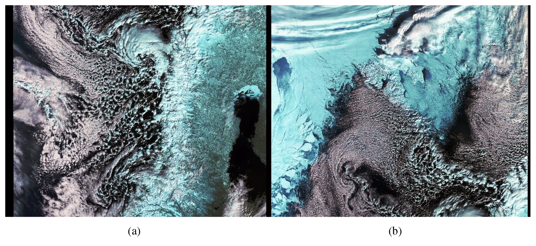
Figure 7Sentinel-3B satellite image captured on 20 March 2020 at 10:16 UTC over the coast of Norway showing a PL (a) and Sentinel-3A satellite image taken on 20 March 2020 at 10:52 UTC over Svalbard showing the sea-ice edge near the Fram Strait and the south of Svalbard (b). Copernicus Sentinel data 2020, processed by the European Space Agency.
The variability in model fields is explored for the available AMSU-A and MHS data inside the AA domain. We compute the variability over the simulated brightness temperatures of the radiance footprint operator (using the FOPs), i.e. the standard deviation of for each satellite IFOV. In Fig. 8a, b, and c, the variability inside each AMSU-A footprint is shown for data from channels 1, 5, and 7, respectively. The colour scales in Fig. 8a, b, and c are different, and this allows us to show only those IFOVs where the standard deviation is the highest. It can be seen in Fig. 8a that the sub-footprint variability likely corresponds to the variable surface conditions in the case of radiance data from AMSU-A channel 1 (23.8 GHz window channel). In Fig. 8d, the retrieved dynamical emissivity is shown, indicating that the highest variability is over the sea-ice edge and the coastal area in northern parts of Scandinavia. In addition to the retrieval done at channel 3 (which is allocated to sounding channels and also being closer in terms of frequency), the emissivity has been retrieved at AMSU-A channel 1. The high variability in the observation equivalent is associated with the impact of mixed surfaces inside the IFOV (see also the area of Jan Mayen island and the corresponding two IFOVs). High-peaking channels of AMSU-A are less or not sensitive to the surface; therefore, sub-footprint variability is not related to mixed-surface conditions. In Fig. 8c, the variability in model equivalents of AMSU-A radiances considering the 54.94 GHz channel (called channel 7) is plotted, and the highest variability is obtained close to the edge of the satellite scan. This might be explained by the fact that IFOV sizes are larger near the edges of the swath, and the corresponding resolution gap is also larger between the model and the observation. In Fig. 8e, the temperature field of the model background is shown, suggesting that there's small or no correspondence between the temperature gradient and the higher sub-footprint variability (Fig. 8c). In Fig. 8b, the variability in model equivalents for AMSU-A channel 5 (53.59 ± 0.115 GHz) can be seen, indicating a combined variability of two sensitivities, namely the surface and atmospheric sensitivities.
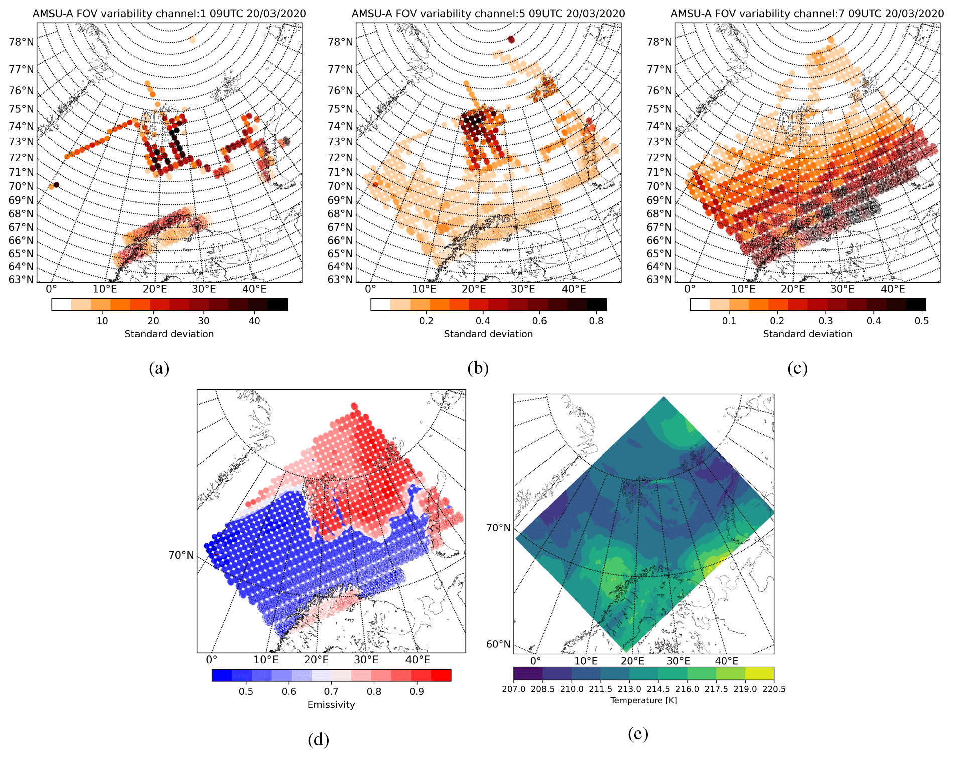
Figure 8The variability in the simulated brightness temperatures inside the footprint of AMSU-A window channel 1 (a), channel 5 (b), and high-peaking channel 7 (c) from the NOAA-19 satellite on 20 March 2020 at 09:00 UTC. The retrieved dynamic emissivity of AMSU-A channel 1 (d) from the NOAA-19 satellite using the radiance footprint operator and showing all emissivity values ϵi(ν,θ) of the FOPs. The AA temperature field (e) at level 15 (around 9 km altitude), valid on 20 March 2020 at 09:00 UTC.
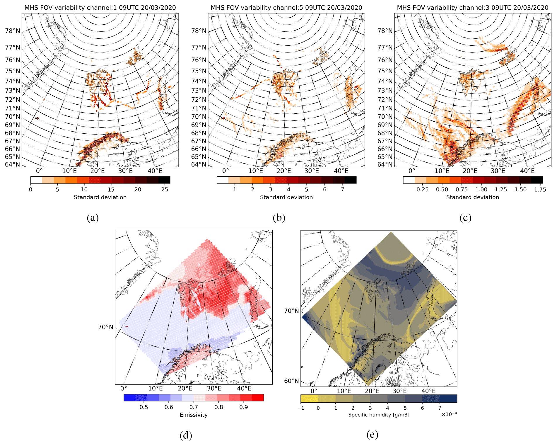
Figure 9The variability in the simulated brightness temperatures inside the footprint of MHS window channel 1 (a), channel 5 (b), and channel 3 (c) from the NOAA-19 satellite on 20 March 2020 at 09:00 UTC. The retrieved dynamic emissivity of MHS channel 1 (d) from the NOAA-19 satellite using the radiance footprint operator and AA specific humidity field (e) at level 30 (around 3.6 km altitude), valid on 20 March 2020 at 09:00 UTC.
In Fig. 9a, b, and c the variability in model-equivalent brightness temperatures is shown for channels 1, 5, and 3 of MHS radiances, respectively. The colour scales are not the same in these figures, indicating only the highest variability and the corresponding footprint. For window channel 1 of MHS (89.0 GHz frequency), similarly to the AMSU-A window channel 1, the standard deviation is the highest over mixed surface, i.e. near the sea-ice edge and around coastal areas (Fig. 9a). Mixed-surface scenes are also visible in Fig. 9d, showing all retrieved emissivity values (ϵi(ν,θ)) of the FOPs for MHS channel 1. In Fig. 9b, the variability map for MHS channel 5 is shown. For this channel, the surface sensitivity and related sub-footprint variability are generally smaller (see standard deviations). This figure reflects a kind of mixture of surface and atmospheric sensitivity through the sub-footprint variability for MHS channel 5 data. For the humidity sensitive channel (see Fig. 9c), the highest variability is obtained over different locations and open ocean areas, suggesting the correspondence with atmospheric humidity conditions independently from the surface. In Fig. 9e, the AA specific humidity field is shown around the same level where the MHS channel 3 is the most sensitive. Basically, the high variability over the MHS IFOVs in Fig. 9b corresponds to the large variability and gradient in the humidity field (see Fig. 9d). It is worth highlighting that the PL area near the Lofoten archipelago has typically larger sub-footprint variability, indicating small-scale variability near the centre of the PL (a closer look at this area is seen in Fig. 10). In this situation, the use of the radiance footprint operator can be particularly important, although this might require the all-sky framework for MHS radiance assimilation as well.
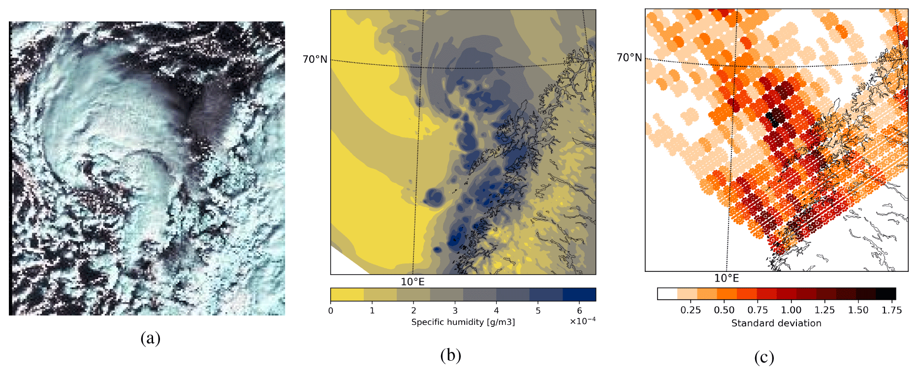
Figure 10Sentinel-3A satellite image captured on 20 March 2020 at 09:14 UTC showing the PL near the Lofoten archipelago (a). Copernicus Sentinel data 2020, processed by the European Space Agency. The AA specific humidity field at level 30 (around 3.6 km altitude) is shown over the Lofoten archipelago (b) on 20 March 2020 at 09:00 UTC. The variability in the simulated brightness temperatures inside the footprint of MHS channel 3 from the NOAA-19 satellite on 20 March 2020 at 09:00 UTC (area over the Lofoten archipelago) (c).
In this section, observation minus background (OmB) departures are examined comparing the statistics of the default and the footprint observation operators for AMSU-A and MHS radiances. The diagnostics are assessed over a 1-month and a 2-month period for AMSU-A and MHS, respectively, excluding short spin-up intervals. For MHS radiances, a longer diagnostic period was necessary to collect enough data inside the AA domain (i.e. amount of data per the scanning position between 1000 and 4000). The radiance observations from Metop-B, Metop-C, NOAA-18, and NOAA-19 satellites are used with accepted pixels near the edges of the swath in the AA assimilation runs. Apart from the applied observation operators, the default assimilation settings, namely the predefined observation and background errors, thinning distances, and the quality control procedure were the same in both assimilation experiments. In Fig. 11a, the standard deviation of OmB departures is plotted using all operationally utilised clear-sky AMSU-A data during the studied period. It can be seen that the use of the radiance footprint operator provides small but consistent reduction in the standard deviation of OmB departures. The same can be concluded from the standard deviation of MHS departures, which is plotted in Fig. 11b.
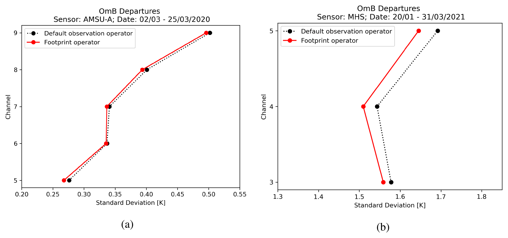
Figure 11The standard deviation of OmB for AMSU-A channels (a) and the standard deviation of OmB for MHS channels (b). The dashed black lines show the statistics of the default radiance observation operator, and the red solid lines are the results of the radiance footprint operator. The statistics were accumulated during the period between 2 and 25 March 2020 for AMSU-A data and the period between 20 January and 31 March 2021 for MHS departures.
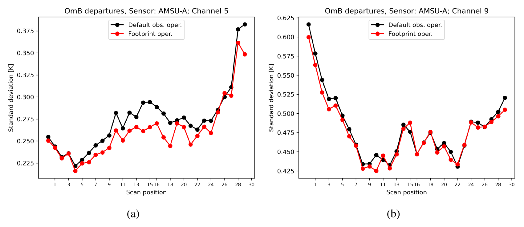
Figure 12The standard deviation of OmB using data of AMSU-A channel 5 (a) and channel 9 (b) as a function of satellite scanning position. The black line stands for the default operator, and the red line is for the footprint operator. The statistics were computed for the period between 2 and 25 March 2020.
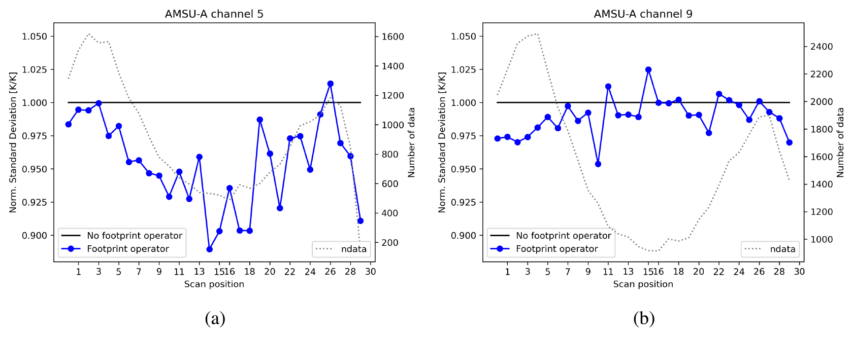
Figure 13The standard deviation of OmB departures from the footprint operator normalised by the statistics from the default operator (blue line) for AMSU-A channel 5 (a) and channel 9 (b) as a function of satellite scanning position. The number of observation minus background differences are also shown with a dashed grey line. The statistics were computed for the period between 2 and 25 March 2020.
In Fig. 12a and b, the standard deviation of OmB departures for AMSU-A channels 5 and 9 are shown as a function of satellite scanning positions. By the use of the radiance footprint operator, the reduction in OmB statistics for channels 5 and 9 is apparent near the edges of the swath and also for smaller zenith angles. It means that taking into account the satellite footprint might help to reduce the difference between observations and model equivalents in the full swath. The reduction is slightly larger near the edges for high-peaking channels which might be explained by the larger representation error for the outermost scan positions. In Fig. 13a and b, the normalised standard deviation of OmB for AMSU-A channels 5 and 9 are shown. For the low-peaking channel, it can be seen that the reduction is considerable for pixels close to the centre of the swath. Additionally, the number of OmB departures are plotted in these figures, showing that the thinning procedure filters more observations at nadir (higher data density) compared to observations near the edges of the swath.
Concerning MHS radiances, the standard deviation of OmB departures for MHS channels 4 and 5 are shown as a function of 90 scanning positions (see Fig. 14a and b). When the MHS footprint operator is applied, the reduction in OmB statistics is noticeable for most of the pixels in the full satellite swath. For this sensor, a longer period was necessary to run in order to gain a larger statistical sample. In Fig. 15a and b, the normalised standard deviations of OmB for MHS channels 4 and 5 are also shown, and it can be seen that the reduction is perceptible for most of the MHS scan positions. Similarly to AMSU-A in Fig. 13a and b, the number of OmB departures are also plotted in these figures.
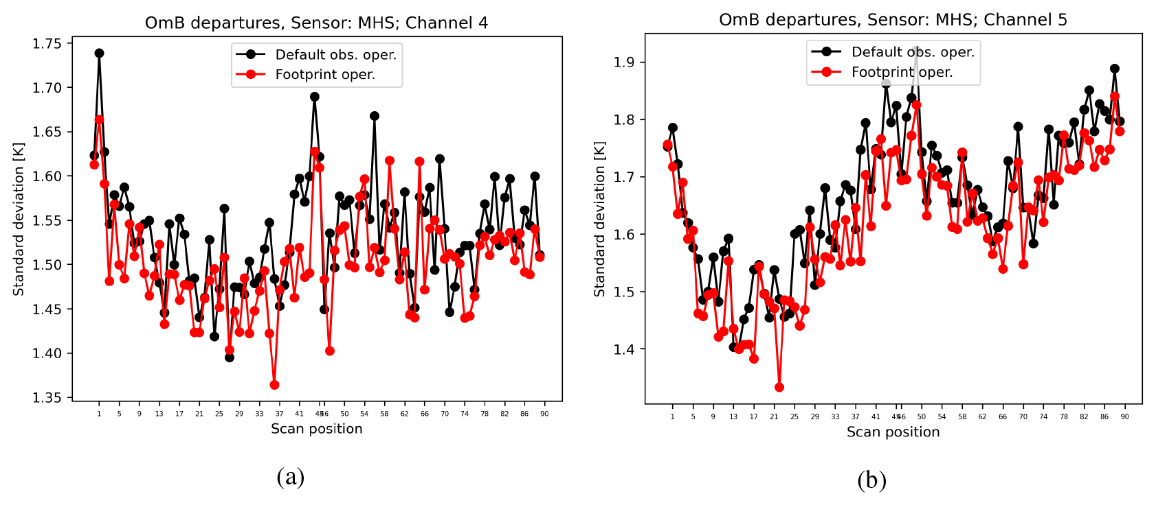
Figure 14The standard deviation of observation minus AA forecasts of MHS channel 4 (a) and channel 5 (b) as a function of satellite scanning position. The black line stands for the default operator, and the red line is for the footprint operator. The statistics were computed for the period between 20 January and 31 March 2021.
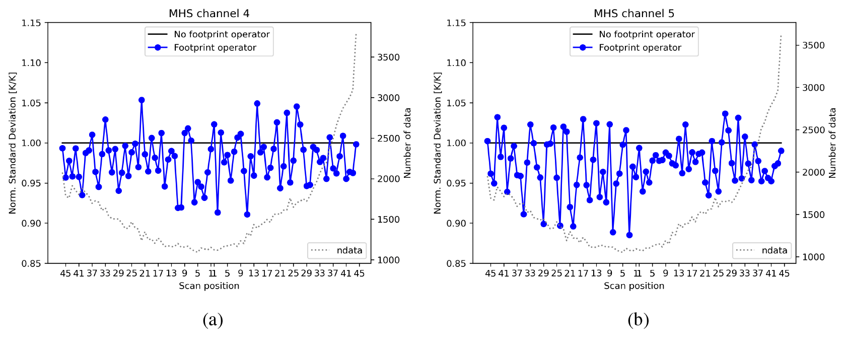
Figure 15The standard deviation of OmB departures from the footprint operator normalised by the statistics from the default operator (blue line) for MHS channel 4 (a) and channel 5 (b) as a function of satellite scanning position. The number of observation minus background differences are also shown with a dashed grey line. The statistics were computed for the period between 20 January and 31 March 2021.
The footprint representation of microwave radiance observations was explored in the mesoscale AA data assimilation system. The resolution gap between the data and the NWP model is apparent, especially for AMSU-A radiances near the edges of the satellite scan. The use of the footprint operator helps to make the data assimilation system more optimal and to avoid constraining unobserved scales and processes in the mesoscale analysis. The implementation of the footprint operator can follow different strategies. In this paper, the averaging operation after the RTTOV simulations was explored, making the implementation computationally more expensive and more appropriate in the non-linear radiance observation operator. Such an implementation in the AROME variational assimilation system involves technical challenges and increased computational costs. For instance, the storage and the proper utilisation of retrieved dynamic emissivity values are challenging tasks in the minimisation procedure for all footprint operator points independently. Beyond the technical implementation, the potential benefit of the radiance footprint operator was investigated in a particular case study, exploring the sub-footprint variability of the simulated data. The added value of the radiance footprint operator is expected to be negligible over areas of homogeneous meteorological conditions, and its use is more important where the variability in model fields is considerably larger. In this case study, we demonstrated that the variability is higher near the edges of the swath (large footprint size) for a high-peaking AMSU-A channel, and the high variability also corresponds to particular weather phenomena like a PL in the case of simulated MHS brightness temperatures. In addition, it is important to further investigate the source or element of sub-footprint inhomogeneity and to quantify their contributions in the representation error. This aspect was identified and discussed by Duncan et al. (2019) using AMSR2 (Advanced Microwave Scanning Radiometer 2), noting that sub-FOV inhomogeneity can be quite important for the lowest frequencies. Furthermore, it will be a major challenge with the use of future instruments like Copernicus Imaging Microwave Radiometer (CIMR) in a high-resolution limited-area modelling framework. Finally, departure-based statistics were investigated for AMSU-A and MHS radiances, showing small but consistent reductions in the standard deviation of OmB. For AMSU-A, the maximum reduction that was obtained for low-peaking channel 5 was around 4 %, and for MHS the reduction is around 1 %–2 %.
Regarding future outlook, the implemented radiance footprint operator can be further developed. For example, the footprint representation helps to take into account heterogeneous conditions inside the IFOV area and to make a better quality control for the radiance observations. Additionally, it might help to better assimilate radiances in the all-sky framework, e.g. to better describe cloud and rain inside the footprint area. The radiance footprint operator might also help to start using satellite observations that are sensitive to the surface, i.e. assimilating radiance over all-surface conditions. The implemented radiance footprint operator uses interpolated FOPs and corresponding vertical profiles, neglecting that the instrument has a slanted path through the atmosphere. Therefore, the combination of the slant-path and the footprint operator can be considered as a future development, improving even further the use of radiance data near the edges of the swath. Furthermore, the introduced footprint operator assumes equal contributions from each FOP and, therefore, applies a boxcar averaging function. However, this might be oversimplified for radiance measurements where the radiance signal strength does not show a uniform distribution, and the satellite footprint is basically defined by the half-power beamwidth. This means that half of the energy where the power is below 3 dB comes from areas (part of the main and side lobes) outside the footprint. In the future development of the radiance footprint operator, the signal strength and the effective field of view need to be considered as well. Furthermore, the representation of the radiance antenna pattern is relevant, and different sampling methods and/or a weighted averaging of FOPs are proposed to be incorporated into the footprint operator. Beyond the improved representation of the radiance footprint, the optimisation is also important for the cost-efficient application. The trade-off between accuracy and cost efficiency is particularly important for future operational use.
The AROME-Arctic assimilation scheme, the implemented footprint operator, and HARMONIE-AROME codes, along with all their related intellectual property rights, are owned by the members of the ACCORD (A Consortium for COnvective-scale modelling Research and Development) consortium. This agreement allows each member of the consortium to license the shared ACCORD codes to academic institutions of their home country for non-commercial research. Access to the codes of the ACCORD system can be obtained by contacting one of the member institutes, which can be done by submitting a request via the “Contact” link at the bottom of the ACCORD website (http://www.umr-cnrm.fr/accord/, last access: 22 August 2024); access will be subject to signing a standardised ACCORD license agreement. The observation dataset (including the departure-based statistics) has been packed and is available for download at Zenodo (https://doi.org/10.5281/zenodo.10851015, Mile, 2024).
MM and RR designed the footprint observation operator, and MM developed the model code. SG instructed the implementation of dynamical emissivity retrieval in the footprint operator. MM designed the experiments and carried them out. MM prepared the manuscript with contributions from all co-authors.
The contact author has declared that none of the authors has any competing interests.
Publisher’s note: Copernicus Publications remains neutral with regard to jurisdictional claims made in the text, published maps, institutional affiliations, or any other geographical representation in this paper. While Copernicus Publications makes every effort to include appropriate place names, the final responsibility lies with the authors.
First of all, the authors are grateful to Pascal Brunel for the guidance of the radiance footprint calculations. Additionally, we are grateful to the ECMWF and Météo-France colleagues for making the basis for the 2D-GOM arrays. The authors kindly acknowledge the support of the Research Council of Norway through the Arctic weather prediction project called ALERTNESS and the support of the high-performance computing facility at ECMWF, where resources were provided via a special project called spnomile.
This research has been supported by the Norges Forskningsråd (grant no. 280573).
This paper was edited by Yuefei Zeng and reviewed by two anonymous referees.
Aires, F., Prigent, C., Bernardo, F., Jiménez, C., Saunders, R., and Brunel, P.: A tool to estimate land-surface emissivities at microwave frequencies (TELSEM) for use in numerical weather prediction, Q. J. Roy. Meteor. Soc., 137, 690–699, https://doi.org/10.1002/qj.803, 2011. a
Baordo, F. and Geer, A. J.: Assimilation of SSMIS humidity-sounding channels in all-sky conditions over land using a dynamic emissivity retrieval, Q. J. Roy. Meteor. Soc., 142, 2854–2866, https://doi.org/10.1002/qj.2873, 2016. a
Bauer, P., Geer, A. J., Lopez, P., and Salmond, D.: Direct 4D-Var assimilation of all-sky radiances: Part I. Implementation, Q. J. Roy. Meteor. Soc., 136, 1868–1885, https://doi.org/10.1002/qj.659, 2010. a
Benáček, P. and Mile, M.: Satellite Bias Correction in the Regional Model ALADIN/CZ: Comparison of Different VarBC Approaches, Mon. Weather Rev. 147, 3223–3239, https://doi.org/10.1175/MWR-D-18-0359.1, 2019. a
Bormann, N.: Slant path radiative transfer for the assimilation of sounder radiances, Tellus A, 69, 1272779, https://doi.org/10.1080/16000870.2016.1272779, 2017. a, b
Bormann, N., Lupu, C., Geer, A., Lawrence, H., Weston, P., and English, S.: Assessment of the forecast impact of surface-sensitive microwave radiances over land and sea-ice, Tech. Memo. 804, ECMWF, Reading, UK, https://doi.org/10.21957/qyh34roht, 2017. a
Buehner, M., Caya, A., Pogson, L., Carrieres, T., and Pestieau, P.: A New Environment Canada Regional Ice Analysis System, Atmos. Ocean, 51, 18–34, https://doi.org/10.1080/07055900.2012.747171, 2013. a
Cameron, J. and Bell, W.: The testing and planned implementation of variational bias correction (VarBC) at the Met Office, https://cimss.ssec.wisc.edu/itwg/itsc/itsc20/papers/11_01_cameron_paper.pdf (last access: 5 June 2022), 2016. a
Carrieres, T., Buehner, M., Lemieux, J. F., and Pedersen, L.: Sea Ice Analysis and Forecasting Towards an Increased Reliance on Automated Prediction Systems, Cambridge University Press, Cambridge, UK., https://doi.org/10.1017/9781108277600 2017. a
Chen, K., Fan, X., Han, W., and Xiao, H.: A Remapping Technique of FY-3D MWRI Based on a Convolutional Neural Network for the Reduction of Representativeness Error, IEEE T. Geosci. Remote, 60, 5302511, https://doi.org/10.1109/TGRS.2021.3138395, 2022. a
de Haan, S., Pottiaux, E., Sánchez-Arriola, J., Bender, M., Berckmans, J., Brenot, H., Bruyninx, C., De Cruz, L., Dick, G., Dymarska, N., Eben, K., Guerova, G., Jones, J., Krč, P., Lindskog, M., Mile, M., Möller, G., Penov, N., Resler, J., Rohm, W., Slavchev, M., Stoev, K., Stoycheva, A., Trzcina, E., and Zus, F.: Use of GNSS Tropospheric Products for High-Resolution, Rapid-Update NWP and Severe Weather Forecasting (Working Group 2), Advanced GNSS Tropospheric Products for Monitoring Severe Weather Events and Climate, 203–265, https://doi.org/10.1007/978-3-030-13901-8_4, 2020. a
Di, D., Li, J., Li, Z., Li, J., Schmit, T. J., and Menzel, W. P.: Can current hyperspectral infrared sounders capture the small scale atmospheric water vapor spatial variations?, Geophys. Res. Lett. 48, e2021GL095825, https://doi.org/10.1029/2021GL095825, 2021. a
Di Tomaso, E., Bormann, N., and English, S. J.: Assimilation of ATOVS radiances at ECMWF: third year EUMETSAT fellowship report, EUMETSAT/ECMWF Fellowship Programme Research Report, No. 29, https://www.ecmwf.int/node/9051 (last access: 22 August 2024), 2013. a
Duffourg, F., Ducrocq, V., Fourrié, N., Jaubert, G., and Guidard, V.: Simulation of satellite infrared radiances for convective‐scale data assimilation over the Mediterranean, J. Geophys. Res. 115, D15107, https://doi.org/10.1029/2009JD012936 2010. a, b
Duncan, D. I., Eriksson, P., and Pfreundschuh, S.: An experimental 2D-Var retrieval using AMSR2, Atmos. Meas. Tech., 12, 6341–6359, https://doi.org/10.5194/amt-12-6341-2019, 2019. a
EUMETSAT: ATOVS Level 1b Product Guide, EUMETSAT Technical Report, Doc no.: EUM/OPS-EPS/MAN/04/0030, https://www-cdn.eumetsat.int/files/2020-04/pdf_atovsl1b_pg.pdf (last access: 22 August 2024), 2016. a
Fischer, C., Montmerle, T., Berre, L., Auger, L., and Stefanescu, S. E.: An overview of the variational assimilation in the ALADIN/France numerical weather-prediction system, Q. J. Roy. Meteor. Soc., 131, 3477–3492, 2005. a
Geer, A. J., Baordo, F., Bormann, N., and English, S.: All-sky assimilation of microwave humidity sounders, Tech. Memo. 741, ECMWF, Reading, UK, https://doi.org/10.21957/obosmx154, 2014. a
Geer, A. J., Lonitz, K., Duncan, D. I., and Bormann, N.: Improved surface treatment for all-sky microwave observations, Tech. Memo., 894, ECMWF, Reading, UK, https://www.ecmwf.int/node/20337 (last access: 22 August 2024), 2022. a
Janjić, T., Bormann, N., Bocquet, M., Carton, J. A., Cohn, S. E., Dance, S. L., Losa, S. N., Nichols, N. K., Potthast, R., Waller, J. A., and Weston, P.: On the representation error in data assimilation, Q. J. Roy. Meteor. Soc., 144, 1257–1278, https://doi.org/10.1002/qj.3130, 2017. a
Karbou, F., Gérard É., and Rabier, F.: Microwave land emissivity and skin temperature for AMSU-A and -B assimilation over land, Q. J. Roy. Meteor. Soc., 132, 2333–2355, https://doi.org/10.1256/qj.05.216, 2006. a, b
Karbou, F., Gérard, É., and Rabier, F.: Global 4DVAR Assimilation and Forecast Experiments Using AMSU Observations over Land. Part I: Impacts of Various Land Surface Emissivity Parameterizations, Weather Forecast., 25, 5–19, https://doi.org/10.1175/2009WAF2222243.1, 2010. a
Karbou, F., Rabier, F., and Prigent, C.: The assimilation of observations from the Advanced Microwave Sounding Unit over sea ice in the French global numerical weather prediction system, Mon. Weather Rev., 142, 125–140, 2014. a, b
Kleespies, T. J.: Microwave radiative transfer at the sub-field-of-view resolution, https://itwg.ssec.wisc.edu/wordpress/wp-content/uploads/2023/05/03_04_kleespies_itsc16.pdf (last access: 22 August 2024), 2009. a
Lawrence, H., Bormann, N., Sandu, I., Day, J., Farnan, J., and Bauer, P.: Use and impact of Arctic observations in the ECMWF Numerical Weather Prediction system, Q. J. Roy. Meteor. Soc., 145, 3432–3452, https://doi.org/10.1002/qj.3628, 2019. a
Lindskog, M., Dahlbom, M., Thorsteinsson, S., Dahlgren, P., Randriamampianina, R., and Bojarova, J.: ATOVS processing and usage in the HARMONIE reference system, HIRLAM Newsletter, 59, 33–43, available from the HIRLAM Project, c/o Jeanette Onvlee, KNMI, AE De Bilt, the Netherlands, 2012. a
Lindskog, M., Dybbroe, A., and Randriamampianina, R.: Use of Microwave Radiances from Metop-C and Fengyun-3 C/D Satellites for a Northern European Limited-area Data Assimilation System, Adv. Atm. Sci., 38, 1415–1428, 2021. a, b
Liu, Q., Weng, F., and English, S.: An improved fast microwave water emissivity model, IEEE Trans. Geosci. Remote, 49, 1238–1250, 2011. a, b
Marseille, G.-J. and Stoffelen, A.: Toward Scatterometer Winds Assimilation in the Mesoscale HARMONIE Model, IEEE J. Sel. Top. Appl., 10, 2383–2393, 2017. a
Mile, M., Randriampianina, R., Marseille, G.-J., and Stoffelen, A.: Supermodding – A special footprint operator for mesoscale data assimilation using scatterometer winds, Q. J. Roy. Meteor. Soc., 147, 1382–1402, https://doi.org/10.1002/qj.3979, 2021. a, b, c
Mile, M., Azad, R., and Marseille, G.-J.: Assimilation of Aeolus Rayleigh-clear winds using a footprint operator in AROME-Arctic mesoscale model, Geophys. Res. Lett., 49, e2021GL097615, https://doi.org/10.1029/2021GL097615, 2022. a, b
Mile, M.: Observation Database for Exploring the footprint representation of microwave radiance observations in an Arctic limited-area data assimilation system, Zenodo [data set], https://doi.org/10.5281/zenodo.10851015, 2024. a
Müller, M., Batrak, Y., Kristiansen, J., Køltzow, M., A., Ø., Noer, G. and Korosov, A.: Characteristics of a convective-scale weather forecasting system for the European Arctic, Mon. Weather Rev., 145, 4771–4787, 2017 a
NOAA: KLM User's Guide with NOAA-N, N Prime, and MetOp Supplements, NOAA, User Guide, available from https://www1.ncdc.noaa.gov/pub/data/satellite/publications/podguides/N-15 thru N-19/pdf/0.0 NOAA KLM Users Guide.pdf (last access: 22 August 2024), 2014. a
Randriamampianina, R., Iversen, T., and Storto, A.: Exploring the assimilation of IASI radiances in forecasting polar lows, Q. J. Roy. Meteor. Soc., 137, 1700–1715, https://doi.org/10.1002/qj.838, 2011. a
Randriamampianina, R., Schyberg, H., and Mile, M.: Observing System Experiments with an Arctic Mesoscale Numerical Weather Prediction Model. Remote Sens., 11, 981, https://doi.org/10.3390/rs11080981, 2019. a, b, c, d
Randriamampianina, R., Bormann, N., Køltzow, M. A. Ø., Lawrence, H., Sandu, I., and Wang, Z. Q.: Relative impact of observations on a regional arctic numerical weather prediction system, Q. J. Roy. Meteor. Soc., 147, 2212–2232, https://doi.org/10.1002/qj.4018, 2021. a, b
Randriamampianina, R., Horányi, A., Bölöni, G., and Szépszó, G.,: Historical observation impact assessments for EUMETNET using the ALADIN/HU limited area model, Q. J. Hung. Meteor. Serv., 125, 521–692, https://doi.org/10.28974/idojaras.2021.4.2, 2021. a
NWP SAF: RTTOV v11.2 Performance Tests TS21 , EUMETSAT, NWP SAF Technical Report, Doc no.: NWPSAF-MO-TV-035, https://nwp-saf.eumetsat.int/site/download/documentation/rtm/docs_rttov11/Performance_Tests_RTTOV_v11.2.pdf (last access: 22 August 2024), 2013. a
Shahabadi, M. B., Buehner, M., Aparicio, J., and Garand, L.: Implementation of slant-path radiative transfer in environment canada’s global deterministic weather prediction system, Mon. Weather Rev., 148, 4231–4245, https://doi.org/10.1175/MWR-D-20-0060.1, 2020. a
Schwartz, C. S., Liu, Z. Q., Chen, Y. S., and Huang, X.-Y.: Impact of assimilating microwave radiances with a limited-area ensemble data assimilation system on forecasts of typhoon morakot, Weather Forecast., 27, 424–437, https://doi.org/10.1175/WAF-D-11-00033.1, 2012. a
Storto, A. and Randriamampianina, R.: The relative impact of meteorological observations in the norwegian regional model as determined using an energy norm-based approach, Atmos. Sci. Lett., 11, 51–58, https://doi.org/10.1002/asl.257, 2010. a
Wattrelot, E., Montmerle, T., and Geilo, C.: Radar data assimilation at convective scale in AROME France: current status, challenges and international cooperations, 6th WMO Symposium on Data Assimilation, College Park, Maryland, October 2013, https://doi.org/10.13140/2.1.3192.8644, 2013. a