Refactoring the elastic–viscous–plastic solver from the sea ice model CICE v6.5.1 for improved performance

This study focuses on the performance of the elastic–viscous–plastic (EVP) dynamical solver within the sea ice model, CICE v6.5.1. The study has been conducted in two steps. First, the standard EVP solver was extracted from CICE for experiments with refactored versions, which are used for performance testing. Second, one refactored version was integrated and tested in the full CICE model to demonstrate that the new algorithms do not significantly impact the physical results.

The study reveals two dominant bottlenecks, namely (1) the number of Message Parsing Interface (MPI) and Open Multi-Processing (OpenMP) synchronization points required for halo exchanges during each time step combined with the irregular domain of active sea ice points and (2) the lack of single-instruction, multiple-data (SIMD) code generation.

The standard EVP solver has been refactored based on two generic patterns. The first pattern exposes how general finite differences on masked multi-dimensional arrays can be expressed in order to produce significantly better code generation by changing the memory access pattern from random access to direct access. The second pattern takes an alternative approach to handle static grid properties.

The measured single-core performance improvement is more than a factor of 5 compared to the standard implementation. The refactored implementation of strong scales on the Intel^® Xeon^® Scalable Processors series node until the available bandwidth of the node is used. For the Intel^® Xeon^® CPU Max series, there is sufficient bandwidth to allow the strong scaling to continue for all the cores on the node, resulting in a single-node improvement factor of 35 over the standard implementation. This study also demonstrates improved performance on GPU processors.

1 Introduction

Numerical models of the Earth system and its components (e.g., ocean, atmosphere, and sea ice) rely heavily on high-performance computers (HPCs; Lynch, 2006). When the first massively parallel computers emerged, steadily increasing CPU speeds improved performance sufficiently to support a faster time to the solution, higher resolution, and improved physics. However, over the past decade, improved performance has originated from an ever increasing number of cores, each supporting an increasing number of single-instruction, multiple-data (SIMD) lanes. Thus, for codes to run efficiently on today's hardware, they need to have excellent support for threads and efficient SIMD code generation.

Earth system model (ESM) implementations often use static grid properties that are computed once and either carried from one subroutine to the next in data structures or accessed from global data structures. It makes sense from a logical perspective to not recompute the same thing over and over. Historically, floating-point operations have been expensive, and therefore, this also made sense from a compute performance perspective. Modern hardware has changed, and memory storage, particularly the bandwidth to memory, is now the scarce resource. Compared with floating-point operations, it is not only scarce but also far more energy-demanding. ESM components must be refactored to adapt to modern hardware features and limitations.

This study focuses on the dynamical solver of CICE (Hunke et al., 2024), a sea ice component in ESMs. In general, the same sea ice models are used in climate models and in operational systems with different settings (Hunke et al., 2020). The dynamics solver in sea ice models is physically important – it calculates the momentum equation, including internal sea ice stresses. The dynamics equations are usually based on the viscous–plastic (VP) model developed by Hibler (1979), which has a singularity that is difficult for numerical solvers to handle. Consequently, the elastic–viscous–plastic approach was developed by Hunke and Dukowicz (1997) and designed to solve the nonlinear VP equations using parallel computing architectures. In order to achieve a fast and nonsingular solution, elastic waves are added to the VP solution. The EVP solution ideally converges to the VP solution via hundreds of iterations, which dampen the elastic waves. Bouillon et al. (2013) and Kimmritz et al. (2016) showed that the number of iterations to convergence could be controlled and reduced, but the solver remains computationally expensive. Koldunov et al. (2019) report that 550 iterations are needed in order to reach convergence with the traditional EVP solver in the finite-element model, FESOM2, at a resolution of 4.5 km. According to Bouchat et al. (2022), the models of their intercomparison used a wide range of number of EVP subcycles from 120 to 900. Thus, while several approaches have been proposed to reduce the number of iterations, some of these model systems likely do not iterate to convergence. The motivation for using fewer subcycles is often the performance in terms of the time to the solution.

The number of subcycles needed to converge depends on the application, the configuration, and the resolution. Unfortunately, the dynamics is one of the most computationally burdensome parts of the sea ice model. As an example, timings measured for standalone sea ice simulations using the operational model at the Danish Meteorological Institute (DMI) for 1 March 2020 show that the fraction of total runtime used by the dynamical core increases from approximately 15 % to approximately 75 % as the number of subcycles increases from 100 to 1000. Similar timings for other seasons and domains and/or a different strategy for allocation of memory will change the fractions, but there will still be a significant increase when the number of subcycles is increased. This motivates refactoring this part of the model system.

Another challenge for sea ice components in global Earth system models is load balancing across the domain, since sea ice covers only 12 % and 7 % of the ocean's surface and Earth's surface, respectively (Wadhams, 2013). In addition, the sea ice cover varies significantly in time and space, particularly with season. This adds additional complexity, especially for regional setups, as the number of active sea ice points varies. Craig et al. (2015) discuss the inherent load imbalance issues and implement some advanced domain decompositions to improve the load balance in CICE.

This study demonstrates that the EVP model can be refactored to obtain a significant speedup and that the method is useful for other parts of the sea ice model and for other ESM components. Section 2 presents the standard EVP solver, the refactorization, the standalone test, and the experimental setup. Section 3 analyzes the results, and Sect. 4 provides a discussion of the developments and next steps, including future work to improve CICE with the refactored EVP solver. The integration demonstrated in this study focus on correctness alone. Section 5 summarizes the conclusions.

2 The EVP solver

The aim of this study is to optimize the EVP solver of CICE by refactoring the code. This section analyzes the existing solver and describes improvements made in this study.

2.1 Standard implementation

The CICE grid is parallelized based on 2D blocks, including halos required for the finite-difference calculation within the EVP solver. Communication between the blocks is based on the Message Parsing Interface (MPI) and/or Open Multi-Processing (OpenMP). EVP dynamics is calculated at every time step, and due to the nature of the finite differences, the velocities on the halo must be updated at every subcycling step. Input to the EVP dynamical core consists of external forcing from the ocean and atmosphere components and internal sea ice conditions. Stresses and velocities are output for use elsewhere in the code, such as to calculate advection.

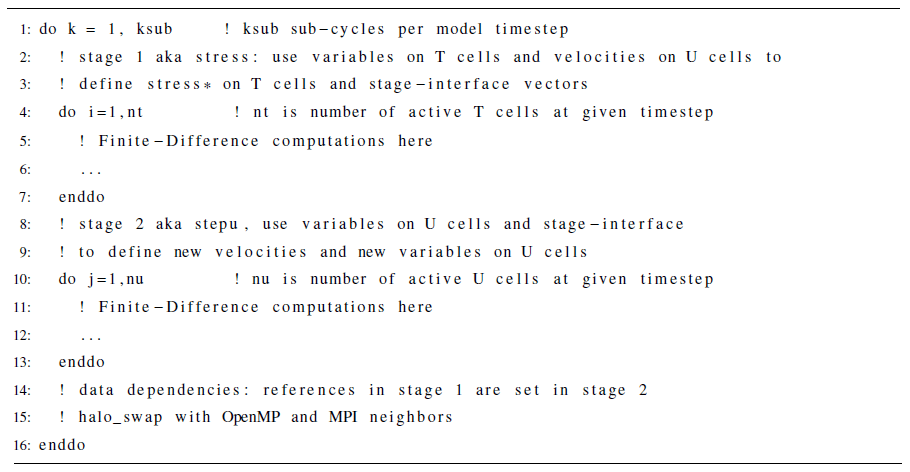
Listing 1 provides a schematic overview of the standard EVP algorithm, which consists of an outer convergence loop, two inner stages (stress and stepu), and a halo swap of the velocities. Each of the inner stages carries an inner loop with its own trip count based on subsets of the active points. The two inner stages within the subcycling exchange arrays are used in the other stage. Therefore, processes or threads must synchronize after each of the stages.

The inner stages operate on a subset of the grid points in 2D space. The grid points are classified as land points, water points, or two types of active ice points, namely U cell points and T cell points, labeled according to the Arakawa definition of the B grid (Arakawa and Lamb, 1977). T refers to the cell center, and U refers to the velocity points at corners. Land and water points are static for a given configuration. Active points are defined by thresholds of the sea ice concentration and the mass of sea ice plus snow. The result is that the number and location of active points may change at every time step, although they remain constant during the subcycling. Most grid cells have both T and U points active, but there are points that only belong to one of these subgroups. For instance, there may be ice in the cell center (T), but the U point lies along a coastline and is therefore inactive. The active sea ice points are always a subset of the water points, changing in time during the simulation due to the change in season and external forcing.

Listing 1 A schematic view of the subcycling of the EVP algorithm.

From a workload perspective, the arithmetic in the EVP algorithm confines itself to short-latency operations: add, mult, div, and sqrt. The computation intensity is 0.3 FLOP (floating-point operations per second) per byte, which makes the workload highly bandwidth-bound. Achieving a well-balanced workload is a huge challenge for any parallel algorithm working on these irregular sets, as was recognized in earlier studies that focus on the performance of CICE (Craig et al., 2015).

2.2 The refactored implementation

This section describes the refactored EVP solver, which was done in two steps. The first focused on improving the core level parallelism, and the second step focused on improving the node level parallelism. The intention of the first step was to establish a solid, single-core baseline before diving into the thread parallelism of the solver.

2.2.1 Single-core refactorization

An important part of the refactorization is changing memory access patterns to reduce the memory bandwidth pressure at the cost of additional floating-point operations. Listing 2 shows a snippet of the standard code (v0) before the first refactorization. The code fragment reveals a classical finite-difference pattern that is similar to the refactorization pattern shown in Chap. 3 of Jeffers and Reinders (2015). The challenge is that compilers see the memory access pattern caused by indirect addressing as random memory access and will consequently refrain from using modern vector (SIMD) instructions in their code generation.

The refactored EVP code is shown in Listing 3. The new solver introduces 1D structures in the place of the original 2D structures, with additional indexing overhead to track the neighboring cells required by the finite-difference scheme. This change allows the compiler to see the memory access pattern as mostly direct addressing, with some indirect addressing required for accessing states in neighboring cells. The compiler will consequently be able to generate SIMD instructions for the loop and will handle the remaining indirect addressing with SIMD gathering instructions. The ratio of indirect $/$ direct memory addressing is 10 %–20 %, depending on which of the two EVP loops is considered. For the Fortran programmer, the two fragments look almost identical, but for the Fortran compiler, the two fragments look very different, and the compiler will be able to convert the latter fragment straight into an efficient instruction set architecture (ISA) representation. The change in data structures from 2D to 1D is the only difference between v0 and v1. The computational intensity of a loop iteration of v0 and v1 is identical.

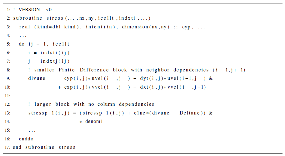
Listing 2 Fragment showing finite-difference dependencies in the standard version of EVP (v0).

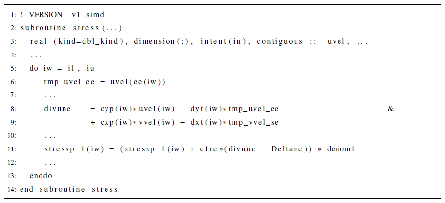
Listing 3 Fragment showing finite-difference dependencies in the refactored version of EVP (v1-simd).

CICE utilizes static grid properties which are computed once during initialization and then re-used in the rest of the simulation. As discussed in the introduction, a sensible strategy reduces bandwidth pressure by adding more pressure on the floating-point engines while reducing memory storage. Our final refactored versions (v2*) have substituted seven static grid arrays with four static base arrays, together with some runtime computations of local scalars, thus deriving all seven original arrays as local scalars; see Listing 4 that shows how the arrays cxp and cyp are derived. The v2* versions are further discussed in Sect. 2.2.2.

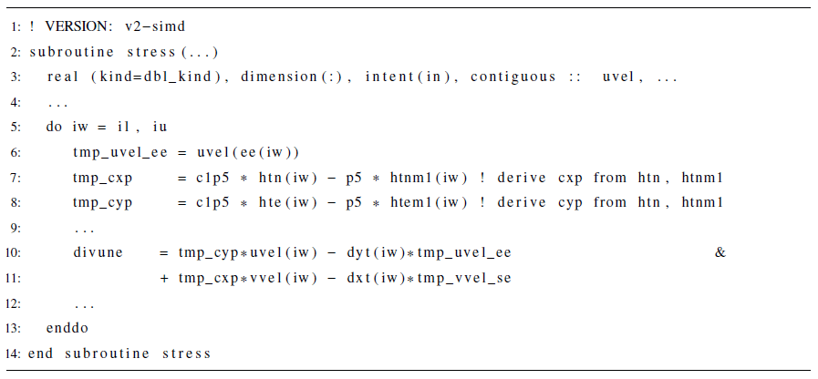
Listing 4 Fragment showing finite-difference dependencies in the refactored version of EVP (v2).

2.2.2 Single-node refactoring – OpenMP and OpenMP target

The existing standard parallelization operates on blocks of active points and elegantly uses the same parallelism for OpenMP and MPI, providing flexibility to run hybrid. It allows for a number of different methods to distribute the blocks onto the computed units to meet the complexity of the varying sea ice cover. There is no support for GPU offloading in the standard parallelization. The refactored EVP kernel demonstrates support for GPU offloading and showcases how this can be done in a portable fashion when confined to open standards. The underlying idea in the OpenMP parallelization is twofold. First, we want to make the OpenMP synchronization points significantly more lightweight than the current standard implementation. The OpenMP synchronization points in the existing implementation involve explicit memory communication of data in the blocks used for parallelization. The proposed OpenMP synchronization only requires an OpenMP barrier to ensure cache coherency and no explicit data movement. Second, we want to increase the granularity of the parallelization unit from blocks of active points to single active points, which will allow better workload balance and scaling when the number of cores is increased.

Keeping the dependencies between the two stages in mind, we have two inner loops that can be parallelized. We must take into account that the T cells and U cells may not be identical sets, and we cannot even assume that one is included in the other. However, it is fair to assume that the difference between the T and U sets of active points is negligible, and instead of treating the two sets as totally independent, we take advantage of their large overlap. Treating the two loops with the same trip count helps the performance tremendously, both in terms of cache and in terms of non-uniform memory access (NUMA) placement. This requires some additional overhead in the code to skip the inactive points in the T and U loops.

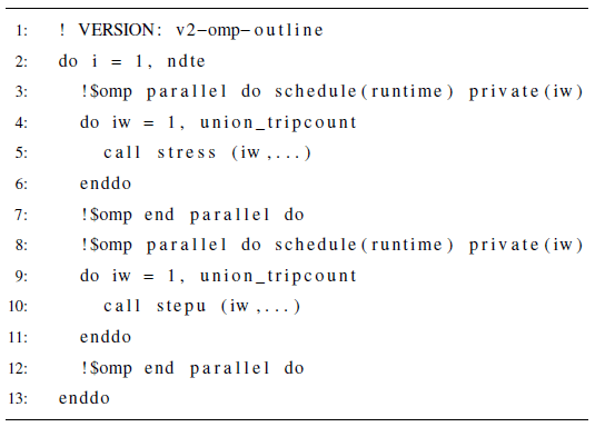
The OpenMP standard published by OpenMP Architecture Review Board (2021) provides several options, and later Fortran standards (Fortran 2008 and Fortran 2018) also provide an opportunity to express this parallelism purely within Fortran. For OpenMP, we can do this either in an outlined fashion (see Listing 5) or in an inlined fashion (see Listing 6).

Listing 5 Fragment showing outlined OpenMP parallelization of EVP (omp-outline).

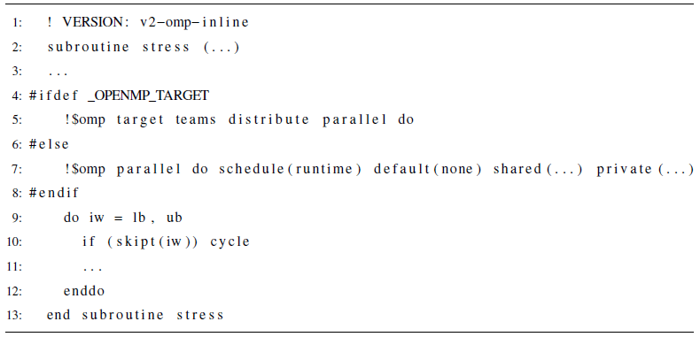
Listing 6 Fragment showing traditional inlined (and OpenMP offloading) OpenMP parallelization of EVP (omp-inline).

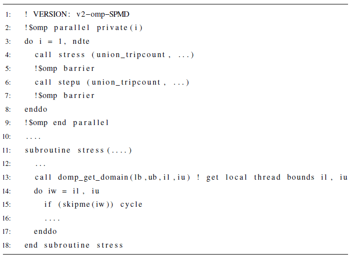
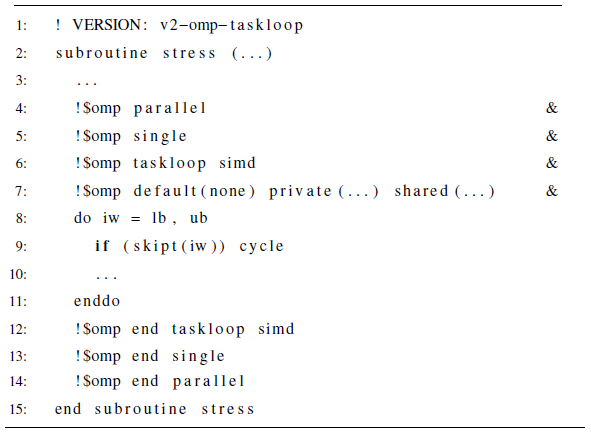
An alternative approach avoids explicit OpenMP runtime scheduling, using OpenMP instead as short-hand notation for handling the spawning of the threads and then manually doing the loop-splitting, as illustrated in Listing 7. We refer to this approach as the single-program, multiple-data (SPMD) approach (Jeffers and Reinders, 2015; Levesque and Vose, 2017). In addition to its simplicity, this approach has the advantage that we can add balancing logic to the loop decomposition, accounting for the application itself and its data. For the sake of completeness, we also parallelize the EVP solver using the newer taskloop constructs available in OpenMP (see Listing 8).

Listing 7 Fragment showing SPMD OpenMP parallelization of EVP (omp-SPMD).

Listing 8 Fragment showing the newer OpenMP taskloop parallelization of EVP (omp-taskloop).

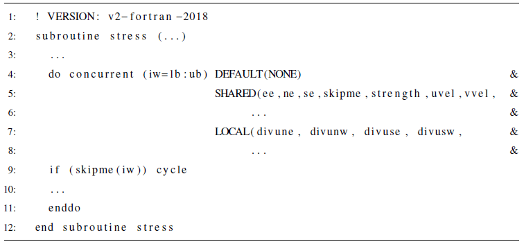
A pure Fortran approach is available with the newer do-concurrent (see Listing 9), and here we may use compiler options to target either the CPU or GPU offloading.

Listing 9 Fragment showing the pure Fortran 2018 approach to parallelism (fortran-2018).

2.3 Test cases

Figure 1 shows the three domains used to test the refactorized EVP solver. Figure 1a is the operational sea ice model domain at DMI (Ponsoni et al., 2023), and Fig. 1b is the Regional Arctic System Model (RASM) domain (Brunke et al., 2018). Both domains cover the pan-Arctic area. These two systems are computationally expensive and are therefore used to analyze, demonstrate, and test the performance of the new EVP solver. Tests are based on restart files from winter (1 March) and summer (1 September), where the ice extent is close to its maximum and minimum, respectively. All performance results shown in this work originate from the RASM domain, which has the most grid points. Neither of these model systems includes boundary conditions, which simplifies the problem.

The gx1 (1°) domain shown in Fig. 1c and d is included to test algorithm correctness and updates to the cyclic boundary conditions. In addition, gx1 is used for testing the numerical noise level for long runs using optimized flags within the CICE test suite. It is not used to evaluate the performance because MPI optimization is beyond the scope of this paper.

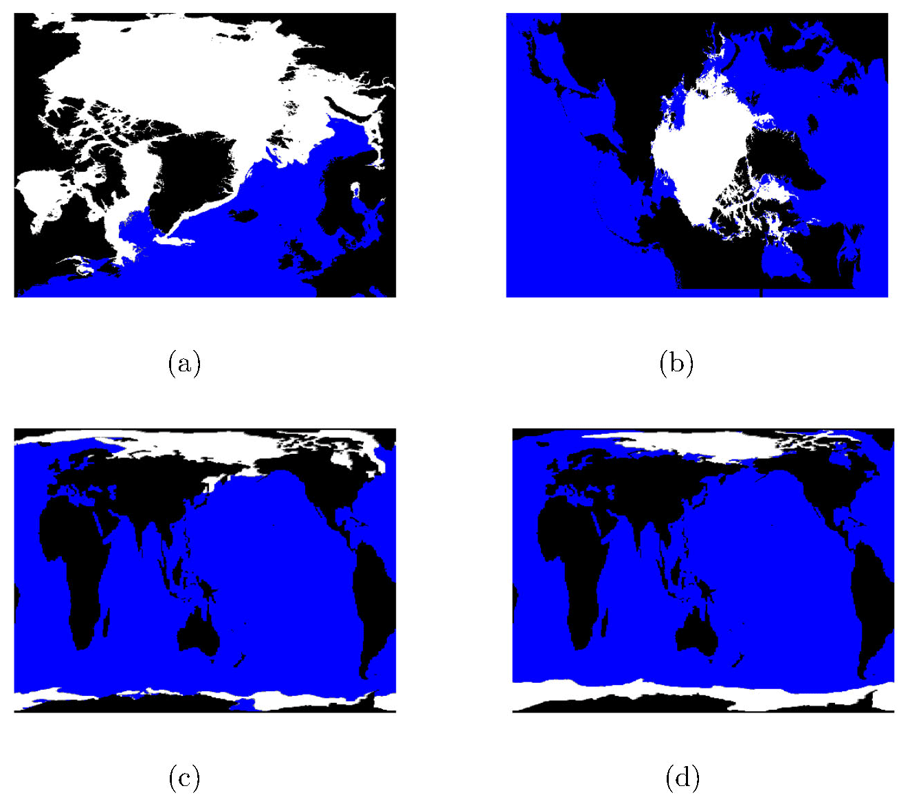
Figure 1 Three domains are used to test the new EVP solver and to verify its integration into CICE. The status of grid points from one restart file for each of the regional domains is shown, and one winter extent and one summer extent are shown for the global domain. (a) The DMI domain on 1 March 2020. (b) The RASM domain on 1 September 2018. (c) The gx1 domain on 1 March 2005. (d) The gx1 domain on 1 September 2005. Black is land, blue is ocean, gray points have either active T or U points, and white points have both T and U points active.

The number of grid points and their classification are listed in Table 1. Figure 1 indicates and Table 1 highlights that most grid points have both T and U points active, confirming our assumption about the design of the refactored EVP solver. However, there are cases in which a grid point can have either a T or a U grid point active.

Table 1 Number of points for the four test domains, with the total number of grid points excluding boundaries, the number of water points, the number of active T and U points (∩), and the number of active T or U points (∪) in winter and summer.

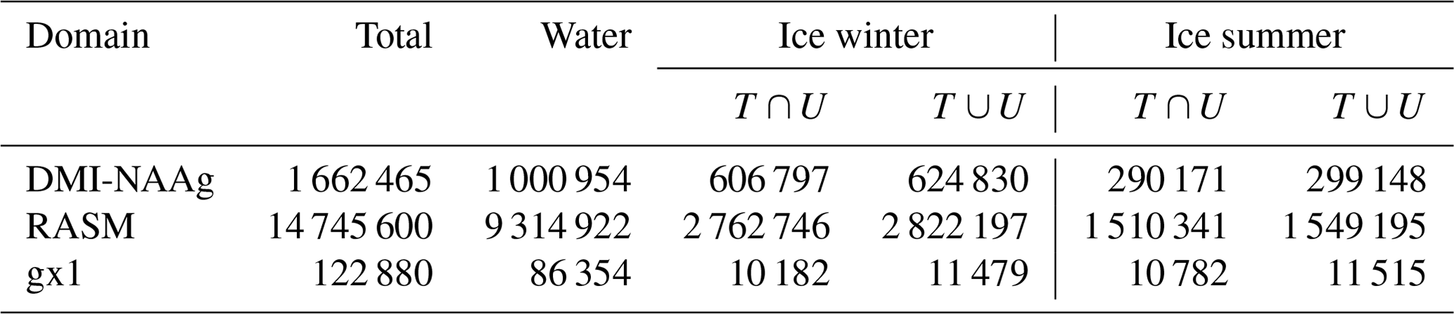
It is clear from Fig. 1 that the variation in the active sea ice points is significant between winter and summer. Table 1 quantifies the variation in the different categories of grid cells. The number of active grid cells varies for the two pan-Arctic domains and is approximately half in summer compared to winter. The minimum and maximum sea ice extent is expected in mid-September and mid-March, respectively. A sinusoidal variation is expected in the period between the minimum and the maximum for the two pan-Arctic domains. The variation is smaller in the global domain, as Antarctica has the maximum number of active points when Arctic is at its minimum, and vice versa. These variations can impact the strategy for the allocation of memory, as one goal is to reduce the memory usage.

Variation in the sea ice cover complicates load balancing when multiple blocks are used. The new implementation of the 1D solver automatically removes all land points and also allows the OpenMP implementation to share memory without synchronization between halos, as opposed to the original 2D OpenMP implementation within CICE.

2.4 Test setup

The performance results in this study are based on a unit test that only includes the EVP solver and not the rest of CICE. Inputs are extracted from realistic CICE runs just before the subcycling of the EVP solver. Validation of the unit test is based on output extracted just after the EVP subcycling. The refactorizations have been tested in three stages (v0, v1, and v2), as described below).

v0

Standard EVP solver.

v1

Single-core refactoring of the memory access patterns used in the EVP solver.

v2

Single-node refactoring illustrating four different OpenMP approaches and one pure Fortran 2018 do-concurrent approach, including conversion from pre-computed grid arrays to scalars recomputed at every iteration.

Unit tests were conducted with different compiler flag optimizations ranging from very conservative to very aggressive, where v0 is the baseline, and the performance of v1 and v2 has been compared to this. A weak scaling feature has also been added to the standalone test in order to measure the performance at different resolutions/numbers of grid points and to allow for full node performance tests.

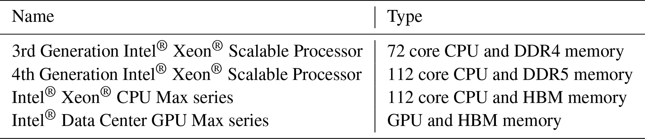
The refactorization and its impact on performance has been tested on four types of architectures (Table 2) to demonstrate the effect of the bandwidth limitation and the performance enhancement on CPUs and GPUs. All CPU executables were built using the Intel^® Classic Fortran compiler, and all the GPU executables were built with the Intel^® Fortran compiler from the oneAPI HPC toolkit 2023.0. All implementations use only open standards without proprietary extensions. Therefore, we expect that similar results can be achieved on hardware from other providers than Intel.

Table 2 Description of the CPUs and the GPU used in this study. Hardware listed with HBM includes high-bandwidth memory. More information can be found at https://www.intel.com/content/www/us/en/products/overview.html (last access: 27 August 2024).

All performance numbers reported are the average time obtained for 10 test repetitions using omp_get_wtime(). Timings do not include the conversion from 1D to 2D, and vice versa. For the capacity measurements, eight ensemble members run the same workload simultaneously and are evenly distributed across the full node, device, or set of devices. The timing of an ensemble run is the time of the slowest ensemble member; we repeat the ensemble runs 10 times and report the average. All performance experiments on the 4th Generation Intel^® Xeon^® Scalable Processor and Intel^® Xeon^® CPU Max series are done in SNC4 mode and with HBM only on Intel^® Xeon^® CPU Max series.

The GPU results indicate only the computed part and not the usually time-consuming data traffic between the CPU and the GPU. Because the kernel constitutes a single model time step, most data traffic in this kernel has a one-time initialization and hence would not contribute to the computing time in the N−1 remaining time steps of a full simulation.

Finally, one of the v2 refactored units was integrated back into CICE (Hunke et al., 2024). This initial integration is focused solely on correctness. Section 4 presents our proposal of a performance-focused integration, which can be considered a refactorization at the cluster level that is on top of the refactoring at the core and node levels reported here.

The new method does not include any new physics. Therefore, it is important that the results remain the same. This is verified by checking that restart output files contain “bit-for-bit” identical results at the end of two parallel simulations, which require identical md5sums on non-optimized code. All tests verify this (not shown). It should be noted that the baseline v0 cannot be run on a GPU, since the baseline code only supports building for CPU targets. Therefore, it is not possible to cross-compare the GPU baseline results with refactored GPU results. The GPU results were compared with the refactored CPU with no expectation of bit-for-bit identical results.

When the build of the binary executable uses more aggressive compiler optimization flags, it may use operations that produce a different final rounding-off error. It may also do exactly the same calculations in another order, which results in bit-for-bit differences due to the discrete representation of real numbers. For instance, a fused multiply–add operation has one rounding operation, whereas the same calculation can be represented by one multiplication followed by an addition that results in two rounding operations. Such a deviation does not originate from differences in the semantics dictated by the source code itself, which expresses exactly the same set of computations. The difference originates from the ability of the compiler to choose from a larger set of instructions. For the optimized, non-bit-for-bit v2 that is integrated into CICE, it is verified that the numerical noise is at an acceptable level with a quality control (QC) module (Roberts et al., 2018) provided with the CICE software. The CICE QC test checks that two non-identical ice thickness results are statistically the same, based on 5-year simulations on the gx1 domain. The result is shown in Fig. 2. The refactored code passes the QC test when integrated into CICE because the noise level is lower than the test's criterion.

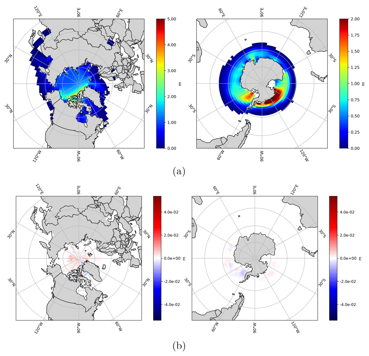
Figure 2 (a) Sea ice thickness on the Northern Hemisphere. (b) Sea ice thickness on the Southern Hemisphere. (c) Difference between CICE using the standard EVP solver (v0) and the refactored EVP solver (v2) implemented into CICE on the Northern Hemisphere. (d) Difference between CICE using the standard EVP solver (v0) and the refactored EVP solver (v2) implemented into CICE on the Northern Hemisphere. All results represent 1 January 2009 after 5 years of simulation starting on 1 January 2005 and using the gx1 grid provided by the CICE Consortium.

3 Performance results

There are several ways to measure and evaluate computing performance. This section focuses on evaluating the EVP standalone kernel performance as measured by the time to the solution on different computing nodes. The evaluation is split into two steps, namely single-core performance and single-node performance.

3.1 Single-core performance

The motivation for the single-core refactorization described in Sect. 2.2.1 is to allow the compiler to utilize vector instructions, also known as single-instruction, multiple-data (SIMD) instructions, instead of confining the program to x86 scalar instructions for both memory accesses and math operations. The instruction sets, formally known as AVX-2 (256 bits) and AVX-512 (512 bits), constitute two newer generations of SIMD to the x86 instruction set architecture for microprocessors from Intel and AMD. Compiler options can be used to specify specific versions of SIMD instructions, but the compiler can only honor this request if the code itself is SIMD vectorizable. One requirement for SIMD vectorization is direct memory rather than random memory access.

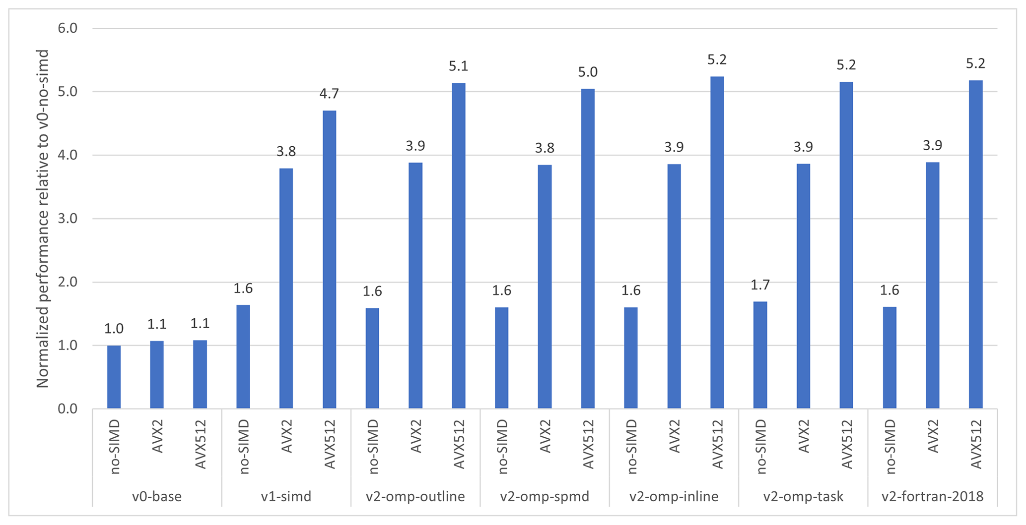
Figure 3 Single-core 3rd Generation Intel^® Xeon^® Scalable Processor (8360y) performance for the same algorithm (EVP) implemented via different approaches and with the build process requesting no SIMD or AVX2 and AVX512 code generation. The prefix versions v0, v1, and v2 are defined in Sect. 2.4, and the baseline is the original implementation (v0) without SIMD generation. Each bar shows the improvement factor compared to the baseline.

Figure 3 shows the single-core performance of the different EVP implementations described in Listings 2–3 and Listings 5–9 for the RASM domain described in Table 1. The upstream implementation (v0) shows limited improvement when applying either AVX-2 or AVX-512, as described in Sect. 2. The improvement factor for the single-core refactorization is approximately 1.6 when SIMD instructions are not used for building v1 and v2*. When SIMD is used, the improvement factor increases to 3.8 for AVX2 and 5.1 for AVX512 code generation. Moreover, the SIMD improvements are achieved across the different OpenMP versions. Although all the refactored versions show the same performance, this is not given a priori, since the intermediate code representation given to the compiler back-end is expected to be different for each of these representations. The refactorization from 2D to 1D changes the memory access from random to direct, allowing the compiler to use the SIMD instructions.

The results from the simulations on the single core show that the refactorization improves the code generation and associated performance. In addition, the one-dimensional compressed memory footprint is much more efficient that the standard two-dimensional block structure, since it reduces the memory footprint by the ratio of ice points to grid points. For the RASM case, it amounts to a factor of 5 reduction in winter and 10 in summer (see Table 1). Importantly, all points in the 2D arrays used in the standard implementation must be allocated, whereas the refactored data structure only needs the active points allocated.

3.2 Single-node performance

Efficient node performance requires that an implementation has both good single-core performance and good scaling properties. The main target of this section is to describe the performance results as measured by the time to the solution on a given node architecture. The performance diagrams found in this section show the performance outcome when all the cores available on the node or device are used. The refactored code is ported to GPUs using OpenMP target offloading. For the capacity scaling study, this allows us to run on hosts that support multiple GPU devices, but we have confined the strong scaling study to classical OpenMP offloading, which currently only supports single-device offloading (see Raul Torres and Teruel, 2022).

In addition, single-node performance is measured according to the relevant hardware metrics. Because the EVP implementation is memory-bandwidth-bound, it is relevant to compare the sustained bandwidth performance of EVP with the well-established bandwidth benchmark STREAM Triad (see McCalpin, 1995, and Fig. 4). The STREAM Triad benchmark delivers a main memory bandwidth number (measured in Gb s⁻¹) and is considered to be the practical limit sustainable on the system being measured.

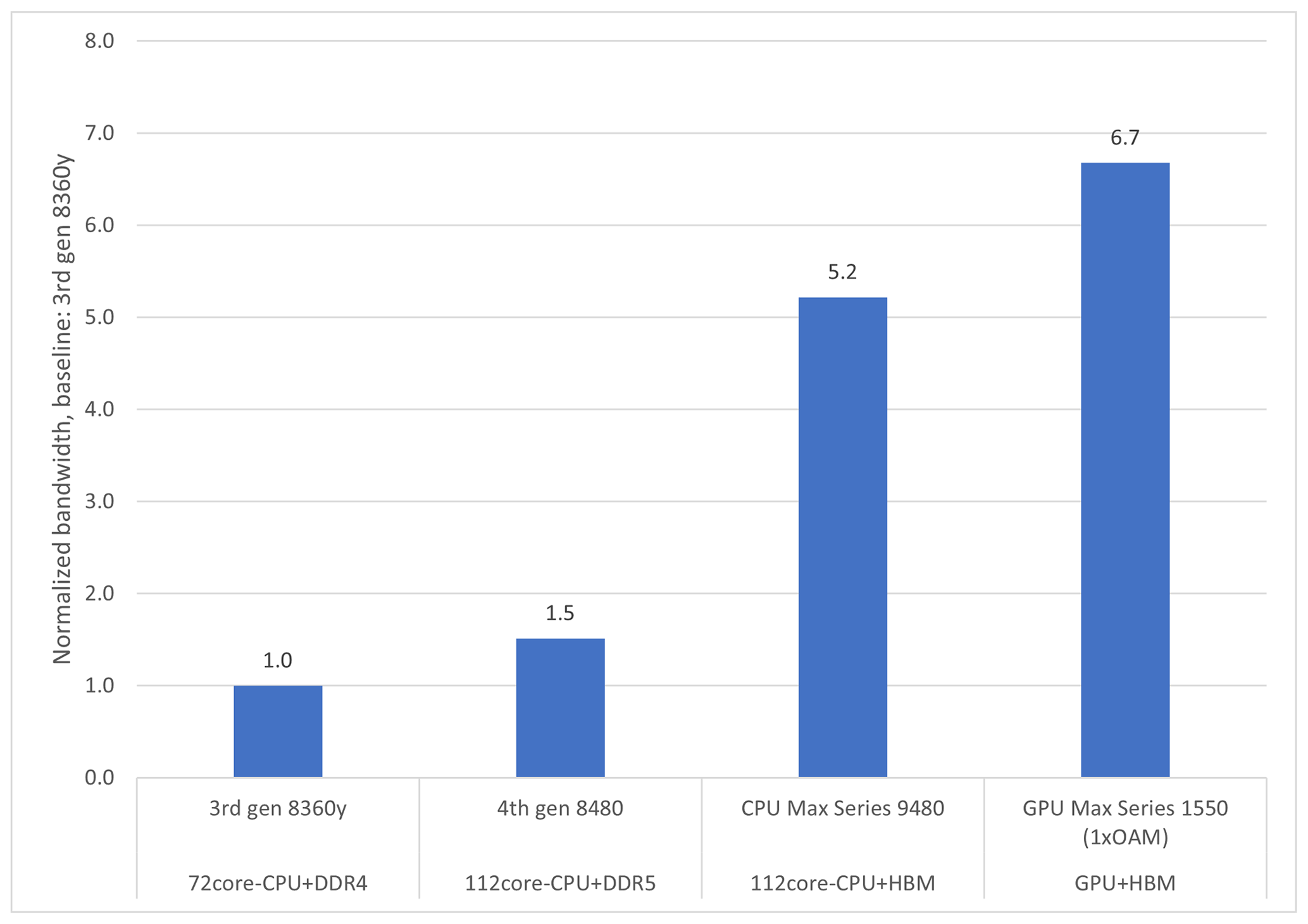
Figure 4 The figure shows the improvement factor for the STREAM Triad memory bandwidth benchmark on different hardware, indicating what is achievable at best for solely bandwidth-bound code. From left to right, the bars are the baselines based on the 3rd Generation Intel^® Xeon^® Scalable Processor, the 4th Generation Intel^® Xeon^® Scalable Processor, Intel^® Xeon^® CPU Max series, and Intel^® Data Center GPU Max series (see Table 2).

Section 3.2.1 focuses on performance results for a strong scaling study, whereas Sect. 3.2.2 focuses on capacity scaling. Single-node performance is evaluated on the architectures described in Table 2. The measured performance is compared to STREAM Triad benchmarks. This indicates whether the algorithm utilizes the full bandwidth of the hardware. Numbers are compared for usage of the full node.

3.2.1 Strong scaling

Strong scaling is defined as the ability to run the same workload faster using more resources. The ability to strong-scale any workload is described by Amdahl's law (Amdahl, 1967).

Figure 5a shows the impact of the choice of architecture on the single-node performance results of the refactored EVP code for the four architectures described in Table 2. Note that the 3rd Generation Intel^® Xeon^® Scalable Processor only has 72 cores. The improvement factor between the CPUs with double-data rate (DDR)-based memory coincides with the improvement factor obtained by STREAM Triad (Fig. 4), which is considered the practical achievable limit of the hardware. The improvement factor for the two bandwidth-optimized architectures (Intel^® Xeon^® CPU Max series and Intel^® Data Center GPU Max series) is less than the corresponding improvement factor obtained by STREAM Triad. This indicates that bandwidth to memory is no longer the limiting performance factor. This finding will be discussed further in Sect. 4.

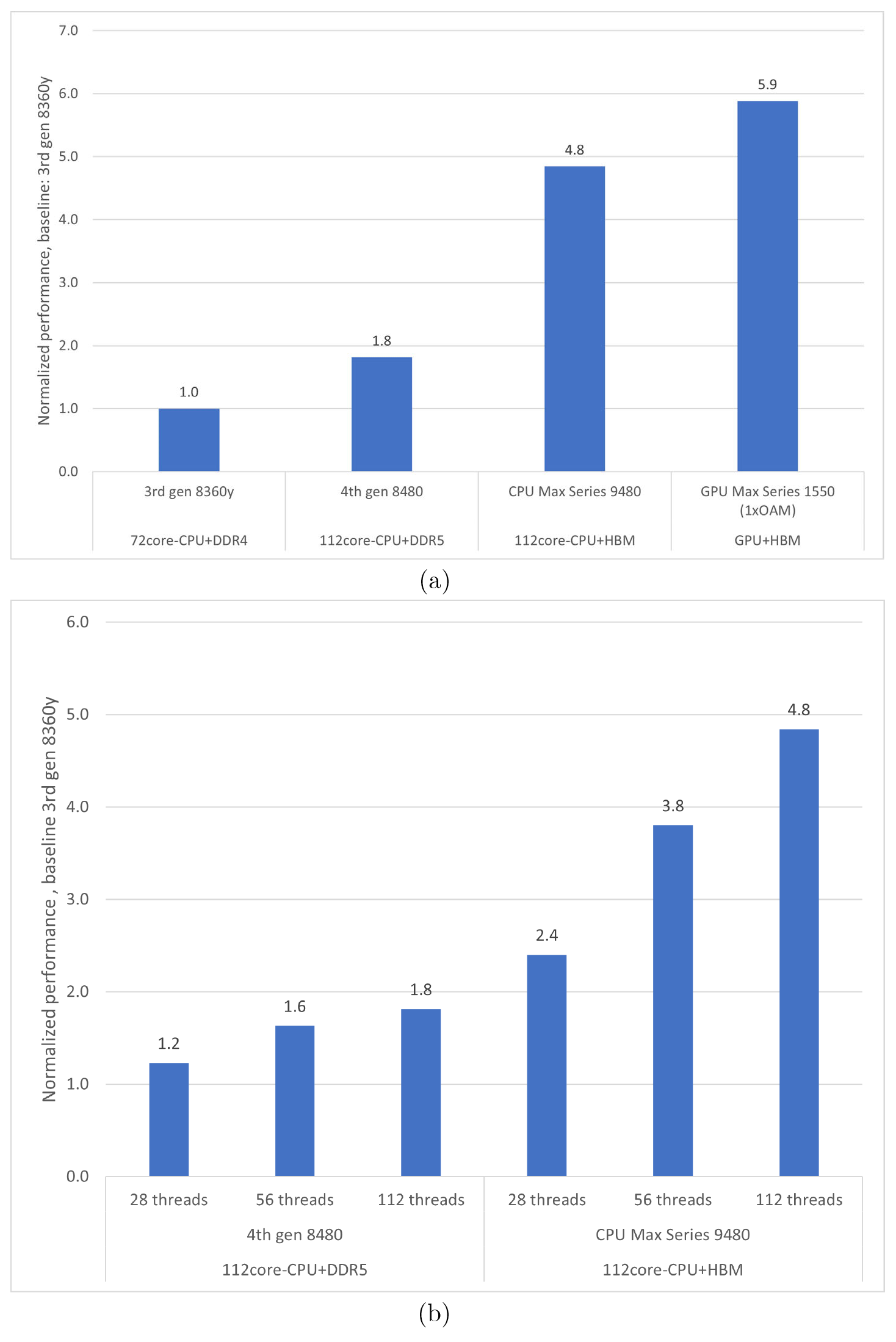
Figure 5 Improvement factors for the refactored EVP code (v2). (a) Strong scaling performance when using all available cores on one node for each of the four hardware types. Shown from left to right are the 3rd Generation Intel^® Xeon^® Scalable Processor, the 4th Generation Intel^® Xeon^® Scalable Processor, Intel^® Xeon^® CPU Max series, and Intel^® Data Center GPU Max series (see Table 2). (b) Strong scaling performance at three different core counts for the 4th Generation Intel^® Xeon^® Scalable Processor and Intel^® Xeon^® CPU Max series. The baseline for panels (a) and (b) is the performance of the 3rd Generation Intel^® Xeon^® Scalable Processor when using all cores.

Figure 5b shows the performance at different core counts for the two hardware types (4th Generation Intel^® Xeon^® Scalable Processor and Intel^® Xeon^® CPU Max series) that are similar except for their bandwidth. The first observation is that the performance of the HBM-based CPU is better than that of the DDR-based CPU. The second observation is that the DDR-based hardware performance stops improving at approximately half the number of cores available on the node, which prevents further scaling on that memory system. With the HBM hardware, the code scales out to all the cores on the node. The improvement factor differs because the sustained bandwidth becomes saturated on the 4th Generation Intel^® Xeon^® Scalable Processor memory. This underlines the importance of the code refactorization to reduce the pressure on the bottleneck, which, in this case, is the bandwidth. It also illustrates that the hardware sets the limits for the potential optimization.

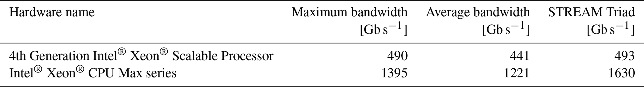
Strong scaling performance is also measured for bandwidth in absolute numbers in Table 3. The absolute bandwidth measurements confirm that the DDR-based memory obtains the same bandwidth as STREAM Triad, whereas the HBM-based CPUs do not utilize the full bandwidth.

Table 3 Absolute measurements of memory bandwidth for strong scaling.

If both the standard and the new implementations of the EVP solver strongly scale equally well, then the node improvement factor should be the same as the single-core improvement factor found in Sect. 3.1. The observed improvement factors of refactored versus standard EVP on the 4th Generation Intel^® Xeon^® Scalable Processor and Intel^® Xeon^® CPU Max series are 13 and 35 (not shown), respectively; i.e., the new EVP solver also scales better than the original EVP implementation on both systems. The standard EVP code allows for multiple decompositions, which may affect the result, but the conclusions remain the same.

3.2.2 Capacity scaling

Capacity scaling is defined as the ability to run the same workload in multiple incarnations (called ensemble members) simultaneously on multiple computing resources. Perfect capacity scaling is achieved when we can run N ensemble members on N computing resources, with a performance degradation bounded by the run-to-run variance measured when running one ensemble member on one computing resource and leaving the rest of the computing resources idle. This performance metric indicates how sensitive the performance is to what is being executed on the neighboring computing resources.

Table 4 shows the absolute numbers and the output from the STREAM Triad test for capacity scaling. The capacity scaling is perfect on the DDR-based systems; i.e., the variance of the timings between individual ensemble members is similar to the variation in timings of repeated single-member runs.

Table 4 Absolute measurements of memory bandwidth for capacity scaling.

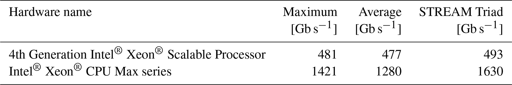
Figure 6 summarizes the capacity scaling results, highlighting how well the different types of hardware perform compared to the best-known achievable bandwidth estimates, which are based on STREAM Triad. The improvement factor between the two DDR-based systems again coincides with the improvement factor obtained by STREAM Triad, which means that the performance is bandwidth-bound. The improvement factor for the bandwidth-optimized architectures is somewhat less than the corresponding improvement factor obtained by STREAM Triad. This is discussed further in Sect. 4.

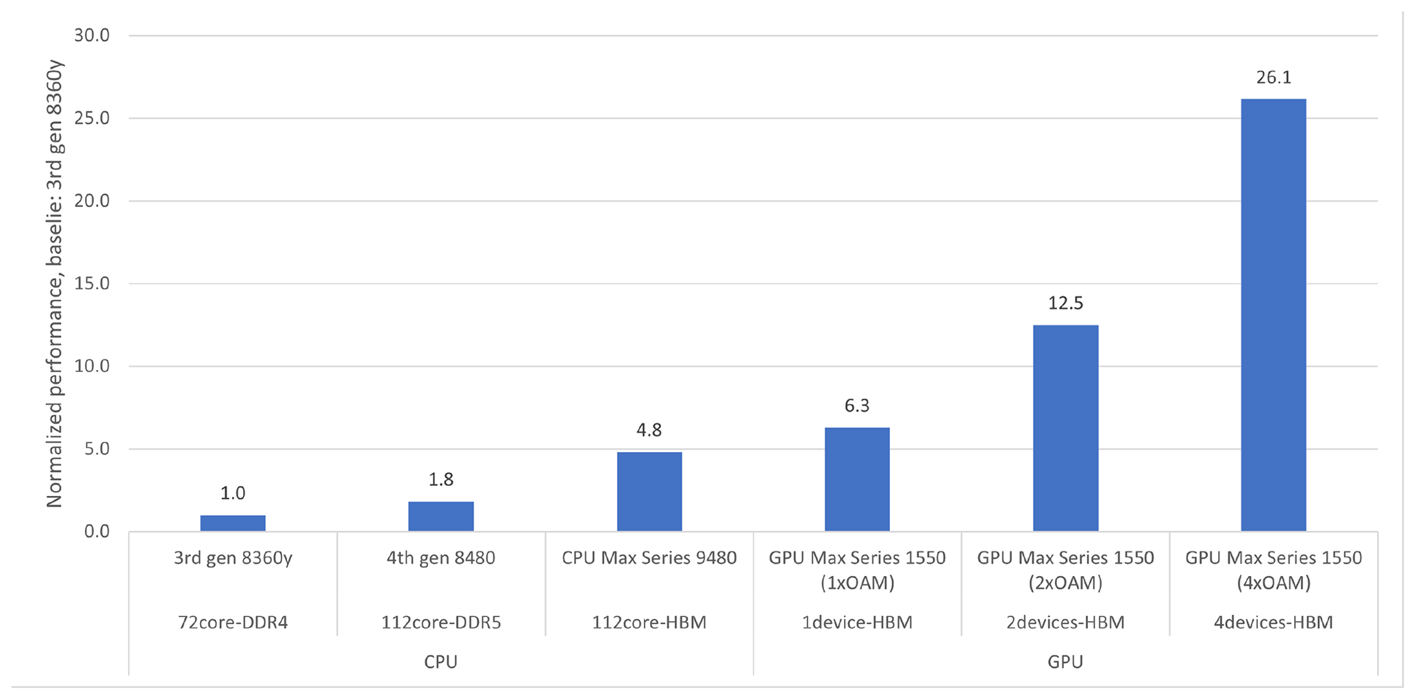
Figure 6 Capacity scaling performance of the refactored EVP unit test, normalized to the 3rd Generation Intel^® Xeon^® Scalable Processor (3rd Generation 8360y) node baseline, which sustains the same bandwidth as STREAM Triad. The figure also illustrates how much using one, two, or four GPU devices per node matters to the collected node throughput.

HPC systems with GPUs typically host multiple devices per node, and this is the reason that we have conducted a multi-device experiment. The experiment shows that the performance continues to increase, but the energy required to drive a node with four GPU devices is significantly higher than the energy required to drive the dual-socket CPU with which we cross-compare. Our intent is not to compare the CPUs and GPUs directly because other elements such as energy or price should be considered.

4 Discussion

These results demonstrate a refactorization of the EVP solver within CICE that takes full advantage of modern CPUs and GPUs. All performance tests are based on an EVP solver unit test, as described in Sect. 2.4. The new implementation is easy to adapt to an unstructured grid, although it is implemented here on a structured grid. There were choices both in the refactorization of the EVP solver and in its integration into CICE, which are discussed in this section.

The new single-core SIMD parallel performance and the new single-node OpenMP parallel performance are evaluated in the previous sections. Based on comparisons with STREAM Triad, the refactored code reaches the peak bandwidth performance of the two DDR-based memory systems, but the peak bandwidth of the HBM-based system is not reached. On the Intel^® Xeon^® CPU Max series with HBM running in HBM-only mode, we reached ≈80 % of the practical peak bandwidth. This result is consistent for both capacity scaling and strong scaling. Although the improvement factor is the same for both types of scaling, the reasons for the performance gap are quite different. The strong scaling gap for the Intel^® Xeon^® CPU Max series CPU is solely due to limitations in the algorithm and data set, where there is an inherent imbalance.

The capacity scaling issue is that the hardware enforces a lower frequency (both core and uncore) to ensure that it does not overheat when all NUMA domains operate simultaneously. A drop in the core frequency results in a slowing down of the computations. In addition, the reduction in the uncore frequency causes higher memory latency. STREAM Triad does not include the effects enforced by the hardware. For this reason, the STREAM Triad benchmark is too simple for the bandwidth-optimized CPU.

The first integration step described in this study uses the current infrastructure within CICE and focuses solely on correctness, not on the performance, in order to establish a solid foundation for future work. For instance, the implementation utilizes existing gathering/scattering methods to convert some of the arrays from 1D and 2D global to a 3D block structure (and vice versa), which is used for parallelization in the rest of the CICE code. It would be better to convert the 1D arrays directly to the block structure (1D to 3D). The number of calls to gathering/scattering methods could also be reduced. The ideal solution would be for all spatial quantities to only exist as 1D vectors; most EVP loops are already geared towards this, as they loop in 1D space with pointers to the two indices used in the array allocation. The halo swaps could be re-introduced directly on the new 1D data structures using MPI-3 neighborhood collectives.

A major performance challenge within the standard EVP solver is the set of halo updates required at every EVP subcycle since each halo update introduces an MPI synchronization. Better convergence is achieved when the number of subcycles increases, but this also linearly increases the number of MPI synchronizations. The goal is to improve the performance of the full model; therefore, the number of synchronizations must be reduced.

The initial integration of the refactored EVP code into CICE only allows MPI synchronizations at the time step level. This prevents CICE from being split into subcomponents, as suggested below, and it requires the same number of threads for the refactored EVP as for the rest of CICE. The refactored EVP will consequently only be able to utilize a single MPI task, leaving the remaining MPI tasks idle. This is obviously a very inefficient integration that retains the observed scaling challenge at the cluster level.

To improve the initial integration performance and to cope with the underlying challenges, an alternative approach is suggested that leverages multiple-program, multiple-data (MPMD) parallelization (Mattson et al., 2005). This allows heterogeneous configurations, where the EVP solver could run on separate hardware resources and/or utilize different parallelization strategies (e.g., pure MPI, hybrid OpenMP–MPI, and hybrid OpenMP–MPI running OpenMP offloading) relative to the rest of the model. If a time lag is implemented between the two components, then they could run concurrently. This approach is also beneficial for the performance of the rest of the model, as it relieves the model from carrying EVP state variables and prevents flushing the cached EVP state at every time step. It would also allow runs of several EVP ensemble members on a single node, thereby serving a set of model ensemble members each running on their own set of nodes. Also, it would be easier to integrate the new EVP component into other modeling systems because it will have a pure-MPI interface.

The MPMD pattern is generally used by ESM communities for load-balancing coupled model systems, e.g., where the ocean and the sea ice model run on different groups of the cores or nodes (e.g.,  Ponsoni et al., 2023; Craig et al., 2012). Sometimes MPMD is used internally within systems for input/output (I/O) (e.g., the ocean model, NEMO; Madec et al., 2023). To the best of our knowledge it is not common to use the MPMD pattern for model subcomponents beyond I/O handling, nor is it common for it to support heterogeneous systems.

This new implementation of the EVP solver within CICE includes a strategy involving how to allocate data. The strategy selected for this integration is to allocate all ocean points and then check whether or not they are active within the calculations. For the domains in this study, this strategy induces a large overhead, since there are many ocean points that are never active (see Table 1). However, this behavior is domain-specific and will be very different for different setups. A second strategy could be to reallocate all 1D vectors at every time step and only allocate the active points. This induces an overhead for reallocating at every time step, but it reduces the memory usage. An alternative, intermediate method would be to only reallocate when the number of active points increases above what has been allocated. We propose this last strategy for the final MPMD-based MPI refactoring in CICE.

5 Conclusions

This study analyzed the performance of the EVP solver extracted from the sea ice model (CICE) and found performance challenges with the standard parallelization options at the core, node, and cluster levels. An evaluation of the refactorized solver demonstrates significant performance and memory footprint improvements.

The refactored EVP code improved performance by a factor of 5 compared to the original version when one core is used on the 3rd Generation Intel^® Xeon^® Scalable Processor. This improvement is primarily the result of a change in the memory access patterns from random to direct, which allows the compiler to utilize vector instructions such as SIMD. When using 112 cores (full node), the improvement factor on the 4th Generation Intel^® Xeon^® Scalable Processor is 13, and on the Intel^® Xeon^® CPU Max series it is 35. The study showed that the limiting performance factor for EVP on traditional CPUs is the memory bandwidth. This is the main difference between the two types of hardware and the main reason for the difference in performance on a full node.

The refactored version is capable of sustaining the STREAM Triad bandwidth (practical peak performance) on the CPUs within this study that is based on DDR-based memory. For strong scaling on the Intel^® Xeon^® CPU Max series, only 80 % of the bandwidth was used due to imbalances in the algorithm and the data sets. Finally, GPUs deliver higher memory bandwidth than CPUs, so we also ported the new implementation to nodes with GPU devices. All CPU and GPU performances were achieved solely using open standards, OpenMP, and oneAPI in particular.

The single-node improvements were integrated into the CICE model to check simulation correctness. Our next step will be to improve the integrated code, focusing on full model performance for both CPUs and GPUs.

Appendix A: Abbreviations

CICE	The Los Alamos sea ice model
DMI	Danish Meteorological Institute
DDR	Double-data rate
ESM	Earth system model
EVP	Elastic–viscous–plastic
HBM	High-bandwidth memory
MPMD	Multiple program, multiple data
NUMA	Non-uniform memory access
QC	Quality control
RASM	Regional Arctic system model
SIMD	Single instruction, multiple data
SPMD	Single program, multiple data
VP	Viscous–plastic