Towards a real-time modeling of global ocean waves by the fully GPU-accelerated spectral wave model WAM6-GPU v1.0

The spectral wave model WAM (Cycle 6) is a commonly used code package for ocean wave forecasting. However, it is still a challenge to include it into the long-term Earth system modeling due to the huge computing requirement. In this study, we have successfully developed a GPU-accelerated version of the WAM model that can run all its computing-demanding components on GPUs, with a significant performance increase compared with its original CPU version. The power of GPU computing has been unleashed through substantial efforts of code refactoring, which reduces the computing time of a 7 d global $\mathrm{1}/\mathrm{10}$° wave modeling to only 7.6 min in a single-node server installed with eight NVIDIA A100 GPUs. Speedup comparisons exhibit that running the WAM6 with eight cards can achieve the maximum speedup ratio of 37 over the dual-socket CPU node with two Intel Xeon 6236 CPUs. The study provides an approach to energy-efficient computing for ocean wave modeling. A preliminary evaluation suggests that approximately 90 % of power can be saved.

1 Introduction

Ocean wave modeling has long been regarded as an important part of numerical weather prediction systems due to not only its critical role in ship routing and offshore engineering, but also its climate effects (Cavaleri et al., 2012). Nowadays, wave forecasts are generated from the spectral wave models routinely operating on the scale of ocean basins to continental shelves (Valiente et al., 2023). To assess the uncertainty in wave forecasts, major national weather prediction centers also adopt an ensemble approach to provide probabilistic wave forecasts (Alves et al., 2013). For example, the Atlantic Ensemble Wave Model of the Met Office issues probabilistic wave forecasts from an ensemble of 36 members at a 20 km resolution. However, due to the limitation of the high-performance computing (HPC) resource, these ensemble members have to be loaded in two groups with a latency of 6 h for each (Bunney and Saulter, 2015). Increasing the spatial resolution and conducting ensemble forecasting both require significant HPC resources (Brus et al., 2021).

In recent decades, wind-generated surface waves are revealing themselves more and more as the crucial element modulating the heat, momentum, and mass fluxes between ocean and atmosphere (Cavaleri et al., 2012). The air–sea fluxes of momentum and energy are sea-state-dependent, and the forecasts of winds over ocean are demonstrably improved by coupling atmosphere and wave models. Ocean circulation modeling can also be improved through coupling with wave models (Breivik et al., 2015; Couvelard et al., 2020). Waves absorb kinetic energy and momentum from the wind field when they grow and in turn release it when they break, thus significantly enhancing the turbulence in the upper mixing layer (Janssen, 2012). Non-breaking waves and swells stir the upper water and produce enhanced upper-layer mixing (Huang et al., 2011; Fan and Griffies, 2014). For high-latitude marginal ice zones (MIZs), ice–wave interactions comprise a variety of processes, such as wave scattering and dissipation and ice fracturing, which also have important impacts on both atmospheric and oceanic components (Williams et al., 2012; Iwasaki and Otsuka, 2021). The Earth system model (ESM) developers are making efforts to explicitly include a surface wave model into their coupling framework. For example, as part of ECMWF’s Earth system, the wave model component of the IFS is actively coupled with both the atmosphere and the ocean modeling subsystems (Roberts et al., 2018). The First Institute of Oceanography Earth System Model (FIO-ESM; Qiao et al., 2013; Bao et al., 2020) and the Community Earth System Model version 2 (Danabasoglu et al., 2020; Brus et al., 2021; Ikuyajolu et al., 2024) also include a spectral wave model as part of their default components.

The spectral wave models resolve wave phenomenons as a combination of wave components along a frequency and direction spectrum across space and time. Their generation, dissipation, and nonlinear interaction processes are described by a wave action transport equation with a series of source terms, which requires large computational resources and a long computing time (Cavaleri et al., 2007). The first operational third-generation spectral model, WAM (WAve Modeling), was developed in 1980s (The Wamdi Group, 1988). WAM has been replaced by the WaveWatch III (Tolman, 1999) as the most commonly used global and regional wave model used by major national weather prediction (NWP) centers. The SWAN (Simulating WAves Nearshore), is also a popular wave model which has advantages in nearshore regions (Booij et al., 1999). All these wave models are under continued development by different communities, and their code packages are freely accessible.

As an efficient and portable yet commercially available substitute for HPC clusters, GPU computation has played a central role in implementing massive computation power across a wide range of areas (Yuan et al., 2020, 2023). In the area of ocean and climate modeling, a variety of mainstream models and algorithms have been successfully ported to GPU devices, with substantial improvement on model performance being reported (Xiao et al., 2013; Xu et al., 2015; Qin et al., 2019; Yuan et al., 2020; Jiang et al., 2019; Häfner et al., 2021). For brevity, in this paper, we do not elaborate on these pioneering works. Due to the complexity of code, GPU acceleration of spectral wave models has not been reported in public until recently. Ikuyajolu et al. (2023) has ported one of the WaveWatch III’s source-term scheme W3SRCEMD to GPU with OpenACC. However, the GPU implementation only exhibited a 35 %–40 % decrease in both simulation time and usage of computational resources, which was not satisfactory. They suggested that rather than a simple usage of OpenACC routine directives, a significant effort on code refactoring had to be done for better performance.

Since 2020, we have managed to fully port the WAM Cycle 6 wave model to GPUs through a significant amount of work. The purpose of this paper is to report the progress that has been made. The paper is organized as follows. Section 2 briefly reviews the governing equations and physical schemes adopted by WAM; Then, the OpenACC implementation of the model and optimization strategies are detailed in Sect. 3. Performance analysis through a global high-resolution wave hindcast is made in Sect. 4. A brief summary is presented in Sect. 5.

2 Wave model WAM

The ocean wave model WAM is a third-generation wave model that describes the evolution of the wave spectrum by solving the wave energy transport equation. In this study, WAM Cycle 6 (hereinafter referred to as WAM6) is adopted. WAM6 is one of the outcomes of the MyWave project funded by the European Union (EU), which brings together several major operational centers in Europe to develop a unified European system for wave forecasting based on the updated wave physics (Baordo et al., 2020). Generally, the third-generation wave models are based on the following wave action balance equation in spherical coordinates (Eq. 1):

$$\begin{array}{}\text{(1)}& \begin{array}{rl}{\displaystyle \frac{\partial }{\partial t}}N& +\left(\cos \mathit{\varphi }{)}^{-\mathrm{1}}{\displaystyle \frac{\partial }{\partial \mathit{\varphi }}}\right(\dot{\mathit{\varphi }}\cos \mathit{\varphi }N)+{\displaystyle \frac{\partial }{\partial \mathit{\lambda }}}(\dot{\mathit{\lambda }}N)+{\displaystyle \frac{\partial }{\partial \mathit{\omega }}}(\dot{\mathit{\omega }}N)\\ & +{\displaystyle \frac{\partial }{\partial \mathit{\theta }}}\left(\dot{\mathit{\theta }}N\right)=S_{\mathrm{in}}+S_{\mathrm{ds}}+S_{\mathrm{nl}}+S_{\mathrm{bot}}+S_{\mathrm{brk}}.\end{array}\end{array}$$

The left-hand side of Eq. (1) accounts for spatial and intra-spectrum propagation of spectral wave energy along two-dimensional (2D) geographic space (ϕ for latitude and λ for longitude), angular frequency (ω) and direction (θ), respectively. The five terms on the right-hand side of Eq. (1) are source terms, which represent the physics of wind input (S_in), dissipation due to whitecapping (S_ds), nonlinear wave–wave interaction (S_nl), bottom friction (S_bot), and depth-induced wave breaking (S_brk). Two sets of wave physics parameterizations, which are based on the works of Janssen (1989, 1991) and Ardhuin et al. (2010), are available in WAM6. A first-order upwind flux scheme is used for advection terms, and the source terms are integrated using a semi-implicit integration scheme. For the full description of the governing equation, parameterization and numerical schemes, one can refer to ECMWF (2023), Günther et al. (1992), and Behrens and Janssen (2013).

The flow diagram of the WAM6 model is illustrated in Fig. 1. The WAM6 model has a pre-processing program (PREPROC), which generates the computing grids with two alternative options. The default option is to produce a reduced Gaussian grid. In this case, the number of grid points along the latitude reduces poleward with east–west grid spacing comparable for all latitudes. This approach not only benefits numerical stability required by the Courant–Friedrichs–Lewy (CFL) condition, but also improves model efficiency by considerably reducing the cell number. The forward integration of the model at each grid point is implemented within the main program, CHIEF, which in turn considers wave propagation, source term integration, and post-processing of wave spectra for a variety of wave parameters. These processed fields comprise parameters to describe the mean sea state, major wind sea, and swell wave components, as well as freak waves. Other parameters also include radiation stresses, Stokes drifting velocities, and maximum wave height (ECMWF, 2023). Wave spectra and wave parameters can then be written into the formatted or NetCDF files at specified intervals, and this is achieved by the PRINT program.

When running in parallel, the WAM6 model splits the global computation domain into rectangular sub-domains of equal size. Only sea points are retained. The Message Passing Interface (MPI) is adopted to exchange wave spectra of the overlapping halos between connecting sub-domains. WAM6 is able to run on a HPC cluster with up to thousands of processors with acceptable speedup.

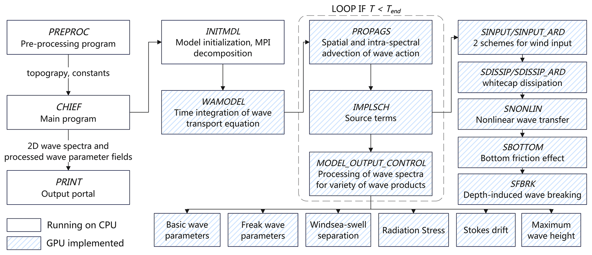
Figure 1 Flow diagram of WAM6 for a regular wave modeling. WAM6 modeling is implemented with a three-step procedure, including pre-processing (PREPROC), model integration (CHIEF), and output (PRINT). The shaded box denotes the computing-intensive modules that are ported to the GPU.

3 Porting WAM6 to a GPU

Before porting a complex code package to GPU, the developers should consider whether the core algorithm is suitable for the GPU (applicability), whether the programming effort is acceptable (programmability), whether the ported code can fit the rapidly evolving and diverse hardware (portability), and whether it can scale efficiently to multiple devices (scalability). CUDA and OpenACC are two commonly used GPU programming tools. CUDA can access all features of the GPU hardware to enable more optimization. A number of studies on GPU-accelerated hydrodynamic models have been reported to use CUDA C or CUDA Fortran as coding languages (Xu et al., 2015; de la Asunción and Castro, 2017; Qin et al., 2019; Yuan et al., 2020). Substantial efforts have to be done to encapsulate the computing code with CUDA kernels. However, a lesson learned by us is that using CUDA to rewrite a code package which is under community development is not always a smart choice. OpenACC is a parallel programming model which provides a collection of instructive directives to offload computing code to GPUs and other multi-core CPUs. Using OpenACC greatly shortens the development time, reduces the learning curve of a non-GPU programmer, and supports multiple hardware architectures. Therefore, we adopted OpenACC as the coding tool.

To fully accelerate the WAM6 model and improve performance, the best practice is to offload all computing-intensive code to GPU devices and maximize data locality by keeping necessary data resident on GPU. The spectral wave model is memory-consuming due to the existence of 4D prognostic variable N (Eq. 1). For example, for a global $\mathrm{1}/\mathrm{10}$° wave model consisting of 36 directions and 35 frequencies, the variable of spectral wave energy is as large as 36 Gigabytes (GB). All coding strategies should comply with the facts that GPU memory is limited and data transfer between the host and device is expensive. As shown in Fig. 1, the overall strategy in this study is to run the entire CHIEF program on GPUs without any data transfer between CPU and GPU memories. For multiple-GPU programming, the CUDA-aware OpenMPI is used to conduct inter-GPU communication.

3.1 Data hierarchy

Unlike its predecessor, WAM6 is now modernized by the FORTRAN 90 standard. All subroutines are organized as groups and then encapsulated as modules in accordance with their purposes. As the spatial and intra-spectrum resolutions increase, the memory usage for global wave modeling shows exponential growth. Hence, careful design of the data structure and exclusion of unnecessary variables on the GPU, which require a panorama of the entire WAM6 model as well as a thorough analysis of individual variables, are important.

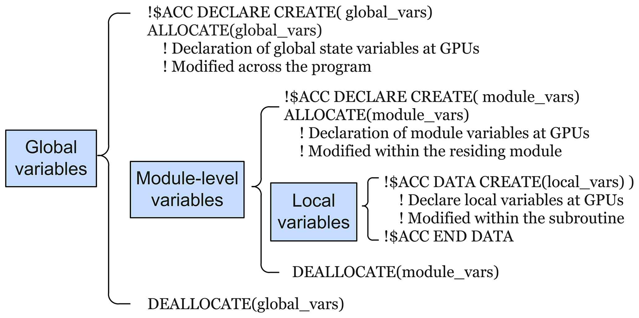
As illustrated in Fig. 2, a three-level data hierarchy is established, with each level having a different lifetime and scope. The prognostic and state variables are constantly modified during the program runtime and declared as global variables using the 〈acc declare〉 directive with the create clause. The module-level variables are private to the module where they are declared. They have the same lifetime of the residing module and are also defined on the GPU using the 〈acc declare〉 directive. For the global and module-level variables, the FORTRAN allocate statement allocates the variables to both host and device memories simultaneously. The OpenACC uses the 〈acc data〉 directive to create local variables that are only accessible locally inside a subroutine. They are allocated and freed within the 〈acc data〉 region.

Figure 2 The three-level data hierarchy of WAM6-GPU v1.0.

3.2 Optimization strategies

OpenACC implementation can literally be as simple as inserting directives before specific code sections to engage the GPUs. However, to fully utilize the GPU resource, optimizations such as code refactoring or even algorithm replacing, which require a wealth of knowledge of both GPU architecture and code package itself, are necessary. Before introducing the optimizing strategies, some knowledge about WAM6, especially that related to GPU computing, is reiterated here.

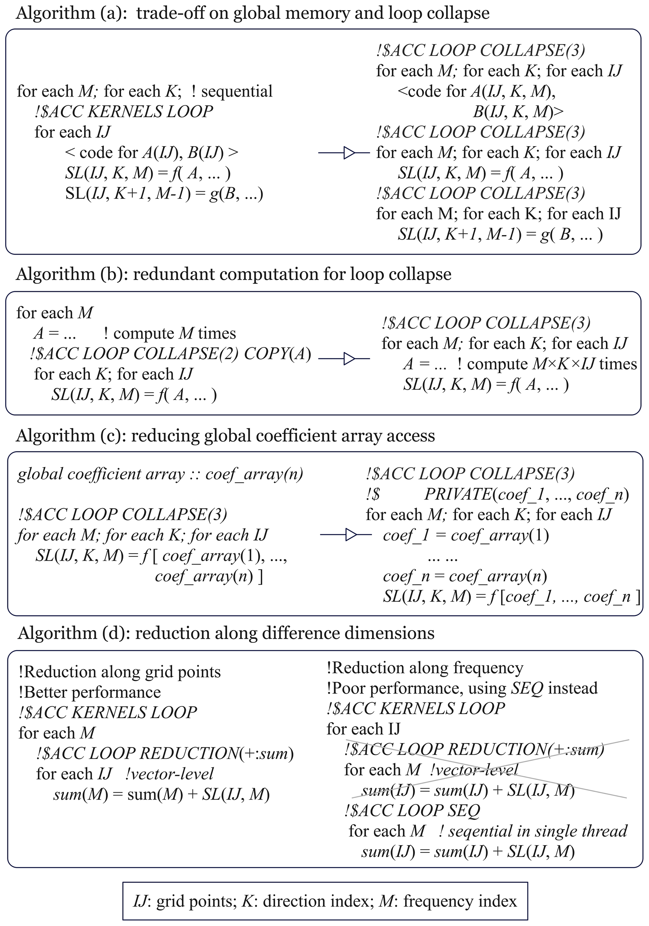
Figure 3 Optimizing strategies to improve performance in WAM6-GPU v1.0. In the model, the three-level nested loops are extremely common and IJ, M, and K denote indexes of the grid cell, frequency, and direction.

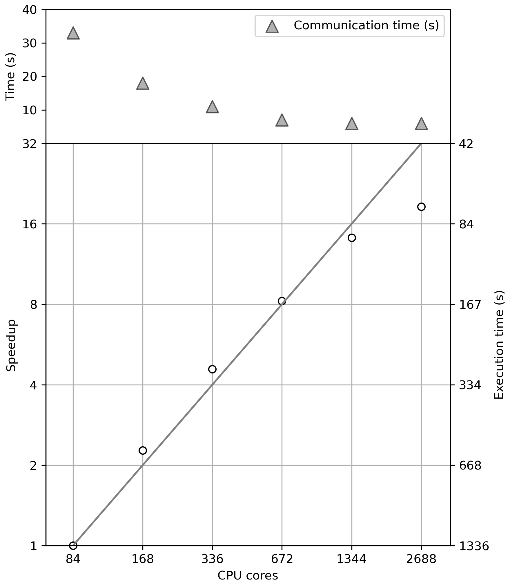
Figure 4 MPI scalability of WAM6 for a global 0.1° 1 d wave hindcast case (T1) on NMEFC's HPC cluster with Intel Xeon E5-2680 v4 processors. The diagonal line denotes linear scalability. Both speedup (left y axis) and corresponding execution time in seconds (right y axis) are shown by open cycles.

First of all, WAM6 is computing-intensive, so GPU accelerating is certainly promising. A global $\mathrm{1}/\mathrm{10}$° high-resolution wave modeling (corresponding to nearly 3 million grid points) with 35 frequencies and 36 directions means that approximately 4 billion equations have to be solved in a single time step. In WAM6, a mapping from the 2D spherical grid to a 1D array is performed. Thus, the computation of wave physics is mainly composed of a series of three-level nested loops iterating each grid, frequency and direction. Iteration on grid points is placed in the innermost loop for vectorization where appropriate. Nevertheless, as explained later, better performance sometimes requires a loop on grid points placed on the outermost level, leaving two other loop levels to execute serially.

Secondly, WAM6 can be memory- and input/output (I/O)-bound as it contains a dozen of 3D variables with overall size amounting to hundreds of Gigabytes. Some optimizing strategies, such as loop collapse, contain a tradeoff between performance and memory occupancy. Besides, previous work (Ikuyajolu et al., 2023) only accelerates source terms of the wave model, and post-processing of spectral wave energy for a variety of wave parameters has not been ported to GPUs. This leads to a mass device-to-host transfer of the 3D wave spectra at each output time step. The consequence is that the achieved speedup ratio is immediately neutralized by the transfers.

Thirdly, the nonlinear wave–wave interaction (S_nl) redistributes energy over wave components with similar frequencies and directions. Thus, parallelism along the dimensions of frequency and direction cannot be performed. Optimizing strategies on S_nl should be considered carefully. Spectral separation of wind sea and swell also involves manipulation between of wave components which cannot be vectorized either.

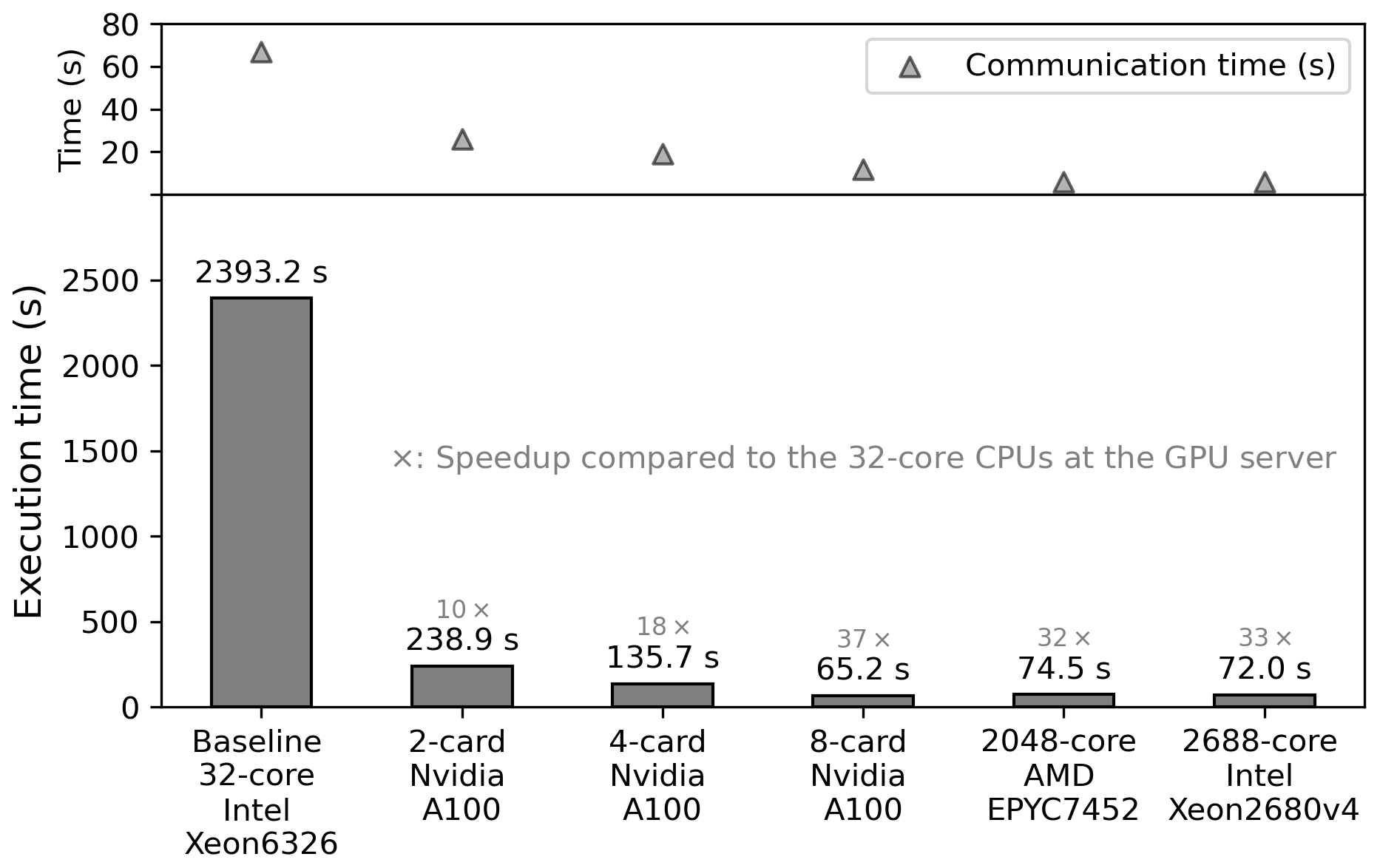
Figure 5 Speedup ratios of WAM6-GPU v1.0 on two, four, and eight NVIDIA A100 cards over its original code on a 32-core node with two Intel Xeon 6326 processors for a 1 d global 0.1° wave hindcast. The computing time of the CPU code on the NMEFC and BJSC's HPC clusters is also included. Speedup ratios are labeled over the bars. MPI communication time is denoted as solid triangles.

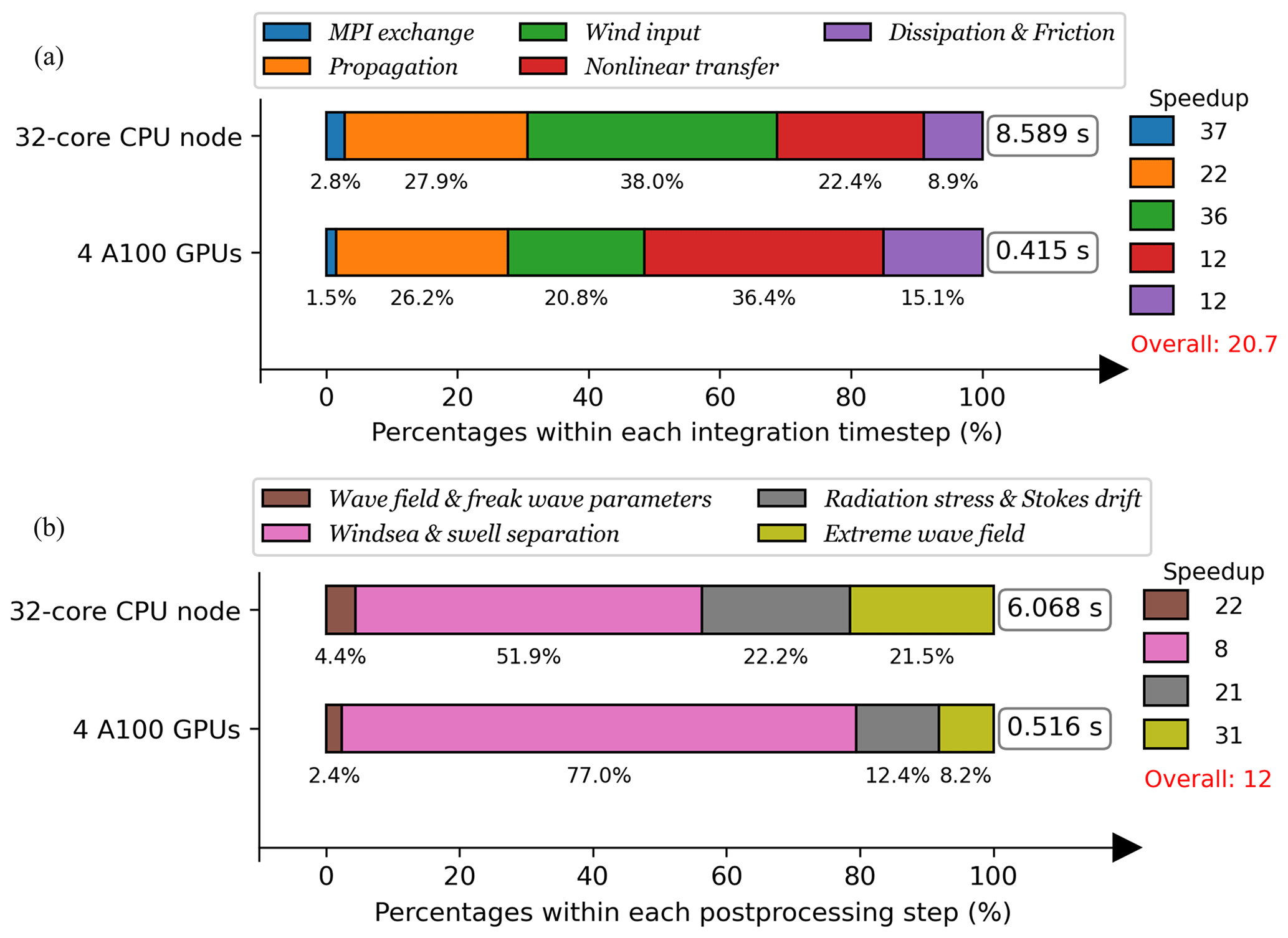
Figure 6 GPU runtime analysis within the integration (a) and post-processing (b) time steps for a global 0.1° wave hindcast case.

Generally, we pursue a high GPU occupancy by loop reordering, collapse, and refactoring. The key principles are to tune how the loops are mapped to the GPU hardware and allocate optimal workload and on-chip resources for each CUDA core. We take full advantage of on-chip memories and caches by evaluating the necessity of each global memory access and whether it can be converted to on-chip access. We completely eliminate device-host memory copies during the runtime of the program by migrating the whole wave physics and post-processing modules to the GPUs. It should be noted that too much code refactoring may be detrimental to code readability in terms of its physical concept. Based on the full absorption of model physics, loop reordering and collapse are the main strategies for better speedup and have not altered the code structure in most cases. Heavy code refactoring only occurs when computing the source term of nonlinear wave interactions as well as in some MPI interface functions. More specifically, some of the code optimization is presented by a few examples as follows:

• Restructuring the complex loops. The wave physics of WAM6 consists of complex loops with nested functions and a number of private scalars or local variables. The simplest implementation is to insert OpenACC directives before the outer loops to generate huge GPU kernels and using 〈acc routine〉 to automatically parallelize the nested functions. The implementation does work but comes with poor performance generally. A GPU kernel of appropriate size helps to achieve better performance. When appropriate, we split complex loops into a series of short and concise loops to increase parallelism and GPU occupancy. For nested subroutines, a naive usage of 〈acc routine〉 is not encouraged. A rule of thumb is to make a loop-level (fine-grained) parallelism inside the nested subroutines with a complex structure.

  Nevertheless, splitting the outermost loop into pieces sometimes leads to a dilemma. In WAM6, evaluation of the spectral wave energy is a 3D computation. As shown in Fig. 3a, local intermediate scalars or variables have to be declared as 3D variables to store the temporary information. It is commonplace in the subroutine to compute the nonlinear wave–wave interaction, S_nl. Although splitting the loop can achieve vectorization along all loop levels (right panel of Algorithm (a) in Fig. 3), the space of GPU memory may be limited in this case, not to mention the overhead for creating/freeing the memory each time. Thus, tradeoff between parallelism and global memory must be considered.

• Increasing parallelism by loop collapse. Except aforementioned loop splitting, loop reordering is commonly used to organize the nested loops. We ensure that the 3D global variables are being accessed consecutively along the dimensions in an increasing manner. OpenACC then collapses the nested loops into one dimension. For the nested loops without any dependency, we place the grid-cell-based loop (IJ) to the innermost level, which is immediately followed by the direction- (K) and frequency-based (M) loops. Loop collapse is limited to tightly nested loops. As shown in Fig. 3b, for loosely nested loops, some scalars are computed between the nested loops. If appropriate, these scalars are placed into the innermost loop at the cost of computing them redundantly. In this way, the loops are converted to the tightly nested loops.

• Reducing global memory allocation and access. Global memory allocation and access are expensive operations on GPU, which may incur performance degradation. One widely used strategy is to convert 2D or 3D local variables in the nested loops to loop-private scalars if appropriate. In the subroutine to evaluate S_nl, there are parameter arrays that store dozens of factors for spectral components of the wave. As exhibited in Fig. 3c, the best practice is to assign each value of the array to a temporary scalar which is private to the loop rather than to offload the array to the global memory of the device. The latter would substantially increase global memory access. Using too many private scalars inside one kernel raises the concerns of a possible lower GPU occupancy due to spills of registers. The fact is that OpenACC tries to handle it properly by manipulating the physical resource (i.e., registers and L1/L2 cache) for these local variables without degrading performance notably.

• Choosing longest dimension for reduction. Reduction operations are ubiquitous in WAM6. A simple usage of the 〈acc reduction〉 construct along the dimensions of frequency or direction should be avoided. It requires a parallel level of vector in OpenACC to do the reduction at each grid point, leaving the majority of threads idle. Instead, we should map each thread to a grid point and instruct the thread to do the reduction in a serial way (Fig. 3d). The approach can fully occupy the GPU resource. Using 〈acc reduction〉 for global reduction along the longest dimension, IJ, is encouraged.

  For multiple-GPU MPI communication, we fill the sending and receiving buffers by GPU and using the 〈acc host_data〉 construct for device-to-device data exchange. This dramatically reduces MPI communication time (Fig. 5).

4 Performance evaluation

4.1 Hardware and model configuration

WAM6-GPU v1.0 is tested on a GPU server with eight NVIDIA A100 GPUs. The compilation environment is NVIDIA HPC SDK version 22 and NetCDF v4.3. The NVIDIA A100 consists of 6912 CUDA cores sealed on 108 streaming multiprocessors. These cores access 80 GB of device memory in a coalesced way. The GPU server is hosted by two Intel Xeon 6236 CPUs with 32 (2 × 16) physical cores running at 2.9 GHz. In this study, the test case first runs on these two CPUs with 32 cores fully occupied, and the corresponding execution time (measured in second) is chosen as the baseline for speedup computation. Speedup ratio is defined as a ratio of the baseline time over the execution time of the same test case on GPUs.

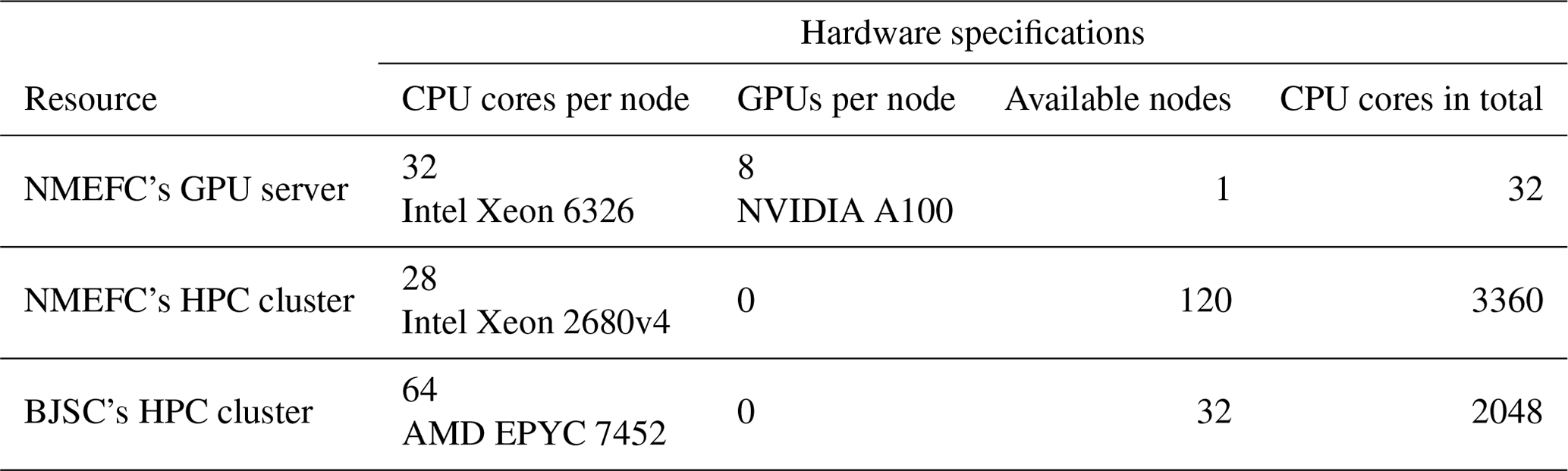
Furthermore, two HPC clusters are used to test the MPI scalability of WAM6. The National Marine Environmental Forecasting Center of China's (NMEFC's) cluster has 120 active computing nodes, and each of them has dual Intel Xeon E5-2680 v4 CPUs with 28 cores. The Beijing Super Cloud Computing Center's (BJSC's) cluster provides us with a 32-node computing resource. Each node has dual AMD EPYC 7452 CPUs with 64 cores. The hardware configurations are listed in Table 1.

Table 1 Hardware configurations for performance evaluation of WAM6-GPU v1.0.

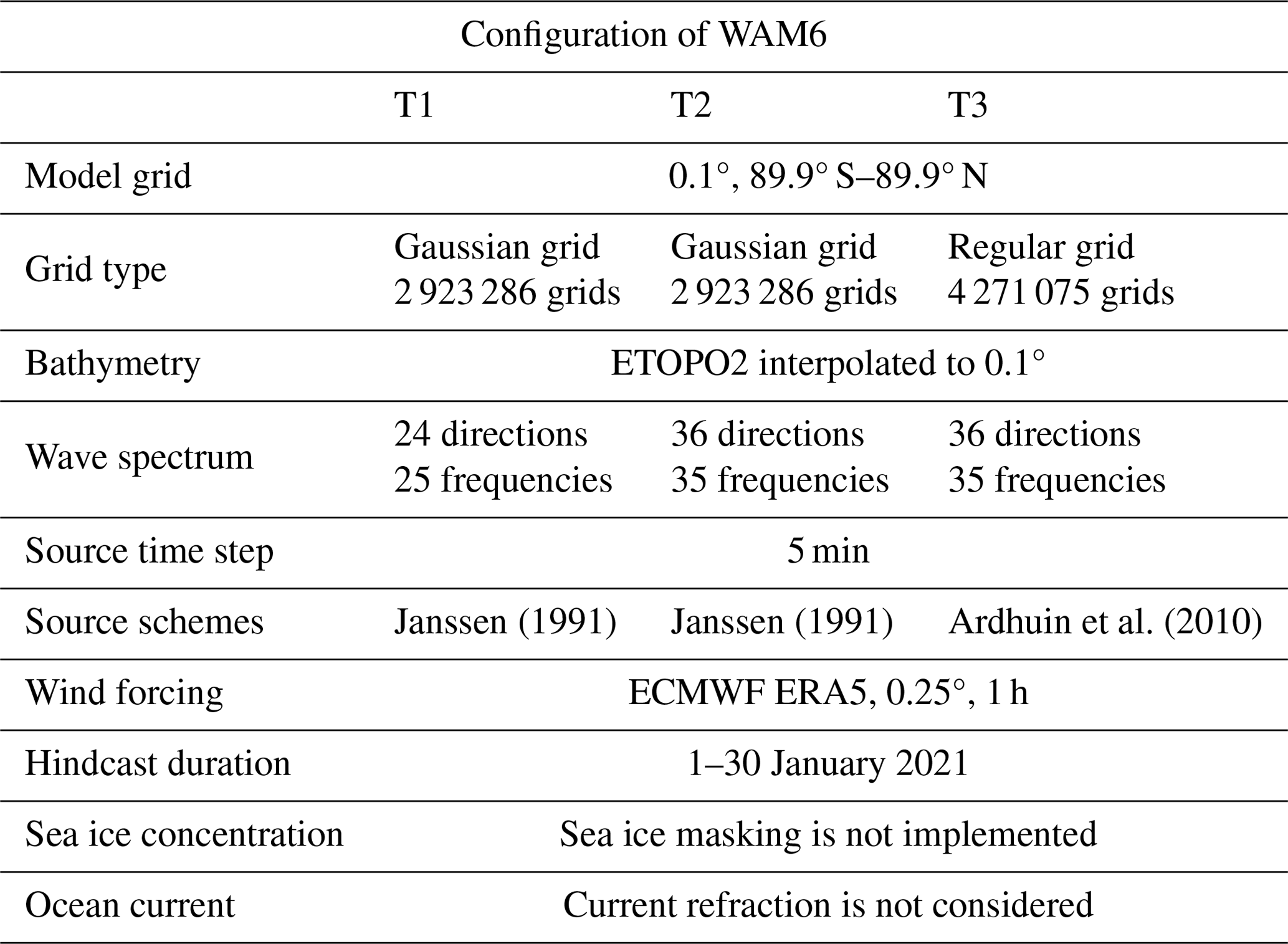
To evaluate the performance of WAM6-GPU v1.0, three test cases (hereafter referred as to T1–T3) are configured to conduct a global high-resolution wind hindcast. The model configuration is summarized in Table 2. In T1, the global model runs on a reduced Gaussian grid at a horizontal resolution of 0.1° and the wave spectrum at each grid point is discretized with 24 directions and 25 frequencies. The modeling area extends to a latitude of 89.9° in the Arctic and Antarctic regions. The total number of grid points is 2 923 286. The resolution of wave spectrum changes to 36 directions and 35 frequencies for T2. In T3, a regular grid is adopted and the number of grid points increases to 4 271 075. According to the CFL condition, the time step for propagation reduces from 43 to 0.9 s. In short, the computing workload gets heavier as the spectral resolution and grid points increase from T1 to T3. Generally, the regular grid adopted in T3 is not used for practical global modeling.

The hourly ECMWF ERA5 reanalysis (Hersbach et al., 2020) is used as atmospheric forcing with a spatial resolution of 0.25°. Output parameters are generated at an interval of 3 h. WAM6-GPU v1.0 is configured as a stand-alone model which does not consider sea ice–wave interaction and current refraction. Two schemes for wave growth and dissipation parameterization (Janssen, 1991; Ardhuin et al., 2010) are used with integrating time step of 5 min. The scheme of Ardhuin et al. (2010) is slightly more computing-intensive. In the study, the performance metric is based on the average computing time required for a 1 d global wave hindcast collected from 30 d simulations (1–30 January 2021).

Janssen (1991)Janssen (1991)Ardhuin et al. (2010)

Table 2 Summary of the configuration for the global wave hindcast cases.

4.2 Speedup comparisons

First of all, MPI scalability of WAM6 is evaluated on NMEFC's HPC cluster using 84, 168, 336, 672, 1344, and 2688 cores, respectively. The T1 case is used. As shown in Fig. 4, WAM6 exhibits perfect linear scaling up to 1344 cores. The drop in scalability becomes significant when the T1 case is split into 2688 cores. In this case, a 1 d global wave hindcast requires at least 72.0 s. The communication time for the exchange of the overlapping halo cells among the neighboring sub-domains (upper panel in Fig. 4) declines, and the curve gradually flattens, as was expected.

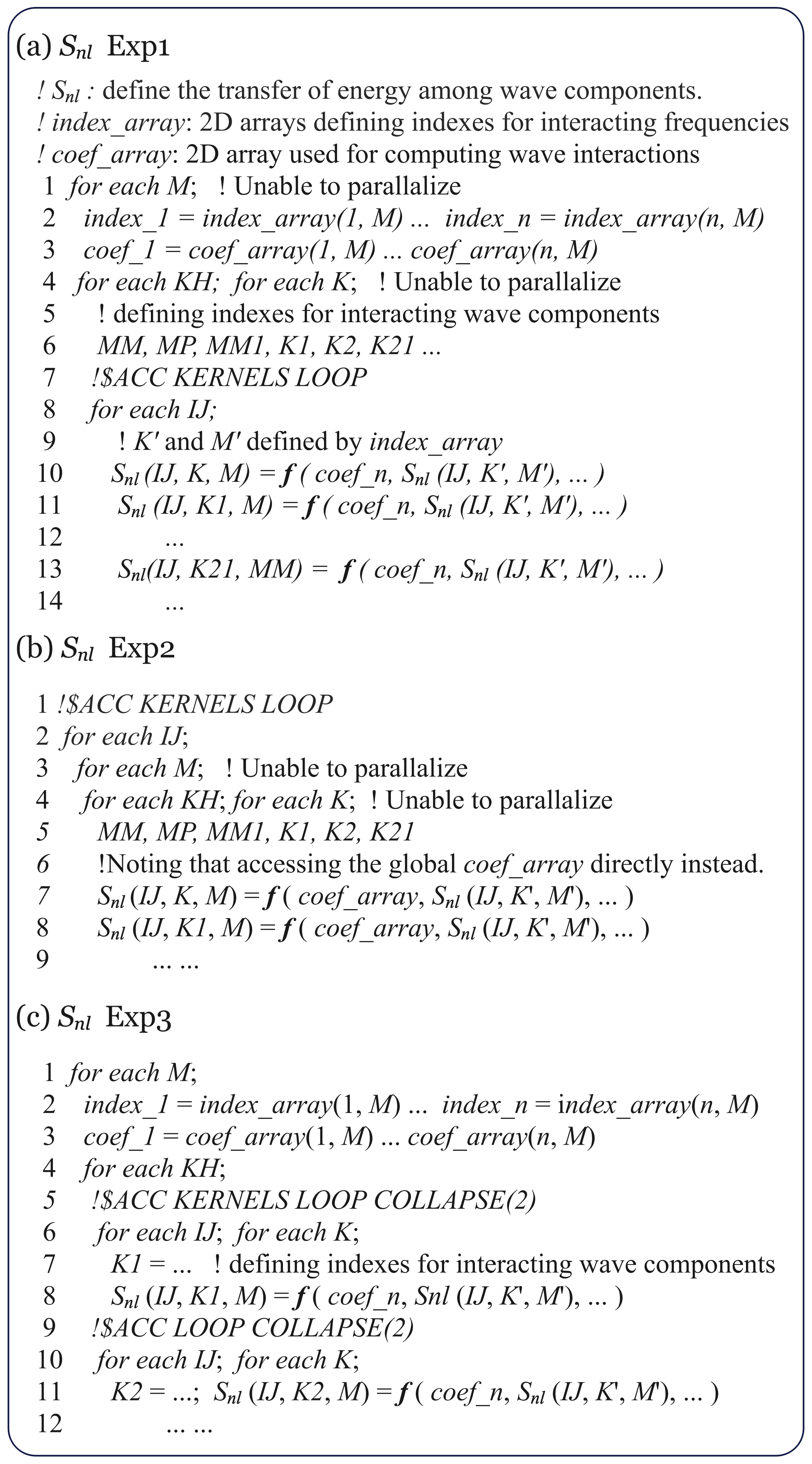
Figure 7 Pseudocode of optimizing experiments on the source term describing nonlinear wave interaction (S_nl). Algorithms in panels (a)–(c) correspond to Exp1–3 separately.

In Fig. 5, the bar plot displays the execution time and speedup ratios of WAM6-GPU v1.0 when allotted to a different hardware resource. The T1 case is used. The original code is first placed on NMEFC's GPU server with only 32 CPU cores fully used. The average wall time taken to run a 1 d forecast is 2393.2 s. Time necessary for model initialization is excluded. We then choose it as baseline to compute speedup ratios, which are annotated in gray text in Fig. 5.

Overall, when running on two GPUs, WAM6-GPU v1.0 can achieve a speedup of 10 over the dual-socket CPU node, and a near-linear scaling can be observed when four and eight GPUs are allocated. This means when the eight-card GPU server is at full strength, the maximum speedup ratio can achieve the value of 37, which greatly shortens the execution time of the 1 d global wave modeling to 65.2 s. As a comparison, the T1 case has been tested on the NMEFC's and BJSC's HPC clusters (Table 1). The execution times are 72.0 and 74.5 s separately when 2688 and 2048 cores are allocated to each cluster, corresponding to speedup ratios of 33 and 32. The GPU-accelerated WAM6 model shows its superiority over the original code with regard to computing efficiency. It should be noted that showcasing the performance of GPU acceleration over CPU is somewhat difficult. The reported speedup ratios vary in terms of the hardware and workload.

For an operational 7 d wave forecast, the global model usually adopts a reduced Gaussian grid and spectral resolution of 36 directions and 35 frequencies, which is similar to the T2 case in the study. Therefore, the energy consumption (E) of a 7 d global wind forecast using the T2 case is measured by $E=P_{\mathrm{chip}}\cdot N\cdot T$ in terms of the chip's thermal design power (TDP). P_chip is the TDP value of the GPU/CPU chip, N is the number of devices, and T is the computing time of the model. For the NVIDIA A100 GPU and Intel Xeon 2680v4 CPU, the TDP values are 350 and 120 W, respectively. In the NMEFC, the operational global wave model runs for 2.5 h on NMEFC's cluster (Table 1) with 560 cores. A global wave forecast consumes 0.84 kWh on the eight-card GPU server (Table 3) and approximately 12 kWh on NMEFC's cluster. That means at least 90 % of power could be saved if an eight-card GPU server is used.

Table 3 GPU memory and computing time required for a 7 d global 0.1° wave forecast on the GPU server^a.

^a The specification of the GPU server is presented in Table 1. ^b Model configurations are presented in Table 2.

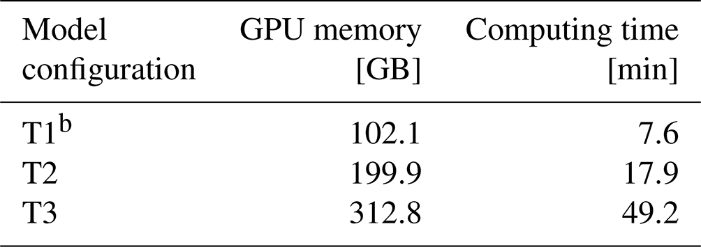
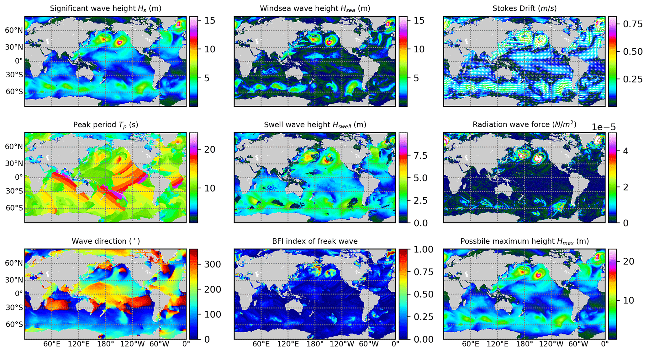
Figure 8 A series of output parameters generated by WAM6-GPU v1.0.

4.3 GPU profiling

The major processes of WAM6 and its GPU version are profiled, and their performance is illustrated by timeline plots in Fig. 6. WAM6 runs with two CPUs with 32 cores, and its GPU version runs with four GPUs. In the T1 case, the time intervals for wave propagation, source term integration, and wave parameter computation are 43 s, 5 min, and 3 h, respectively. The profiling of wave propagation and source term integration in a 5 min period is presented in Fig. 6a.

At each integration time step, the model begins with the MPI exchange of 3D spectral energy, which is followed by the computation of propagation and source terms. Generally, a complete model integration on CPUs takes 8.589 s, while its GPU counterpart takes only 0.435 s on four A100 cards. This corresponds to a speedup ratio of 20. In more detail, for the original CPU version, wave propagation and wind input (S_in) are 2 major computing-intensive processes, which contribute 27.9 % and 38.0 % of the runtime, respectively. For the GPU version, the most prominent feature is that the share of nonlinear transfer (S_nl) soars to 36.4 %. By adopting optimizing strategies introduced in Sect. 3.2, OpenACC implementation of wave propagation and S_in can take full advantage of GPU resources. On the contrary, the computation of S_nl requires five layers of loops, and the dependency along frequency and direction inhibits multi-level parallelism. The original algorithm only allows parallelization on the IJ loop. A naive implementation of OpenACC results in very poor performance and substantially lower speedup ratio. Extensive optimizing experiments on S_nl have been made to reduce its share from nearly 60 % to 36.4 %. Among these experiments, three of them (Exp1–3) are summarized below, with their time measurements shown in brackets. The pseudocode is shown in Fig. 7.

1. Exp1. Placing the IJ loop to the innermost level (not adopted; 0.214 s) leads to too much overhead for serially launching thousands of kernels in a single time step.

2. Exp2. Placing the IJ loop to the outermost level and accessing global coefficient and index arrays directly (not adopted; 0.252 s) leads to lower GPU occupancy and higher GPU latency due to spilling of local memory, and frequent access to these arrays within a kernel is detrimental to performance.

3. Exp3. Placing the IJ loop between the M (frequency) and K (direction) loops (adopted; 0.171 s for loop collapse on IJ and K and 0.151 s for parallelism on IJ and sequential execution on K) overcomes the shortcomings of the above experiments. Besides, two actual tests have been conducted in Exp3. By reorganizing the code substantially, we managed to collapse the IJ and K loops at first. As the second test, we did not perform the loop collapse and simply inserted 〈acc loop seq〉 before the nested K loop. Surprisingly, the second test took 0.02 s less. Although loop collapse on IJ and K may increase code parallelism, it seems that the reorganized code leads to increased overhead.

Furthermore, in contrast with the common sense that MPI exchange is a limiting factor for speedup, in this study, its GPU implementation exhibits a considerable speedup, with its share reducing from 2.8 % to 1.5 %. The best practice is to pack and decode the MPI buffers through GPU acceleration, and transfer them using the 〈acc host_data〉 construct.

WAM6 has several post-processing modules to derive a series of wave parameters from wave spectra at each output time step (ECMWF, 2023). Some of the derived parameters serve as interface variables for coupling with atmospheric, oceanic, and sea ice models (Breivik et al., 2015; Roberts et al., 2018). It is found that even though these modules are only used at each output time step (normally 1–3 h), the device-to-host transfer of the 3D spectral energy is so expensive that the overall performance can be affected. Besides, as shown in the timeline, the post-processing runs for 6.068 s on the CPU node. Considering the post-processing is both computing-intensive and I/O-bound, these modules are ported to the GPU in the study. The profiling of these modules is shown in Fig. 6b. The post-processing is categorized into four types shown in the figure legend. GPU implementation exhibits acceptable acceleration with a speedup metric of 12. As expected, the spectral separation takes the largest share of the runtime (77.0 %) as it involves a succession of frequency-dependent loops. Not much optimization has been done at this time.

4.4 Comparison of CPU and GPU results

The numerical models running on CPUs and GPUs are supposed to produce slightly different results due to multiple factors. For example, the execution order of the arithmetic operations are different on CPUs and GPUs for a global reduction. Besides, iterative algorithms lead to the accumulation of the errors. Substantive difference is not allowed, and ideally it should not grow rapidly for a long-term simulation. The absolute difference ($\mathrm{AD}=\mathrm{CPU}-\mathrm{GPU}$) and relative difference ($\mathrm{RD}=(\mathrm{CPU}-\mathrm{GPU})/\mathrm{CPU}$) are used to measure the difference between the CPU and GPU results. Both WAM6 and its GPU version run with single precision for a 1-month period.

As many as 72 different wave parameters can be computed by WAM6-GPU v1.0, and some of them are visualized in Fig. 8. The field-mean AD and RD values for a 1 d period are presented in Fig. 9 as gray cycles and open triangles, respectively. Generally, GPU implementation is proven to be a success, which is demonstrated by the well-controlled differences. The mean AD values are well below 10⁻⁶, with several outliers observed for some output parameters whose values are several orders of magnitude larger than those of others (i.e., radiation stress components and wave direction in degrees). In this case, the RD metric is more appropriate for comparison. Time series of mean relative differences (RDs) from 1 to 30 January 2021 for significant wave height, peak and mean wave period, and wave direction are shown in Fig. 10. Two dashed lines marking the RD value of 10⁻⁶ are plotted. The differences between CPU and GPU results do not show a growing trend for the whole simulation.

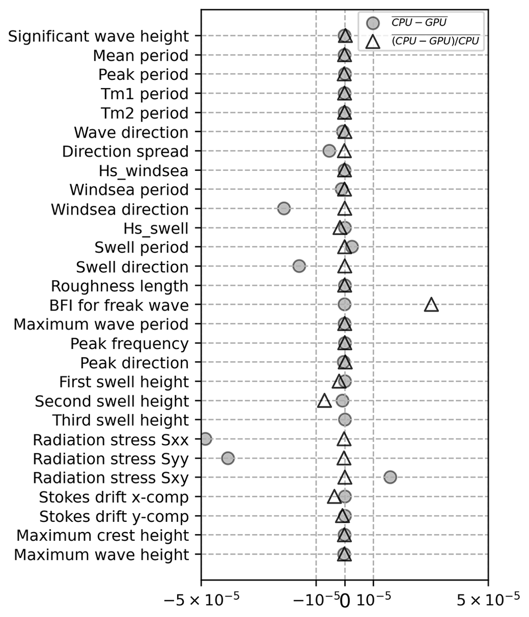
Figure 9 Mean difference (cycles) and mean relative differences (triangles) between WAM6 and WAM6-GPU v1.0 for major output parameters for a 1 d global simulation. Both versions use single precision for computation. Outliers in mean difference can be observed for parameters that are several orders of magnitude larger than others.

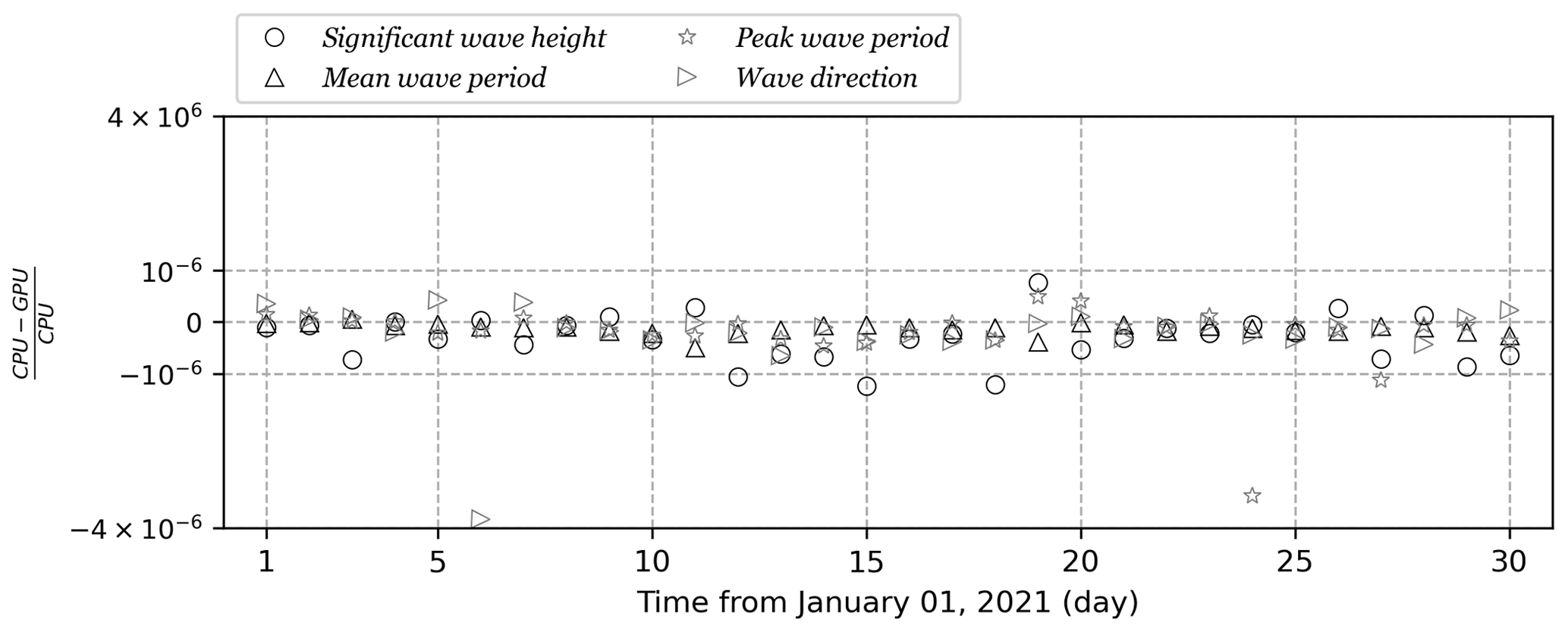
Figure 10 Time series of mean relative differences (RDs) between WAM6 and its GPU version from 1 to 30 January 2021 for significant wave height (circles), peak wave period (stars), mean wave period (triangle), and wave direction (right-pointing triangles).

5 Conclusions

In recent years, giant HPC clusters have been replaced by dense and green ones at an increasing pace. Moreover, programming barriers to porting numerical models to GPUs are now incredibly low with the aid of high-level programming tools such as OpenACC. These progresses pave a fast lane to energy-efficient computing for climate and Earth system modeling. It is anticipated that the transition of ESMs from CPU-based infrastructure to GPU-based computing devices is inevitable.

In this study, WAM6, one of the most commonly used spectral ocean wave models, has been ported to multiple GPUs by OpenACC with considerable efforts of code restructuring and refactoring. To evaluate model performance, a global wave hindcast case has been configured with a horizontal resolution of $\mathrm{1}/\mathrm{10}$° and intra-spectrum resolution of 25 × 24 or 35 × 36. It shows that when using an eight-card GPU server (NVIDIA A100), a speedup of 37 over a fully loaded CPU node can be achieved, which reduces the computing time of a 7 d global wave modeling from more than 2 h to 7.6 min. We expect an even higher performance of WAM6-GPU v1.0 on the latest NVIDIA H100 GPU. The study emphasizes that for a complicated model, GPU performance may not be desirable if OpenACC directives are implemented without substantial consideration of GPUs' features and their combination with code itself.

To move the study forward, the ongoing works include adding a new finite-volume propagation scheme to support a Voronoia unstructured grid, and incorporating sea ice–wave interaction source term to WAM6's physics. These works will extend the application of the code to the polar areas and nearshore.