Modelling chemical advection during magma ascent

Modelling magma transport requires robust numerical schemes for chemical advection. Current numerical schemes vary in their ability to be mass conservative, computationally efficient, and accurate. This study compares four of the most commonly used numerical schemes for advection: an upwind scheme, a weighted essentially non-oscillatory (WENO-5) scheme, a semi-Lagrangian (SL) scheme, and a marker-in-cell (MIC) method. The behaviour of these schemes is assessed using the passive advection of two different magmatic compositions. This is coupled in 2D with the temporal evolution of a melt anomaly that generates porosity waves. All algorithms, except the upwind scheme, are able to predict the melt composition with reasonable accuracy, but none of them is fully mass conservative. However, the WENO-5 scheme shows the best mass conservation. In terms of total running time and when multithreaded, the upwind, SL, and WENO-5 schemes show similar performance, while the MIC scheme is the slowest due to reseeding and removal of markers. The WENO-5 scheme has a reasonable total run time, has the best mass conservation, is easily parallelisable, and is therefore best suited for this problem.

1 Introduction

Mechanisms of magma ascent and emplacement within the lithosphere and upper asthenosphere remain largely unconstrained (e.g. Connolly and Podladchikov, 2007b; Katz et al., 2022). Studies have attempted to address this problem using techniques ranging from geophysical measurements of the present-day lithosphere to geochemical analysis of the rock record. However, geophysical studies are hampered by indirect measurements, and natural samples in geochemical studies represent only the end-product of the melting processes (Brown, 2013; Clemens et al., 2022; Johnson et al., 2021). Comparatively, numerical modelling allows the investigation of these processes at a range of scales in space and time (e.g. Keller, 2013; Katz and Weatherley, 2012).

To numerically model such open systems, it is necessary to be able to describe the chemical and physical processes responsible for magma ascent in a rock. At low melt fractions and in the absence of externally applied stress, the physical processes are based on the continuum formulation of two-phase flow. It takes into account the concurrent mechanisms of rock matrix compaction and buoyancy of partial melt in an interconnected porous network (e.g. Scott and Stevenson, 1984; McKenzie, 1984). This formulation is based on mass and momentum conservation and an appropriate set of constitutive relationships. In addition, conservation of energy needs to be ensured to link mechanical to chemical processes (e.g. Katz, 2008). Chemical processes, such as phase reactions, can be considered using thermodynamics and/or kinetics and relate the equilibration of the melt with the hosting rock (e.g. Omlin et al., 2017; Bessat et al., 2022). They contribute to the transport dynamics by changing rock properties, such as density, viscosity, porosity, and permeability (Jha et al., 1994; Aharonov et al., 1995b; Keller and Katz, 2016). However, the amount of melt interacting with the rock is also modulated by transport mechanisms (Kelemen et al., 1997; Spiegelman and Kenyon, 1992; Aharonov et al., 1995a). Therefore, the development of integrated models that successfully describe the complex interaction between reaction and transport is key to understanding melting and melt extraction at all scales.

Numerous numerical studies have investigated reactive melt transport. It has been shown that melts that partially crystallise or dissolve the host rock could be a viable mechanism for channelling flow and creating heterogeneities in the mantle in the context of mid-ocean ridges (Aharonov et al., 1997; Spiegelman et al., 2001) and sub-arc magmatism (Bouilhol et al., 2011). Concerning lower-crust melting, this approach has mainly been used to understand the processes of chemical differentiation and the compositional range of magmas in mafic systems (e.g. Jackson et al., 2005; Solano et al., 2012; Riel et al., 2019).

One challenge of reactive melt transport modelling is the advection of the melt composition through its ascent. This part, which is mathematically well understood, being described by a mass balance equation, is numerically challenging (e.g. LeVeque, 1992). This is mainly due to the fact that most numerical models are based on a Eulerian frame of reference, where the discretised space is fixed in space and in time. In contrast, transport is by essence better defined from a Lagrangian perspective, where the observer follows the particles of fluid as they move. In addition, two-phase flow models are at least 2D problems due to the formation of channels (e.g. Barcilon and Lovera, 1989; Connolly and Podladchikov, 2007b) and to the fact that mass cannot be transported efficiently in 1D in the melt (Jordan et al., 2018). This brings a limitation to the resolution of the models and hence requires accurate advection schemes.

This study compares four numerical schemes applied to the problem of the advection of magmatic composition: an upwind scheme, a weighted essentially non-oscillatory (WENO) scheme, a semi-Lagrangian (SL) scheme, and a marker-in-cell (MIC) method. This selection provides a representation of the different approaches to solving advection problems that are commonly used in a wide range of applications. We assess the performance of each scheme in terms of accuracy, mass conservation, and computational time. A 2D model coupling chemical advection with a two-phase flow solver is then used to evaluate which algorithm is best suited for this problem.

2 Governing equations

Chemical transport in two-phase flow systems is described by the four mass conservation equations of the system (e.g. Aharonov et al., 1997). The first two equations describe the conservation of the total mass of the solid and the liquid:

$$\begin{array}{}\text{(1)}& {\displaystyle \frac{\partial \left[(\mathrm{1}-\mathit{\varphi }){\mathit{\rho }}_{\mathrm{s}}\right]}{\partial t}}=-\mathrm{\nabla }\cdot \left[(\mathrm{1}-\mathit{\varphi }){\mathit{v}}_{\mathbf{s}}{\mathit{\rho }}_{\mathrm{s}}\right],\text{(2)}& {\displaystyle \frac{\partial \left(\mathit{\varphi }{\mathit{\rho }}_{\mathrm{f}}\right)}{\partial t}}=-\mathrm{\nabla }\cdot \left(\mathit{\varphi }{\mathit{v}}_{\mathrm{f}}{\mathit{\rho }}_{\mathrm{f}}\right),\end{array}$$

where f and s represent the fluid and solid phases, t is the time (in s), ϕ is the fluid-filled porosity, ρ is the density of the respective phase (kg s⁻³), and v is the velocity of the respective phase (m s⁻¹). The last two equations express the conservation of each chemical component within the solid and fluid phases:

$$\begin{array}{}\text{(3)}& {\displaystyle }\begin{array}{rl}{\displaystyle \frac{\partial \left[(\mathrm{1}-\mathit{\varphi }){\mathit{\rho }}_{\mathrm{s}}{C}_e^{\mathrm{s}}\right]}{\partial t}}& =\mathrm{\nabla }\cdot \left[D_e^{\mathrm{s}}(\mathrm{1}-\mathit{\varphi }){\mathit{\rho }}_{\mathrm{s}}\mathrm{\nabla }{C}_e^{\mathrm{s}}\right.\\ & \left.-(\mathrm{1}-\mathit{\varphi }){\mathit{v}}_{\mathbf{s}}{\mathit{\rho }}_{\mathrm{s}}{C}_e^{\mathrm{s}}\right],\end{array}\text{(4)}& {\displaystyle \frac{\partial \left(\mathit{\varphi }{\mathit{\rho }}_{\mathrm{f}}{C}_e^{\mathrm{f}}\right)}{\partial t}}=\mathrm{\nabla }\cdot \left({\mathit{D}}_e^{\mathrm{f}}\mathit{\varphi }{\mathit{\rho }}_{\mathrm{f}}\mathrm{\nabla }{C}_e^{\mathrm{f}}-\mathit{\varphi }{\mathit{v}}_{\mathrm{f}}{\mathit{\rho }}_{\mathrm{f}}{C}_e^{\mathrm{f}}\right),\end{array}$$

where C_e is the mass fraction of the chemical component e in the respective phase, $D_e^{\mathrm{s}}$ is the solid diffusion coefficient of the chemical component e (in m² s⁻¹), and ${\mathit{D}}_e^{\mathrm{f}}$ is the hydrodynamic dispersion tensor of the chemical component e in the fluid (m² s⁻¹). These four equations assume no mass transfer due to reactions between the solid and the liquid phases.

Simplifications

In this study, the advection of the chemical components transported by the liquid phase is considered, and the diffusion term in Eqs. (3) and (4) is neglected. Since ρ_s is assumed to be constant and the host rock has a fixed composition, Eq. (3) is omitted.

Subtracting Eq. (2) in Eq. (4), and dividing by ρ_f and ϕ yields

$$\begin{array}{}\text{(5)}& {\displaystyle \frac{\partial C_e^{\mathrm{f}}}{\partial t}}=-{\mathit{v}}_{\mathrm{f}}\mathrm{\nabla }\cdot C_e^{\mathrm{f}}.\end{array}$$

Equation (5) is formally equivalent to Eq. (4) without the dispersion term. Moreover, Eq. (4) is written in conservative form, whereas Eq. (5) is expressed in Lagrangian or non-conservative form. Equation (5) removes the time dependence on ϕ and is linear. It is a common form used in the reactive transport modelling community (e.g. Carrera et al., 2022).

An expression for v_f can be derived by coupling Eqs. (1) and (2) to the momentum conservation equations (e.g. McKenzie, 1984; Bercovici et al., 2001). These are usually solved before Eq. (5); a description of the system used in this study is provided below in Sect. 5.1.

3 Numerical methods

Solving an advection equation using a linear Eulerian scheme leads to high numerical diffusion for first-order schemes, such as the upwind scheme (Courant et al., 1952), and to oscillations on sharp gradients for higher-order schemes (LeVeque, 2002). The latter effect is described by Godunov's theorem (Godunov and Bohachevsky, 1959). This theorem states that linear Eulerian schemes with an order of accuracy greater than 1 cannot preserve the monotonicity of the solution for sharp gradients, discontinuities, or shocks. This has led to extensive developments in the design of high-order Eulerian non-linear schemes that can achieve high accuracy without bringing oscillations. Examples of such developments are the essentially non-oscillatory (ENO) methods (Harten et al., 1987) that later led to WENO schemes (Liu et al., 1994). These schemes are based on the idea of using a non-linear adaptive procedure to automatically choose the locally smoothest stencil, and early examples of applications include the modelling of shocks appearing in acoustics (e.g. Grasso and Pirozzoli, 2000) or solving the Hamilton–Jacobi equations (e.g. Jiang and Peng, 2000).

Another approach is to use schemes closer to the Lagrangian perspective, such as the MIC (or alternatively named marker-and-cell) method (e.g. Harlow et al., 1955; Gerya and Yuen, 2003a). It consists of tracking individual particles on a Lagrangian frame and reinterpolating them when needed on a Eulerian stationary grid. This approach has the advantage of producing little numerical diffusion, being unconditionally stable, and has been extensively used in geodynamic models (e.g. Gerya, 2019; van Keken et al., 1997; Duretz et al., 2011).

Finally, there are intermediate methods, such as semi-Lagrangian methods, trying to take advantages from both Eulerian and Lagrangian schemes (Robert, 1981; McDonald, 1984). These schemes look at different particles at each time step, considering only particles whose final trajectories correspond to the position of grid nodes. This has the advantage of only considering a number of particles equal to the resolution of the Eulerian grid and is computationally efficient. They are also unconditionally stable but have issues with mass conservation (Chandrasekar, 2022). They were first developed for atmospheric modelling (e.g. Robert, 1981; Staniforth and Côté, 1991) and later successfully used in the plasma modelling community (e.g. Sonnendrücker et al., 1999).

To solve for Eq. (5) in the context of two-phase flow, we implemented and tested four different advection schemes that are representative of the approaches described above: an upwind scheme, a WENO scheme, an SL scheme, and a MIC method.

3.1 Upwind scheme

The upwind scheme is among the simplest algorithms for solving an advection equation on a Eulerian grid (e.g. LeVeque, 1992). It is explicit and first order in space and in time. It consists of using a spatially biased stencil that depends on the direction of the flow (Fig. 1).

3.1.1 Spatial discretisation

Using a first-order spatially biased stencil, Eq. (5) can be approximated for one chemical element and in 1D as

$$\begin{array}{}\text{(6)}& \begin{array}{rl}{\displaystyle \frac{\partial C_i}{\partial t}}& +v_{\mathrm{f},i}{\displaystyle \frac{C_i^n-C_{i-\mathrm{1}}^n}{\mathrm{\Delta }x}}=\mathrm{0}\text{for}{v}_{\mathrm{f},i}>\mathrm{0},\\ {\displaystyle \frac{\partial C_i}{\partial t}}& +v_{\mathrm{f},i}{\displaystyle \frac{C_{i+\mathrm{1}}^n-C_i^n}{\mathrm{\Delta }x}}=\mathrm{0}\text{for}{v}_{\mathrm{f},i}<\mathrm{0},\end{array}\end{array}$$

where i is a spatial index in the x direction, Δx is the constant grid spacing, and v_f,i is the x component of the fluid velocity.

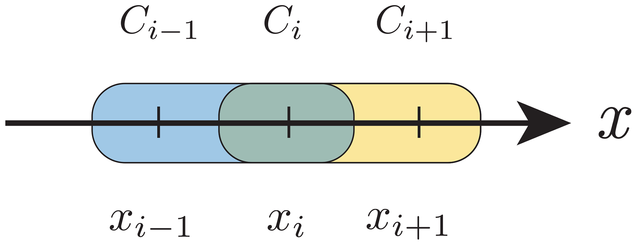
Figure 1 Spatial stencil of the upwind scheme in 1D. The blue box is the valid stencil for positive velocities and the yellow box for negative velocities.

3.1.2 Temporal discretisation

Combined with the first-order forward Euler method, we retrieve the classical upwind scheme from Eq. (6):

$$\begin{array}{}\text{(7)}& \begin{array}{rl}{\displaystyle \frac{C_i^{n+\mathrm{1}}-C_i^n}{\mathrm{\Delta }t}}& +v_{\mathrm{f},i}{\displaystyle \frac{C_i^n-C_{i-\mathrm{1}}^n}{\mathrm{\Delta }x}}=\mathrm{0}\text{for}{v}_{\mathrm{f},i}>\mathrm{0},\\ {\displaystyle \frac{C_i^{n+\mathrm{1}}-C_i^n}{\mathrm{\Delta }t}}& +v_{\mathrm{f},i}{\displaystyle \frac{C_{i+\mathrm{1}}^n-C_i^n}{\mathrm{\Delta }x}}=\mathrm{0}\text{for}{v}_{\mathrm{f},i}<\mathrm{0},\end{array}\end{array}$$

where Δt is the time step.

It can also be rewritten in a more compact form:

$$\begin{array}{}\text{(8)}& C_i^{n+\mathrm{1}}=C_i^n-\mathrm{\Delta }t\left[v_{\mathrm{f},i}^{+}\left({\displaystyle \frac{C_i^n-C_{i-\mathrm{1}}^n}{\mathrm{\Delta }x}}\right)+v_{\mathrm{f},i}^{-}\left({\displaystyle \frac{C_{i+\mathrm{1}}^n-C_i^n}{\mathrm{\Delta }x}}\right)\right],\end{array}$$

where

$$\begin{array}{rl}{v}_{\mathrm{f},i}^{+}& =\text{max}(v_{\mathrm{f},i},\mathrm{0}),\\ v_{\mathrm{f},i}^{-}& =\text{min}(v_{\mathrm{f},i},\mathrm{0}).\end{array}$$

This scheme is well-known to produce a lot of numerical diffusion and is bounded by the following Courant–Friedrichs–Lewy (CFL) condition for p dimensions:

$$\mathrm{\Delta }t\left(\sum _{j=\mathrm{1}}^p{\displaystyle \frac{\left|v_{{\mathrm{f}}_j}\right|}{\mathrm{\Delta }{x}_j}}\right)\le {\mathit{Co}}_{\max }=\mathrm{1},$$

where Co_max is the maximum Courant (Co) number (e.g. Hirsch, 2007). In addition, it is not mass conservative for non-constant v_f, especially for divergent flow.

3.2 Weighted essentially non-oscillatory scheme

Weighted essentially non-oscillatory schemes were developed by Liu et al. (1994). The reader can refer to Shu (2009) for a comprehensive review of the development of WENO schemes and Pawar and San (2019) for implementations using Julia.

They are high-order schemes able to resolve sharp gradients, produce little numerical diffusion, but also follow the same CFL condition as the upwind scheme. The key idea behind them is to use a non-linear adaptive procedure to automatically choose the locally smoothest stencil. This allows WENO schemes to dispose of oscillations when advecting sharp gradients.

We use a fifth-order-in-space finite-difference approach for non-conservative problems, referenced as WENO-5 hereafter.

3.2.1 Spatial discretisation

Equation (5) can be discretised in space using the WENO-5 scheme similarly to the upwind scheme, in 1D, for one chemical element and for a single grid point such as

$$\begin{array}{}\text{(9)}& \begin{array}{rl}{\displaystyle \frac{\partial C_i}{\partial t}}& +v_{f,i}^{+}\left({\displaystyle \frac{C_{i+\frac{\mathrm{1}}{\mathrm{2}}}^L-C_{i-\frac{\mathrm{1}}{\mathrm{2}}}^L}{\mathrm{\Delta }x}}\right)\\ & +v_{f,i}^{-}\left({\displaystyle \frac{C_{i+\frac{\mathrm{1}}{\mathrm{2}}}^R-C_{i-\frac{\mathrm{1}}{\mathrm{2}}}^R}{\mathrm{\Delta }x}}\right)=\mathrm{0},\end{array}\end{array}$$

where

$$\begin{array}{rl}{C}_{i+\frac{\mathrm{1}}{\mathrm{2}}}^L& =w_{\mathrm{0}}^L\left({\displaystyle \frac{\mathrm{1}}{\mathrm{3}}}{C}_{i-\mathrm{2}}-{\displaystyle \frac{\mathrm{7}}{\mathrm{6}}}{C}_{i-\mathrm{1}}+{\displaystyle \frac{\mathrm{11}}{\mathrm{6}}}{C}_i\right)\\ & +w_{\mathrm{1}}^L\left(-{\displaystyle \frac{\mathrm{1}}{\mathrm{6}}}{C}_{i-\mathrm{1}}+{\displaystyle \frac{\mathrm{5}}{\mathrm{6}}}{C}_i+{\displaystyle \frac{\mathrm{1}}{\mathrm{3}}}{C}_{i+\mathrm{1}}\right)\\ & +w_{\mathrm{2}}^L\left({\displaystyle \frac{\mathrm{1}}{\mathrm{3}}}{C}_i+{\displaystyle \frac{\mathrm{5}}{\mathrm{6}}}{C}_{i+\mathrm{1}}-{\displaystyle \frac{\mathrm{1}}{\mathrm{6}}}{C}_{i+\mathrm{2}}\right),\\ C_{i-\frac{\mathrm{1}}{\mathrm{2}}}^R& =w_{\mathrm{0}}^R\left(-{\displaystyle \frac{\mathrm{1}}{\mathrm{6}}}{C}_{i-\mathrm{2}}+{\displaystyle \frac{\mathrm{5}}{\mathrm{6}}}{C}_{i-\mathrm{1}}+{\displaystyle \frac{\mathrm{1}}{\mathrm{3}}}{C}_i\right)\\ & +w_{\mathrm{1}}^R\left({\displaystyle \frac{\mathrm{1}}{\mathrm{3}}}{C}_{i-\mathrm{1}}+{\displaystyle \frac{\mathrm{5}}{\mathrm{6}}}{C}_i-{\displaystyle \frac{\mathrm{1}}{\mathrm{6}}}{C}_{i+\mathrm{1}}\right)\\ & +w_{\mathrm{2}}^R\left({\displaystyle \frac{\mathrm{11}}{\mathrm{6}}}{C}_i-{\displaystyle \frac{\mathrm{7}}{\mathrm{6}}}{C}_{i+\mathrm{1}}+{\displaystyle \frac{\mathrm{1}}{\mathrm{3}}}{C}_{i+\mathrm{2}}\right).\end{array}$$

Here, $C_{i-\frac{\mathrm{1}}{\mathrm{2}}}^L$ and $C_{i+\frac{\mathrm{1}}{\mathrm{2}}}^R$ are omitted to avoid redundancy. They can be obtained by shifting the index by −1 and 1, respectively.

The non-linear weights w are defined as

$$\begin{array}{rl}{w}_k^L& ={\displaystyle \frac{{\mathit{\alpha }}_k}{{\mathit{\alpha }}_{\mathrm{0}}+{\mathit{\alpha }}_{\mathrm{1}}+{\mathit{\alpha }}_{\mathrm{2}}}},{\mathit{\alpha }}_k={\displaystyle \frac{d_k^L}{{\left({\mathit{\beta }}_k+\mathit{ϵ}\right)}^{\mathrm{2}}}},k=\mathrm{0},\mathrm{1},\mathrm{2},\\ w_k^R& ={\displaystyle \frac{{\mathit{\alpha }}_k}{{\mathit{\alpha }}_{\mathrm{0}}+{\mathit{\alpha }}_{\mathrm{1}}+{\mathit{\alpha }}_{\mathrm{2}}}},{\mathit{\alpha }}_k={\displaystyle \frac{d_k^R}{{\left({\mathit{\beta }}_k+\mathit{ϵ}\right)}^{\mathrm{2}}}},k=\mathrm{0},\mathrm{1},\mathrm{2}.\end{array}$$

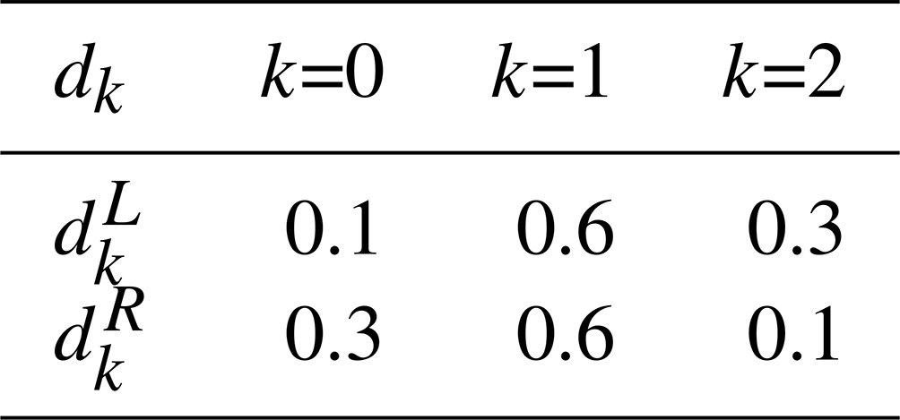
The values of the optimal weights $d_k^L$ and $d_k^R$ are given in Table 1. ϵ represents the machine epsilon, the relative approximation error due to rounding in floating-point arithmetic, and is used to avoid division by zero.

Table 1 Optimal weights for WENO-5 scheme.

Smoothness indicators β are equal to

$$\begin{array}{rl}{\mathit{\beta }}_{\mathrm{0}}& ={\displaystyle \frac{\mathrm{13}}{\mathrm{12}}}{\left(C_{i-\mathrm{2}}-\mathrm{2}{C}_{i-\mathrm{1}}+C_i\right)}^{\mathrm{2}}+{\displaystyle \frac{\mathrm{1}}{\mathrm{4}}}{\left(C_{i-\mathrm{2}}-\mathrm{4}{C}_{i-\mathrm{1}}+\mathrm{3}{C}_i\right)}^{\mathrm{2}},\\ {\mathit{\beta }}_{\mathrm{1}}& ={\displaystyle \frac{\mathrm{13}}{\mathrm{12}}}{\left(C_{i-\mathrm{1}}-\mathrm{2}{C}_i+C_{i+\mathrm{1}}\right)}^{\mathrm{2}}+{\displaystyle \frac{\mathrm{1}}{\mathrm{4}}}{\left(C_{i-\mathrm{1}}-C_{i+\mathrm{1}}\right)}^{\mathrm{2}},\\ {\mathit{\beta }}_{\mathrm{2}}& ={\displaystyle \frac{\mathrm{13}}{\mathrm{12}}}{\left(C_i-\mathrm{2}{C}_{i+\mathrm{1}}+C_{i+\mathrm{2}}\right)}^{\mathrm{2}}+{\displaystyle \frac{\mathrm{1}}{\mathrm{4}}}{\left(\mathrm{3}{C}_i-\mathrm{4}{C}_{i+\mathrm{1}}+\mathrm{3}{C}_{i+\mathrm{2}}\right)}^{\mathrm{2}}.\end{array}$$

The WENO-5 scheme requires, in 1D, a stencil of five points biased towards the left for positive velocities and five points biased towards the right for negative velocities as shown in Fig. 2. This commonly requires two ghost points on each side of the model to apply the boundary conditions. To extend this scheme to 2D, two new terms can be added to Eq. (9) for the new positive and negative component of v_f. The expressions of C at half points of the new index can be derived using the same formulae as in 1D for the new direction.

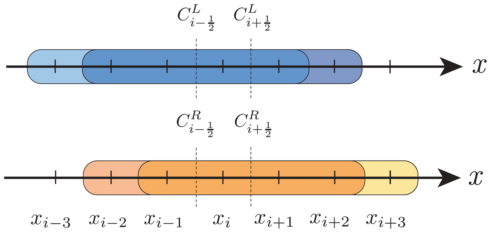
Figure 2 Spatial stencil of the WENO-5 scheme in 1D. C^L is used for positive velocities and C^R for negative velocities. The blue boxes are valid stencils for positive velocities, and the yellow and orange boxes are valid for negative velocities.

3.2.2 Temporal discretisation

Weighted essentially non-oscillatory schemes are not stable using the standard forward Euler time integration method (Wang and Spiteri, 2007). The most commonly used discretisation is the third-order strong stability preserving (SSP) explicit Runge–Kutta method (e.g. Jiang and Shu, 1996; Ghosh and Baeder, 2012). Strong stability preserving schemes are used to fully capture discontinuous solutions and are therefore well-suited for solving hyperbolic partial differential equations (Gottlieb et al., 2001).

The third-order SSP Runge–Kutta for Eq. (5) for one chemical element can be written as

$$\begin{array}{rl}{C}_i^{\mathrm{1}}& =C_i^n-\mathrm{\Delta }tL\left(C_i^n\right),\\ C_i^{\mathrm{2}}& ={\displaystyle \frac{\mathrm{3}}{\mathrm{4}}}{C}_i^n+{\displaystyle \frac{\mathrm{1}}{\mathrm{4}}}\left[C_i^{\mathrm{1}}-\mathrm{\Delta }tL\left(C_i^{\mathrm{1}}\right)\right],\\ C_i^{n+\mathrm{1}}& ={\displaystyle \frac{\mathrm{1}}{\mathrm{3}}}{C}_i^n+{\displaystyle \frac{\mathrm{2}}{\mathrm{3}}}\left[C_i^{\mathrm{2}}-\mathrm{\Delta }tL\left(C_i^{\mathrm{2}}\right)\right],\end{array}$$

with L being the spatial discretisation operator:

$$L\left(C_i\right)=v_{\mathrm{f},i}^{+}\left({\displaystyle \frac{C_{i+\frac{\mathrm{1}}{\mathrm{2}}}^L-C_{i-\frac{\mathrm{1}}{\mathrm{2}}}^L}{\mathrm{\Delta }x}}\right)+v_{\mathrm{f},i}^{-}\left({\displaystyle \frac{C_{i+\frac{\mathrm{1}}{\mathrm{2}}}^R-C_{i-\frac{\mathrm{1}}{\mathrm{2}}}^R}{\mathrm{\Delta }x}}\right).$$

With this formulation, the WENO-5 scheme is fifth order in space and third order in time.

3.3 Semi-Lagrangian schemes

Semi-Lagrangian schemes take a different approach than classical Eulerian methods and are related to tracer-based advection schemes. Semi-Lagrangian schemes aim to use the best of Lagrangian and Eulerian methods by solving the problem for particles whose trajectories pass through a fixed grid at the end of each time step rather than recording the full history of individual particles. They are therefore unconditionally stable. Two steps are usually required to implement SL schemes: trajectory tracing and interpolation back to the grid. In this study, a backward-in-time SL scheme is used for the trajectory tracing and the quasi-monotone scheme developed by Bermejo and Staniforth (1992) for the interpolation.

3.3.1 Trajectory tracing

The advantage of backward-in-time SL schemes is that the interpolant is defined from the Eulerian grid. In the case of a regular grid, this reduces the complexity of the implementation and the numerical cost of the interpolation function, since the interpolant is defined on a regular grid. From a particle point of view, the goal is to retrieve the position of the particle at time t_n for which the position corresponds to a grid point at time t_n+1. Using Eq. (5) for one chemical element and in 1D, the following ordinary differential equation has to be solved:

$$\begin{array}{}\text{(10)}& {\displaystyle \frac{\mathrm{d}x}{\mathrm{d}t}}={\mathit{v}}_{\mathrm{f}}(x,t).\end{array}$$

Knowing $x\left(t_{n+\mathrm{1}}\right)=x_i$, where i is a grid point, x(t_n)=x_d, where d is a departure point that needs to be found. In most practical cases, the velocity field varies greatly in time and in space between each time step, especially for porosity waves, so it is not easy to determine x_d. A common approach to accurately determine x_d is to use a linear multistep method such as the implicit mid-point scheme (Robert, 1981):

$$\begin{array}{}\text{(11)}& {\displaystyle \frac{x_i-x_d}{\mathrm{\Delta }t}}={\mathit{v}}_{\mathrm{f}}\left({\displaystyle \frac{x_i+x_d}{\mathrm{2}}},t_{n+\frac{\mathrm{1}}{\mathrm{2}}}\right),\end{array}$$

where v_f at time t_n+½ is obtained by taking the mean between the velocity at n and n+1. The assumption behind the mid-point rule is that the velocity remains constant at the mid-point value during each time step. This ensures that each trajectory is linear, with the mid-point being the average of the positions of its endpoints (Fig. 3). This method is a second-order accurate trajectory method in both space and time.

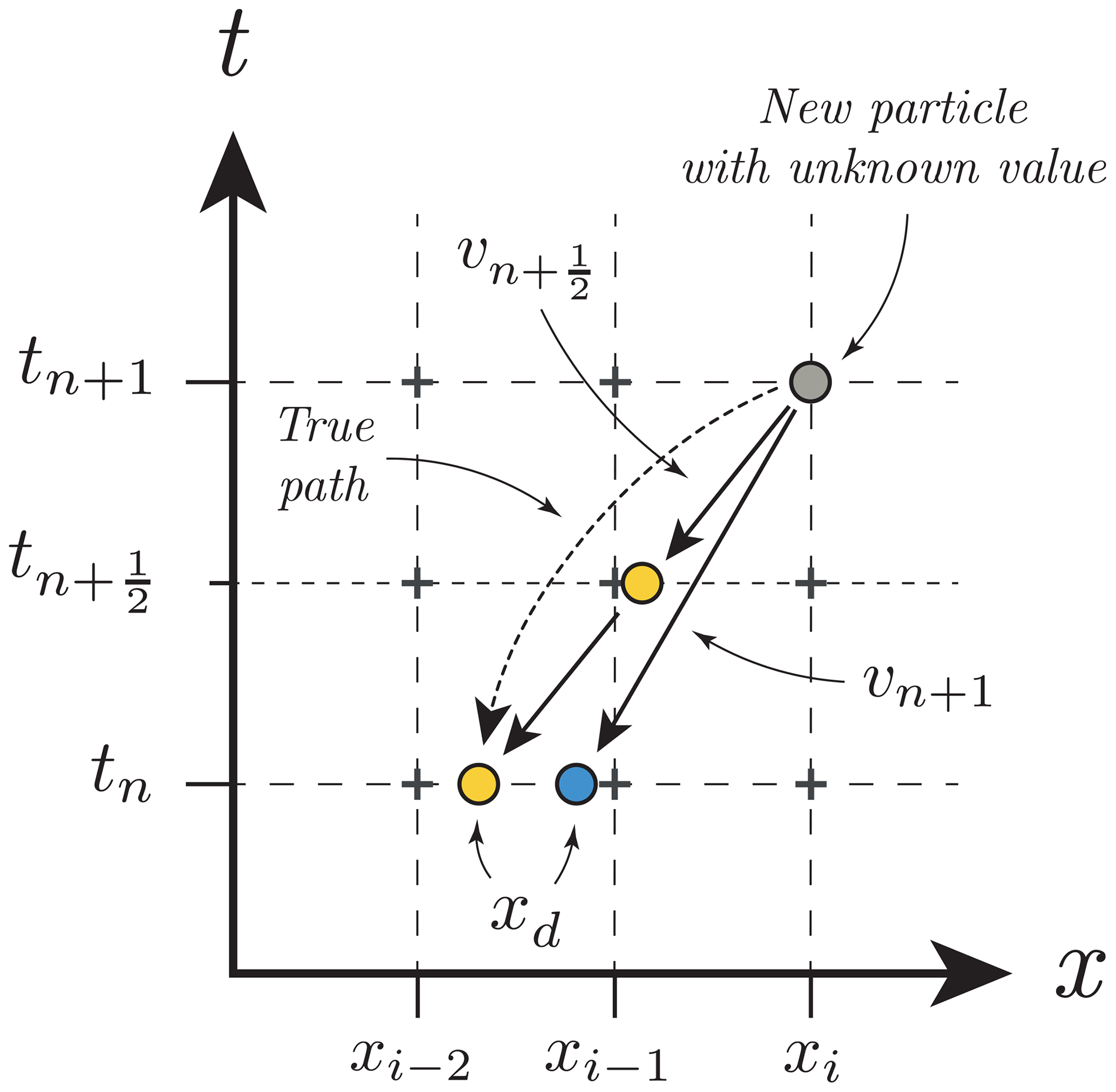
Figure 3 Summary of trajectory tracing for backward semi-Lagrangian schemes. The aim is to find the value of the advected quantity at the position x_i and at the time step t_n+1. The blue particle uses the velocity at n+1. The yellow particle shows the mid-point method, using an approximation of the velocity at $n+\frac{\mathrm{1}}{\mathrm{2}}$. The value of the particle at position x_d can then be interpolated at t_n to obtain the value at x_i at t_n+1.

Equation (11) must be solved implicitly because x_d is present on both sides of the equation and therefore requires iterations. It can be achieved for r iterations in this form:

$$\begin{array}{}\text{(12)}& x_d^{r+\mathrm{1}}=x_i-\mathrm{\Delta }t{\mathit{v}}_{\mathrm{f}}\left({\displaystyle \frac{x_i+x_d^r}{\mathrm{2}}},t_{n+\frac{\mathrm{1}}{\mathrm{2}}}\right).\end{array}$$

A minimum of three iterations while using linear interpolation has been shown to be sufficient in most cases (e.g. McDonald, 1984).

3.3.2 Interpolation

In most cases, x_d does not correspond to a grid node (see Fig. 3). In this case, interpolation is required to retrieve the value of the unknown at x_d:

$$C(x_d,t)=\mathcal{L}\left[C\left(x_{i_k}\right),t\right],$$

where ℒ is an interpolation operator and $x_{i_k}$ represents the nodes of the cell containing x_d.

Commonly, cubic interpolants are used as they offer a good compromise between performance and accuracy (e.g. Chandrasekar, 2022) and require in 1D four grid points $x_{i_k}$ per particle. Cubic B-splines are used in this study. Godunov's theorem still applies to linear SL schemes, and since cubic interpolation is third order in space, it introduces oscillations and overshoots for high gradients. To overcome this limitation, quasi-monotone (QM) SL schemes were developed by Bermejo and Staniforth (1992). The term QM means that the scalar field values cannot exceed the range of the previous time step but can still develop wiggles inside that range. Quasi-monotonicity is equivalent to the notion of being essentially non-oscillatory (Bermejo, 2001). A disadvantage of this method is an increased numerical diffusion, especially for a high Co number. A maximum Co number of 1.5 is generally used (e.g. Smith, 2000).

To implement quasi-monotone semi-Lagrangian (QMSL) schemes, let us define C⁻ and C⁺ as the minimum and maximum scalar values of the nodes of the cell containing x_d and C^H as the high-order non-monotone interpolant, here a cubic spline. Then, a local clipping can be applied at the end of each time step:

$$\begin{array}{}\text{(13)}& C^M\left(x_d,t\right)=\left\{\begin{array}{ll}{C}^{+}(x_d,t)& \text{if}{C}^H(x_d,t)>C^{+}(x_d,t),\\ C^{-}(x_d,t)& \text{if}{C}^H(x_d,t)<C^{-}(x_d,t),\\ C^H(x_d,t)& \text{otherwise},\end{array}\right.\end{array}$$

where C^M is the quasi-monotone interpolant. Equation (13) can be rewritten in a more compact way:

$$C^M\left(x_d,t\right)=\min \left\{\max \left[C^{-}\left(x_d,t\right),C^H\left(x_d,t\right)\right],C^{+}(x_d,t)\right\}.$$

Formally, this formulation is equivalent to a linear combination between a high-order interpolant and a first-order (monotone) interpolant (Bermejo, 2001).

3.4 Marker-in-cell schemes

Marker-in-cell schemes share the same ambition as SL schemes, such as being unconditionally stable, but are closer to Lagrangian schemes. They record the complete history of individual particles, called markers and interpolate their values on a fixed grid. This approach has the advantage of greatly reducing numerical diffusion and making MIC schemes unconditionally stable. In addition to trajectory tracing and interpolation, the MIC schemes require markers to be generated within the domain of the model.

3.4.1 Initial marker generation and reseeding of particles

The number of markers per cell required can vary depending on the complexity of the problem, here 5 markers per cell dimension and effectively 25 in 2D. This is generally sufficient to achieve good accuracy (e.g. Gerya, 2019). The initial value in each marker can then be directly derived from the initial conditions or obtained by linear interpolation from the initial conditions of the Eulerian grid.

For highly divergent flows or sometimes strongly stretching flows, it is necessary to regenerate or remove markers during the simulation. For highly divergent flows, this is because particles will accumulate in zones with negative divergence values and create a gap in zones with positive divergence values. For highly stretching flow, increases or gaps in the density of the markers can be induced by preferential flow in a particular direction. For reseeding, a non-conservative strategy similar to Keller et al. (2013) is used. If the marker density per cell is less than 25 % of the initial density, new markers are generated and assigned the value of the nearest marker. The old markers are discarded after this step. For marker accumulation, the marker density cannot exceed twice the initial density. If it does, a quarter of the markers are discarded at random.

3.4.2 Trajectory tracing

The goal of trajectory tracing for MIC schemes is to determine the position of each marker at the next time step. The same equation as Eq. (10) is solved. However, compared to backward SL where the final position is known, the unknown in this case is the position of the arrival point at tⁿ⁺¹. Also, the common way to solve this equation for MIC schemes is not using a linear multistep method such as the implicit mid-point scheme but rather Runge–Kutta schemes (Gerya, 2019). Using a second-order Runge–Kutta scheme, it consists of four steps. Interpolating v_f at t_n at the departure point x_d of the markers, finding the position of the markers at t_n+½ using v_f at t_n, reinterpolating the velocity at this new position, and using this new velocity to compute the arrival point x_a of the markers at t_n+1 from t_n.

Since classical interpolants do not retain the physical properties of the velocity field, such as its divergence, a simple bilinear interpolation may lead to unphysical clustering of markers on the timescale of a numerical model. To address this issue, Pusok et al. (2017) explored different interpolants and showed the advantages of using the LinP interpolation scheme (Gerya, 2019). The LinP interpolation scheme is an empirical relationship that combines two linear interpolants defined at the sides and at the centre of each cell. It is defined as

$${\mathit{v}}_{\mathrm{f}}\left(x,t\right)=A\mathcal{L}\left[{\mathit{v}}_{\mathrm{f}}\left(x_{\mathrm{side}},t\right)\right]+(\mathrm{1}-A)\mathcal{L}\left[{\mathit{v}}_{\mathrm{f}}\left(x_{\mathrm{center}},t\right)\right],$$

with A a constant commonly equal to $\mathrm{2}/\mathrm{3}$, ℒ a linear interpolant, and x_side and x_center the position of the sides and centre of the cell containing the marker.

Using this definition, we can rewrite the four steps of the second-order Runge–Kutta scheme in mathematical notation with four equations:

$$\begin{array}{rl}{\mathit{v}}_{\mathrm{f}}\left(x_d,t_n\right)& =A\mathcal{L}\left[{\mathit{v}}_{\mathrm{f}}\left(x_{\mathrm{side}},t_n\right)\right]+(\mathrm{1}-A)\mathcal{L}\left[{\mathit{v}}_{\mathrm{f}}\left(x_{\mathrm{center}},t_n\right)\right],\\ x_h& =x_d+{\displaystyle \frac{\mathrm{1}}{\mathrm{2}}}\mathrm{\Delta }t{\mathit{v}}_{\mathrm{f}}\left(x_d,t_n\right),\\ {\mathit{v}}_{\mathrm{f}}\left(x_h,t_n\right)& =A\mathcal{L}\left[{\mathit{v}}_{\mathrm{f}}\left(x_{\mathrm{side}},t_n\right)\right]+(\mathrm{1}-A)\mathcal{L}\left[{\mathit{v}}_{\mathrm{f}}\left(x_{\mathrm{center}},t_n\right)\right],\\ x_a& =x_d+\mathrm{\Delta }t{\mathit{v}}_{\mathrm{f}}\left(x_h,t_n\right),\end{array}$$

with x_h the intermediate position of the marker. Solving these four equations successively to obtain a value for x_a with this method is second order in space but only first order in time, as only the velocity at t_n is used.

3.4.3 Interpolation

After calculating the position of the markers, it is necessary to interpolate back on the Eulerian grid and/or to update the values of the markers from the Eulerian grid depending on the problem being solved. The step of updating the markers is not described in detail here, as it is not used in this study, but involves a simple interpolant when a regular grid is used. This step is more complex for updating the advected field on the Eulerian grid because the markers are not uniformly distributed for a non-trivial velocity field. Therefore, contrary to SL schemes, interpolation is performed on an unstructured grid as it is based on the position of the markers. In most cases, linear interpolants are used because they prevent oscillations, and the marker densities are high enough to prevent numerical diffusion. In this study, a weighted-distance-averaging linear interpolant is used (Gerya, 2019):

$$\begin{array}{rl}w\left(x_m,t_{n+\mathrm{1}}\right)& =\mathrm{1}-{\displaystyle \frac{\mathrm{\Delta }{x}_m}{\mathrm{\Delta }x}},\\ C\left(x_i,t_{n+\mathrm{1}}\right)& ={\displaystyle \frac{\sum _{i=\mathrm{1}}^{m}C\left(x_m,t_{n+\mathrm{1}}\right)w\left(x_m,t_{n+\mathrm{1}}\right)}{\sum _{i=\mathrm{1}}^{m}w\left(x_m,t_{n+\mathrm{1}}\right)}},\end{array}$$

where x_m is the position of a marker m, Δx_m is the distance between a marker m and the grid point i, and w is the weight of a marker m. All markers found in the cells surrounding grid point i are used for interpolation, as in Gerya and Yuen (2003b). The relationship between the markers and the grid in 2D is summarised in Fig. 4. One disadvantage of this interpolant is that it is prone to race conditions in shared memory systems, as it involves two sums, which require the use of atomic operations to parallelise the implementation.

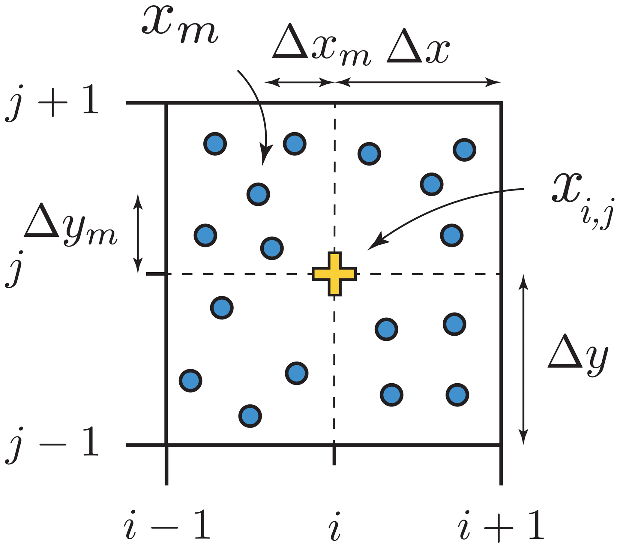
Figure 4 Sketch showing the geometric relationship in 2D between a point x_i,j of the Eulerian grid and the markers x_m used for the interpolation on a regular grid. The value at the point x_i,j is interpolated from the markers x_m contained inside the four neighbouring cells. x_i,j is fixed in time and in space, whereas the position of the markers x_m are time-dependent.

4 Numerical tests

To test the four advection schemes, two different numerical tests are performed in 2D: the pure rotation of a cylinder and the advection through a more complex velocity field mimicking a convection cell. In both cases, the domain is a square of size 1.0×1.0 with a constant spacing of $\mathrm{\Delta }x=\mathrm{\Delta }y=\mathrm{0.005}$ for a resolution of 201×201 nodes. The radius of the cylinder is 24Δx with a mass fraction of 1.0 and is centred at coordinates (0.25,0.25). The initial conditions for both tests are shown in Fig. 5.

For the first test, the time increment is Δt=400 with $\mathit{\omega }=\mathit{\pi }\times {\mathrm{10}}^{-\mathrm{5}}$, so it takes 500 time steps to make a full revolution. The velocity is defined as $\mathit{v}=(-\mathit{\omega }(y-\mathrm{0.5}),\mathit{\omega }(x-\mathrm{0.5}\left)\right)$, so the rotation is anti-clockwise, and the centre of it is at coordinates (0.5,0.5). The Co numbers inside the cylinder range between 0.45 and 0.8. The test is stopped after two revolutions. For the second test, v is defined as $\mathit{v}=(-\mathrm{2}\mathit{\pi }\times \sin (\mathit{\pi }x)\times \cos (\mathit{\pi }y),\mathrm{2}\mathit{\pi }\times \cos (\mathit{\pi }x)\times \sin (\mathit{\pi }y\left)\right)$. The time increment Δt is fixed by constraining the Co number to be 0.7 for a total time of 0.8 and 1016 time steps. At half of the total time, the opposite sign of v is taken as the new value of v, such that the analytical solution of the problem corresponds to the initial conditions.

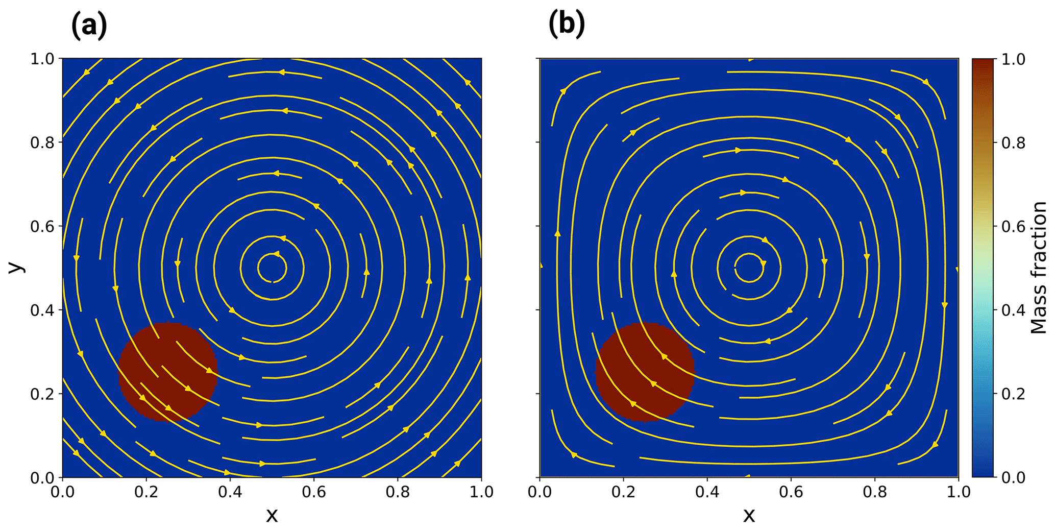
Figure 5 Initial conditions for the two numerical tests. The yellow arrows show the velocity fields of the tests. (a) Rotation of a cylinder. (b) Convection of a circular anomaly.

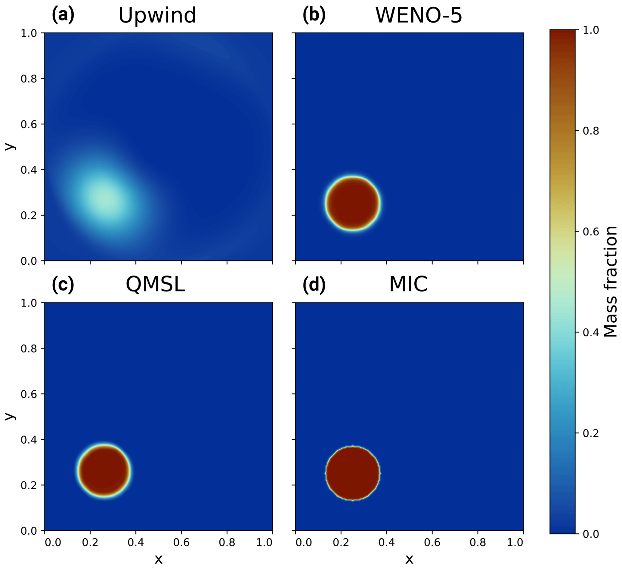
Figure 6 Results of the rotational test after two revolutions for the upwind, WENO-5, QMSL, and MIC schemes (a–d). Note that the upwind scheme was run with Δt=80 due to stability issues.

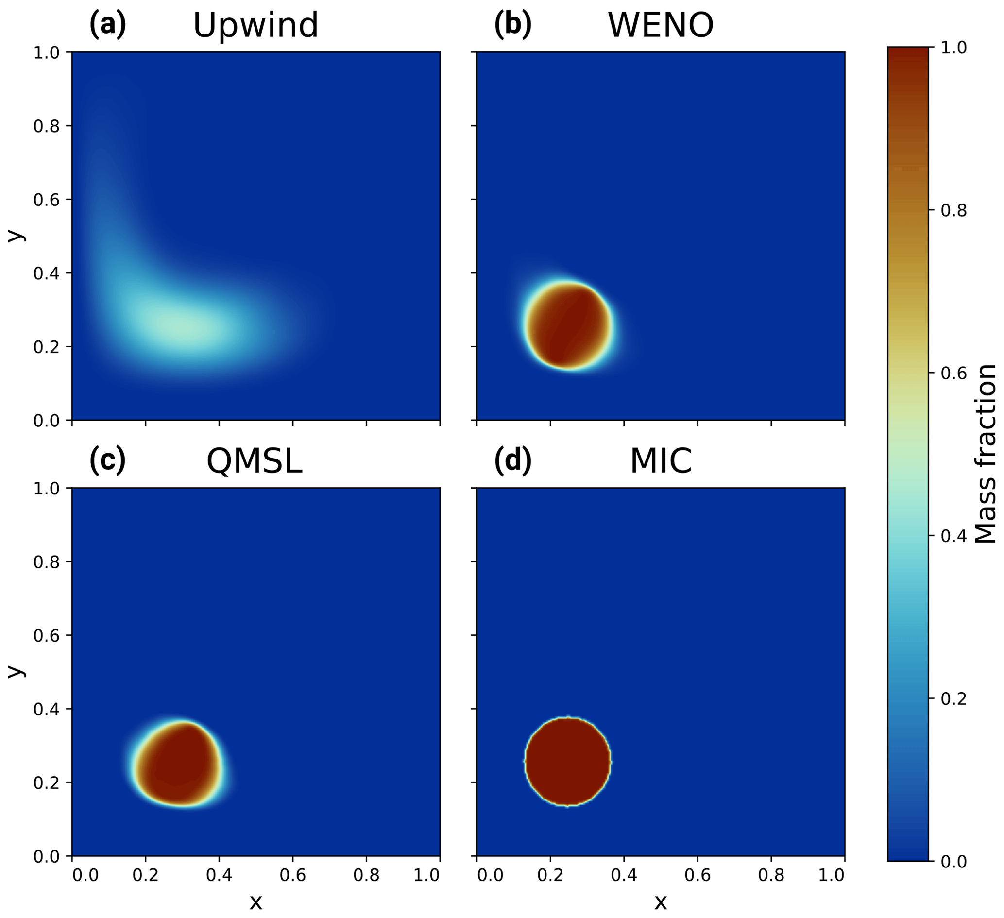
Figure 7 Results of the convection test after a total time of 0.8 for the upwind, WENO-5, QMSL, and MIC schemes (a–d). The velocity field was reversed at half of the total time so that the anomaly returns to its initial position.

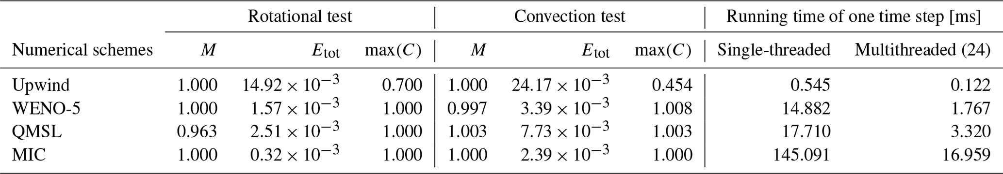
To compare and quantify the results of the different schemes, the following quantities were monitored: the mass conservation (M), the total error (E_tot), the maximum value of the final mass fraction (max(C_f)), and the minimum elapsed computational time of one time step after 10000 runs, with one thread and with 24 threads.

The mass conservation is defined as

$$\begin{array}{}\text{(14)}& M={\displaystyle \frac{\sum _{k=\mathrm{1}}^K\left(C_{\mathrm{f}}^k\right)}{\sum _{k=\mathrm{1}}^K\left(C_{\mathrm{0}}^k\right)}},\end{array}$$

where k is a 2D grid point index, K is the total number of grid points, $C_{\mathrm{f}}^k$ is the final mass fraction at index k, and $C_{\mathrm{0}}^k$ is the initial mass fraction at index k.

The total error in the scheme is defined as the mean square error:

$$E_{\mathrm{tot}}={\displaystyle \frac{\mathrm{1}}{K}}\sum _{k=\mathrm{1}}^K{\left(C_{\mathrm{0}}^k-C_{\mathrm{f}}^k\right)}^{\mathrm{2}}.$$

The results for both tests are reported in Table 2 and in Figs. 6 and 7 for the four different schemes. Both tests show the strong numerical diffusion of the upwind scheme and its high E_tot due to its first order in time and space. The WENO-5 scheme shows no oscillation and a good accuracy, being fifth order in space and third in time in both tests, with a small mass loss in the second test. The QMSL is not mass conservative for both problems. It shows a relatively good accuracy, being third order in space and second in time; is monotone; but shows deformation of the original cylinder at the end of the second test. Finally, for both tests, the MIC scheme is mass conservative and monotone and shows the best accuracy with almost no numerical diffusion. These simple tests highlight the properties of each scheme but use a velocity field that is divergence-free and without sharp variations. Coupling with a two-phase flow system is therefore necessary to assert which scheme is the more suitable in this case.

Table 2 Results of the two numerical tests for four advection schemes. The running time for the MIC does not include the reseeding and removal step of markers.

5 Coupling chemical advection and two-phase flow

Solving Eq. (5) for concrete cases implies having an expression for v_f at each time step. In this section, Eq. (5) is coupled to a transport model based on two-phase flow formalism. This transport model is used to model magma ascent in a porous solid phase. The main mechanism of transport is decompaction weakening, buoyancy, and failure and combines the formulations of Connolly and Podladchikov (2007a) and Vasilyev et al. (1998). It considers a compressible viscoelastic matrix with incompressible solid grains and an incompressible fluid phase, and it neglects the effect of shear stresses on fluid flow and compaction.

5.1 Two-phase flow formulation

In the case of a laminar fluid flow, conservation of momentum for the fluid can be expressed using Darcy's law:

$$\begin{array}{}\text{(15)}& \mathit{\varphi }({\mathit{v}}_{\mathrm{f}}-{\mathit{v}}_{\mathbf{s}})=-{\displaystyle \frac{k\left(\mathit{\varphi }\right)}{{\mathit{\mu }}_{\mathrm{f}}}}(\mathrm{\nabla }{P}_{\mathrm{f}}+{\mathit{\rho }}_{\mathrm{f}}\mathit{g}),\end{array}$$

with P_f the fluid pressure (in Pa), k the permeability (m²), a function of the filled porosity or melt fraction ϕ, μ_f the fluid viscosity (Pa s), and g the gravity vector (m s⁻²).

The relation between permeability and the filled porosity is assumed to follow the Kozeny–Carman law (Carman, 1939; Costa, 2006):

$$k=a{\mathit{\varphi }}^{\mathrm{3}},$$

where a is a proportionality constant.

The effective pressure P_e is defined as the difference between lithostatic pressure and fluid pressure:

$$\begin{array}{}\text{(16)}& P_{\mathrm{e}}=P_{\mathrm{lith}}-P_{\mathrm{f}},\end{array}$$

with P_lith the lithostatic pressure or the vertical load (in Pa). Substituting Eq. (16) in Eq. (15) and assuming constant rock density, we obtain

$$\begin{array}{}\text{(17)}& \mathit{\varphi }({\mathit{v}}_{\mathrm{f}}-{\mathit{v}}_{\mathbf{s}})={\displaystyle \frac{k\left(\mathit{\varphi }\right)}{{\mathit{\mu }}_{\mathrm{f}}}}\left(\mathrm{\nabla }{P}_{\mathrm{e}}+\mathrm{\Delta }\mathit{\rho }\mathit{g}\right).\end{array}$$

Considering the solid phase as a Maxwell body, we introduce rheology as the sum of viscous and poroelastic deformation:

$$\begin{array}{}\text{(18)}& \mathrm{\nabla }\cdot {\mathit{v}}_{\mathbf{s}}=-{\displaystyle \frac{P_{\mathrm{e}}}{\mathit{\zeta }(\mathit{\varphi },P_{\mathrm{e}})}}-{\mathit{\varphi }}^b{\mathit{\beta }}_{\mathit{\varphi }}{\displaystyle \frac{\partial P_{\mathrm{e}}}{\partial t}},\end{array}$$

where ζ is the volume viscosity of the rock (in Pa s), b a constant, and β_ϕ the pore compressibility modulus (Pa⁻¹). The terms on the right-hand side represent viscous and poroelastic deformation. Equation (18) is valid on the basis that shear stress is neglected.

The volume viscosity ζ is defined as a function of ϕ and P_e:

$$\mathit{\zeta }={\displaystyle \frac{{\mathit{\mu }}_{\mathrm{s}}}{{\mathit{\varphi }}^m}}\left[{\displaystyle \frac{\mathrm{1}}{R}}-H\left(P_{\mathrm{e}}\right)\left({\displaystyle \frac{\mathrm{1}}{R}}-\mathrm{1}\right)\right],$$

with μ_s the shear viscosity of the rock (in Pa s), m a constant, and R the decompaction weakening factor defined as the inverse of the R factor in Connolly and Podladchikov (2007a). H(P_e) is originally defined as the Heaviside function but is here approximated by a hyperbolic tangent function as similarly done by Räss et al. (2018).

We approximate here β_ϕ as the inverse of G, the shear modulus of the rock (in Pa):

$${\mathit{\beta }}_{\mathit{\varphi }}\approx {\displaystyle \frac{\mathrm{1}}{G}}.$$

This is valid for cylindrical pores, as described by Yarushina and Podladchikov (2015).

Summing up the right-hand sides of Eqs. (1) and (2) describing mass conservation and neglecting the change in densities, we obtain the total volumetric flux of material. Applying the divergence operator, we can derive

$$\begin{array}{}\text{(19)}& \mathrm{\nabla }\cdot \left[{\mathit{v}}_{\mathbf{s}}+\mathit{\varphi }({\mathit{v}}_{\mathrm{f}}-{\mathit{v}}_{\mathbf{s}})\right]=\mathrm{0}.\end{array}$$

We can then substitute Eqs. (17) and (18) in Eq. (19) to obtain

$$\begin{array}{}\text{(20)}& {\displaystyle \frac{P_{\mathrm{e}}}{\mathit{\zeta }(\mathit{\varphi },P_{\mathrm{e}})}}+{\displaystyle \frac{{\mathit{\varphi }}^b}{G}}{\displaystyle \frac{\partial P_{\mathrm{e}}}{\partial t}}=\mathrm{\nabla }\cdot \left[{\displaystyle \frac{k\left(\mathit{\varphi }\right)}{{\mathit{\mu }}_{\mathrm{f}}}}\left(\mathrm{\nabla }{P}_{\mathrm{e}}+\mathrm{\Delta }\mathit{\rho }\mathit{g}\right)\right].\end{array}$$

In addition, developing Eq. (1) with the assumption that ϕ is much smaller than unity and substituting with Eq. (18) yields

$$\begin{array}{}\text{(21)}& {\displaystyle \frac{\partial \mathit{\varphi }}{\partial t}}=-{\displaystyle \frac{P_{\mathrm{e}}}{\mathit{\zeta }(\mathit{\varphi },P_{\mathrm{e}})}}-{\displaystyle \frac{{\mathit{\varphi }}^b}{G}}{\displaystyle \frac{\partial P_{\mathrm{e}}}{\partial t}}.\end{array}$$

Equation (20) can be seen as the mass conservation equation of the system, relating the flux densities of the solid and fluid phases. Equation (21) relates the evolution of porosity with the deformation of the solid phase. Solving these two coupled equations for P_e and ϕ allows the calculation of v_s and v_f from Eqs. (18) and (17) at each time step, making the link with Eq. (5).

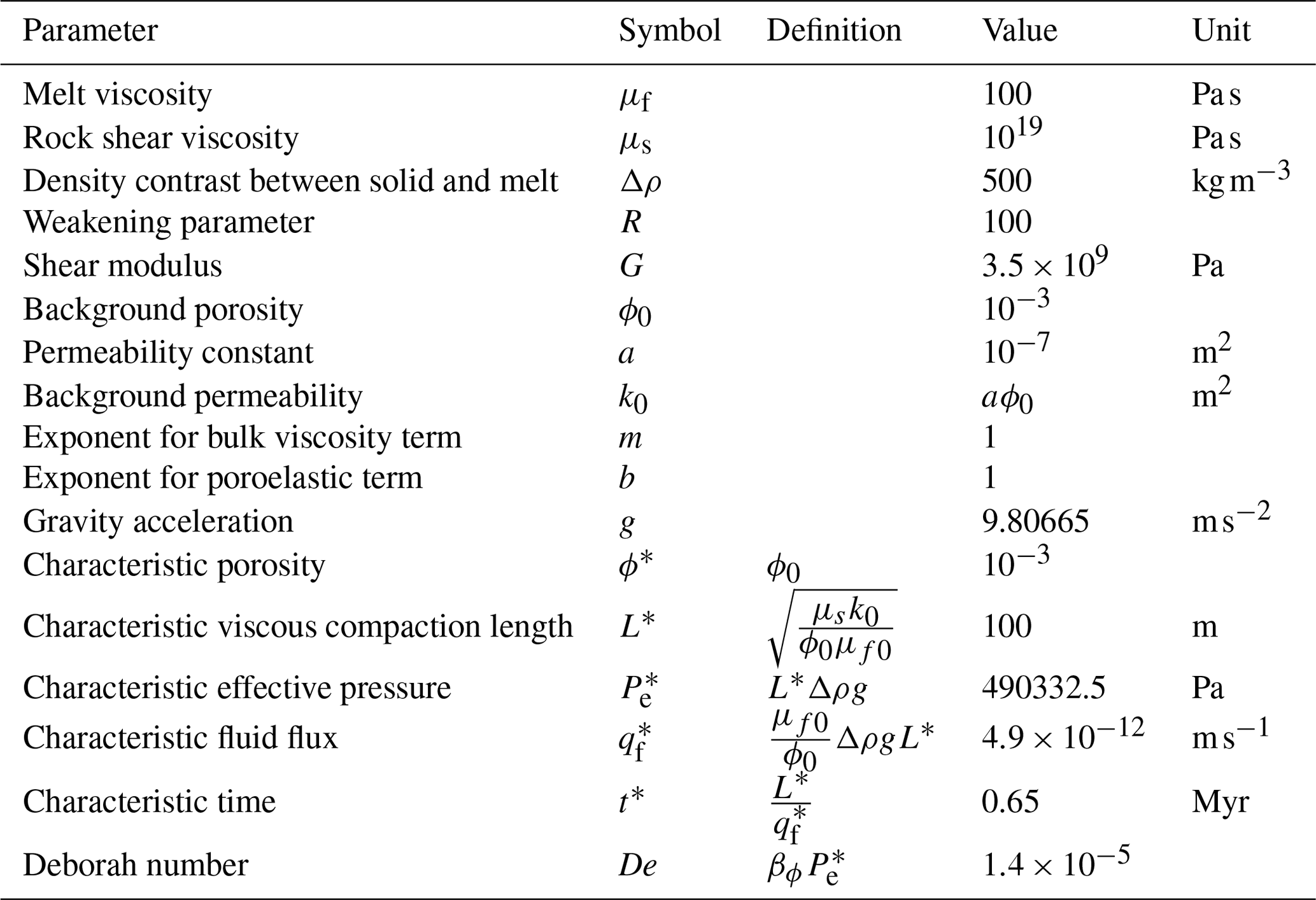
Table 3 Parameters and corresponding scaling variables used in the models. Definitions of the scaling variables are from McKenzie (1984) and Connolly and Podladchikov (1998).

5.2 Non-dimensionalisation and numerical approach

To mitigate numerical errors, a dimensionless scaling of the system is applied. The scaling variables are defined in Table 3. Using the scaling variables with Eqs. (17), (18), (20), and (21) and rearranging, we obtain the dimensionless system of equations:

$$\begin{array}{}\text{(22)}& {\displaystyle }\begin{array}{rl}{\displaystyle \frac{\partial p}{\partial t_c}}& ={\displaystyle \frac{\mathrm{1}}{{\mathit{\phi }}^b\mathit{De}}}\times \left(\mathrm{\nabla }\cdot \left[{\mathit{\phi }}^n\left(\mathrm{\nabla }p+\mathrm{1}\right)\right]\right.\\ & \left.-{\displaystyle \frac{\mathit{\phi }p}{\frac{\mathrm{1}}{R}-H\left(p\right)(\frac{\mathrm{1}}{R}-\mathrm{1})}}\right),\end{array}\text{(23)}& {\displaystyle \frac{\partial \mathit{\phi }}{\partial t_c}}=-\left[{\displaystyle \frac{\mathit{\phi }p}{\frac{\mathrm{1}}{R}-H\left(p\right)(\frac{\mathrm{1}}{R}-\mathrm{1})}}+{\mathit{\phi }}^b\mathit{De}{\displaystyle \frac{\partial p}{\partial t_c}}\right],\text{(24)}& {\displaystyle }\mathrm{\nabla }\cdot {\mathit{u}}_{\mathbf{s}}={\displaystyle \frac{\partial \mathit{\phi }}{\partial t_c}},\text{(25)}& {\displaystyle }{\mathit{u}}_{\mathbf{f}}={\mathit{\phi }}^{n-\mathrm{1}}\left(\mathrm{\nabla }p+\mathrm{1}\right)+{\mathit{u}}_{\mathbf{s}},\end{array}$$

where φ, p, t_c, u_s, and u_f are the dimensionless porosity, the dimensionless effective pressure, the dimensionless time, the dimensionless solid velocity, and the dimensionless fluid velocity, respectively. The Deborah number De is formally the ratio of the relaxation time to the observation time (Reiner, 1964), and here it characterises the ratio between viscous and elastic deformation. In the limit of small porosities, u_s can be neglected and only Eqs. (22), (23), and (25) are here solved.

Equations (22) and (23) are strongly coupled and highly stiff due to the non-linearity of the system and require an efficient numerical solver. DifferentialEquations.jl (Rackauckas and Nie, 2017), a robust ordinary differential equation (ODE) solver package, was used. This package has the advantage of simplicity, both in concept and in coding, and allows arbitrary orders of accuracy in time to be easily tested using different ODE solvers.

Equations (22) and (23) are first discretised in space using finite differences on a uniform Cartesian grid in 2D and then integrated in time using the trapezoidal rule with the second-order backward difference formula (TR-BDF2) scheme, an implicit scheme suitable for highly stiff problems (Bank et al., 1985) using DifferentialEquations.jl. It uses adaptive time-stepping and the Newton–Raphson method as a non-linear solver, using forward automatic differentiation to compute the Jacobian matrix (Revels et al., 2016). Knowing φ and p, Eq. (25) is then solved to compute u_f at each time step. The boundary conditions are periodic in all directions for all models. The system is then dimensionalised back.

5.3 Application to magmatic system

To assess the behaviour of the four advection schemes coupled with a two-phase flow system, we model the ascent of a magmatic anomaly. The spatial domain is a 2D regular grid of 450 by 900 m, and the total physical time is 1.5 Myr. The initial melt fraction distribution is defined using the following 2D Gaussian function:

$$\mathit{\varphi }={\mathit{\varphi }}_{\mathrm{0}}+{\mathit{\varphi }}_{\text{max}}\times \exp \left(-{\displaystyle \frac{(x-x_{\mathrm{0}}{)}^{\mathrm{2}}+(z-z_{\mathrm{0}}{)}^{\mathrm{2}}}{{\mathit{\sigma }}^{\mathrm{2}}}}\right),$$

with ϕ₀ the background porosity defined as 0.1 %, ϕ_max the maximum porosity defined as 5 %, and x₀ and z₀ the centre of the anomaly. The standard deviation σ of the Gaussian is 30 m. All physical parameters and corresponding scaling variables used are reported in Table 3. The evolution of porosity is shown in Fig. 8. All models were performed on a single computer with an Intel Xeon Gold 6128 processor and 128 GB of RAM using Julia version 1.10.2. All models were computed on a CPU with multithreading using 24 threads.

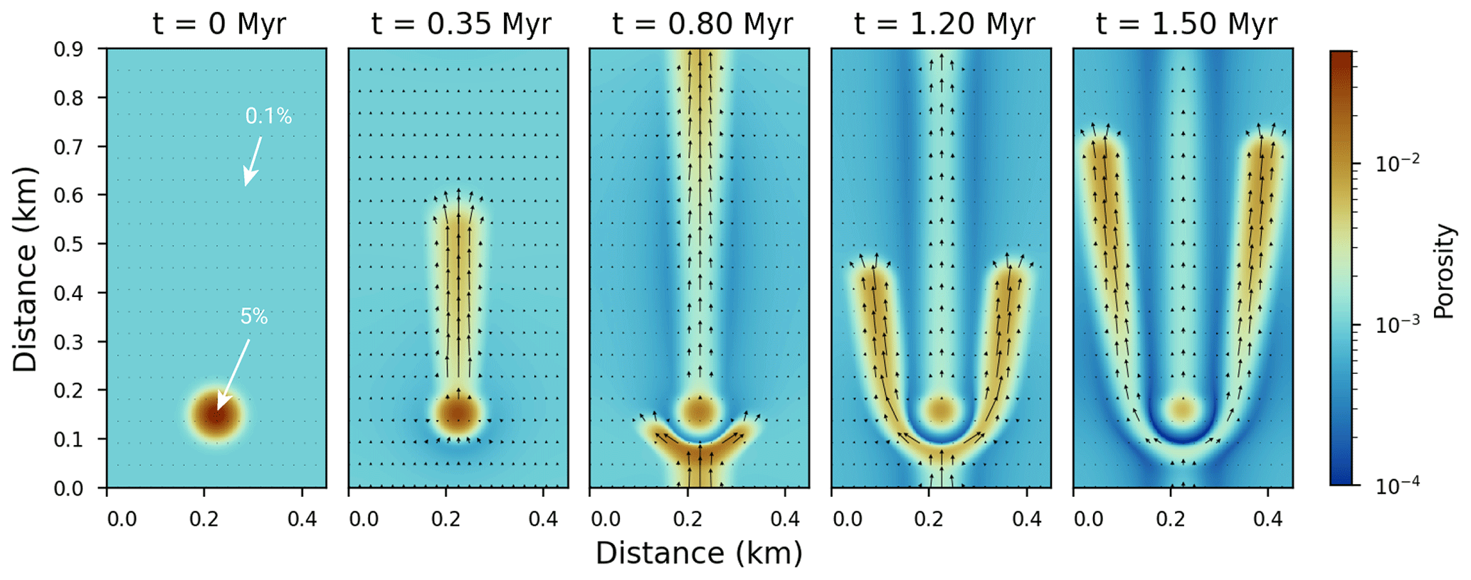
Figure 8 Reference evolution of the porosity in a 2D model from an initial Gaussian anomaly, which forms porosity waves. The superimposed vector field shows the melt velocity. Periodic boundaries are applied on all sides. The initial porosity anomaly is a Gaussian function with a maximum value of 5 %. The background porosity is 0.1 %. The spatial resolution of the grid is 300×600. The physical parameters used are listed in Table 3. The melt velocity is scaled by relative magnitude.

The melt fraction is associated with two different arbitrary chemical compositions: a basaltic composition for the background melt fraction and an andesitic composition for the anomaly, corresponding to a circle with a radius of 60 m. The aim is not to model a realistic magmatic system but to investigate how the advection schemes can numerically affect the predictions of the model. The two compositions are reported in Table 4. No feedback between the melt compositions and the physical properties of the melt was considered to prevent the advection schemes from influencing the two-phase flow. In real settings, the effect of melt composition on melt viscosity and density is not negligible for these conditions. The maximum time step allowed for the two-phase flow is constrained by the Co number associated with the melt velocity. Its maximum value allowed for the upwind and the WENO-5 schemes is 0.7, but values of 0.7 and 1.5 for the QMSL and the MIC schemes were both used to take advantage of the extended stability of these schemes. The results for the evolution of the silica content in the melt are shown in Fig. 9 for the Co number of 0.7 and for the four algorithms at a resolution of 500×1000.

Table 4 Melt compositions (in wt %) used in the models.

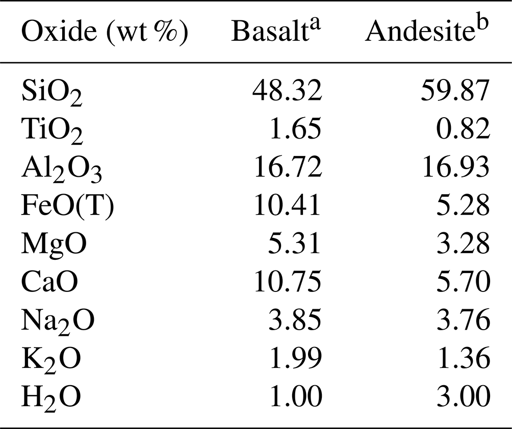
^a Recalculated from Giordano and Dingwell (2003). ^b Recalculated from Neuville et al. (1993).

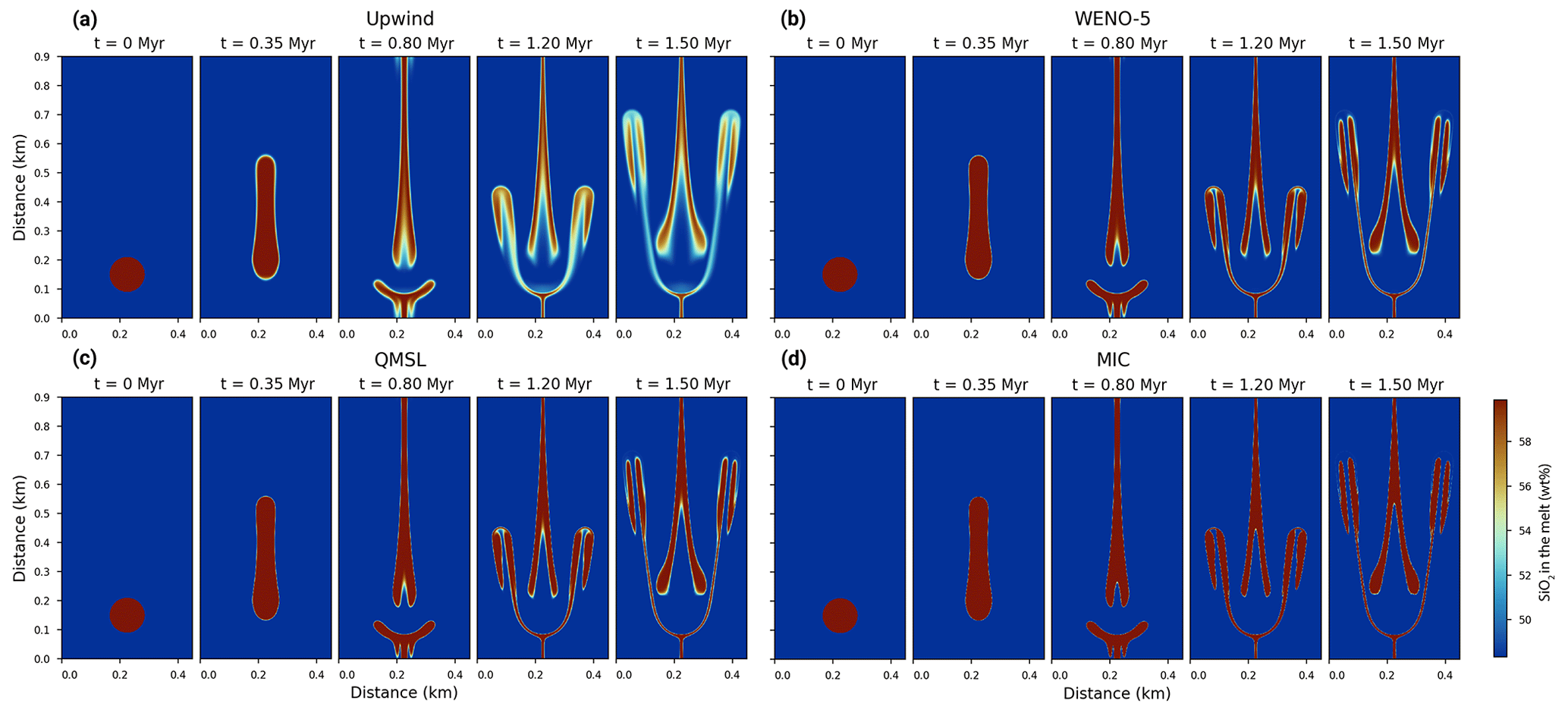
Figure 9 Evolution of the silica content in the melt for four different advection schemes: the upwind, the WENO-5, the QMSL, and the MIC (a–d) schemes. The Gaussian anomaly of porosity is associated with an andesitic composition, whereas the background porosity has a basaltic composition. The corresponding two-phase flow has an adaptive time step limited to a maximum value of a Courant number below 0.7 for all algorithms. The spatial resolution is 500×1000 nodes. The physical parameters used for the two-phase flow are reported in Table 3 and are identical for all models.

As there is no analytical solution to this particular problem, it is not possible to directly calculate the numerical error in the different advection schemes. Nevertheless, we can compute the mass conservation of the advected quantities. The total mass of the melt composition is conserved, as it is re-normalised to 100 % at each time step. This is a constant-sum constraint and is characteristic of compositional data (Aitchison, 1982). However, it is not necessarily the case for each individual oxide. In that light, similar to Eq. (14), we monitor the mass conservation of each individual oxide M_ox in the melt at each time step:

$$M_{\text{ox}}={\displaystyle \frac{\sum _{k=\mathrm{1}}^K\left({\mathit{\varphi }}^k{C}_{\text{ox}}^k\right)}{\sum _{k=\mathrm{1}}^K\left({\mathit{\varphi }}_{\mathrm{0}}^k{C}_{{\text{ox}}_{\mathrm{0}}}^k\right)}},$$

where ϕ^k and ${\mathit{\varphi }}_{\mathrm{0}}^k$ are the current and initial porosity at index k, and $C_{\text{ox}}^k$ and $C_{{\text{ox}}_{\mathrm{0}}}^k$ are the current and initial composition of the oxide of interest in the melt at index k.

The melt fraction ϕ is conserved through the models, as Eqs. (22) and (23) are solved using a conservative discretisation. Therefore, M_ox only monitors the effects of the advection schemes for the oxide of interest. To quantify how the mass conservation evolves for each individual oxide and for each advection algorithm, the same model was performed at five different resolutions: 100×200, 200×400, 300×600, 400×800, and 500×1000. The values of the mass conservation of silica content $M_{{\text{SiO}}_{\text{2}}}$ for each resolution are shown in Fig. 10 for all the models. The values of the mass conservation of each oxide for all the algorithms are shown in Fig. 11. The total running time of each model is reported in Fig. 12.

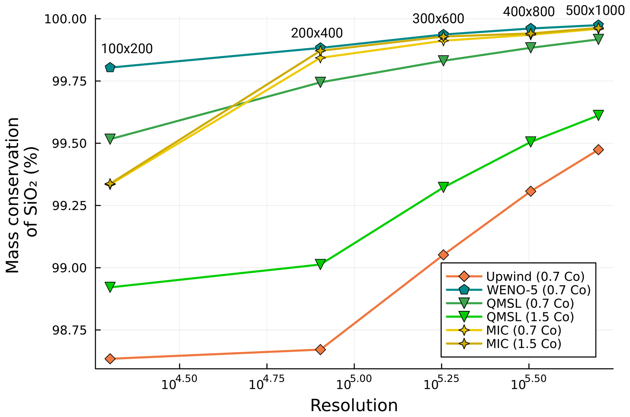
Figure 10 Mass conservation of silica content in the melt fraction for four different advection schemes and five different spatial resolutions at the end of each simulation. The Courant number used is 0.7 for the WENO-5 and the upwind schemes and 0.7 or 1.5 for the QMSL and the MIC schemes. The resolutions are 100×200, 200×400, 300×600, 400×800, and 500×1000. The physical parameters used are reported in Table 3.

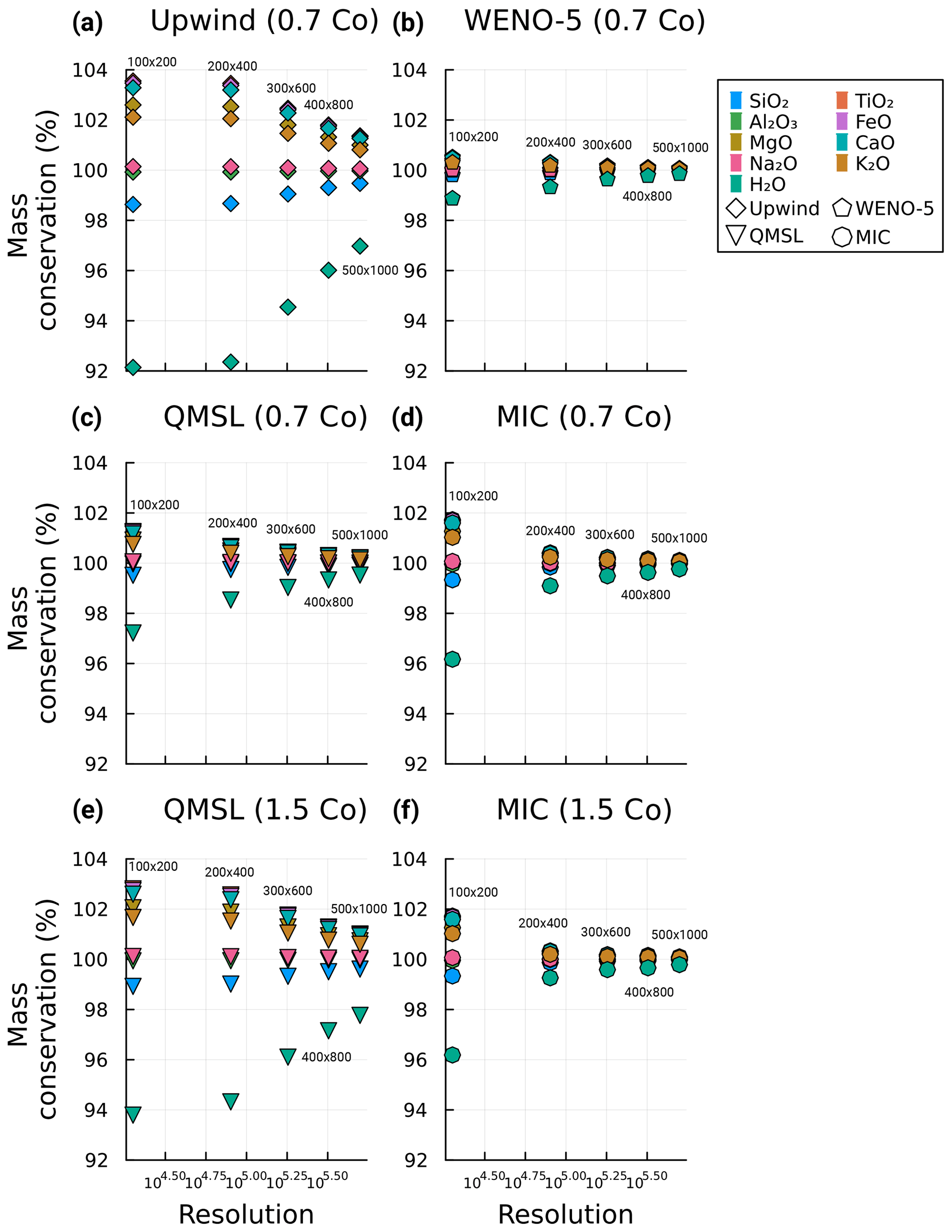
Figure 11 Mass conservation of each oxide in the melt fraction for four different advection schemes and five different spatial resolutions at the end of each simulation. The Courant number used is 0.7 for the WENO-5 and the upwind (a, b) schemes and 0.7 or 1.5 for the QMSL and the MIC (c–f) schemes. The resolutions are 100×200, 200×400, 300×600, 400×800, and 500×1000. The physical parameters used are reported in Table 3.

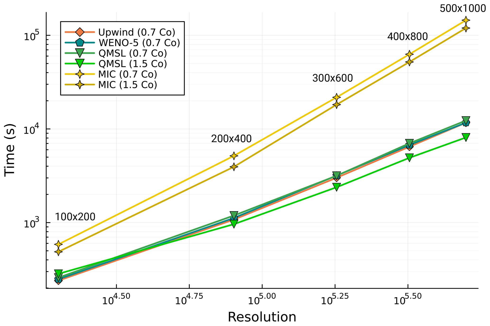
Figure 12 Total running time of the two-phase flow system coupled with four different advection schemes and five different resolutions. The Courant number used is 0.7 for the WENO-5 and the upwind schemes and both 0.7 and 1.5 for the QMSL and the MIC schemes. The resolutions are 100×200, 200×400, 300×600, 400×800, and 500×1000. The physical parameters used are reported in Table 3. All models were performed using a single computer with an Intel Xeon Gold 6128 processor and 128 GB of RAM using Julia version 1.10.2. All advection algorithms were computed on a CPU with multithreading using 24 threads.

6 Results and discussion

The numerical models produced allow a better understanding of the process of passive chemical transport in magma within porosity waves and the impact of each advection scheme on the magma composition over time. All models confirm two distinct composition domains at the top of the porosity waves at the end of the simulations (Fig. 9). It is effectively a mixing of the compositions from the initial background porosity and from the anomaly. This is because melt is incorporated by the waves as they rise. This is attributed to the fact that the velocity of the porosity waves is higher than the melt velocity and has also been reported in previous studies (e.g. Jordan et al., 2018).

Comparing the results of the four algorithms, it is clear that the upwind scheme has the highest amount of numerical diffusion, which increases chemical mixing for non-physical reasons. The WENO-5 and QMSL exhibit similar results in terms of numerical diffusion, while the MIC shows the lowest amount with almost purely advective behaviour (Fig. 9). This is consistent with the numerical tests (Figs. 6 and 7). In terms of mass conservation, the oxide content is not conserved in all four schemes (Figs. 10 and 11). The WENO-5 gives the best results, with a mass conservation ranging from 98.87 % to 100.51 % for the lowest resolution to 99.85 % to 100.06 % at the highest resolution for all the oxides. The MIC performs similarly at high resolution, ranging from 99.77 % to 100.11 % for all the oxides at the highest resolution and with a significant increase in mass conservation from the 200×400 resolution. An improvement in the mass conservation for a Co number of 1.5 compared to the value of 0.7 is also noticeable. The QMSL shows slightly lower mass conservation for a Co of 0.7, ranging from 99.52 % to 100.22 % at the highest resolution and 97.22 % to 101.26 % at the lowest. In contrast to the MIC, there is a significant decrease for the mass conservation for a Co number of 1.5, ranging from 97.22 % to 102.81 % at low resolution to up to 97.77 % to 101.01 % at high resolution. The upwind scheme shows the worst values for mass conservation, ranging from 92.14 % to 103.55 % at low resolution to values of 96.97 % to 101.37 % at the highest resolution (Figs. 10 and 11). The better mass conservation of the MIC for a higher Co number can be explained by less reseeding and removal of markers, as the approach used is not mass conservative. On the other hand, the poorer performance concerning the QMSL at higher Co number can be interpreted as showing the decrease in accuracy of the trajectory tracing with increasing time step. The differences in mass conservation observed in the different oxides through all the models show that the initial conditions play a role and that higher values in the anomaly at the beginning of the model leads to a loss of mass (e.g. SiO₂ or Al₂O₃), whereas the opposite leads to an excess of mass (e.g. CaO or K₂O). Also, the greater the relative difference between the composition of the oxide from the anomaly and the background melt fraction, the greater the mass conservation loss or gain (e.g. H₂O or FeO). However, it is observed that the mass conservation of all the oxides appears to converge towards 1 with increasing resolution for all methods.

In terms of performance, all schemes, except the MIC, show a run time of the same order of magnitude for a Co number of 0.7 at all resolutions. This is explained by the multithreading approach, which allows high performance, even for more computationally expensive algorithms due to parallelism. The high computational cost of the MIC is mainly attributed to the reseeding and removal of the markers due to the highly divergent velocity field. This part was not fully parallelised due to race conditions caused by the removal and addition of memory at run time. Also, the MIC and QMSL perform better for a Co number of 1.5 compared to 0.7 (Fig. 12). This is explained by a larger adaptive time step used by the two-phase flow solver due to the extended stability domain, which means that fewer time steps are required to solve the system. All the calculations were performed on a single CPU, and the code could be further optimised, especially for the MIC. However, this result provides an idea of the cost of each method when parallelised and highlights the complexity of fully parallelising a MIC algorithm while dealing with a significant amount of reseeding and marker removal.

The upwind scheme is considered inadequate for this problem due to its high numerical diffusion, and its lack of mass conservation for highly divergent velocity fields. The MIC scheme shows very good results in terms of accuracy with the least amount of numerical diffusion and has no stability condition. It also demonstrates better mass conservation with a higher time step. However, it is expensive in terms of computation and memory, as it needs to keep track of the markers. As the velocity field v_f is strongly divergent, it requires frequently regenerating and deleting markers, which adds complexity to the implementation and additional numerical cost. As a result, we consider this scheme to be too costly for this particular problem but recognise its robust qualities for other geodynamic problems where diffusion is not acceptable, such as thermomechanical deformation or mantle convection (e.g. Duretz et al., 2011; Ueda et al., 2015; Trim et al., 2020). On the other hand, the QMSL scheme shows very good performance with its extended stability field and good accuracy but has very poor mass conservation for a high Co, which contradicts the purpose of this scheme. A potential approach to improve the mass conservation would be to improve the trajectory tracing step, either by using higher-order multistep methods (e.g. Filbet and Prouveur, 2016) or by using Runge–Kutta schemes, similar to the one used for the MIC. On the basis of these results, the WENO-5 advection scheme appears to be the most appropriate for this problem. Mass conservation is a critical property for studying mass balance and mass transport problems associated with magma transport at different scales on Earth, and this algorithm obtains the best results. It also has good accuracy and reasonable performance and is easy to extend to higher dimensions and to parallelise.

7 Conclusions

In this study, a series of tests were carried out to determine which advection scheme is the most suitable for modelling the chemical transport of magma. Four of the most commonly used algorithms in the literature were compared: the upwind, WENO-5, MIC, and QMSL schemes. To test them, we combined a 2D two-phase flow model, which describes the evolution of the melt fraction of magma over time, with the chemical advection of its composition.

All algorithms, with the exception of the upwind scheme, are able to predict the melt composition with reasonable accuracy. However, mass conservation of each individual oxide in the melt is not fully achieved for any of the schemes. The MIC, while showing the least amount of numerical diffusion, requires a very large amount of reseeding and removal of markers due to the strongly divergent melt velocity field. This procedure is costly and requires reallocating memory at run time, complicating the implementation. The QMSL scheme has the worst mass conservation of the three algorithms, especially at high Co. This could potentially be improved by refining the trajectory tracing step to make it a more valuable alternative. The WENO-5 scheme shows the best results in mass conservation, even at low resolutions, is explicit, is easy to implement, and extends in 3D, although it is constrained by the CFL condition. On the basis of these results, the WENO-5 scheme is the most suitable to use for transporting magma composition during magma ascent. This is also applicable to problems using similar formulations, such as chemical advection in aqueous fluids, and makes WENO-5 a suitable scheme for modelling reactive transport under crustal or mantle conditions.