the Creative Commons Attribution 4.0 License.
the Creative Commons Attribution 4.0 License.
 | 15 Aug 2024
Implementation of a brittle sea ice rheology in an Eulerian, finite-difference, C-grid modeling framework: impact on the simulated deformation of sea ice in the Arctic
Laurent Brodeau
Pierre Rampal
Einar Ólason
Véronique Dansereau
We have implemented the brittle Bingham–Maxwell sea ice rheology (BBM) into SI3, the sea ice component of NEMO. After discussing the numerical aspects and requirements that are specific to the implementation of a brittle rheology in the Eulerian, finite-difference, Arakawa C-grid framework, we detail the approach we have used. This approach relies on the introduction of an additional set of prognostic stress tensor components, sea ice damage, and sea ice velocity vector, following a grid point arrangement that expands the C-grid into the Arakawa E-grid. The newly implemented BBM rheology is first assessed by means of a set of idealized SI3 simulations at different spatial resolutions. Then, sea ice deformation rates obtained from simulations of the Arctic at a ° spatial resolution, performed with the coupled ocean–sea ice setup of NEMO, are assessed against satellite observations. For all these simulations, results obtained with the default current workhorse setup of SI3 are provided to serve as a reference. Our results show that using a brittle type of rheology, such as BBM, allows SI3 to simulate the highly localized deformation pattern of sea ice, as well as its scaling properties, from the scale of the model's computational grid up to the basin scale.
- Article
(9491 KB) - Full-text XML
- BibTeX
- EndNote


Sea ice impacts the ocean and the atmosphere at both the local and the regional scale (Vihma, 2014; IPCC, 2022). In polar regions, the sea ice cover modulates the radiative and turbulent exchanges of heat, fresh water, gas, and momentum between the ocean and the atmosphere (e.g., Taylor et al., 2018, for a review). At the local scale, these fluxes are predominately controlled by the heterogeneity of the sea ice thickness, which itself is governed by the sea ice dynamics and the associated formation of leads and ridges. This stresses the relevance of accurately representing sea ice dynamics in simulations of the coupled multi-component Earth system, such as regional and global climate simulations, and even for short-term sea ice predictions.
The dynamical behavior of sea ice is controlled by processes that interact and evolve over a wide range of spatial and temporal scales. This multiscale nature of sea ice physics is fascinating and has triggered the curiosity of geophysicists since the early 1970s (Coon et al., 1974). More recently, scientific interest in sea ice dynamics has grown significantly due to the dramatic retreat and thinning of the Arctic sea ice cover. In addition, the abundance of new observations of sea ice kinematics, recorded by both in situ instruments (e.g., the buoy trajectories of the International Arctic Buoy Program, https://iabp.apl.uw.edu/data.html, last access: 30 July 2024) and satellites (e.g., the ice trajectories from the RADARSAT Geophysical Processor System; Kwok et al., 1998), has the potential to foster additional advancements in sea ice modeling.
The dynamics of sea ice is complex. For instance, Rampal et al. (2008) and Weiss et al. (2009) showed that the statistical properties of sea ice deformation are characterized by a coupled space–time multi-fractal scaling invariance, similar to what is observed for the deformation of the Earth's crust (Kagan and Jackson, 1991; Marsan and Weiss, 2010). The spatial and temporal scaling properties of sea ice deformation and their coupling provide evidence for the strong heterogeneity and intermittency that characterizes sea ice dynamics (Rampal et al., 2008).
Reproducing the discontinuous nature of sea ice – related to the presence of fractures and leads – in continuous sea ice models, as well as the complexity of the spatial patterns and temporal evolution of these features, poses a fundamental and major challenge (e.g., Bouchat et al., 2022; Hutter et al., 2022). As an effort to tackle this challenge, Dansereau et al. (2016) introduced the Maxwell elasto-brittle rheology (MEB). MEB was implemented into neXtSIM, a large-scale dynamical–thermodynamical Lagrangian finite-element sea ice model (Rampal et al., 2016), and used to evaluate the performance of this new rheology in a realistic pan-Arctic simulation. Wintertime sea ice deformations simulated by MEB in neXtSIM were first evaluated statistically against satellite observations, in terms of probability density functions (PDFs) and scaling invariance properties, in Rampal et al. (2016, 2019) and later in the two companion papers of Bouchat et al. (2022) and Hutter et al. (2022), showing satisfying results.
Recently, Ólason et al. (2022) introduced the brittle Bingham–Maxwell rheology (BBM) as an effort to address the incomplete treatment of the convergence of highly damaged sea ice in MEB. This deficiency of MEB results in the unrealistic representation of the ice thickness after a couple of years of model integration. Indeed, recent realistic BBM-driven multidecadal simulations performed with neXtSIM have been shown to reproduce (i) the scaling properties of sea ice deformation from the model grid cell up to the scale of the Arctic basin and (ii) the thickness pattern of the sea ice cover well when compared to observations (Ólason et al., 2022; Boutin et al., 2023).
Yet, performing coupled ocean–sea ice or Earth system CMIP-like simulations with neXtSIM in a numerically efficient manner remains challenging because the numerical coupling of neXtSIM to a third-party – generally Eulerian – GCM component requires the implementation of a relatively inefficient Lagrangian–Eulerian coupling strategy. Furthermore, the weak scalability capabilities of neXtSIM when run in parallel on more than a few tenths of processors and/or at spatial resolutions typically below 10 km have been shown to substantially hinder the scalability of coupled setups (Samaké et al., 2017). Thus, the implementation of BBM into an Eulerian CMIP-class sea ice model, such as SI3 of NEMO, has the potential to significantly benefit the sea ice, ocean, and climate modeling communities. First, it will facilitate the assessment of the sensitivity of the simulated sea ice dynamics to the type of rheology used in a modeling framework that these communities are familiar with. And second, the good scalability capabilities of NEMO (Tintó Prims et al., 2019) will allow performing realistic kilometer-scale simulations that use a brittle rheology.
As of today, a few efforts have been made to implement MEB in sea ice models comparable to SI3 in terms of discretization method and grid, such as the MIT general circulation model (Losch et al., 2010), or LIM, the former sea ice component of the NEMO modeling system (Rousset et al., 2015). And more recently, Plante et al. (2020) have successfully implemented MEB in the McGill sea ice model (Tremblay and Mysak, 1997; Lemieux et al., 2008, 2014). Overall, the work of these modeling groups has highlighted some challenging aspects that are specific to the implementation of a brittle rheology in a realistic Eulerian model that uses the finite-difference method on a staggered grid. As suggested by the work of Plante et al. (2020), when discretized on the Arakawa C-grid (Arakawa and Lamb, 1977), the same grid as used by SI3 (Vancoppenolle et al., 2023), brittle rheologies seem to be more prone to numerical instabilities than their viscous–plastic counterparts. In particular, they report that the stability of their MEB implementation is sensitive to the resort to spatial averaging, an interpolation technique that is traditionally used to relocate certain fields between the staggered points of the grid. Moreover, the need to advect the stress tensor, specific to brittle rheologies, poses another challenge when using the C-grid because it demands the advection of a scalar field, namely the shear element of the stress tensor, that is defined at the corner points of the grid cell.
In this paper, we propose a new discretization approach adapted to the numerical implementation of a brittle rheology in an Eulerian finite-difference, C-grid-based sea ice model. We describe how we have implemented this new approach into SI3 based on the expansion of the C-grid into an Arakawa E-grid.
As a first validation step of our BBM implementation, we discuss SI3 results obtained using the idealized test case setup of Mehlmann et al. (2021) at different horizontal resolutions. Then, as the second step, we compare the sea ice deformations obtained from realistic coupled ocean–sea ice simulations of the pan-Arctic against those constructed from satellite observations. To serve as a reference, the results of simulations run using the default workhorse setup of SI3 (based on the aEVP rheology of Kimmritz et al., 2016) are also included in both validation steps.
This paper is organized as follows. In Sect. 2, we summarize the equations of the sea ice dynamics model, discuss the aspects in which the numerical implementation of a brittle rheology may differ from that of a non-brittle viscous–plastic one, and detail the numerical aspects specific to our implementation of BBM into SI3. In Sect. 3, we describe the technical aspects of our SI3 simulations and discuss the results obtained with both the idealized and pan-Arctic configurations. In Sect. 4, we discuss some numerical aspects of our implementation and some limitations of the BBM rheology. Our conclusions are summarized in Sect. 5. Detailed nomenclature relating the acronyms and symbols used throughout the paper is outlined in Appendix A.
2.1 Governing equations and constitutive law
The two-dimensional, vertically integrated, momentum equation for sea ice reads
where m is the mass of ice and snow per unit area, u is the ice velocity vector, h is the ice thickness, σ is the internal stress tensor, A is the sea ice fraction, τa is the wind stress vector, τ is the ocean current stress, f is the Coriolis frequency, k is the vertical unit vector, g is the acceleration of gravity, and H is the sea surface height. In the two-dimensional (plane stresses) case, the stress tensor is written as
In general, a constitutive law relates σ to the strain rate tensor , defined as follows:
As derived by Ólason et al. (2022) (their Eq. 20), the BBM constitutive model yields
where E and λ are the elastic modulus and apparent viscous relaxation time of the ice, K is the elastic stiffness tensor, is a term introduced to prevent excessive ridging (see below), and d is the damage scalar: a variable that represents the density of fractures in the ice at the subgrid scale. The underbar notation indicates that the tensors are expressed in their Voigt form. E and λ are modulated by the sea ice concentration and damage as
where C is the compaction parameter constant and α is a constant exponent greater than 1. α fulfills the physical constraint that the relaxation time for the stress also decreases as damage increases and re-increases as the ice heals (i.e., damage decreases) because the material respectively loses and recovers the memory of reversible deformations (Dansereau et al., 2016).
The BBM constitutive model in Eq. (4) only differs from that of MEB through the inclusion of the term : a threshold between reversible and permanent deformation regimes. As noted by Ólason et al. (2022), the inclusion of this term prevents the excessive convergence that is occurring in MEB simulations lasting longer than a season. For convergent stresses in the range , the deformation is elastic; otherwise, it is visco-elastic. Ólason et al. (2022) interpret this threshold as the maximum pressure the ice can withstand before ridging. They consequently choose to let the ridging threshold, Pmax, be proportional to the ice thickness to the power (Hopkins, 1998) and depend exponentially on the concentration (Hibler, 1979), i.e.,
where σI is the (isotropic) normal stress and Pmax is the ridging threshold defined as
We follow Dansereau et al. (2016) and Ólason et al. (2022) in using a two-step approach to solve Eq. (4). As the first step, an initial estimate of , denoted as , is calculated assuming no change in damage:
Then, as the second step, the following test and adjustment are performed on the state of stress: if is locally over-critical, i.e., located outside of the Mohr–Coulomb damage criterion (Fig. 1), an increment in ice damage, dcrit, is applied such that
where is the local value of the over-critical stress, and is the corresponding post-failure (i.e., post-damage) stress. As discussed in Dansereau et al. (2016) and Plante and Tremblay (2021), dcrit is used to scale over-critical stresses back towards the Mohr–Coulomb damage criterion, assuming viscous relaxation to be negligible during the (comparatively very fast) damage process. The associated temporal evolution of the damage and adjustment of the stress state is given by
where td is a characteristic timescale for damage propagation. In the BBM framework, dcrit is expressed as follows:
where c is the cohesion, and μ is the friction coefficient. The threshold N is used to prevent any numerical instability at very high normal stresses and is set large enough not to impact the solution noticeably. As suggested by Rampal et al. (2016), a slow restoring process is applied to the damage to account for the healing of ice under refreezing conditions. The rate of decrease of the damage associated with this refreezing is taken to be proportional to ΔTh, the temperature difference between basal and surface ice:
where kth is the healing constant. This process can be decoupled from Eq. (11) due to the large separation of timescales between the healing and damaging processes.
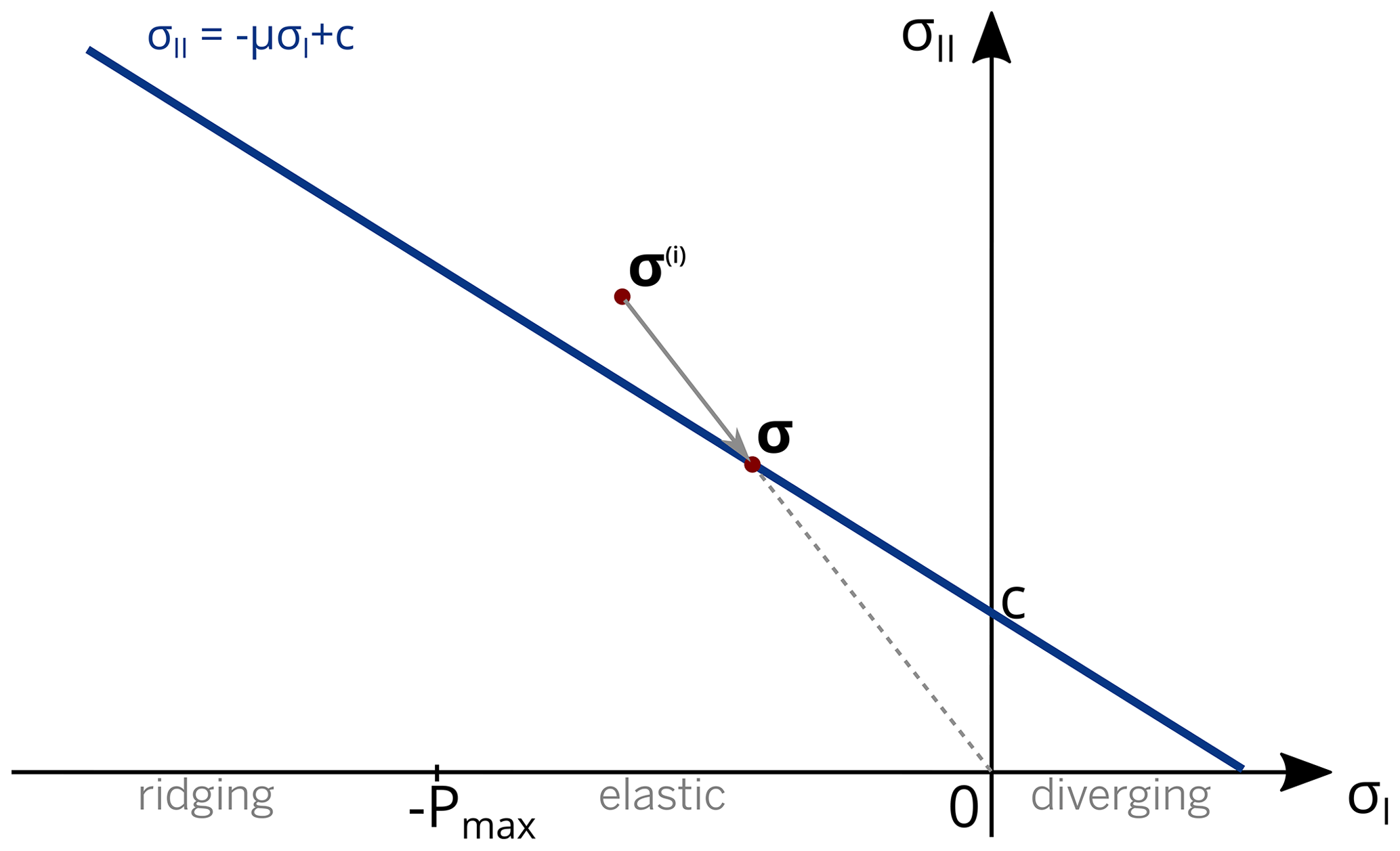
Figure 1Mohr–Coulomb yield envelope in the internal stress invariant coordinates (blue line). Illustration of how an over-critical stress state σ(i) (initial estimate) is evolving (gray arrow) towards the corrected state σ when using the BBM rheology.
2.2 Numerical implementation: brittle versus viscous–plastic rheologies
To understand the extent to which the numerical implementation of a brittle rheology differs from that of a viscous–plastic one, let us first review the main differences between these rheologies and their respective classical numerical implementation.
First, the elasto-visco-brittle family of rheologies (MEB, BBM; Dansereau et al., 2016; Ólason et al., 2022) considers unfragmented sea ice to be an elastic and damageable solid. Fragmented sea ice is a visco-elastic material in which irreversible deformations dissipate the stresses. As opposed to viscous–plastic frameworks, elasticity is therefore a physical and non-negligible component of the model. It is modulated by the level of damage, d, which keeps the memory of the state of fragmentation of the sea ice cover. The combination of elasticity and damage, even if treated in an isotropic manner, naturally simulates a strong anisotropy and localization of the deformation, down to the nominal spatial and temporal scale (i.e., the grid resolution and time step of the model, respectively; Dansereau et al., 2016; Weiss and Dansereau, 2017; Rampal et al., 2019; Ólason et al., 2022). Therefore, all the mechanically related fields, such as damage, concentration, thickness, and velocity, tend to exhibit very sharp gradients. Second, in the BBM (as in the MEB) framework, a twofold approach is used to linearize the system of equations and solve the coupled constitutive and damage evolution equations: (i) an initial estimate, in which stress components are updated based on the constitutive law (Eq. 9), and (ii) a damage step in which the Mohr–Coulomb test is performed, resulting in a potential adjustment of local over-critical stresses and the associated increase in damage (Fig. 1, Eqs. 11 and 12). In viscous–plastic rheologies, which do not incorporate damage, no such twofold approach is necessary to solve the system of dynamical equations.
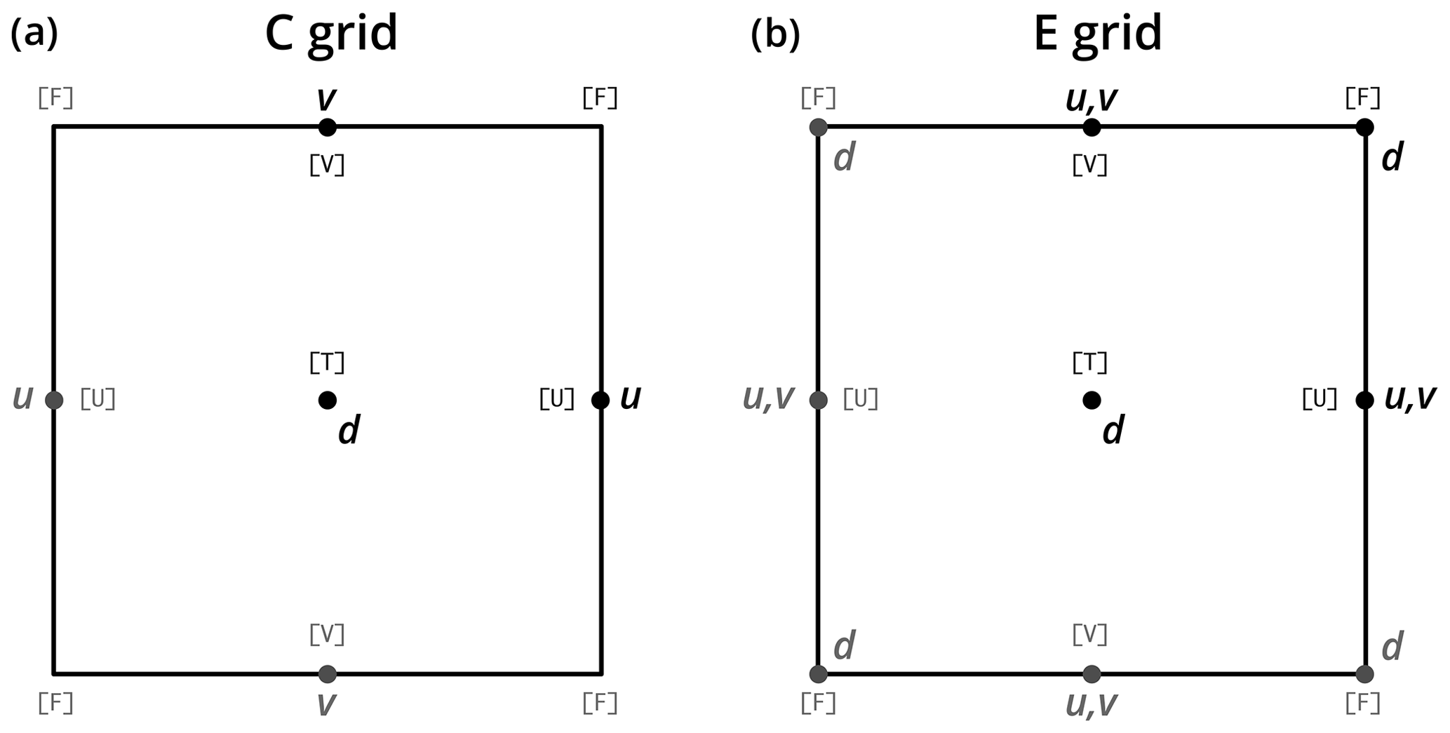
Figure 2Point arrangement and staggering in a grid cell: (a) the C-grid as used in NEMO and (b) the E-grid. The letter d indicates the location of tracers, while the letters u and v indicate that of the i- and j-wise components of the velocity vector. Letters in brackets indicate the name of the grid points as referred to throughout the paper.
A third and major difference between the two types of model is that in brittle models, the stress tensor σ is a prognostic variable, while it is a diagnostic variable in viscous–plastic models. This implies that the implementation of a brittle rheology in an Eulerian framework, as opposed to that of a viscous–plastic rheology, should, in practice, consider the advection of σ, along with other – typically scalar – tracers (see Sect. 2.4). One could argue that, based on a scale analysis, the advection terms of the stress tensor components are somewhat negligible and that it is therefore acceptable to simply omit these terms (similarly to what is done for the ice velocity in the momentum equations). While these terms are indeed very small, we think that it is important to include them in the Eulerian implementation of a brittle model because of the strong interdependence that bounds the damage tracer and the stress tensor. This interdependence is the consequence of E and λ being a function of d (Eqs. 5 and 6) in the estimate of σ(i) (Eq. 9). The damage, as a tracer that can live on for days, if not weeks, depending on the temperature conditions, has to be advected with the ice velocity, like any other tracer. As such, we think that the advection of the stress tensor is necessary to preserve the full spatial consistency between the damage tracer and the internal stress state, in particular in the case of simulations longer than a few days that involve significant sea ice displacements.
Finally, note that in their numerical implementation of BBM, Ólason et al. (2022) chose to solve the dynamics explicitly using a time step sufficiently small to account for the propagation of damage in the ice in a physically realistic manner. We follow the same approach in our implementation of BBM into SI3. Typically, this implies using a time step a few hundred times smaller (hereafter referred to as the dynamical time step, Δt) than that used for the thermodynamics and the advection (hereafter referred to as the advective time step, ΔT). This is implemented by means of a time-splitting approach. Ns, the number of (Δt-long) integrations to perform during one advective time step (ΔT), is imposed by ΔT and Δx, the horizontal resolution of the grid:
where CE is the propagation speed of an elastic shear wave and ρi is the density of ice. Note that if ΔT is already constrained by Δx, as in NEMO, the choice of Ns becomes somewhat independent of the spatial resolution at which the model is run.
2.3 Numerical implementation of the BBM rheology
SI3 uses curvilinear coordinates on a fixed Eulerian mesh, and the spatial discretization is achieved by means of the finite-difference method (FD) on the Arakawa C-grid (Arakawa and Lamb, 1977). The use of the C-grid is justified based on numerical and practical grounds, as it ensures the exact collocation of ocean and sea ice horizontal velocity components, which simplifies the coupling with the ocean component of NEMO and prevents interpolation-related errors as well as extra computational load.
As shown in Fig. 2a, on the C-grid, tracers are defined at the cell centers, hereafter referred to as the T-point, while the x and y components of vectors are defined at the center of the right-hand and upper edges of each cell, respectively (hereafter U-point and V-point). The point located at the upper-right corner of each cell, known as the vorticity point, is referred to as the F-point. In the literature, this vorticity point is sometimes located at the bottom-left corner of the cell, with the U- and V-points possibly located at the left-hand and lower edges of the cell, and is sometimes referred to as the Z-point (Losch et al., 2010; Plante et al., 2020).
Regardless of the type of rheology considered, the main challenge posed by the C-grid is a consequence of the discretized FD expressions of the elements of the strain rate tensor being staggered in space, with the trace elements and defined at the T-point and the shear rate defined at the F-point. Based on the constitutive law (Eq. 4), the same applies to the stress tensor σ. This staggering between the diagonal and off-diagonal elements of σ is appropriate when considering the discretization of the momentum equation (Eq. 1) because the discretized elements of the vector divergence of σ are then defined where they are needed: namely, at U- and V-points. However, this staggering becomes an issue whenever the parameterization of the constitutive law requires or σ12 to be known at a T-point. This is the case, for instance, for the expression of the Δ parameter in elastic–viscous–plastic (EVP) models or that of the second stress invariant σII in MEB and BBM (i.e., Eq.13), as they require and σ12, respectively, to be known at T-points. Moreover, in brittle rheologies, a value of d is required not only at the T-point, but also at the F-point to estimate E and λ (Eqs. 5 and 6) needed to update (Eq. 9). On the C-grid, a common way to interpolate a scalar defined at F-points onto T-points is to simply use the average of this scalar on the four surrounding F- points and conversely to interpolate from T- to F-points. In the aEVP implementation of SI3 (Kimmritz et al., 2016), the problem posed by the staggering of tensor elements is overcome by using this averaging approach to interpolate the square of the shear rate from F- to T-points. Later on, the term is also interpolated from T- to F-points in order to estimate σ12. In their implementation of MEB, Plante et al. (2020) also use this approach to interpolate the damage tracer at F-points. However, they report that using the same approach to estimate σ12, and hence σII, at T-points when performing the Mohr–Coulomb test (Eq. 13) results in checkerboard instabilities. The solution they propose to prevent the occurrence of these instabilities is to introduce an additional σ12 that is defined at T-points. This additional σ12 is updated at each time step using – as an increment – the average of the four σ12 increments computed at the surrounding F-points.
Note that based on the strong interdependence between the internal stress and the damage in brittle rheologies (Sect. 2.2), as well as the highly localized nature of the damage, we think that the use of the averaging technique to estimate d at the corner points of the C-grid cells should be avoided if possible. Indeed, by using such a technique, , as opposed to and , is updated using values of E and λ that have been calculated using a poorer estimate of d at the F-point than what the rheology, together with Mohr–Coulomb test, would have produced at this location if explicitly solved on the F-point. This is because the four-point average of a variable such as the damage that is highly heterogeneous in space, even at the grid point scale, cannot provide a very accurate and reliable estimate of the local value.
Finally, with the C-grid, the implementation of the advection of σ12 (F-point) in a way consistent (in terms of the advection scheme used) with that used for σ11 and σ22 (T-point) is somewhat challenging. That is because the advection of a scalar defined at the F-point, using the same scheme as that used for the advection of scalars at T-points, requires the existence of a u and a v at V- and U-points, respectively. These later considerations have prompted us to consider the use of a new spatial discretization approach for the implementation of BBM on the C-grid.
2.3.1 The E-grid approach
To avoid the interpolation of the damage and the stress components between the center and the corner points of the grid cell and allow the consistent advection of all the components of the stress tensor, an additional sea ice velocity vector, denoted as , is introduced. As shown in Fig. 3b, the x component of this additional velocity, , is defined at V-points, while its y component, , is defined at U-points. Similarly, the damage tracer is also duplicated, with an additional occurrence at the upper-right corners of the grid cell, i.e., at F-points. This grid staggering arrangement corresponds to that of the Arakawa E-grid (Arakawa and Lamb, 1977; Janjić, 1984; Maier-Reimer et al., 1993).
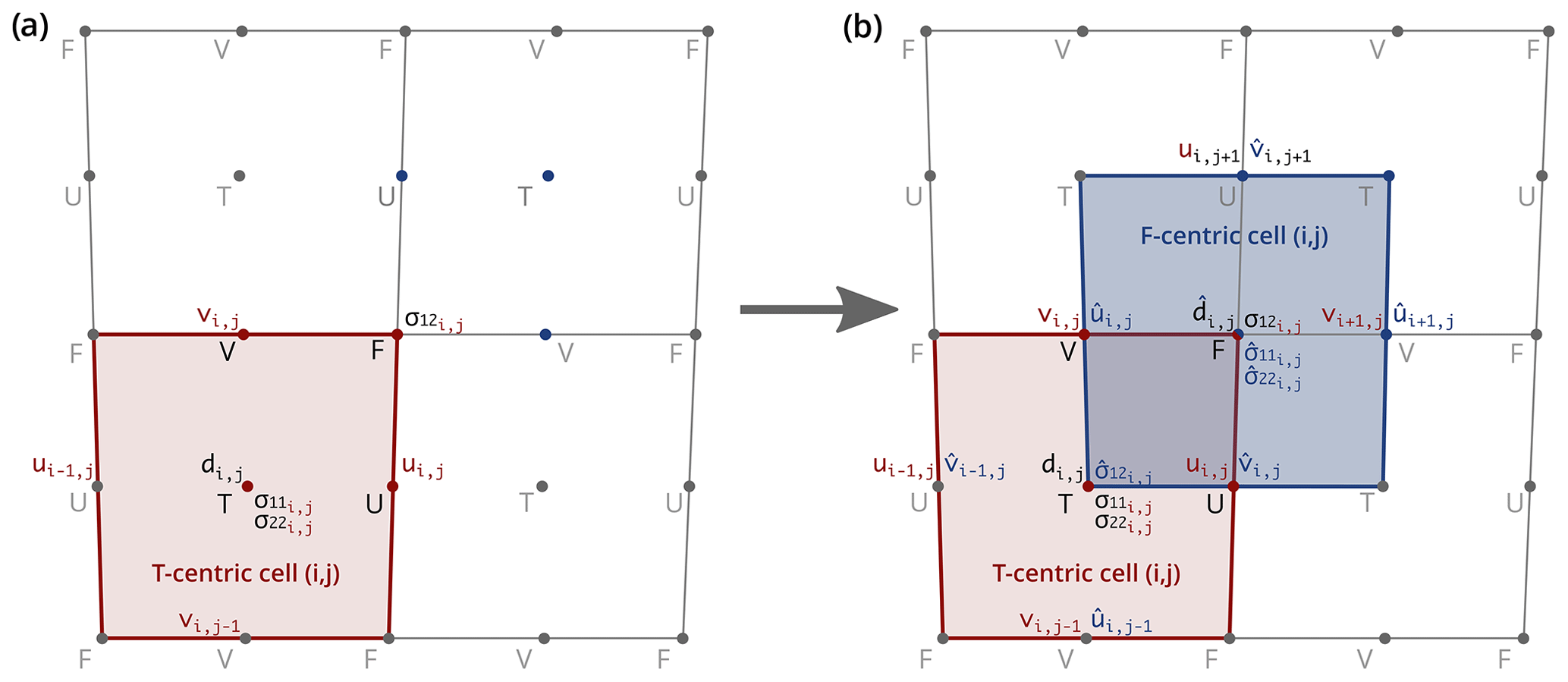
Figure 3Transition from (a) the conventional C-grid staggering as used in NEMO to (b) the E-grid staggering proposed in this study. T-centric (red) and F-centric (blue) cells. d is the damage tracer, u and v are the i- and j-wise components of the sea ice velocity vector, and σkl represents the components of the internal stress tensor. The notation indicates that variable x is specific to the F-centric grid. Note: the F-centric counterparts of ui,j and vi,j of the T-centric cell are and .
As suggested by Fig. 3b, the E-grid can be seen as a superposition of two C-grids, in which the cell center of the additional C-grid coincides with the upper-right corner of the original C-grid. For convenience, we will refer to these two grids as F-centric (additional) and T-centric (original), respectively.
In order to minimize the number of modifications and rewriting in the SI3 code, the idea was to restrict the use of this E-augmented C-grid to rheology and advection modules only. The rest of the code, which includes the thermodynamics, remains unmodified and relies entirely on the standard C-grid. As such, only rheology-specific tracers are defined in the E-grid fashion, i.e., at both T- and F-points. In our case, this applies only to the ice damage d and components of the internal stress tensor (even though components of a tensor cannot exactly be considered tracers when it comes to the advection; see Sect. 2.4). However, global tracers, such as ice concentration and thickness, which are updated within the thermodynamics module, remain defined at the T-point only. Consequently, these tracers are interpolated at the F-point within the rheology module whenever needed.
To summarize, in the proposed rheology-specific E-augmented C-grid approach, as shown in Fig. 3, the conventional C-grid model variables are augmented with (i) the u-velocity component at V-points and v-velocity component at U-points; (ii) the ice damage, σ11, and σ22 at F-points; and (iii) σ12 at T-points. This approach implies that all the equations related to the dynamics, including constitutive and momentum equations, as well as the advection, have to be solved twice: on both the T- and F-centric grids. As detailed in Appendix B, the exact same discretization and numerical schemes can be used on both grids, with only the indices of the velocity components on the F-centric grid requiring particular attention: and have to be used as the counterparts of ui,j and vi,j on the T-centric grid (Fig.3.b). This applies to the computation of the strain rate tensor (Sect. B2.1), the constitutive equation (Sect. B2.2), momentum equation (Sect. B3), the divergence of the stress tensor (Sect. B3.1), and the advection.
At this stage it is important to note that the doubling of the number of computational points implied by the transition to the E-grid in no way relates to an increase in the spatial resolution of the original C-grid. That is because the FD discretization of spatial derivatives on the E-grid (see Appendix B) still relies on the same local spatial increment, i.e., Δx, as that of the original C-grid, regardless of the subgrid considered (T- or F-centric).
2.3.2 The separation of solutions and how it is restrained
With the E-augmented C-grid approach, all rheology-specific prognostic variables are defined at the points where their value is required, and no interpolation is needed to solve the equations. It does, however, result in an apparent overdetermination, which allows the T- and F-centric solutions to evolve somewhat independently from one another. This separation of solutions rapidly degenerates into unrealistically noisy solutions as the spatial consistency of the fields between the two grids deteriorates.
This problem of grid separation has been known since the early adoption of the E-grid by the community (Arakawa, 1972; Mesinger, 1973; Janjić, 1974; Janjić and Mesinger, 1984; Mesinger and Popovic, 2010). It is mostly discussed in the context of the shallow-water equations and is often referred to as “(short) gravity wave decoupling” or “lattice separation”. Various treatments and methods have been proposed, from filtering approaches to more advanced ones such as the introduction of auxiliary velocity points midway between the neighboring tracer points (Mesinger, 1973; Janjić, 1974; Mesinger and Popovic, 2010). Interestingly, the E-grid was used in the Hamburg Large-Scale Geostrophic (LSG) model (Maier-Reimer et al., 1993) in order to achieve more accurate geostrophic balance, while retaining some advantages of the C-grid such as the straightforward discretization of the divergence. In their model, the problem of grid separation, already limited due to the use of a monthly time step, was overcome through adding horizontal viscosity and diffusion. Recently, Konor and Randall (2018) also mentioned the need to introduce a “horizontal mixing process” to avoid the “separation of solutions” when using the E-grid.
The cause of the separation of the two solutions resides in the weak coupling between the two grids, as they only exchange very little information. Specifically, in our case, the only exchange of information between the T- and F-centric grids occurs via the shear stress σ12 and the ice velocity vector. The estimate of of the T-centric grid (at F-point), based on Eq. (9), uses , , and of the F-centric grid (at F-point) and conversely for . Similarly, the correction of in Eq. (12), if occurring, uses and . For the velocity, the exchange of information occurs in the Coriolis term of Eq. (1) and through the advection of σ12 via and (and that of via u and v). As suggested by results discussed later in this section, this exchange of information is not sufficient enough to prevent the decoupling of the solutions between the two grids. Hence, a numerical treatment is required to constrain the T- and F-centric solutions to remain spatially consistent with one another.
During the early phase of our development, we considered, implemented, and tested a variety of such treatments. As of now, only one has proven able to prevent the grid separation issue without leading to noisy and/or unrealistic solutions. This treatment, which operates sequentially on the T- and F-centric stress tensors at the dynamical time step level, is hereafter referred to as cross-nudging (CN). It consists of nudging each vertically integrated component of the T-centric stress tensor (σ) towards its F-centric counterpart () interpolated at the relevant point under even time step integrations and conversely under odd time step integrations. This is written as follows:
where γcn is the CN coefficient, Ns is the time-splitting parameter (Eq. 15), the bar notation denotes the spatial interpolation from F- to T-points or T- to F-points (see Eq. A1 in Appendix A3), and stress components in bold are vertically integrated (Appendix A4). Each of the two tensors is “corrected” times during the course of one advective time step ΔT. The form of the term that modulates the nudging intensity, i.e., , ensures that the level of cross-nudging undergone by the two tensors under one ΔT is primarily controlled by γcn and remains somewhat independent of the choice of Ns.
Due to the strong damage–stress interdependence (Sect. 2.2), the CN is applied to σ(i) rather than σ, i.e., after solving the constitutive equation (Eq. 9) but before computing dcrit and applying the stress correction (Eq. 12). Applying the CN after the stress correction stage (rather than before) may result in the use of a mix of (i) stress values that have been corrected through a local increase in damage and (ii) uncorrected stress values (with no increase in damage). This may lead to spatial inconsistencies between the post-CN stresses and the damage field.
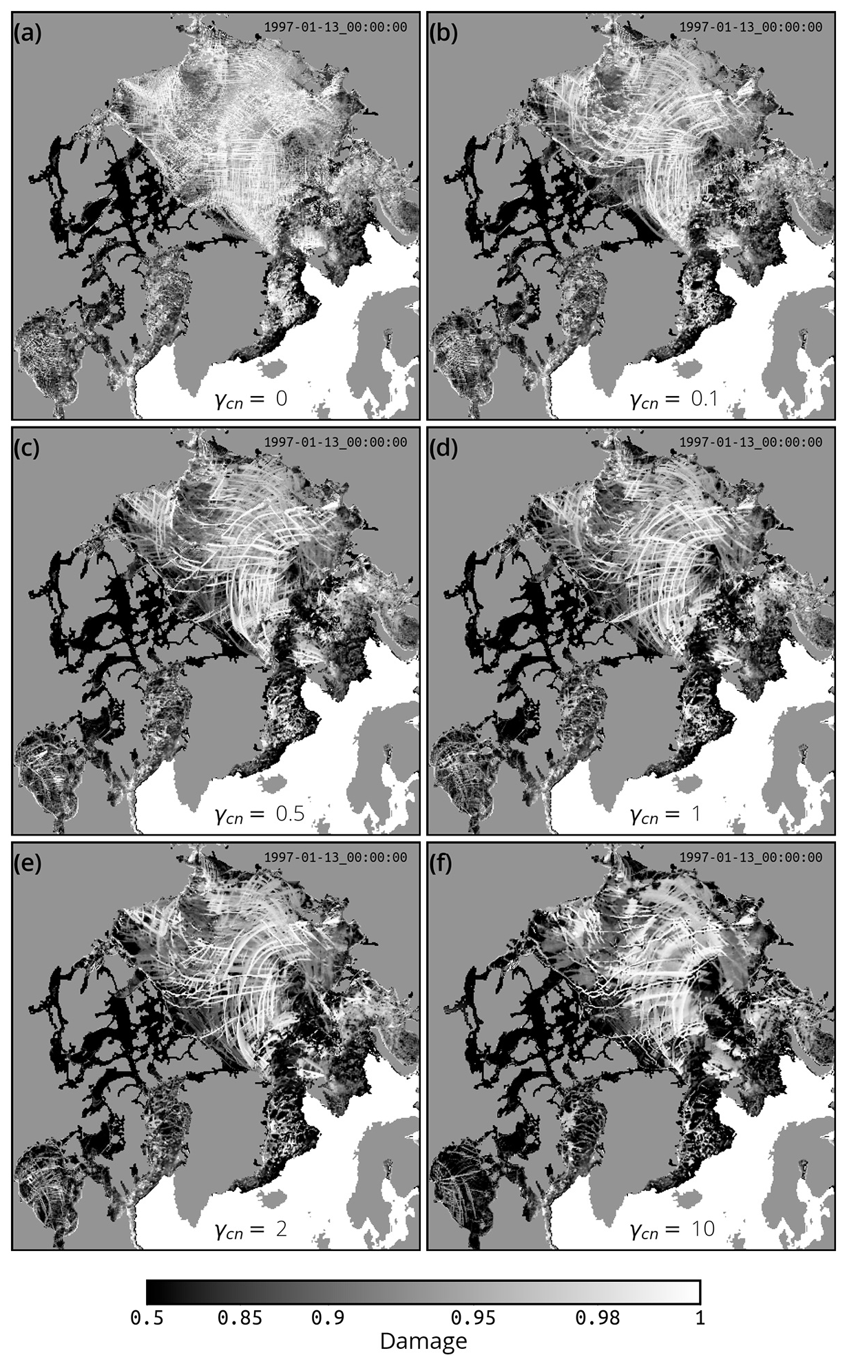
Figure 4Effect of using different values for the cross-nudging coefficient γcn on the simulated sea ice damage. Random snapshot of damage (at T-points, 13 January 1997) after 30 d of simulation using the specified value of γcn in a set of sensitivity experiments identical to SI3-BBM: (a) no cross-nudging, (b) γcn=0.1, (c) γcn=0.5, (d) γcn=1 as in SI3-BBM, (e) γcn=2, and (f) γcn=10.
The four-point spatial averaging (interpolation) used in the CN inevitably results in the introduction of a smoothing of the solution in space. As such, γcn is chosen to achieve the best compromise between the smoothing and the coupling of the T- and F-centric solutions. We have performed sensitivity tests with our pan-Arctic setup and we conclude, relying exclusively on the visual assessment of the simulated fields, that the right compromise is achieved when γcn is typically of the order of 1, with γcn=1 being the value used in our experiments. As illustrated in Fig. 4, with a value below 1, the solutions become increasingly noisy as γcn approaches zero. In particular, the damage field tends to exhibit strongly unrealistic straight-line features of high damage that are aligned along the x or y axis of the grid. Our results suggest that values of γcn typically above 2 lead to an excessive smoothing of the solutions (as shown, for example, for γcn=10 in Fig. 4f). The value of γcn appropriate for a given model setup is likely to be dependent on different factors that we have not identified yet. As such, we can only recommend that potential users of our implementation consider γcn a tuning parameter that should be adjusted for a given setup. However, simulations that we have performed at spatial resolutions of 1, 2, 4, and 10 km with the idealized test case discussed in Sect. 3.1 (not shown) suggest that γcn is only weakly influenced by the spatial resolution at which the model is run (values typically between 0.5 and 2 consistently yielding what we refer to as the best compromise).
2.4 Horizontal advection
In neXtSIM, the Lagrangian finite-element model used by Ólason et al. (2022), the advection occurs implicitly at each advective time step (also corresponding to the thermodynamics time step) through the ice-velocity-driven displacement of the mesh elements. As such, the rate of change of a prognostic scalar ϕ is . In the present Eulerian context, however, the term relative to the horizontal advection has to be considered so that the rate of change of ϕ is now . In our implementation, as pointed out by Ólason et al. (2022), this advection term is computed and added to the trend of the prognostic scalar considered every advective time step. Thus, the sea ice velocity vectors U and V that we consider for the advection at the advective time step level represent the mean of the Ns successive velocity vectors (u and v) calculated under one time-splitting instance.
We use the second-order moment (SOM) advection scheme of Prather (1986) available in SI3 to advect the damage and the components of the stress tensors (considered to be scalars for now; see Sect. 2.4.1). Technically, the damage and stress tensor components defined at the T-point (d, σ11, σ22, and ) are advected using U and V defined at U- and V-points, respectively. Their F-point counterparts (, , , and σ12) are advected using and defined at V- and U-points, respectively. In practice, the exact same implementation of the advection scheme can be used to perform the advection at T- and F-points; the only difference is that for the advection of F-point scalars, the spatial indexing of the velocity components is staggered by one cell. Namely, and have to be used in place of Ui,j and Vi,j (Fig. 3b).
As it is commonly done in sea ice models and justified by a scale analysis of the momentum equation, the term for the advection of momentum is neglected.
2.4.1 Advection of the internal stress tensor
In the Eulerian framework, the rate of change of a second-rank tensor must introduce additional terms to the material time derivative in order for the dynamics of the tensor to remain independent of the frame of reference (Oldroyd, 1950; Larson, 1988; Hinch and Harlen, 2021; Stone et al., 2023). These terms account for the effects of rotation and deformation of the medium on the evolution of the stress tensor and are gathered here in a symmetric tensor :
As stressed by Snoeijer et al. (2020), one faces a “a somewhat unpleasant ambiguity” as two different formulations exist for . Both formulations are equally valid in terms of frame invariance, and so is any linear combination of the two. The first formulation is the upper-convected time derivative of σ, denoted as ,
which, in component form, simplifies into
The second formulation is the lower-convected time derivative, denoted as ,
with
These formulations of are straightforward to implement in the model as they only involve multiplications between the components of tensors and σ, which are all defined at both T- and F-points with the E-grid. Therefore, we have implemented both formulations in SI3. In our implementation, the standard advection trend for each tensor component, corresponding to the term (U⋅∇) σ in Eq. (17), is computed using the identical scheme to that used for regular scalar fields. The tensor-specific advection trend, , is computed according to Eq. (19) or (21). These two contributions are computed independently from one another using stress values that have not been updated yet by the advection process.
We have chosen to use the upper-convected formulation in both the idealized and pan-Arctic simulations presented in this paper. This choice is purely arbitrary and is not based on scientific considerations of any kind. It relies solely on the fact that the upper-convected formulation has been favored in the literature since Oldroyd, who introduced both formulations in his 1950 paper, found that his model would only realistically represent the flow around a rotating rod when using this formulation, as opposed to the lower-convected one (Hinch and Harlen, 2021). Nevertheless, two twin simulations of our reference BBM simulation (see Sect. 3.2) have been run, one using the traditional material derivative (i.e., ) and the second the lower-convected formulation. All the diagnostics and deformation statistics discussed later in this paper have been performed for these two additional simulations and no significant differences have been identified among the three options (PDFs of the total deformation for the reference and additional simulations are provided in Fig. C3 in Appendix C as an example).
Further work, involving, for example, the design of new idealized test cases, should be conducted to address this ambivalence and help identify which time-derivative formulation (or combination of them, such as the Gordon–Schowalter time-derivative discussed by Dansereau et al., 2016) is best adapted to sea ice rheology.
2.5 Construction of observed and simulated Lagrangian sea ice deformations
Our assessment of the NEMO pan-Arctic simulations relies on a multiscale statistical analysis of sea ice deformation rates constructed using observed and simulated Lagrangian sea ice trajectories during winter 1996–1997. Observed trajectories are taken from the RGPS (RADARSAT Geophysical Processor System Lagrangian trajectories) dataset of Kwok et al. (1998), while simulated trajectories are generated from the Eulerian sea ice velocities of SI3 by means of a sea ice particle tracker program.
The preprocessing and computing approach we use to construct sea ice deformations out of the raw RGPS Lagrangian trajectories is very similar to that used by Ólason et al. (2022), the main difference being that it relies on the tracking of quadrangles rather than triangles. To construct the SI3-derived synthetic version of these deformations, the tracking software seeds the identical points to those involved in the definition of the quadrangles selected for computing the RGPS deformation, respecting their initial position in space and time. These points are then tracked for about 3 d using the hourly averaged Eulerian sea ice velocities of SI3; the exact tracking duration used is that of the time interval between the two consecutive positions of the corresponding RGPS point.
Our period of interest, spanning 15 December 1996 to 20 April 1997, is divided into 3 d bins, which correspond to the nominal time resolution of the RGPS dataset.
2.5.1 Selection of RGPS trajectories
For each 3 d bin, an initial subset of the RGPS points is selected. Each point of this initial subset must satisfy the following requirements:
-
The point has at least one position that occurs within the time interval of the bin; this position, or the earliest-occurring one if there is more than one occurrence, is selected and referred to as position no. 1.
-
Position no. 1 is located at least 100 km away from the nearest coastline.
-
The point has at least one upcoming position that occurs 3 d after position no. 1, with a tolerated deviation of ± 6 h, referred to as position no. 2 (in the event of more than one position satisfying this requirement, the position yielding the time interval the closest to 3 d is selected).
2.5.2 Quadrangulation of selected trajectories
A Delaunay triangulation is performed on this initial subset of points at position no. 1. Triangles whose areas differ by more than 25 % from the half of the nominal area of the quadrangles to be constructed (i.e., the square of the spatial scale under consideration) or with an angle below 5° or above 160° are excluded. Neighboring pairs of remaining triangles are then merged into quadrangles in order to transform the triangular mesh into a quadrangular mesh.
Aspiring quadrangles at position no. 2 are constructed by simply considering the exact same respective sets of four points as those defining quadrangles at position no. 1.
Finally, only points that define quadrangles that satisfy the following requirements at both position no. 1 and position no. 2 are retained:
-
The square root of the area of the quadrangle falls within a ± 12.5 % range of agreement with the horizontal scale under consideration.
-
The time position of each of the four points defining the vertices of the quadrangle should not differ from that of any of the other three points by more than 60 s.
-
The thresholds for the minimum and maximum angles allowed are 40 and 140°, respectively.
2.5.3 Computation of deformation rates based on the quadrangles
For all quadrangles selected in a given 3 d bin, strain rates are computed based on their position no. 1 and no. 2 using the line-integral approximations (see, e.g., Lindsay and Stern, 2003, Eqs. 10–14).
The time location (date) assigned to a given deformation rate corresponds to the center of the time interval defined by position no. 1 and position no. 2 of each quadrangle. The spatial location of the deformation rates corresponds to the barycenter of the four vertices of the quadrangle considered at the center of this same time interval.
2.5.4 Construction of the simulated Lagrangian sea ice trajectories
To save computer resources, only the points from which valid RGPS deformation estimates were computed are retained. Each of these points is seeded using the same initialization date and location (bilinear interpolation) as its RGPS counterpart. It is then tracked during the same time interval of about 3 d (± 6 h) that separates the two consecutive records of the RGPS point considered. The tracking software uses a time step of 1 h and feeds on the hourly averaged simulated sea ice velocities of the SI3 experiments. Note that only the conventional C-grid velocities u and v of the T-centric cell are used to track the points ( and , available in the BBM-driven simulation, are not used).
We use version 4.2.2 of the NEMO modeling system (Madec et al., 2022) as the basis for the development of the BBM rheology code extension and to perform both the idealized and coupled pan-Arctic simulations to be assessed. Since version 4, the default sea ice component of NEMO has been SI3 (Vancoppenolle et al., 2023).
3.1 Idealized simulations
To provide a first qualitative evaluation of the behavior of our BBM implementation, SI3 simulations were run on the idealized test case setup introduced by Mehlmann et al. (2021), including simulations using the default aEVP-driven SI3 setup for reference purposes. This test case, defined on a 512 km wide square domain, simulates a cyclone traveling in the northeastward direction over a thin layer of ice (h ≃ 0.3 m) that floats on an anticyclonically circulating ocean. This test case is well suited to illustrate the influence of the grid discretization on rheology-related processes such as the representation of linear kinematic features (LKFs) (Danilov et al., 2022, 2024), which makes it particularly relevant to our study. We use the identical setup and parameter values to those defined in Mehlmann et al. (2021) (see the “Code and data availability” section to access the SI3 namelists and forcing files). SI3 is run in stand-alone mode using SAS, the stand-alone surface module of NEMO. In SAS mode, SI3 uses a prescribed surface ocean state (current, height, temperature, and salinity) instead of being coupled to the ocean component of NEMO as in our pan-Arctic simulations (Sect. 3.2).
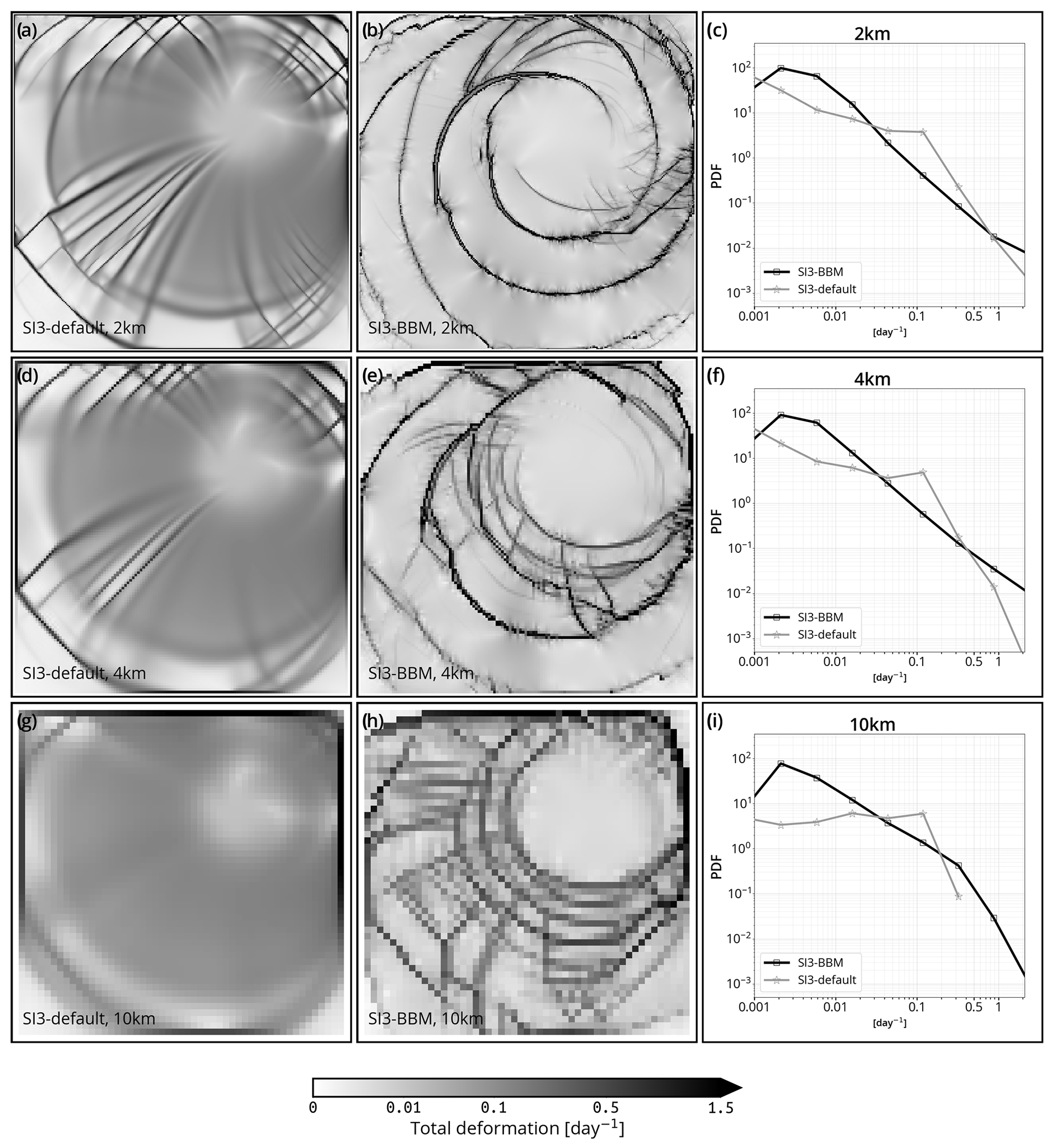
Figure 5Sea ice total deformation (instantaneous) in the test case described by Mehlmann et al. (2021) after 48 h of simulation with SI3 using the default SI3 aEVP setup and the newly implemented BBM rheology (left-hand and middle column, respectively) and the corresponding PDFs (right-hand column) for simulations run at a spatial resolution of 2, 4, and 10 km (first, second, and third row, respectively).
The results of this test case, for both the aEVP and BBM rheology, are shown in Fig. 5. First we note that for the SI3 implementation of aEVP, the deformation fields obtained are in qualitative agreement with those of Mehlmann et al. (2021) (see, for instance, their Fig. 7). In the solutions obtained with BBM, we note the presence of a circular network of LKFs that contrast, by their arrangement, with the “spider-web-like” arrangement of the LKFs in the aEVP solution. In the BBM-driven simulation these LKFs are also simulated in the 10 km setup (Fig. 5h). The spatial pattern of the LKFs, particularly those accommodating the highest deformation, also look qualitatively different: apparently longer and with circular and concentric shapes with respect to the center of the forcing cyclone in the case of BBM, shorter and in radial alignment with respect to the forcing cyclone in the aEVP case.
We also find that the background deformation field is close to zero in the BBM solution, except along the LKFs, whereas the deformation looks more homogeneous in space in the aEVP solution. This can also be seen on the respective PDFs (Fig. 5c, f, and i) that exhibit different shapes and heavier tails in the BBM solution. We have verified that the aEVP solution is not too significantly impacted by the number of iterations used in the aEVP solver of SI3 by conducting the same aEVP experiments with a NEVP = 1000 instead of NEVP = 100 (Fig. C1).
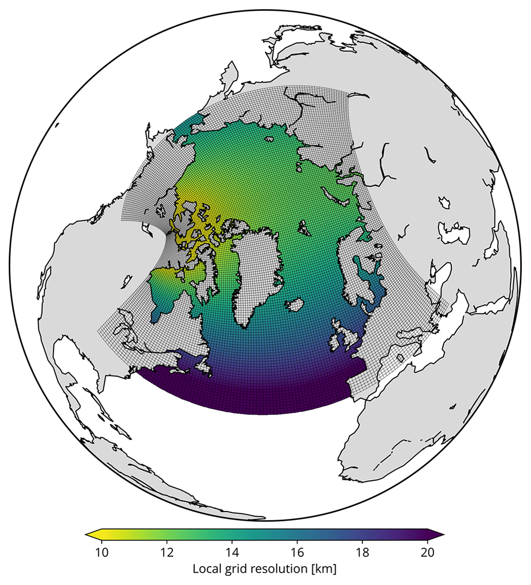
Figure 6Geographical extent, numerical grid, and actual local spatial resolution of the NANUK4 computational domain that is used in the experiments. For ease of visual representation of the grid cells, grid points have been subsampled by a factor of 4.
Finally, we note that the solutions do not contain any apparent numerical instabilities or noise for aEVP or BBM. The LKF-like features in the BBM solution at 10 km show a tendency to align horizontally, vertically, and diagonally with the grid. As of now, we are unable to provide an explanation of the mechanism responsible for these alignments, apart from their apparent connection with the use of a relatively coarse spatial resolution, as the solution obtained with the 4 km setup seems to be rid of them.
3.2 Coupled ocean–sea ice pan-Arctic simulations
The pan-Arctic simulations use SI3 coupled to the 3D ocean component of NEMO, named OCE. They are performed on the so-called NANUK4 regional configuration, which is an Arctic extraction of the standard global ° resolution NEMO gridded horizontal domain known as ORCA025 (Barnier et al., 2006). As such, and as shown in Fig. 6, the actual grid resolution of NANUK4 typically spans 10 up to 14 km in the central Arctic region. NANUK4 features two open lateral boundaries; the southernmost boundary is located at about 39° N in the Atlantic Ocean, and the second boundary is located south of the Bering Strait, at about 62° N in the Pacific Ocean. The vertical z-coordinate grid used for the ocean features 31 levels with a Δz of 10 m at the surface up to about 500 m at the deepest level, at a depth of 5250 m.
The hindcast nature of the simulations is achieved through the use of interannual atmospheric and oceanic forcings at the surface and at the two open boundaries, respectively. For the atmospheric forcing, both the ocean and the sea ice components receive, as surface boundary conditions, fluxes of momentum, heat, and fresh water at the air–sea and air–ice interface, respectively. These fluxes are computed every hour by means of bulk formulae using the hourly near-surface atmospheric state from the ERA5 reanalysis of the ECMWF (Hersbach et al., 2020) and the prognostic surface temperature of the relevant component (SST or ice surface temperature).
For the lateral boundary conditions of OCE, the 3D ocean is relaxed towards the monthly averaged 3D horizontal velocities, temperature, salinity, and SSH (2D) of the GLORYS2v4 ocean reanalysis (Ferry et al., 2012).
Table 1Values of default aEVP-related parameters in SI3, as used in experiment SI3-default.
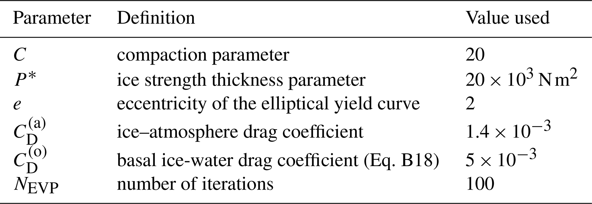
Table 2Values of BBM-related parameters implemented in SI3, as used in experiment SI3-BBM.
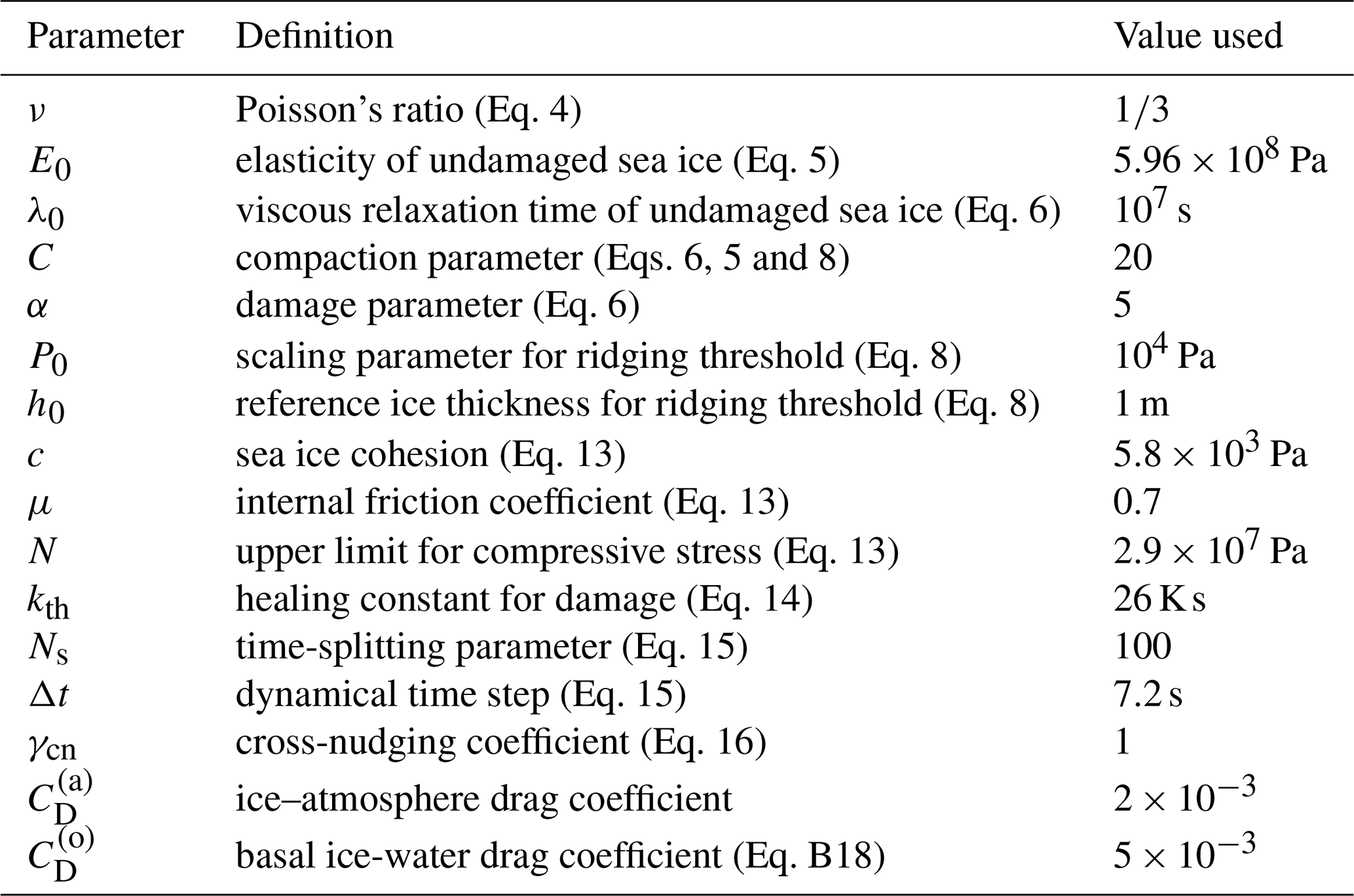
Both OCE and SI3 use a time step of ΔT = 720 s, the advective time step. The coupling between these two components is also done at each advective time step. Our control simulation, named SI3-default, uses the default SI3 setup as provided in NEMO and thereby uses the aEVP rheology of Kimmritz et al. (2016). The second simulation, named SI3-BBM, only differs from SI3-default through the use of our implementation of the BBM rheology in place of aEVP and a higher value of the air–ice drag coefficient. Values of parameters relevant to both rheologies used in the two simulations are provided in Tables 1 and 2, respectively.
The two simulations are initialized on 1 December 1996 using the same restart data generated at the end of a 2-month spin-up performed with the SI3-default setup and run until 20 April 1997. This spin-up is initialized on 1 October 1996 by using the daily averaged ocean and sea ice data from the GLORYS2v4 reanalysis as an initial condition. More specifically, OCE is initialized at rest (no current) with the 3D temperature and salinity state of the reanalysis, while SI3 is initialized with the sea ice concentration and thickness. The 2-month spin-up we use is long enough to get the ocean velocities in the upper ocean into a good state with the given temperature and salinity fields. Our strategy implies that SI3-BBM is initialized on 1 December 1996, with a value of ice damage set to zero everywhere, which poses no issue as the time required to spin up the damage is very short (Bouillon and Rampal, 2015; Rampal et al., 2016), typically of the order of a few days. The analysis of the results is performed for the period 15 December 1996–20 April 1997, leaving the upper ocean and the sea ice cover in SI3-BBM 2 weeks to respond to the changed rheology, which should be ample.
For these simulations, the adjustable tuning parameters of SI3 are kept as close as possible to those of the reference configuration of NEMO (Tables 1 and 2). As such, the thermodynamic component uses five ice categories. Yet, the ice–atmosphere drag coefficient has been adjusted from 1.4 × 10⁻³ to 2 × 10⁻³ in SI3-BBM in order for the mean simulated deformation rate at the 10 km scale to be in agreement with that derived from the satellite observations against which we evaluate the model (see Sects. 2.5 and 3.3.3). In SI3-default, the default value of 1.4 × 10⁻³ satisfies this requirement and is left unchanged. For the time-splitting approach (Sect. 2.2), we use a dynamical time step of 7.2 s in SI3-BBM, which relates to a time-splitting parameter of Ns=100.
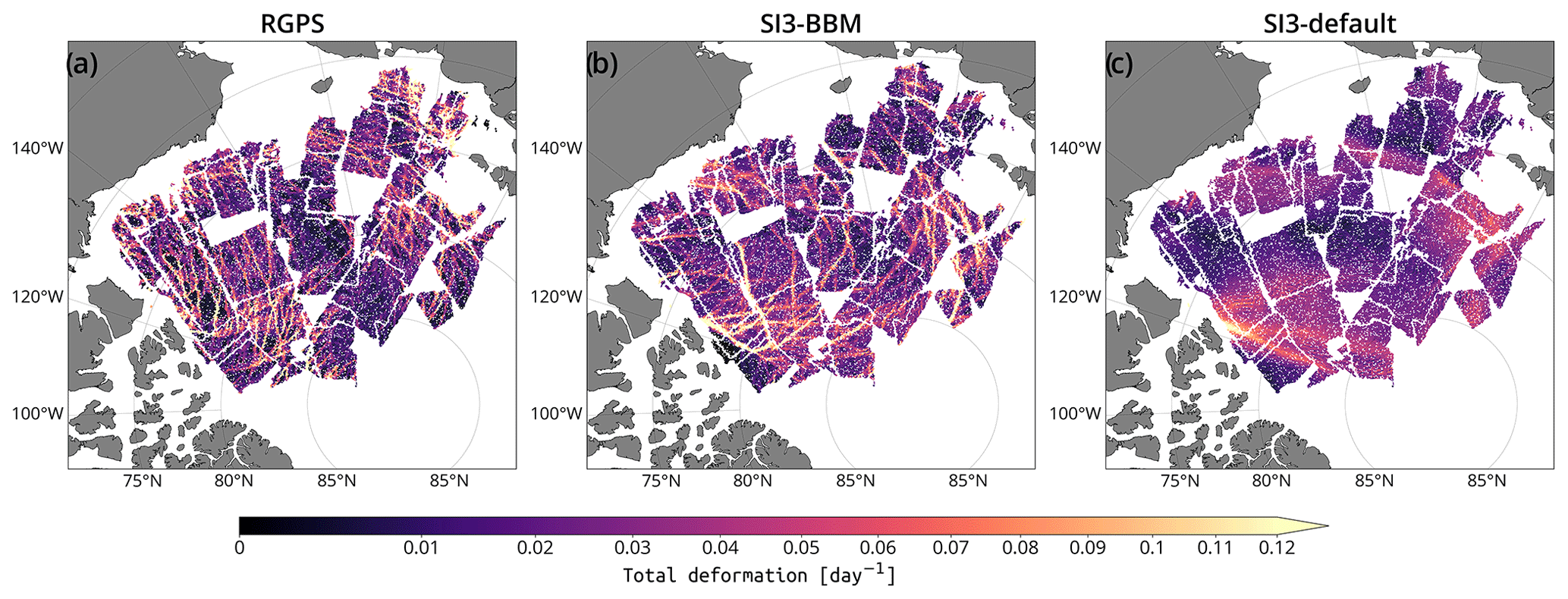
Figure 7Maps of the sea ice total deformation rate at the 10 km spatial and 3 d temporal scale for the period centered about 24 December 1996, computed based on (a) RGPS Lagrangian data and (b, c) their synthetic counterparts constructed using the simulated sea ice velocities of SI3-BBM and SI3-default, respectively. Empty regions correspond to the absence of satellite data during the period concerned.
3.3 Comparison of simulated sea ice deformation statistics against satellite data
3.3.1 Probability density function of sea ice deformation rates
As illustrated by the maps of the 3 d total deformation rates (Fig. 7), RGPS clearly exhibits narrow and long features, commonly called linear kinematic features (LKFs; Kwok, 2001) along which the deformation is concentrated. Visually, LKFs simulated by SI3-BBM appear somewhat realistic in terms of both length and orientation, and the magnitude of the deformation rates along these LKFs is similar to that of RGPS. We note that SI3-default exhibits very smooth fields of deformation with almost no such localized features; this is consistent with the findings of recent studies that evaluate VP-driven sea ice simulations run at a grid resolution typically coarser than 5 km (e.g., Ólason et al., 2022; Bouchat et al., 2022).
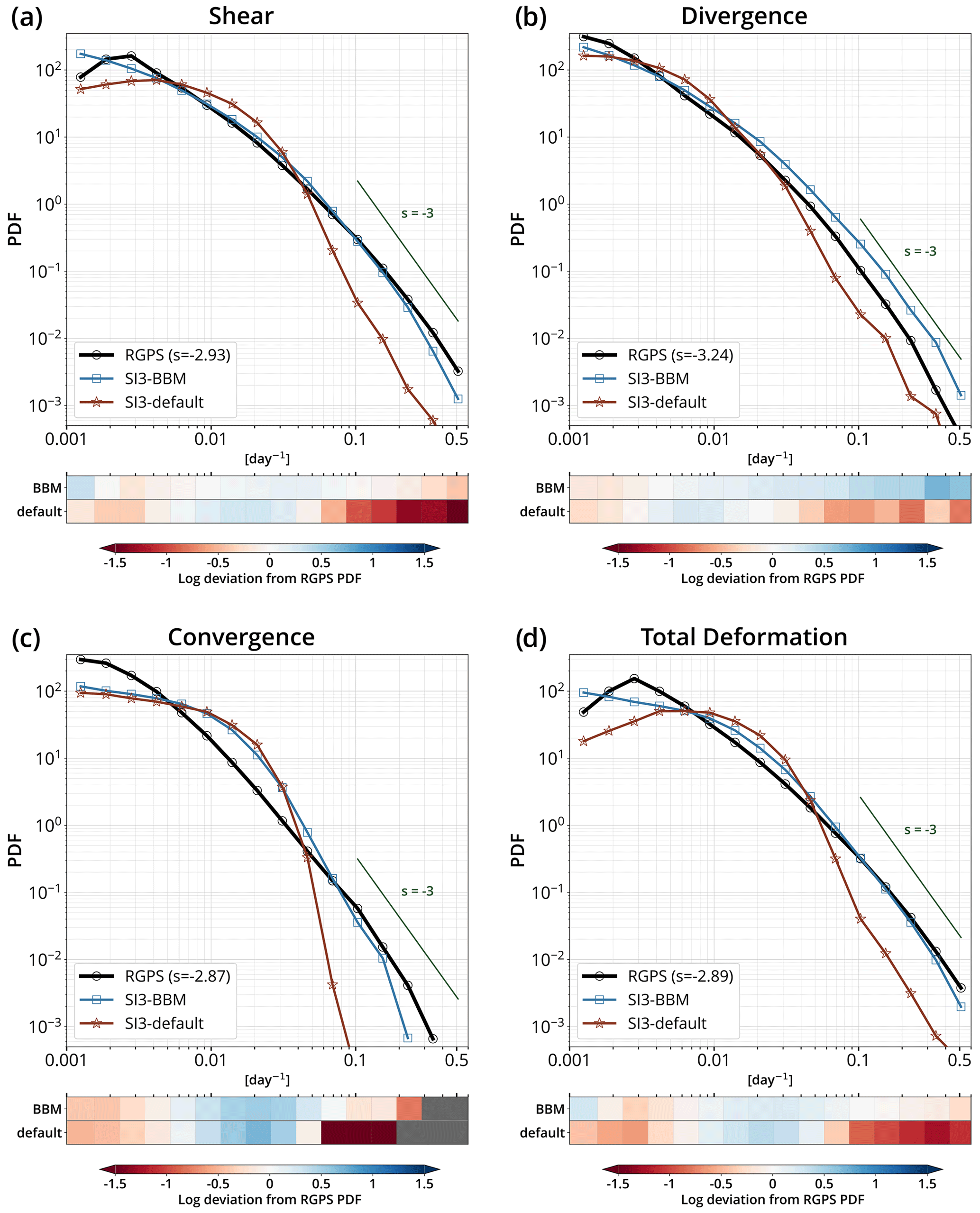
Figure 8PDFs of the (a) shear, (b) divergence, (c) convergence, and (d) total deformation rates at the 10 km spatial and 3 d temporal scale for RGPS data and their synthetic counterparts constructed using the simulated sea ice velocities of SI3-BBM and SI3-default. The light gray lines are for reference and correspond to a power law with an exponent of −3. Below each panel, the departure between the logarithm of the simulated and observed distributions is shown for each bin.
The PDFs of the total deformation rates (Fig. 8d) show that SI3-BBM exhibits a heavy tail similar to that of RGPS and that it can be approximated by a power law over the values corresponding to the last two percentiles of the RGPS distribution, although with slightly different exponents (−2.9 and −3, respectively). A look at the other invariants of the deformation (i.e., shear, divergence, and convergence rates in Fig. 8a–c) shows that SI3-BBM simulates large deformation events as seen in the observations, which suggests the ability of BBM to capture the heterogeneous character of sea ice deformation in this setup. In contrast, SI3-BBM is unable to reproduce the observed convergence over the full range of values present in the RGPS data (Fig. 8c). This limitation of the BBM rheology is further discussed in Sect. 4.2.
Our results suggest a propensity for SI3-default to underestimate the extreme values of deformation rates. This inadequacy of the model could very likely be mitigated by conducting a finer tuning of the parameters related to the viscous–plastic rheology, in particular through the better adjustment of the ratio between the ice compressive strength and the ice shear strength (Bouchat and Tremblay, 2017). Yet, conducting such a tuning is out of the scope of this paper. Interestingly, the underestimation of extreme deformation values set aside, SI3-default exhibits a power-law behavior similar to that of both observations and SI3-BBM, with similar exponents, except in convergence.
3.3.2 Time series of sea ice deformation rates
Following Ólason et al. (2022), we examine the 90th percentile of the total deformation (P90), chosen for its sensitivity to the high values that contribute to shaping the long tail of the PDFs of deformations. Technically, P90 is the value of deformation below which 90 % of deformation values in the frequency distribution fall. P90 is computed from each snapshot of deformation from mid-December 1996 to late April 1997 to evaluate the temporal evolution of the deformation. In addition to the 90th percentile, we also consider the 95th and 98th percentiles.
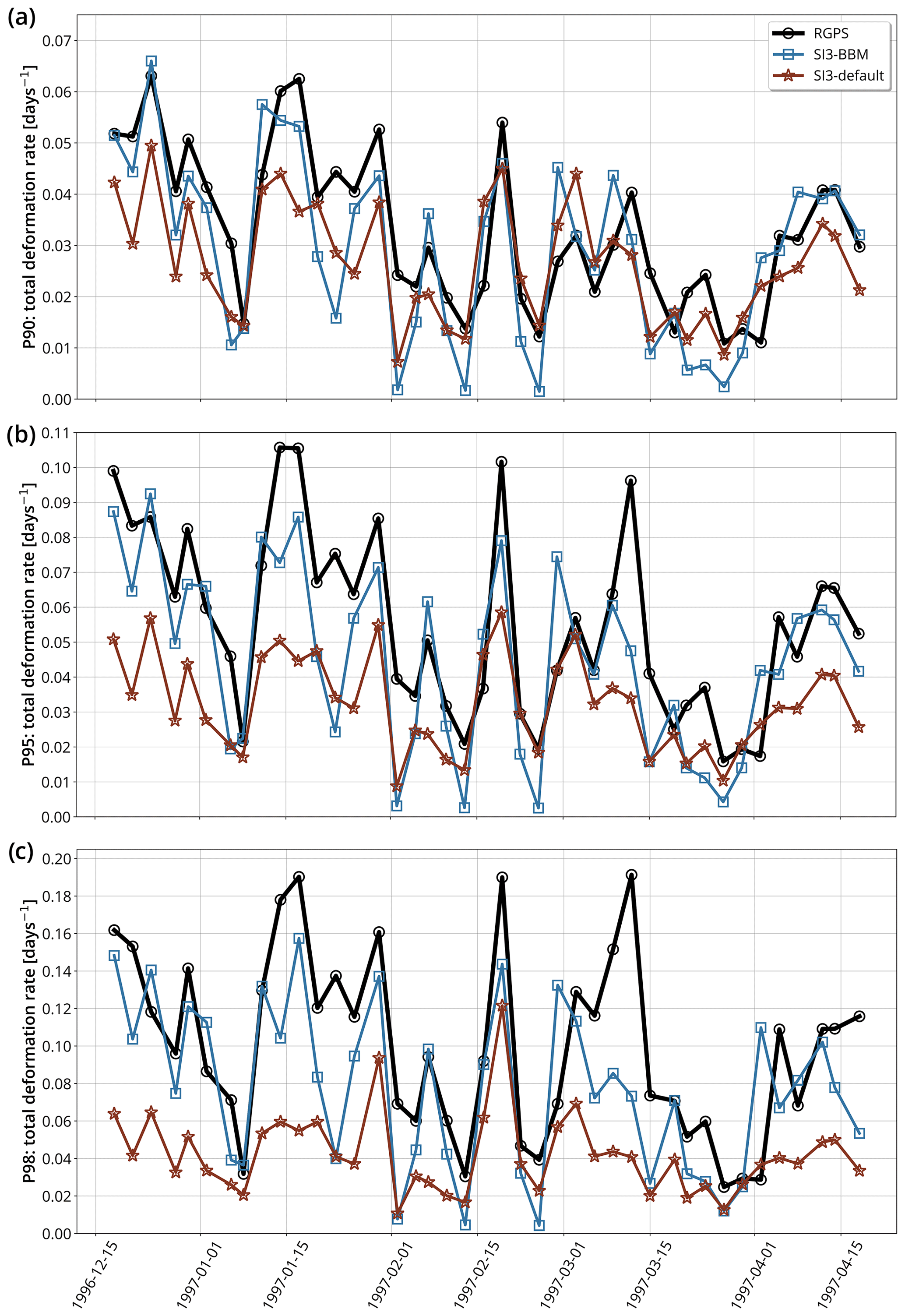
Figure 9Time series of the (a) 90th, (b) 95th, and (c) 98th percentiles of the sea ice total deformation rate for winter 1996–1997 at the 10 km spatial and 3 d temporal scale for RGPS data and their synthetic counterparts constructed using the simulated sea ice velocities of SI3-BBM and SI3-default.
As illustrated in Fig. 9, SI3-BBM is in fairly good agreement with the observations, in particular for the P90 values (see Table 3). We note, however, that despite the ability of SI3-BBM to reproduce a variability similar to that observed, the higher the percentile value, the lower the agreement between the magnitudes. This suggests an inability of the BBM rheology to capture the most extreme deformation events.
Table 3Bias, RMSE, and Pearson correlation of the deformation rate time series in Fig. 9 obtained between each simulation and RGPS.
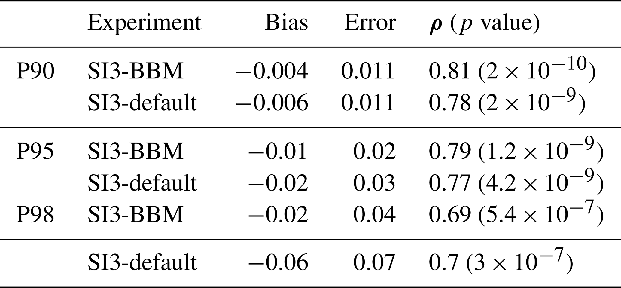
We note that the biases and RMSEs are very similar between the two simulations. For P90 and P95, the values suggest fairly good agreement between the two simulations and the observations. The values for P98, however, highlight the inability of both models to reproduce extreme deformation events. This is in qualitative agreement with what Ólason et al. (2022) already reported. Yet, further investigation remains necessary to assess whether this is inherent to the BBM model or could be improved through the better adjustment of the rheological parameters.
3.3.3 Multi-fractal scaling analysis
The presence of heavy tails in the distributions shown in Fig 8 implies that one needs to consider higher moments than the mean to fully describe the statistics of the sea ice deformation (Sornette, 2006). Following Marsan et al. (2004), our multi-fractal scaling analysis should be restricted to the consideration of moments of order q > 0 because zero values exist in the deformation field. Moments of order q> 3 should also be disregarded because a transition occurs typically between qc = 2.5 and qc = 3 (Schertzer and Lovejoy, 1987). This is a consequence of the tails of the distributions for RGPS and SI3-BBM being well represented by a power law with an exponent of about −3, which would cause moments of order q>qc to diverge (Savage, 1954).
We performed a multi-fractal spatial scaling analysis of the RGPS total deformation rates and their simulated counterparts, considering the moments q=1, 2, and 3 of the distributions. Both the observed and simulated statistics (mean, variance, and skewness) follow power laws (Fig. 10). In particular, the observed mean sea ice deformation rate is particularly well reproduced in SI3-BBM across the full range of spatial scales considered for this analysis and can be approximated by a power-law scaling, i.e., , where L is the spatial scale and β an exponent of about 0.15. We note that the atmospheric drag coefficient was used as the adjustment parameter in SI3 (Sect. 3.2), which led to the use of = 2 × 10⁻³ in SI3-BBM, while the = 1.4 × 10⁻³ used in SI3-default did not require any adjustment. Consistent with the results previously discussed, the higher moments, which characterize the largest and most extreme values of the distributions, remain underestimated in SI3-BBM compared to that derived from the observations. Indeed, the exponents of the power law that fits the SI3-BBM data (β = −0.6 and −1.34 for q = 2 and 3, respectively) are lower than those derived from RGPS data (β = −0.7 and −1.52). This indicates that SI3-BBM is not fully capturing the strength of the spatial scaling of sea ice deformation revealed by the observations or, in other words, that it fails to achieve the extremely high degree of spatial localization of the LKFs in the observations. Figure 10 suggests that the total deformation rates simulated by SI3-default cease to follow the expected power law for scales larger than 100 km. This is in line with published results (e.g., Hutter et al., 2018; Bouchat et al., 2022). Hutter et al. (2018) argue that the VP model needs approximately 10 grid cells to be able to resolve features, which suggests that the “effective resolution” of the model is 10 times coarser than that of the numerical grid on which it is run. This implies that one should instead consider fitting the deformation rates at a resolution 10 times coarser than that used by the model, i.e., 130 km in our case. This would yield power-law slopes that are in better agreement with those derived from observations. We argue that since sea ice deformation is a scale-invariant process at the geophysical scale, a sea ice model should be able to represent this scaling down to the model grid cell. Figure 10 suggests that our BBM implementation allows SI3 to achieve this despite the use of the Eulerian framework.
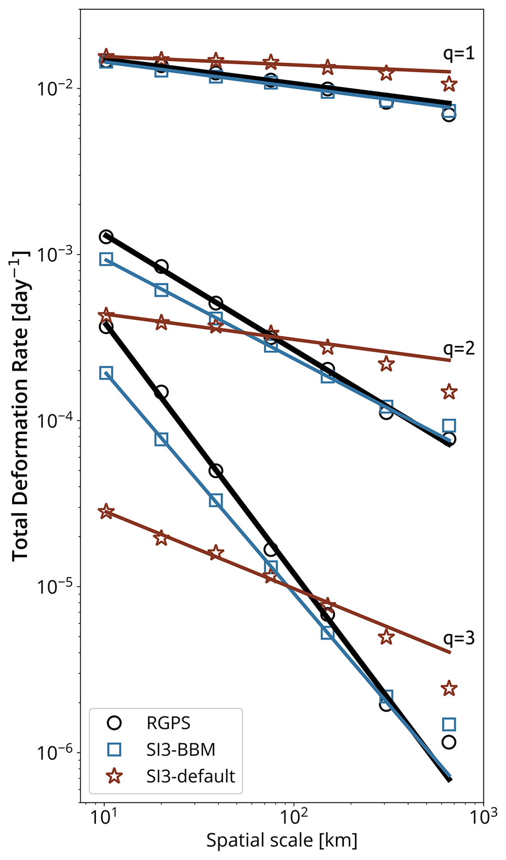
Figure 10Spatial scaling analysis of the observed and simulated total deformation rate calculated over a 3 d timescale (all based on the motion of the same RGPS quadrangles) based on RGPS data and their synthetic counterparts constructed using the simulated sea ice velocities of SI3-BBM and SI3-default. Moments of order of the distributions of the total deformation rate were calculated at scales spanning from 10 up to 640 km. The solid straight lines indicate the associated power-law scaling based on the least-square fit using values from 10 to 160 km. Values for 320 and 640 km are excluded due to excessive uncertainty resulting from the small sample size. Note: we used logarithmically spaced bins and applied an ordinary least-square method to the binned data in log–log space to get a reasonably accurate estimate of these power-law fits (Stern et al., 2018).
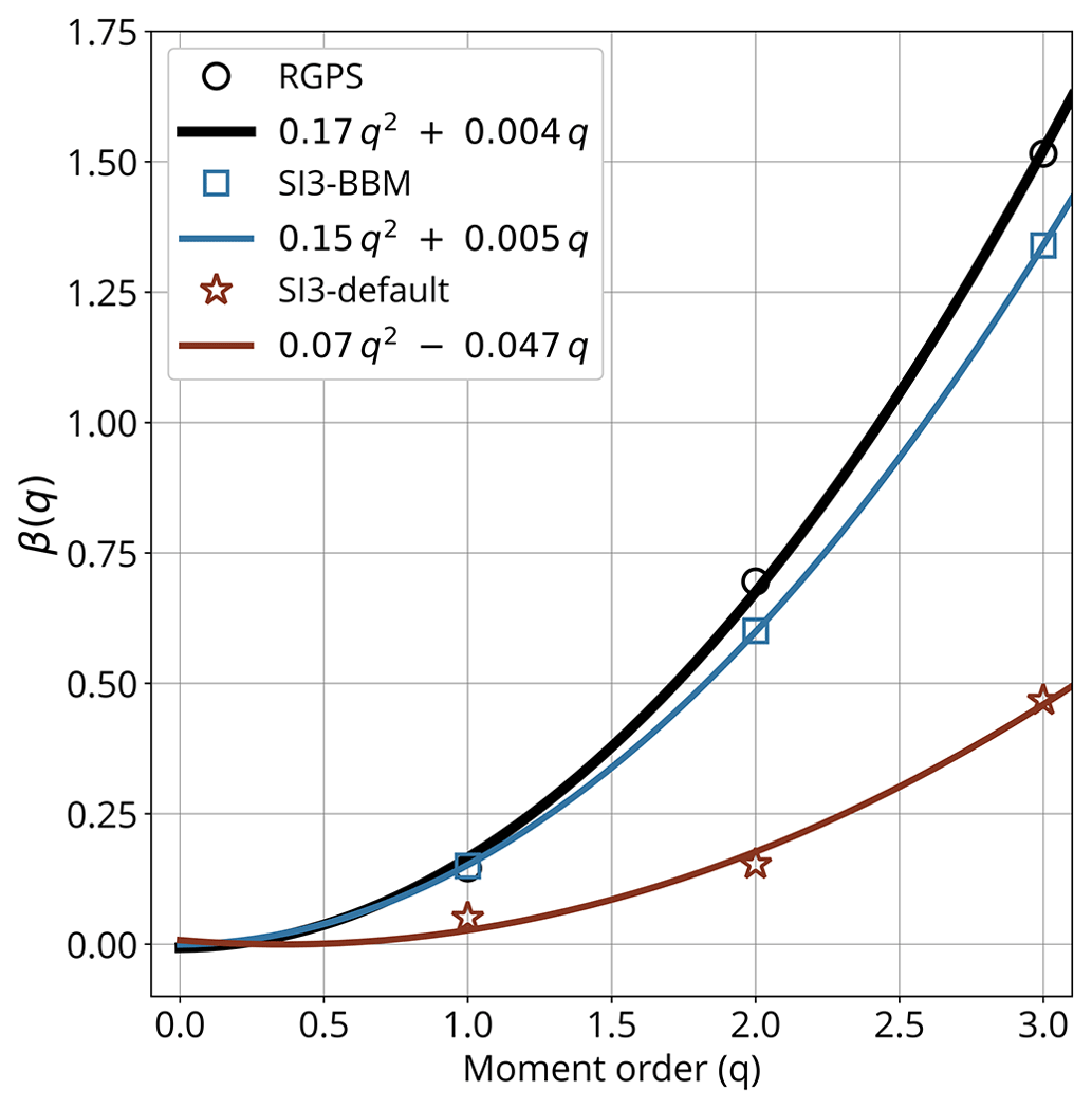
The simulated and observed structure functions (i.e., the dependence of the scaling exponents of the power law on the order of the moment) β(q) are shown in Fig. 11. The spatial scaling obtained from both the observations and SI3-BBM are multi-fractal because their structure functions is well approximated (in the sense of the least-square method) by a quadratic function of the type . One should note that in the universal multi-fractal formalism, the structure functions are not required to be quadratic and can have a varying degree of nonlinearity (Lovejoy and Schertzer, 2007). A quadratic structure function, as obtained here, simply means that the process of sea ice deformation can be approximated by a lognormal multiplicative cascade model with a maximum degree of multi-fractality. The structure function of SI3-BBM shows a curvature a that has a magnitude comparable to that of RGPS, i.e., 0.15 versus 0.17. These values of curvature are in fair agreement with those obtained from Lagrangian simulations performed with neXtSIM and reported in previous studies: 0.14 in Rampal et al. (2016) and 0.11 in Rampal et al. (2019).
4.1 On the numerical implementation
The cross-nudging has a noteworthy analogy to the Asselin filter (Asselin, 1972) used when discretizing time derivatives of a prognostic variable by means of the leap-frog scheme (three time levels, centered, and second-order), in particular in the context of shallow-water equations. The goal of this Asselin filter is to subtly average the solutions of neighboring time levels to prevent the separation of trajectories between the even and odd time step levels (Marsaleix et al., 2012). As such, the cross-nudging can be seen as a sort of spatial and two-dimensional analog to the Asselin filter. Despite the crudeness of this approach, which tends to be problematic due to the unavoidable loss of conservation properties, the Asselin filter is still largely used in modern CMIP-class OGCMs like NEMO. Indeed, the ocean component of NEMO used in the simulations presented in this study still relies on it. As of now, our cross-nudging approach clearly lacks physical and numerical consistency, but it somehow allows demonstrating that the implementation of a brittle rheology, along with the advection of the internal stress tensor, is feasible onto an E-augmented C-grid, provided a method to prevent the separation of solutions is used. Nevertheless, we plan to further investigate the possibility of implementing approaches that are more physically and numerically consistent. For instance, an option is to apply the cross-nudging to the two invariants of the stress tensor (i.e., σI and σII) and the rate of internal work of the ice. This would introduce three equations for three invariant quantities, from which the three components of the stress tensor could be deduced afterward. Another option is to explore the possibility of deriving a numerical formulation inspired from that of Mesinger (1973) and Janjić (1974), in which auxiliary velocity (or stress) points are introduced midway between the neighboring tracer (or velocity) points.
Another critical requirement, this time stemming from the use of the Eulerian and finite-difference framework, has to do with the ability of the advection scheme to advect fields with as little numerical diffusion or dispersion as possible. This is particularly critical when using a brittle rheology like BBM, as most fields exhibit sharp gradients, often associated with linear kinematic features. We chose to use the scheme of Prather (1986), the dispersive scheme option of SI3, to favor the conservation of sharp gradients at the cost of potential noise and overshoots reminiscent of the Gibbs phenomenon. One could, however, consider the use of a different approach that would optimize the advection of sharp gradients, for instance a spatial discretization based on the discontinuous Galerkin method. This method has proven to be efficient and accurate in treating the advection of sea ice variables in the case of a brittle sea ice rheology such as MEB (Dansereau et al., 2017) but has not yet been tested in the context of large-scale, long-term sea ice simulations. This is the scope of our present work and future papers.
Table 4Computational cost of 3 months (90 d) of pan-Arctic sea ice simulation at ° resolution with SI3 on the NANUK4 regional domain (31 vertical levels), with an advective time step of 720 s, run on 29 cores in parallel (with output data writing disabled to limit the influence of I/O). Default SI3 aEVP setup (NEVP=100) versus newly implemented BBM rheology (Ns=100) for both stand-alone (SI3-SAS) and coupled (SI3-OCE) modes.
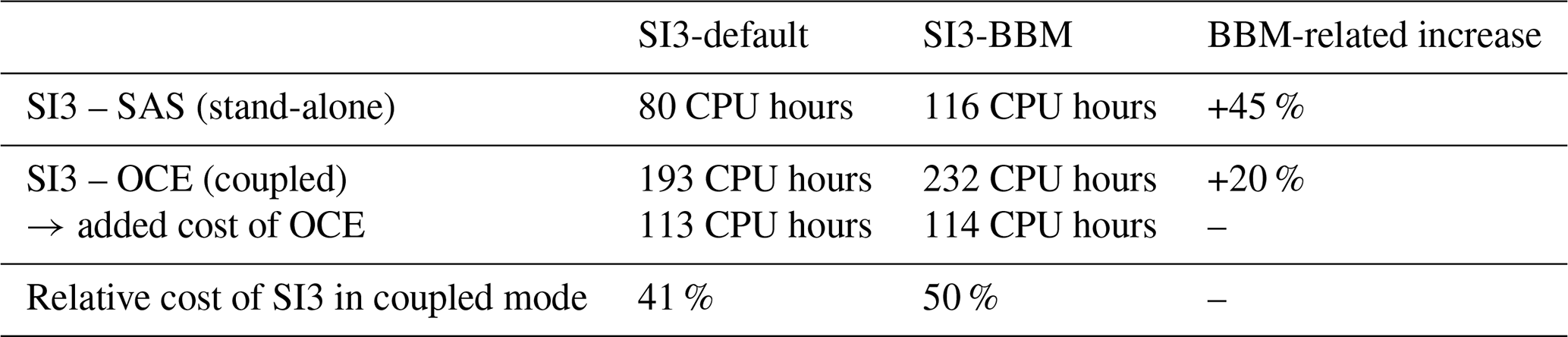
As discussed in Sect. 2.3.1, the use of the E-grid in the dynamics and advection modules of SI3 implies that equations specific to the momentum and the constitutive law are solved on both the T- and the F-centric grids. Moreover, with the need to advect the stress tensor and the damage tracer, specific to brittle rheologies, 2 × 4 additional scalar fields need to be advected. This inevitably leads to an increase in the computational cost of SI3. We have estimated this extra cost by comparing the wall-time length required to complete a 90 d simulation with each rheology using the same 29 cores in parallel on the same computer. Our results, summarized in Table 4, suggest that the increase in the computational cost associated with the use of BBM in place of aEVP is about 45 % when SI3 is used in a stand-alone mode (SAS). In standard coupled mode, with SI3 coupled to OCE, the BBM-related cost increase is about 20 %. This lower value is explained by the fact that by default, the coupling between OCE and SI3 is done sequentially. As such, the cost of SI3 simply adds up to that of OCE, and the cost of OCE is expected to be independent of the mode used (in our case: 113 and 114 CPU hours for SI3-default and SI3-BBM, respectively). Based on our results, the relative cost of SI3 in coupled mode is about 40 % when using the default aEVP setup and about 50 % with our BBM implementation.
4.2 On the simulated sea ice deformations
Based on comparisons against various types of observations, recent studies suggest that large-scale models using BBM can realistically simulate the dynamics and properties of sea ice (Ólason et al., 2022; Rheinlænder et al., 2022; Boutin et al., 2023; Regan et al., 2023). Yet, the deformation in convergence and the subgrid-scale processes related to sea ice ridging are not represented by BBM with the same degree of accuracy. The model overestimates the number of converging events with magnitudes of about 1 % to 5 % per day and underestimates the most extreme events (Fig. 8c and Ólason et al., 2022). As of now, parameter tuning, in particular that of the BBM-specific ridging threshold parameter Pmax, has not helped to improve the agreement with the observed PDFs of convergence (not shown). Therefore, we conclude that some fundamental processes need to be reconsidered in BBM.
In Sect. 3.3.3, we find that the degree of multi-fractality of the deformation fields simulated by SI3-BBM is slightly lower than that obtained from the RGPS data. The fact that the deformation fields simulated by neXtSIM in Ólason et al. (2022) are in better agreement with RGPS in this regard suggests that this problem is linked to some numerical aspects of our BBM implementation rather than the BBM rheology itself. This is most likely the consequence of the introduction of some additional numerical dispersion and diffusion by the advection scheme and the cross-nudging treatment, respectively, as these two features are absent in neXtSIM. Moments of order 2 and 3 are expected to be more affected than the mean by an unwanted source of noise and diffusion, which might explain why SI3-BBM reproduces the mean across all scales remarkably well and why the power-law exponents for the variance and the skewness are underestimated. In this regard, the use of the finite-element method together with the discontinuous Galerkin method might prove to be a promising combination to simulate the multi-fractality of sea ice deformation even more accurately while remaining in the Eulerian and quadrilateral mesh framework.
The brittle Bingham–Maxwell rheology, known as BBM, has been successfully implemented into SI3, the CMIP-class, Eulerian finite-difference sea ice model of the NEMO modeling system. We have shown that our implementation, which features a prognostic ice damage tracer and a prognostic internal stress tensor, is able to realistically simulate sea ice deformation statistics on a pan-Arctic scale when compared to satellite observations.
Our implementation uses a new discretization approach that expands the C-grid of NEMO into the Arakawa E-grid in the parts of the code dedicated to sea ice dynamics. We have chosen to do so in order to (i) avoid resorting to the spatial averaging of prognostic fields, in particular the damage tracer, as an interpolation technique between the center and corner points of the grid cells, and (ii) allow the straightforward advection of the shear component of the stress tensor. However, by solving the dynamics on the E-grid, the issue of the grid separation is introduced. We have introduced a simple technique to prevent this grid separation in the form of the cross-nudging. This cross-nudging relies on the averaging of the components of the stress tensor and, as such, introduces a spatial smoothing of these components. Despite the fact that this aspect of our implementation is in contradiction to one of our initial motivations (i.e., avoid the use of spatial averaging), we think that our E-augmented C-grid approach is promising. This is because the damage tracer is never averaged, which we think is beneficial for the consistency of the brittle model, and the advection of the shear component of the stress tensor is straightforward and numerically consistent with that of the trace components.
For the advection of the stress tensor, we have chosen to use the upper-convected time derivative rather than its lower-convected counterpart, a combination of the two, or simply the standard material derivative. This choice, based on arbitrary considerations, has no significant impact on the deformation statistics presented in this paper. Both formulations are available in our implementation, which will allow SI3 users to further investigate on this matter, in particular by means of dedicated idealized test cases.
We carried out a statistical analysis of the sea ice deformation rates obtained from a set of realistic pan-Arctic coupled ocean–sea ice simulations for winter 1996–1997, performed with SI3 at a horizontal resolution of about 12 km. Based on a comparison with satellite observations, this analysis demonstrates that the use of the newly implemented BBM rheology results in simulated sea ice deformation statistics that are realistic. In particular, we show that the use of BBM allows simulating highly localized (nearly linear) kinematic features within the sea ice cover, along which the most substantial deformation rates are concentrated.
The observed non-Gaussian statistics of the sea ice deformation process are clearly present in the simulation that uses our newly implemented BBM rheology, except the most extreme values and more particularly those corresponding to the convergent mode of deformation. Since this drawback was already observed in the BBM-driven simulations of the Lagrangian sea ice model neXtSIM presented in Ólason et al. (2022), we think that it probably shows an intrinsic limitation of the current BBM rheological model, an issue that certainly merits investigating and fixing in the future. Finally, we show that the observed spatial scaling invariance property of sea ice deformation, and in particular its multi-fractal nature, is fairly well captured by the BBM-driven simulation but with a slightly lower degree of multi-fractality.
A1 Table of symbols used in the text
| Symbol | Definition | Units |
| m | mass of ice and snow per unitarea | kg m−2 |
| ρi | density of sea ice | kg m−3 |
| ρw | density of seawater | kg m−3 |
| sea ice velocity | m s−1 | |
| A | sea ice fraction | – |
| h | sea ice thickness | m |
| g | acceleration of gravity | m s−2 |
| f | Coriolis frequency | s−1 |
| k | vertical unit vector (z axis) | s−1 |
| H | sea surface height | m |
| τ | ice–ocean stress | Pa |
| τa | wind (ice–atmosphere) stress | Pa |
| σ | internal stress tensor (2 × 2) | Pa |
| strain rate tensor (2 × 2) | s−1 | |
| d | damage of sea ice | – |
| Δx | local resolution (size) of the gridmesh | m |
| C | compaction parameter | – |
| α | damage parameter (Dansereau, 2016) | – |
| E0,E | elastic modulus of undamaged and damaged ice | Pa |
| λ0,λ | apparent viscous relaxation time of undamagedand damaged ice | s |
| BBM-specific ridging term | – | |
| Pmax | ridging threshold | Pa |
| P0 | scaling parameter for Pmax | Pa |
| h0 | reference ice thickness for Pmax | m |
| c | sea ice cohesion | Pa |
| ν | Poisson's ratio | – |
| σI | isotropic normal stress (firstinvariant of stress tensor) | Pa |
| σII | maximum shear stress (secondinvariant of stress tensor) | Pa |
| μ | internal friction coefficient | – |
| N | upper limit for compressivestress | Pa |
| CE | propagation speed of an elasticshear wave | m s−1 |
| td | characteristic timescale for thepropagation of damage | s |
| dcrit | damage increment (Dansereau, 2016) | – |
| kth | healing constant for damage | K s |
| ΔTh | temperature difference betweenbottom and surface of ice | K |
A2 Acronyms
| NEMO | Nucleus for European Modeling of the Ocean |
| SI3 | Sea-Ice modeling Integrated Initiative (sea icecomponent of NEMO) |
| OCE | 3D ocean component of NEMO |
| SAS | Stand-alone surface module of NEMO (i.e.,SI3 stand-alone) |
| LIM | Louvain-La-Neuve sea-Ice Model |
| BBM | Brittle Bingham–Maxwell (rheology) |
| MEB | Maxwell elasto-brittle (rheology) |
| VP | Viscous–plastic (rheology) |
| FD | Finite difference (method) |
| CN | Cross-nudging (treatment) |
| Probability density function | |
| LKFs | Linear kinematic features |
| GCM | General circulation model |
| OGCM | Ocean general circulation model |
| SST | Sea surface temperature |
| SSH | Sea surface height |
| RGPS | RADARSAT Geophysical Processor System(dataset) |
A3 Notations related to the discretization on the E-grid
The bar + superscript notation refers to a spatial interpolation; is field ϕ interpolated onto X points.
Interpolation from T- to F-points, or conversely, is based on the average of the four nearest surrounding points (Fig. 3a).
Note: surrounding points located on land or open-boundary cells are excluded from the averaging.
For the interpolation from tracer (T or F) to velocity (U or V) points, or conversely, only the two nearest surrounding points are used.
The “hat” notation refers to the F-centric counterpart of x, with x being a prognostic scalar or tensor (rank 1 or 2) defined in the T-centric grid (mind that if x is the element of a tensor, is not necessarily defined on F-points). Example: and are prognostic fields defined on F-points (the natural location for d and σ11 on the C-grid is the T-point); similarly, is defined on T-points (the natural location for σ12 on the C-grid is the F-point).
A4 Miscellaneous notations
| symmetric tensor x expressed in its Voigt form | |
| x(i) | initial estimate of variable x |
| at X | on the X points of the grid |
| σkl | vertically integrated components of tensor σ |
| if σkl defined at T | |
| if σkl defined at F | |
| upper-convected time derivative of symmetric(rank 2) tensor x | |
| lower-convected time derivative of symmetric(rank 2) tensor x |
A5 Table of symbols related to the numerical implementation
| Symbol | Definition | Units |
| ΔT | advective time step for the advection and the thermodynamics | s |
| Δt | dynamical time stepspecific to BBM (time splitting) |
s |
| Ns | , time-splittingparameter | – |
| k | time level index of timesplitting () | – |
| ice concentration, thickness, and damage of iceat T | –, m, – | |
| ice concentrationand thickness interpolated at F | –, m | |
| damage of ice at F | – | |
| strain rate tensor (2 × 2)of the T-centric cell | s−1 | |
| strain rate tensor (2 × 2)of the F-centric cell | s−1 | |
| internal stress tensor(2×2) of the T-centric cell | Pa | |
| internal stress tensor(2×2) of the F-centric cell | Pa | |
| ice concentration interpolated at U and at V | m |
| ice thickness interpolatedat U and at V | m | |
| u,v | ice velocity at the Δt level(at U and at V) | m s−1 |
| ice velocity at the Δt level(at V and at U) | m s−1 | |
| U,V | ice velocity at the ΔTlevel (at U and at V) | m s−1 |
| ice velocity at the ΔTlevel (at V and at U) | m s−1 | |
| ice–ocean drag coefficient | – | |
| τx,τy | ice–ocean stress at U andat V | Pa |
| ice–ocean stress at V andat U | Pa | |
| uo,vo | surface ocean current at Uand at V | m s−1 |
| γcn | cross-nudging coefficient | – |
| ice–atmosphere drag coefficient | – | |
| Δ𝚃x | T-centered Δx that connects two neighboringU-points | m |
| Δ𝚃y | T-centered Δy that connects two neighboringV-points | m |
| Δ𝙵x | F-centered Δx that connects two neighboringV-points | m |
| Δ𝙵y | F-centered Δy that connects two neighboringU-points | m |
| Δ𝚄x | U-centered Δx that connects two neighboringT-points | m |
| Δ𝚄y | U-centered Δy that connects two neighboringF-points | m |
| Δ𝚅x | V-centered Δx that connects two neighboringF-points | m |
| Δ𝚅y | V-centered Δy that connects two neighboringT-points | m |
B1 Algorithm
Time-splitting loop (Δt)/for k=1 to Ns
-
Compute elasticity and viscous relaxation time as a function of damage and current sea ice concentration (Eqs. B5 and B6).
-
Compute the normal stress invariant of σk and → (Eq. B8).
-
Compute as a function of current sea ice thickness and concentration (Eq. B7).
-
Compute as a function of and (Eq. B9).
-
Compute the three components of each strain rate tensor based on sea ice velocities at time level k (Eqs. B1, B2, B3, and B4).
-
Calculate an initial prognostic estimate of the stress tensors at time level and (Eq. B11).
-
Apply cross-nudging between the vertically integrated σ(i)k+1 and (Eq. 16).
-
Apply a Mohr–Coulomb test on σ(i)k+1 and .
-
Calculate a prognostic estimate of the stress tensors and damage at time level , dk+1 and , .
-
Compute the divergence of the vertically integrated σk+1 and (Eqs. B16 and B17).
-
Calculate a prognostic estimate of sea ice velocity at time level and (Eqs. B19 and B18).
SI3 (advective) time step (ΔT):
-
BBM rheology (time-splitting loop above)
-
Advection of generic SI3 prognostic tracers (A, h, etc.) at T-points using U and V
-
Advection of d, σ11, σ22, and at T-points using U and V
-
Advection of , , , and σ12 at F-points using and
-
Healing of damage (d and ) (Eq.14)
-
Thermodynamics module of SI3 (update of A, h, etc.)
B2 Update of internal stress tensor in the T- and F-centric worlds
B2.1 Divergence, shear, and strain rate tensor of ice velocity
Following Hunke and Dukowicz (2002), here is how the components of the strain rate of the sea ice velocity vector are computed on the T- and F-centric grids based on the finite-difference method.
-
Divergence rate :
-
Tension rate :
-
Shear rate :
From the above, the three components of the 2D strain rate tensors are obtained.
B2.2 Update of the stress tensors
-
Elasticity and viscous relaxation time of damaged ice
Note that it is the averaged value of A at F-points, , that is used in the equations for the F-centric grid.
-
Ridging threshold
Note that it is the averaged value of h at F-points, , that is used in the second equation.
-
Invariants of stress tensor
-
term
-
Multiplicator for stress update
-
Initial update of stress tensor
-
Damage increment
-
Update of damage and stress tensors
-
In regions where , the following applies.
-
Elsewhere, the following applies.
-
B3 Momentum equation
As opposed to aEVP for which SI3 uses the scheme of Kimmritz et al. (2016, 2017), here we chose to solve the equation for momentum (in both the T- and F-centric worlds) using the implicit scheme approach of Bouillon et al. (2009).
B3.1 Divergence of the vertically integrated stress tensor
-
Definition
-
Discretized in the T-centric cell
-
Discretized in the F-centric cell
B3.2 Update of sea ice velocity
For clarity, we gather the contributions of the wind stress, the Coriolis term, and the SSH tilt vectors in a single vector term named (Rx,Ry). This is because these three terms do not present any particular challenge to express with respect to the existing implementation of aEVP. Note, however, that with the E-grid no spatial interpolation is needed to express the discretized Coriolis term.
Implicitness of the scheme is introduced through the use of sea ice velocity at level k+1 in the estimate of the basal ice–water stress vector (τx,τy).
Then, the discretized equation of momentum yields the expression of the two velocity components at time level k+1.
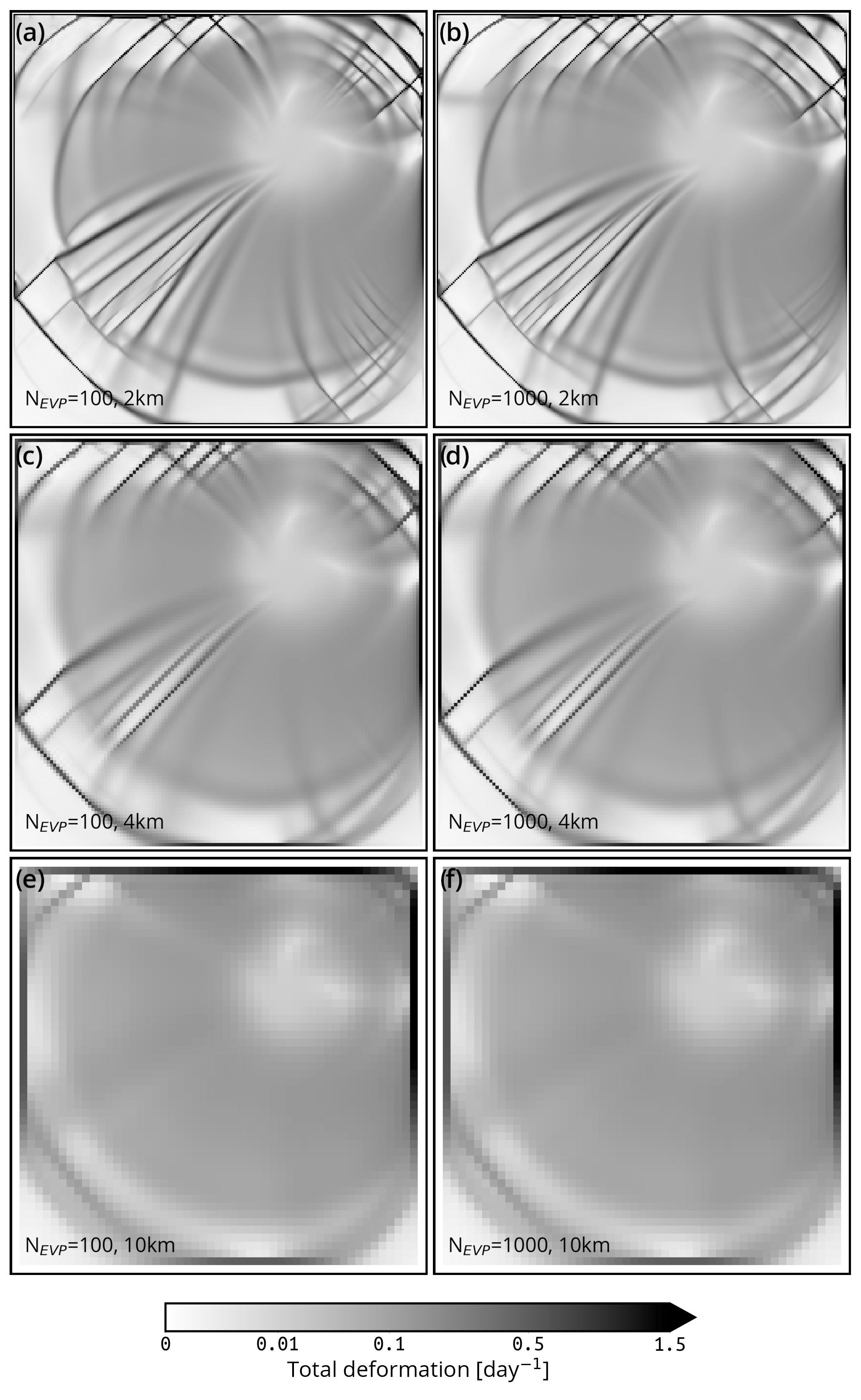
Figure C1Sea ice total deformation (instantaneous) in the test case described by Mehlmann et al. (2021) after 48 h of simulation with SI3 using the default SI3 aEVP rheology with NEVP=100 and NEVP=1000 (left-hand and right-hand column, respectively) at 2, 4, and 10 km resolution (first, second, and third row, respectively).
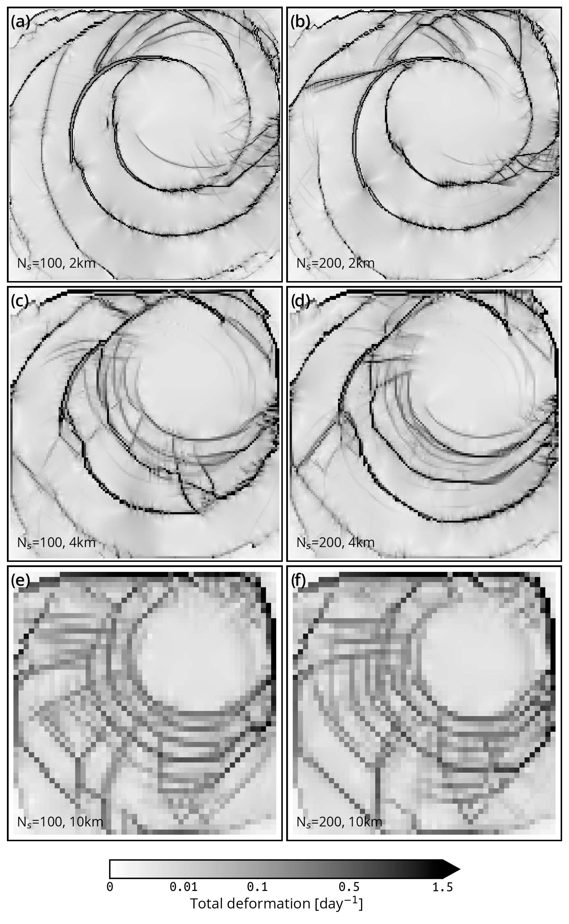
Figure C2Sea ice total deformation (instantaneous) in the test case described by Mehlmann et al. (2021) after 48 h of simulation with SI3 using the newly implemented BBM rheology with Ns=100 and Ns=200 (left-hand and right-hand column, respectively) at 2, 4, and 10 km resolution (first, second, and third row, respectively).
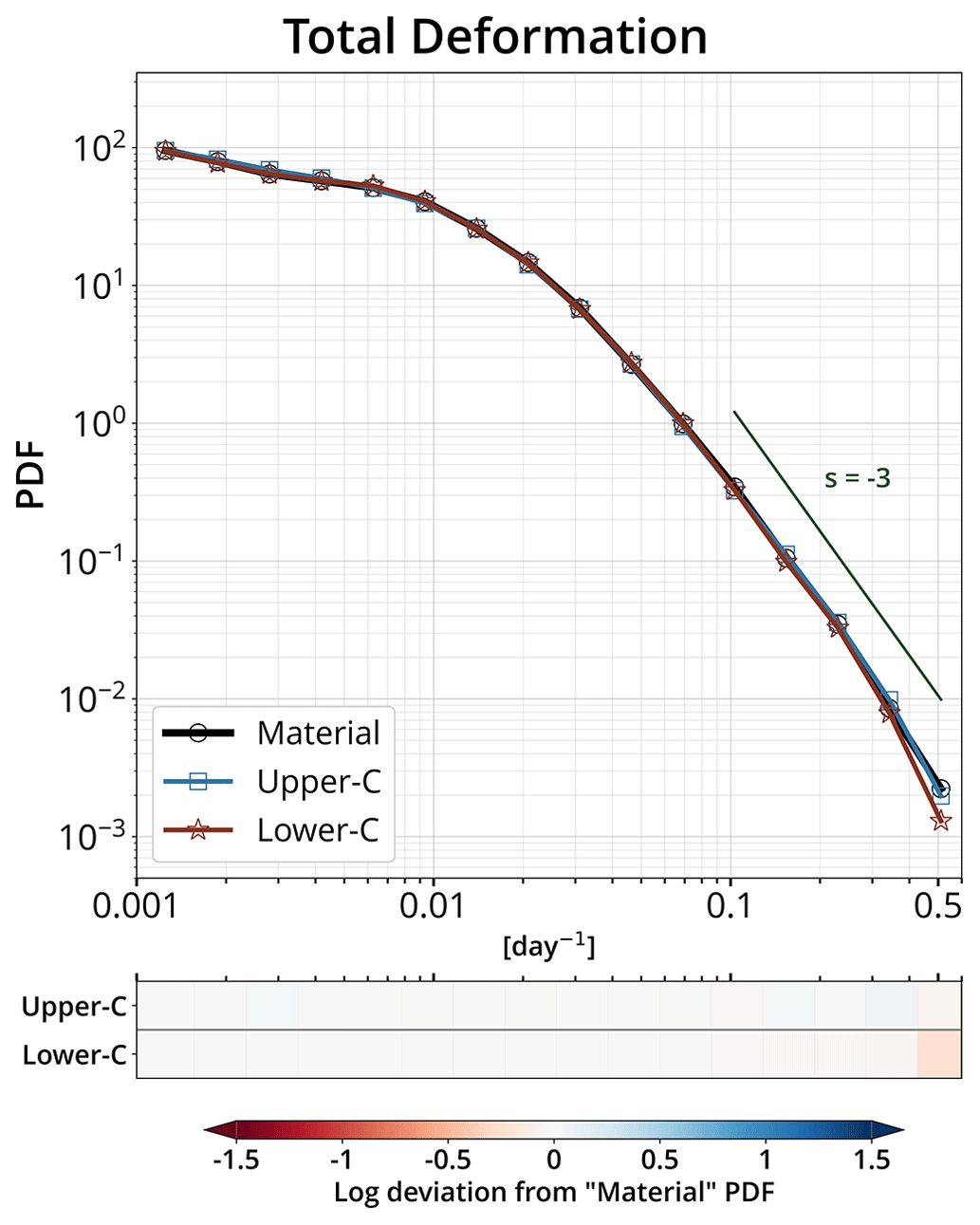
Figure C3PDFs of the total deformation rates at the 10 km spatial and 3 d temporal scale for the synthetic counterparts of RGPS data constructed using the simulated sea ice velocities of three BBM-driven SI3 experiments that use different time-derivative formulations for the stress tensor: only material derivative (“Material”, black line with circle markers), upper-convected time derivative as in SI3-BBM (“Upper-C”, blue line with square markers), and lower-convected time derivative (“Lower-C”, red line with star markers).
-
The NEMO source code used to perform the experiments is based on the official release 4.2.2 of NEMO; it is available on Zenodo with the DOI https://doi.org/10.5281/zenodo.11551599 (The NEMO team, 2024).
-
New and modified Fortran-90 source files relative to our implementation of the BBM rheology in version 4.2.2 of NEMO/SI3 are available on Zenodo with the DOI https://doi.org/10.5281/zenodo.11581840 (Brodeau, 2024a).
-
The Python software used to seed and build Lagrangian trajectories out of the SI3 hourly sea ice velocities is named
sitrack; the version used to perform the present study is available on Zenodo with the DOI https://doi.org/10.5281/zenodo.10457918 (Brodeau, 2024b). -
The Python software used to compute the RGPS and model-based sea ice deformation rates based on quadrangles and perform the scaling analysis is named
mojito; the version used to perform the present study is available on Zenodo with the DOI https://doi.org/10.5281/zenodo.10457924 (Brodeau, 2924c). -
Model data produced and analyzed in this study, namely SI3 hourly output files for pan-Arctic simulations SI3-BBM and SI3-default, are available on Zenodo with the DOI https://doi.org/10.5281/zenodo.11582103 (Brodeau, 2024d).
-
Model data as well as setup, forcing, and configuration files for the “cyclone” test case experiments (Mehlmann et al., 2021) discussed and analyzed in this study are available on Zenodo with the DOI https://doi.org/10.5281/zenodo.11615982 (Brodeau, 2024e).
This study is based on the original idea of PR and EÓ, who suggested using the E-grid. The implementation of the BBM rheology into SI3 has been carried out by LB, with the help of PR. The numerical simulations and statistical analyses have been performed by LB. LB also prepared all the figures. Interpretations of the results were provided by LB, PR, and EÓ. LB and PR led the writing of the manuscript, incorporating input from EÓ. Suggestions and improvements on the text have also been provided by VD.
The contact author has declared that none of the authors has any competing interests.
Publisher's note: Copernicus Publications remains neutral with regard to jurisdictional claims made in the text, published maps, institutional affiliations, or any other geographical representation in this paper. While Copernicus Publications makes every effort to include appropriate place names, the final responsibility lies with the authors.
We would like to express our gratitude to one anonymous reviewer and Mathieu Plante for conducting a thorough and constructive review. Their comments and suggestions have greatly contributed to improving and clarifying this manuscript.
This research received support through Schmidt Sciences, LLC, via the SASIP project (grant G-24-66154).
This paper was edited by Riccardo Farneti and reviewed by Mathieu Plante and two anonymous referees.
Arakawa, A.: Design of the UCLA general circulation model, Tech. Rept. No. 7, 116 pp., University of California at Los Angeles, CA, 90024, 1972. a
Arakawa, A. and Lamb, V. R.: Computational Design of the Basic Dynamical Processes of the UCLA General Circulation Model, in: Methods in Computational Physics: Advances in Research and Applications, edited by: Chang, J., Elsevier, https://doi.org/10.1016/b978-0-12-460817-7.50009-4, ISBN 9780124608177; ISSN: 0076-6860, pp. 173–265, 1977. a, b, c
Asselin, R.: Frequency Filter for Time Integrations, Mon. Weather Rev., 100, 487–490, https://doi.org/10.1175/1520-0493(1972)100<0487:fffti>2.3.co;2, 1972. a
Barnier, B., Madec, G., Penduff, T., Molines, J.-M., Treguier, A.-M., Sommer, J. L., Beckmann, A., Biastoch, A., Böning, C., Dengg, J., Derval, C., Durand, E., Gulev, S., Remy, E., Talandier, C., Theetten, S., Maltrud, M., McClean, J., and Cuevas, B. D.: Impact of partial steps and momentum advection schemes in a global ocean circulation model at eddy-permitting resolution, Ocean Dynam., 56, 543–567, 2006. a
Bouchat, A. and Tremblay, B.: Using sea-ice deformation fields to constrain the mechanical strength parameters of geophysical sea ice, J. Geophys. Res.-Oceans, 122, 5802–5825, https://doi.org/10.1002/2017jc013020, 2017. a
Bouchat, A., Hutter, N., Chanut, J., Dupont, F., Dukhovskoy, D., Garric, G., Lee, Y., Lemieux, J.-F., Lique, C., Losch, M., Maslowski, W., Myers, P. G., Ólason, E., Rampal, P., Rasmussen, T., Talandier, C., Tremblay, B., and Wang, Q.: Sea Ice Rheology Experiment (SIREx), part I: Scaling and statistical properties of sea-ice deformation fields, J. Geophys. Res.-Oceans, 127, e2021JC017667, https://doi.org/10.1029/2021jc017667, 2022. a, b, c, d
Bouillon, S. and Rampal, P.: Presentation of the dynamical core of neXtSIM, a new sea ice model, Ocean Model., 91, 23–37, https://doi.org/10.1016/j.ocemod.2015.04.005, 2015. a
Bouillon, S., Maqueda, M. Á. M., Legat, V., and Fichefet, T.: An elastic–viscous–plastic sea ice model formulated on Arakawa B and C grids, Ocean Model., 27, 174–184, https://doi.org/10.1016/j.ocemod.2009.01.004, 2009. a
Boutin, G., Ólason, E., Rampal, P., Regan, H., Lique, C., Talandier, C., Brodeau, L., and Ricker, R.: Arctic sea ice mass balance in a new coupled ice–ocean model using a brittle rheology framework, The Cryosphere, 17, 617–638, https://doi.org/10.5194/tc-17-617-2023, 2023. a, b
Brodeau, L.: brodeau/bbm4si3: 1.1.0 (1.1.0), Zenodo [code], https://doi.org/10.5281/zenodo.11581840, 2024a. a
Brodeau, L.: brodeau/sitrack: 1.0 (1.0), Zenodo [code], https://doi.org/10.5281/zenodo.10457918, 2024b. a
Brodeau, L.: brodeau/mojito: 1.0 (1.0), Zenodo [code], https://doi.org/10.5281/zenodo.10457924, 2024. a
Brodeau, L.: SI3 sea-ice hourly output for SI3-BBM and SI3-default Pan-Arctic simulations (Brodeau et al., 2024, final version), Zenodo [data set], https://doi.org/10.5281/zenodo.11582103, 2024d. a
Brodeau, L.: NEMO/SAS-SI3 setup, forcing and output for SI3-BBM and SI3-default idealized “cyclone” simulations (Brodeau et al., 2024, final version), Zenodo [data set], https://doi.org/10.5281/zenodo.11615982, 2024e. a
Coon, M. D., Maykut, S. A., Pritchard, R. S., Rothrock, D. A., and Thorndike, A. S.: Modeling the pack ice as an elastic-plastic material, AIDJEX Bull., 24, 1–105, 1974. a
Danilov, S., Mehlmann, C., and Fofonova, V.: On discretizing sea-ice dynamics on triangular meshes using vertex, cell or edge velocities, Ocean Model., 170, 101937, https://doi.org/10.1016/j.ocemod.2021.101937, 2022. a
Danilov, S., Mehlmann, C., Sidorenko, D., and Wang, Q.: CD-type discretization for sea ice dynamics in FESOM version 2, Geosci. Model Dev., 17, 2287–2297, https://doi.org/10.5194/gmd-17-2287-2024, 2024. a
Dansereau, V.: A Maxwell-Elasto-Brittle model for the drift and deformation of sea ice, PhD thesis, Université Grenoble Alpes, Grenoble, France, 2016. a, b
Dansereau, V., Weiss, J., Saramito, P., and Lattes, P.: A Maxwell elasto-brittle rheology for sea ice modelling, The Cryosphere, 10, 1339–1359, https://doi.org/10.5194/tc-10-1339-2016, 2016. a, b, c, d, e, f, g
Dansereau, V., Weiss, J., Saramito, P., Lattes, P., and Coche, E.: Ice bridges and ridges in the Maxwell-EB sea ice rheology, The Cryosphere, 11, 2033–2058, https://doi.org/10.5194/tc-11-2033-2017, 2017. a
Ferry, N., Barnier, B., Garric, G., Haines, K., Masina, S., Parent, L., Storto, A., Valdivieso, M., Guinehut, S., and Mulet, S.: NEMO: the modelling engine of global ocean reanalyses, Mercator Ocean Quarterly Newsletter, 46, 46–59, 2012. a
Hersbach, H., Bell, B., Berrisford, P., Hirahara, S., Horányi, A., Muñoz-Sabater, J., Nicolas, J., Peubey, C., Radu, R., Schepers, D., Simmons, A., Soci, C., Abdalla, S., Abellan, X., Balsamo, G., Bechtold, P., Biavati, G., Bidlot, J., Bonavita, M., Chiara, G., Dahlgren, P., Dee, D., Diamantakis, M., Dragani, R., Flemming, J., Forbes, R., Fuentes, M., Geer, A., Haimberger, L., Healy, S., Hogan, R. J., Hólm, E., Janisková, M., Keeley, S., Laloyaux, P., Lopez, P., Lupu, C., Radnoti, G., Rosnay, P., Rozum, I., Vamborg, F., Villaume, S., and Thépaut, J.-N.: The ERA5 global reanalysis, Q. J. Roy. Meteor. Soc., 146, 1999–2049, https://doi.org/10.1002/qj.3803, 2020. a
Hibler, W. D.: A dynamic thermodynamic sea ice model, J. Phys. Oceanogr., 9, 815–846, https://doi.org/10.1175/1520-0485(1979)009<0815:adtsim>2.0.co;2, 1979. a
Hinch, J. and Harlen, O.: Oldroyd B, and not A?, J. Non-Newton. Fluid, 298, 104668, https://doi.org/10.1016/j.jnnfm.2021.104668, 2021. a, b
Hopkins, M. A.: Four stages of pressure ridging, J. Geophys. Res.-Oceans, 103, 21883–21891, https://doi.org/10.1029/98jc01257, 1998. a
Hunke, E. C. and Dukowicz, J. K.: The Elastic–Viscous–Plastic Sea Ice Dynamics Model in General Orthogonal Curvilinear Coordinates on a Sphere—Incorporation of Metric Terms, Mon. Weather Rev., 130, 1848–1865, https://doi.org/10.1175/1520-0493(2002)130<1848:tevpsi>2.0.co;2, 2002. a
Hutter, N., Losch, M., and Menemenlis, D.: Scaling Properties of Arctic Sea Ice Deformation in a High-Resolution Viscous-Plastic Sea Ice Model and in Satellite Observations, J. Geophys. Res.-Oceans, 123, 672–687, https://doi.org/10.1002/2017jc013119, 2018. a, b
Hutter, N., Bouchat, A., Dupont, F., Dukhovskoy, D., Koldunov, N., Lee, Y. J., Lemieux, J.-F., Lique, C., Losch, M., Maslowski, W., Myers, P. G., Ólason, E., Rampal, P., Rasmussen, T., Talandier, C., Tremblay, B., and Wang, Q.: Sea Ice Rheology Experiment (SIREx): 2. Evaluating Linear Kinematic Features in High-Resolution Sea Ice Simulations, J. Geophys. Res.-Oceans, 127, e2021JC017666, https://doi.org/10.1029/2021jc017666, 2022. a, b
IPCC: The Ocean and Cryosphere in a Changing Climate: Special Report of the Intergovernmental Panel on Climate Change, Cambridge University Press, Cambridge, UK, https://doi.org/10.1017/9781009157964.005, pp. 203–320, 2022. a
Janjić, Z. I.: A Stable Centered Difference Scheme Free of Two-Grid-Interval Noise, Mon. Weather Rev., 102, 319–323, https://doi.org/10.1175/1520-0493(1974)102<0319:ASCDSF>2.0.CO;2, 1974. a, b, c
Janjić, Z. I.: Nonlinear Advection Schemes and Energy Cascade on Semi-Staggered Grids, Mon. Weather Rev., 112, 1234–1245, https://doi.org/10.1175/1520-0493(1984)112<1234:nasaec>2.0.co;2, 1984. a
Janjić, Z. I. and Mesinger, F.: Finite difference methods for the shallow water equations on various horizontal grids, in: Numerical Methods for Weather Prediction, vol. 1, Seminar 1983, ECMWF, Shinfield Park, Reading, p. 29–101, 1984. a
Kagan, Y. Y. and Jackson, D. D.: Long-Term Earthquake Clustering, Geophys. J. Int., 104, 117–134, https://doi.org/10.1111/j.1365-246x.1991.tb02498.x, 1991. a
Kimmritz, M., Danilov, S., and Losch, M.: The adaptive EVP method for solving the sea ice momentum equation, Ocean Model., 101, 59–67, https://doi.org/10.1016/j.ocemod.2016.03.004, 2016. a, b, c, d
Kimmritz, M., Losch, M., and Danilov, S.: A comparison of viscous-plastic sea ice solvers with and without replacement pressure, Ocean Model., 115, 59–69, https://doi.org/10.1016/j.ocemod.2017.05.006, 2017. a
Konor, C. S. and Randall, D. A.: Impacts of the horizontal and vertical grids on the numerical solutions of the dynamical equations – Part 1: Nonhydrostatic inertia–gravity modes, Geosci. Model Dev., 11, 1753–1784, https://doi.org/10.5194/gmd-11-1753-2018, 2018. a
Kwok, R.: Deformation of the Arctic Ocean Sea Ice Cover between November 1996 and April 1997: A Qualitative Survey, in: IUTAM Symposium on Scaling Laws in Ice Mechanics and Ice Dynamics, edited by: Dempsey, J. P. and Shen, H. H., Springer Netherlands, Dordrecht, 315–322, ISBN 978-94-015-9735-7, https://doi.org/10.1007/978-94-015-9735-7_26, p. 315–322, 2001. a
Kwok, R., Schweiger, A., Rothrock, D. A., Pang, S., and Kottmeier, C.: Sea ice motion from satellite passive microwave imagery assessed with ERS SAR and buoy motions, J. Geophys. Res.-Oceans, 103, 8191–8214, https://doi.org/10.1029/97jc03334, 1998. a, b
Larson, R. G.: Constitutive Equations for Polymer Melts and Solutions, Elsevier, https://doi.org/10.1016/c2013-0-04284-3, ISBN 978-0-409-90119-1, 1988. a
Lemieux, J., Tremblay, B., Thomas, S., Sedláček, J., and Mysak, L. A.: Using the preconditioned Generalized Minimum RESidual (GMRES) method to solve the sea-ice momentum equation, J. Geophys. Res.-Oceans (1978–2012), 113, C10004, https://doi.org/10.1029/2007jc004680, 2008. a
Lemieux, J.-F., Knoll, D. A., Losch, M., and Girard, C.: A second-order accurate in time IMplicit–EXplicit (IMEX) integration scheme for sea ice dynamics, J. Comput. Phys., 263, 375–392, https://doi.org/10.1016/j.jcp.2014.01.010, 2014. a
Lindsay, R. W. and Stern, H. L.: The RADARSAT Geophysical Processor System: Quality of Sea Ice Trajectory and Deformation Estimates, J. Atmos. Ocean. Tech., 20, 1333–1347, https://doi.org/10.1175/1520-0426(2003)020<1333:trgpsq>2.0.co;2, 2003. a
Losch, M., Menemenlis, D., Campin, J.-M., Heimbach, P., and Hill, C.: On the formulation of sea-ice models. Part 1: Effects of different solver implementations and parameterizations, Ocean Model., 33, 129–144, https://doi.org/10.1016/j.ocemod.2009.12.008, 2010. a, b
Lovejoy, S. and Schertzer, D.: Nonlinear Dynamics in Geosciences, vol. 59 of Nonlinear Dynamics in Geosciences, Springer New York, New York, NY, https://doi.org/10.1007/978-0-387-34918-3_18, pp. 311–337,2007. a
Madec, G., Bourdallé-Badie, R., Chanut, J., Clementi, E., Coward, A., Ethé, C., Iovino, D., Lea, D., Lévy, C., Lovato, T., Martin, N., Masson, S., Mocavero, S., Rousset, C., Storkey, D., Müeller, S., Nurser, G., Bell, M., Samson, G., Mathiot, P., Mele, F., and Moulin, A.: NEMO ocean engine, Zenodo, https://doi.org/10.5281/zenodo.1464816, 2022. a
Maier-Reimer, E., Mikolajewicz, U., and Hasselmann, K.: Mean Circulation of the Hamburg LSG OGCM and Its Sensitivity to the Thermohaline Surface Forcing, J. Phys. Oceanogr., 23, 731–757, https://doi.org/10.1175/1520-0485(1993)023<0731:mcothl>2.0.co;2, 1993. a, b
Marsaleix, P., Auclair, F., Duhaut, T., Estournel, C., Nguyen, C., and Ulses, C.: Alternatives to the Robert–Asselin filter, Ocean Model., 41, 53–66, https://doi.org/10.1016/j.ocemod.2011.11.002, 2012. a
Marsan, D. and Weiss, J.: Space/time coupling in brittle deformation at geophysical scales, Earth Planet. Sc. Lett., 296, 353–359, https://doi.org/10.1016/j.epsl.2010.05.019, 2010. a
Marsan, D., Stern, H., Lindsay, R., and Weiss, J.: Scale dependence and localization of the deformation of arctic sea ice, Phys. Rev. Lett., 93, 178501, https://doi.org/10.1103/physrevlett.93.178501, 2004. a
Mehlmann, C., Danilov, S., Losch, M., Lemieux, J. F., Hutter, N., Richter, T., Blain, P., Hunke, E. C., and Korn, P.: Simulating Linear Kinematic Features in Viscous-Plastic Sea Ice Models on Quadrilateral and Triangular Grids With Different Variable Staggering, J. Adv. Model. Earth Sy., 13, e2021MS002523, https://doi.org/10.1029/2021ms002523, 2021. a, b, c, d, e, f, g, h
Mesinger, F.: A method for construction of second-order accuracy difference schemes permitting no false two-grid-interval wave in the height field, Tellus, 25, 444–458, https://doi.org/10.1111/j.2153-3490.1973.tb00629.x, 1973. a, b, c
Mesinger, F. and Popovic, J.: Forward–backward scheme on the B/E grid modified to suppress lattice separation: the two versions, and any impact of the choice made?, Meteorol. Atmos. Phys., 108, 1–8, https://doi.org/10.1007/s00703-010-0080-1, 2010. a, b
Ólason, E., Boutin, G., Korosov, A., Rampal, P., Williams, T., Kimmritz, M., Dansereau, V., and Samaké, A.: A new brittle rheology and numerical framework for large-scale sea-ice models, J. Adv. Model. Earth Sy., 14, e2021MS002685, https://doi.org/10.1029/2021MS002685, 2022. a, b, c, d, e, f, g, h, i, j, k, l, m, n, o, p, q, r, s
Oldroyd, J. G.: On the formulation of rheological equations of state, P. Roy. Soc. Lond. A Mat., 200, 523–541, https://doi.org/10.1098/rspa.1950.0035, 1950. a
Plante, M. and Tremblay, L. B.: A generalized stress correction scheme for the Maxwell elasto-brittle rheology: impact on the fracture angles and deformations, The Cryosphere, 15, 5623–5638, https://doi.org/10.5194/tc-15-5623-2021, 2021. a
Plante, M., Tremblay, B., Losch, M., and Lemieux, J.-F.: Landfast sea ice material properties derived from ice bridge simulations using the Maxwell elasto-brittle rheology, The Cryosphere, 14, 2137–2157, https://doi.org/10.5194/tc-14-2137-2020, 2020. a, b, c, d
Prather, M. J.: Numerical advection by conservation of second-order moments, J. Geophys. Res., 91, 6671, https://doi.org/10.1029/jd091id06p06671, 1986. a, b
Rampal, P., Weiss, J., Marsan, D., Lindsay, R., and Stern, H.: Scaling properties of sea ice deformation from buoy dispersion analysis, J. Geophys. Res., 113, C3, https://doi.org/10.1029/2007jc004143, 2008. a, b
Rampal, P., Bouillon, S., Ólason, E., and Morlighem, M.: neXtSIM: a new Lagrangian sea ice model, The Cryosphere, 10, 1055–1073, https://doi.org/10.5194/tc-10-1055-2016, 2016. a, b, c, d, e
Rampal, P., Dansereau, V., Ólason, E., Bouillon, S., Williams, T., Korosov, A., and Samaké, A.: On the multi-fractal scaling properties of sea ice deformation, The Cryosphere, 13, 2457–2474, https://doi.org/10.5194/tc-13-2457-2019, 2019. a, b, c
Regan, H., Rampal, P., Ólason, E., Boutin, G., and Korosov, A.: Modelling the evolution of Arctic multiyear sea ice over 2000-2018, The Cryosphere, https://doi.org/10.5194/egusphere-egu23-15844, 2023. a
Rheinlænder, J. W., Davy, R., Ólason, E., Rampal, P., Spensberger, C., Williams, T. D., Korosov, A., and Spengler, T.: Driving Mechanisms of an Extreme Winter Sea Ice Breakup Event in the Beaufort Sea, Geophys. Res. Lett., 49, e2022GL099024, https://doi.org/10.1029/2022gl099024, 2022. a
Rousset, C., Vancoppenolle, M., Madec, G., Fichefet, T., Flavoni, S., Barthélemy, A., Benshila, R., Chanut, J., Levy, C., Masson, S., and Vivier, F.: The Louvain-La-Neuve sea ice model LIM3.6: global and regional capabilities, Geosci. Model Dev., 8, 2991–3005, https://doi.org/10.5194/gmd-8-2991-2015, 2015. a
Samaké, A., Rampal, P., Bouillon, S., and Ólason, E.: Parallel implementation of a Lagrangian-based model on an adaptive mesh in C++: Application to sea-ice, J. Comput. Phys., 350, 84–96, https://doi.org/10.1016/j.jcp.2017.08.055, 2017. a
Savage, L. J.: The Foundations of Statistics, Wiley publications in statistics, Wiley, 294 pp., https://books.google.fr/books?id=wqzV4GoYMgEC (last access: 5 August 2024), 1954. a
Schertzer, D. and Lovejoy, S.: Physical modeling and analysis of rain and clouds by anisotropic scaling multiplicative processes, J. Geophys. Res.-Atmos., 92, 9693–9714, https://doi.org/10.1029/jd092id08p09693, 1987. a
Snoeijer, J. H., Pandey, A., Herrada, M. A., and Eggers, J.: The relationship between viscoelasticity and elasticity, P. Roy. Soc. A-Math Phy., 476, 2243, https://doi.org/10.1098/rspa.2020.0419, 2020. a
Sornette, D.: Power Law Distributions, Springer Berlin Heidelberg, Berlin, Heidelberg, https://doi.org/10.1007/3-540-33182-4_4, pp. 93–121, 2006. a
Stern, H. L., Schweiger, A. J., Stark, M., Zhang, J., Steele, M., and Hwang, B.: Seasonal evolution of the sea-ice floe size distribution in the Beaufort and Chukchi seas, Elementa: Science of the Anthropocene, 6, 48, https://doi.org/10.1525/elementa.305, 2018. a
Stone, H. A., Shelley, M. J., and Boyko, E.: A note about convected time derivatives for flows of complex fluids, Soft Matter, 19, 5353–5359, https://doi.org/10.1039/d3sm00497j, 2023. a
Taylor, P., Hegyi, B., Boeke, R., and Boisvert, L.: On the Increasing Importance of Air-Sea Exchanges in a Thawing Arctic: A Review, Atmosphere, 9, 41, https://doi.org/10.3390/atmos9020041, 2018. a
The NEMO team: NEMO release version 4.2.2, Zenodo [code], https://doi.org/10.5281/zenodo.11551599, 2024. a
Tintó Prims, O., Castrillo, M., Acosta, M. C., Mula-Valls, O., Sanchez Lorente, A., Serradell, K., Cortés, A., and Doblas-Reyes, F. J.: Finding, analysing and solving MPI communication bottlenecks in Earth System models, J. Comput. Sci.-Neth., 36, 100864, https://doi.org/10.1016/j.jocs.2018.04.015, 2019. a
Tremblay, L.-B. and Mysak, L. A.: Modeling sea ice as a granular material, including the dilatancy effect, J. Phys. Oceanogr., 27, 2342–2360, https://doi.org/10.1175/1520-0485(1997)027<2342:msiaag>2.0.co;2, 1997. a
Vancoppenolle, M., Rousset, C., Blockley, E., Aksenov, Y., Feltham, D., Fichefet, T., Garric, G., Guémas, V., Iovino, D., Keeley, S., Madec, G., Massonnet, F., Ridley, J., Schroeder, D., and Tietsche, S.: SI3, the NEMO Sea Ice Engine, Zenodo [code], https://doi.org/10.5281/ZENODO.7534900, 2023. a, b
Vihma, T.: Effects of Arctic Sea Ice Decline on Weather and Climate: A Review, Surv. Geophys., 35, 1175–1214, https://doi.org/10.1007/s10712-014-9284-0, 2014. a
Weiss, J. and Dansereau, V.: Linking scales in sea ice mechanics, Philos. T. Roy. Soc. A, 375, 20150352, https://doi.org/10.1098/rsta.2015.0352, 2017. a
Weiss, J., Marsan, D., and Rampal, P.: Space and time scaling laws induced by the multiscale fracturing of the Arctic sea ice cover, in: IUTAM Symposium on scaling in solid mechanics, 25–29 June 2007, Cardiff, UK, 10, https://doi.org/10.1007/978-1-4020-9033-2, 2009. a
- Abstract
- Introduction
- Model and implementation
- Model evaluation
- Discussion
- Conclusions
- Appendix A: Nomenclature
- Appendix B: Algorithm and discretization
- Appendix C: Additional figures
- Code and data availability
- Author contributions
- Competing interests
- Disclaimer
- Acknowledgements
- Financial support
- Review statement
- References