Random forests with spatial proxies for environmental modelling: opportunities and pitfalls

Spatial proxies, such as coordinates and distance fields, are often added as predictors in random forest (RF) models without any modifications being made to the algorithm to account for residual autocorrelation and improve predictions. However, their suitability under different predictive conditions encountered in environmental applications has not yet been assessed. We investigate (1) the suitability of spatial proxies depending on the modelling objective (interpolation vs. extrapolation), the strength of the residual spatial autocorrelation, and the sampling pattern; (2) which validation methods can be used as a model selection tool to empirically assess the suitability of spatial proxies; and (3) the effect of using spatial proxies in real-world environmental applications.

We designed a simulation study to assess the suitability of RF regression models using three different types of spatial proxies: coordinates, Euclidean distance fields (EDFs), and random forest spatial prediction (RFsp). We also tested the ability of probability sampling test points, random k-fold cross-validation (CV), and k-fold nearest neighbour distance matching (kNNDM) CV to reflect the true prediction performance and correctly rank models. As real-world case studies, we modelled annual average air temperature and fine particulate air pollution for continental Spain.

In the simulation study, we found that RFs with spatial proxies were poorly suited for spatial extrapolation to new areas due to significant feature extrapolation. For spatial interpolation, proxies were beneficial when both strong residual autocorrelation and regularly or randomly distributed training samples were present. In all other cases, proxies were neutral or counterproductive. Random k-fold cross-validation generally favoured models with spatial proxies even when it was not appropriate, whereas probability test samples and kNNDM CV correctly ranked models. In the case studies, air temperature stations were well spread within the prediction area, and measurements exhibited strong spatial autocorrelation, leading to an effective use of spatial proxies. Air pollution stations were clustered and autocorrelation was weaker and thus spatial proxies were not beneficial.

As the benefits of spatial proxies are not universal, we recommend using spatial exploratory and validation analyses to determine their suitability, as well as considering alternative inherently spatial modelling approaches.

1 Introduction

Predictive modelling of environmental data is key to producing spatially continuous information from limited, typically expensive, and hard-to-collect point samples. Research fields as diverse as meteorology (Kloog et al., 2017), soil sciences (Poggio et al., 2021), ecology (Ma et al., 2021), and environmental epidemiology (de Hoogh et al., 2018) rely on predictive mapping workflows to produce continuous surfaces, sometimes even at a global scale (Ludwig et al., 2023), with products being used for decision-making and subsequent modelling.

Spatial data, including environmental variables, have intrinsic characteristics that impact the way they are modelled (Longley, 2005). One of the most important characteristics is spatial autocorrelation, which modellers have used to support their spatial-interpolation endeavours, which have evolved from deterministic univariate approaches, such as inverse distance weighting, to more advanced geostatistical methods that leverage auxiliary predictor information, such as regression kriging (Heuvelink and Webster, 2022). With the increasing availability of spatial data relevant to predicting environmental variables (e.g. new satellites and sensors as well as climatic and atmospheric simulations), machine learning (ML) models have gained momentum due to their ability to capture complex non-linear relationships in highly dimensional datasets (Lary et al., 2016). While standard ML models can better capture complexity in trend estimation compared to regression kriging, they are “aspatial” – i.e. they ignore the spatial locations of the samples and assume independence between observations (Wadoux et al., 2020a). One of the most popular ML algorithms in the geospatial community is random forest (RF), a decision tree ensemble (Breiman, 2001) that has shown good performance across many applications (Wylie et al., 2019) and centred the attention of many methodological studies (e.g. Meyer and Pebesma, 2021; Hengl et al., 2018; Sekulić et al., 2020; Georganos et al., 2021; Saha et al., 2023).

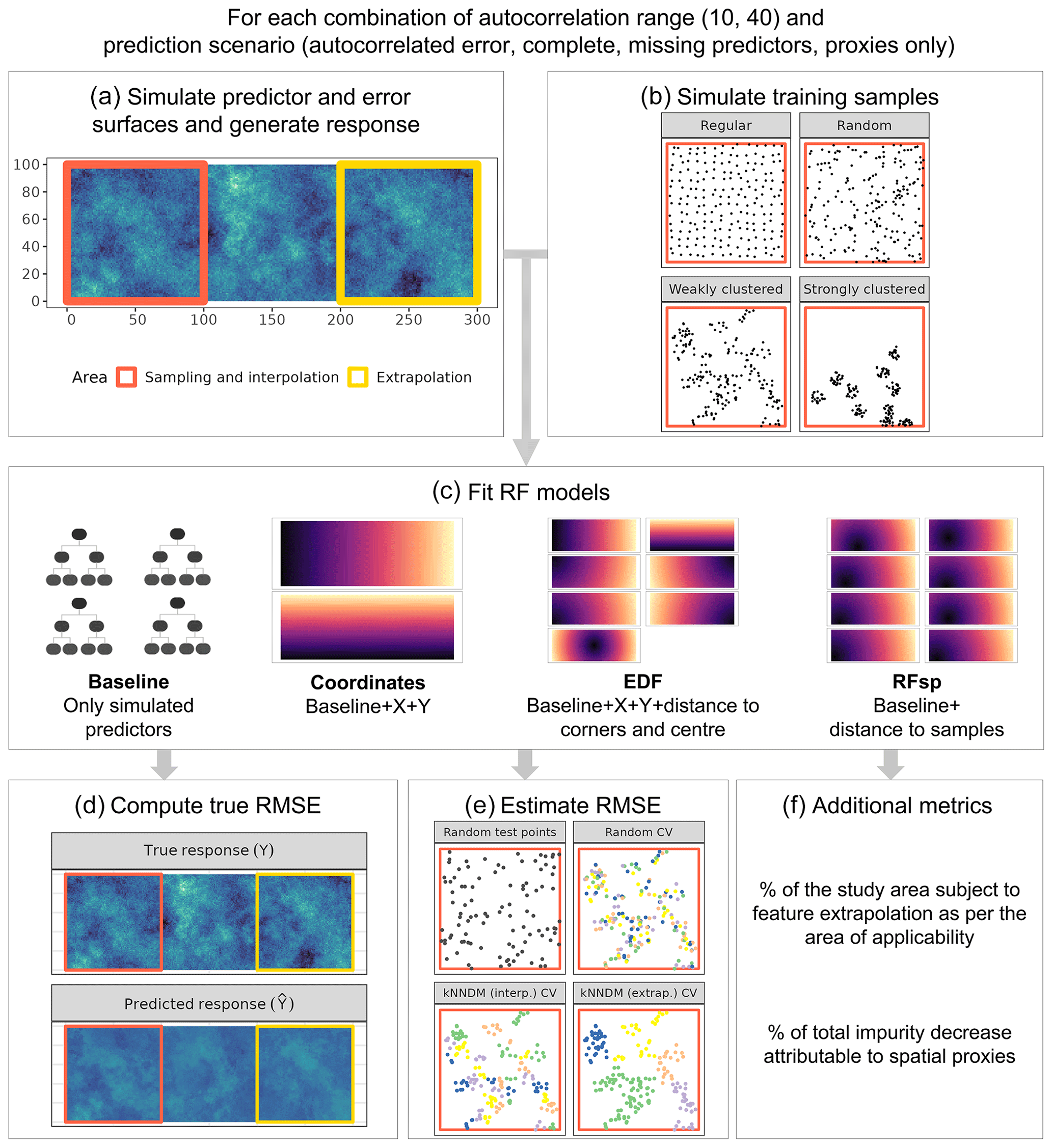
The lack of consideration of space in ML models has motivated researchers to try to find ways to account for spatial autocorrelation to improve model performance. One straightforward approach is to add spatial proxies as predictors to the ML model without any modifications being made to the algorithm. We define spatial proxies as a set of spatially indexed variables with long or infinite autocorrelation ranges that are not causally related to the response. We use the term “proxy” since these predictors act as surrogates for unobserved factors that can cause residual autocorrelation, such as missing predictors or an autocorrelated error term. The most prevalent type of proxy is coordinates, where either geographical or projected coordinate fields (Fig. 1c) are added as predictors in the models (e.g. Cracknell and Reading, 2014). Other spatial-proxy approaches include Euclidean distance fields (EDFs) (Behrens et al., 2018), which, in addition to coordinates, add distance fields with different origins, such as five EDFs corresponding to the four corners and the centre of the study area (Fig. 1c). Behrens et al. (2018) explained that with EDFs, one can account for both spatial autocorrelation and non-stationarity using the partition of the geographical space introduced by EDFs and its interaction with environmental predictors. Finally, Hengl et al. (2018) proposed random forest spatial prediction (RFsp), which adds distance fields to each of the sampling locations (Fig. 1c) – i.e. the number of added predictors equals the sample size. Hengl et al. (2018) argued that RFsp can address spatial autocorrelation, model trend, and error in a single step, mimic regression kriging while avoiding its complexity and assumptions, and benefit from the ability of RFs to fit complex relationships between the response and predictors.

Figure 1 Workflow of the simulation study.

While spatial proxies, especially coordinates, have been widely used in the literature (e.g. Walsh et al., 2017; Wang et al., 2017; de Hoogh et al., 2018), evidence exploring their suitability in different prediction settings is fragmented and limited. In our literature review, we identified three factors that could affect the effectiveness of spatial proxies: (1) the model's objective, (2) the strength of the residual spatial autocorrelation, and (3) the sample distribution.

In relation to the first factor, the objective of the model, we can distinguish between the following: interpolation, where there is a geographical overlap between the sampling and prediction areas; extrapolation or spatial-model transfer, where the model is applied to a new disjoint area; and predictive inference, where knowledge discovery is the main focus. Regarding interpolation, several studies indicate that when samples cover the entire prediction area, the addition of spatial proxies to RFs may be beneficial in terms of enhancing predictive accuracy, and they might outperform geostatistical or hybrid methods (Behrens et al., 2018; Hengl et al., 2018; Saha et al., 2023). The use of spatial proxies for extrapolation remains unexplored but appears to be problematic: since spatial representation is introduced via predictors and the prediction area is, by definition, different from the sampling area, feature extrapolation will occur when spatial proxies are used, which is problematic for models with poor extrapolation ability, such as RFs (Meyer and Pebesma, 2021; Hengl et al., 2018). Finally, regarding predictive inference, the inclusion of spatial proxies has been discouraged. Meyer et al. (2019) showed how spatial proxies typically rank highly in variable-importance statistics in RF models, especially when they lead to overfitting. Following this, Wadoux et al. (2020a) discussed how high-ranking proxies could hinder the correct interpretation of importance statistics for the rest of predictors, undermining the possibility of deriving hypotheses from the model and hampering residual analysis.

The second factor is residual autocorrelation, which typically arises when a relevant predictor is not available for modelling because it is either unmeasured or unknown or because the error term is autocorrelated (Dormann et al., 2007). Since the goal of introducing spatial proxies is to account for residual autocorrelation, better performance of models with spatial proxies is expected when residual dependencies are strong. This intuition is confirmed by the results of Saha et al. (2023), who showed that RFs with spatial proxies, especially those adding a large number of proxy predictors (such as RFsp), were especially useful when the covariate signal-to-spatial noise ratio was low (i.e. when there was a large autocorrelated error term compared to the covariate signal) but led to poor results when the spatial error was small. Nonetheless, whether proxies can address different sources of residual autocorrelation (e.g. missing predictors or autocorrelated error), as well as the influence of the strength of their spatial structure, remains to be studied.

The third factor is the sampling pattern, with clustered samples frequently being argued as potentially problematic (Cracknell and Reading, 2014; Hengl et al., 2018; Meyer et al., 2019). Indeed, the problem with clustered data is similar to that of spatial-model transferability: even if the sampling and prediction areas coincide, there will be some regions not covered by the training data, and, therefore, spatial extrapolation will occur to some degree. Cracknell and Reading (2014) showed that using coordinates with clustered data led to implausible results with significant artefacts. Hengl et al. (2018) warned about using RFsp with clustered data, which can result in feature extrapolation for a subset of the area (i.e. predicting values of spatial proxies that are not included in the training data). Meyer et al. (2019) added that including highly autocorrelated variables, such as coordinates with clustered samples, can result in spatial overfitting. In spite of this evidence, the effect of the sampling design has only been explored in specific case studies, and a systematic evaluation is still missing.

In addition to the factors influencing the suitability of spatial proxies, it is important to have validation methods to empirically assess whether a spatial-proxy approach is appropriate for a given prediction task. To our knowledge, the only evidence regarding this point is that from Meyer et al. (2019), who showed that spatial overfitting with highly autocorrelated variables was only detected when using an appropriate validation strategy. Amongst validation methods, probability test sampling is the preferred approach as it offers unbiased estimates (Wadoux et al., 2021) that can be used for model selection. Unfortunately, independent test samples are rarely available in the field of environmental sciences, and alternative validation methods, such as cross-validation (CV), must be used. While standard CV methods that assume independence between train and test data, such as leave-one-out and k-fold CV, are known to offer good accuracy estimates for spatial interpolation with regular and random samples (Wadoux et al., 2021; Milà et al., 2022; Linnenbrink et al., 2023), they generally lead to overoptimistic estimates for spatial-model transfer and interpolation with clustered samples. Several spatial CV methods have been proposed to address the limitations of standard validation approaches (Roberts et al., 2017; Ploton et al., 2020; Kattenborn et al., 2022), including CV based on spatial blocking (Wenger and Olden, 2012; Valavi et al., 2019), buffering (Telford and Birks, 2009; Le Rest et al., 2014), and clustering (Wang et al., 2023), as well as sampling-intensity-weighted CV and model-based geostatistical approaches (de Bruin et al., 2022). Among these, CV methods that consider the prediction objective of the model, such as k-fold nearest neighbour distance matching (kNNDM) CV (Linnenbrink et al., 2023), are especially interesting because they have the potential to determine whether proxies are useful for different prediction objectives, i.e. interpolation vs. extrapolation.

As an alternative to modelling with spatial proxies, other methods that do involve algorithmic modifications have been proposed, including mixed-effects tree-based models that account for correlated data (Hajjem et al., 2011, 2014), spatially aware resampling methods (Li et al., 2019), and geographically weighted ML algorithms (Georganos et al., 2021; Zhan et al., 2017). Among these, the generalized-least-squares-style random forest (RF–GLS) model recently proposed by Saha et al. (2023) is especially interesting because it relaxes the independence assumption of the RF model by accounting for spatial dependencies in several ways: (1) using a global dependency-adjusted split criterion and node representatives instead of the classification and regression tree (CART) criterion used in standard RF models; (2) employing contrast resampling rather than the bootstrap method used in a standard RF model; (3) and applying residual kriging with covariance modelled using a Gaussian process framework (Saha et al., 2023). In their simulations, Saha et al. (2023) showed how RF–GLS outperformed RFs with and without spatial proxies; however, their simulations did not reflect the typical characteristics of environmental applications as they only explored random sampling designs and did not use spatially structured predictors.

Even though their strengths and weaknesses have been discussed, spatial proxies continue to be widely used, and coordinates are typically added to the set of predictors by default without further consideration. Hence, a comprehensive investigation is required to complement the fragmented evidence that is currently mostly available from case studies. In this work, we investigate several RF models with spatial proxies, i.e. coordinates, EDFs, and RFsp, with the following objectives:

1. to assess the suitability of spatial proxies depending on different factors: the modelling objective (interpolation vs. extrapolation), the strength of the residual spatial autocorrelation, and the sampling pattern.

2. to investigate which validation methods can be used as a model selection tool to empirically assess the suitability of spatial proxies and select the most appropriate proxy configuration.

3. to provide guidance to practitioners regarding the use of spatial proxies in real-world applications.

We address the first two objectives in a simulation study, whereas for the third objective we carry out two case studies where we model air temperature and particulate air pollution in Spain. We further compare and discuss the findings in the context of the recently developed RF–GLS to benchmark the performance of this alternative modelling approach.

2 Methods

2.1 Simulation study

We designed a simulation study on a virtual 300×100 grid to assess, across different prediction settings, the suitability of RF regression models using three different types of spatial proxies: coordinates, EDFs, and RFsp (Fig. 1). Within the grid, two separate areas were defined (Fig. 1a): the sampling area, from which observations were sampled and which coincided with the interpolation prediction area, and the extrapolation prediction area, used to evaluate spatial-model transferability. The simulation consisted of the following steps:

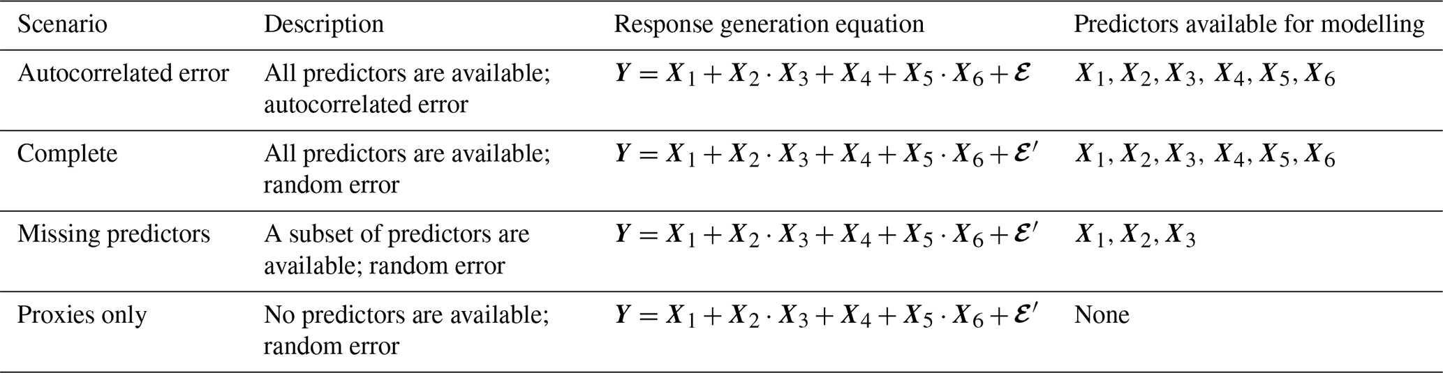
1. We generated predictor and response surfaces (Fig. 1a) according to the different scenarios described in Table 1. These were (1) “autocorrelated error”, where residual autocorrelation is expected due to a spatially autocorrelated error term; (2) “complete”, where no spatial autocorrelation is expected, and, therefore, spatial proxies are assumed to be irrelevant; (3) “missing predictors”, where residual autocorrelation is present due to missing predictors; and finally (4) “proxies only”, where no predictors are available for modelling and only proxies are used. To generate the surfaces, unconditional sequential Gaussian simulation (Gebbers and de Bruin, 2010) was used to generate six independent predictor fields, X, with a mean of 0 and a spherical variogram with a sill value of 1, a nugget value of 0, and a range of 10 or 40 (see examples in Fig. A1), which were to be used in response Y generation. Additionally, we simulated autocorrelated error surfaces (𝓔; a random field with a mean of 0 and a spherical variogram with a sill value of 1, a nugget value of 0, and a range of 25) and random error surfaces (𝓔^′; standard Gaussian) (Fig. A1). We generated response surfaces using the equations in Table 1.

2. We simulated four sets of training points in the sampling area (Fig. 1b), each with a sample size of 200, following different distributions: regular samples were drawn by adding random noise (uniform distribution with parameters $U(-\mathrm{2},\mathrm{2})$) to a regular grid, random samples were simulated via uniform random sampling, clustered samples were obtained by simulating 25 (weak clustering) or 10 (strong clustering) randomly distributed parent points as a first step and 7 (weak) or 19 (strong) offspring points within an eight-unit (weak) or six-unit (strong) buffer around each parent.

3. For each set of samples, we extracted the corresponding values of the response and predictors, deleted duplicate observations (i.e. two or more points intersecting the same cell), and fitted a baseline RF model using predictors according to the corresponding scenario (Table 1). We also fitted coordinates, EDFs, and RFsp models (see Introduction for details), which included the predictors from the baseline model plus the spatial proxies (Fig. 1c). We kept the number of trees at a constant value of 100 and tuned the hyperparameter mtry using out-of-bag samples and an equally spaced grid with a length of 5, ranging from 2 to the maximum number of predictors.

4. We used each of the fitted models to compute predictions for the entire area and calculated the “true” root mean square error (RMSE) by comparing the simulated and predicted response surfaces in all interpolation and extrapolation areas separately (Fig. 1d). In the baseline model for the “proxy only” scenario, where no predictors were available, the mean of the response in the training data was used as a constant prediction. The expected minimum possible RMSE for the second through fourth scenarios was equal to 1 (standard deviation of the random error), whereas it was equal to 0 for the “autocorrelated error” scenario as the error could potentially be explained by the proxies.

5. Since the true RMSE is unknown in real-world applications, we also estimated the RMSE using additional validation methods (Fig. 1e). First, a probability sample containing 100 random test points was drawn and used to estimate the RMSE in the interpolation and extrapolation areas separately. Moreover, 5-fold random CV and 5-fold kNNDM CV were used to estimate the RMSE. Briefly, kNNDM CV is a prediction-oriented method that provides predictive conditions in terms of geographical distances during CV that are similar to those encountered when using a model to predict a defined area (Linnenbrink et al., 2023; Milà et al., 2022). kNNDM CV has been shown to provide a better estimate of map accuracy than random k-fold CV when used with clustered samples, while returning fold configurations equivalent to random k-fold CV for regularly and randomly distributed samples. Estimation of the RMSE was done globally to account for the different fold sizes in kNNDM CV (Linnenbrink et al., 2023) – i.e. we stacked all predictions in the different folds and computed the RMSE from all samples simultaneously, rather than computing the RMSE within each fold and then averaging the results. As kNNDM CV is dependent on the prediction objective, two different kNNDM CV configurations were used to estimate the RMSE in the interpolation and extrapolation areas (Fig. 1e).

6. We computed two additional metrics to understand the feature extrapolation potential and the variable importance of spatial proxies (Fig. 1f). We calculated the percentage of the study area subject to feature extrapolation according to the area of applicability (AOA) (Meyer and Pebesma, 2021) using all training samples. The AOA is defined as the area with feature values similar to those in the training data and is computed based on distances in the predictor space. Unlike feature extrapolation metrics based on variable ranges or convex hulls, the AOA takes into account predictor sparsity within the predictor range and weights variables according to their importance in the model. Regarding variable importance, we used the mean decrease impurity method (Breiman, 2002) to quantify the percentage of the total average impurity decrease attributable to spatial proxies.

Table 1 Description of the scenarios in the simulation study. 𝓔 corresponds to a spatially autocorrelated error, while 𝓔^′ represents a random error.

We ran 100 iterations of each simulation configuration – i.e. we fitted a total of 100 iterations × 4 prediction scenarios × 2 autocorrelation ranges × 4 sample distributions × 4 model types, resulting in 12 800 models (without counting the CV fits). We analysed the results of the simulations by examining the distributions of (1) the true RMSE, (2) the percentage of the study area subject to feature extrapolation, (3) the percentage of variable importance attributable to spatial proxies, and (4) the estimated RMSE for each combination of simulation parameters and model type.

2.2 Comparison of spatial proxies with RF–GLS

As an alternative to spatial-proxy approaches, we also tested the performance of the RF–GLS model recently proposed by Saha et al. (2023). This model is an extension of the RF model and relaxes its independence assumption by accounting for spatial dependencies in several ways (see Introduction for more details). To test the performance of RF–GLS, we included it in the set of candidate models, along with the baseline and the three spatial-proxy models used in the simulations presented in Sect. 2.1, used it to predict the entire area, and computed the “true” RMSE in the interpolation and extrapolation areas by comparing the simulated and predicted response surfaces.

2.3 Case studies

We modelled annual average air temperature and fine particulate air pollution for continental Spain in 2019 to examine the use of RF models with spatial proxies in real-word examples. For the first case study, we collected daily average air temperature data using the application programming interface of the Agencia Estatal de Meteorología, calculated station-based annual averages, and retained 195 stations with a temporal coverage of 75 % or higher (Fig. 2). For the second case study, we collected data on concentrations of particulate matter with a diameter of 2.5 µm or less (PM_2.5) from the Ministerio para la Transición Ecológica y el Reto Demográfico. For PM_2.5 stations with an hourly resolution, we first computed daily averages whenever at least 75 % of the observations for a given day were available. Then, we computed the annual averages and retained 124 stations with an annual temporal coverage of 75 % or higher (Fig. 2).

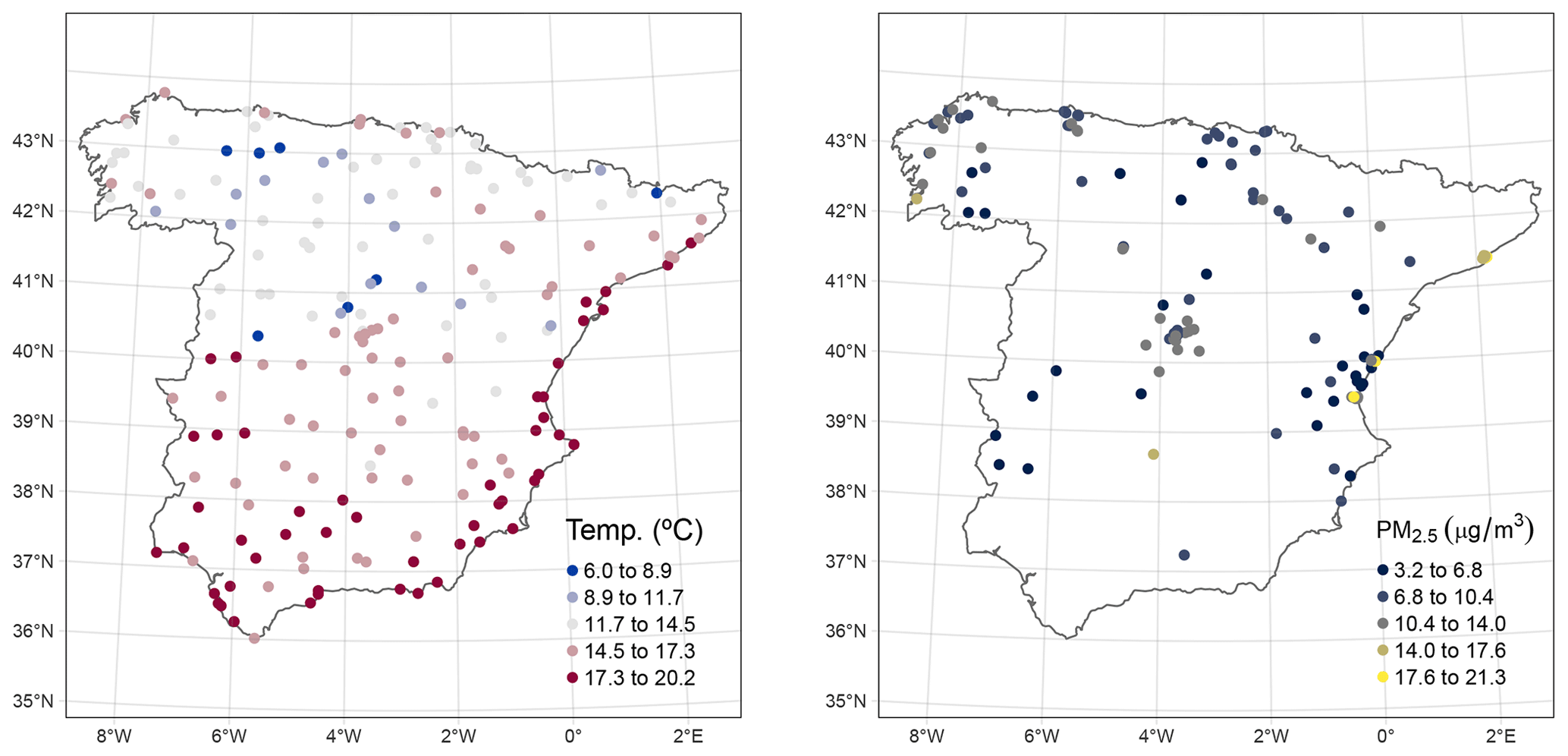
Figure 2 Spatial distribution of the reference station data for the air temperature and air pollution case studies.

We generated a 1 km×1 km grid covering continental Spain as a prediction area. Details of all data used for predictor generation are included in Table A1, while the code for all pre-processing steps and processed data used for modelling are publicly available (see the “Code and data availability” section). Briefly, we collected a digital elevation model (DEM), an impervious-density product, gridded population counts, land cover data, coastline geometries, road geometries by type, a satellite-based Normalized Difference Vegetation Index (NDVI) from the MODIS/Aqua 16 d NDVI product (MYD13A1) and 8 d Land Surface Temperature product (LST; MYD11A2), annual nighttime light (NTL) data from VIIRS, and European atmospheric composition reanalyses for PM_2.5 from the Copernicus Atmosphere Monitoring Service (CAMS). We derived population density from the georeferenced population data, computed the percentages of different land cover classes (urban, industrial, agricultural, and natural) in each 1 km grid cell, measured distances from each cell centroid to the nearest coastline, calculated primary-road density (highway and primary roads) and secondary-road density (all other vehicle roads) as the length of the road segments within each 1 km×1 km cell, and computed annual average composites of the NDVI, LST, and CAMS data. We regridded predictors to the target 1 km×1 km grid using bilinear interpolation (downscaling) or averaging (upscaling) depending on the source resolution. We extracted predictor values at the station locations for subsequent modelling.

Unlike in the simulation study, in these real-world case studies the strength of the spatial autocorrelation of the response and the sample spatial distribution were unknown. To understand how these factors may affect the performance of the different models, we performed an exploratory analysis for each response. First, we assessed the spatial distribution of the monitoring stations using exploratory spatial-point-pattern analyses. Namely, we estimated the empirical $\widehat{G}$, $\widehat{F}$, and $\widehat{K}$ functions; Monte Carlo simulations (n=99) were used to construct simultaneous envelopes to assess the departure from complete spatial randomness (Baddeley et al., 2015). Secondly, we computed empirical variograms of the response variables to assess the strength of the autocorrelation.

For each response, we considered two different sets of variables to be included in the models. First, a naive model was used, where only one predictor, known a priori to be a strong driver of the response, was included – elevation for temperature and primary-road density for PM_2.5. Second, a complete model was used, where a much more comprehensive set of predictors were included (see list in Table A1). Our motivation for the naive model was to examine whether spatial proxies could help explain residual spatial autocorrelation due to missing predictors and therefore be used in predictor scarcity settings. Similar to the simulation study, we used an RF regression baseline model with the selected predictors, as well as coordinates, EDFs, and RFsp as additional proxy predictors. We fixed the number of trees to 300 and tuned the parameter mtry using out-of-bag samples and an equally spaced grid of length 10, ranging from 1 to the maximum number of predictors. Using the same methods as in the simulation study, we estimated the performance by estimating the RMSE and R² using 10-fold random CV and kNNDM CV (no probability test samples were available), calculated the percentage of the study area subject to extrapolation, and estimated the relative importance of spatial proxies. We plotted the predicted surfaces and presented the computed statistics. We assessed residual spatial autocorrelation using empirical variograms of the residuals from each model to evaluate whether spatial dependencies in the data had been captured.

2.4 Implementation

Our analyses were carried out in R version 4.2.2 (R Core Team, 2022) using several packages: sf (Pebesma, 2018) and terra (Hijmans, 2022) for spatial-data management; caret (Kuhn, 2022), ranger (Wright and Ziegler, 2017), RandomForestsGLS (Saha et al., 2022), and CAST (Meyer et al., 2023) for spatial modelling; gstat (Pebesma, 2004) for random-field simulation; and ggplot2 (Wickham, 2016) and tmap (Tennekes, 2018) for graphics and cartographic representations. Additional packages were used for other minor tasks.

3 Results

3.1 Simulation study

3.1.1 Suitability of spatial proxies

The prediction objective was a clear determinant of the suitability of spatial proxies. When predicting in the extrapolation area (Fig. 3), baseline models always outperformed spatial-proxy models, regardless of other parameters, highlighting the inability of proxies to successfully be transferred to new areas that differ from those where they were trained. This was supported by feature extrapolation statistics of proxy models (Fig. A2), which indicated that a very large part (or even all) of the extrapolation area had feature values not covered by the training data.

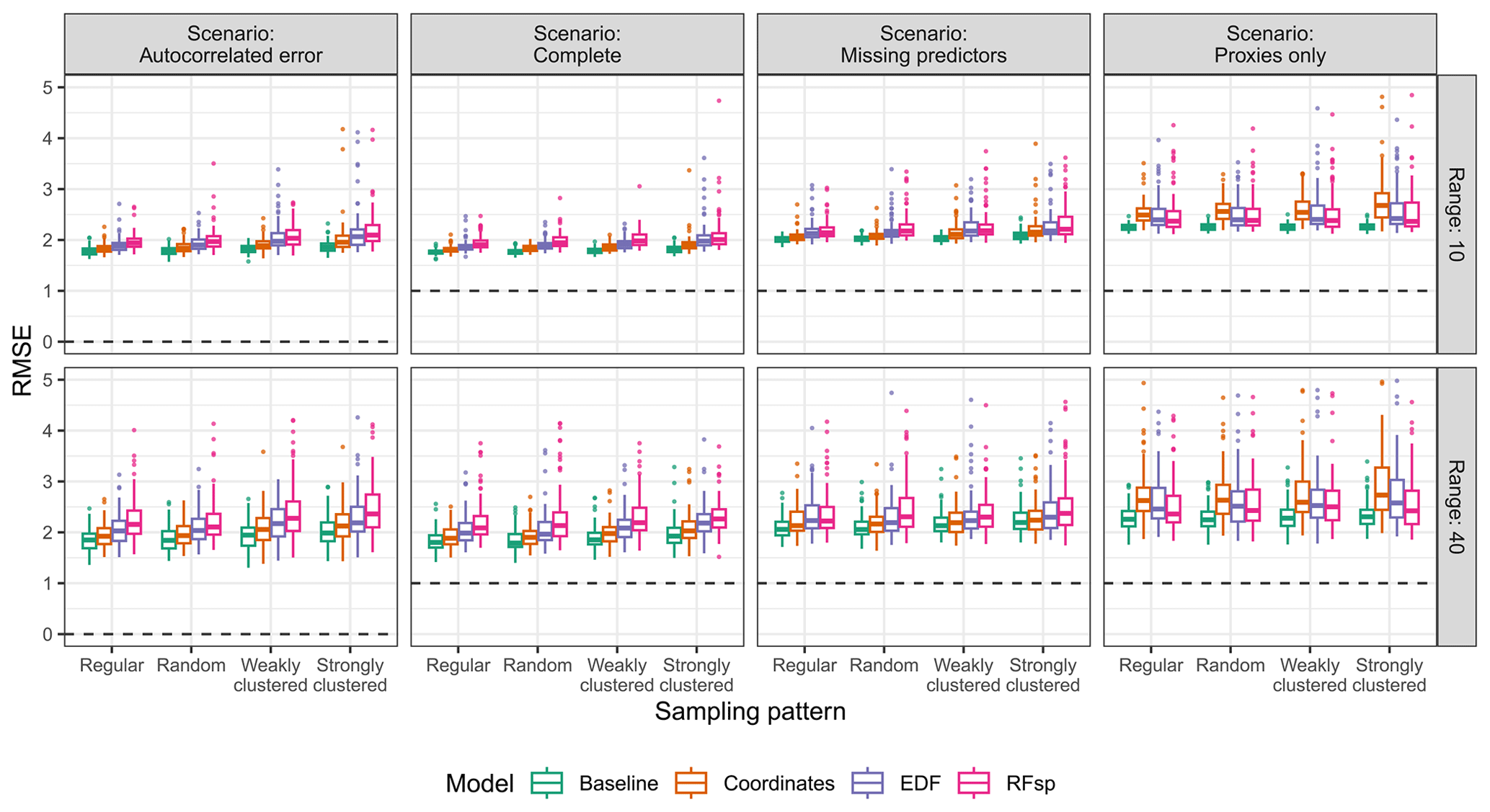
Figure 3 True RMSE in the extrapolation area of each model type, based on the scenario, autocorrelation range, and sampling pattern. The dashed lines indicate the minimum possible RMSE for each scenario. The RMSE for the baseline model in the “proxies only” scenario uses a constant prediction value, calculated as the average response value in the training data. Outliers larger than 5 are not shown for visualization purposes.

The suitability of spatial proxies for interpolation was more complex and depended on a series of additional factors, including the strength of the residual autocorrelation (Fig. 4). In the “complete” scenario, where residual spatial autocorrelation was not expected, models with spatial proxies yielded RMSE values that were similar or larger than those of the respective baseline models. On the other hand, in scenarios where residual autocorrelation was expected due to either an autocorrelated error term or missing predictors, models with spatial proxies showed smaller errors in many instances. Regarding the extent of the spatial autocorrelation, spatial-proxy models offered more benefits in situations in which the spatial structure of the predictors and response, expressed as the autocorrelation range, was stronger.

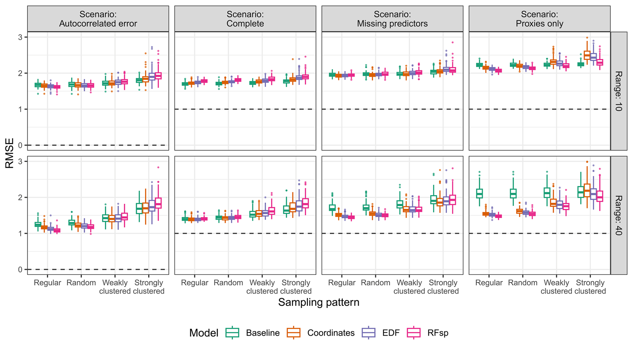
Figure 4 True RMSE in the interpolation area of each model type, based on the scenario, autocorrelation range, and sampling pattern. The dashed lines indicate the minimum possible RMSE for each scenario. The RMSE for the baseline model in the “proxies only” scenario uses a constant prediction value, calculated as the average response value in the training data. Outliers larger than 3 are not shown for visualization purposes.

The suitability of spatial proxies for interpolation was also influenced by the sampling pattern. With random and regular samples (Fig. 4), adding spatial proxies tended to decrease errors in scenarios where residual spatial autocorrelation was expected, while yielding results comparable to or only slightly worse than those in the “complete” scenario. This is connected to the low levels of feature extrapolation observed for random and regular sampling patterns (Fig. A3) – since the samples covered the entire extent of the interpolation area, adding spatial proxies did not impact feature extrapolation, which remained low. Nonetheless, when samples were clustered, adding spatial proxies increased feature extrapolation (Fig. A3), leading to models with a generally larger RMSE compared to that of baseline models, except in cases where residual spatial autocorrelation was strong and the sampling pattern was only weakly clustered (e.g. the “missing predictors” scenario with weakly clustered samples and a range of 40, shown in Fig. 4). Finally, interpolation models using only spatial proxies as predictors performed nearly as well as models with all predictors (“complete” scenario) or a subset of predictors (“missing predictors” scenario), provided the samples were regularly or randomly distributed and the autocorrelation range was set to 40 (Fig. 4).

Comparing the different types of spatial proxies, RFsp tended to give worse results than coordinates when its use was inappropriate for either interpolation or extrapolation. Nonetheless, together with EDFs, it also yielded the largest gains when the use of proxies was beneficial. We attribute this to the larger number of spatial-proxy predictors in RFsp and EDF models compared to coordinates, leading to a higher proxy feature importance (Fig. A4). The feature importance of spatial proxies was larger for clustered samples compared to regular and random patterns, as well as for the long autocorrelation range (Fig. A4).

3.1.2 Validation methods for proxy selection

In the extrapolation area and the “autocorrelated error” scenario, random 5-fold CV not only severely underestimated the true RMSE but also systematically and erroneously suggested that models with proxies had a similar or superior performance compared to that of baseline models (Fig. 5). On the other hand, both probability test samples and kNNDM CV correctly ranked models according to their true RMSE. Results for the extrapolation area in the rest of scenarios are available in Figs. A5–A7 and show similar patterns.

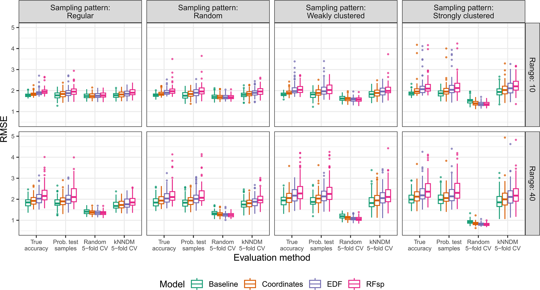
Figure 5 True and estimated RMSEs in the extrapolation area and the “autocorrelated error” scenario, based on the evaluation method, autocorrelation range, and sampling pattern. Outliers larger than 5 are not shown for visualization purposes.

In the interpolation area and the “autocorrelated error” scenario (Fig. 6), all validation methods correctly ranked models with regular and random sampling patterns. However, with clustered sampling patterns, random k-fold CV indicated that models with spatial proxies were superior when, in fact, they were similar or worse. Similar results were observed in the rest of the scenarios in the interpolation area (Figs. A8–A10).

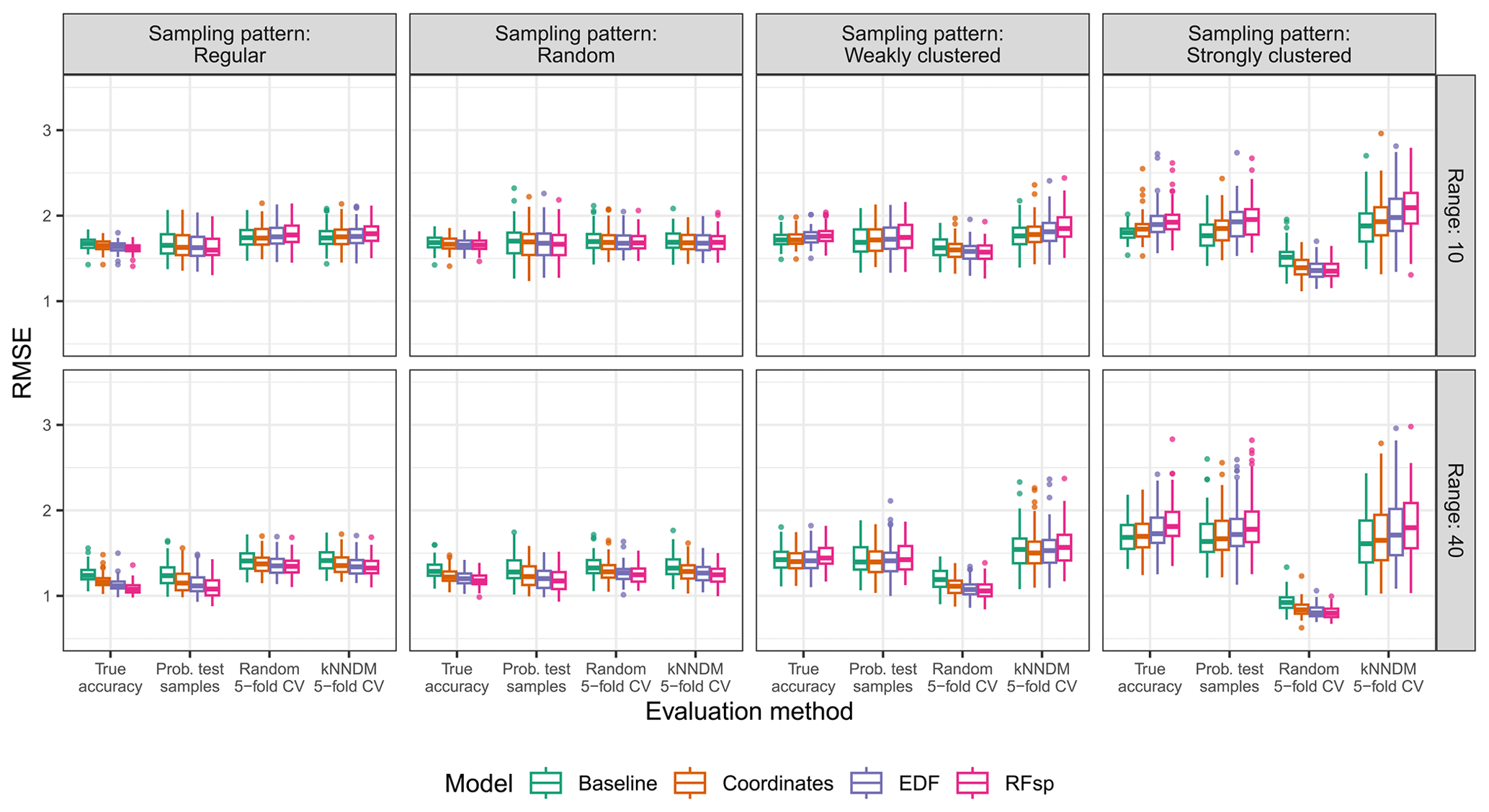
Figure 6 True and estimated RMSEs in the interpolation area and the “autocorrelated error” scenario, based on the evaluation method, autocorrelation range, and sampling pattern. Outliers larger than 3.5 are not shown for visualization purposes.

3.1.3 Comparison of spatial proxies with RF–GLS

The RF–GLS model outperformed or was on a par with the best-performing standard RF model with and without proxies for all parameter combinations in both the interpolation (Fig. 7) and extrapolation (Fig. A11) areas of the simulation study. The most relevant performance gains when comparing RF–GLS to RFs with and without proxies were observed in the “autocorrelated error” scenario for the interpolation area with regular and random samples, where the RMSE was substantially lower.

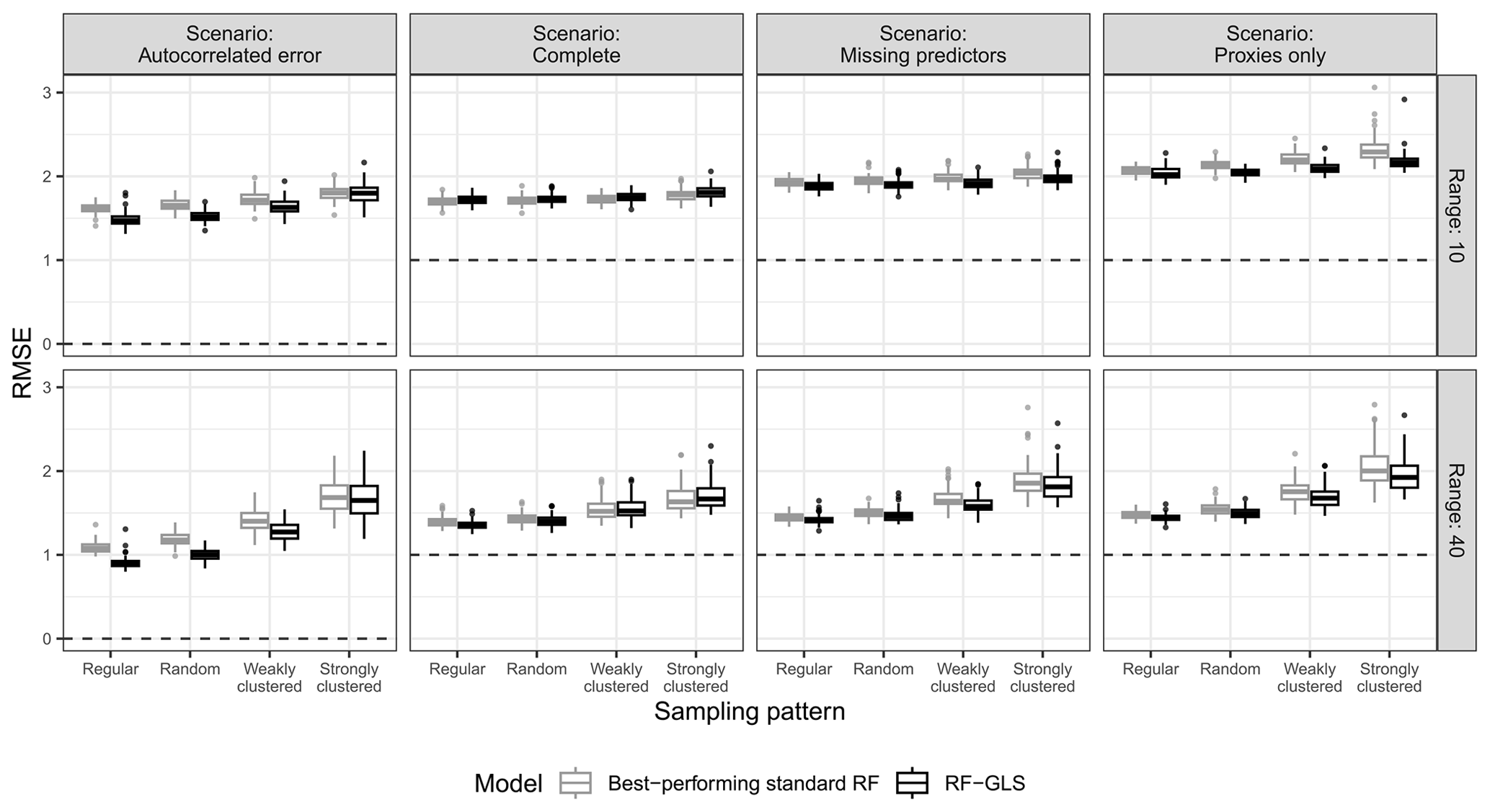
Figure 7 True RMSE in the interpolation area of the best-performing standard RF for each parameter combination (i.e. the standard RF model with/without proxies that has the lowest median RMSE) and RF–GLS, based on the prediction scenario, spatial-autocorrelation range, and sampling pattern. The dashed line indicates the minimum possible RMSE for each scenario.

3.2 Case studies

Air temperature meteorological stations were well spread over the study area (Fig. 2), and the point pattern exploratory analysis did not suggest a major departure from complete spatial randomness, although there was some evidence of a regular pattern (Fig. A12). Aligned with these results, kNNDM CV generalized to a random 10-fold CV (Fig. A13).

Results for the naive temperature model indicated substantial gains in performance when using spatial proxies, yielding only slightly worse results than those of complete models (Table 2). Performance of all complete models was similar. Feature extrapolation was similar across all cases and covered less than 10 % of the study area. We detected strong spatial autocorrelation in the response and residuals of the naive baseline model, which mostly disappeared when adding the whole set of predictors and/or spatial proxies (Fig. A14). Adding spatial proxies to the naive baseline model, which only included a DEM, resulted in different patterns and smoother predicted surfaces (Fig. 8). When comparing naive models with spatial proxies to complete models, spatial patterns were quite similar, although the latter exhibited more local variation. Differences between maps derived from complete models with and without proxies were minor.

Table 2 Results of the temperature case study. Subscripts for RMSE and R² indicate the type of 10-fold CV used to compute the statistics. Statistics generated via random 10-fold CV are computed as the mean (SD) of the statistics calculated for each fold, while statistics generated via kNNDM CV are computed by stacking all observed and predicted values (see Methods).

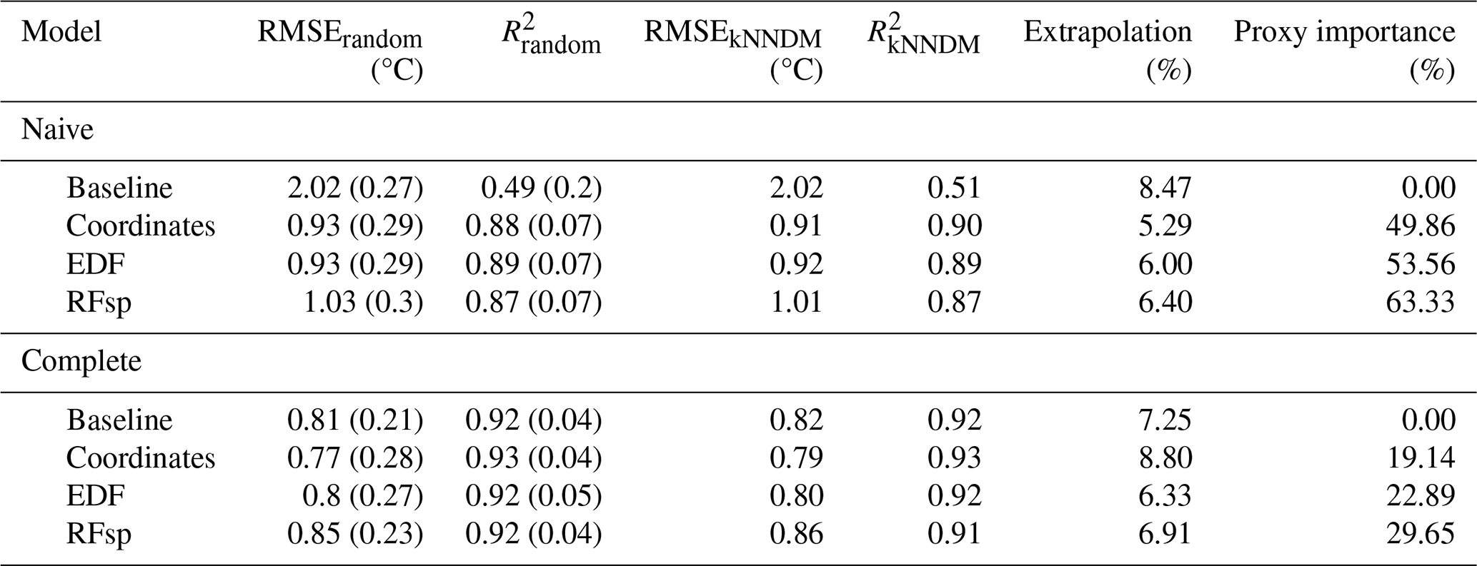
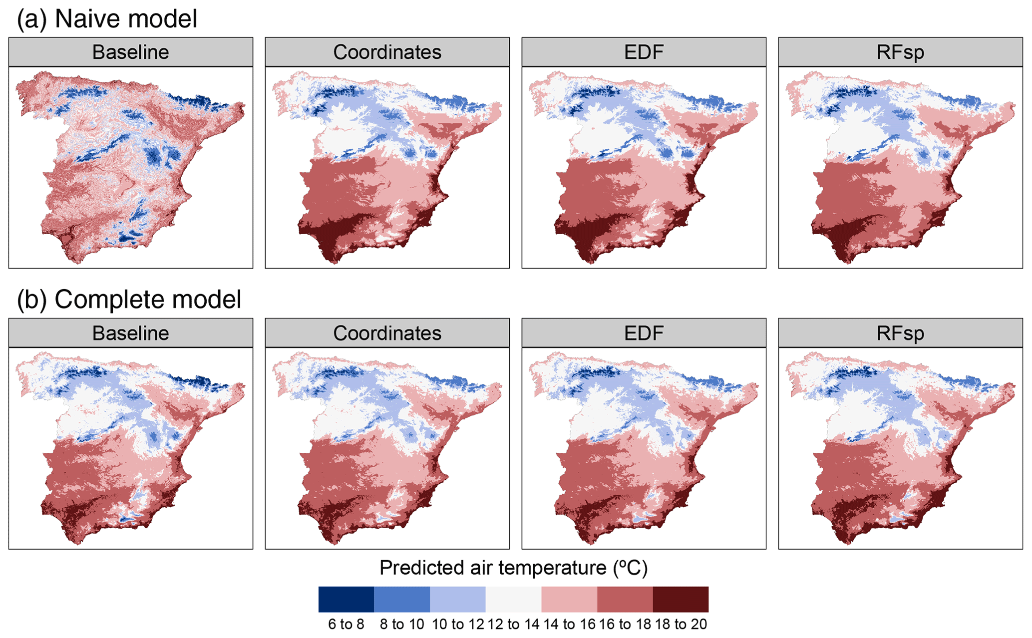
Figure 8 Predicted air temperature using (a) naive predictors (DEM only) and (b) complete predictors, based on model type.

The distribution of PM_2.5 stations visually appeared to be spatially clustered (Fig. 2), which was confirmed by the exploratory spatial-point-pattern analysis, showing a clear departure from complete spatial randomness (Fig. A15). Reflecting this clustering pattern, the resulting kNNDM CV had a distinct spatial configuration (Fig. A16).

According to random 10-fold CV, the estimated performance of the naive baseline model in terms of R² was almost null, but it improved substantially when adding spatial proxies. Nonetheless, when using kNNDM CV, the estimated performance was similarly null across all cases (Table 3). The estimated RMSEs of complete models were still lower when using random CV compared to kNNDM CV; however, statistics across the different model types were much more similar. Feature extrapolation was the highest in naive models, where proxies had a larger importance, leading to mapping artefacts that were especially evident in the coordinates model (Fig. 9). Unlike in the temperature case study, the predicted surfaces of naive models with proxies and complete models were very different, suggesting that the added geographical predictors did not successfully account for the missing predictors. Prediction maps for complete models with different spatial proxies were much more similar. Inspection of the empirical variograms for the response and residuals of the naive baseline model indicated the presence of spatial autocorrelation, which was weaker than that for air temperature and disappeared in complete and spatial-proxy models (Fig. A17).

Table 3 Results of the PM_2.5 case study. Subscripts for RMSE and R² indicate the type of 10-fold CV used to compute the statistics. Statistics generated via random 10-fold CV are computed as the mean (SD) of the statistics calculated for each fold, while statistics generated via kNNDM CV are computed by stacking all observed and predicted values (see Methods).

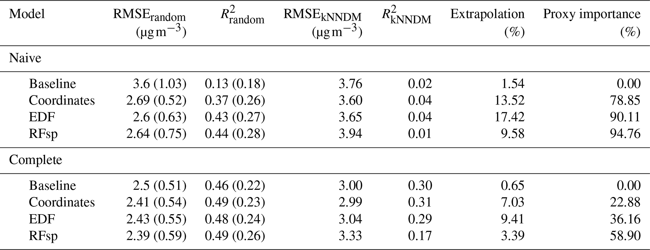
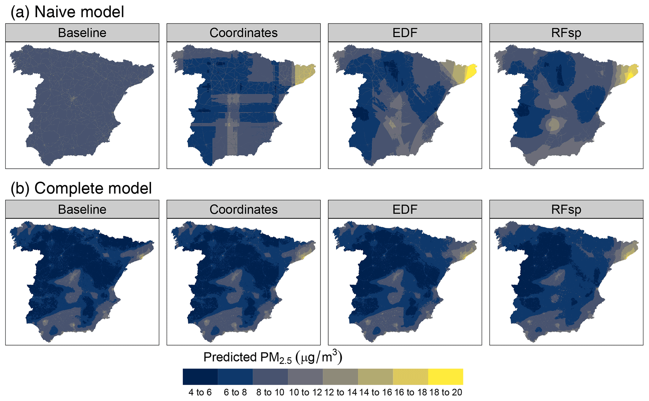
Figure 9 Predicted PM_2.5 using (a) naive predictors (primary-road density only) and (b) complete predictors, based on model type.

4 Discussion

Our first objective was to assess the suitability of spatial proxies based on the modelling objective, the strength of the residual spatial autocorrelation, and the sampling pattern. Regarding the modelling objective, we found that using an RF with spatial proxies is never beneficial when the goal is spatial-model transfer to a new area. Adding spatial proxies that identify specific locations of the sampling area to the predictor set inevitably leads to feature extrapolation in the new area as values of proxy predictors will be completely different. Additionally, when proxies are used as node-splitting variables in the RF model, we end up only using observations located on the edge of the sampling area, regardless of their distance to the new prediction area. This contrasts with methods such as RF–GLS or regression kriging, which can account for the autocorrelation decay with increasing distances. Therefore, these variables should not be used for prediction in new geographical areas, and the focus should be placed on causal predictors.

For interpolation purposes, however, proxies may be beneficial depending on additional factors. We discovered that one of the conditions making the inclusion of spatial proxies in RF models beneficial is the presence of residual autocorrelation due to missing predictors or an autocorrelated error. These potential benefits arise from the ability of spatial proxies to account for residual spatial autocorrelation (Hengl et al., 2018; Behrens et al., 2018), as our results confirmed in terms of both improved performance and removed residual autocorrelation, especially when using a larger number of proxies (EDFs or RFsp). However, in complete models with no residual autocorrelation, the similar or occasionally worse performance is caused by adding an irrelevant set of predictors that act as noise for the model. Unlike regression kriging, where spatial autocorrelation is modelled in the residuals and its absence results in a pure nugget effect, i.e. a flat variogram leading to an ordinary least squares estimation (Hengl, 2007), in an ML model, irrelevant proxies are still included. Even though RFs are fairly robust to the addition of irrelevant predictors (Kuhn and Johnson, 2019), a decrease in performance was sometimes observed. In addition to the presence of spatial autocorrelation, the strength of the spatial structure (as defined by the autocorrelation range) was also important. When ranges become shorter, we get closer to the independence assumption of a non-spatial model, and, thus, proxies start to become irrelevant. Experiments with response variables exhibiting weaker spatial autocorrelation, such as land cover, would be interesting follow-up studies to further clarify this point.

In addition to the presence of significant spatial autocorrelation, we found that an almost necessary condition for proxies to be beneficial for interpolation is having regular or randomly distributed samples. This is not surprising since the feature extrapolation potential of spatial proxies with clustered samples has been stressed before (Meyer et al., 2019; Hengl et al., 2018; Cracknell and Reading, 2014). The more proxies used in the models, the greater the feature extrapolation. Given these results, although it is required that spatial proxies have a lower importance when used with clustered samples vs. regular or random samples, we actually observed the opposite. This is likely a sign of overfitting, where the model uses the proxies to determine the position of the sampling clusters (Meyer et al., 2019), a hypothesis supported by the differences between the estimated random CV, probability test samples, and kNNDM CV. Our results are consistent with spatial sampling recommendations for ML models, such as RFs, which suggest using designs that ensure a good spread of the most important predictors to optimize performance (Wadoux et al., 2019). Hence, spatial proxies are expected to be poorly suited for modelling with clustered samples by design. Even though our simulations indicate that weakly clustered data may sometimes also slightly benefit from spatial proxies, we recommend proceeding with caution because it is challenging to define the degree of clustering at which these proxies start to be harmful.

Our simulations allow us to give general guidelines on the adequacy of spatial proxies; however, it is important to have a way to confirm these guidelines empirically. This was the focus of the second objective, where we showed that random CV underestimates map accuracy when assessing extrapolation performance or interpolation with clustered samples, as has been shown before (Linnenbrink et al., 2023; Wadoux et al., 2021). Perhaps even more critically, random CV incorrectly ranks models in these instances, systematically favouring models with proxies even when they are not always appropriate. On the other hand, probability test samples and kNNDM CV provided correct model ranks. We think this is related to overfitting and the inability of random k-fold CV to reflect predictive conditions (Meyer and Pebesma, 2022) – in the presence of clustered sampling, adding spatial proxies may actually help the model to predict at locations geographically close to the samples, as reflected by random CV, but may fail to generalize across the entire prediction area, as measured by probability test samples and kNNDM CV.

Our additional analyses regarding the RF–GLS model proposed by Saha et al. (2023) indicate that RF–GLS performed equally as well as or better than the best-performing standard RF, both with and without spatial proxies, across all parameter configurations, which we attribute to several reasons. First, in RF–GLS, residual variability is modelled as a Gaussian process rather than with spatial-proxy predictors in the mean term, which minimizes issues with feature extrapolation and spatial overfitting arising in spatial-model transfer or interpolation with clustered samples. Furthermore, in RF–GLS, the independence assumption of the RF model is relaxed as spatial autocorrelation is accounted for during the model fitting. Finally, RF–GLS can adapt better to settings where residual spatial autocorrelation is weak or absent since the estimation of the covariance function can consider the absence of autocorrelation. Hence, we think that RF–GLS represents a step forward in creating truly spatial ML models, and it should be considered a candidate algorithm for spatial-predictions tasks.

As the third objective, we presented two case studies with distinct characteristics that reflect different real-world settings. For air temperature, stations were spread across the entire prediction area, and measurements exhibited strong spatial autocorrelation. We found that a model with only a DEM and spatial proxies managed to account for the residual spatial autocorrelation, and it performed almost as well as a much more comprehensive model that produced similar predicted surfaces. This highlights the value of spatial proxies for cost-effective predictive modelling when the conditions outlined above are met. Regarding air pollution, samples were clustered, and the autocorrelation was weaker. In both naive and complete models, spatial proxies did not improve the performance, and large differences in the CV approaches were revealed, highlighting the aforementioned risk of spatial overfitting and wrong conclusions when inappropriate validation practices are used. In the two case studies, we showed the importance of performing a comprehensive spatial exploratory analysis to determine the sample distribution and the response and residual spatial autocorrelation in the baseline model (i.e. without proxies). The results of this analysis can help us determine whether a spatial-proxy approach is advisable a priori, which can be confirmed a posteriori using model selection tools such as probability test samples or kNNDM CV.

In this study, we included a wide range of conditions typically encountered in environmental spatial modelling. Nonetheless, there are several points for future work. First, we focused on RF regression, and, while we think that our results likely extend to other ML algorithms, the extrapolation behaviour and sensitivity to irrelevant predictors differs depending on the algorithm and might limit the ability to generalize our results. Second, our analysis was based on the adequacy of spatial proxies from a prediction accuracy point of view. When using the RF model for knowledge discovery, variables with long or infinite autocorrelation ranges, such as spatial proxies, have been identified as being beyond the prediction horizon (Behrens and Viscarra Rossel, 2020; Wadoux et al., 2020b; Fourcade et al., 2018), and variable-importance statistics in models that include these variables should be interpreted with extreme caution (Meyer et al., 2019; Wadoux et al., 2020a). Third, feature selection based on an appropriate CV scheme has been shown to be helpful in discarding irrelevant features prone to overfitting that generalize poorly to new locations, such as coordinates (Meyer et al., 2019). In future work, it would be interesting to explore whether feature selection could help identify irrelevant spatial-proxy features. Fourth, we focused our investigation on the potential of spatial proxies to account for spatial autocorrelation. However, it has been suggested that coordinates and distance fields can also be useful in accounting for non-stationarity (Behrens and Viscarra Rossel, 2020), which remains to be explored. Finally, the scope of our study was limited to spatial-proxy approaches and RF–GLS; however, our analyses could be extended to consider other models proposed in the literature, e.g. models including spatial lags of the response as prediction features (Sekulić et al., 2020).

5 Conclusions

We recommend the RF model with spatial proxies in cases where all of these conditions apply: (1) the sampling and prediction areas overlap (i.e. spatial interpolation), (2) there is significant residual spatial autocorrelation due to missing predictors or an autocorrelated error term, and (3) samples are regularly or randomly distributed over the prediction area. In such cases, the addition of spatial proxies is very likely to be beneficial in terms of performance. If samples are regular or randomly distributed but no residual autocorrelation is present, the addition of spatial proxies will have little impact. Finally, in the presence of clustered samples, using spatial proxies in RF models is generally not recommended since their inclusion can degrade model performance, especially if residual autocorrelation is weak and the clustering is strong. Proxies should not be used for spatial-model transfer.

More generally, we have shown that the benefits of RFs with spatial proxies are not universal, and, therefore, they should not be taken as a default approach without careful consideration. Spatial exploratory analysis of the sample distribution and the response and residual autocorrelation is recommended as a preliminary step to evaluate the suitability of spatial proxies, while probability test samples and kNNDM CV can be used as model selection tools to confirm their suitability and choose the best set of proxies. Random k-fold CV should not be used for model selection if the objective is spatial-model transfer or if clustered samples are present since it erroneously favours models with spatial proxies. RF–GLS should be considered a candidate modelling algorithm for spatial-prediction tasks.

Appendix A: Additional figures and tables

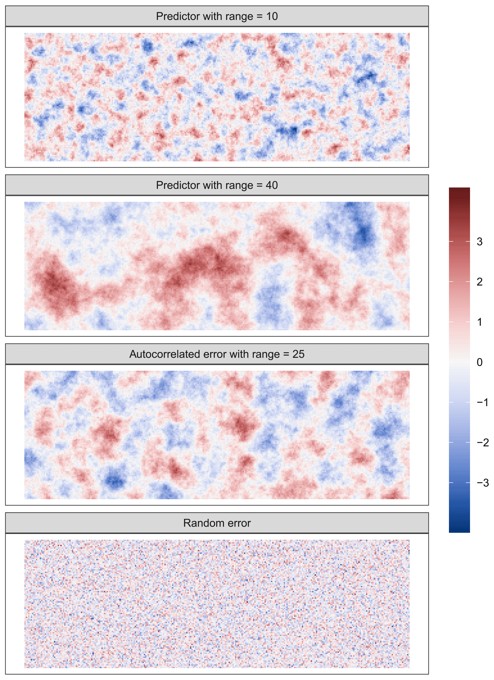
Figure A1 Example realizations of random fields used in the simulation study. All random fields have a mean of 0. Predictor and autocorrelated error surfaces were generated using unconditional simulation with a spherical variogram that has a sill value of 1, a nugget value of 0, and the range indicated in the panel. Random error was generated using a standard Gaussian distribution without spatial autocorrelation.

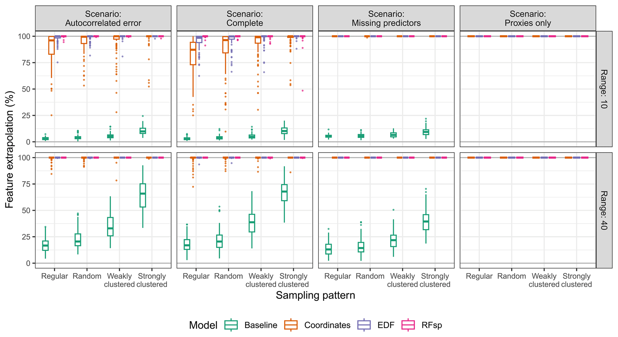
Figure A2 Feature extrapolation expressed as the percentage of the extrapolation prediction area outside of the area of applicability (AOA) of each model type, based on the prediction scenario, spatial-autocorrelation range, and sampling pattern.

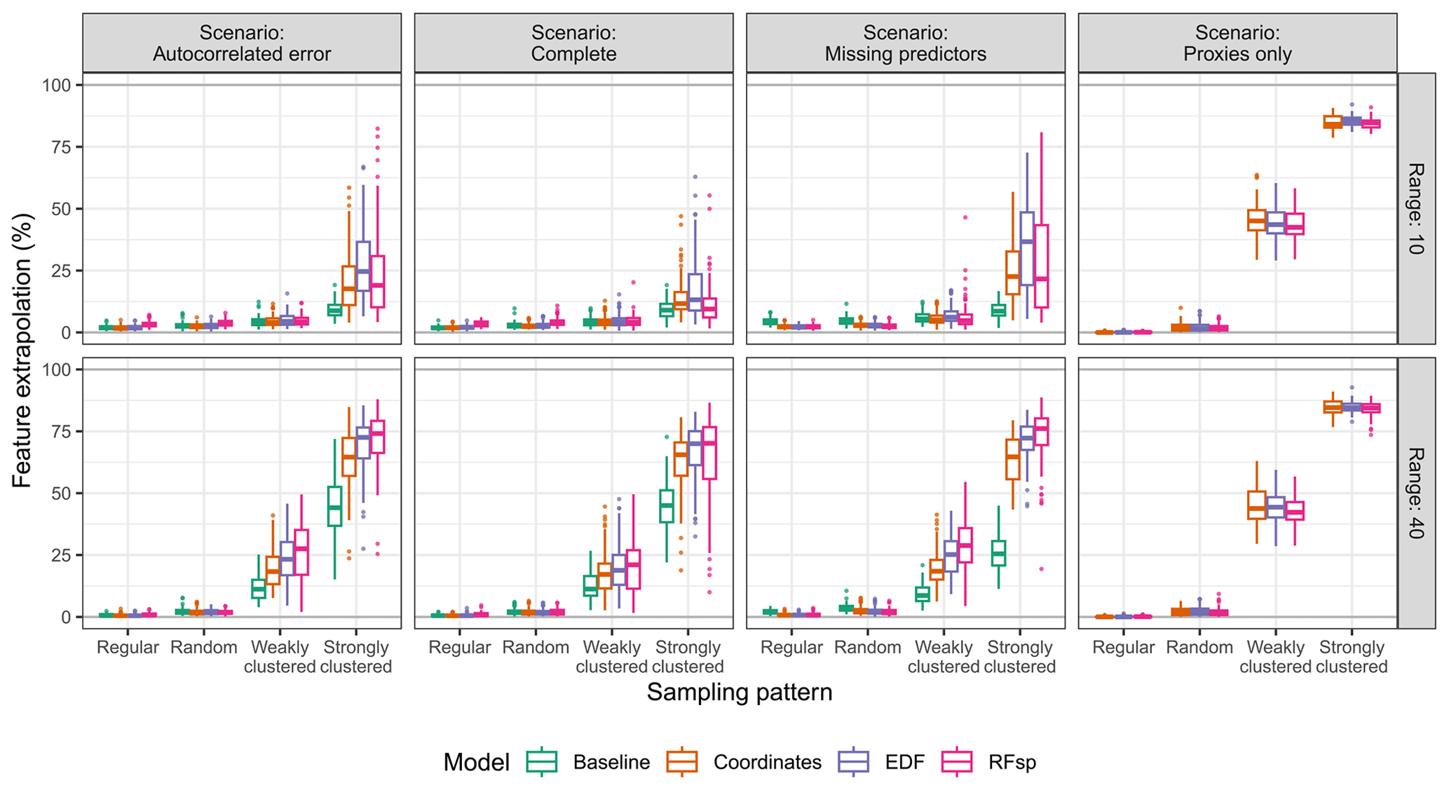
Figure A3 Feature extrapolation expressed as the percentage of the interpolation prediction area outside of the area of applicability (AOA) of each model type, based on the prediction scenario, spatial-autocorrelation range, and sampling pattern.

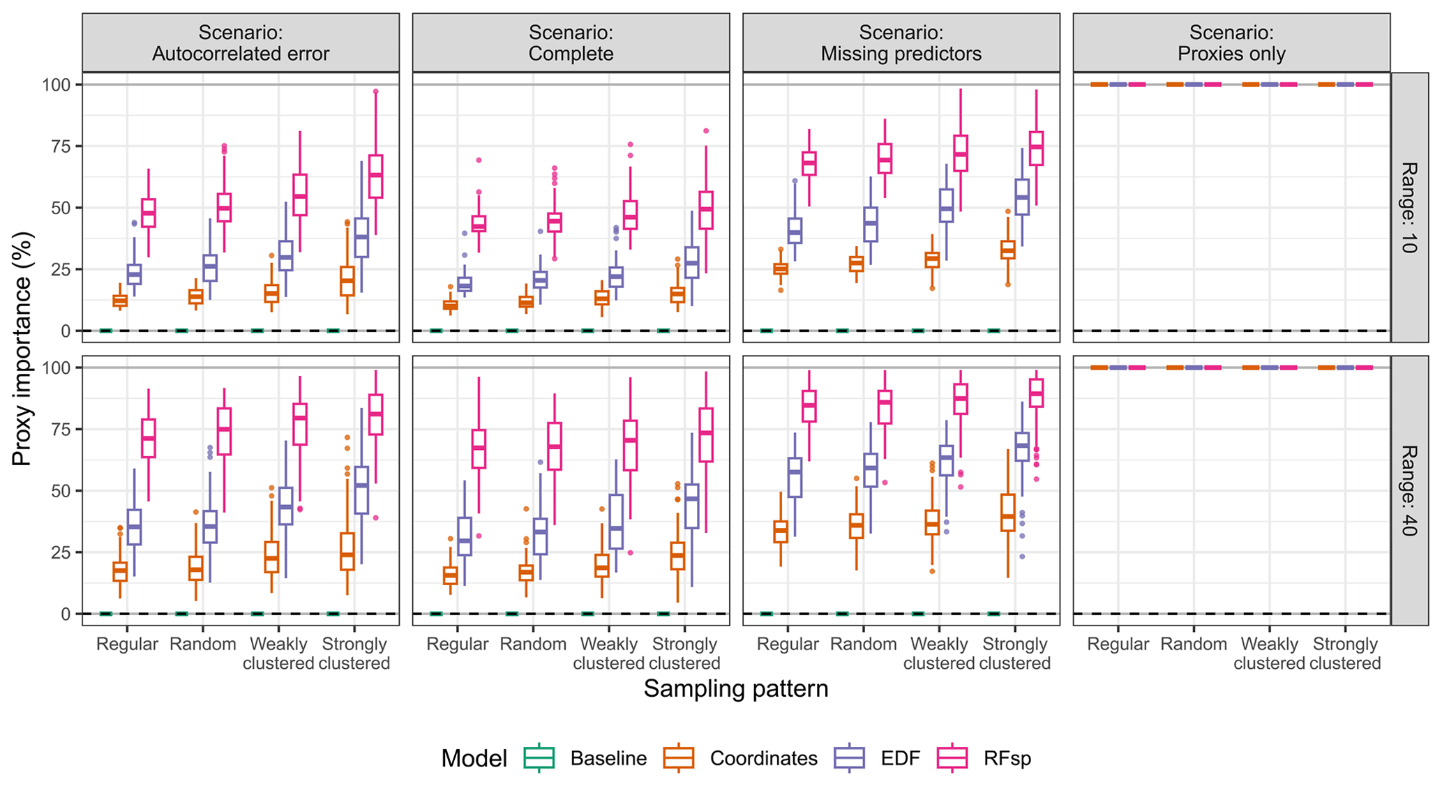
Figure A4 Variable importance of spatial proxies expressed as the percentage of the total mean impurity decrease attributable to the variables for each model type, based on the prediction scenario, spatial-autocorrelation range, and sampling pattern.

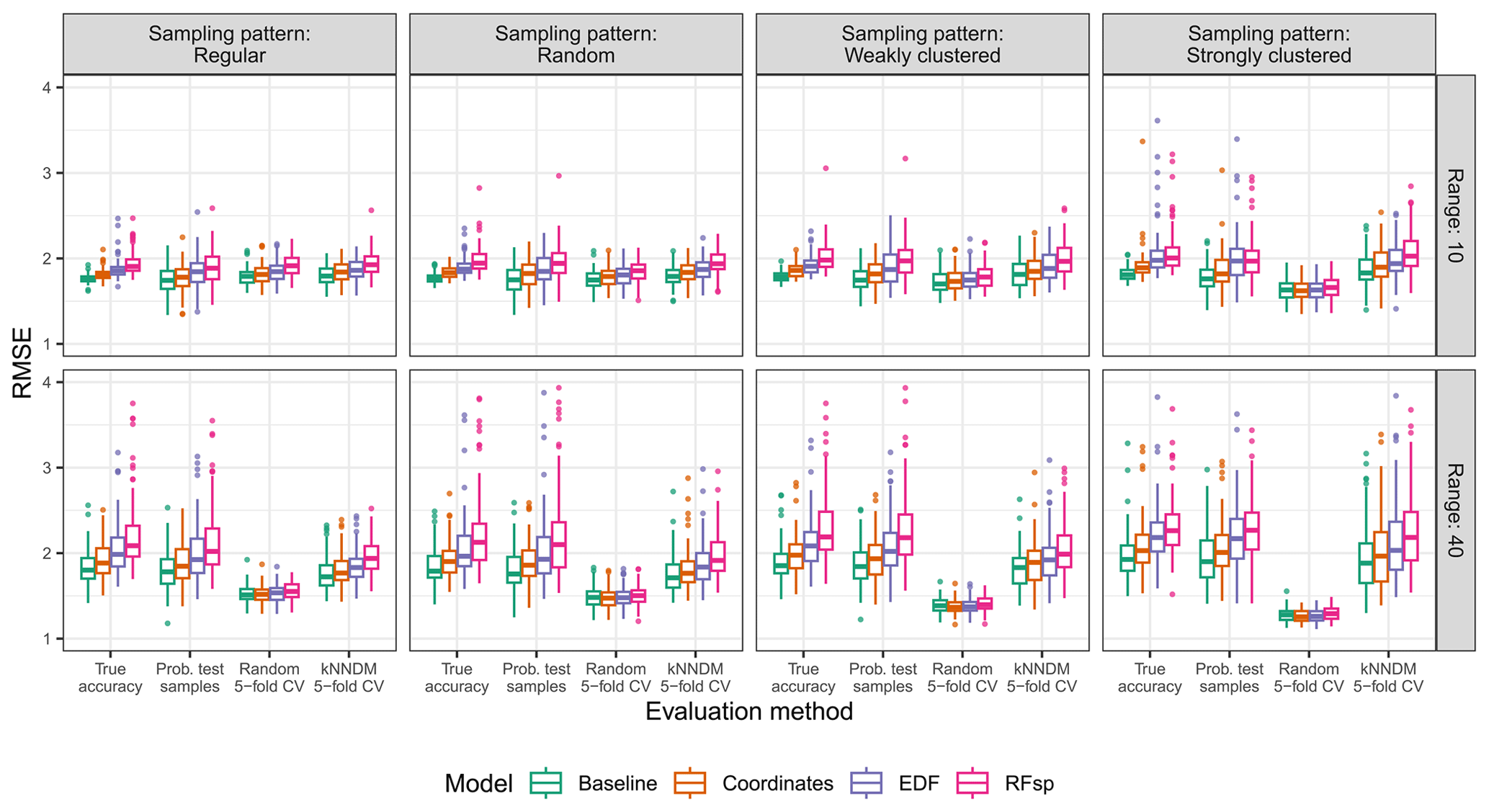
Figure A5 True and estimated RMSEs in the extrapolation area and the “complete” scenario, based on the evaluation method, autocorrelation range, and sampling pattern. Outliers larger than 4 are not shown for visualization purposes.

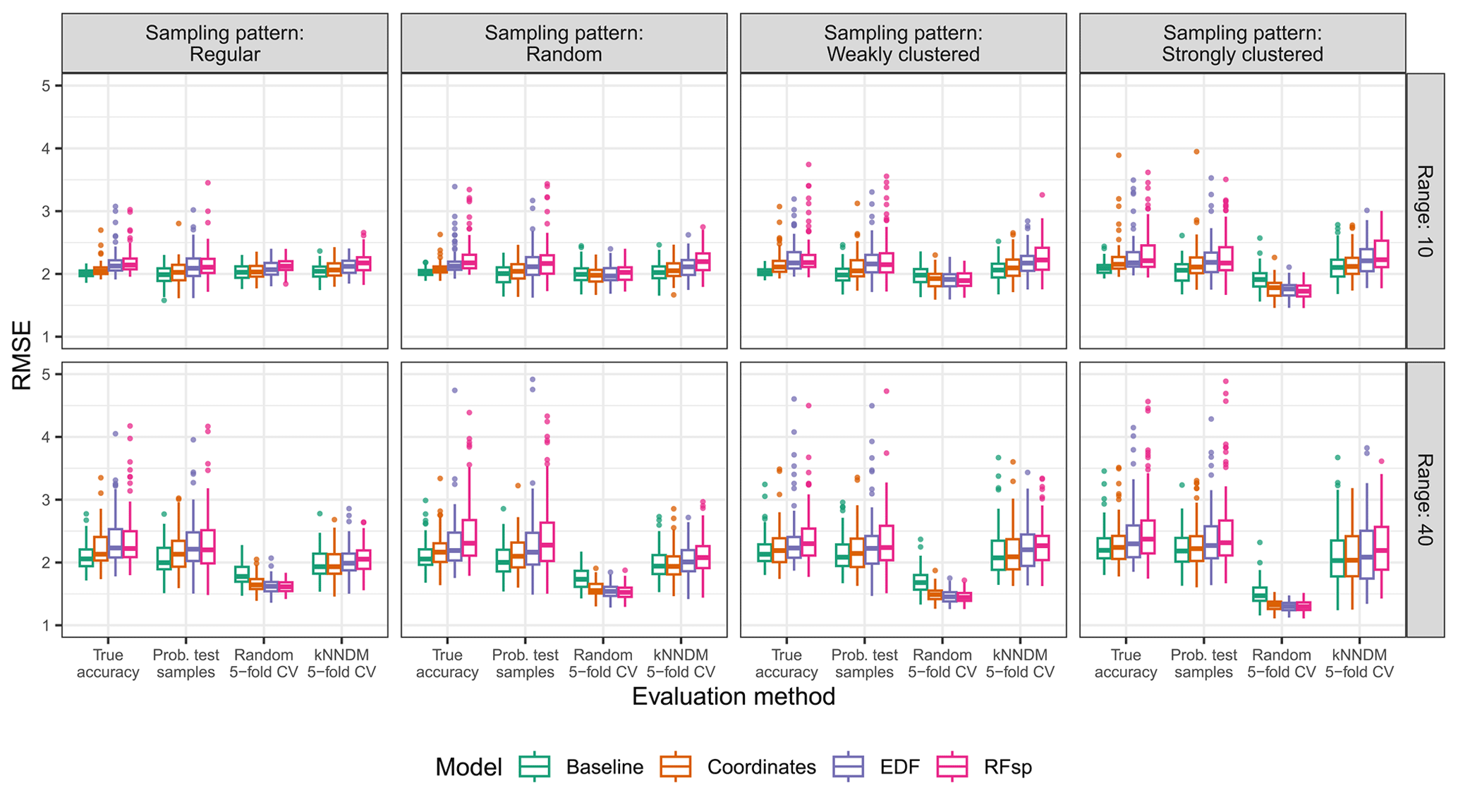
Figure A6 True and estimated RMSEs in the extrapolation area and the “missing predictors” scenario, based on the evaluation method, autocorrelation range, and sampling pattern. Outliers larger than 5 are not shown for visualization purposes.

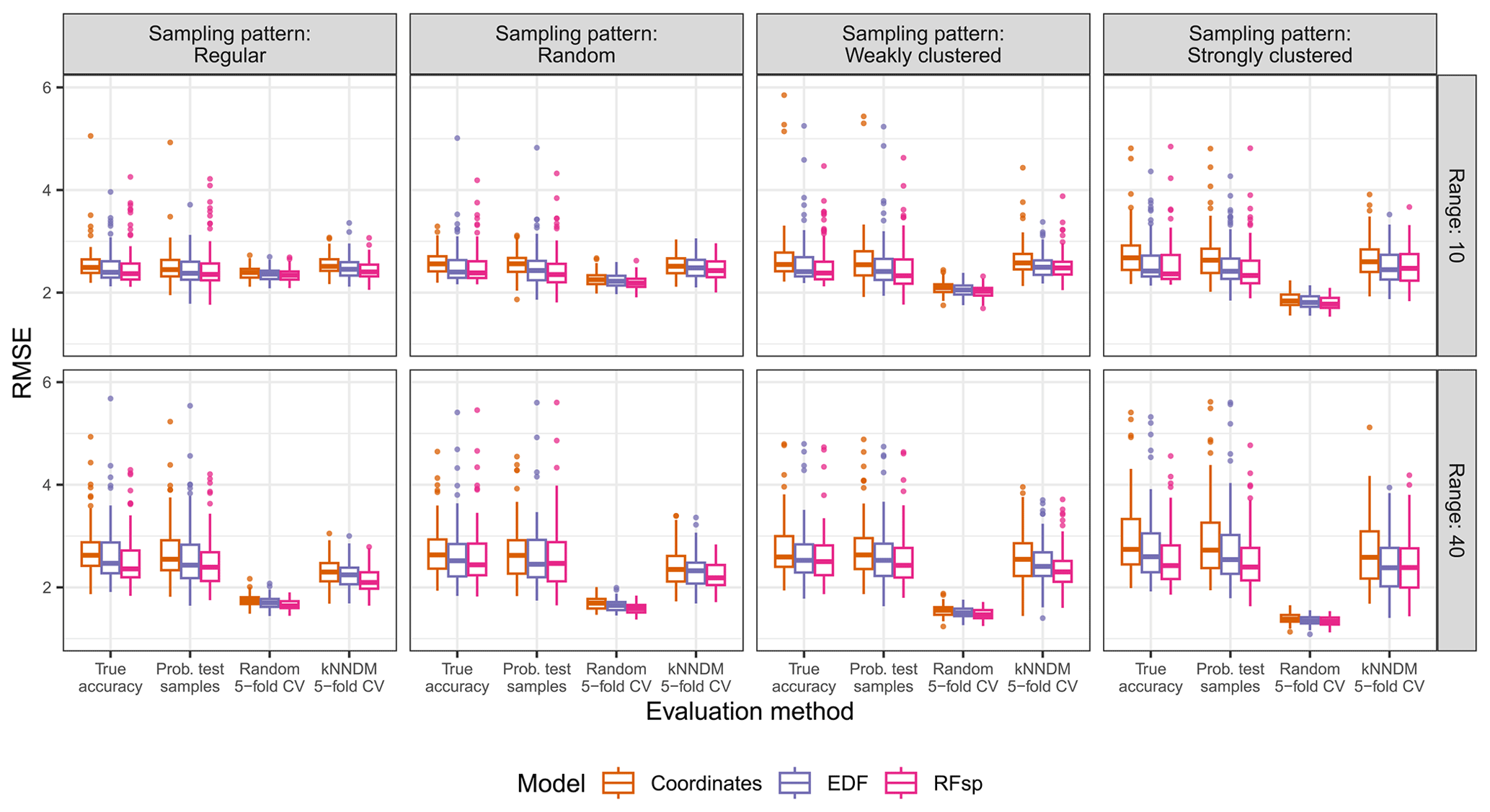
Figure A7 True and estimated RMSEs in the extrapolation area and the “proxies only” scenario, based on the evaluation method, autocorrelation range, and sampling pattern. Results for the baseline model were not calculated as no predictors were available for modelling. Outliers larger than 6 are not shown for visualization purposes.

Figure A8 True and estimated RMSEs in the interpolation area and the “complete” scenario, based on the evaluation method, autocorrelation range, and sampling pattern. Outliers larger than 3 are not shown for visualization purposes.

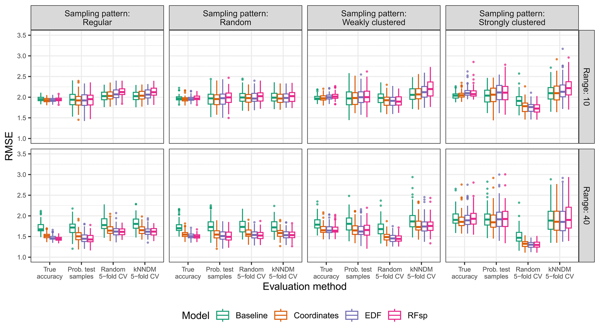
Figure A9 True and estimated RMSEs in the interpolation area and the “missing predictors” scenario, based on the evaluation method, autocorrelation range, and sampling pattern. Outliers larger than 3.5 are not shown for visualization purposes.

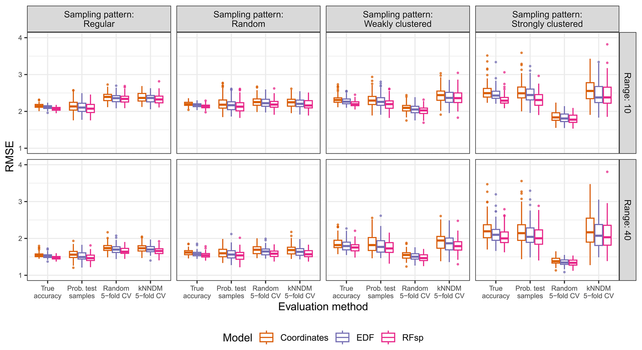
Figure A10 True and estimated RMSEs in the interpolation area and the “proxies only” scenario, based on the evaluation method, autocorrelation range, and sampling pattern. Results for the baseline model were not calculated as no predictors were available for modelling. Outliers larger than 4 are not shown for visualization purposes.

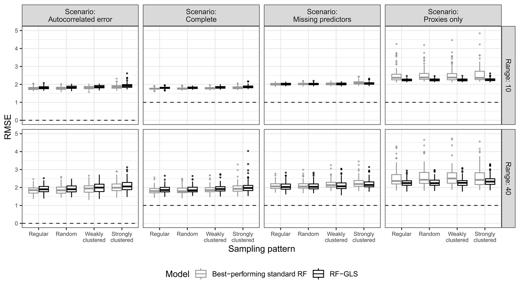
Figure A11 True RMSE in the extrapolation area of the best-performing standard RF for each simulation parameter combination (i.e. the standard RF model with/without proxies that has the lowest median RMSE) and the RF–GLS model, based on the prediction scenario, spatial-autocorrelation range, and sampling pattern.

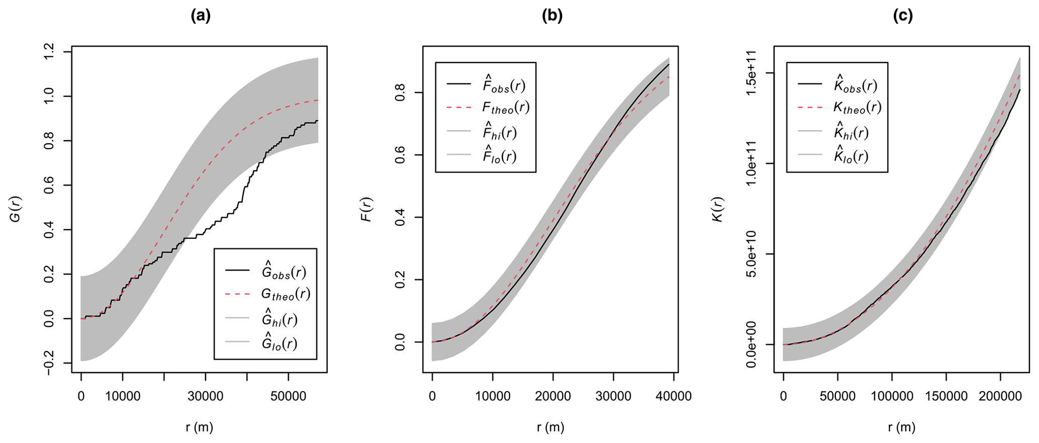
Figure A12 Empirical nearest neighbour distance distribution $\widehat{G}$ function (a), empty space $\widehat{F}$ function (b), and Ripley's $\widehat{K}$ pairwise distance function (c) for the air temperature case study. The dashed red lines indicate the theoretical function under complete spatial randomness (i.e. a homogeneous Poisson process), with its global envelope computed using 99 Monte Carlo simulations (shown in grey). Empirical functions calculated from the data are shown in black.

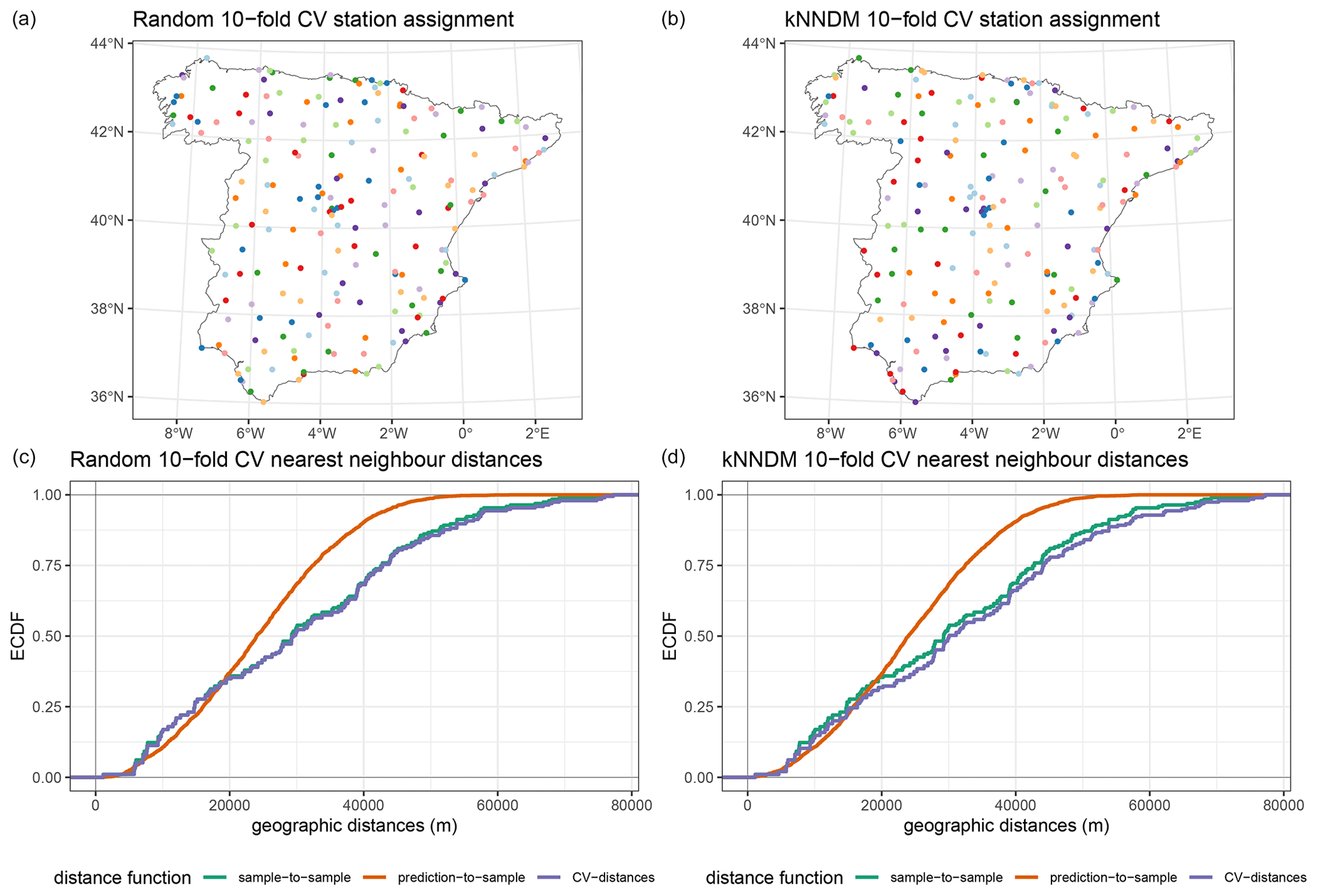
Figure A13 Fold assignment based on a 10-fold random CV method (a) and the kNNDM CV method (b) for the air temperature case study. Panels in the bottom row (c, d) display the corresponding empirical cumulative distribution functions (ECDFs) of the geographical sample-to-sample, prediction-to-sample, and CV nearest neighbour distances. Ideally, CV distances should match prediction-to-sample ECDFs as much as possible.

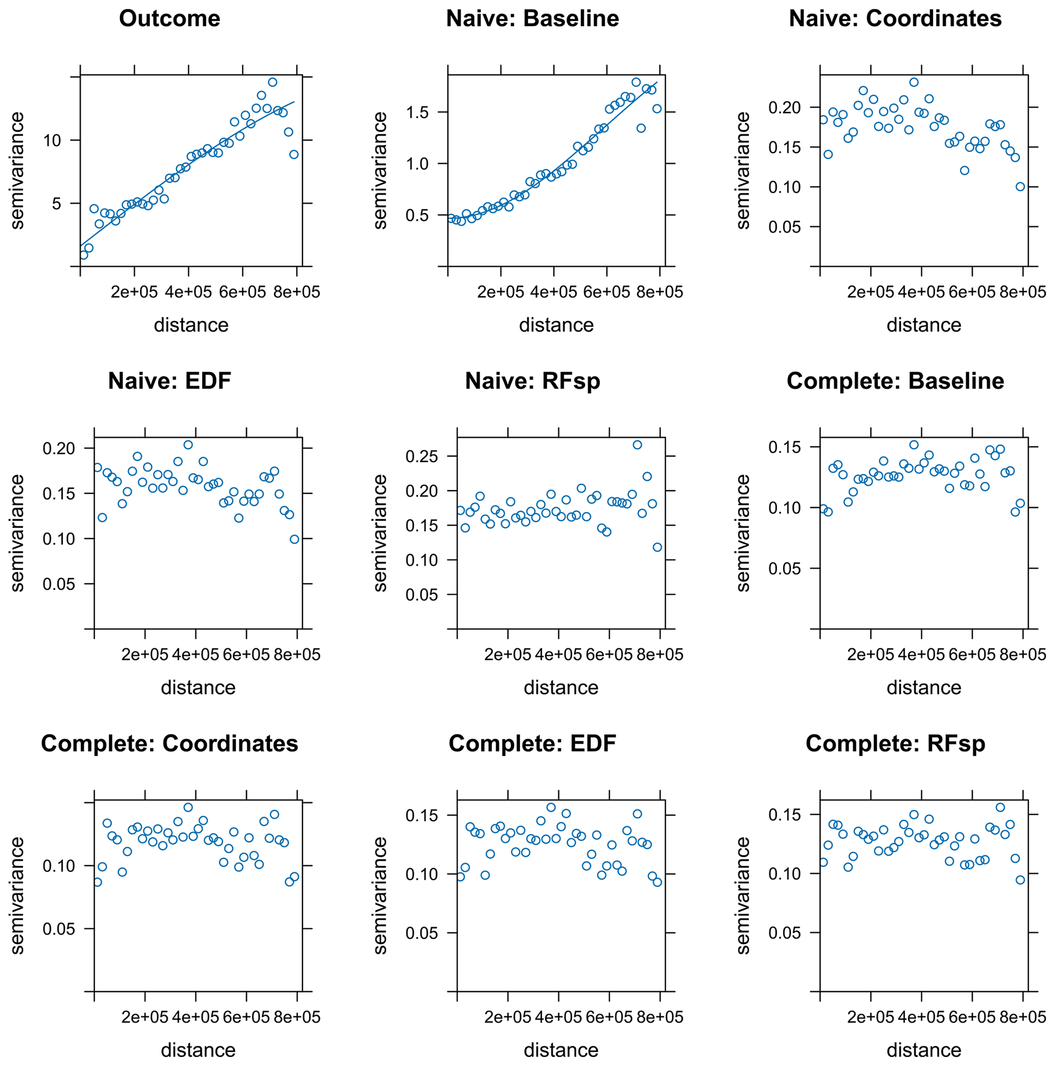
Figure A14 Empirical variograms for the air temperature response and residuals from all temperature models. Variogram models were fitted for illustrative purposes unless the fit did not converge.

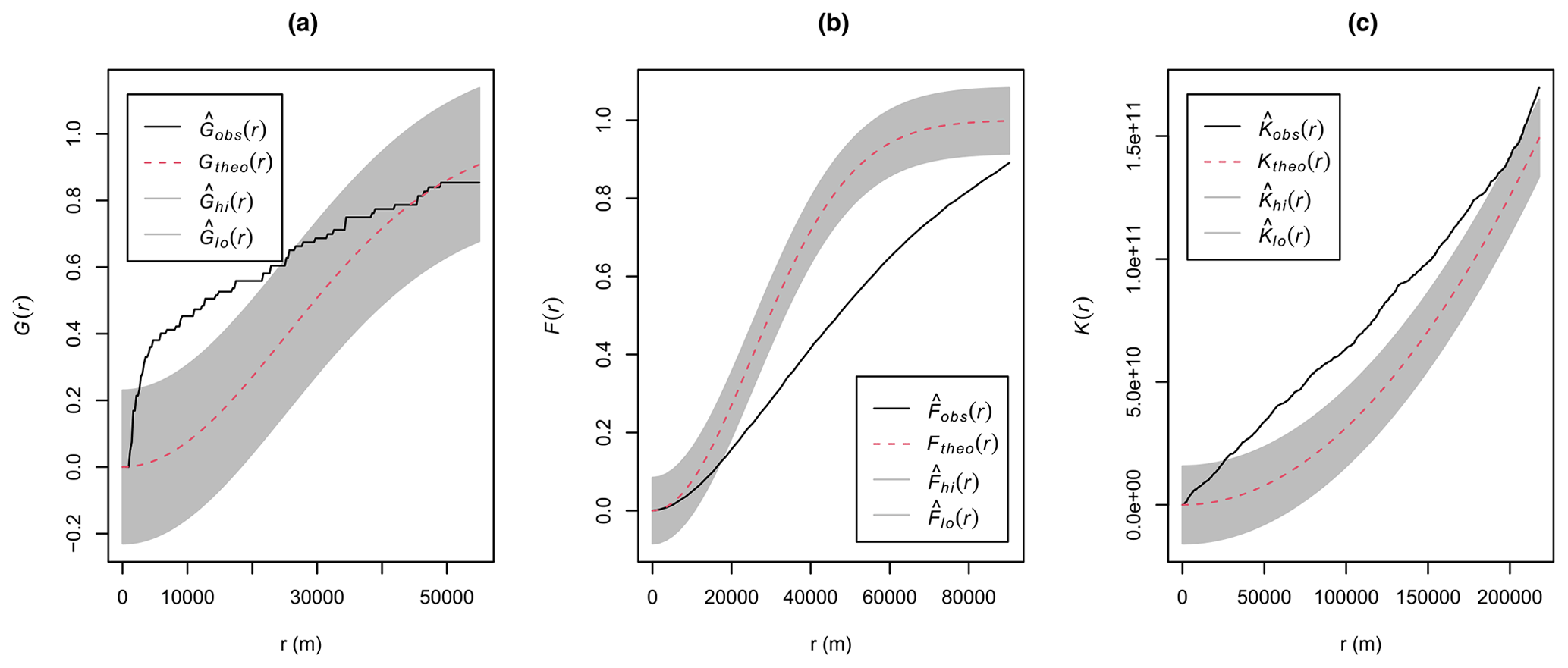
Figure A15 Empirical nearest neighbour distance distribution $\widehat{G}$ function (a), empty space $\widehat{F}$ function (b), and Ripley's $\widehat{K}$ pairwise distance function (c) for the PM_2.5 case study. The dashed red lines indicate the theoretical function under complete spatial randomness (i.e. a homogeneous Poisson process), with its global envelope computed using 99 Monte Carlo simulations (shown in grey). Empirical functions calculated from the data are shown in black.

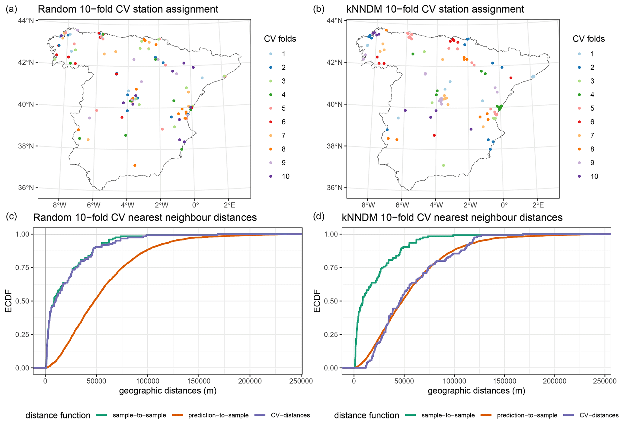
Figure A16 Fold assignment based on a 10-fold random CV method (a) and the kNNDM CV method (b) for the PM_2.5 case study. Panels in the bottom row (c, d) display the corresponding empirical cumulative distribution functions (ECDFs) of the geographical sample-to-sample, prediction-to-sample, and CV nearest neighbour distances. Ideally, CV distances should match prediction-to-sample ECDFs as much as possible.

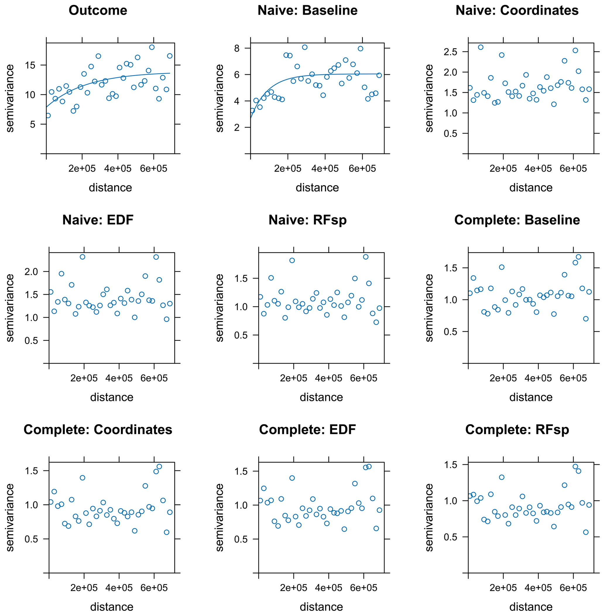
Figure A17 Empirical variograms for the PM_2.5 response and residuals from all PM_2.5 models. Variogram models were fitted for illustrative purposes unless the fit did not converge.

Table A1 List of products and their data sources, original spatiotemporal resolutions, and uses in the complete temperature and PM_2.5 models.

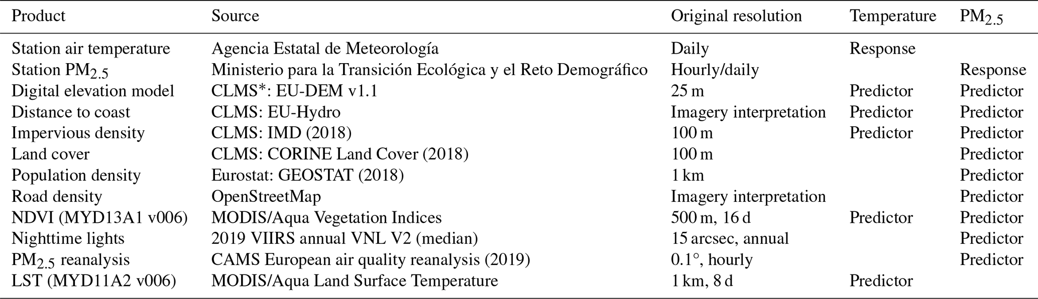
^* Copernicus Land Monitoring Service.