the Creative Commons Attribution 4.0 License.
the Creative Commons Attribution 4.0 License.
 | 25 Jan 2024
Sensitivity of air quality model responses to emission changes: comparison of results based on four EU inventories through FAIRMODE benchmarking methodology
Alexander de Meij
Cornelis Cuvelier
Philippe Thunis
Enrico Pisoni
Bertrand Bessagnet
Despite the application of an increasingly strict EU air quality legislation, air quality remains problematic in large parts of Europe. To support the abatement of these remaining problems, a better understanding of the potential impacts of emission abatement measures on air quality is required, and air chemistry transport models (CTMs) are the main instrument to perform emission reduction scenarios. In this study, we study the robustness of the model responses to emission reductions when emission input is changed. We investigate how inconsistencies in emissions impact the modelling responses in the case of emission reduction scenarios. Based on EMEP simulations over Europe fed by four emission inventories – EDGAR 5.0, EMEP-GNFR, CAMS 2.2.1 and CAMS version 4.2 (including condensables) – we reduce anthropogenic emissions in six cities (Brussels, Madrid, Rome, Bucharest, Berlin and Stockholm) and two regions (Po Valley in Italy and Malopolska in Poland) and study the variability in the concentration reductions obtained with these four emission inventories.
Our study reveals that the impact of reducing aerosol precursors on PM10 concentrations result in different potentials and potencies, differences that are mainly explained by differences in emission quantities, differences in their spatial distributions as well as in their sector allocation. In general, the variability among models is larger for concentration changes (potentials) than for absolute concentrations. Similar total precursor emissions can, however, hide large variations in sectorial allocation that can lead to large impacts on potency given their different vertical distribution. Primary particulate matter (PPM) appears to be the precursor leading to the major differences in terms of potentials. From an emission inventory viewpoint, this work indicates that the most efficient actions to improve the robustness of the modelling responses to emission changes would be to better assess the sectorial share and total quantities of PPM emissions. From a modelling point of view, NOx responses are the more challenging and require caution because of their non-linearity. For O3, we find that the relationship between emission reduction and O3 concentration change shows the largest non-linearity for NOx (concentration increase) and a quasi-linear behaviour for volatile organic compounds (concentration decrease).
We also emphasise the importance of accurate ratios of emitted precursors since these lead to changes in chemical regimes, directly affecting the responses of O3 or PM10 concentrations to emission reductions.
- Article
(1943 KB) - Full-text XML
-
Supplement
(3835 KB) - BibTeX
- EndNote


Despite the application of an increasingly strict EU air quality legislation, air quality remains problematic in large parts of Europe (EEA, 2020). This becomes even more crucial now that more stringent recent WHO guideline values (WHO, 2021) as well as the recently proposed EU limit values (EC, 2022) have acknowledged that air pollution can have negative impacts on health at much lower concentration levels for air pollutants such a PM10, PM2.5 and NOx. To comply with these higher-ambition limit values, a better understanding of the potential impacts of emission abatement measures on air quality is required. Air chemistry transport models (CTMs) are the main instrument to perform emission reduction scenarios, helping scientists and policymakers to understand which and how much of the emissions should be reduced to improve air quality. Over the years, CTMs continuously evolved by implementing more exhaustive and detailed chemical and dynamical atmospheric processes, and higher spatial grid resolution, to capture fine-scale features driven by land surface characteristics (De Meij et al., 2015, 2018).
Many studies exist that analyse the sensitivity of baseline concentrations to emissions or have compared model responses among themselves (Thunis et al., 2007, 2010, 2021a; Pernigotti et al., 2013 Vautard et al., 2007; Mircea et al., 2019). To the knowledge of the authors, very few works have assessed the sensitivity of model responses to the emission input (e.g. De Meij et al. (2009a); Aman et al. (2011); Miranda et al. (2015 and references therein). Other studies have investigated the uncertainties associated with certain processes when air chemistry models are used to support policymaking, such as meteorological input (De Meij et al., 2009a and references therein), aerosol chemistry (Thunis et al., 2021a; Clappier et al., 2021), model resolution (De Meij et al., 2007) or the emissions (Thunis et al., 2021b and references therein). Many of these topics are addressed in the framework of the Forum for Air Quality Modelling (FAIRMODE) (https://fairmode.jrc.ec.europa.eu/home/index; last access: 19 January 2024) that provides air quality modellers with a permanent forum to address air quality modelling issues. One of FAIRMODE's goals is also to assess the sensitivity of model responses to emission reductions in general. In this study, the robustness of the model responses to emission reductions is assessed when the emission input data are changed. While in Thunis et al. (2022), the authors compared emission inventories among themselves and proposed an approach to identify inconsistencies, here we investigate how these inconsistencies impact the modelling responses in the case of emission reduction scenarios. It is indeed crucial to better assess the share of the uncertainty that is associated with emission inventories in the overall uncertainty of the modelling response (Georgiou et al., 2020) as this is a key model output when designing air quality plans.
In light of the above, we investigate in this work the robustness of model responses to emission changes with a CTM based on four emission inventories and use specific indicators for the analysis. To this end, we perform simulations over Europe with the air chemistry transport model EMEP (Simpson et al., 2012), fed by the EDGAR 5.0, EMEP-GNFR, CAMS version 2.2.1 and CAMS version 4.2 + condensables emission inventories. We reduce anthropogenic emissions in six cities (Brussels, Madrid, Rome, Bucharest, Berlin and Stockholm) and two regions (Po Valley in Italy and Malopolska in Poland) and study the variability in the concentration reductions obtained with these four emission inventories feeding the EMEP model, considering a meteorology fixed at 2015. More details on the model, methodology and emission inventories are given in Sect. 2. We discuss the results in Sect. 3 and we conclude in Sect. 4.
Four emission inventories are used to feed the EMEP model to understand how this input data influences the calculated model changes in air pollutant concentrations. We performed one BaseCase (no emission reduction) simulation with each emission inventory for the year 2015 over Europe.
For the scenarios, we reduced for each emission inventory the emissions of NOx, volatile organic compounds (VOCs), NH3, SOx and primary particulate matter (PPM) which includes both their fine (size <2.5 µm) and coarse (2.5 µm < size <10 µm) by 25 % and 50 % for each species separately. This is done for six cities (Brussels, Madrid, Rome, Bucharest, Berlin and Stockholm) and two regions (Malopolska in Poland and Po Valley in Italy) to study the impact on particulate matter (PM) and ozone (O3) formation. (More details on the model and the emission inventories are given in the next section.) Because emissions are reduced in all cities and regions in a single simulation, these cities and regions must be far away from each other to avoid that emission reductions applied in one location influence background concentration levels in others. This constraint limits the number of cities and regions that we can cover in this work.
These emission reductions are theoretical and do not link with specific measures. For Malopolska and Po Valley the emissions are reduced over the whole modelling domain, as described in Table S1 in the Supplement. However, we analyse the impact of the emission reductions only over the city centres of Krakow and Milan, respectively. An overview of the characteristics of each modelling domain and the area over which the emissions are reduced is provided in Table S1. Below we present the air quality model and the emission inventories used in this study, together with the relevant indicators considered for this study.
2.1 The EMEP air quality model
In this study the EMEP model version rv_34 is used, which is an off-line regional transport chemistry model (Simpson et al., 2012; https://github.com/metno/emep-ctm; last access: 19 January 2024), to study the sensitivity of model responses to emission changes.
The model domain stretches from −15.05∘ W to 36.95∘ E longitude and 30.05 to 71.45∘ N latitude with a horizontal resolution of and 20 vertical levels, with the first level around 45 m. The EMEP model uses meteorological initial conditions and lateral boundary conditions from the European Centre for Medium Range Weather Forecasting (ECMWF-IFS) for the meteorological year 2015. The temporal resolution of the meteorological input data is daily, with 3 h time steps. The initial and background concentrations for ozone are based on Logan (1998) climatology, as described in Simpson et al. (2003). For the other species, background/initial conditions are set within the model using functions based on observations (Simpson et al., 2003; Fagerli et al., 2004). Secondary aerosol formation (Simpson et al., 2012) accounts for complex chemical and physical processes, such as sulfate aerosol formation from SO2, nitrate aerosol formation from NOx or organic aerosol formation from VOCs. (More detailed information on the meteorological driver, land cover, model physics and chemistry is provided in De Meij et al. (2022) and references therein.)
2.2 Emission inventories
In this study we used the anthropogenic emissions of four emission inventories, all for the year 2015. The emission inventories are:
-
EDGAR v5.0
-
EMEP-GNFR
-
CAMS-REG v2.2.1
-
CAMS-REG v4.2 with condensables.
Note that, while EDGAR is completely independent from the other emission inventories, there are common features in the other three inventories. For example, emission inventories 2 and 3 share the same country totals but use different proxies to spatialise emissions; while emission inventories 3 and 4 differ in terms of release date and emission updates from 2.2.1 to 4.2 with 4 also containing condensables in addition to 3. “Condensables” represent the fraction consisting of organic vapour able to react and/or produce condensed species when cooling.
Table 1Overview of the four emission inventories used in this study.

* Total emissions (in kt yr−1) for Austria, Belgium, Bulgaria, Denmark, Finland, France, Greece, Hungary, Ireland, Italy, Luxembourg, the Netherlands, Poland, Portugal, Romania, Spain, Sweden, Estonia, Latvia, Lithuania, Czech Republic, Slovakia, Slovenia ,Croatia, Cyprus, Malta and Germany.
All emissions are detailed in terms of the GNFR classification (Table S2), where GNFR stands for Gridded Nomenclature for Report. An overview of the characteristics of the emissions inventories is given in Table 1. The anthropogenic emissions in the four inventories are CO, NOx, SOx, NH3, VOC, PM2.5 and PM10.
2.2.1 EDGAR
The Emissions Database for Global Atmospheric Research (EDGAR) is a global inventory providing greenhouse gas and air pollutant emissions estimates for all countries over the time period 1970 till most recent years, covering all IPCC reporting categories with the exception of Land Use, Land Use Change and Forestry (LULUCF). It uses a bottom-up approach, i.e. using activity data and country specific emission factors based on IPCC recommendations to estimate emission quantities (Crippa et al., 2018).
For this work, we use the EDGAR 5.0 inventory (hereafter “EDGAR”), which contains anthropogenic emissions for aerosol and aerosol precursor gases at 0.1×0.1 horizontal resolution. The inventory is available at https://EDGAR.jrc.ec.europa.eu/dataset_ap50; last access: 19 January 2024; Janssens-Maenhout et al., 2019; Crippa et al., 2020). (More information about the emission inventory is given in Thunis et al. (2021b) and references therein.)
2.2.2 EMEP-GNFR
The EMEP emissions (Mareckova et al., 2018), further denoted as EMEP-GNFR, are compiled within the “UNECE co-operative programme for monitoring and evaluation of the long-range transmission of air pollutants in Europe” (unofficially “European Monitoring and Evaluation Programme” (EMEP)). The EMEP is a scientifically based and policy-driven programme under the Convention on Long-Range Transboundary Air Pollution (CLRTAP) for international co-operation, which has the final aim of solving transboundary air pollution problems. More specifically, the EMEP emissions are built from officially reported data provided to the Centre of Emission Inventory and Projection (CEIP), a body of EMEP, by the Convention parties. Emissions are gap-filled with gridded TNO data from Copernicus Atmospheric Monitoring Service (CAMS) and EDGAR. The dataset consists of gridded emissions for SOx, NOx, NMVOC, NH3, CO, PM2.5, PM10 and PMcoarse at resolution. (More information on the emissions and where to download the relevant information can be found in the user guide (https://emep-ctm.readthedocs.io/_/downloads/en/latest/pdf/, last access: 19 January 2024 and in Mareckova et al., 2018)
2.2.3 CAMS-REG v2.2.1
The Copernicus Atmosphere Monitoring Service Regional Anthropogenic Air Pollutants (CAMS-REG-AP) emission inventory (Granier et al., 2019) covers emissions for the UNECE-Europe for CH4, NMVOC, CO, SO2, NOx, NH3, PM10, PM2.5 and CO2 and CH4. Version 2.2 (hereafter “CAMS221”) and newer is an update of the TNO_MACC, TNO_MACC-II and TNO_MACC-III inventories (Kuenen et al., 2014, 2021).
The CAMS-REG-AP methodology starts from the emissions reported by European countries to UNFCCC (for greenhouse gases) and to EMEP/CEIP (for air pollutants), aggregated into different combinations of sectors and fuels. Then, these emissions are gridded using ad-hoc proxies, which differ from the ones used in EMEP-GNFR. The spatial resolution of the emissions is . (More information can be found in Granier et al., 2019 and Thunis et al., 2021b.)
2.2.4 CAMS-REG v4.2 + condensables
This inventory (Kuenen et al., 2021, 2022) is an update of the previous CAMS versions for PM emissions for the residential sector, also known as REF1, in which PM2.5 and PM10 emissions have been updated with information on the condensable part (TNO, 2021; Jeroen Kuenen, personal communication). This inventory, also known as REF2, is hereafter referred to as “CAMS42C”. Condensables replace country reported PM2.5 and PM10, with a bottom-up estimate for small combustion for all fuels (not only wood but also fossil fuels). Since 2016, more and more countries have gradually included condensable emissions of small combustion devices, leading to significant differences as shown by Kuenen et al. (2022). For example, in countries such as Poland and Turkey where coal combustion in households is still an important contributor to PM, large emissions of fine and coarse condensables (118 kT yr−1 for PM2.5) still take place. For Turkey the difference in PM2.5 emissions for GNFR Sector 03 is around 20 % (higher in CAMS42C). For Hungary, Slovakia, Ireland, UK, Belgium and Norway the PM2.5 emissions for GNFR Sector 03 are in general lower than in CAMS42C.
Edgar uses a bottom-up approach for all emission source sectors, based on estimates of activity data and emission factors, whereas CAMS is mainly based on countries' reported emissions. The differences between the same years between the CAMS inventories stems from the recalculations of the pollutants for each country.
More in-depth analysis and explanations on the underlying differences between the emission inventories, as used in this study, is given in Thunis et al. (2022). They identify the largest inconsistencies between the emission inventories in terms of pollutant and sector for 150 cities in Europe and show that the difference for some air pollutants between emission inventories can be as large as a factor of 100 or more. They explain that the underlying reason for these discrepancies is related to the differences in spatial proxies, country totals (i.e. differences in urban area share) and country sectoral share (e.g. industry, residential and power plants).
2.3 Indicators for the comparison
In this section we analyse the impact of the emission reduction on simulated yearly change of concentrations for the six cities and two regions. To perform this analysis, we use the potency and potential indicators as defined in Thunis et al. (2015a, b) based on 50 % emission reduction strengths. These indicators are specifically designed to analyse the impact of emission reductions on concentration changes. We only recall their basic definitions here:
The absolute potential (AP) is defined as the concentration change (between the BaseCase and the scenario) divided by the reduction strength. It is expressed in µg m−3:
where CBaseCase represents the BaseCase yearly concentrations, obtained with one of the four emission inventories (no emission reduction); Cscenario the “scenario” yearly concentrations; and alpha the emission reduction strength, i.e. alpha =0.25 (25 % reduction) and alpha =0.50 (50 % reduction). All indicators are calculated as 95th percentiles, i.e. based on the average of all BaseCase concentration values modelled in a given area that exceeds the 95th percentile concentration threshold. Note that the grid cells for these concentration values are selected from the BaseCase obtained with a given inventory. They are kept unchanged for the scenario but can differ from one emission inventory to the other. The absolute potential informs the concentration change projected linearly to 100 % from a given scenario.
The relative potential (RP) is obtained by dividing the absolute potential by the BaseCase concentration:
The RP provides similar information to the AP, but because it normalises the concentration change by the BaseCase concentration, it removes the impact of potential biases among BaseCases when different models (here intended as a single model fed by different emissions) are compared with each other.
The potency (P) in µg m−3/(t d−1) is defined as the ratio of the concentration change by the emission change E:
The potency informs the potential concentration change per unit emission change. The normalisation by the emission change allows us (at least partly) to exclude the impact of differences in the absolute levels of emissions in models when performing the comparison.
2.4 Screening method statistical analysis
In this section, we provide a summary of the screening method which is adapted from Thunis et al. (2022). The approach aims at comparing the modelling responses from different models over a series of geographical areas. Based on emissions detailed in terms of precursors (denoted as “p”) and city areas (denoted as “c”), the consistency between two modelled responses (or absolute potential – AP) is decomposed into two aspects: the potency (P) and the underlying emissions (E). To do this, we decompose the ratio of the known absolute potentials of two models for each city as follows:
Superscripts refer to the two models. Equation (1) is an identity where all terms are known from input quantities, i.e. the two modelled absolute potentials detailed in terms of precursors and cities on the left-hand side and the ratios of the potencies and emissions on the right-hand side. E is here intended as the absolute emission values. Multiplied by alpha, we then obtain the emission reduction change, i.e. delta E= alpha ×E.
For convenience, we rewrite Eq. (1) in logarithmic form (2), considering the absolute values of the potencies only, as
which can be rewritten as Eq. (3) with simplified notations:
where the hat symbol indicates that quantities are expressed as logarithmic ratios. These quantities are at the basis of the screening methodology and serve as inputs for the graphical representation as well. The implicit assumption is that AP1 and AP2 or P1 and P2 have the same sign. This is true in most cases, except in a case of strong non-linearities such as for ozone.
We proceed with a number of steps that help in focusing on priority aspects. First, we restrict the screening only to absolute potentials that are relevant, i.e. large enough. This is achieved by requiring that any given potential fulfil the following condition: to be further considered in the screening, where γ is a user defined threshold parameter, set to 20 % in this work. Second, we flag, among the remaining potentials, only those for which differences between models are larger than a threshold, β, also set to 20 % in this analysis. Beyond this threshold, differences are thought to be large enough to justify further checking. These thresholds are arbitrary but they should be set in such a way that significant model differences only are spotted while keeping the analysis reasonable (e.g. the number of identified inconsistencies). These thresholds can also be lowered with time if inconsistencies are progressively resolved or explained.
Equation (3) is the basis of the “diamond” shape (see Fig. 3 as an example) that provides an overview of all inconsistencies detected during the screening process. In these diagrams of Fig. 3, each inconsistent potential is represented by a point that has absolute total emissions () as abscissa and potency as ordinate (). The sum of these two terms () is equal for points that lie on “−1” slope diagonals. At this stage it is important to note that positive differences in terms of emissions and potencies will characterise points lying on the right and top parts of the diagrams in Fig. 3, respectively. In addition, the upper right and lower left diagram areas indicate summing-up effects, whereas the lower right and top left areas highlight compensating effects.
The diamond shape (in the middle of Fig. 3) derives from Eq. (3) where the β threshold is used to draw the inconsistency limit for each of its two terms, as well as their sum. Each pollutant/city (p,c) point lying outside this shape is therefore characterised by an inconsistency in terms of either E or P and/or AP, small or large according to its distance from the diamond.
In Fig. 3, shapes are used to differentiate precursors while colours differentiate cities. To reflect the differences in potentials (concentration change resulting from an emission reduction) of different precursors, the size of a symbol is set proportionally to the maximum potential found over all precursors and all models, for each city. Finally, we use symbol filling to distinguish cases where the modelled responses change signs (filled symbol) between models (i.e. a positive vs. a negative concentration change).
We also use the median concept as discussed in Thunis et al. (2023). The median is calculated from three emission inventories: EDGAR, CAMS221 and EMEP-GNFR. The proposed approach then consists of comparing each model (i.e. EMEP with one inventory) with the median to identify inconsistencies (see Thunis et al., 2023 for more details). The median is not meant here to represent a more accurate model response but rather as a common benchmark by which to compare models.
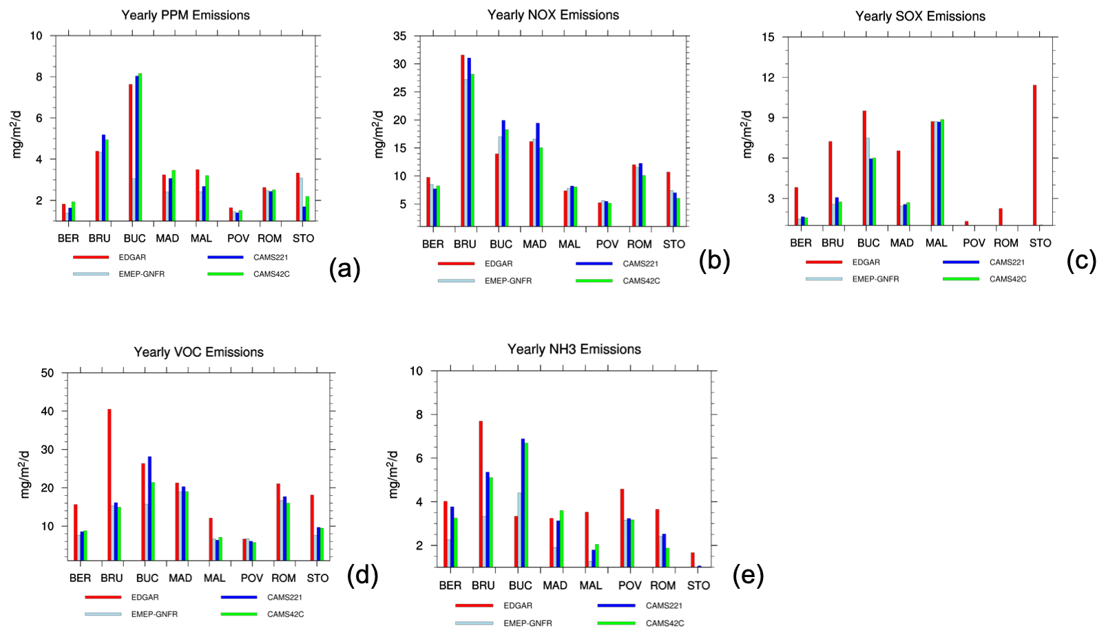
Figure 1Annual mean emission densities (in mg m2 d−1) for (a) PPM, (b) NOx, (c) SOx, (d) VOC and (e) NH3 by EDGAR (red), EMEP-GNFR (light blue), CAMS221 (blue) and CAMS42C (green) for the eight locations (Berlin (BER), Brussels (BRU), Bucharest (BUC), Madrid (MAD), Malopolska region (MAL), Po Valley region (POV), Rome (ROM) and Stockholm (STO)).
In this section we first assess the level of consistency in terms of input emissions, the driving factor for potential differences, before analysing their impact in terms of concentration changes.
3.1 Analysis of the emissions
Analysing the PPM emissions from the four emission inventories in Fig. 1, we see that all emissions compare well in general, apart from EMEP-GNFR in Bucharest (lower) and CAMS221 in Stockholm (lower). EDGAR (red coloured) registers the highest PPM emissions for Malopolska, Po Valley, Rome and Stockholm. The differences in PPM emissions between CAMS221 and CAMS42C can be explained by the replacement in the CAMS221 (REF1) inventory of country-reported PM2.5 and PM10 emissions for residential heating by emissions that account for condensables in CAMS42C. Condensables are emitted as gaseous compounds that immediately condense to form organic aerosols. They lead to overall higher PM emissions in CAMS42C. Significant changes in PM2.5 emission quantities due to the presence of condensables are found for several countries, like Spain, Italy and Romania, while differences are smaller for Germany and France (Kuenen et al., 2022). This corroborates the higher PPM emissions in CAMS42C than in CAMS221 for Po Valley, Rome, Madrid and Stockholm found in this study. The emission quantities for each location, pollutant and inventory are given in Table S3.
Furthermore, Kuenen et al. (2022) showed that the emission differences between CAMS221 and CAMS42C can be explained by the different methodologies and recalculation of the officially reported emissions. Also, each year, an update is processed of a given country's past reported emissions based on the latest information of activity data or emission factors (EFs). This helps to explain the differences between the emission inventories and reported years.
Kuenen et al. (2022) also showed that in general, for Europe, NMVOC, NH3, PPM10, PPM2.5, NOx and SO2 emissions are higher in EDGAR than in CAMS42, with larger differences for non-EU countries. This could be explained by the fact that EDGAR uses a bottom-up methodology instead of the reported country totals, which has been shown to have, in general, higher uncertainties (Cheewaphongphan et al., 2019).
In our study, we compare the emission densities for smaller areas, but we find similar differences, i.e. EDGAR registers higher emissions for the above-mentioned pollutants for the eight areas considered in our study, apart from yearly NOx emissions for Bucharest, Madrid, Malopolska, Rome and Po Valley, where the emission densities are similar to the other emission inventories. Also, there are substantial differences in PPM emissions for Bucharest between EMEP-GNFR (3.1 mg m2 d−1) and the other three inventories, 7.6 mg m2 d−1 for EDGAR, 8.0 mg m2 d−1 for CAMS221 and 8.2 mg m2 d−1 for CAMS42C, which clearly impact the model responses (in terms of concentration) to emission reductions, as will be further discussed in the next section.
Overall, SOx, NH3 and VOC by EMEP-GNFR and the two CAMS inventories agree well, while EDGAR generally shows higher emission densities for these pollutants except for Bucharest and Po Valley for VOC and NH3 for Madrid and Bucharest.
More details on the explanation regarding the differences between CAMS221, CAMS42C and EDGAR are described in Kuenen et al. (2022). At the urban scale, Thunis et al. (2021b) showed that for some sectors and pollutants, the EDGAR emissions were significantly larger than other inventories. This is the case for the SO2 emissions from the industrial sector because of differences in terms of country totals but also in terms of spatial proxies used.
3.2 Variability in PM10 BaseCase concentrations
Yearly averaged PM10 concentrations from EDGAR are in general higher than with the other emission inventories, except for Brussels, Madrid and Stockholm (Fig. 2). We have seen in Sect. 3.1 that for some locations PPM, SOx, NH3 or NMVOC emissions from EDGAR are higher than the other three inventories. However, differences in emissions do not lead to important differences in terms of PM10 concentrations.
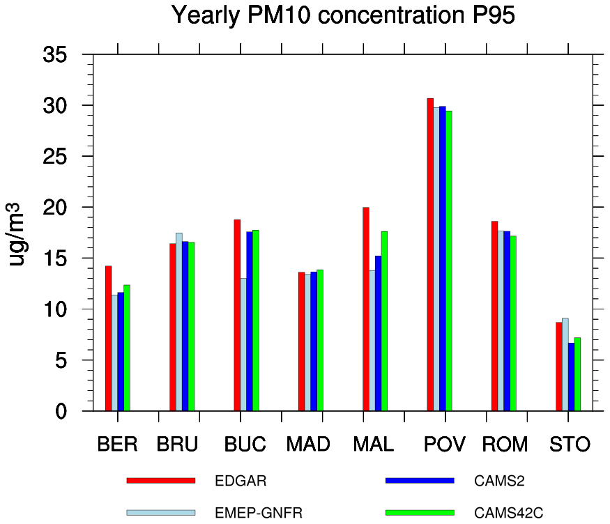
Figure 2Total yearly average PM10 concentrations by EDGAR (red), EMEP-GNFR (light blue), CAMS221 (blue) and CAMS42C (green) for the eight locations (Berlin (BER), Brussels (BRU), Bucharest (BUC), Madrid (MAD), Malopolska region (MAL), Po Valley region (POV), Rome (ROM) and Stockholm (STO)). The concentrations represent values above the 95th percentile values, showing the highest 5 % values in the domain from the BaseCase.
For Malopolska we find that PM10 values by CAMS42C are higher than CAMS221 and EMEP-GNFR due to the inclusion of condensables for residential heating. Note that inclusion of condensables leads to larger differences over Eastern Europe.
Interestingly, the large difference in PM10 concentrations for Bucharest between EMEP-GNFR and the other three inventories (EMEP-GNFR lower), which can be explained, at least partly, by the differences in PPM emissions, as mentioned in Sect. 3.1.
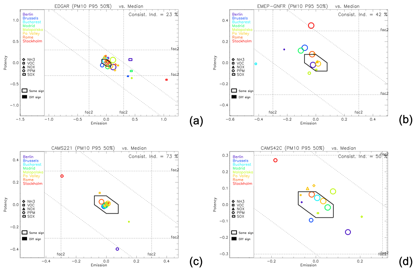
Figure 3Diamond plot for PM10 concentrations for (a) EDGAR, (b) EMEP-GNFR, (c) CAMS221 and (d) CAMS42C. The values represent values above the 95th percentile, showing the highest 5 % values in the domain from the BaseCase. The x and y axes are expressed as logarithms. For each city, the size of a symbol is proportional to the maximum absolute potential of the considered precursor, across models. Note that symbols for which emissions are relevant and that characterise the median all fall at the (0, 0) position. For visualisation purpose, these have been slightly shifted within the diamond shape.
3.3 Analysis of potentials and potencies for PM10
Figure 3 represents the impact on calculated PM10 concentrations of emission reduction in NH3, VOC, NOx, PPM and SOx for the different locations. The plots show the potency on the y axis, the emissions on the x axis and the potential (obtained at 50 %) along descending diagonal (indicated with dashed lines). The diamond shape indicates that differences in emissions, potencies and potentials between a given model and the median are below 20 %, where the median is calculated from three emission inventories: EDGAR, CAMS221 and EMEP-GNFR. The “fac2” lines indicate a factor of two difference as compared with the median, respectively. The consistency indicator (top right) provides information on the percentage of pollutant/city (p,c) couples that fall within the diamond shape, e.g. in the case of CAMS42C, 50 % of the (p,c) couples show differences with the median estimate that remain below 20 %. Below we analyse the results per precursor.
3.3.1 PPM
EMEP-GNFR calculates much higher potentials for PM10 in Stockholm, due to an overestimation of the PPM potency by a factor ∼2 (see Fig. 3b). For Bucharest a much lower potential for PM10 is found, which can be explained by the underestimation (around a factor 2) of the PPM emissions. Also, CAMS221 displays lower PPM emissions for Stockholm (Fig. 3c), but these lower emissions are compensated by higher potencies (factor ∼2 higher), leading to PM10 potentials similar to those of the other inventories. For Berlin, the CAMS221 PPM potency is more than a factor 2 lower, leading to underestimation in terms of potential of a factor ∼2, despite a slight overestimation of the emissions. Because PPM does not undergo chemical reactions, we expect a relatively linear relationship between emissions and concentrations. In other words, we expect emissions and potentials to be correlated (e.g. Bucharest for EMEP-GNFR). In some instances, this is, however, not the case (e.g. Stockholm for EMEP-GNFR and CAMS42C). These differences can partly be explained by the sector allocation of the PPM emissions in the four inventories, as shown in Fig. 4. EDGAR assigns much larger PPM emissions in sector 2 (industry), while EMEP-GNFR has larger PPM emissions in sector 6 (road transport). This is important as emissions are distributed vertically in a different way depending on the sector. Industrial emissions, mainly emitted by stacks at higher levels, travel over larger distances and will have less impact on surface concentrations locally than emissions emitted at ground such as road transport. This explains the much higher potencies in EMEP-GNFR for Stockholm. It also stresses the importance of the sectorial repartition of the emissions, especially for PPM which generally shows the largest potencies among all precursors.
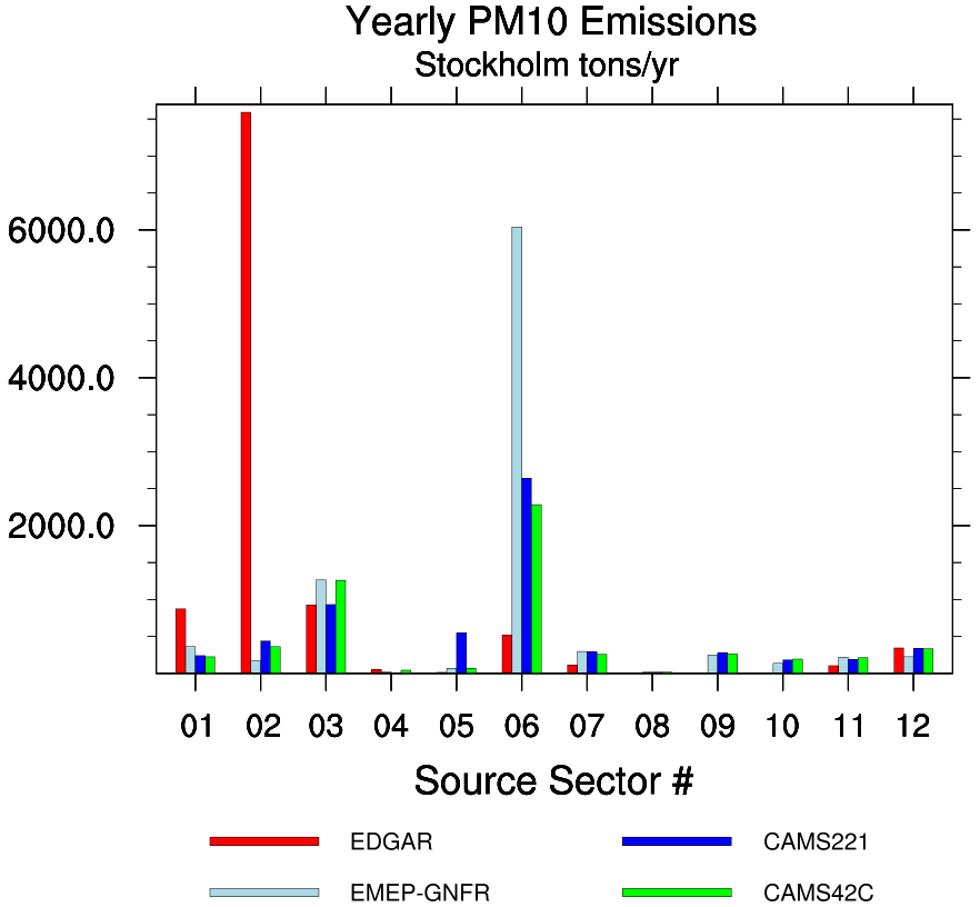
Figure 4Total PM10 emissions (in t yr−1) for Stockholm for EDGAR (red), EMEP-GNFR (light blue), CAMS221 (blue) and CAMS42C (green) for each GNFR sector.
Another reason for these differences is the spatial distribution of the emissions which differ from one inventory to the other (see Fig. S1 in the Supplement).
As mentioned before, CAMS42C includes condensables leading to larger PM10 potentials than CAMS221. Despite the overall increase in PPM emissions caused by the inclusion of condensables in CAMS42C, emissions remain lower than the median in cities like Stockholm (red circle in Fig. 3d). For Malopolska the potential is larger for EDGAR and CAMS42C (see also Fig. S2), partly caused by larger emissions.
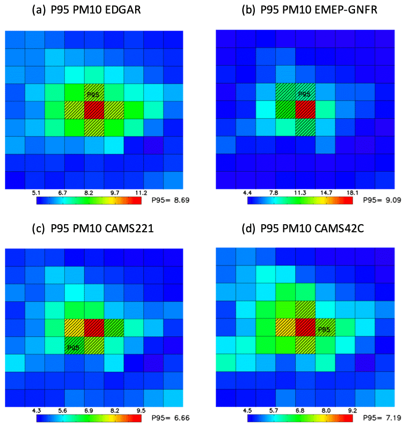
Figure 5Overview of the location of the P95 values for the calculated PM10 concentrations (in µg m−3) by the four base cases for the domain STO. Shaded grid cells indicate the location of the values above the P95 by (a) EDGAR, (b) EMEP-GNFR, (c) CAMS221 and (d) CAMS42C. The number next to P95 represents the average of the P95 values.
Apart from the vertical and spatial distribution of the emissions, another reason for differences in potentials might be related to the fact that the location of the P95 (95th percentile) value cells where the concentration changes are calculated differ for each model, as shown in Fig. 5. More specifically, the P95 values might be positioned at different locations in the four base cases (shaded grid cells in Fig. 5).
PM10 includes not only primary particles but also secondary particles. Secondary particles are formed by gases reacting (such as NOx, VOC and SOx) and condensing (gas to particle conversion) onto pre-existing particles or by nucleation.
In the next section we analyse the impact of aerosol secondary precursors reductions on calculated PM10 concentrations.
3.3.2 NOx
Compared with other precursors, NOx shows a good agreement among models with a couple of inconsistencies identified in Po Valley for EDGAR and CAMS42C, where the potencies are slightly larger than the 20 % threshold around the median. This good agreement can be explained by the fact that NOx emissions originate in great part from the transport sector, a sector for which the spatial proxies (for the spatial and sectorial disaggregation) are generally well described and harmonised among inventories (Trombetti et al., 2018). In addition, NOx sources are mostly diffuse (as opposed to point sources) and less subject to localised hot-spot differences.
3.3.3 SOx
For Stockholm large differences are found in EDGAR potentials when compared with the median (indicated by a red rectangle in Fig. 3a). The explanation for this is a strong overestimation of the SOx emissions (factor ∼10; Fig. 1c), which is partly compensated by an underestimation of the potency (factor ∼2). For MAD and BRU, we see that higher SOx emissions (factor ∼2) by EDGAR are compensated by lower potencies, which lead to overall similar potentials. Hence, reducing SOx emissions in EDGAR has a larger impact on PM10 concentrations when compared with the median, via the chemical reactions that lead to the formation of ammonium sulfate aerosol as described in De Meij et al. (2009b).
3.3.4 NH3
With the exception of EMEP-GNFR, all models show an inconsistency for NH3 in the Malopolska region. EDGAR shows higher emissions (factor ∼2) than the ensemble, but these higher emissions are compensated by lower potencies, which lead to overall similar potentials. CAMS221 and CAMS42C both show larger emissions too (although to a lesser extent than EDGAR) and lower potencies, leading to relatively similar potentials (green diamond symbols in Fig. 3). Note that given the reduced NH3 emissions in urban areas, these emissions do not lead to important potentials in many cities, and hence they do not appear in Fig. 3.
3.3.5 VOC
VOC potentials are generally too low (lower than the 20 % threshold detailed in Sect. 2.4) to appear in the figures, apart from Po Valley where CAMS221 shows a small inconsistency with respect to the median (orange squares in Fig. 3).
From the analysis of these different precursors, PPM appears to be the precursor leading to the major differences in terms of potentials, i.e. concentration change responses that are of direct relevance when designing air quality plans (Fig. S5). Although simpler to manage because of their linearity, they deserve more attention given their important variability (among models) and importance in terms of final concentrations.
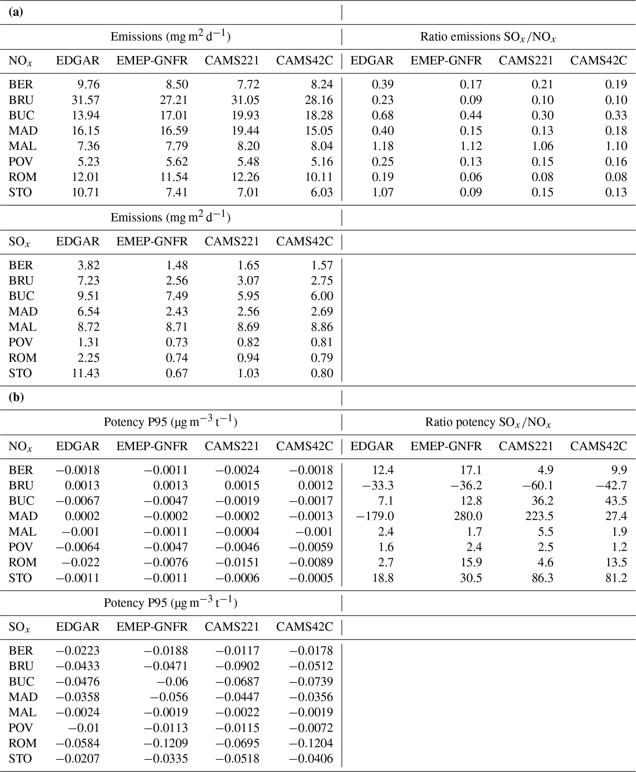
Table 2Part (a) is an overview of BaseCase emissions for NOx and SOx, together with the ratio in the emissions between these two pollutants. Part (b) is similar to (a) but for potency at P95.
3.3.6 ratios
To understand better the sensitivity of PM10 formation to NOx, SOx or NH3 reductions, we analyse the ratios between these precursors across inventories.
Table 2a shows the ratios between BaseCase domain averaged SOx and NOx emission densities. For example, the minimum ratio is around 0.06, indicating that there are around 16 times more NOx (11.5 mg m2 d−1) than SOx emissions (0.74 mg m2 d−1) in Rome for EMEP-GNFR. Table 2b shows, on the other hand, that the corresponding potency ratios are inverted, with much larger efficiencies when reducing SOx than NOx emissions. The same is true in most cities. This can be explained by the fact that NOx has to compete with NH3 to form PM, whereas SOx emission reductions directly lead to PM changes.
While this behaviour is quite general, there is a large variability in its magnitude. In some cities, such as Brussels, negative ratios appear to be caused by concentration increases when NOx emissions are reduced. This corroborates the findings by Clappier et al. (2021) who found that reducing SO2 emissions where abundant is always efficient and relatively linear, as shown also in the next section on non-linearities.
A similar analysis can be performed with NOx to NH3 ratios (see Table S4). NOx to NH3 contribute to the formation of ammonium nitrate aerosol – via the reactions NO2 + OH → HNO3 – which reacts (when there is sufficient ammonia available to neutralise all sulfate) with NH3 to form NH4NO3 aerosol, a fraction of PM10. Details on the chemical pathways can be found in Thunis et al. (2021a). As an example, the emission ratio for Rome by EDGAR is 3.3, while the corresponding numbers are 4.9, 5.4 and 4.8 for EMEPC, CAMS42C and EMEP-GNFR, respectively. While NOx emissions in the four inventories are similar, EDGAR contains almost a factor 2 more NH3 emissions. This means that NH3 is relatively more abundant in EDGAR and its reduction has therefore less impact on concentration. This results in the formation processes being more “NOx sensitive” in Rome. Thus, reducing NOx in EDGAR leads to a larger impact on PM10 concentrations.
Table 3Absolute potential (50 %) divided by the absolute potential (25 %) for PM10 when NOx emissions are reduced by 50 % and 25 % for 95th percentile (P95) values. Numbers with a ratio higher than 3 % compared with the PPM 50 % potential P95 values are shown.
3.3.7 Non-linearities
Non-linearity in PM responses to emission changes often results from changes in chemical regimes where the formation process is limited by a different species.
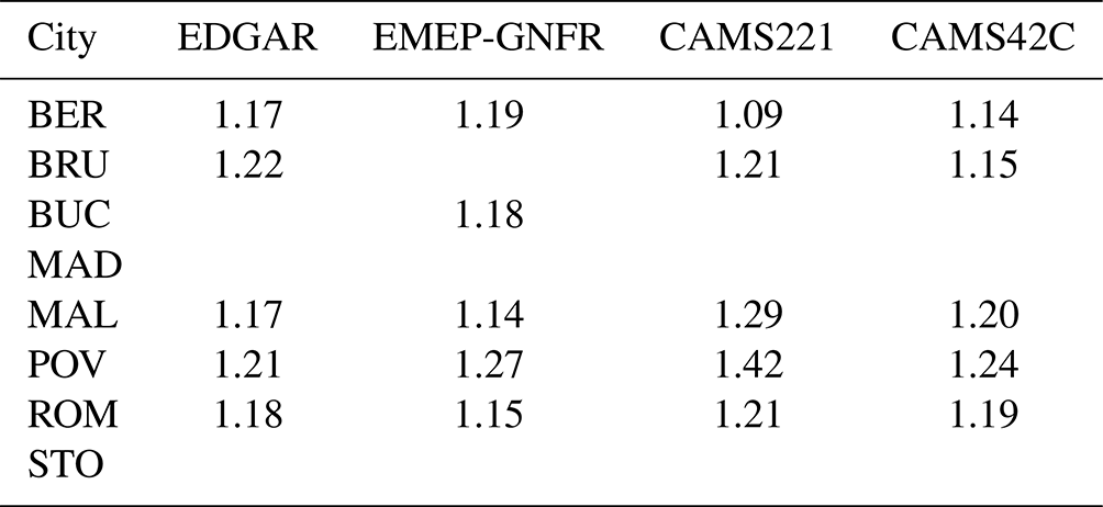
Analysing the absolute potentials ratio (50 % vs. 25 %) in Tables 3–7 provides information on the (non-)linearity of the relationship between emission and concentration changes. If the ratio is close to 1.00, then there is linear correlation between the two. Departure from 1 indicates non-linearity. We only show the ratios which are 3 % or higher when compared with the 50 % potential for PPM in order to highlight the most relevant ratios.
For primary PM (PM2.5 and PMcoarse) we get a linear relationship as expected (see Table 6). The reason for this is that primary emissions only affect the primary part of the aerosol formation and do not undergo chemical reactions.
For NOx (Table 3) the behaviour is generally non-linear with ratios larger than 1.00. This indicates that calculated PM10 concentrations would be reduced more between 25 % and 50 % than between 0 % and 25 %. For example, EDGAR indicates 1.18 in Rome, indicating that PM10 concentrations would be reduced by 18 % more between 25 % and 50 % than between 0 % and 25 %. This might be explained by a change in chemical regime from an NH3-limited regime (when NOx is more abundant and less efficient) to a NOx-limited regime (NOx is less abundant and more efficient) as emissions are reduced further.
Note the importance of averaging processes on the indicator value. Based on the 95th percentile locations, the ratio for Bucharest with EMEP-GNFR is 1.18, whereas for domain-averaged values the ratio becomes 1.08 indicating closer to linear relationships. This corroborates the results by Thunis et al. (2021c), who assessed the contribution of cities to their own air pollution. They showed that the type of indicator impacts the final outcome, i.e. the share of the city pollution caused by a city's own emissions. It also confirms that indicators based on averaged values tend to report more linear relationships.
Table 4Absolute potential (50 %) divided by the absolute potential (25 %) for PM10 when VOC emissions are reduced by 50 % and 25 % for 95th percentile (P95) values. Numbers with a ratio higher than 3 % compared with the PPM 50 % potential P95 values are shown.
For VOC (Table 4) and SOx (not shown, as the ratios compared with the PPM are less than 3 %) we find that ratios remain very close to 1.00.
NH3 shows significant non-linearity with ratios larger than 1 (Table 5). The same explanations as for NOx can be used to explain the larger efficiency of emission reductions when these emissions are reduced further in an NH3-limited regime.
Finally, a similar ratio can be constructed for emission reductions that include all species together (SOx, NOx, VOC, NH3, PM2.5 and PMcoarse). The results generally indicate a linear behaviour mainly because of compensating effects (NOx non-linearities are weakened by other emitted species), with the exception of EMEP-GNFR in Berlin and BUC. For these two locations, the explanation lies in the much lower PPM emissions (linear) and larger NOx emissions (non-linear). Clappier et al. (2021) showed which chemical regimes are responsible to the secondary inorganic PM formation over Europe and how these chemical regimes can help in designing efficient PM abatement strategies. They showed that during winter, PM2.5 concentrations are predominantly NH3 sensitive in most of Europe. During summer, PM2.5 are predominantly SO2 sensitive in most of Europe.
Table 5Absolute potential (50 %) divided by the absolute potential (25 %) for PM10 when NH3 emissions are reduced by 50 % and 25 % for 95th percentile (P95) values. Numbers with a ratio higher than 3 % compared with the PPM 50 % potential P95 values are shown.
3.4 Variability in ozone BaseCase concentrations
Ozone is chemically formed by the oxidation process of volatile organic compounds in the presence of NOx (NO + NO2), and its formation is driven by sunlight intensity. At the same time, NOx also works as an ozone sink through NOx titration (NO+O3 → NO2+ O2) that occurs during the night and during winter, i.e. fewer photolysis reactions of NO2 (Jhun et al., 2015) and O3 are removed by NO emissions from road traffic in city centres (Sharma et al., 2016).
Figure 6 shows that yearly averaged O3 concentrations are very similar.
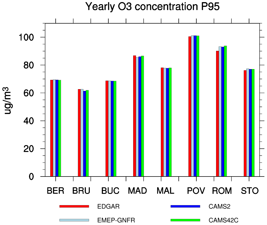
Figure 6Yearly average O3 concentrations by EDGAR (red), EMEP-GNFR (light blue), CAMS221 (blue) and CAMS42C (green) for the eight locations (Berlin, Brussels, Bucharest, Madrid, Malopolska region, Po Valley region, Rome and Stockholm). The concentrations represent values above the 95th percentile values, showing the highest 5 % values in the domain from the BaseCase.
Table 6Absolute potential (50 %) divided by the absolute potential (25 %) for PM10 when PM2.5 and PMcoarse emissions are reduced by 50 % and 25 % for 95th percentile (P95) values.
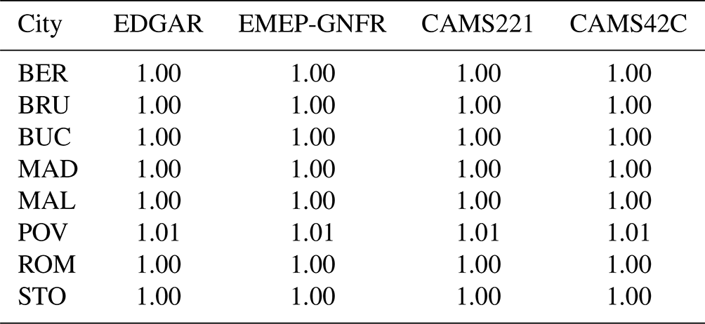
Table 7Absolute potential (50 %) divided by the absolute potential (25 %) for PM10 when the emissions of all pollutants (SOx, NOx, VOC, NH3, PM2.5 and PMcoarse) are reduced together by 50 % and 25 % for 95th percentile (P95) values.
3.5 Analysis of potentials and potencies for O3
In Fig. 7 we analyse the impact of the reduction in NOx and VOC on calculated O3 concentrations for the different locations.
The production of O3 depends on the availability of NOx and VOCs, which are emitted mostly from sectors such as industry and road transport. For that reason, only NOx and VOC appear in Fig. 7, except for NH3 for EDGAR. The latter can be explained by the fact that NH3 contributes to the formation of secondary aerosol and decreases the acidity of the aerosols. The aerosol pH plays an important role in the reactive uptake and release of gases, which can affect ozone chemistry (Pozzer et al., 2017). This NH3 impact also exists for the other inventories but is lower than the 20 % threshold and therefore does not appear in the diamond plots.
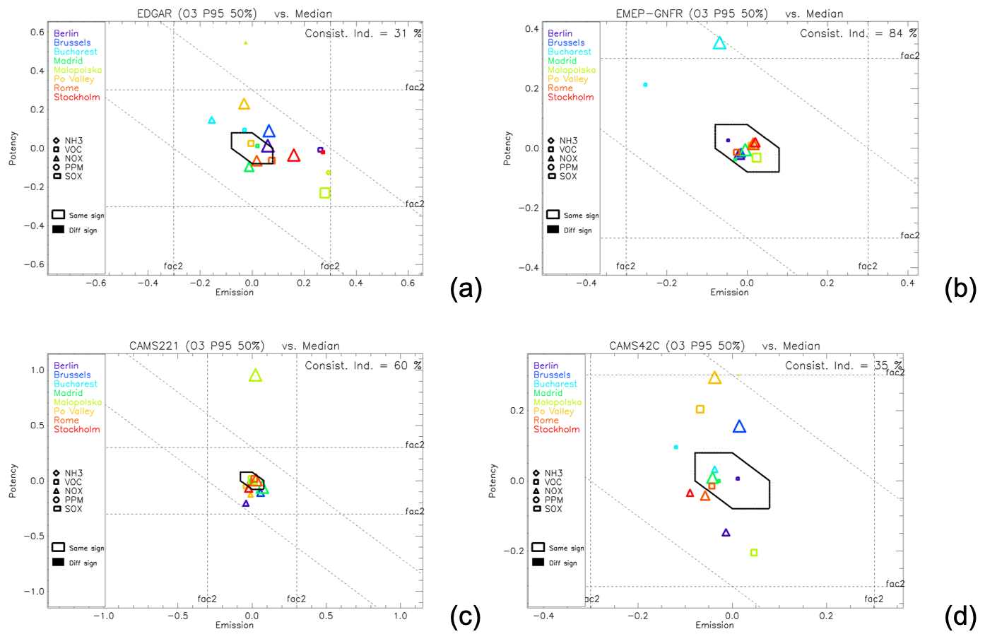
Figure 7Diamond plot for O3 concentrations for (a) EDGAR, (b) EMEP-GNFR, (c) CAMS221 and (d) CAMS42C. The values represent values above the 95th percentile, showing the highest 5 % values in the domain from the BaseCase. The x and y axes are expressed as logarithms. For each city, the size of a symbol is proportional to the maximum absolute potential of the considered precursor, across models. Note that symbols for which emissions are relevant and that characterise the median all fall at the (0, 0) position. For visualisation purposes, these symbols have been slightly shifted within the diamond shape.
3.5.1 VOC
With the exception of CAMS221, all models show some differences with the median for VOC (Fig. 7). In Maloposka, Stockholm and Berlin, EDGAR emissions are a factor ∼2 higher than the median value, whereas in the first location, the lower potencies compensate for these emission differences, leading to similar potentials. This is not the case for the two latter cities, where similar potencies lead to larger potentials. For EMEP-GNFR, only Bucharest shows differences with lower emissions and higher potencies, leading to similar potentials. It is interesting to note the large differences between CAMS221 and CAMS42C. While the addition of condensables in CAMS42C does not impact O3 formation, other changes included in version CAMS42C have significant impacts. While NOx responses dominate in most cases in CAMS221, this is not the case in CAMS42C where VOC responses become important for three cities. Differences with the median are mostly caused by potency rather than by emission differences. Thus, it is interesting that a change in version can lead to very important changes in model responses despite similar absolute O3 levels.
Note that VOC appears systematically as an important impact (visible in Fig. 7) for Malopolska and Po Valley, whereas this is not the case systematically for the other locations. The reason is that for these two regions, emissions are reduced over larger areas, leading to larger impacts. (More details on the potentials and potencies for the different locations can be found in Figs. S6–S8.)
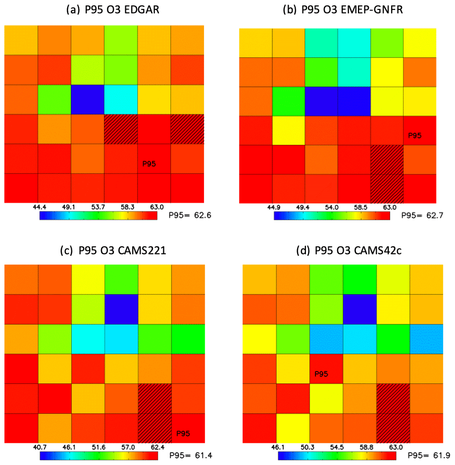
Figure 8Overview of the location of the P95 values for the calculated O3 concentrations (in µg m−3) by the four base cases for the domain BRU. Shaded grid cells indicate the location of values above the P95 values by (a) EDGAR, (b) EMEP-GNFR, (c) CAMS221 and (d) CAMS42C. The number next to P95 represents the average of the P95 values.
3.5.2 NOx
NOx shows generally larger impacts than VOC (see Fig. S9). While for PM10, NOx responses were shown in the previous section to be consistent among models, this is not the case for O3. Potential differences originate mostly from differences in potencies, while emissions remain relatively similar among inventories. The largest differences occur for Bucharest (EMEP-GNFR), Malopolska and Po Valley (CAMS42C) with much larger potency estimates than the median, indicating that these regions are more sensitive to NOx reduction than for other inventories. However, opposite trends also occur as in Berlin for CAMS221 and CAMS42C. It is also interesting to note that in some cities, such as Brussels, differences in model versions (CAMS42C vs. CAMS221) significantly affect the NOx responses (as already noted for VOC).
In Malopolska, EDGAR and CAMS42C show a change in sign in terms of responses. In such cases, NOx reductions lead to an O3 increase, whereas the median shows an opposite behaviour.
The highest consistency (84 %) with the ensemble is found for EMEP-GNFR, meaning that 84 % of the relevant impacts (delta concentrations) are within the 20 % limit, indicating that EMEP-GNFR is often picked as the median. On the other hand, CAMS42C and EDGAR show the lowest consistency value. It is interesting to note the large difference between the two versions of the same inventory (60 % vs. 35 % for CAMS221 and CAMS42C, respectively).
Similarly to PM10, some of the differences are partly explained by the location of the P95 values that are not similar for the four inventories, as shown in Fig. 8, where EDGAR locations differ from all others (shaded grid cells).
Table 8Part (a) is an overview of BaseCase emissions (in mg m2 d−1) for NOx and VOC, together with the ratio in the emissions between these two pollutants. Part (b) is similar to (a) but for potency at P95 (in mg m−3).
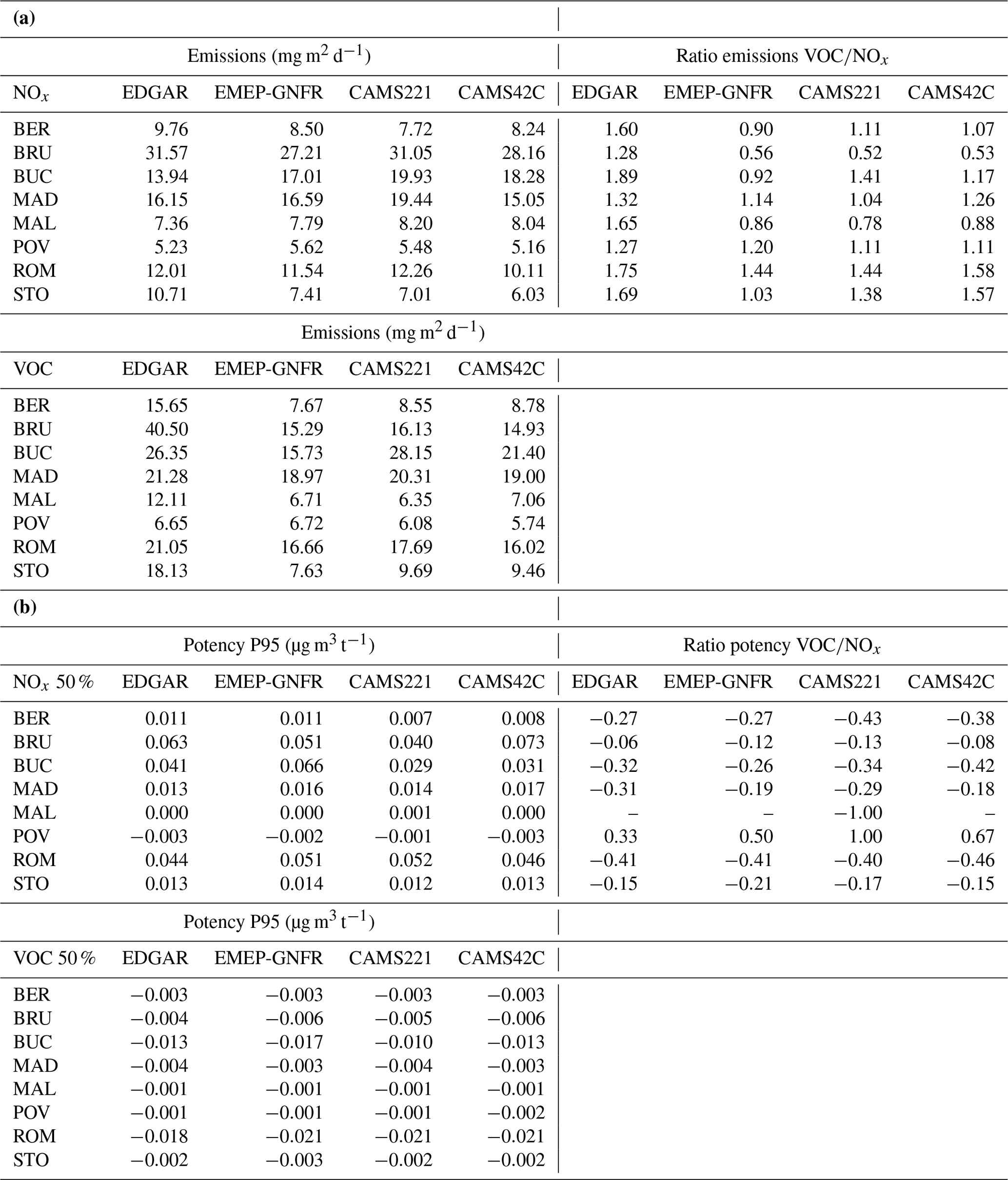
3.5.3 VOC/NOx ratios
To understand better the impact of NOx and VOC reductions on the production or loss of O3, and the interconnections between the two, we analyse the ratio for the different inventories in Table 8a. For Malopolska, Bucharest or Brussels, the emission ratio for EDGAR is twice as large than the others. This reflects in the EMEP-GNFR diagram (Fig. 7b) where these cities show clear inconsistencies. The larger amount of VOC in these cities does not impact significantly the potencies (Table 8b). While NOx potencies are mostly positive, indicating an increase in the O3 concentrations over the urban areas, VOC potencies are always negative, indicating lower O3 concentrations when reducing VOC emissions. Differences in ratios might lead to changes in the chemical regime, which would explain some of the differences in the potentials.
The differences in ratios between the four emission inventories highlight the importance of the accuracy of emission inventories, which could strongly impact the chemical regime (i.e. NOx limited or VOC limited). Even moderate perturbations in NOx or VOC emissions could change the chemical regime of O3 formation (Xiao et al., 2010).
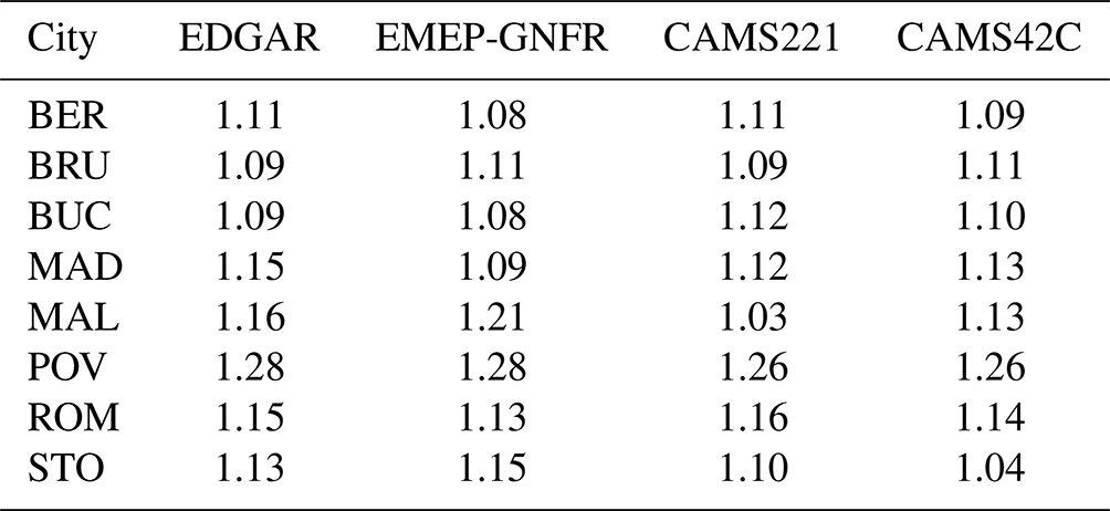
Table 9Absolute potential (50 %) divided by the absolute potential (25 %) for O3 when NOx emissions are reduced by 50 % and 25 % for 95th percentile (P95) values.
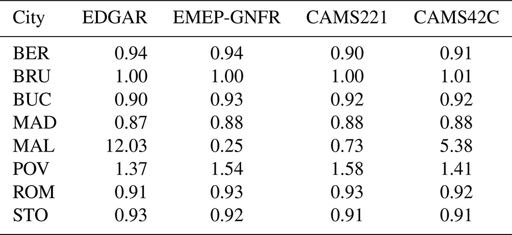
3.5.4 Non-linearities
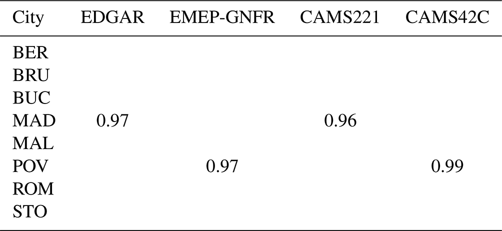
Previous studies (Cohan et al., 2005; Xiao et al., 2010) have shown that the formation of ozone is more sensitive to large reductions in NOx that depart from a linear emission scaling. To this end, we show in Tables 9 and 10 the ratio between absolute potentials (at 50 % and 25 %) for P95, which help to assess the level of non-linearity of the atmospheric reactions that involve gaseous precursors NOx and VOCs in the formation of ozone. Table 9 shows large non-linearities when NOx emissions are reduced. A number larger than 1 indicates superlinearity, which means that O3 concentrations are more reduced between 25 % and 50 % than between 0 % and 25 %. For Malopolska, we find a large ratio for EDGAR (12.03) because it is based on small values (−0.325 vs. −0.027).
Table 10Absolute potential (50 %) divided by the absolute potential (25 %) for O3 when VOC emissions are reduced by 50 % and 25 % for 95th percentile (P95) values.
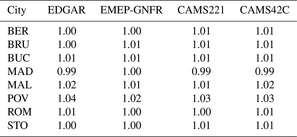
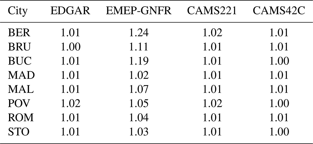
Table 11Absolute potential (50 %) divided by the absolute potential (25 %) for O3 when NOx and VOC emissions are reduced together by 50 % and 25 % for 95th percentile (P95) values.
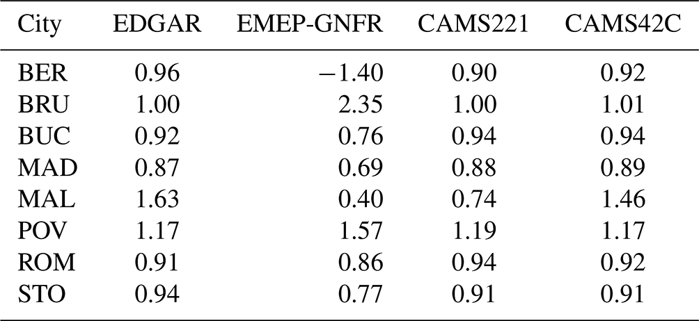
Ratios are generally lower than one, with the clear exception in Po Valley. This must be put in relation with the fact that Po Valley is the only place where potencies are negative (see Table 8b), indicating a different chemical regime (O3 formation) than in other locations (O3 titration). This is explained by the fact that the Po Valley domain includes suburban and background areas where O3 formation takes place.
For VOC the ratios are close to 1.00 indicating a linear behaviour (Table 10). This corroborates previous studies (Xiao et al., 2010).
Reducing NOx and VOC emissions together (Table 11) also shows some non-linear behaviour that originates from the NOx side. The formation of O3 is less sensitive to the reduction in NOx emissions when VOC emissions are simultaneously reduced. This corroborates the findings of Xiao et al. (2010) and Xing et al. (2017).
In this work, we assessed how emissions impact the model BaseCase concentrations but also concentration changes when emission reductions are applied. The impact of emission reductions based on four emission inventories (EDGAR 5.0, EMEP-GNFR, CAMS version 2.2.1 and CAMS version 4.2 + condensables) has been investigated for PM10 and O3 in eight cities and regions in Europe. We assessed the model's variability in terms of model responses to emission changes with the support of specific indicators (potentials and potencies) and used a screening method adapted from Thunis et al. (2022) to identify the main inconsistencies among model responses. A median value has been constructed to serve as reference for the comparisons.
Our study reveals that the impact of reducing aerosols (precursors), such as PPM, NOx, SO2, NH3 and VOCs, result in different potentials and potencies, differences that are mainly explained by differences in emission quantities, differences in their spatial distributions as well as differences in their sector allocation. The main findings are the following:
-
In general, the variability among models is larger for concentration changes (potentials) than for absolute concentrations. This is true for both PM10 and O3.
-
Emission densities at each location for all precursors are quite consistent, apart from EDGAR which generally shows larger urban scale emissions.
-
Similar emissions can, however, hide large variations in sectorial allocation. Our results stress the importance of the sectorial repartition of the emissions, given their different vertical distribution (emissions in the industrial sector are emitted at higher levels and have less impact on surface concentration) especially for PPM. This sectorial allocation can lead to large impacts on potency. For similar reasons, larger emissions do not necessarily lead to larger potencies. At the local scale, it is therefore important to further work on the modelling of PPM and on the estimate of its underlying emissions.
-
PPM appears to be the precursor leading to the major differences in terms of potentials, i.e. in terms of PM10 concentration changes. This is of direct relevance when designing air quality plans. Although simpler to manage because of their linearity, they would deserve more attention at the local scale given their importance in terms of final concentrations and their large variability (among models). Additional efforts to check the consistency and accuracy of the PPM emissions and their sectorial share is therefore important to ensure robust model responses.
-
For O3, NOx emission reductions are the most efficient, likely because of the urban focus of this work and the abundance of NOx emissions in this type of area.
-
In terms of non-linear behaviour, the relationship between emission reduction and PM10 concentration change shows the largest non-linearity for NOx and, to a lesser extent, for NH3, whereas it remains mostly linear for the other precursors (VOC, SOx and PPM). Potentials based on a single emission reduction value are therefore, most of the time, not sufficient and do not provide a complete view of the non-linear behaviour of the emission reductions. Additional NOx emission reductions are necessary to better understand the non-linearity of reducing VOC and NOx reductions together.
-
In terms of non-linear behaviour, the relationship between emission reduction and O3 concentration change shows the largest non-linearity for NOx (concentration increase) and a quasi-linear behaviour for VOC (concentration decrease). Similar to above, potentials based on a single emission reduction value for NOx are not always sufficient to understand the non-linear behaviour of emission reductions.
-
Potencies and potentials can show differences that are as large between inventories (CAMS221 vs. EMEP-GNFR) as between inventory versions (CAMS221 vs. CAMS42C). This is the case, for example, in Brussels for the NOx responses to PM10 concentrations.
-
Precursor emission ratios (e.g. for ozone or for PM10) show important differences among emission inventories. This emphasises the importance of the accuracy of emission estimates since these differences can lead to changes in chemical regimes, directly affecting the responses of O3 or PM10 concentrations to emission reductions.
-
It is also important to understand that the choice of the indicator used in a given analysis (for example, mean or percentile values) can lead to different outcomes. It is therefore important to assess the variability in the results around the choice of the indicator to avoid misleading interpretations of the results.
From an emission inventory viewpoint, this work indicates that the most efficient actions to improve the robustness of the modelling responses to emission changes would be to better assess the sectorial share and total quantities of PPM emissions. Another important aspect is to better assess emitted precursor ratios as these lead to important differences in terms of model responses, both in the case of O3 ( ratio) and PM ( ratios). From a modelling point of view, NOx responses are the more challenging and require caution because of their non-linearity.
The source code of the screening method of the statistical analysis can be found here: https://doi.org/10.5281/zenodo.8082531 (De Meij et al., 2023). The emission data can be downloaded here: https://eccad.sedoo.fr/ (last access: 23 January 2024).
The supplement related to this article is available online at: https://doi.org/10.5194/gmd-17-587-2024-supplement.
AdM and PT wrote the manuscript draft. PT developed the code. AdM, PT and CC produced the data. AdM, PT and CC analysed the data. EP and BB reviewed and edited the manuscript.
The contact author has declared that none of the authors has any competing interests
Publisher’s note: Copernicus Publications remains neutral with regard to jurisdictional claims made in the text, published maps, institutional affiliations, or any other geographical representation in this paper. While Copernicus Publications makes every effort to include appropriate place names, the final responsibility lies with the authors.
The emission inventories have been provided by the Emissions of atmospheric Compounds and Compilation of Ancillary Data (ECCAD) system (https://eccad.aeris-data.fr; last access: 19 January 2024).
This paper was edited by Jason Williams and reviewed by two anonymous referees.
Amann, M., Bertok, I., Borken-Kleefeld, J., Cofala, J., Heyes, C., Höglund-Isaksson, L., Klimont, Z., Nguyen, B., Posch, M., Rafaj, P., Sandler, R., Schöpp, W., Wagner, F., and Winiwarter, W.: Cost-effective control of air quality and greenhouse gases in Europe: Modeling and policy applications, Environ. Modell. Softw., 26, 1489–1501, https://doi.org/10.1016/j.envsoft.2011.07.012, 2011.
Cheewaphongphan, P., Chatani, S., and Saigusa, N.: Exploring Gaps between Bottom-Up and Top-Down Emission Estimates Based on Uncertainties in Multiple Emission Inventories: A Case Study on CH4 Emissions in China, Sustainability, 11, 2054, https://doi.org/10.3390/su11072054, 2019.
Clappier, A., Thunis, P., Beekmann, M., Putaud, J. P., and De Meij, A.: Impact of SOx, NOx and NH3 emission reductions on PM2.5 concentrations across Europe: Hints for future measure development, Environ. Int., 156, 0160-4120, https://doi.org/10.1016/j.envint.2021.106699, 2021.
Cohan, D. S., Hakami, A., Hu, Y. T., and Russell, A. G.: Nonlinear response of ozone to emissions: Source apportionment and sensitivity analysis, Environ. Sci. Technol., 39, 6739–6748, https://doi.org/10.1021/es048664m, 2005.
Crippa, M., Guizzardi, D., Muntean, M., Schaaf, E., Dentener, F., van Aardenne, J. A., Monni, S., Doering, U., Olivier, J. G. J., Pagliari, V., and Janssens-Maenhout, G.: Gridded emissions of air pollutants for the period 1970–2012 within EDGAR v4.3.2, Earth Syst. Sci. Data, 10, 1987–2013, https://doi.org/10.5194/essd-10-1987-2018, 2018.
Crippa, M., Solazzo, E., Huang, G., Guizzardi, D., Koffi, E., Muntean, M., Schieberle, C., Friedrich, R., and Janssens-Maenhout, G.: High resolution temporal profiles in the Emissions Database for Global Atmospheric Research, Sci. Data, 7, 121, https://doi.org/10.1038/s41597-020-0462-2, 2020.
De Meij, A., Wagner, S., Gobron, N., Thunis, P., Cuvelier, C., Dentener, F., and Schaap, M.: Model evaluation and scale issues in chemical and optical aerosol properties over the greater Milan area (Italy), for June 2001, Atmos. Res., 85, 243–267, 2007.
de Meij, A., Gzella, A., Cuvelier, C., Thunis, P., Bessagnet, B., Vinuesa, J. F., Menut, L., and Kelder, H. M.: The impact of MM5 and WRF meteorology over complex terrain on CHIMERE model calculations, Atmos. Chem. Phys., 9, 6611–6632, https://doi.org/10.5194/acp-9-6611-2009, 2009a.
De Meij, A., Thunis, P., Bessagnet, B., and Cuvelier, C.: The sensitivity of the CHIMERE model to emissions reduction scenarios on air quality in Northern Italy, Atmos. Environ., 43, 1897–1907, 2009b.
De Meij, A., Bossioli, E., Vinuesa, J. F., Penard, C., and Price, I.: The effect of SRTM and Corine Land Cover on calculated gas and PM10 concentrations in WRF-Chem, Atmos. Environ., 101, 177–193, 2015.
De Meij, A., Zittis, G., and Christoudias, T.: On the uncertainties introduced by land cover data in high-resolution regional simulations, Meteorol. Atmos. Phys., 1213–1223, https://doi.org/10.1007/s00703-018-0632-3, 2018.
De Meij, A., Astorga, C., Thunis, P., Crippa, M., Guizzardi, D., Pisoni, E., Valverde, V., Suarez-Bertoa, R., Oreggioni, G. D., Mahiques, O., and Franco, V.: Modelling the Impact of the Introduction of the EURO 6d-TEMP/6d Regulation for Light-Duty Vehicles on EU Air Quality, Appl. Sci.-Basel, 12, 4257, https://doi.org/10.3390/app12094257, 2022.
De Meij, A., Cuvelier, C., Thunis, P., Pisoni, E., and Bessagnet, B.: Sensitivity of air quality model responses to emission changes: comparison of results based on four EU inventories through FAIRMODE benchmarking methodology, Zenodo [code], https://doi.org/10.5281/zenodo.8082531, 2023.
European Commission: Proposal for a DIRECTIVE OF THE EUROPEAN PARLIAMENT AND OF THE COUNCIL on ambient air quality and cleaner air for Europe, COM (2022) 542 final, 2022/0347 (COD), October 2022.
European Environment Agency: Air quality in Europe – 2020 report, EEA report No. 09/2020, https://www.eea.europa.eu/publications/air-quality-in-europe-2020-report (last access: 19 January 2024), 2020.
Fagerli, H., Simpson, D., and Tsyro, S.: Unified EMEP model: Updates, in: EMEP Status Report 1/2004, Transboundary acidification, eutrophication and ground level ozone in Europe, Status Report 1/2004, The Norwegian Meteorological Institute, Oslo, Norway, 11–18, 2004.
Georgiou, G. K., Kushta, J., Christoudias, T., Proestos, Y., and Lelieveld, J.: Air quality modelling over the eastern Mediterranean: seasonal sensitivity to anthropogenic emissions, Atmos. Environ., 222, https://doi.org/10.1016/j.atmosenv.2019.117119, 2020.
Granier, C., Darras, S., Denier van der Gon, H., Doubalova, J., Elguindi, N., Galle, B., Gauss, M., Guevara, M., Jalkanen, J.-P., Kuenen, J., Liousse, C., Quack, B., Simpson, D., and Sindelarova, K.: The Copernicus Atmosphere Monitoring Service Global and Regional Emissions (April 2019 Version), Copernicus Atmosphere Monitoring Service, (CAMS) report, https://doi.org/10.24380/d0bn-kx16, 2019.
Janssens-Maenhout, G., Crippa, M., Guizzardi, D., Muntean, M., Schaaf, E., Dentener, F., Bergamaschi, P., Pagliari, V., Olivier, J. G. J., Peters, J. A. H. W., van Aardenne, J. A., Monni, S., Doering, U., Petrescu, A. M. R., Solazzo, E., and Oreggioni, G. D.: EDGAR v4.3.2 Global Atlas of the three major greenhouse gas emissions for the period 1970–2012, Earth Syst. Sci. Data, 11, 959–1002, https://doi.org/10.5194/essd-11-959-2019, 2019.
Jhun, I., Coull, B. A., Zanobetti, A., and Koutrakis, P: The impact of nitrogen oxides concentration decreases on ozone trends in the USA, Air Qual. Atmos. Hlth., 283–292, https://doi.org/10.1007/s11869-014-0279-2, 2015.
Kuenen, J., Dellaert, S., Visschedijk, A., Jalkanen, J.-P., Super, I., and Denier van der Gon, H.: Copernicus Atmosphere Monitoring Service regional emissions version 4.2 (CAMS-REG-v4.2) Copernicus Atmosphere Monitoring Service, ECCAD, https://doi.org/10.24380/0vzb-a387, 2021.
Kuenen, J., Dellaert, S., Visschedijk, A., Jalkanen, J.-P., Super, I., and Denier van der Gon, H.: CAMS-REG-v4: a state-of-the-art high-resolution European emission inventory for air quality modelling, Earth Syst. Sci. Data, 14, 491–515, https://doi.org/10.5194/essd-14-491-2022, 2022.
Kuenen, J. J. P., Visschedijk, A. J. H., Jozwicka, M., and Denier van der Gon, H. A. C.: TNO-MACC_II emission inventory; a multi-year (2003–2009) consistent high-resolution European emission inventory for air quality modelling, Atmos. Chem. Phys., 14, 10963–10976, https://doi.org/10.5194/acp-14-10963-2014, 2014.
Logan, J. A.: An analysis of ozonesonde data for the troposphere: Recommendations for testing 3-D models and development of a gridded climatology for tropospheric ozone, J. Geophys. Res., 10, 16115–16149, 1998.
Mareckova, K., Pinterits, M., Ullrich, B., Wankmueller, R., and Mandl, N.: Review of emission data reported under the LRTAP Convention and NEC Directive Centre Emission Inventories Project, Technical Report 4/2018, CEIP, https://www.ceip.at/fileadmin/inhalte/ceip/00_pdf_other/2018/inventoryreport_2018.pdf, (last access: 19 Jauary 2024), 2018.
Miranda, A., Silveira, C., Ferreira, J., Monteiro, A., Lopes, D., Relvas, H., Borrego, C., and Roebeling, P.: Current air quality plans in Europe designed to support air quality management policies, Atmos. Pollut. Res., 6, 434–443, https://doi.org/10.5094/APR.2015.048, 2015.
Mircea, M., Bessagnet, B., D'Isidoro, M., Pirovano, G., Aksoyoglu, S., Ciarelli, G., Tsyro, S., Manders, A., Bieser, J., Stern, R., García Vivanco, M., Cuvelier, C., Aas, W., Prévôt, A. S. H., Aulinger, A., Briganti, G., Calori, G., Cappelletti, A., Colette, A., Couvidat, F., Fagerli, H., Finardi, S., Kranenburg, R., Rouïl, L., Silibello, C., Spindler, G., Poulain, L., Herrmann, H., Jimenez, J. L., Day, D. A., Tiitta, P., and Carbone, S.: EURODELTA III exercise: An evaluation of air quality models' capacity to reproduce the carbonaceous aerosol, Atmos. Environ. X, 2, https://doi.org/10.1016/j.aeaoa.2019.100018, 2019.
Pozzer, A., Tsimpidi, A. P., Karydis, V. A., de Meij, A., and Lelieveld, J.: Impact of agricultural emission reductions on fine-particulate matter and public health, Atmos. Chem. Phys., 17, 12813–12826, https://doi.org/10.5194/acp-17-12813-2017, 2017.
Sharma, S., Sharma, S., Khare, M., and Kwatra, S.: Statistical behavior of ozone in urban environment, Sustain. Env. Res., 26, 142–148, https://doi.org/10.1016/j.serj.2016.04.006, 2016.
Simpson, D., Fagerli, H., Jonson, J., Tsyro, S., Wind, P., and Tuovinen, J.-P.: The EMEP Unified Eulerian Model. Model Description, EMEP MSC-W Report 1/2003, The Norwegian Meteorological Institute, Oslo, Norway, ISSN 0806-4520, 2003.
Simpson, D., Benedictow, A., Berge, H., Bergström, R., Emberson, L. D., Fagerli, H., Flechard, C. R., Hayman, G. D., Gauss, M., Jonson, J. E., Jenkin, M. E., Nyíri, A., Richter, C., Semeena, V. S., Tsyro, S., Tuovinen, J.-P., Valdebenito, Á., and Wind, P.: The EMEP MSC-W chemical transport model – technical description, Atmos. Chem. Phys., 12, 7825–7865, https://doi.org/10.5194/acp-12-7825-2012, 2012.
Vautard, R., Builtjes, P. H. J., Thunis, P., Cuvelier, C., Bedogni, M., Bessagnet, B., Honoré, C., Moussiopoulos, N., Pirovano, G., Schaap, M., Stern, R., Tarrason, L., and Wind, P.: Evaluation and intercomparison of Ozone and PM10 simulations by several chemistry transport models over four European cities within the CityDelta project, Atmos. Environ., 41, 173–188, https://doi.org/10.1016/j.atmosenv.2006.07.039, 2007.
Thunis, P., Rouil, L., Cuvelier, C., Stern, R., Kerschbaumer, A., Bessagnet, B., Schaap, M., Builtjes, P., Tarrason, L., Douros, J., Moussiopoulos, N., Pirovano, G., and Bedogni, M.: Analysis of Model Responses to Emission-reduction Scenarios within the CityDelta Project, Atmos. Environ., 41, 208–220, https://doi.org/10.1016/j.atmosenv.2006.09.001, 2007.
Thunis, P., Cuvelier, C., Roberts, P., White, L., Nyrni, A., Stern, R., Kerschbaumer, A., Bessagnet, B., Bergstrom, R., and Schaap, M.: EURODELTA – Evaluation of a Sectoral Approach to Integrated Assessment Modeling – Second Report, EUR 24474 EN, Luxembourg (Luxembourg), Publications Office of the European Union, https://doi.org/10.2788/40803, 2010.
Pernigotti, D., Thunis, P., Cuvelier, C., Georgieva, E., Gsella, A., De Meij, A., Pirovano, G., Balzarini, A., Riva, G. M., Carnevale, C., Pisoni, E., Volta, M., Bessagnet, B., Kerschbaumer, A., Viaene, P., De Ridder, K., Nyiri, A., and Wind, P.: POMI: a model inter-comparison exercise over the Po Valley, Air Qual. Atmos. Health, 6, 701–715, https://doi.org/10.1007/s11869-013-0211-1, 2013.
Thunis, P., Clappier, A., Pisoni, E., and Degraeuwe, B.: Quantification of non-linearities as a function of time averaging in regional air quality modeling applications, Atmos. Environ., 103, 1352–2310, https://doi.org/10.1016/j.atmosenv.2014.12.057, 2015a.
Thunis, P., Pisoni, E., Degraeuwe, B., Kranenburg, R., Schaap, M., and Clappier, A.: Dynamic evaluation of air quality models over European regions, Atmos. Environ., 111, 1352–2310, https://doi.org/10.1016/j.atmosenv.2015.04.016, 2015b.
Thunis, P., Clappier, A., Beekmann, M., Putaud, J. P., Cuvelier, C., Madrazo, J., and de Meij, A.: Non-linear response of PM2.5 to changes in NOx and NH3 emissions in the Po basin (Italy): consequences for air quality plans, Atmos. Chem. Phys., 21, 9309–9327, https://doi.org/10.5194/acp-21-9309-2021, 2021a.
Thunis, P., Crippa, M., Cuvelier, C., Guizzardi, D., De Meij, A., Oreggioni, G., and Pisoni, E.: Sensitivity of air quality modelling to different emission inventories: A case study over Europe, Atmos. Environ., 10, 100111, https://doi.org/10.1016/j.aeaoa.2021.100111, 2021b.
Thunis, P., Clappier, A., de Meij, A., Pisoni, E., Bessagnet, B., and Tarrason, L.: Why is the city's responsibility for its air pollution often underestimated? A focus on PM2.5, Atmos. Chem. Phys., 21, 18195–18212, https://doi.org/10.5194/acp-21-18195-2021, 2021c.
Thunis, P., Clappier, A., Pisoni, E., Bessagnet, B., Kuenen, J., Guevara, M., and Lopez-Aparicio, S.: A multi-pollutant and multi-sectorial approach to screening the consistency of emission inventories, Geosci. Model Dev., 15, 5271–5286, https://doi.org/10.5194/gmd-15-5271-2022, 2022.
Thunis, P., Kuenen, J., Pisoni, E., Bessagnet, B., Banja, M., Gawuc, L., Szymankiewicz, K., Guizardi, D., Crippa, M., Lopez-Aparicio, S., Guevara, M., De Meij, A., Schindlbacher, S., and Clappier, A.: Emission ensemble approach to improve the development of multi-scale emission inventories, EGUsphere [preprint], https://doi.org/10.5194/egusphere-2023-1257, 2023.
Trombetti, M., Thunis., P., Bessagnet, B., Clappier, A., Couvidat, F., Guevara, M., Kuenen J., and López-Aparicio, S.: Spatial inter-comparison of Top-down emission inventories in European urban areas, Atmos. Environ., 173, 1352–2310, https://doi.org/10.1016/j.atmosenv.2017.10.032, 2018.
World Health Organization: WHO global air quality guidelines: particulate matter (PM2.5 and PM10), ozone, nitrogen dioxide, sulfur dioxide and carbon monoxide, World Health Organization, https://apps.who.int/iris/handle/10665/345329 (last access: 19 January 2024), 2021.
Xiao, X., Cohan, D. S., Byun, D. W., and Ngan, F.: Highly nonlinear ozone formation in the Houston region and implications for emission controls, J. Geophys. Res., 115, D23309, https://doi.org/10.1029/2010JD014435, 2010.
Xing, J., Wang, S., Zhao, B., Wu, W., Ding, D., Jang, C., Zhu, Y., Chang, X., Wang, J., Zhang, F., and Hao, J.: Quantifying Nonlinear Multiregional Contributions to Ozone and Fine Particles Using an Updated Response Surface Modeling Technique, Environ. Sci. Technol., 51, 11788–11798, 2017.