Exploring the potential of history matching for land surface model calibration

With the growing complexity of land surface models used to represent the terrestrial part of wider Earth system models, the need for sophisticated and robust parameter optimisation techniques is paramount. Quantifying parameter uncertainty is essential for both model development and more accurate projections. In this study, we assess the power of history matching by comparing results to the variational data assimilation approach commonly used in land surface models for parameter estimation. Although both approaches have different setups and goals, we can extract posterior parameter distributions from both methods and test the model–data fit of ensembles sampled from these distributions. Using a twin experiment, we test whether we can recover known parameter values. Through variational data assimilation, we closely match the observations. However, the known parameter values are not always contained in the posterior parameter distribution, highlighting the equifinality of the parameter space. In contrast, while more conservative, history matching still gives a reasonably good fit and provides more information about the model structure by allowing for non-Gaussian parameter distributions. Furthermore, the true parameters are contained in the posterior distributions. We then consider history matching's ability to ingest different metrics targeting different physical parts of the model, thus helping to reduce the parameter space further and improve the model–data fit. We find the best results when history matching is used with multiple metrics; not only is the model–data fit improved, but we also gain a deeper understanding of the model and how the different parameters constrain different parts of the seasonal cycle. We conclude by discussing the potential of history matching in future studies.

1 Introduction

Land surface models (LSMs) are essential for studying land–atmosphere interactions and quantifying their impact on the global climate. They help us comprehend and represent the mass and energy fluxes exchanged in the soil–vegetation–atmosphere continuum, as well as the lateral transfers. However, in part due to their increasing complexity (Fisher and Koven, 2020), these models are subject to large uncertainties in terms of missing processes and poorly constrained parameters. Reducing this uncertainty is crucial to generate reliable and credible model projections, especially since creating robust predictions of the terrestrial biosphere is becoming a critical scientific and policy priority, e.g. in the context of plans for land-based climate mitigation such as re-greening (Roe et al., 2021).

To address this parametric uncertainty, it is customary to calibrate (or “tune”) the model. This means finding model parameters that provide a good description of the system's behaviour, and this is often taken to be the model's ability to reproduce observations. In LSMs, this is commonly achieved through data assimilation (DA), which uses a Bayesian framework to account for prior parameter knowledge and to obtain posterior values and uncertainties. DA can be used to improve the initial state of the model and/or the internal model parameters (Rayner et al., 2019). In numerical weather forecasting, DA is predominately used to update the state of the model, due to the chaotic nature of the weather system. These models are primarily used to provide near-real-time forecasts, and errors in the initial state can dominate the error in short-term future projections. In contrast, in climate studies in which we tend to be more interested in long-term trends, we rely less on initial state optimisation and more on parameter calibration or state adjustment. This is especially true for carbon cycle models, where, in addition, a lot of processes are based on empirical equations that may not be perfect representations of the actual processes. In addition, LSMs use a small number of parameters to represent a large diversity of ecophysiological properties. As such, the calibration or tuning of this parameter has become central to climate modelling. For a long time, it was done by hand and was often linked to the subjectivity of the modeller (Hourdin et al., 2017). The emergence of DA techniques for calibrating parameters has made it possible to focus on more objective criteria and account for uncertainties. When dealing with LSMs of high complexity, we often rely on a 4-dimensional variational DA (4DVar, simply referred to here as VarDA) framework in which all observations within the assimilation time window are used to create a cost function which is then minimised (Rayner et al., 2005; Scholze et al., 2007; Kuppel et al., 2012; Kaminski et al., 2013; Raoult et al., 2016; Peylin et al., 2016; Castro-Morales et al., 2019; Pinnington et al., 2020). Over the last 15 years, VarDA has been successfully used in land surface modelling to optimise uncertain parameters (MacBean et al., 2022). The focus of these optimisations has often been to better estimate carbon stocks and fluxes (Kuppel et al., 2012; Kaminski et al., 2013; Raoult et al., 2016) by targeting vegetation- and carbon-cycle-related parameters, although more some recent studies have also focused on improving LSM soil moisture predictions (Scholze et al., 2016; Pinnington et al., 2018; Raoult et al., 2021). However, most of these examples use a limited number of in situ data to calibrate a handful of parameters. As LSMs become more complex, so must the experiments used to calibrate them. This also means that traditional Bayesian calibration techniques, such as Markov Chain Monte Carlo, are too costly to use. Increased process representation and the tighter coupling between the different terrestrial cycles (e.g. water, carbon, and energy) mean that more parameters need to be considered. As a result, LSMs are also becoming more costly to run. Furthermore, although satellite retrievals now provide us with data in previously hard-to-monitor areas, these data at high temporal and spatial resolutions need to be carefully ingested and contribute to more costly optimisations.

Emulators, i.e. simplified or surrogate models that are used to approximate complex model behaviour, can provide a solution to some of these computational challenges. They are constructed by interpolating between the points where the model has been run. Indeed, emulator-based LSM parameterisation has been gaining traction in recent years (Fer et al., 2018; Dagon et al., 2020). Emulators can be used to emulate LSM outputs (e.g. Kennedy et al., 2008; Petropoulos et al., 2014; Huang et al., 2016; Lu and Ricciuto, 2019; Baker et al., 2022). However, this can be challenging given the large, nonlinear, and multivariate output space. Fortunately, for calibration, we do not need to emulate the full output space but rather the property we seek to improve – for example, the likelihood (Fer et al., 2018).

The rise in emulators in the field of LSM calibration has also led to the preliminary testing of the so-called history-matching (HM) method to tune LSM parameters (Baker et al., 2022; McNeall et al., 2024). This is a different approach which asks not what is the best set to use but, rather, what parameters can we rule out; i.e. what regions of parameter space lead to model outputs being “too far” from observations? To do this, HM uses an implausibility function, based on metrics chosen to assess the performance of the model, to rule out unlikely parameters. HM commonly uses an iterative approach known as iterative refocusing to reduce the parameter space, leaving the least unlikely parameter values – the not-ruled-out-yet (NROY) space. This is a more conservative approach to calibration, primarily used for uncertainty quantification, helping to identify structural deficiencies of the model (Williamson et al., 2015; Volodina and Challenor, 2021). Although this technique can work without emulators (i.e. if the model is extremely fast; Gladstone et al., 2012), the high cost of running LSMs means that emulators will likely be required.

HM has successfully been used in a number of fields, making it an established statistical method with a diverse literature record. Initially, it was introduced as a method for discovering parameter configurations for computationally intensive oil well models (Craig et al., 1997). It has since been used in various domains of science and engineering, such as galaxy formation (Bower et al., 2010; Vernon et al., 2014), disease modelling (Andrianakis et al., 2015), systems biology models (Vernon et al., 2022), and traffic (Boukouvalas et al., 2014). In climate sciences, HM was also used to calibrate climate models of different complexities (Edwards et al., 2011; Williamson et al., 2013, 2015; Hourdin et al., 2023), ocean models (Williamson et al., 2017; Lguensat et al., 2023), atmospheric models (Couvreux et al., 2021; Hourdin et al., 2021; Villefranque et al., 2021), and ice sheet models (McNeall et al., 2013).

Here, we present the application of HM to an LSM, starting with its implementation into the ORCHIDEE Data Assimilation Systems (ORCHIDAS; https://orchidas.lsce.ipsl.fr/, last access: 23 July 2024). Using a twin experiment with known model parameters and model errors, we explore HM's ability to recover these parameters and the resulting model fit to the data (here the model is run with the true parameters). There are two parts to this study. In the first part, we compare HM to VarDA by considering the two minimisation techniques historically used to calibrate the ORCHIDEE LSM (i.e. a gradient-based and a Monte Carlo approach). We initially use a root mean square difference metric in the HM experiment to mimic the cost function used in VarDA. Given the different motivations behind VarDA and HM, we are less interested in finding the optimal set of parameters but rather in whether the true parameters are contained in the posterior distributions obtained and how the spread of the model runs generated from sampling those distributions fits the data. In the second part of the study, we delve deeper into the HM methodology to demonstrate its versatility in considering different target metrics. We test whether we can more closely constrain parameters involved in different processes by specifically targeting these processes with our metrics. We conclude by discussing our study's limitations and exploring future avenues for employing HM in LSM calibration.

2 Methods and data

2.1 ORCHIDEE land surface model

The ORCHIDEE (ORganising Carbon and Hydrology In Dynamic EcosystEms; originally described in Krinner et al., 2005) model simulates the carbon, water, and energy exchanges between the land surface and the atmosphere. Fast processes such as photosynthesis, hydrology, and energy balance are computed at a 30 min time step, while slow processes such as carbon allocation and phenology are simulated daily. The model can be run at different resolutions ranging from point scale to global to offline (i.e. with meteorological forcing data externally applied) or coupled as part of the wider IPSL (Institut Pierre-Simon Laplace) Earth system model. In this study, we use version 2.2 of the ORCHIDEE model, which is the one used in the Coupled Model Intercomparison Project Phase 6 (CMIP6; Boucher et al., 2020; Lurton et al., 2020).

2.2 Data assimilation framework – the ORCHIDAS system

The ORCHIDAS system is set up to optimise the parameters of the ORCHIDEE model. It has been used in over 15 years of terrestrial optimisation studies (MacBean et al., 2022), initially with a focus on the carbon cycle and more recently to optimise parts of the other terrestrial cycles such as water (Raoult et al., 2021), methane (Salmon et al., 2022), and nitrogen (Raoult et al., 2023) See https://orchidas.lsce.ipsl.fr/ (last access: 23 July 2024) for a full list of the published studies.

This flexible framework easily allows ORCHIDEE to be run with many different parameter settings which, historically, are used to minimise a cost function (using a standard Bayesian calibration setup) or test the sensitivity of the model using classic sensitivity analysis methods (e.g. Morris, 1991, and Sobol, 2001). For this study, a HM methodology adapted from HIGH-TUNE (the Laboratoire de Météorologie Dynamique (LMDZ) HM tool developed to improve and calibrate the parameterisations involved in the representation of boundary layer clouds; Couvreux et al., 2021; Hourdin et al., 2021; Villefranque et al., 2021) was added to ORCHIDAS, allowing these different runs to be used to train emulators and used to calculate implausibility.

2.2.1 A Bayesian setup

We use a Bayesian setup to account for model and observation errors. Therefore, we need to establish how we statistically model the relationship between the observations and the model variables. Following the best input approach by Kennedy and O'Hagan (2001) for an observational constraint z, let

$$\begin{array}{}\text{(1)}& \mathit{z}=\mathit{y}+\mathit{e},\end{array}$$

where y represents the underlying aspects of the system being observed, and e represents uncorrelated error in these observations (perhaps comprising instrument error and any error in deriving the data products making up z). Note that this observation error, e, is treated as a random quantity with mean 0 and variance ${\mathit{\sigma }}_e^{\mathrm{2}}$ (i.e. $\mathit{e}\sim \mathcal{N}(\mathrm{0},{\mathit{\sigma }}_e^{\mathrm{2}})$). We then assume that x^* is the “best input” to our model H, and with η denoting the model discrepancy, we get the following:

$$\begin{array}{}\text{(2)}& \mathit{z}=\mathit{y}+\mathit{e}=H\left({\mathit{x}}^{*}\right)+\mathit{\eta }+\mathit{e}.\end{array}$$

The model discrepancy, which is assumed to be independent of x^* and H(x), accounts for the model structural error due to the inherent inability of the model to reproduce the observations exactly (e.g. due to unresolved physics or missing processes, parameterisation schemes, or the resolution of numerical solvers). This error has mean zero (unless the user knows the direction in which the model is biased) and variance ${\mathit{\sigma }}_{\mathit{\eta }}^{\mathrm{2}}$ (i.e. $\mathit{\eta }\sim \mathcal{N}(\mathrm{0},{\mathit{\sigma }}_{\mathit{\eta }}^{\mathrm{2}})$).

2.2.2 Variational data assimilation

In variational data assimilation (VarDA), we are looking for p(x|z), i.e. the distribution of parameters given the observations. Here we treat z, the observations, as a vector to assimilate over the whole time window. This is known as 4DVar (compared to 3DVar, where the observations are compared to a single model output at a time). Given a known parameter vector called the background (or prior, x_b), the knowledge of parameters is described by the probability density function p(x). Similarly, p(z|x) is the likelihood of the observations z, given the parameters x. Bayes' theorem can be used to combine these probabilities as

$$\begin{array}{}\text{(3)}& p\left(\mathit{x}\right|\mathit{z})\propto p(\mathit{z}\left|\mathit{x}\right)p\left(\mathit{x}\right).\end{array}$$

Gaussian distributions are commonly used to represent the different terms of the optimisation so that

$$\begin{array}{}\text{(4)}& \begin{array}{rl}& p\left(\mathit{z}\right|\mathit{x})\propto \exp \left[-{\displaystyle \frac{\mathrm{1}}{\mathrm{2}}}(\mathit{z}-H(\mathit{x}\left){)}^{\mathrm{T}}{\mathbf{R}}^{-\mathrm{1}}\right(\mathit{z}-H\left(\mathit{x}\right))\right];\\ & p\left(\mathit{x}\right)\propto \exp \left[-{\displaystyle \frac{\mathrm{1}}{\mathrm{2}}}(\mathit{x}-{\mathit{x}}_{\mathrm{b}}{)}^{\mathrm{T}}{\mathbf{B}}^{-\mathrm{1}}(\mathit{x}-{\mathit{x}}_{\mathrm{b}})\right],\end{array}\end{array}$$

where R and B are the covariance matrices of the observation/model errors (i.e. e+η) and the background errors, respectively.

When combining these analytical expressions, we find that maximising the likelihood of p(x|z) is equivalent to minimising the cost function:

$$\begin{array}{}\text{(5)}& \begin{array}{rl}J\left(\mathit{x}\right)& ={\displaystyle \frac{\mathrm{1}}{\mathrm{2}}}\left[\right(H\left(\mathit{x}\right)-\mathit{z}{)}^{\mathrm{T}}{\mathbf{R}}^{-\mathrm{1}}\left(H\right(\mathit{x})-\mathit{z})\\ & +(\mathit{x}-{\mathit{x}}_{\mathrm{b}}{)}^{\mathrm{T}}{\mathbf{B}}^{-\mathrm{1}}(\mathit{x}-{\mathit{x}}_{\mathrm{b}}\left)\right].\end{array}\end{array}$$

Note that this is known as finding the maximum a posteriori probability estimate in Bayesian statistics. Note that here we use the term variational to describe the form of the cost function minimised. While the classical approach to minimise this function relies on gradient-based methods, in the absence of gradient information, other methods have increasingly been used to find the optimum. This has led perhaps to an abusive use of the term “variational”; however, we feel here it helps to group, via a common cost function, the two minimisation approaches we wish to compare to the history-matching approach. Algorithms to minimise this cost function broadly fall into two categories: deterministic gradient-based methods and stochastic random search methods. Here we consider one from each category, both of which are commonly used in land surface model parameter estimation studies. The first is the quasi-Newton algorithm L-BFGS-B (limited memory Broyden–Fletcher–Goldfarb–Shanno algorithm with bound constraints; see Byrd et al., 1995), henceforth referred to as BFGS. To calculate the gradient information needed for this method, we use finite differences (i.e. the ratio of change in model output against the change in model parameter). While the gradient can be more accurately computed with the tangent linear (linear derivative of the forward model) or adjoint (a computationally efficient way used to calculate the gradient of the cost function), these are extremely hard to compute for complex models like ORCHIDEE and therefore not available at this time. The second is the genetic algorithm (GA; Goldberg and Holland, 1988; Haupt and Haupt, 2004), based on the laws of natural selection, and belongs to the class of evolutionary algorithms. It considers the set of parameters as a chromosome, with each parameter as a gene. At each iteration, the algorithm generates a population g of chromosomes by recombining and possibly randomly mutating (defined by a mutation rate) the fittest chromosomes from the previous iterations. Both methods are fully described in Bastrikov et al. (2018).

With the assumed Gaussian prior errors and further assuming linearity of the model in the vicinity of the solution, we can approximate the posterior covariance error matrix B_post as follows:

$$\begin{array}{}\text{(6)}& {\mathbf{B}}_{\mathrm{post}}={\left[{\mathbf{H}}^{\mathrm{T}}{\mathbf{R}}^{-\mathrm{1}}\mathbf{H}+{\mathbf{B}}^{-\mathrm{1}}\right]}^{-\mathrm{1}},\end{array}$$

where H is the model sensitivity (Jacobian) at the minimum of the cost function (Eq. 5; see Tarantola, 2005). To estimate the posterior uncertainty in the parameters, we sample from the multivariate normal distribution 𝒩(x_opt,B_post) (Tarantola, 2005, Chap. 3.3.1). This ensures that the whole B_post matrix is used, including off-diagonal elements that describe the covariance between parameters. Since B_post relies on information about the curvature of parameter space, it lends itself well to gradient-based approaches (e.g. BFGS). Nevertheless, it can be used to calculate the posterior distribution at the end of any optimisation algorithm. GAs, although a Monte Carlo technique, lack the basic theorem of the Metropolis algorithm (Tarantola, 2005), which involves sampling the parameter space according to a prescribed distribution. Instead, genetic algorithms follow unknown distributions and, therefore, cannot be used directly for the Monte Carlo integration (Sambridge, 1999) needed to calculate the posterior parameter distribution. While methods do exist to resample parameter space, these are not without limitations and are out of the scope of this study. Instead, we also calculate B_post at the end of the GA optimisations, using the same hypothesis as for BFGS above.

In this work, we use a diagonal R matrix, and therefore, we can think of the matrix R as a vector of errors σ. This means that when performing a multi-data-stream optimisation (i.e. when considering more than one variable), we can decompose the first term of B_post in the following manner:

$$\begin{array}{}\text{(7)}& {\mathbf{H}}^{\mathrm{T}}{\mathbf{R}}^{-\mathrm{1}}\mathbf{H}=\sum _{i=\mathrm{0}}^D{\mathbf{H}}^{\mathrm{T}}{\mathit{\sigma }}_i^{-\mathrm{1}}\mathbf{H},\end{array}$$

where D is the total number of data streams used in the optimisation, and σ_i is the error associated with each data stream, assumed to be the same for all observations in that data stream. Using this decomposition, we can create some proxy posterior covariance matrices associated with each flux,

$$\begin{array}{}\text{(8)}& {\mathbf{B}}_{{\mathrm{post}}_i}^{\prime }=[{\mathbf{H}}^{\mathrm{T}}{\mathit{\sigma }}_i^{-\mathrm{1}}\mathbf{H}+{\mathbf{B}}^{-\mathrm{1}}{]}^{-\mathrm{1}},\end{array}$$

to gain insight into the different constraints that each separate set of observations has on the posterior parameters.

2.2.3 History matching

In Bayesian history matching (HM), we use observed data to rule out any parameter settings that are “implausible”, usually done with the help of an emulator. It commonly uses the notion of iterative refocusing, where model simulations at each iteration (referred to as a wave) are chosen to improve the emulator and the calibration. Instead of using a unique cost function, an implausibility is computed independently for different metrics to rule out parameters too far from the target, as follows:

$$\begin{array}{}\text{(9)}& {\displaystyle }\mathcal{I}\left(\mathit{x}\right)& {\displaystyle }={\displaystyle \frac{|\mathit{z}-E[H\left(\mathit{x}\right)\left]\right|}{\sqrt{\text{Var}[\mathit{z}-E[H\left(\mathit{x}\right)\left]\right]}}}\text{(10)}& {\displaystyle }& {\displaystyle }={\displaystyle \frac{|\mathit{z}-E[H\left(\mathit{x}\right)\left]\right|}{\sqrt{\text{Var}\left[H\right(\mathit{x}\left)\right]+\text{Var}\left[\mathit{e}\right]+\text{Var}\left[\mathit{\eta }\right]}}},\end{array}$$

where E is the expectation, and Var is the variance. Large values of ℐ(x_i) for a given x_i imply that, relative to our uncertainty specification, it is implausible that H(x_i) is consistent with the observations, and therefore, x_i can be ruled out. Note that to calculate the implausibility, we only require the observation error variance, the model discrepancy variance, and the variance and expectation of H(x), which can be defined using an emulator. Unlike in VarDA, there is no background term, meaning that we do not need to calculate a B matrix similar to the one found in Eq. (5).

By choosing a threshold a, we can formally define the not-ruled-out-yet (NROY) space as

$$\begin{array}{}\text{(11)}& {\mathcal{X}}_{\mathrm{NROY}}=\mathit{\{}\mathit{x}\in \mathcal{X}:{\mathcal{I}}_m(\mathit{x})\le a,\forall m\mathit{\}},\end{array}$$

where 𝒳_m is the implausibility for a given metric m. Here, we set a=3, following the 3σ rule (Pukelsheim, 1994). This states that for any unimodal continuous probability distribution, at least 95 % of the probability mass is within 3 standard deviations of the mean.

To increase computational efficiency, it is very common to use emulators in HM. Here, we use Gaussian process (GP) emulators – a well-known statistical model that has the advantage of interpolating observed model runs and provides a probabilistic prediction (and hence variance) for the model at unseen x, which is required for the implausibility computation (Couvreux et al., 2021). The emulator gives the following probability distribution for H:

$$\begin{array}{}\text{(12)}& H\left(\mathit{x}\right)|\mathit{\beta },{\mathit{\sigma }}^{\mathrm{2}},\mathit{\delta }\sim \mathrm{GP}\left(m(\mathit{x};\mathit{\beta }),k(\cdot ,\cdot ,{\mathit{\sigma }}^{\mathrm{2}},\mathit{\delta })\right),\end{array}$$

where m(x;β) is a prior mean function with parameters β, and k is a specified kernel (i.e. a covariance function). Within the kernel, the variance is controlled by σ², and each element of δ controls the correlation attributed to each input. These emulators are trained on the true model runs. For more specifics about how the emulators are built, see Williamson et al. (2013).

Figure 1 A flowchart showing the HM process in ORCHIDAS.

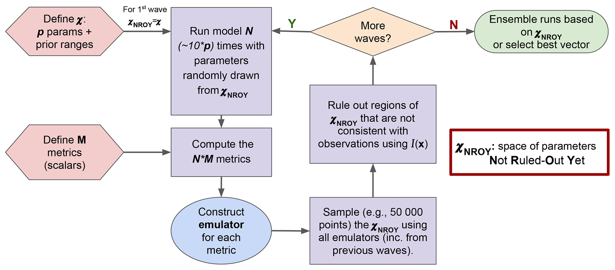
Figure 1 illustrates how HM is used in the ORCHIDAS system. We first define our p-dimensional parameter space 𝒳. From this space, parameter sets are randomly drawn and used to run the model. It is common to run the model for approximately 10 times the number of parameters (Loeppky et al., 2009). The outputs from each run are then mapped onto scalar values with a metric (e.g. root mean square deviation, RMSD). Emulators are constructed for each metric, and these are used to sample from 𝒳_NROY. This allows us to have a lot more points than model runs in the ruling-out step. The implausibility (Eq. 10) is used to rule out points to refine the 𝒳_NROY. More waves can then be conducted using this new space until we are satisfied with the remaining space. If the 𝒳_NROY is empty after a wave, then it means that we cannot match the observations given the current error tolerances. If the 𝒳_NROY no longer reduces between successive waves, then it might signify that the emulator variance is too high relative to the spread of the ensemble. As such, training the emulator with more runs may be necessary. It may also mean that the system has converged, and all remaining points are within the tolerance set. As a result, we may be able to reduce the cutoff (a). Although in this study we only focus on the same metrics throughout each HM experiment, there is the potential to change them as the waves progress.

2.3 Experimental setup

2.3.1 Twin experiment

We perform a twin experiment to compare the different approaches in a controlled manner. This means that we generate a set of pseudo-observations using a “true” set of parameters; here, we use the default ORCHIDEE values. Gaussian white noise, with a standard deviation set to 0.1 times the time series' mean, was added to each time step to represent the model/observation error. We use this error to set up the experiments, with e+η (with η=0) for HM and the diagonal element for the R in VarDA. We further use a diagonal B in our VarDA experiments, where the prior uncertainty is set to 100 % of the parameter range of variation (compared to 40 % of the range used in Kuppel et al., 2012) to allow for maximal space exploration.

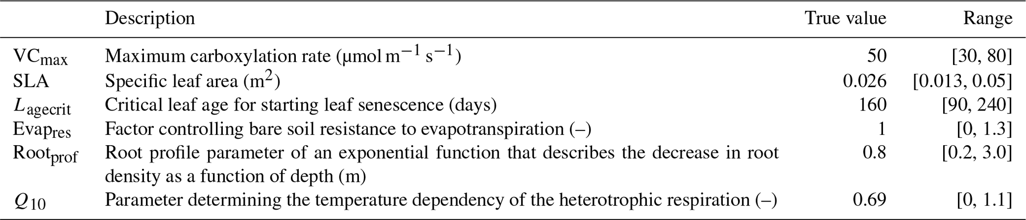
We focus our study on a temperate broadleaf deciduous forest site from the eddy covariance Fluxnet database (Pastorello et al., 2020), FR-Fon (Fontainebleau-Barbeau; Delpierre et al., 2016). This site is often used in our calibrations. Here, we focus on the first year of the time series (year 2005) for calibration (to save on computational cost) and the rest of the time series (years 2006–2009) for evaluation. Since we are running a twin experiment, and therefore, the observations are artificially generated, we only use the Fluxnet meteorological data to drive our model. As in previous work (e.g. Kuppel et al., 2012; Bastrikov et al., 2018), we focus on the model's ability to simulate net ecosystem exchange (NEE) and latent heat (LE) fluxes. NEE represents the difference between carbon dioxide uptake by plants through photosynthesis and carbon release through respiration, with the growing season typically being characterised by negative NEE that indicates net carbon absorption. LE represents the exchange of energy between the Earth's surface and the atmosphere through the phase changes in water, with higher values during periods of increased evaporation and transpiration often associated with warmer seasons. The parameters for this study were chosen with these fluxes in mind, using our past expertise, a preliminary Morris (1991) sensitivity analysis, and the desire to work with a small set of parameters (see the Supplement for more on the preliminary sensitivity tests). These parameters are listed in Table 1.

Table 1 ORCHIDEE parameters used in this study. True value refers to the default value of each parameter in ORCHIDEE. These values were used to generate the observations used in the twin experiment. Range refers to the range of variation allowed for each parameter.

2.3.2 Performed experiments

To minimise the cost function (Eq. 5) in the VarDA experiments, we consider both BFGS (local gradient descent) and GA (global random search) optimisation techniques. For BFGS, the algorithm is run for 25 iterations, which was found to be sufficient for the optimisation to converge. For GA, a population of 24 and a mutation rate of 0.2 were used, along with 25 iterations. These values are based on previous optimisations performed using Fluxnet data to optimise simulated NEE/LE in the ORCHIDEE model (Bastrikov et al., 2018) and were also found to be sufficient for convergence.

We perform two sets of experiments per minimisation algorithm. The first set of experiments uses B_post to assess posterior distributions after a single optimisation. To calculate the posterior uncertainties, we sample 10 000 points from 𝒩(x_opt,B_post) using the random.multivariate_normal function from the NumPy Python package (Papoulis, 1991; Duda et al., 2001). In the second set of experiments, we perform many optimisations (200), starting from random priors, and use the posterior parameter values to elicit the posterior parameter uncertainty. Given the probabilistic results obtained, we refer to these experiments as “stochastic”. In a standard optimisation, we would use the default model parameter values as the prior since they are our best guess. However, as we are performing a twin experiment in which the default parameter values are the true solution, we must start from a different part of the parameter space. To do this, we generate several random parameter sets. For the B_post experiments, where we consider only one optimisation, we chose the randomly generated parameter set that starts closest to the true values to be the most realistic. Although not shown, we repeated the analysis using a different prior, which gave similar results. For the stochastic experiments, we start from 200 different uniformly and randomly generated priors.

For HM, we do not need to worry about prior parameter values – only the parameter ranges. For each wave, the model is run 60 (i.e. 10 times the number of parameters) times. Initially, we consider the RMSD between the model and true model run as the target metric since this closely relates to the cost function used in VarDA (Eq. 5). In the second part of the study, we vary the metrics to fully explore the power of HM. Indeed, using RMSD is often discouraged since it is usually associated with a small signal-to-noise ratio. Furthermore, the implausibility (Eq. 10) is already similar to the root mean square error (Couvreux et al., 2021). In this section, we consider additional metrics to highlight the power of HM. To select informative metrics, it can be helpful to identify specific features that we want to constrain. For example, for both the NEE and LE fluxes, we are looking at a seasonal cycle. As such, we expect NEE to have a global sink (i.e. maximum carbon uptake) and LE to have a global peak (i.e. maximum evapotranspiration) in summer. As well as constraining the magnitude of these turning points, we might also want to consider constraining when they occur or the rate of change leading to and from them (i.e. the gradient of slopes). Evap_res and Root_prof parameters impact the slopes of the LE seasonal curve in spring and autumn, respectively, so focussing on these gradients may help better inform us about these parameters. Similarly, L_agecrit impacts senescence, so the slope in autumn is of particular interest. We also know that in winter, there will be little to no photosynthesis (since we are considering a deciduous site). Similarly, we expect low rates of terrestrial ecosystem respiration during these months and, therefore, can constrain NEE in winter. This is similar to constraining the initial carbon pools in the model. In this work, we consider four of these metrics: (i) min/max of the seasonal cycle (sink for NEE; peak for LE), (ii) the slope during spring (taken as the difference between April and February monthly means) and (iii) the slope during the senescence period (taken as the difference between September and August monthly means), and (iv) initial carbon stocks (NEE only). We perform five experiments, with four using different metrics (listed in Table 2) and the fifth combining all metrics. We perform 10 waves in each case and keep a constant cutoff of 3. At each step, we check the emulator quality (see Sect. B). We also retain the true model runs that are below the cutoff to train the next emulators.

Table 2 Target and variance used for each metric tested in the HM experiments. Min/max are taken as the minimum/maximum of the smoothed annual cycle (12-period rolling mean with a window size of 5). Spring slope is taken as the difference between April and February monthly means, autumn slope is taken to be the difference between September and August monthly means, and the initial C stocks are taken as the starting value of the time series.

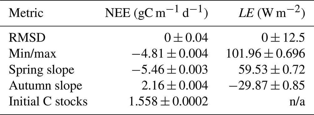
n/a – not applicable.

3 Results

3.1 Comparing variational data assimilation and history matching

3.1.1 Model–data fit

The first step in any calibration experiment is commonly to check the posterior model–data fit. Instead of considering the fit given by a single parameter set for each experiment, we consider the ensemble of posterior parameters taken from each experiment (Fig. 2). For the VarDA results, we consider model runs generated from each optimal parameter set found in the stochastic experiments (i.e. 200 optimisations) since these results give a larger posterior spread than the B_post experiments (not shown). For HM, we consider the experiment using the RMSD as the target metric since this most closely relates to the cost function used in VarDA. For consistency, we consider 200 parameter sets sampled from the 𝒳_NROY found at the end of the experiment (i.e. after 10 waves) and use these to run the model to create the posterior ensembles.

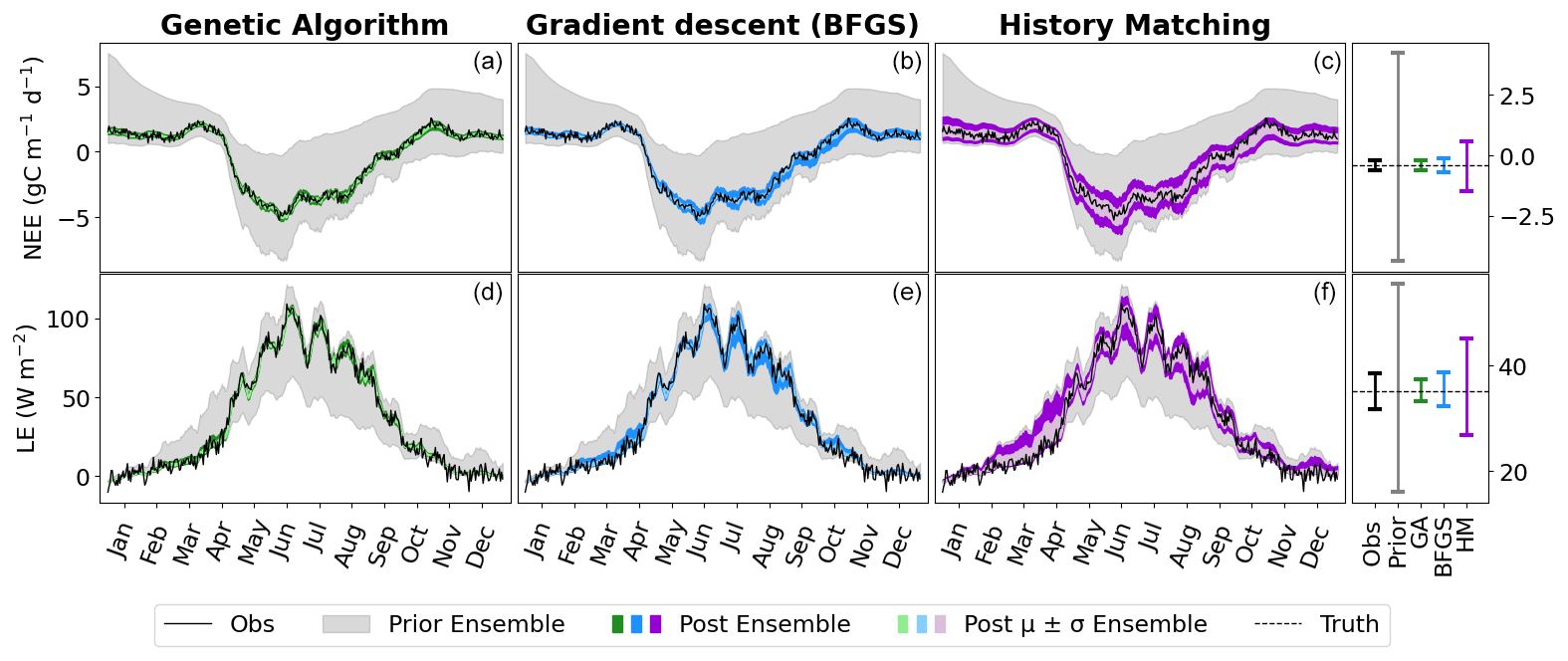
Figure 2 Time series of NEE (a, b, c) and LE (d, e, f) for FR-Fon year 2005. For the VarDA experiments (minimisation methods GA and gradient descent BFGS), the spread represents the results taken from the stochastic experiments (i.e. from 200 optimisations). For the HM experiment, 200 parameter sets were sampled from the 𝒳_NROY and used to run the model. The prior ensemble, i.e. before any calibration, is shown in grey, and the posterior ensemble is shown in dark colours. The lighter-coloured spread shows the mean and standard derivation of the posterior ensemble. The bar plots on the right-hand side show the range of the mean of each ensemble time series. Note the difference in scales.

The model–data fit in all experiments is much improved compared to the prior ensemble, with the GA experiment closely matching the observations, BFGS performing second best, and HM retaining the most spread. Overall, we are able to capture the seasonality and general magnitude of the observed fluxes. Typically, the only parts of the observations that are not contained in the posterior spread are the LE winter values, which are also outside of the prior ensemble spread. This suggests that these values are not reproducible by the model and represent the structural error (i.e. the noise we added to the true model realisation used to generate these pseudo-observations). We also note that the GA experiment gives an ensemble spread that is smaller than the spread of the noise on the observations, suggesting that these parameter sets may have overfitted the data.

Although the general shape of the seasonal pattern is reasonably well matched, we can see that there are parts of the time series that we are less able to constrain, especially with the HM experiment. This can be seen from the slope in spring, for example (also noticeable for BFGS), and the behaviour in summer. This highlights the issue of relying on a single metric in the optimisation process to capture the full behaviour of a time series, particularly the RMSD. The RMSD is prone to correcting large errors and therefore may be strongly driven by outliers. As such, it works well at correcting the errors in amplitude but less well at fitting other temporal features.

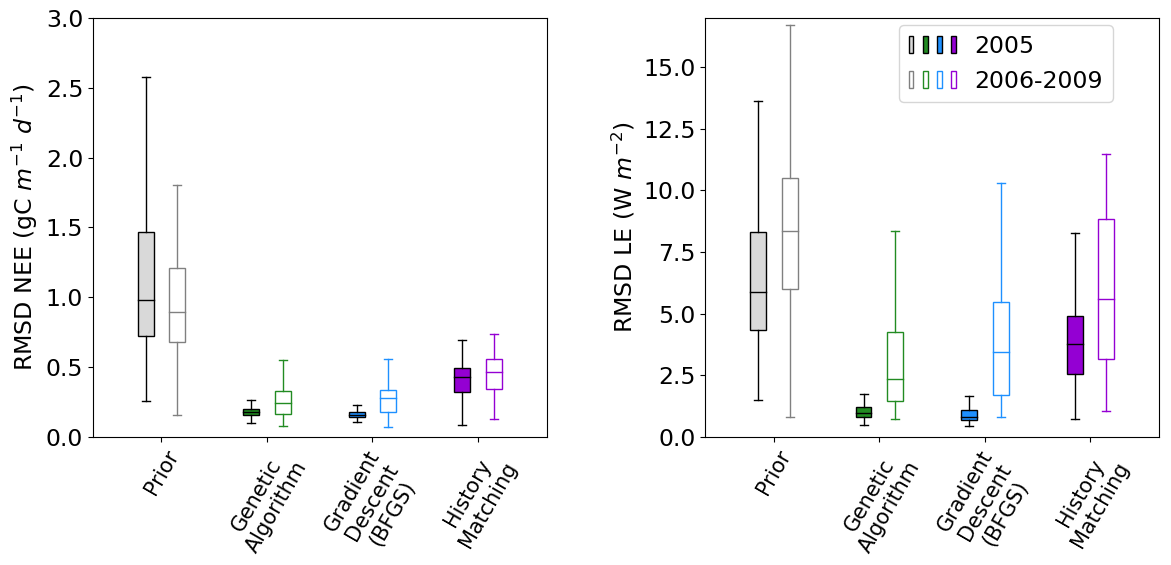
Figure 3 Boxplots showing the distribution characteristics of the RMSD of each of the 200 runs for the calibration year (2005; filled boxplots) and the evaluation years (2006–2009; outlined boxplots). The box represents the interquartile range and contains the central 50 % of the data. The horizontal line inside the box marks the median. Whiskers extend to the minimum and maximum values within 1.5 times the interquartile range. Full time series corresponding to these plots can be found in Fig. C1.

Figure 2 shows the fit to the calibration year – i.e. the one used to tune the model. We also tested the ensembles over several more years (2006–2009) to further evaluate the results. This evaluation step is important to check that we do not over-tune to the specificities of a given year but find parameter sets that work against the data not used in the calibration. We see that the ensemble spread is reduced for all methods and years (Fig. 3). This is most significant for the NEE, which started off with larger errors relative to the magnitude of the time series than LE. We see the largest reductions in the RMSD for the BFGS and GA minimisations in the calibration year, where the median of each boxplot reduces by over 80 %. When applied over the evaluation period, the reduction in RMSD is not as severe – especially when considering LE. For NEE, the resulting RMSD for the HM experiment is more consistent between the calibration and evaluation periods, suggesting that the more conservative approach has stopped us from overfitting to the calibration year. This consistency is less apparent for LE, but we do still see more overlap between the RMSD for the calibration and evaluation period for HM than the two minimisation methods.

3.1.2 Posterior parameter uncertainty

Variational data assimilation

In this next section, we take a closer look at the posterior parameter distributions themselves. As described in Sect. 2.2.2, after minimising the cost function in a VarDA experiment, we usually use information about the curvature of the parameter space to calculate the posterior covariance error matrix B_post (Eq. 6). Figure 4a shows results from the single GA and BFGS optimisation experiments (i.e. the optimisation with the randomly generated prior closest to the true values). For both optimisations, the reduction in parametric uncertainty is quite severe for all parameters, and for half of the parameters, the true value does not fall in the posterior distribution. The differences observed between the optimisations are mainly because we did not converge to the same x_post. The two most sensitive parameters (VC_max and Q₁₀) have the lowest posterior uncertainty. While still tightly constrained, SLA has the largest posterior uncertainty after both optimisations. After BFGS, Evap_res and Root_prof have a larger uncertainty than after the GA optimisation. This suggests that the minimum found from the GA optimisation is more constrained than the minimum found from the BFGS optimisation.

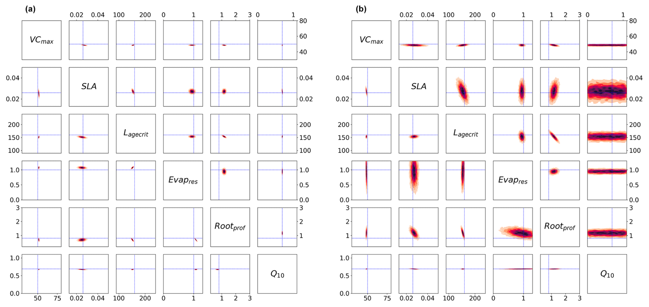
Figure 4 Posterior distributions obtained using B_post (Eq. 6) shown by kernel density estimation plots. Each sub-box is a 2D representation of parameter space showing the density for each pair of parameters, with darker regions signifying areas with higher data density. The true parameter values are shown in blue. (a) Full B_post for the GA optimisation (bottom triangle) and the BFGS optimisation (top triangle). (b) B_post decomposition (Eq. 8) for the BFGS optimisation with NEE (bottom triangle) and LE (top triangle).

In Fig. 4b, we consider the impact each of the two fluxes has on the parameter posterior distributions (following the decomposition in Eq. 8). Although the decomposition is shown for the BFGS optimisation, the GA optimisation gives similar results. The results show that the full posterior distribution of the different parameters is the intersection between the posterior distribution of each flux. This is most clearly illustrated by parameter Q₁₀. This parameter is highly constrained after the optimisation for NEE flux. In contrast, this parameter does not impact the modelled LE and, therefore, is not constrained by this flux. As such, Q₁₀ can take any value for this LE, and so the distribution spans the whole range. Therefore, when accounting for both fluxes, the posterior distribution for Q₁₀ matches the NEE constraint. We can further interpret the information in Fig. 4b as the flux sensitivity to each parameter, with constrained parameters being the most sensitive and unconstrained the least sensitive. From this we see that in addition to Q₁₀, NEE is more sensitive to SLA than LE and to L_agecrit, although to a lesser extent. LE is more sensitive to Evap_res. Both fluxes give similar constraints on Root_prof. These results are consistent with our understanding of the model and the impacts of the different parameters.

Although this decomposition is very informative, it does not explain why the true values do not always fall within the total posterior distribution. There are several reasons why this might be the case, including the two key assumptions made when calculating B_post. First, we assume that we have found the global minimum, and second, we assume the linearity of the model in the vicinity of the solution, resulting in a Gaussian posterior distribution. This means the B_post method is unable to take into account any non-Gaussian uncertainty.

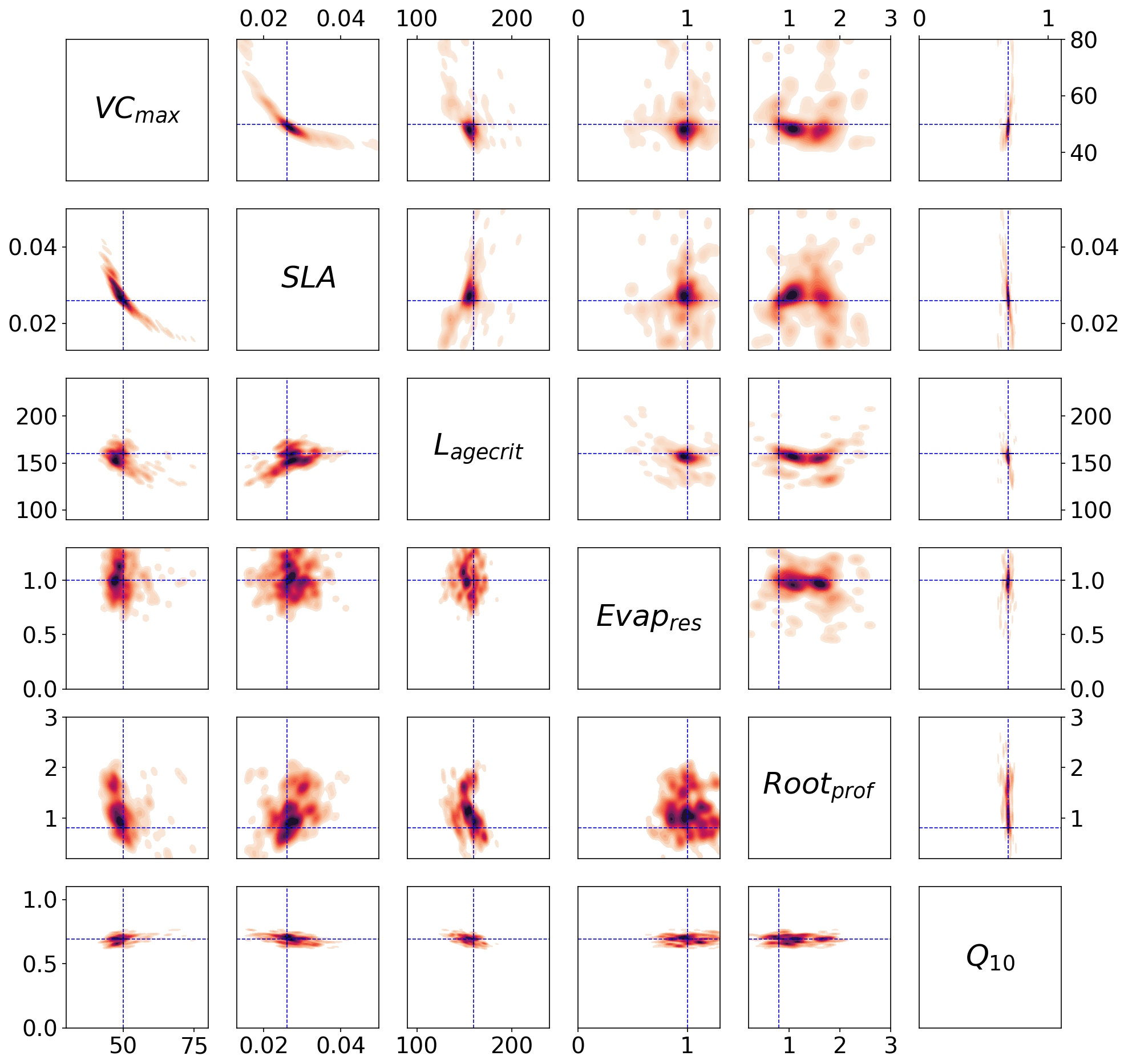
Figure 5 Posterior distributions obtained from the stochastic experiment shown by kernel density estimation plots. Each sub-box is a 2D representation of the parameter space showing the distribution of the 200 different x_post found with GA (bottom) and BFGS (top), with darker regions signifying areas with higher data density. The true values are shown in blue.

We can use the stochastic experiments to bypass these assumptions. Unlike the B_post method, we no longer have a Gaussian assumption on the posterior uncertainty, allowing us to find non-Gaussian distributions. Furthermore, we have an ensemble of posterior parameters, so the assumption of being at the global minimum is less important. Figure 5 shows the x_post ensemble obtained after 200 optimisations using both minimisation techniques. We see immediately that allowing for a non-Gaussian posterior distribution reveals more information about the parameters. For example, a clear relationship between VC_max and SLA is found by both minimisation techniques. There is a trade-off between the two parameters – if the leaf has a small surface area (SLA), then the leaf's capacity to capture carbon (through VC_max) is increased. We further obtain a two-peaked posterior distribution for Root_prof (clearest in the BFGS experiment). This parameter defines the depth above which ∼65 % of roots are stored. The double peak suggests that either most of the roots are stored above 1.5 m, and the trees will primarily get water from the subsurface, or the roots grow deeper to access water down the soil column. Both options would result in the trees having the same water availability. For Evap_resp, both minimisation techniques remove the possibility of low values, and for L_agecrit, the posterior distribution is centred on the range. We again see that Q₁₀ is the most constrained parameter relative to the prior range.

Unlike the B_post experiments, here the true values are contained within the posterior distributions (see Fig. C2 for 1D distributions). The distribution of solutions is similar for BFGS and GA. Nevertheless, the GA distributions are slightly tighter and more dense. This is because GA is a global search algorithm and, therefore, less likely to get stuck in local minima. The fact that we still get a large variation in solutions, while still obtaining a similar fit to the model in Fig. 2, further highlights our problem of equifinality.

History matching

To directly compare HM to the VarDA approach, in Fig. 6 we use the RMSD between the observations and the model output for both NEE and LE as metrics. Already in the first wave the 𝒳_NROY reduces by over 80 % (Table B1). This is further reduced to less than 10 % of the original parameter space by the end of the 10th wave. Furthermore, the true parameter values exist in 𝒳_NROY. We can also see some of the same patterns we were starting to observe in Figs. 4 and 5. Most notable is the relationship between VC_max and SLA and the strong constraint on Q₁₀, where values below 0.45 of this parameter are ruled out. Similarly, values of L_agecrit below 124 are ruled out. In contrast, Evap_res and Root_prof are not constrained at all by this experiment; there is not enough information to rule out any values. These two parameters impact LE, specifically its slope, in spring and autumn.

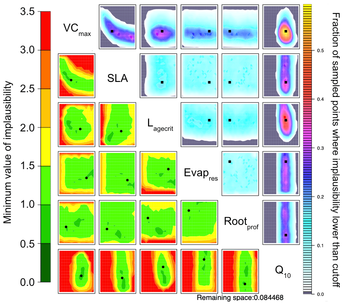
Figure 6 NROY density plots (upper triangle) and minimum implausibility plots (lower triangle) from the HM experiment using NEE and LE RMSD as metrics after 10 waves. NROY densities (or optical depth) represent the fraction of points with implausibility smaller than the cutoff a (here a value of three) using the colour bar on the right, with grey regions indicating completely ruled-out areas. This fraction is obtained by fixing the two parameters given on the main diagonal at values of the x axis and y axis of the plotted location and searching the other dimensions of the parameter space. Minimum implausibilities represent the smallest implausibilities found when all the parameters are varied, except those used as x and y axes. These plots are oriented the same way as those on the upper triangle to ease visual comparison. True parameter values are shown in black, with the square on the NROY density plots and circle on the minimum implausibility plots.

3.1.3 Computational cost

The computational cost of calibration algorithms is primarily determined by the number of parameters and the time it takes to perform a single model run. In this study, we test the different methods over a single pixel for a single year, which only takes seconds to run, meaning the ensembles needed for each algorithm were not too costly to generate. However, in practice, a single model run can be costly – especially when running the model over a large area or coupled with an atmospheric transport model. Table 3 shows the number of simulations needed for each algorithm. Note that the extra computation time needed to construct the emulators and use these to sample from the NROY space is marginal in comparison.

Table 3 Number of model runs needed in each algorithm for p parameters. Note that the BFGS and GA algorithms were run 200 times for the stochastic experiments.

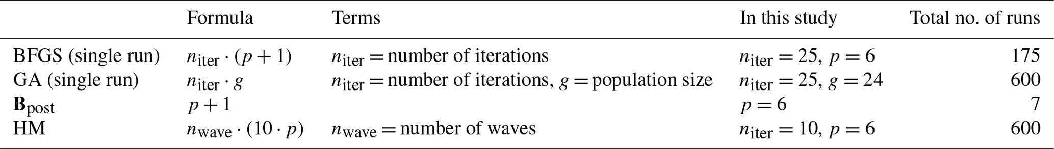
These values represent ballpark figures – a maximum iteration of 25 was used for consistency, but the system often converged sooner (e.g. approximately 10 iterations for each BFGS run). Similarly, we used 10 waves for HM, but after the fifth wave, the improvements were marginal (Table B1). Overall, a single BFGS optimisation (i.e. gradient descent) remains the fastest method. However, it is also the one that is most likely to get stuck in local minima. HM is comparable to a single GA run in terms of the number of simulations needed. However, we have seen that a single GA run is not enough in this example to quantify the posterior parameter space fully. Instead, multiple GA optimisations are preferable (here we used 200), which is extremely costly.

3.2 Implementing process-oriented metrics

One of the strengths of HM is that we can easily apply different metrics, and so in this section, we consider the additional constraints that these metrics bring. In Fig. 7a, we consider how the minimum/maximum of the seasonal cycle can be used to constrain the parameters. We again highlight the VC_max–SLA relationship. Another relationship found is between VC_max and Root_prof. Although this metric cannot be used to rule out unlikely values of Root_prof, there is a denser fraction of likely points falling around 2.3. Note that this is not the true value of the parameter but is closer to the value of the second minimum found in the stochastic experiments. When considering VC_max, VC_max is constrained to 50 when Root_prof is small. However, when Root_prof is large, i.e. the roots can access water further down the soil column, VC_max is less constrained. This means that when there is more water availability, the carbon capture capacity of the plant is less important in determining the peak and sink of the NEE and LE seasonal cycles, respectively. Although 35 % of the parameter space is left, we see clearly that this metric is insufficient to constrain the other parameters. Indeed, the minimum/maximum is not sensitive to L_agecrit, Evap_res, and Q₁₀. When considering the time series for this experiment, the fit is not too dissimilar from Fig. 2 when using the RMSD as the metric. However, we see here that winter behaviour is not constrained. This is especially true for the NEE time series; we do not reduce the spread at the beginning and end of the year.

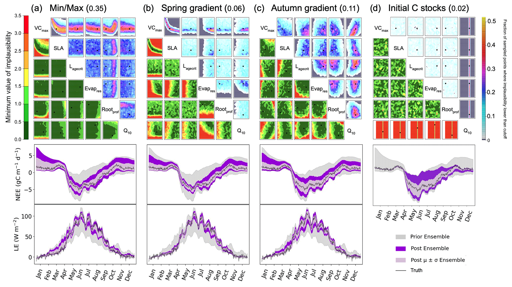
Figure 7 History-matching experiments considering different individual metrics. NROY density plots are shown above (see Fig. 6 for how to interpret the figure) with the proportion of the remaining space after 10 waves in the title parentheses. The time series plots shown below each density plot illustrate the ensemble spread generated when running the model with 200 parameter sets sampled from each 𝒳_NROY.

Figure 7b and c use the slope in spring and autumn, respectively. For the spring slope metric, we again pick out the relationship between VC_max and SLA. This is even sharper than in the RMSD and the minimum/maximum cases. We also notice a relationship between Evap_res and Q₁₀, with values in the lower left-hand corner of the space ruled out. Similarly, low values of Evap_res are ruled out using this metric. When considering the time series, we clearly reduce the spread of the ensemble in spring for the LE. We also reduce for NEE; however, this is less obvious since the prior ensemble spread was already quite narrow. For the autumn metric, we start to constrain L_agecrit and Root_prof and SLA to a lesser extent. These are parameters that we did not constrain using the other metrics tested. Changes to the ensemble spread in the time series are similar to when the RMSD was used as the metric, although a little more marked during September of the LE time series.

The final metric considered in Fig. 7d considers constraining the initial carbon stocks. We clearly see that this metric is completely controlled by a single parameter, Q₁₀. This parameter has been the most constrained throughout, and here we see why. It directly impacts the spread of NEE at the beginning and end of the time series. For the rest of the time series, this parameter has no impact – the ensemble spread in summer is at its maximum width.

These examples illustrate clearly how we can use individual metrics to target different parts of the seasonal cycle. The next step is to combine them in one experiment. In Fig. 8, we combine these five metrics (RMSD, min/max, spring slope, autumn slope, and initial carbon stocks) to have a total of nine constraints (each of the metrics is applied to both NEE and LE, except for the initial carbon stock metric which is only applied to NEE; see Table 2). Note that these metrics are not weighted (in the traditional sense) when combined. Instead, the weighting occurs through the individual errors used to set up the experiment.

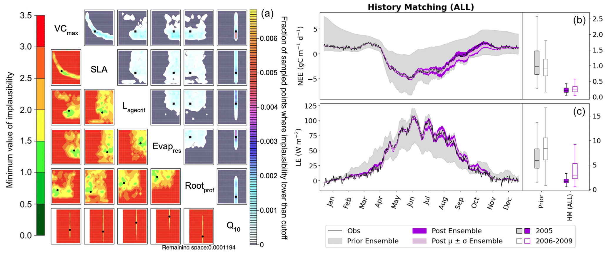
Figure 8 History-matching experiment considering all metrics listed in Table 2. Results from the third wave are shown with the NROY density plot on the left (see Fig. 6 for how to interpret the figure). The time series shown on the right depicts the spread of 200 ensemble runs generated from points sampled from the 𝒳_NROY (shown in dark purple), with the mean and standard derivation of this spread shown in light purple. The boxplots in panels (b) and (c) show the distribution characteristics of the RMSD of each of the 200 runs for the calibration year (2005; filled boxplot) and the evaluation years (2006–2009; outlined boxplot).

Using these multiple metrics, the 𝒳_NROY is reduced to 0.01 % of its original size. We see that all of the parameters are constrained with the true points still contained in the NROY space. Indeed, the true values lie in the space where the minimum implausibility is at most 1.5. We would still recover these points if the cutoff were decreased from its current value of three. The relationship between VC_max and SLA is kept, and we can pick out the true value of Q₁₀. By comparing to Fig. 6, we can see that combining different metrics has helped reduce the space to a much greater extent by constraining the other parameters that were not constrained by solely relying on the RMSD. When considering the time series, we see that the posterior ensemble of model runs tightly fits the observations – especially at the beginning of the year. The ensemble spread is more reduced than when we only used the RMSD (Fig. 2) but with the same consistency between the calibration year and the rest of the time series, especially for NEE.

Using these physical metrics and targeting different parts of the seasonal cycle, we are able to better fit the data and gain an understanding about the parameters. We still have some variability in late autumn, with the model runs tending to underestimate NEE. Currently, we only target the slope between the September and August monthly means to capture the leaf senescence. If we further included a metric in October or November, we may be able to constrain the time series further. Ideally, this would be based on some physical process to understand which parameters would be the most impacted. We also expect that targeting the variability in the summer months would help constrain LE during July and August. This would most likely target Root_prof and Evap_res, as variability during these drier months will impact the amount of water in the soil.

4 Discussion

This study provides a good introduction to how HM can constrain the carbon and water cycles in land surface models. Nevertheless, it is not without limitations. In the first part of the study, we compare it to VarDA, which is often used for parameter estimation in land surface models (especially when calibrating the ORCHIDEE land surface model), and consider two different minimisation algorithms to reduce the cost function. However, properly comparing VarDA and HM is hard since they are both designed with different goals. This means that discussions around computational cost are nuanced – there are no comparable convergence criteria. Furthermore, for each algorithm, there is a trade-off in computational time and efficiency. For example, we can use more model runs to fit emulators in HM or increase the population size in GA.

In this study, we use gradient descent BFGS and random-search GA to find the optimum and then the gradient information at the optimum to find the posterior uncertainty (through B_post; Eq. 6). We do acknowledge that there are other methods we can use to minimise the cost function – ones where the ensembles can be used to infer the posterior distributions (e.g. Markov Chain Monte Carlo; Geyer, 1992). However, these are extremely costly and therefore outside the scope of this study. Furthermore, we wanted to use the method currently used in ORCHIDAS and, therefore, where we have the most understanding and experience. Finally, whilst we do not expect it to have a huge impact on the results, without the adjoint of the ORCHIDEE model, B_post only approximates the curvature of the parameter space, and therefore, the posterior parameter distributions found with this matrix are not accurate. Maintaining the adjoint of a complex model like ORCHIDEE is very costly, given the model's evolving nature. Therefore, the fact that HM does not need the adjoint in its calculation of posterior distributions is an advantage.

In the second part of the study, we look at using different metrics for training emulators to use in HM. Although using different metrics is also possible in VarDA, this is trickier since the choices must be made before a costly calibration (for example, which metrics to use and how to weight them). With HM, we can run an ensemble first and test different metrics on the ensemble. Adding new metrics as the waves progress is also possible instead of restarting the whole optimisation procedure. In this study, we chose a few illustrative metrics based on our understanding of the physical processes driving the model and the results of the one-at-a-time sensitivity analysis (Fig. A1 in Appendix A). Choosing the best, most suitable metrics could be the subject of a whole separate study. Furthermore, increasing the objectivity of the tuning procedure will allow the climate modelling community to more meaningfully share insights and expertise with each other, thereby increasing our understanding of the integrated climate system. In addition to performance-based metrics (e.g. RMSD and skill scores), physically based metrics allow us to target different parts of the model. However, these require an understanding of the different processes involved. While here we focused specifically on parts of the seasonal cycle, there may be other more complex metrics to consider (for example, the timing of the leaf area index reaching a certain threshold). Furthermore, we can use techniques such as a principal component analysis to help reduce the dimensionality of the problem (Lguensat et al., 2023).

Nevertheless, HM does come with its own challenges. It is, in a way, much more involved and requires a level of understanding to ensure the emulators are properly constructed and applied. There are also a number of subjective choices that can be made during an HM experiment, such as changing the cutoff (a in Eq. 11) if the emulator is believed to be good enough, which requires some level of understanding beyond using the method as a black box. When combining a large number of the metrics, it is also possible to expand Eq. (11) to allow for some additional flexibility (Couvreux et al., 2021). For different metrics m_i, 𝒳_NROY is the intersection of the ${\mathcal{X}}_{{\mathrm{NROY}}_{m_i}}$ associated with each metric,

$$\begin{array}{}\text{(13)}& \begin{array}{rl}{\mathcal{X}}_{\mathrm{NROY}}& =\bigcap _i{\mathcal{X}}_{{\mathrm{NROY}}_{m_i}}\\ & =\mathit{\{}\mathit{x}\in \mathcal{X}:\mathit{\#}\mathit{\{}\mathit{x}\in \mathcal{X}:{\mathcal{I}}_{m_i}\left(\mathit{x}\right)>a\mathit{\}}\le \mathit{\tau }\mathit{\}},\end{array}\end{array}$$

where # denotes the number of metrics that satisfies the condition in the bracket, and τ is the number of metrics for which the model is allowed to be far away from the target. Throughout, we set τ=0, meaning that each model run must satisfy all the metrics. However, when combining many metrics, this value can be increased to stop us from accidentally ruling out good runs before the emulators are properly trained. Although not necessary in our test case, this τ can be an important consideration.

The example we test here is simple but illustrative. Nevertheless, we only test one site, and as we have seen, this suffers from a high degree of equifinality. Several studies have shown that moving from a single-site setup to multisite optimisations (i.e. finding one common set of parameters for multiple sites) results in a more robust optimisation that is less likely to get stuck in local minima (Kuppel et al., 2012; Raoult et al., 2016; Bastrikov et al., 2018). This is because the multiple constraints from the different sites smooth out parameter space. Even so, multisite optimisation can suffer from wider parameter uncertainty distributions as there are dynamics at various sites that are not explicitly included in the models, thus necessitating a robust preselection of the subset of sites used in the experiment. To further test the strength of the HM method, a new step will be to move to multisite setup. We anticipate that one of the strengths of HM, its use of emulators, will become more apparent when we move to these more costly experiments. Furthermore, emulators will greatly benefit the optimisation of larger regions and more costly processes (e.g. spin-up). Finally, although the twin experiment is very informative, a next key step will be to use real-world data to assess the full potential of HM.

4.1 Future avenues

HM is a promising approach that may prove invaluable in future land surface model calibration. One of the key challenges in land surface model calibration is multi-data stream optimisations. Ideally, we would perform simultaneous calibrations in which all the information is ingested in one go. However, this is not always practical. There may be some technical constraints like, for example, computational capabilities. We may also want to assimilate a newly acquired data stream without redoing the whole calibration process. The alternative is to perform calibrations in a stepwise manner by treating the data sequentially. If dealt with properly, the stepwise approach is mathematically equivalent to the simultaneous one (MacBean et al., 2016; Peylin et al., 2016). However, this means propagating the full parameter error covariance matrix between each step, which can be hard to estimate properly. This is where HM becomes particularly attractive. The NROY space contains all the information about the parameter errors, so this information is not lost between steps. Furthermore, HM's iterative nature means we can add different data when and as they become available. It also lends itself well to a stepwise approach to calibration, allowing us to separately constrain, for example, the fast and slow processes of the model. Finally, HM's conservative nature means that we are less likely to overfit to a particular data stream or indeed the particularities of given experiments, as shown here.

Although HM does not provide an optimal set of parameters at the end, this is not necessarily an issue. As computers become more powerful, we can run land surface models as ensembles instead of a single realisation of the model, allowing us to rigorously obtain the uncertainty in the model prediction. Indeed, as a climate community, we should be moving towards using data-constrained ensembles instead of a single realisation (Hourdin et al., 2023). HM would allow us to generate such ensembles to be used as, for example, the Coupled Model Intercomparison Project. Alternatively, we could use HM for pre-calibration (Edwards et al., 2011), i.e. reducing the parameter space before performing data assimilation. The 𝒳_NROY could further help us define the off-diagonal elements of the B matrix in Eq. (5). We also note that one wave of history matching is as costly as a Morris sensitivity analysis commonly used to assess parameter importance (Appendix A) but much more informative.

The true strength of HM is its ability to help with the identification of structural errors (Couvreux et al., 2021). Although we can also use VarDA to identify structural errors, HM's more conservative approach to parameter rejection can more easily help identify when the model is clearly wrong. Furthermore, once an ensemble is generated, applying different metrics to test different model sensitivities is easy (instead of performing a full optimisation, as would be needed in VarDA). It is common to add model complexity to models to address structural changes without first checking that the errors truly represent structural deficiencies and are not simply an artefact of poor model tuning (Williamson et al., 2015). Through HM, we can easily test for structural errors and see whether it is possible to match observations given the current model structure.

5 Conclusions

Using a twin experiment (i.e. with known posterior parameter values), we first compared the posterior parameter distributions found after variational data assimilation (VarDA) experiments to those found after a history-matching (HM) experiment. We found that the Gaussian hypothesis used to calculate the posterior uncertainty after the VarDA experiments was too strong. The posterior parameter distributions did not reflect the full equifinality of the parameter space or the non-linear behaviours and relationships of the different parameters. Furthermore, the true parameter values were not contained in the posterior distribution for half of the parameters. When performing multiple cost function minimisations starting from 200 different random priors, we achieved a better exploration of the parameter space. These experiments were much more computationally costly but started to reveal relationships between the parameters and contained the true parameter values in the posterior distribution. Similarly, while not constraining all of the parameters, the posterior distributions from the HM experiment also contained the true parameters and maintained non-linear relationships between the parameters. Furthermore, the model ensemble found by sampling the not-ruled-out-yet space fitted the observed time series reasonably well.

In the first part, we used the root mean squared difference as the target metric for HM to directly compare to the cost function used in the VarDA experiments. In the second part, we showed HM's versatility in using different metrics to target different parts of the seasonal cycle. This allowed for all of the parameters to be better constrained and the posterior model ensemble to tightly fit the observations. We showed that instead of using a single cost function, multiple process-based metrics improved the calibration and enhanced our understanding of the model processes.

Although this paper only considers a simple exploration of the HM methodology, its strong potential for land surface model calibration is clear. It will allow us to constrain multiple data streams, better targeting individual processes. Overall reductions in parameter uncertainty will lead to more accurate projections of the land surface, enhancing our understanding of terrestrial behaviour under climate change and allowing us to better plan for the future.

Appendix A: Parameter sensitivities

One of the primary uses of HM is to test the sensitivity of the model outputs to the parameter uncertainty. Nevertheless, we ran a couple of simple tests in advance to get a sense of the different parameter sensitivities. These more closely resemble the tests that land surface modellers perform when doing simple manual tuning and are not as rigorous as HM. However, they remain common – especially since they can be used to pre-select the key parameters for these more robust but costly methods.

The first is a simple, one-factor-at-a-time parameter perturbation experiment (Fig. A1). Although this does not account for interactions between parameters, it can help understand some of the direct impacts of the different parameters. This cost of the method is determined by the number of ensembles used for each parameter (here 50). The second is a Morris sensitivity analysis (Morris, 1991; Campolongo et al., 2007) (Fig. A2), which is effective with relatively few model runs compared to other more sophisticated methods (e.g. Sobol, 2001). Indeed, a standard Morris experiment equates to the computational cost of doing one HM wave (i.e. 10 times the number of parameter forward runs of the model). Using an ensemble of parameter values, the Morris method determines incremental ratios known as “elementary effects”. These effects are determined by sequentially modifying individual parameters across multiple trajectories within the parameter space. The mean (μ) and standard deviation (σ) of the differences in model outputs for all the trajectories are calculated. This global method determines which parameters have a negligible impact on the model and which have linear and non-linear effects. The results of this method are qualitative and serve to rank the parameters by their significance. To evaluate the results, we consider the normalised means, obtained by dividing each value by the μ of the most sensitive parameter. As such, the values fall within the range of 0 and 1, with 1 indicating the most sensitive parameters and 0 indicating parameters with no sensitivity.

Both methods clearly show that NEE and LE are highly sensitive to VC_max and SLA. In Fig. A1, we see that these parameters directly impact the amplitude of the seasonal cycle. NEE is most sensitive to Q₁₀ (the parameter determining the temperature dependence of heterotrophic respiration), which we see impacts the respiration (TER) component of this flux. This parameter has no impact on LE. After VC_max and SLA, LE is most sensitive to Evap_res, which controls bare soil resistance to evapotranspiration. This parameter impacts the slope in spring, controlling how much water is in the soil before the leaves start to grow at this deciduous site. Both fluxes are sensitive to L_agecrit in autumn, so this parameter impacts the age of leaves and therefore senescence. Finally, while still showing some sensitivity, the fluxes are least sensitive to Root_prof. This parameter controls root depth and seems to have the most impact in summer when the months will be warmer.

While the one-factor-at-a-time experiment seems more informative here, we must remember that it does not account for the interactions between the parameters. This can be dangerous because it is possible that changing different combinations of the parameters may impact the processes differently. This will be crucial in more complex cases. While the Morris experiment does account for interactions, it is not possible to disassociate from non-linear effects. Furthermore, although Morris is less costly, little information beyond simple rankings can be gleaned.

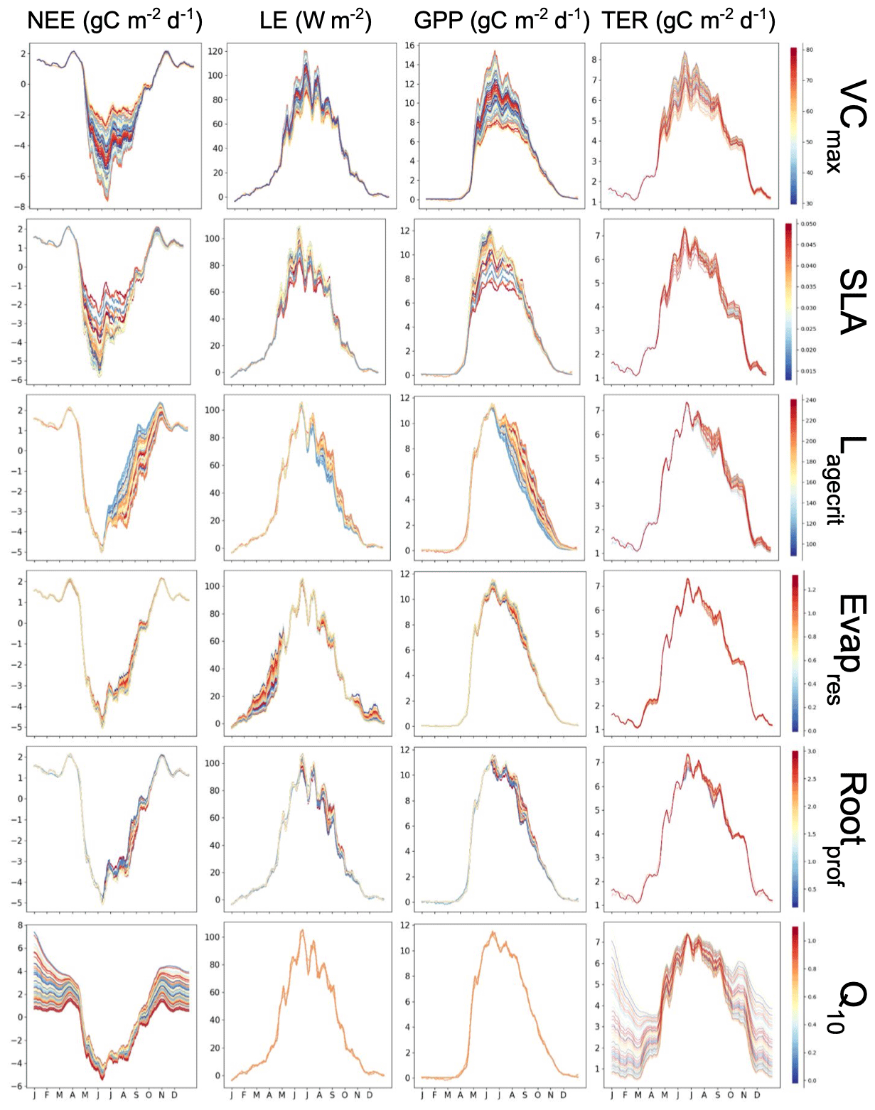
Figure A1 Preliminary experiment demonstrating the individual sensitivity of each parameter. For each row, 50 ensembles of a given parameter are shown for NEE and LE, as well as NEE's components of the gross primary production (GPP) and terrestrial ecosystem respiration (TER). Runs are coloured by the parameter values used, with low values in blue, passing through yellow, and high values in red.

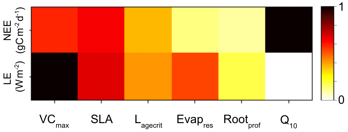
Figure A2 Heatmap showing the relative sensitivity of each parameter for NEE (top row) and LE (bottom row). Morris scores are normalised by the highest-ranking parameter in each case. Dark squares represent the most sensitive parameters for each output, and light squares represent parameters with little to no sensitivity.

Appendix B: Emulator quality

We ran leave-one-out cross-validations to validate the emulators at each wave of the HM procedure. Each point from the design set was retained for validation, and the emulator was refitted. We then test if that point lies within the 95 % confidence interval of the refitted emulator – if 95 % ratio of the left-out points should lie inside the confidence intervals, then the emulator is deemed good. While it is an ideal case, we consider in this work that the emulator is good if the ratio is at least over 90 %.

To illustrate this, Fig. B1 shows the diagnostic plots for the first and last wave of the HM RMSD experiment, and Table B1 shows the leave-one-out diagnostics at each wave. The emulator represents the model well for both the NEE and LE cases with small error bars and predictions close to true values. We obtain larger error bars for NEE compared to LE (especially in later waves) due to the more sophisticated behaviour of the model for the NEE case. In Table B1, we see that both the average error and variance decrease with successive waves, showing our emulators are becoming more accurate, and in each case, the accuracy is above the 90 % mark. Overall, we are satisfied with the quality of our emulators. Although not shown, emulators from the other HM experiments give similar results.

Table B1 Information about emulators and the leave-one-out diagnostics at each successive wave. The error column shows the mean emulator error, and the SD column shows the mean emulator SD for each prediction.

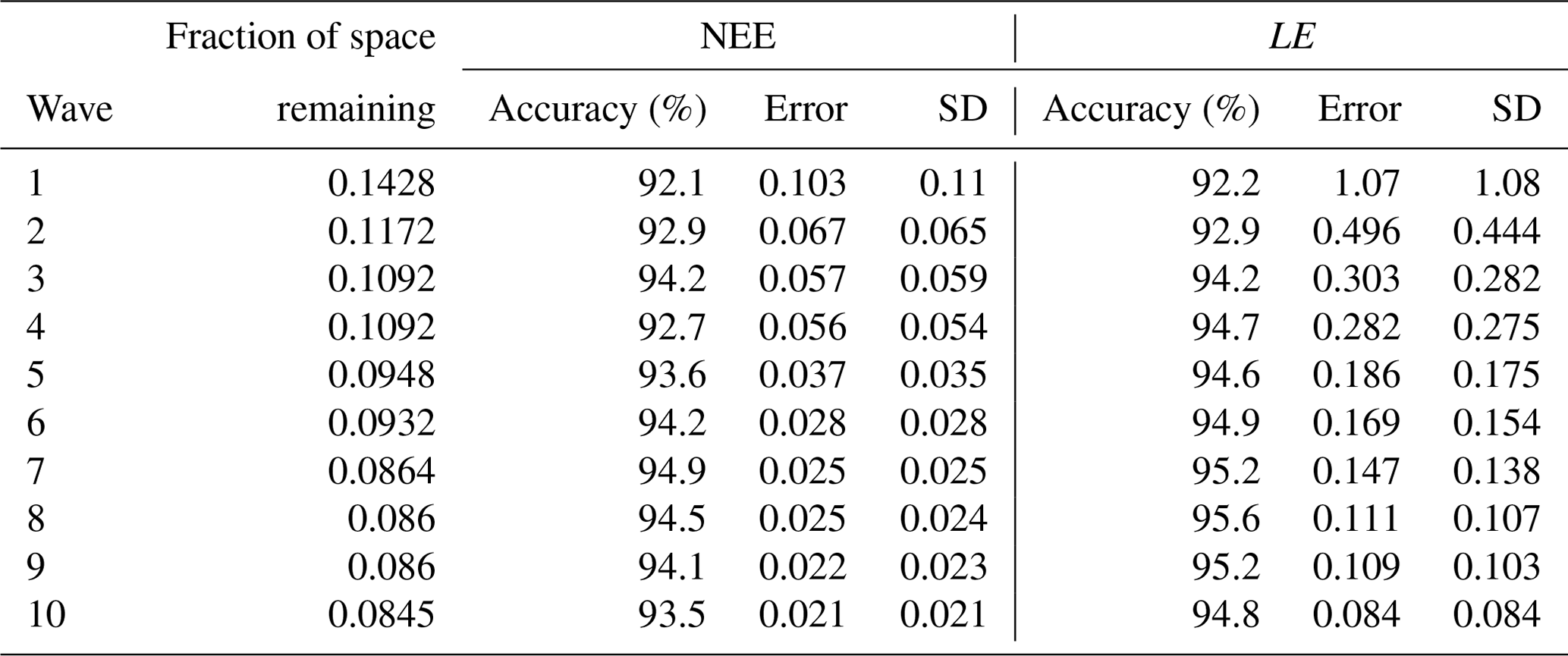
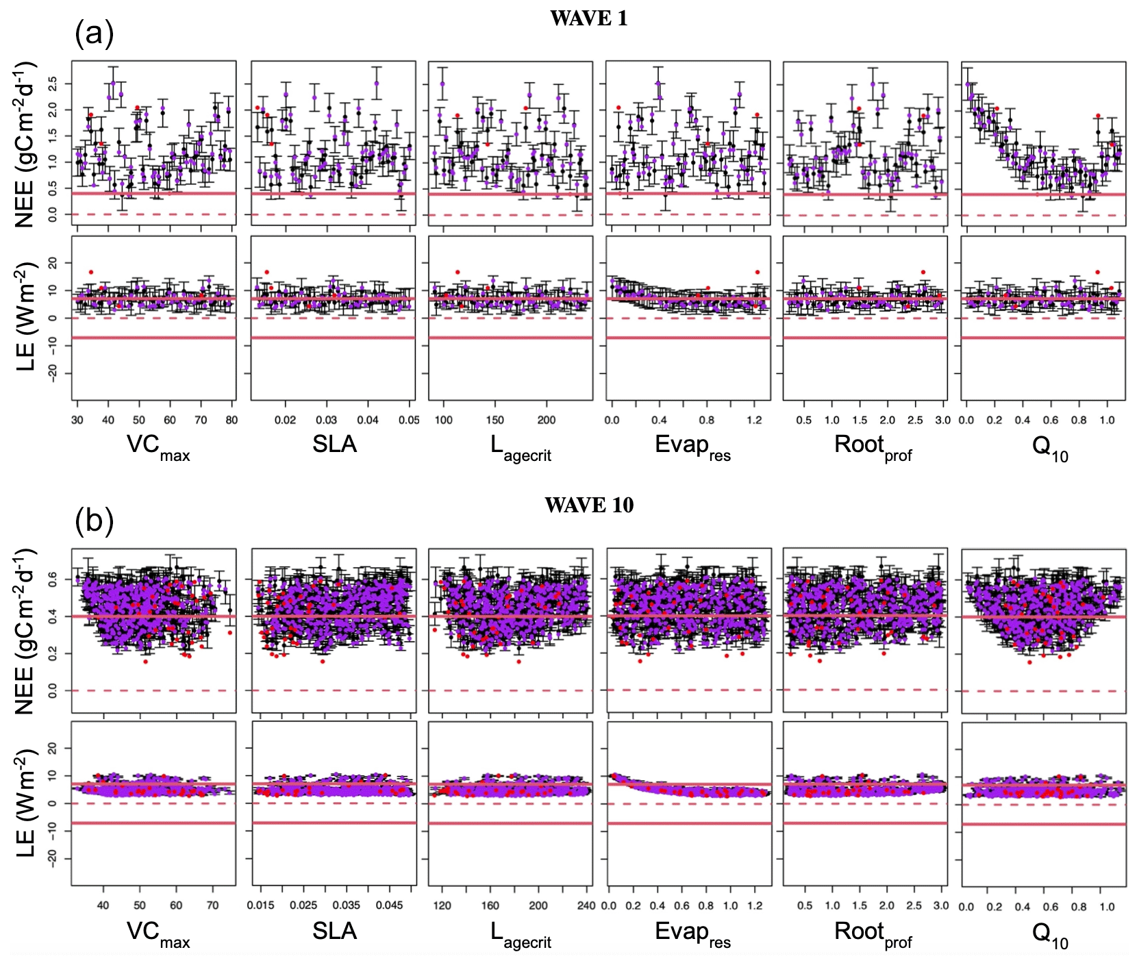
Figure B1 Leave-one-out diagnostic plots against each of the parameters for NEE (top row) and LE (bottom row) for the first and last wave of the history-matching RMSD experiment. Black points and error bars (±2 SD prediction intervals) are computed from E[H(x)] and Var[H(x)]. The true (left-out) values are plotted in purple/red if they lie within/outside 2 standard deviation prediction intervals. The horizontal dashed lines show the observations plus the observed error ($\mathrm{0}\pm \mathrm{2}\sqrt{\mathrm{Var}\left(\mathit{e}\right)}$). Note the difference in scale between the plots in wave 1 and wave 10.

Appendix C: Additional figures

Here, we present a few additional figures to help further visualise the results. Figure C1 shows the time series for the additional evaluation years (2006–2009).

Figure C2 compares the 1-dimensional posterior distributions found by the VarDA stochastic experiments and HM experiments. Remember that this is a 1D representation of multidimensional space and so does not illustrate the relationships between parameters.

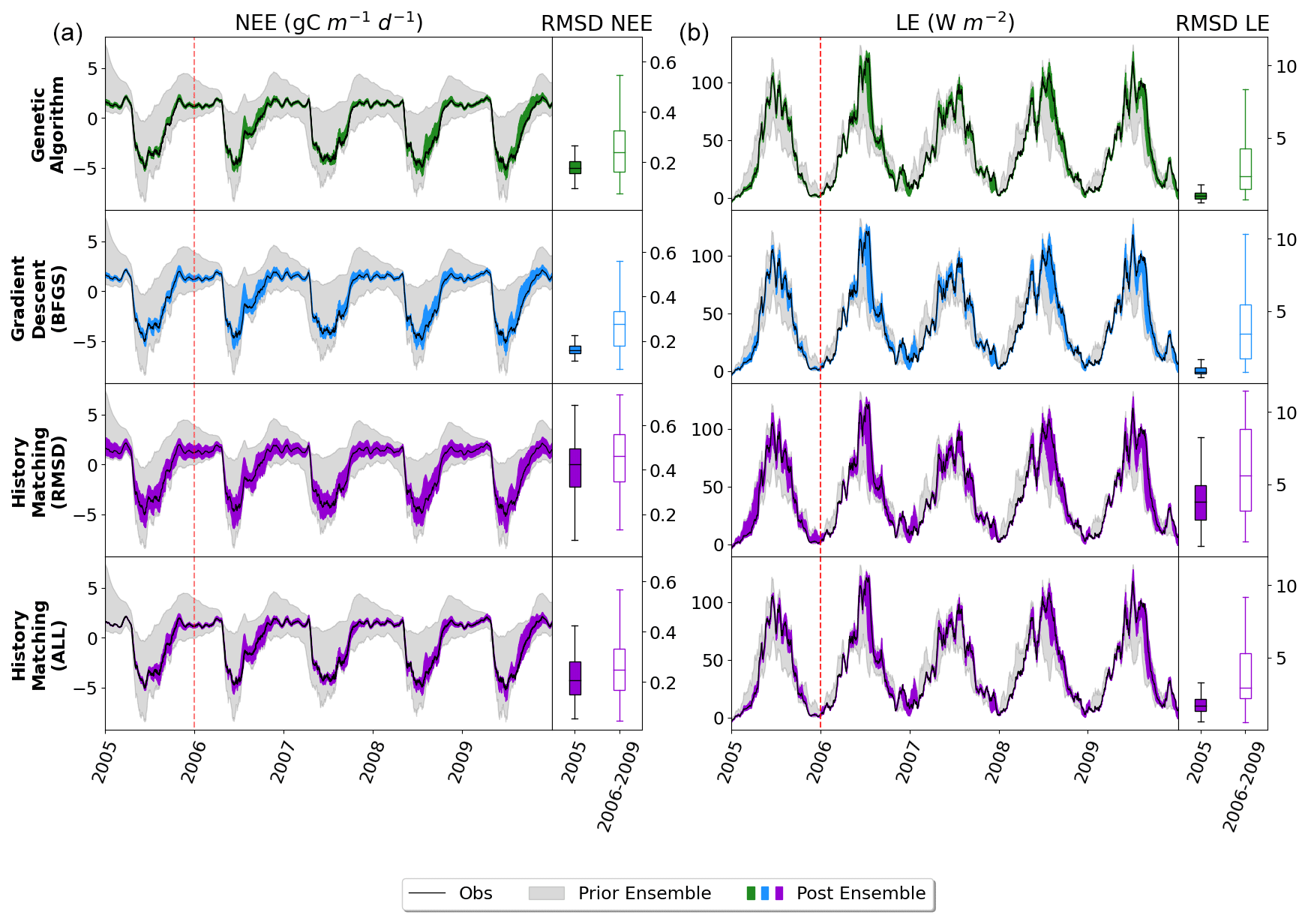
Figure C1 Full time series of NEE (a) and LE (b) for FR-Fon years 2006–2009. For the data assimilation experiments (GA and BFGS), the spread represents the results taken from the stochastic experiments (i.e. from 200 optimisations). For the HM, 200 parameter sets were sampled from the 𝒳_NROY and used to run the model. The prior ensemble, i.e. before any calibration, is shown in grey, and the posterior ensemble is shown in dark colours. Boxplots on the right show the distribution characteristics of the RMSD between each of the 200 runs and the observations. The RMSD for the calibration year (2005) is shown by filled boxplots, and the evaluation years (2006–2009) are shown by outlined boxplots. The box represents the interquartile range, containing the central 50 % of the data. The horizontal line inside the box marks the median. Whiskers extend to the minimum and maximum values within 1.5 times the interquartile range.

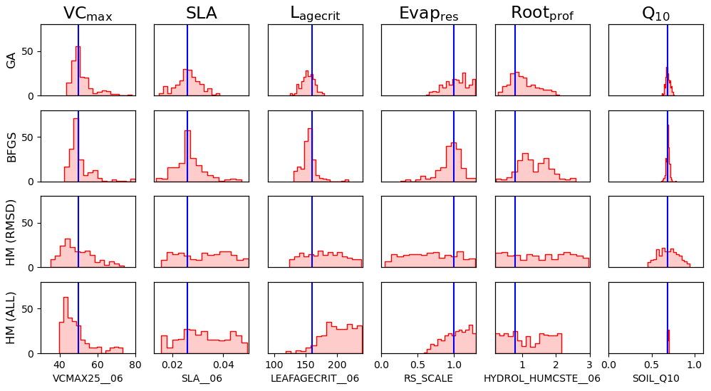
Figure C2 1-dimensional representation of posterior parameter distributions. For the data assimilation experiments (GA and BFGS), the values represent the results from the stochastic experiments (i.e. from 200 optimisations). For the history-matching experiments (HM; RMSD for when only the RMSD metric is used; ALL for when all the metrics are applied), 200 parameter sets were sampled from the 𝒳_NROY. The true values are shown in blue.