the Creative Commons Attribution 4.0 License.
the Creative Commons Attribution 4.0 License.
 | 31 Jul 2024
A new 3D full-Stokes calving algorithm within Elmer/Ice (v9.0)
Douglas I. Benn
Anna J. Crawford
Joe Todd
Thomas Zwinger
A new calving algorithm is developed in the glacier model Elmer/Ice that allows unrestricted calving and terminus advance in 3D. The algorithm uses the meshing software Mmg to implement anisotropic remeshing and allow mesh adaptation at each time step. The development of the algorithm, along with the implementation of the crevasse depth law, produces a new full-Stokes calving model capable of simulating calving and terminus advance across an array of complex geometries. Using a synthetic tidewater glacier geometry, the model is tested to highlight the numerical model parameters that can alter calving when using the crevasse depth law. For a system with no clear attractor at a pinning point, the model time step and mesh resolution are shown to alter the simulated calving. In particular, the vertical mesh resolution has a large impact, increasing calving, as the frontal bending stresses are better resolved. However, when the system has a strong attractor, provided by basal pinning points, numerical model parameters have a limited effect on the terminus evolution. Conversely, transient systems with no clear attractors are highly influenced by the choice of numerical model parameters. The new algorithm is capable of implementing unlimited terminus advance and retreat, as well as unrestricted calving geometries, applying any vertically varying melt distribution to the front for use in conjunction with any calving law or potentially advecting variables downstream. In overcoming previous technical hurdles, the algorithm opens up the opportunity to improve both our understanding of the physical processes and our ability to predict calving.
- Article
(5678 KB) - Full-text XML
-
Supplement
(36786 KB) - BibTeX
- EndNote


One of the largest sources of uncertainty in predictions of future sea level rise is the magnitude of losses from the Greenland and Antarctic ice sheets via ice discharge and iceberg calving (IPCC, 2023). In recent years, significant advances have been made in understanding calving processes and their relationship with ice dynamics (Benn and Åström, 2018), but this has yet to translate into the adoption of a reliable, universal “calving law” in continuum ice sheet models. This largely reflects the contrast between the complexity of calving processes, which are influenced by stresses in three dimensions, and the simplified, vertically integrated stress fields required in model simulations of long-term and large-scale ice sheet evolution. There is a need, therefore, to develop robust, physically based calving models in three dimensions which can then be used to develop simpler calving parameterisations required for ice sheet models that apply approximations to the Stokes equations.
Currently, there are two main types of 3D calving modelling methods with the capability to simulate the evolution of glacier calving fronts through time. The first is discrete-element modelling (DEM), which is commonly referred to as particle modelling. An example model is the Helsinki Discrete Element Model (HiDEM) which predicts calving from first principles by treating the ice as elastically bonded individual particles, where the bonds fracture if a failure threshold is exceeded (Aström et al., 2014). HiDEM can accurately simulate a wide range of individual calving styles but is unsuitable for modelling longer-term glacier evolution because it does not include viscous deformation (Åström et al., 2013; van Dongen et al., 2020; Benn et al., 2023). Conversely, glaciers can be modelled as continua in 3D using a model such as Elmer/Ice. Elmer/Ice is a finite-element method (FEM) model that treats the ice sheet as a continuum and solves the flow and stress fields using the full-Stokes equations. Using the position-based crevasse depth calving law, Elmer/Ice has been shown to accurately predict calving front evolution at Store Glacier (Sermeq Kujalleq) in response to changing fjord conditions (Todd et al., 2018; Benn et al., 2023). Although the computational requirements of Elmer/Ice remain high, they are significantly lower than the requirements of HiDEM, and multiple years of calving front evolution can be simulated with reasonable computational resources (Todd et al., 2018, 2019).
However, several issues remained with using the Elmer/Ice calving model, as implemented by Todd et al. (2019), to run multi-year simulations. First, the lateral corners of the ice front (i.e. where the calving front meets the fjord wall) were fixed in place. This is a reasonable assumption for stable glaciers such as Store Glacier (Sermeq Kujalleq), where only the seasonal movement of the calving front needs to be captured (Todd et al., 2018). However, in the most extreme warming experiments conducted for Store Glacier, the simulated retreat caused model breakdown due to the restriction that the lateral boundaries of the front were fixed in space (Todd et al., 2019). The assumption of fixed lateral boundaries does not hold for fast-retreating glaciers such as Jakobshavn Isbræ (also Sermeq Kujalleq in Greenlandic), where the terminus position may change year on year by several kilometres (Joughin et al., 2020). Furthermore, the Todd et al. (2019) model relied on a 2D vertically extruded mesh, which is problematic where the ice front is non-vertical, such as where submarine melt produces undercutting (Todd et al., 2019). As a result, ice front retreat leads to the degeneracy of the mesh elements, which causes irrecoverable breaking of the calving model. The importance of submarine melt is often associated with its known ability to increase calving (O'Leary and Christoffersen, 2013). However, investigating the importance of the submarine plume melt undercutting on calving is only possible in a 3D calving model because of the importance of terminus geometry and as such has remained understudied. Finally, Todd et al. (2018) assumed the projectability of the calving front and calved icebergs, namely that the post-calving ice front does not contain any complex re-entrants and can therefore be projected onto a transverse plane. This is clearly not always the case at real glaciers, particularly those with complex front geometries such as Bowdoin Glacier (Kangerluarsuup Sermia), Greenland.
This paper presents a new calving algorithm that rectifies these limitations. It utilises 3D remeshing which is implemented using the open-source remeshing algorithm Mmg (Dapogny et al., 2014). The level set method is used to define areas of calved ice (Osher and Fedkiw, 2001; Sethian, 1999), and the new calving front is physically implemented using Mmg. In this paper, the key steps and processes involved in the new algorithm are outlined, leading into an explanation of how the algorithm resides within the framework of a typical glacier simulation. The capabilities of the new algorithm are described and illustrated using a set of synthetic glacier geometries with a particular focus on the use of the crevasse depth calving law. The new algorithm allowed a more detailed study using the crevasse depth law to assess the influence of the model setup on predicted calving, along with demonstrating the theoretical implications of the calving law. Furthermore, the often neglected numerical model parameters with the potential to alter modelled calving are investigated, providing a sound basis for rational parameter choices in future studies using real-world domains. Mesh resolution, model time step, and adaptive time stepping are investigated. The impact of each numerical model parameter is investigated and discussed within the context of the crevasse depth calving law. Finally, the capabilities of the new model are concluded.
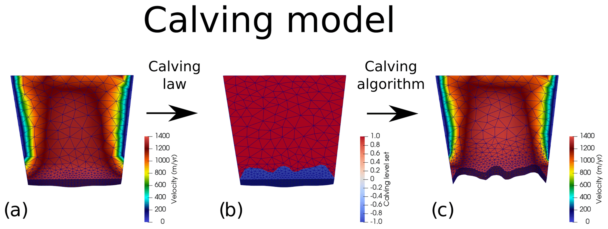
Figure 1Illustrating the difference between the calving model, algorithm, and law. (a) The initial flow solution. The calving law predicts calving based on the solved variables on the initial geometry. (b) The predicted calving based on the calving law. This prediction is in the form of a level set variable which is then fed to the calving algorithm. Nodes with a negative value (in blue) show areas to be calved, and those with positive values (in red) show the remaining glacier domain. (c) The new geometry with all the variables interpolated across (from (a)) showing the interpolated velocity field. The calving model represents the combination of both the calving law and algorithm, allowing one to go from panels (a) to (c).
When modelling calving, it is important to distinguish between the calving law, calving algorithm, and calving model (Fig. 1). The “calving law” is the function by which calving is predicted, in this case the crevasse depth (CD) law (Nick et al., 2010; Benn et al., 2007). The “calving algorithm” takes the prediction from the calving law and implements this within the model, ultimately leading to the removal of calved ice and the resulting alteration of the domain. Consequently, a calving algorithm is not tied to a particular calving law. Instead, it is the technical implementation, within a given ice flow model, of a theoretical calving event provided by the independent calving law. Putting the calving law and calving algorithm together gives us the “calving model”. This is an important distinction to make within glacier modelling, as both calving laws and calving algorithms are limited in their functionality at this time. Calving laws in 3D can be thought of as resulting from a combination of our current understanding of the physical processes behind calving and our ability to condense them into a mathematical function compatible with the ice flow model. Calving algorithms can be viewed as the capability of our models to implement the calving law's prediction on a given domain by removing the predicted calved ice. This is surprisingly non-trivial, especially for more advanced calving laws that can produce convoluted calving geometries. This paper focuses on the development of a new calving algorithm that substantially increases our ability to realise calving in a 3D glacier model. This is primarily motivated by our previous limited ability to simulate the substantial retreat and advance of fast-flowing glaciers in 3D. The objective is that once the previous technical hurdles have been overcome, our understanding and capability to test calving laws and physical processes can correspondingly be improved. In this paper, we implement the CD calving law in connection to our newly developed algorithm, thus defining our calving model. The CD law was chosen because it is the only currently available calving law that is explicitly based on physical processes with a proven capability for predicting calving on Greenland tidewater glaciers (Todd et al., 2019; Amaral et al., 2020; Benn et al., 2023). The CD law is based on the idea that calving occurs when crevasses penetrate the full thickness of the glacier or some prescribed part thereof (Benn et al., 2007; Nick et al., 2010). For simplicity and ease of implementation, crevasse depth is predicted using the zero-stress approach introduced by Nye (1957) and modified by Todd et al. (2018), which assumes that fracturing is possible wherever the largest principal stress σ1 (the largest eigenvalue of the Cauchy stress) is extensional (positive). This approach assumes negligible stress concentrations at crack tips, which is reasonable for fields of closely spaced crevasses. Calving is thus a function of the large-scale stress field of the glacier and particularly regions of high extensional stress. It is important to emphasise that the CD law does not predict individual crevasses or impose discontinuities on the model glacier. Rather, the zero-stress function defines bounding surfaces of crevasse fields (i.e. the base in the case of surface crevasses fields and the top in the case of basal crevasses fields), which are then used to predict the position of the glacier front at a particular time step.
Implementing any calving law in a continuum model requires the new position of the ice front to be prescribed at each time step. In vertically integrated models, this is relatively straightforward because the ice front is by definition vertical before and after calving, and the model physics can be solved on a 2D mesh. The problem becomes substantially more difficult in three dimensions when the front can have complex vertical profiles due to melt-undercutting or deformation.
Representing the change in the glacier domain via calving can either be done by an explicit change in a domain (i.e. modification of a mesh) or by using a “calving variable” that represents the new terminus position. Computationally, it is much cheaper to use a variable since only this variable needs to be manipulated prior to calculation of the new flow solution. This approach is becoming increasingly popular, especially among lower-level models in which the computational efficiency is the priority (e.g. Bondzio et al., 2016). Usually, this is done using a level set method (Osher and Fedkiw, 2001; Sethian, 1999; Bondzio et al., 2016) where a surface is defined from a signed distance and moves based on an advection equation. The main drawback of this method is the need to solve intra-element dynamics if a level set surface is to be followed exactly, since the hyperplane will cut through any form of element. No current model has the capability to solve this problem, which would require boundary conditions to be applied across the hyperplane (e.g. Bondzio et al., 2016). Instead, intersected elements are marked; those beyond are marked as ice-free and those in the glacier domain marked as ice. Boundary conditions are instead applied across the ice-free boundary of the intersected elements, so the actual modelled calving front generally deviates from the level set surface (Bondzio et al., 2016).
Alternatively, explicit domain change is more computationally expensive and significantly more complicated to implement. Simplistically, this can be achieved by deforming the mesh (i.e. moving nodes but keeping the mesh topology intact), but this can only be done for non-complex geometries and becomes less feasible with more dimensions and more significant deformations. Complex problems require complete remeshing through which element edges are realigned along the new calving front. Todd and Christoffersen (2014) produced a flowline 2D model with complete remeshing that allowed a non-vertical terminus but concluded that all three dimensions needed to be considered for accurate calving representation. A similar approach was taken by Berg and Bassis (2022), where the vertical dimension was seen as imperative to the study of calving dynamics and ice history. The most advanced example is the 3D extruded remeshing implemented by Todd et al. (2018). Despite the increased complexity, several advantages emerge from this approach. For example, complete remeshing allows a finer resolution to be maintained near the calving front if the terminus moves greatly over the course of the simulation. Second, the position of the calving front resembles that defined by the calving law much more closely, allowing the implementation of more complicated position-based calving laws.
The CD law is designed to predict the position of the ice front at each time step based on the ice geometry and stress field. However, the predicted front may also be influenced by numerical model parameters such as time step and mesh resolution. Like any computational method, FEM requires a model time step that represents the time gap between the calculation of the model physics. Usually, the time step must be small enough to meet the Courant–Friedrichs–Lewy (CFL) condition (Courant et al., 1928) as it applies to the evolution of the free surfaces. Furthermore, changes in the time step can alter the numerical solution, with coarser time steps often reducing accuracy. Similarly, changes in the mesh resolution can alter the numerical solution of the problem with smaller elements allowing greater gradients across the domain. Limited research has reported on how numerical model parameters influence model results; the experiments conducted in this study provided an opportunity to analyse the effect of these parameters on both the new calving algorithm and the CD law.
In this paper, we illustrate the features and capability of the new algorithm using a simple synthetic geometry broadly representative of a Greenlandic glacier but with reduced computational costs. The synthetic glacier is dominated by strong shear margins with super-buoyant sections of the terminus. All of the experiments in this paper were completed on a local desktop with Intel Xeon Processor E3-1245 v5 using eight threads. The control simulation took 45 min to simulate 106 time steps (100 d time steps plus 6 adaptively added), and the final domain had a maximum of 35 980 degrees of freedom. Simulation time scaled linearly with an increase in time steps and cubically with an increase in 3D mesh resolution. The full geometry and input files can be found in the official Elmer/Ice repository (https://github.com/ElmerCSC/elmerfem, last access: 29 July 2024) or in Wheel (2023a) in the test case elmerice/Tests/Calving3D_lset. Full details of the associated geometry and boundary conditions are detailed in Appendix A. Rather than giving the unrestricted details and coding design associated with the algorithm, the key methodological choices and model capabilities are presented here, highlighting their benefits and drawbacks. A comprehensive breakdown of the algorithm and minor coding choices is provided in the Supplement or in Wheel (2023b). Detailed user documentation is provided in the Elmer/Ice repository or in Wheel (2023a).
4.1 Explicit domain modification
The domain of a glacier actively evolves through three mechanisms: (1) movement of the glacier terminus via ice flow countered by frontal melting; (2) retreat of the terminus via iceberg calving; and (3) elevation of the surface and base of the glacier evolving through ice thickness advection, melting, or accumulation. The implementation of the movement of the terminus, base, and surface boundaries is achieved through deforming the mesh while calving is implemented through remeshing.
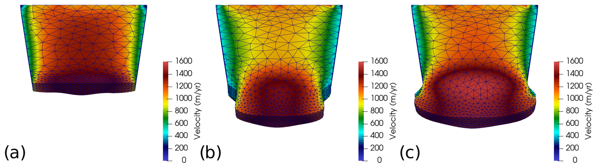
Figure 2Two examples showing the capabilities of the front advance routines over 1-year simulations. Calving is suppressed for both simulations so the resultant geometry is purely from glacier advance. (a) The initial geometry prior to simulation. Final geometry and velocity field for (b) a narrowing fjord and (c) a widening fjord. The full simulations can be seen in Videos 1 and 2 in the Supplement.
4.2 Mesh deformation: terminus advance and free surfaces
The Lagrangian advection of the terminus for a given time step is computed using the velocity solution. For constricted domains such as glaciers flowing down a fjord, the advance of the lateral margins take account of local geometry. Across the majority of the terminus, the displacement vector (d) is the velocity multiplied by the time step. However, where the calving front and the lateral boundaries meet, the displacement vector cannot be based purely on the velocity, since the terminus advance must be constrained by the fjord walls and by imposed kinematic constraints. This could be solved as a contact problem analogous to the grounding line (Durand et al., 2009), but this would increase the computational requirements as the non-linearity of the problem increases. Instead, fjord walls are user-defined before the simulation. For each time step after the calculation of the flow solution, the velocity is reprojected along the predefined fjord walls (see Fig. 5 for the solver order). As such, the displacement in the x and y plane at the lateral margins (dl) is defined by
where u is the velocity, and f is the tangential direction of the fjord wall. Currently, the fjord is only represented in the x and y plane rather than a 2D surface. Although this is very computationally efficient, it provides some sources of error. First, the normal vector is poorly defined on the lateral corners where the terminus meets the lateral boundary. Additionally, even though the velocity follows the local lateral boundary, this does not guarantee that it will follow the boundary further downstream as the glacier advances. Therefore, it may lead to artificial mass change as the imposed kinematics of the lateral boundary corners are not guaranteed to obey the incompressibility condition. This artificial mass change is negligible, especially when compared to mass changes associated with remeshing. This provides a much better solution than having the lateral corners fixed in place and time (Todd et al., 2018). The mesh is deformed horizontally using the predicted front advance as a boundary condition. Similarly, the kinematic free surface is calculated for the surface and base before the mesh is deformed vertically using these solutions. This accounts for the glacier surface mass balance, while the grounding line evolution is solved as a contact problem (Durand et al., 2009). In order to simulate terminus advance through complex fjord geometries, the model has the capability to transfer boundary elements from the terminus to the lateral boundary. For example, when the glacier advances down a narrowing fjord, the Lagrangian movement of the terminus means it will make contact with the prescribed fjord wall. Here, if all nodes in a boundary element reach the fjord wall, the model will change the conditions applied to the element from those of the terminus to those of the lateral boundary. The model can replicate a realistic advance at widening and narrowing fjords while maintaining the appropriate boundary assignment (Fig. 2).
Similar to the terminus advance, the retreat due to submarine melting can be applied to the calving face. It is applied as a scalar variable, where the direction of melt is always assumed to be normal to the terminus nodes based on adjacent elements. Following the Lagrangian implementation of the glacier advance, melt is prescribed such that
where is the melt normal to the front. As the terminus normal will not follow the lateral boundary, some artificial mass change is introduced at the lateral boundary corners. Again, this is negligible when compared to mass changes from remeshing. Melting with any vertical or horizontal profile can be implemented, the calculation of which is independent of the calving algorithm. Given the simplicity of this method, there are very few issues that can arise when applying melt. Degenerate elements will only be produced if the melt per time step is larger than the element length in the normal direction. In other words, Eq. (2) must comply with the CFL condition for the front.
4.3 Calving through remeshing
The calving algorithm is defined as the implementation of calving or the removal of ice from the glacier front. It takes a level set or signed distance variable for which the zero contour is the new calving front to produce a new mesh onto which all the model variables are interpolated. Importantly, the new calving algorithm is not limited by iceberg or frontal geometries and consequently is not tied to a particular calving law. Given its physical basis and use as a position-based law, the CD law is a particularly complex calving law to apply in a 3D model. It therefore provides a high benchmark, and simpler rate-based laws could easily be applied. The CD law is implemented following Todd et al. (2018), but improvements allowing non-projectable calving have been made through use of a level set function (Osher and Fedkiw, 2001; Sethian, 1999). For further details, see the user documentation detailed in the “Code and data availability” section at the end of the paper. To overcome these issues, the remeshing software Mmg (version 5.5.4 or later) is used in the new calving algorithm to produce a fully 3D domain without the need for vertical extrusion (Dapogny et al., 2014). To use the calving algorithm, Mmg must be compiled and linked with Elmer.
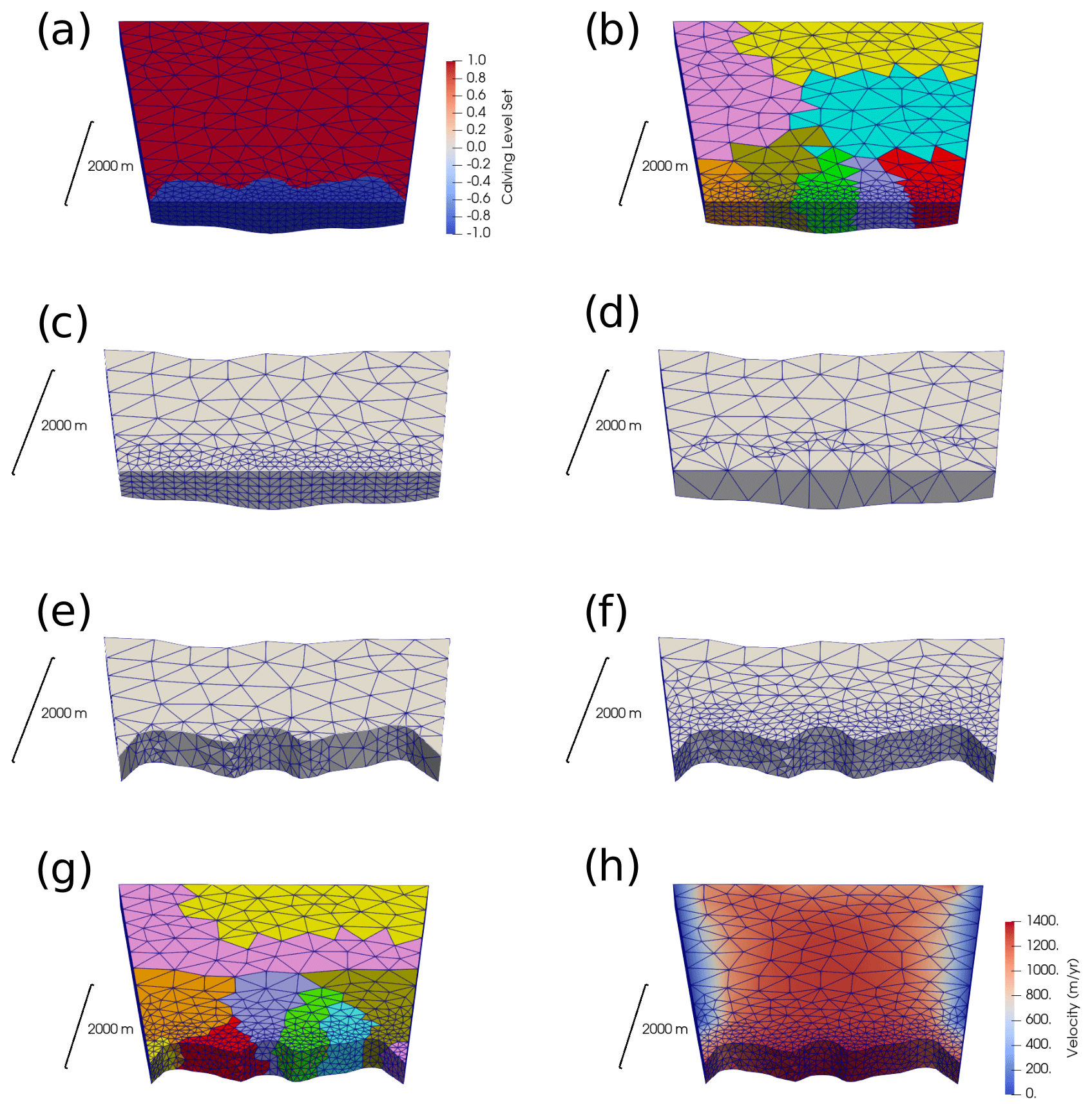
Figure 3A visualisation of the steps involved during remeshing in the calving algorithm for a simulation run on eight cores. (a) The 3D glacier mesh showing the calving level set variable defining the predicted calving. The reduced range of the calving level set variable is just to clearly show the predicted calving. (b) The same distributed mesh showing the eight partitions. (c) The gathered mesh on one core. The upstream size is defined by the user-defined remeshing distance from the new calving front. (d) The first remeshing step in which the element edges are aligned along the new calving front, as predicted by the calving level set variable shown in panel (a). (e) After the first remeshing step, the nodes with negative calving level set values are cut (e.g. glacier ice that would calve as icebergs is removed). (f) The second remeshing step through which the mesh quality is improved. (g) After remeshing, the mesh is rebalanced so that each partition has a computationally equivalent partition. (h) The variables are interpolated to the new mesh in parallel, and the old mesh is deallocated from memory.
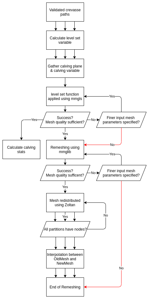
Figure 4Diagram outlining the steps involved in the calving algorithm. A visual representation of an example simulation can be seen in Fig. 3. Red arrows indicate paths where calving is suppressed. Single arrows indicate stages which occur in series, and three arrows indicate stages that can occur in parallel.
Currently, remeshing is completed in two separate steps. The first step realigns element edges along the zero-level-set contour. This will be referred to as implementing the level set variable. The second stage is complete anisotropic remeshing to improve the mesh quality where a user-defined aspect ratio produces elongated elements in the horizontal plane. The full remeshing algorithm is visualised in Fig. 3 and outlined in Fig. 4. To reduce the computational requirements, only the area within a user-defined distance from the terminus is remeshed. In a parallel run, the Elmer mesh partitions must first be gathered onto one process (Fig. 3b and c) as Mmg must be run in a series. Essentially, for both remeshing stages, the nodes and elements on the upstream partition boundary of the gathered mesh are fixed and cannot be altered. This means that when converted back into the Elmer mesh format, the new mesh still has the same partition boundaries with the upstream parts of the mesh which have not been altered. In a parallel run, the gathered mesh must be redistributed using the library Zoltan (Devine et al., 2009) or using ParMETIS, which provides much better balancing for larger jobs. A rebalancing algorithm aims to rebalance the mesh evenly in terms of computational requirements among all active processes whilst trying to reduce parallel communication (Fig. 3f). After the rebalancing, variables from the old mesh are interpolated across the new mesh in parallel (Figs. 3 and 4). Surface and bottom-boundary variables are projected from the old mesh. Both surfaces must maintain projectability to allow the free surface to be solved. However, with the possibility of complete remeshing, there are occasionally sections of the surface and bottom boundaries that are not covered by the old mesh. Nodes here are individually extrapolated.
Iceberg calving and fracture happen far below the typical glacier model time steps, and consequently, secondary calving is often omitted from calving simulations. Secondary calving occurs when iceberg removal leads to a geometry change that is inherently mechanically unstable and so produces further calving. To overcome this issue, the new calving algorithm can insert additional small time steps to facility secondary calving where the new glacier geometry is assessed to see if it produces further calving. The size of the additional time step and the calving volume threshold to invoke extra time steps are user-defined. These additional calving time steps allow the calving cycle to be complete prior to the model moving on to the next true time step.
4.4 Robustness of algorithm
Given the complexity of potential geometries arising from calving at a tidewater glacier, it can be expected that instances of remeshing failure will occur during simulations. Remeshing failure can be defined as the inability to produce a mesh of sufficient quality to allow the continuation of the simulation. It is not possible to prevent this for every scenario that may arise, so additional focus must be placed on the robustness of the calving algorithm to cope with remeshing failure. A major advantage of performing the level set variable implementation and anisotropic remeshing in two steps is the ability to isolate a source of potential failure. If there is an issue with either step, the process is retried with finer-mesh input parameters. This often results in success (Fig. 4). This feature allows the user to specify multiple input parameters, such as the minimum element edge length, which can be iterated through until remeshing success occurs.
Remeshing failure can occur for several reasons. The first reason is that Mmg is unable to return a mesh. Second, remeshing failure can occur if the element quality does not meet the user-defined minimum quality. However, there can be times when level set implementation fails for all user-specified input parameters (Fig. 4). Calving cannot occur in this case since the new terminus boundary is not defined. Remeshing still occurs to try to improve the mesh quality. Similarly, if remeshing fails on all input parameters, then calving does not occur – even if the level set variable implementation has been successful (Fig. 4). Both situations can lead to the glacier falsely advancing. This is not a major issue as calving will likely occur during the subsequent time steps.
A final potential issue with the remeshing can result if a mesh passes through the various quality checks but has some physical imperfection or poor element quality that leads to problems in the Stokes solver. Element quality checks attempt to prevent such instances but are not fool proof. Such imperfections often cause unrealistic velocity solutions, leading to an exaggerated stress distribution that in turn can cause unrealistic calving events. An additional step in the calving algorithm has been added to check the new flow solution. The convergence of the velocity solution, maximal velocity, and divergence from the previous time step are checked against user-defined limits, which ensures that a mesh imperfection does not slip through. Finally, model check pointing, by regularly saving the model state, allows easy recovery in case of simulation breakdown.
If the flow solution is determined to be inadequate (non-converged), then the mesh deforming and calving solvers are suppressed, except for the anisotropic remeshing routines. The mesh input variables are refined, and the flow solution residuals are removed, so that the velocity is calculated from scratch. These refinements result in a finer mesh and an extension of the remeshing distance. The latter is extended in case the fixed elements are causing the flow convergence issue. Additionally, the model time is set back to the time at the start prior to the current, problematic, time step plus 1 s (Fig. 5). The additional second allows the time-dependent solvers to be rerun while changing the model time by an insignificant amount in a glacier context. An extra time step is added to the required time steps for the simulation. Following the subsequent remeshing step, the mesh quality will usually have improved enough to provide a flow solution. At this point, the solver will unpause the mesh deforming and calving solvers and reset the mesh input variables to their original values (Fig. 5).
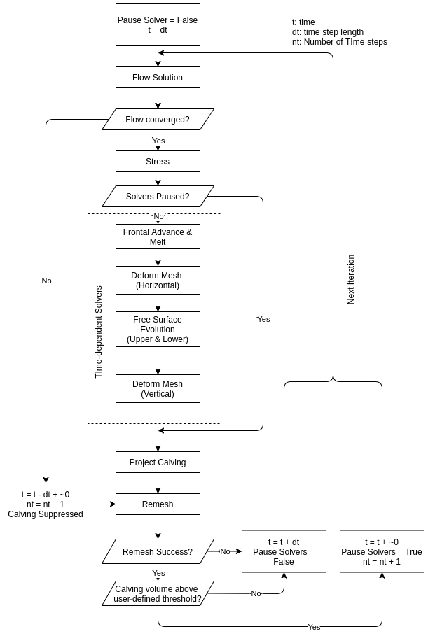
Figure 5Diagram showing the stages involved in a typical simulation using the calving algorithm and front advance routines in tandem.
A typical simulation is now outlined, putting together the new advance, calving, and remeshing mechanisms (Fig. 5). After the model initialisation and set up, the solvers follow the new algorithm. First, the velocity field is solved. It is then checked to assess it for any abnormalities. If abnormalities exist, then the recovery mechanisms outlined above are followed.
Assuming that the flow solution converges, it is used to solve the stress fields from which calving is predicted by the CD law. After the calving prediction, the top and bottom free surfaces are solved using the built-in Elmer free-surface solver. As outlined previously, the terminus advance is calculated from the flow solution. Using these variables, the glacier mesh is deformed both vertically and horizontally. Ideally, the flow solution would be recalculated after the front adjustment since the calculated velocities are based on a different geometry. This means that, currently, the calving prediction is based on the stress field that was calculated for a slightly different geometry. This purely explicit in time approach is used currently to save computational requirements. Unless time steps are extremely large for the size of the domain, this should not impact the results.
After the mesh deformation stage, the calving algorithm is called. If remeshing is unsuccessful at any stage, calving is suppressed, and the model moves onto the next time step. Following recovery through successful remeshing, any solvers that were previously paused are turned back on, and the time step is checked to make sure it is the original input. If remeshing is initially successful but only insignificant calving occurs, the time step is not altered. However, if an iceberg calves above the user-defined threshold, mesh-deforming solvers are paused, the time step is reduced, and an additional time step is added to the model to allow the simulation to run for the required time (Fig. 5). To summarise, the model time step can be altered for two reasons: (1) as a safety check following a non-converged or unrealistic flow solution allowing the model time step to be rerun or (2) the reduction in the time step following a large calving event to check if subsequent calving can occur. Henceforth, the latter is referred to as adaptive time-stepping. The time step cannot be adaptively increased; instead, it is returned to the original time step when the above conditions are not met.
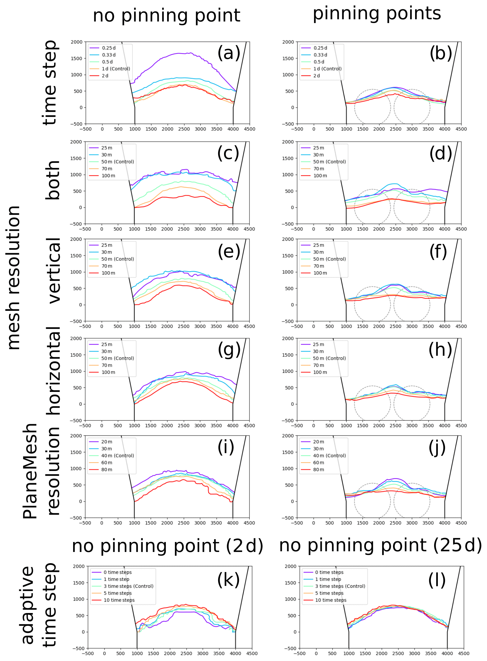
Figure 6Terminus positions at the end of the experiments altering numerical model parameters. Panels (a), (c), (e), (g), (i), (k), and (l) were run on the domain with no pinning points and panels (b), (d), (f), (h), and (j) with basal pinning points. The numerical model parameter altered for each simulation shown were (a, b) time step magnitude, (c, d) horizontal and vertical mesh resolution, (e, f) horizontal resolution, (g, h) vertical resolution, (i, j) PlaneMesh resolution, and (k, j) adaptive time-stepping. The mean retreat rates are presented in Table 1.
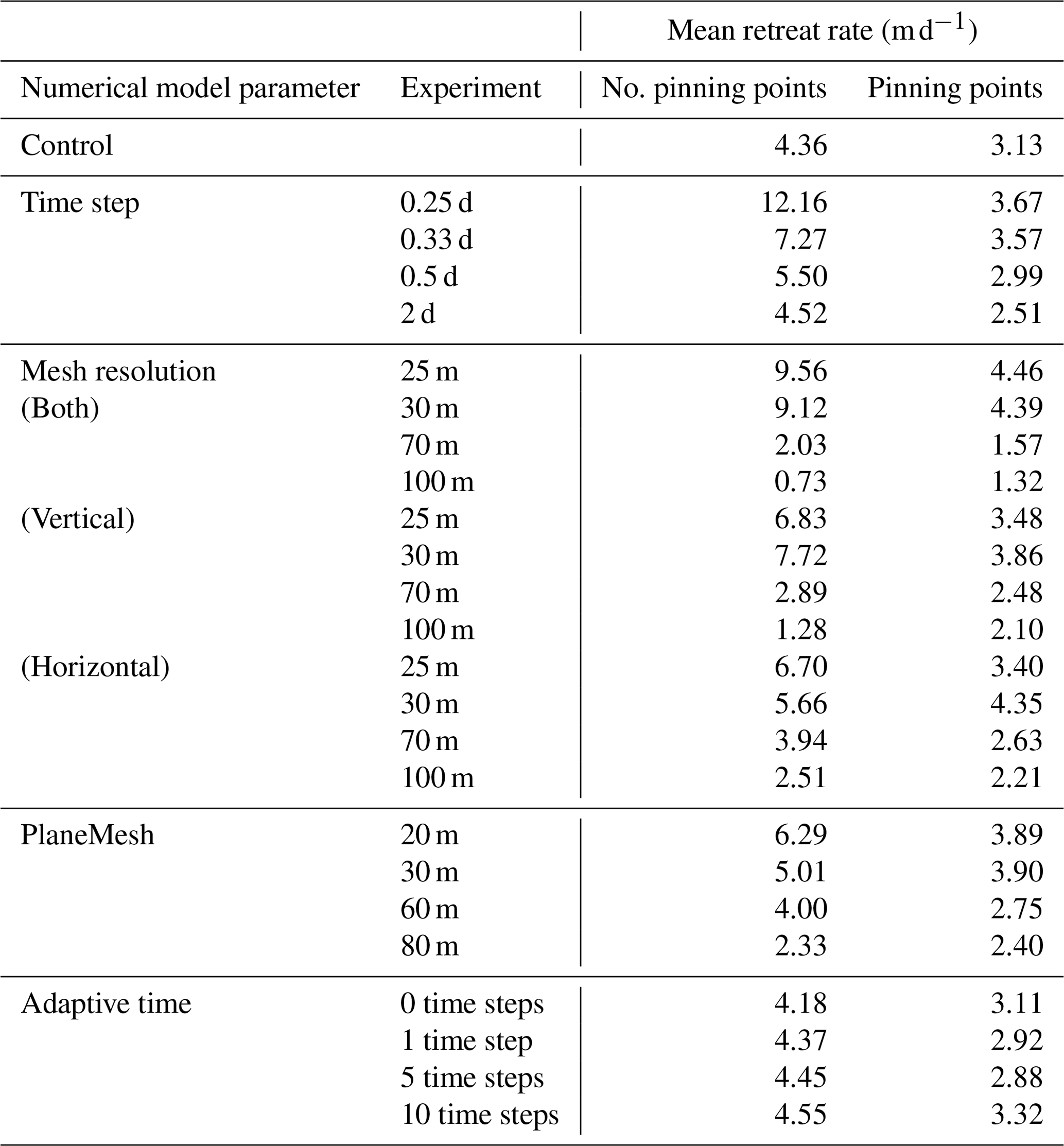
Predictions of the calving front position depend not only upon the physical setup and tunable parameters such as crevasse penetration threshold but also on numerical model parameters such as time step and mesh density. Numerical model parameters can potentially affect the results through the calving algorithm or the characteristics of the chosen calving law. Experiments were run to assess the impact on the calving algorithm by varying the time step magnitude and mesh density in runs using a simple rate-based law. These showed insignificant variations in the predicted retreat rate (± 0.01 m d−1; Appendix B). Consequently, the focus of the experimentation is on the variability provided by the CD law, which provides a better representation of calving processes. Conceptually, the CD law predicts the stable ice front position for any given position and tends to converge on attractors at pinning points (Benn et al., 2023). In order to best show how non-physical factors within the numerical system can alter the predicted calving, two synthetic domains were created. The first has a sloping bed with no bed irregularities producing a system lacking a strong attractor. The second has two basal rises (i.e. potential pinning points) near the initial terminus position which act as an attractor within the system. The model setup is described in Appendix A. Note that the location of the basal rises produces an asymmetric geometry. The control value for each parameter is described at the start of the relevant section. Mean retreat rates were calculated as the mean displacement of the terminus per time step along the y axis.
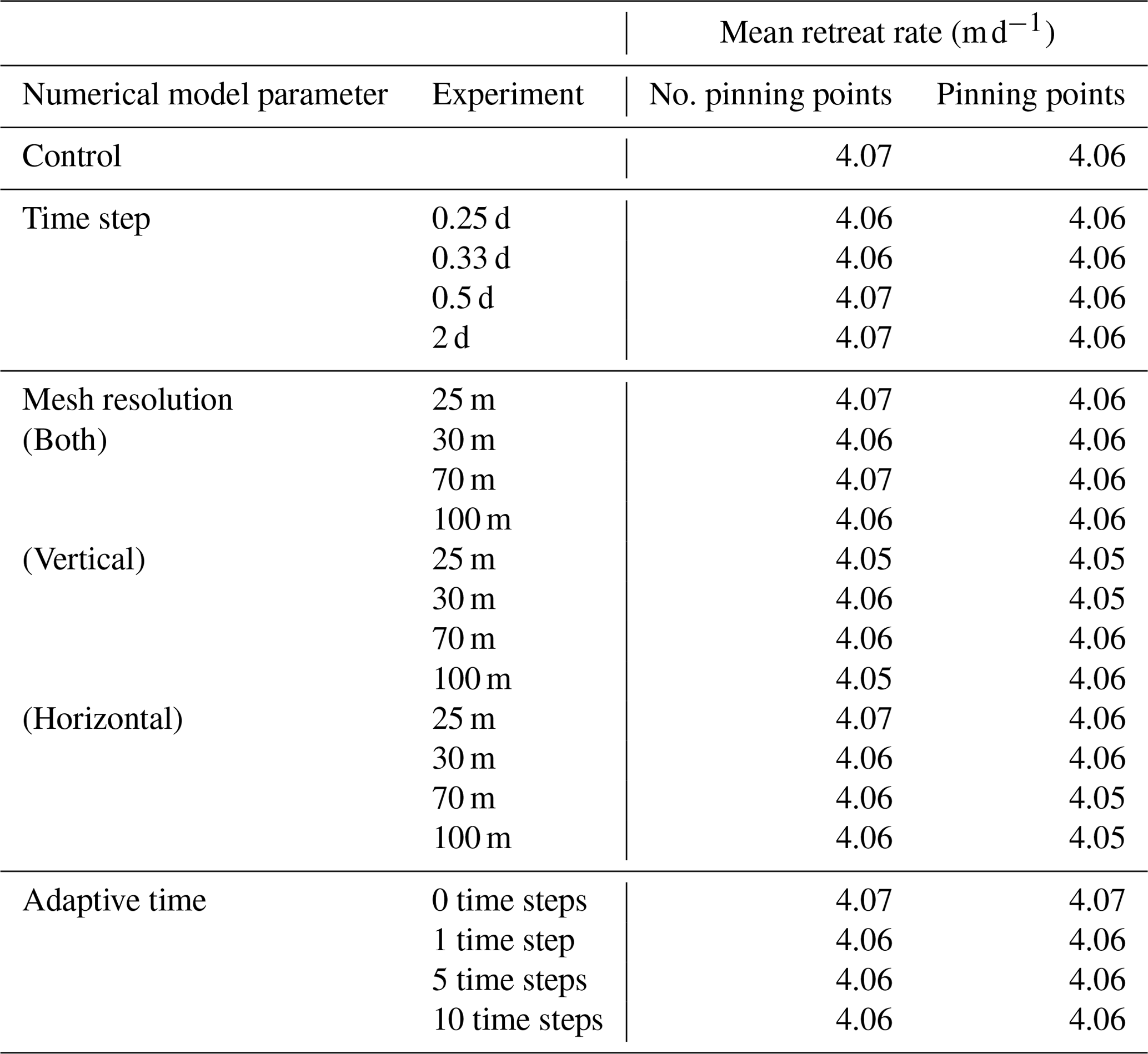
Table 1Summary of the mean retreat rates for 100 d experiments testing the numerical model parameters that can alter calving.
6.1 Time step magnitude
The use of a position-based calving law, which calculates the ice front location from an instantaneous state of the evolving glacier geometry and stress field, means its solution could be affected by the assigned time step. Although rate-based laws will also be time-step-dependent, often through the evolution of the glacier-free surfaces, they do not inherently aim to predict the attractor point in the retreat. As noted above, the duplicate experiments using a rate-based law were insensitive to time step changes. In contrast, the CD law aims to predict the position at which the glacier stabilises and so will potentially be sensitive to the time step when the glacier is in a transient state.
Four additional simulations with time steps of 2, 0.55, 0.33, and 0.25 d were run to complement the control simulation with the time step of 1 d (Fig. 6a and b). All the simulations ran for a total of 100 d. The initial calving event on the first time step remains similar irrespective of the assigned time step. For all runs, the glacier underwent retreat, but the rate of retreat increased as the time step decreased when no pinning points were present. There is no clear convergence with each reduction in the time step leading. In contrast, when pinning points are present, the magnitude of retreat no longer increased with a decrease in the time step beyond 0.33 d. Further reduction in the time step to 0.25 d does not yield further retreat. Notably, when pinning points are present, all the experiments showed very similar terminus positions and shapes (Fig. 6b).
The increased calving modelled when smaller time steps were applied can be explained by the increased number of times that calving was predicted. As the time step reduces, the frequency of computing the stress field on a unique geometry increases. This increased frequency of calving prediction increases the modelled calving because it heightens the probability of successful calving. For a glacier system with no strong attractor, calving is highly dependent on the time step. When an attractor is added, in the form of pinning points, the predicted calving is much less sensitive to the model time step. Diminished returns are seen, and the retreat did not increase when reducing the time step beyond 0.33 d. Care should therefore be taken when using the CD law to model transient behaviour to choose the appropriate model time step. The time step is of less importance when an attractor is present, as the general form of the retreat is consistent regardless of the time step.
6.2 Adaptive time step
The calving algorithm can add additional, shorter time steps if large calving events occur to determine whether the calving-induced change in geometry will lead to further, immediate calving (Fig. 5). The control simulation could add up to three additional small time steps of 1 × 10⁻¹⁰ years if the calving threshold, set as 1 × 10⁷ m3, was reached at the prior time step. Four further simulations were done for each domain; the first was done with the adaptive time stepping deactivated, and the other three experiments were set to enable up to 1, 5, or 10 additional time steps (Fig. 6k and l). The calving threshold at which the adaptive time stepping was invoked, and the additional small time step sizes were not changed from the control.
Without the adaptive time step, the terminus initially retreated at a slower rate but ultimately reached the same stable point as the control, regardless of the domain (Fig. 6k and l). The positions for the more sensitive domain without pinning points are shown (Fig. 6k and l), but when pinning points are present, the ultimate terminus also matches the control. Conversely, with more adaptive time steps, the terminus retreated at a quicker rate from the unstable starting geometry. Over time, the terminus positions slowly converged towards the same position where, at 25 d, they are almost identical (Fig. 6l). From 25 d until the end of the simulation at 100 d, the terminus positions do not diverge.
Adaptive time stepping intuitively makes sense, based on our knowledge of secondary calving, and so is important if a time series of terminus positions is wanted. If, instead, only the ultimate terminus position for a longer-term simulation is required, then it is unlikely that adaptive time stepping will change the result. Therefore, when using the adaptive time stepping functionality, it is important to consider the topic of investigation and timescales of interest for the simulation.
6.3 Glacier mesh density
As previously stated, the choice of mesh density is usually determined by the CFL criterion corresponding to the assigned time step in glacier simulations. Increased horizontal and vertical resolution can refine the flow and stress solution, especially at areas of high shear or tensile stress. In the simulations shown in this paper, the smallest elements were closest to the glacier terminus where bending and extensional stresses are prominent and essential for determining calving locations. Increased mesh density comes at a computational cost and increases cubically as the resolution increases. This is because doubling the resolution quadruples the number of elements in the mesh. Usually mesh density is dictated by computational resources, but the small synthetic geometry used in this testing allows us to further investigate changes in the mesh resolution.
Experiments with varying mesh densities were conducted for both domains (Fig. 6e–h). The control had a vertical and horizontal mesh resolution of 50 m at the terminus, and additional simulations were run with mesh resolutions of 25, 30, 70, and 100 m. Vertical and horizontal mesh resolution were investigated independently and collectively produced 12 experiments for each domain (Fig. 6e–h).
Increased glacier mesh density led to increased retreat across the terminus in the absence of a pinning point (Fig. 6e). When pinning points were present, although an increased mesh density led to increased retreat, the retreat is limited to where the glacier is pinned. A reduction in the glacier mesh density limits the retreat on both domains. Independently changing the horizontal resolution had a limited impact on calving in either domain. The vertical mesh resolution has a far larger impact accounting for most the retreat seen when the mesh resolution is increased across both planes (Fig. 6g and h).
The vertical resolution had a much larger impact on calving because this parameter alters the penetration of basal crevasses as – depending on the resolution – more or fewer elements are present near the waterline. Greater resolution allows the ice cliff imbalances and bending stresses to be resolved in better detail, as the ice close to the waterline is depicted in more detail. In the simulations with finer resolution, multiple elements are present above the waterline, but in the coarser mesh only one node is above this point. If the ice cliff imbalance and bending stresses above the waterline are resolved in more detail, more extensional stress is captured above the waterline. Consequently, principal stress values are higher, allowing surface crevasses to penetrate more of the ice column. Similar retreat to the experiments shown here could be replicated by locally increasing the vertical resolution 100 m on either side of the waterline. The importance of resolving the ice cliff imbalances and bending stresses highlights two key details that need to be considered when applying the CD calving law. The first is that resolving the velocity using the full-Stokes flow is essential to account for the bending stresses. The second is that local vertical mesh refinement could potentially be valuable for reducing computational costs while successfully simulating calving dynamics. This would follow in a similar vein to the understanding of the horizontal anisotropic remeshing being important in ice-sheet-scale modelling to resolve the flow dynamics at ice streams (e.g. Gillet-Chaulet et al., 2012).
6.4 Plane mesh density
When calving is predicted ,the crevasse field is mapped onto a 2D mesh, known as the PlaneMesh, the resolution of which is independent of the 3D glacier mesh. Since there are no partial differential equations being solved on it, the resolution of the PlaneMesh does not greatly change the computational cost of the algorithm. Its use, however, is not fully parallel and so does not scale as well as the 3D glacier mesh.
For each domain, four simulations with PlaneMesh resolutions of 20, 30, 60, and 80 m were run for comparison against the control that had a resolution of 40 m (Fig. 6i and j). Increased PlaneMesh density led to more calving, particularly when no pinning points were present. Here, increased PlaneMesh resolution showed a linear increase in the calving volume with no clear reducing pattern. When pinning points were present, the retreat was limited to the location at which the basal rises – even as the resolution increased.
Increasing the PlaneMesh resolution increases the number of points at which the vertical ice column is assessed for the computation of crevasse penetration (Fig. 6i and j). By reducing the space between these points, the location of the crevasse field inducing calving can be more accurately determined. This will often shift the crevasses up-glacier slightly when the modelled crevasse location is between PlaneMesh elements. The maximum upstream refinement in crevasse location is determined by the element size.
The low computational cost of the PlaneMesh routine means that a finer-mesh resolution than the glacier mesh should always be aimed for. It is difficult to determine how fine a resolution to apply, especially when there is a relationship with the 3D glacier mesh resolution as well. The lower variation in retreat seen when the horizontal glacier mesh resolution is altered suggests an interdependence between the two meshes that warrants further investigation. When using the CD law, the resolution of crevasse mapping does affect calving, and so the sensitivity to a given setup should be considered in future glaciological applications of the algorithm. Glaciers in transient states will be more heavily influenced by mesh resolution. The PlaneMesh resolution should remain consistent between experiments as well.
6.5 Summary of the influence of numerical model parameters on calving
In summary, this set of experiments shows that changes in time step length, mesh density, and plane mesh can affect predicted calving using the CD law. Differences in predicted calving are independent of the new algorithm that shows very little variability when using a rate-based law (Appendix B). Importantly, however, changes in these parameters have a much smaller impact on the predicted ice front position when a pinning point is present. That is, the calving predicted by the CD law centres on attractors for all chosen values of parameters when the system contains pinning points. In contrast, when such an attractor is absent, the model runs simulate different rates of retreat, depending on parameter choices. This suggests that the choice of temporal and spatial model resolution is of greatest importance where transient glacier behaviour is of interest when using the CD law.
Putting together the new calving algorithm along with the upgrades in the calving projection gives us a new model with unparalleled capabilities of simulating calving over a 3D continuum. New features of the model include the following:
-
unlimited advance or retreat can now be simulated in 3D,
-
unrestricted 3D calving geometries can be utilised by the model,
-
any calving law can be implemented,
-
features or variables can be advected as part of the mesh, and
-
any vertically and horizontally varying melt field can be applied to the glacier front.
7.1 Unlimited retreat and advance
The ability to model unrestricted retreat and advance in 3D is a major step forward for simulating the dynamics of calving glaciers. This allows simulations of longer-term glacier change where the terminus retreats many kilometres, which was previously impossible (Todd et al., 2018). Before these developments, 3D glacier simulations had been limited to stable glaciers that do not undergo large seasonal variability (Todd et al., 2019; Cook et al., 2023). The ability to simulate unlimited retreat and advance presents an opportunity to model any glacier in the world.
7.2 Unrestricted calving
The ability to calve unrestricted geometries of icebergs both in the horizontal and vertical planes should be treated as a distinct feature of this calving algorithm. This means any potential configuration of calving or front geometry is possible. Again, this ability opens up the possibility for modelling any complex scenario or situation seen in the real world. For example, glaciers with complex front geometries, such as the Bowdoin Glacier (Van Dongen et al., 2019), or large fan-shaped ice tongues which are non-projectable can now be modelled. The new calving algorithm also offers the possibility for creating unrestricted synthetic calving geometries to explore how the glacier dynamics respond to forced calving events.
7.3 Flexible implementation of calving laws
The calving algorithm is not restricted to the CD law implementation outlined above. Any calving law could be implemented through the production of a level set variable or signed distance variable that is given in the calving algorithm. Despite the relative ease by which a new calving law could be implemented, only the CD calving law has been used up to now. This is because it is currently the only calving law based on physical processes (Benn et al., 2017). Other popular calving laws are based on calving rates as opposed to calving position, and they could be used in conjunction with this calving algorithm. The calving algorithm provides an easily accessible framework for which various calving laws could be compared in 3D. More likely, alterations or improvements will need to be added to the CD law as the coupled modelling of tidewater glaciers advances (Cook et al., 2023). Possible ways in which the CD law could be developed include the incorporation of ice history via the advection of damage and implementing more sophisticated methods of calculating crevasse depths. However, this new algorithm provides the best framework to approach these problems, as 3D modelling is no longer restricted by technical hurdles. As such, we can now focus on improving the calving laws along with assessing which missing processes are important in calving prediction.
7.4 Feature advection
The advances in remeshing techniques allow complete anisotropic remeshing of a particular glacier part or complete glacier. This allows the mesh quality to be maintained even if the nodes are moved in a Lagrangian manner. Some issues remain related to element degeneracy at the lateral margins, but this does not apply to ice shelves, such as those extending from Thwaites Glacier, which are laterally unconstricted (Scambos et al., 2017). There is the very exciting potential for the use of the remeshing techniques to advect variables such as damage downstream in order to better predict calving, especially on ungrounded ice sheets (Cook et al., 2023).
7.5 Use for melt simulations
Beyond the calving component of the new algorithm, the ability to model the effects of submarine melt on glacier dynamics in 3D is very novel. The limited availability of full-Stokes glacier models implies that the effects of 3D melt fields on glacier dynamics are rarely researched. The ability of the algorithm to have a non-projectable front means any melt field could be applied for any length of time without model breakdown. On its own, the calving algorithm is limited in applying a set melt field to the terminus. Future work should focus on coupling the glacier model, with the calving algorithm, with ocean/plume models (Cook et al., 2023).
The most advanced method of calculating frontal melt in Elmer is the coupled hydrology model developed by Cook et al. (2020). This model couples ice flow with the Glacier Drainage System (GlaDS) module in Elmer/Ice and uses predicted subglacial meltwater discharge to drive a 1D plume model and determine patterns of frontal melting and the CD law to predict consequent calving. This work employed the Todd et al. (2018) calving algorithm, and significant further development may be required to reproduce this effort with the new calving algorithm. Future coupling work in Elmer should focus not just on hydrology but also fjord circulation (Cook et al., 2023). The lack of coupling of fjord models with glacier models means there are often large uncertainties when applying melt fields to glacier models. Melt profiles are often derived from buoyant plume theory (Slater et al., 2017), but the lack of 3D fjord modelling neglects horizontal flow across the front of the glacier. Coupling should aim to be with a high-resolution fjord model such as MITgcm (Cook et al., 2023). Although computationally expensive, it seems futile to solve the glacier dynamics in detail but neglect the same detail with the fjord model. However, many issues such as congruent time step sizing would need to be resolved.
7.6 Future parallelisation
A parallel calving algorithm is currently in the development stage. Conceptually, it follows the serial calving routine but undertakes all computationally expensive routines in parallel. In some ways, this vastly simplifies the calving algorithm, as calving is always implemented in parallel rather than switching between serial and parallel routines. This cuts out the need to gather and redistribute the mesh, along with reducing the complexity of the additional new functionality. This would allow the increased scalability of the algorithm, allowing it to be used in large-scale simulations, as core models on Elmer/Ice have been shown to scale well for high-performance computing (Gagliardini et al., 2013). However, large-scale testing has shown the need for remeshing to occur in a series is not an insurmountable problem at present, as solving the Stokes equations is still the major computational requirement for any simulation.
The new calving algorithm has been shown to be capable of simulating unrestricted calving and terminus advance. This marks a major step forward in our ability to model and therefore understand calving dynamics. Importantly, the new algorithm and its use as part of Elmer/Ice remains computationally light compared to DEMs such as HiDEM and fills the gap between models based on first principles and the widely used single-scattering albedo (SSA)-style ice sheet models.
An assessment of the numerical model parameters and their potential to alter calving predicted by the CD law revealed that numerical decisions can have a large impact on calving for systems lacking a strong attractor, showing the sensitivity of the CD law when the glacier is in a transient state. For systems with strong attractors, such as those with pinning points, the influence of model parameter choice is limited. As such, modellers should be aware of the sensitivity of the system of interest when choosing numerical model parameters. Importantly, calving predicted by the CD law is very coherent when an attractor is present regardless of modelling decisions.
The synthetic glacier domain extends 5 km upstream of the calving front and has a terminus width of 3 km (Fig. A1). It flows through a narrowing fjord that has an upstream boundary width of 5 km. The fjord geometry projected beyond the initial domain has parallel sidewalls. An initial 3D tetrahedral mesh was created using the meshing software Gmsh. The mesh consisted of five layers of 100 m resolution that were extruded between surface and bed maps. The horizontal resolution at the terminus was 100 m before increasing to 500 m at the inflow boundary (Fig. A1a–c). Two bed geometries were created to produce two domains, namely one with a constant downglacier slope and the other with two additional pinning points near the terminus (Fig. A1d and e). The first domain had the following formulation:
while the second had the addition to pinning points to give
where
and where Bh is the bedrock height in metres, mb is the gradient of the bed, x is the x coordinate, y is the y coordinate, and B0 is the bed height at y=0. For the bumps, Hb is the height of the bump, and rb is the radius of bump. The surface geometry was identical for both domains and is given by
where Sh is the surface height, and ms is the gradient of the surface.
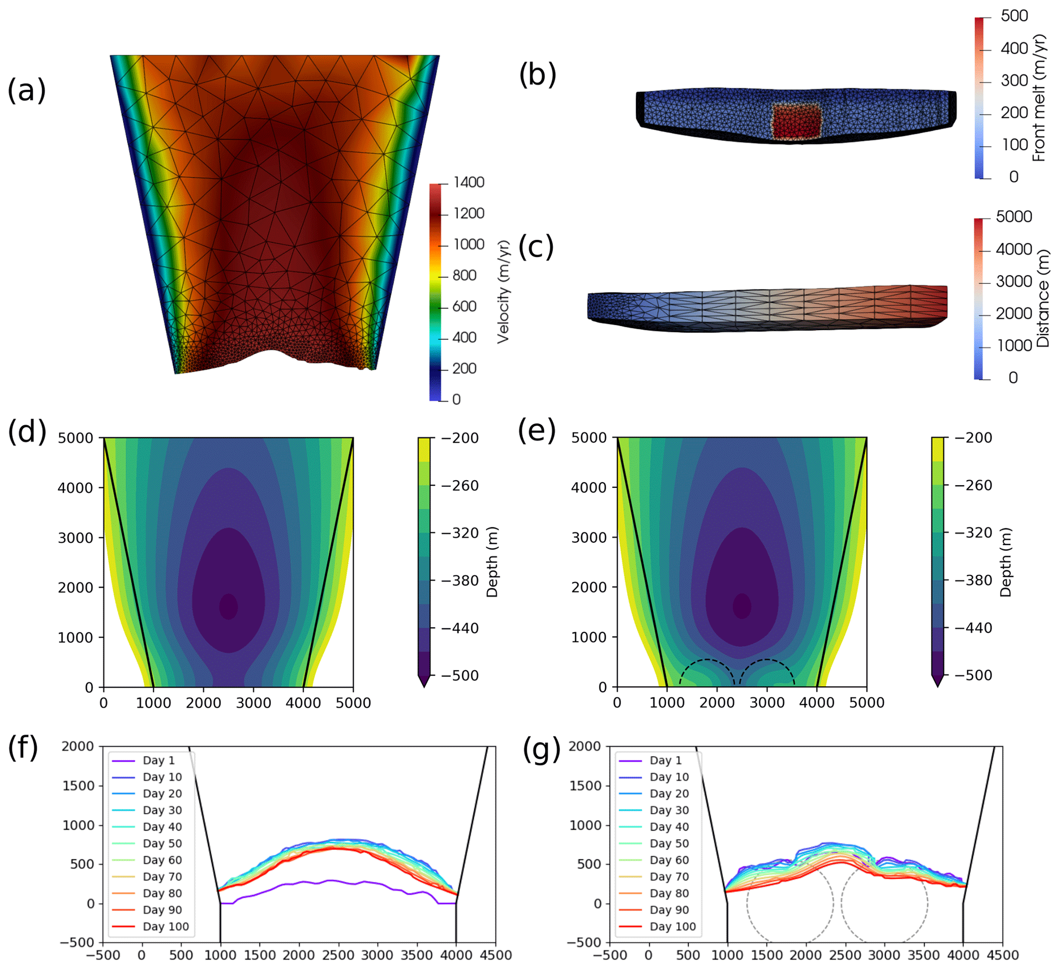
Figure A1The synthetic geometry setup. (a) Top-down view of the mesh at the end of the 100 d simulation with pinning points. Mesh element size is 50 m at the terminus, increasing to 500 m further upstream. The velocity field is displayed. (b) Front view of the same simulation showing the horizontal and vertical element size of 50 m at the terminus. The melt plume can be seen in the centre of the terminus. (c) Side view of the same simulation showing the 50 m mesh density at the terminus and 500 m at the inflow boundary. (d) The bed elevation with no pinning points. (e) The bed elevation with pinning points near the terminus. The terminus evolution of during 100 d simulation with (f) no pinning points and (g) pinning points. The full control simulations for each domain can be seen in Videos 3 and 4 in the Supplement.
A1 Boundary conditions
The synthetic glacier domain had six boundary conditions that consisted of the calving front of the glacier (Γfront), both lateral margins (Γleft,Γright), the interior inflow (Γinflow), the base (Γbase), and the top surface (Γsurf). The boundary conditions applied to each are discussed below.
Since the lateral boundary represents the fjord walls, a no-penetration condition is implemented at the sidewall margins of the model domain. A simple linear friction law, which has a constant slip coefficient (β) of 1 × 10⁻² MPa m−1 a was applied as a Neumann boundary condition. Therefore, the lateral boundary conditions are
where u is the velocity component, σ is the stress component, and the perpendicular and tangential components are shown by ⟂ and , respectively. A non-linear Weertman friction law is applied to the base with a slip coefficient of 1 × 10⁻⁴ and an exponent of 3. The base boundary condition is complicated by the grounding line dynamics of the glacier. The grounding line of the glacier is solved as a contact problem, following Favier et al. (2012). If the glacier is grounded, the boundary condition is similar to the lateral boundary with a non-penetration condition applied as follows:
where C is the Weertman slip coefficient, ub is the basal velocity, and m is the Weertman exponent. If the glacier is ungrounded, no friction is applied, and the glacier is free to move vertically as follows:
where ρw is the density of the water, g is the gravitational acceleration, and h is the depth below the water level. Similar to ungrounded ice, no friction is applied to the glacier-calving face. Since it is in contact with the fjord waterbody, a normal stress is applied below the water level.
The inflow boundary has a fixed velocity of 1000 m yr−1, and this is assumed to be constant throughout the vertical ice column. Therefore, the inflow boundary condition is simply
where u is the velocity vector, and uin is 1000 m yr−1. The surface boundary condition is stress-free, and the surface mass balance is not considered. A submarine melt condition is added to the glacier front boundary or calving front (Γterm) where a central plume is present along with background melt (Fig. A1b). The plume is taken from the summer plumes modelled by Kajanto et al. (2023) at Ilulissat Fjord. The plume profile was then normalised, given the much lower maximum flow velocity at the synthetic geometry of 1500 m yr−1 compared to the much larger speed seen at Jakobshavn Isbræ (> 10 000 m yr−1). Maximal plume melt was set to 500 m yr−1 and the profile adjusted accordingly. No melt was applied to the floating ice on the base.
A2 Ice properties
A constant temperature of −20 °C is set throughout the domain, and the associated ice properties are based on Glen's flow, which is then used to solve the full-Stokes equations (Cuffey and Paterson, 2010). The feedback of the temperature dependency of Glen's flow law is calculated using the Arrhenius equation, and the rate factors are detailed in (Cuffey and Paterson, 2010).
A3 Model solvers and parameters
For the transient simulation, the model is run forward for 100 d at time steps of 1 d, giving a total of 100 time steps. The full-Stokes flow is solved, and from this solution, the Cauchy stress tensor across the domain is computed. Although there are no surface mass balance conditions, the surface and base free surfaces are solved as a kinematic boundary condition so that the glacier can evolve in response to the flow solution. Similarly, the new front advance routines outlined are used to predict the advance of the glacier down the fjord. As a consequence, the mesh is deformed twice, first vertically and then longitudinally. The longitudinal mesh deformation is limited to 1500 m from the calving front of the glacier.
The new calving algorithm as outlined in Sect. 4 is applied, and the front 1500 m of the glacier is remeshed at each time step. The anisotropic remeshing metric had a minimum horizontal resolution of 50 m, which increases to 500 m further inland. It has a constant vertical resolution of 50 m. The adaptive time stepping present in the calving algorithm was active, with a maximum number of added time steps set to three. Time steps were only added if large calving events occurred to capture any consecutive calving from changes in the domain. The calved iceberg threshold was set to 1 × 10⁷ m3 for the adaptive time stepping to be activated. The 2D PlaneMesh that crevasses were mapped onto had a grid size of 40 m.
The crevasse depth (CD) law is modified to make the setup more sensitive to calving and highlight potential numerical influences on calving. This is achieved by reducing the “crevasse penetration threshold” to 92.5 %. Here, full thickness calving occurs when either (1) a surface crevasse penetrates 92.5 % of the ice column between the surface and water line or (2) surface and basal crevasses extend 92.5 % of the entire water column. Although it is known that CD law can underestimate calving (e.g. Choi et al., 2018; Todd et al., 2019; Cook et al., 2023) this should not be concluded in this instance. Instead, the alteration of the calving law should be considered an increase to the sensitivity of a synthetic glacier so that the effects of varying parameters on calving dynamics can be clearly identified in the following simulation tests. No conclusion on the accuracy of the CD law can be made for a synthetic scenario.
In order to distinguish between the any variability arising from the CD law and that of the new calving algorithm, further experiments were run using a simple rate-based law. The new calving law took the following form:
where C is the predicted calving magnitude, Vs is the surface velocity at the terminus, and is the prescribed retreat rate. The prescribed retreat rate is applied normally to the terminus and was set to 1500 m yr−1 for all experiments. The setup excluding the calving law was identical to that described in Appendix A, and the control variables were kept consistent. Complementary experiments to those using the CD law in the main text were run. This produced the mesh density experiments with minimum element sizes of 25, 30, 70, and 100 m. Experiments changing the time step were the same as the main text using time steps of 0.25, 0.33, 0.5, and 2 d. Finally, the use of the adaptive time stepping in the algorithm was set to 0, 1, 5, and 10 d.
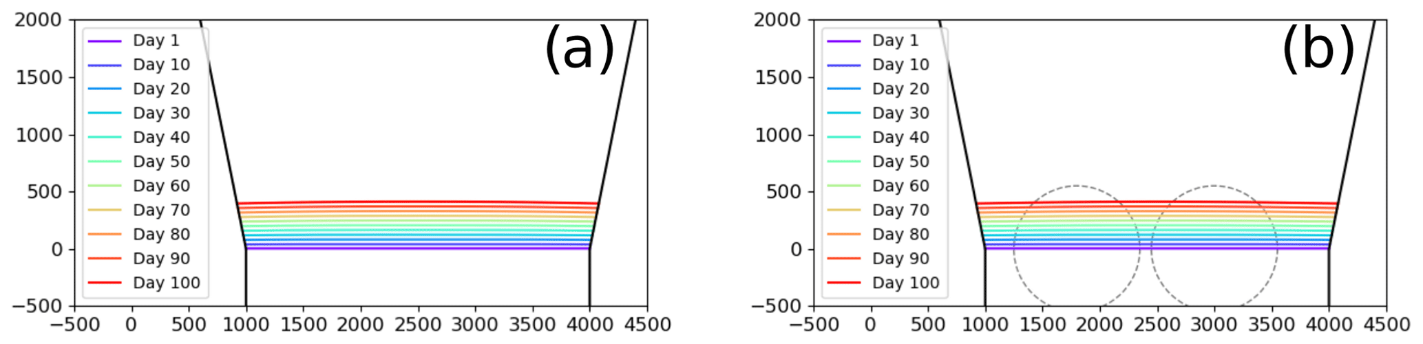
Figure B1Terminus positions through 100 d control experiments using the rate-based law on (a) the domain without pinning points and (b) the domain with pinning points. The outline of the pinning points is shown by the dashed circles. Only the control experiments are shown as the results were too consistent to overlay on each other.
Predicted retreat and calving varied little between the rate-based experiments with a mean of 4.06 m d−1. Maximum and minimum values were only 0.01 m d−1 greater or less than the mean (Table B1). The rate of retreat throughout the experiments was consistent and did not vary between the two different setup domains where the presence of pinning points had no influence on predicted calving (Fig. B1). Simulated retreat was slightly lower than the prescribed R value (4.11 m d−1) but was consistent between experiments.
Table B1Summary of the mean retreat rates for 100 d experiments testing the numerical model parameters using a rate-based calving law. The numerical model parameters tested match those in the main text.
Very little variability in the simulated calving can be attributed to the new calving algorithm, and instead, variability in the main test can be attributed to the CD law. The trivial variation in the rate-based law experiments is due to the Hausdorff distance prescribed in the remeshing, where slight errors are introduced into the surface remapping. It is likely the remeshing is the cause of an insignificant difference between the mean retreat rate and the prescribed retreat rate (0.05 m d−1). However, given the consistency of the implemented retreat, this issue is easily overcome by an adjustment of the input R value.
The data associated with this study are made available in the Supplement. The new algorithm, including current and future releases, is available on the official Elmer/Ice GitHub repository https://github.com/ElmerCSC/elmerfem (last access: 29 July 2024). The exact code used in this study is available on Zenodo at https://doi.org/10.5281/zenodo.10182705 (last access: 29 July 2024) (Wheel, 2023a). The user guides can be accessed from GitHub at https://github.com/ElmerCSC/elmerfem/tree/devel/elmerice/Solvers/Documentation (last access: 29 July 2024). The three documents associated with the new calving algorithm are Calving3D_lset.md, CalvingRemeshMMG.md, and CalvingGlacierAdvance3D.md.
Examples of the glacier advancing at a narrowing and widening fjord are provided in Videos 1 and 2 in the Supplement, respectively. Videos of the control experiment for each domain are provided as Videos 3 and 4 in the Supplement. The supplement related to this article is available online at: https://doi.org/10.5194/gmd-17-5759-2024-supplement.
IW wrote the algorithm with technical support from JT and TZ. IW designed and analysed the experiments with guidance from DB and AC. IW wrote the paper with contributions from DB and AC. All authors contributed and approved the final paper.
The contact author has declared that none of the authors has any competing interests.
Publisher's note: Copernicus Publications remains neutral with regard to jurisdictional claims made in the text, published maps, institutional affiliations, or any other geographical representation in this paper. While Copernicus Publications makes every effort to include appropriate place names, the final responsibility lies with the authors.
This work is from the DOMINOS project, a component of the International Thwaites Glacier Collaboration (ITGC). This work has received support from the Natural Environmental Research Council (NERC; grant no. NE/006605/1) and under the ITGC contribution no. ITGC-116. This research has been supported by the HPC-Europa3 programme, part of the European Union's Horizon 2020 research and innovation programme (grant no. 730897). Thomas Zwinger has been supported by the Finnish Academy COLD consortium (grant no. 322978). We thank the editor, Ludovic Räss, and the reviewers, Gong Cheng and Stephen Cornford, for their helpful comments which greatly improved the paper.
This research has been supported by the Natural Environment Research Council (grant no. NE/S006605/1) and the HORIZON EUROPE European Research Council (grant no. 730897). Thomas Zwinger has been supported by the Finnish Academy COLD consortium (grant no. 322978).
This paper was edited by Ludovic Räss and reviewed by Stephen Cornford and Gong Cheng.
Amaral, T., Bartholomaus, T. C., and Enderlin, E. M.: Evaluation of Iceberg Calving Models Against Observations From Greenland Outlet Glaciers, J. Geophys. Res.-Earth, 125, e2019JF005444, https://doi.org/10.1029/2019JF005444, 2020. a
Åström, J. A., Riikilä, T. I., Tallinen, T., Zwinger, T., Benn, D., Moore, J. C., and Timonen, J.: A particle based simulation model for glacier dynamics, The Cryosphere, 7, 1591–1602, https://doi.org/10.5194/tc-7-1591-2013, 2013. a
Aström, J. A., Vallot, D., Schäfer, M., Welty, E. Z., O'Neel, S., Bartholomaus, T. C., Liu, Y., Riikilä, T. I., Zwinger, T., Timonen, J., and Moore, J. C.: Termini of calving glaciers as self-organized critical systems, Nat. Geosci., 7, 874–878, https://doi.org/10.1038/ngeo2290, 2014. a
Benn, D. I. and Åström, J. A.: Calving glaciers and ice shelves Adv. Phys., 3, 1048–1076, https://doi.org/10.1080/23746149.2018.1513819, 2018. a
Benn, D., Todd, J., Luckman, A., Bevan, S., Chudley, T., Astrom, J., Zwinger, T., Cook, S., and Christoffersen, P.: Controls on calving at a large Greenland tidewater glacier: stress regime, self-organised criticality and the crevasse-depth calving law, J. Glaciol., 1–16, online first, https://doi.org/10.1017/jog.2023.81, 2023. a, b, c, d
Benn, D. I., Hulton, N. R., and Mottram, R. H.: “Calving laws”, “sliding laws” and the stability of tidewater glaciers, in: Annals of Glaciology, Cambridge University Press, vol. 46, 123–130, https://doi.org/10.3189/172756407782871161, 2007. a, b
Benn, D. I., Cowton, T., Todd, J., and Luckman, A.: Glacier Calving in Greenland, Current Climate Change Reports, 3, 282–290, https://doi.org/10.1007/s40641-017-0070-1, 2017. a
Berg, B. and Bassis, J.: Crevasse advection increases glacier calving, J. Glaciol., 68, 977–986, https://doi.org/10.1017/jog.2022.10, 2022. a
Bondzio, J. H., Seroussi, H., Morlighem, M., Kleiner, T., Rückamp, M., Humbert, A., and Larour, E. Y.: Modelling calving front dynamics using a level-set method: application to Jakobshavn Isbræ, West Greenland, The Cryosphere, 10, 497–510, https://doi.org/10.5194/tc-10-497-2016, 2016. a, b, c, d
Choi, Y., Morlighem, M., Wood, M., and Bondzio, J. H.: Comparison of four calving laws to model Greenland outlet glaciers, The Cryosphere, 12, 3735–3746, https://doi.org/10.5194/tc-12-3735-2018, 2018. a
Cook, S. J., Christoffersen, P., Todd, J., Slater, D., and Chauché, N.: Coupled modelling of subglacial hydrology and calving-front melting at Store Glacier, West Greenland, The Cryosphere, 14, 905–924, https://doi.org/10.5194/tc-14-905-2020, 2020. a
Cook, S. J., Christoffersen, P., and Wheel, I.: Coupled 3-D full-Stokes modelling of tidewater glaciers, in: Annals of Glaciology, Cambridge University Press, vol. 63, 1–4, https://doi.org/10.1017/aog.2023.4, 2023. a, b, c, d, e, f, g
Courant, R., Friedrichs, K., and Lewy, H.: Über die partiellen Differenzengleichungen der mathematischen Physik, Math. Ann., 100, 32–74, https://doi.org/10.1007/BF01448839, 1928. a
Cuffey, K. and Paterson, W.: The physics of glaciers, 4th Edn., Academic Press, ISBN 9780123694614., 2010. a, b
Dapogny, C., Dobrzynski, C., and Frey, P.: Three-dimensional adaptive domain remeshing, implicit domain meshing, and applications to free and moving boundary problems, J. Comput. Phys., 262, 358–378, https://doi.org/10.1016/j.jcp.2014.01.005, 2014. a, b
Devine, K. D., Boman, E. G., Riesen, L. A., Catalyurek, U. V., and Chevalier, C.: Getting Started with Zoltan: a Short Tutorial, Tech. rep., Sandia National Laboratories, Albuquerque, USA, https://sandialabs.github.io/Zoltan//papers/Dagstuhl09.pdf (last access: 29 September 2024), 2009. a
Durand, G., Gagliardini, O., De Fleurian, B., Zwinger, T., and Le Meur, E.: Marine ice sheet dynamics: Hysteresis and neutral equilibrium, J. Geophys. Res.-Sol. Ea., 114, F03009, https://doi.org/10.1029/2008JF001170, 2009. a, b
Favier, L., Gagliardini, O., Durand, G., and Zwinger, T.: A three-dimensional full Stokes model of the grounding line dynamics: Effect of a pinning point beneath the ice shelf, The Cryosphere, 6, 101–112, https://doi.org/10.5194/tc-6-101-2012, 2012. a
Gagliardini, O., Zwinger, T., Gillet-Chaulet, F., Durand, G., Favier, L., de Fleurian, B., Greve, R., Malinen, M., Martín, C., Råback, P., Ruokolainen, J., Sacchettini, M., Schäfer, M., Seddik, H., and Thies, J.: Capabilities and performance of Elmer/Ice, a new-generation ice sheet model, Geosci. Model Dev., 6, 1299–1318, https://doi.org/10.5194/gmd-6-1299-2013, 2013. a
Gillet-Chaulet, F., Gagliardini, O., Seddik, H., Nodet, M., Durand, G., Ritz, C., Zwinger, T., Greve, R., and Vaughan, D. G.: Greenland ice sheet contribution to sea-level rise from a new-generation ice-sheet model, The Cryosphere, 6, 1561–1576, https://doi.org/10.5194/tc-6-1561-2012, 2012. a
IPCC: IPCC, 2023: Summary for Policymakers, in: Climate Change 2023: Synthesis Report. A Report of the Intergovernmental Panel on Climate Change. Contribution of Working Groups I, II and III to the Sixth Assessment Report of the Intergovernmental Panel on Climate Change, edited by: Lee, H. and Romero, J., IPCC, Geneva, Switzerland, 2023. a
Joughin, I., Shean, D. E., Smith, B. E., and Floricioiu, D.: A decade of variability on Jakobshavn Isbræ: ocean temperatures pace speed through influence on mélange rigidity, The Cryosphere, 14, 211–227, https://doi.org/10.5194/tc-14-211-2020, 2020. a
Kajanto, K., Straneo, F., and Nisancioglu, K.: Impact of icebergs on the seasonal submarine melt of Sermeq Kujalleq, The Cryosphere, 17, 371–390, https://doi.org/10.5194/tc-17-371-2023, 2023. a
Nick, F. M., Van Der Veen, C. J., Vieli, A., and Benn, D. I.: A physically based calving model applied to marine outlet glaciers and implications for the glacier dynamics, J. Glaciol., 56, 781–794, https://doi.org/10.3189/002214310794457344, 2010. a, b
Nye, J. F.: The distribution of stress and velocity in glaciers and ice-sheets, P. Roy. Soc. Lond. A Mat., 239, 113–133, https://doi.org/10.1098/rspa.1957.0026, 1957. a
O'Leary, M. and Christoffersen, P.: Calving on tidewater glaciers amplified by submarine frontal melting, The Cryosphere, 7, 119–128, https://doi.org/10.5194/tc-7-119-2013, 2013. a
Osher, S. and Fedkiw, R. P.: Level Set Methods: An Overview and Some Recent Results, J. Comput. Phys., 169, 463–502, https://doi.org/10.1006/jcph.2000.6636, 2001. a, b, c
Scambos, T. A., Bell, R. E., Alley, R. B., Anandakrishnan, S., Bromwich, D. H., Brunt, K., Christianson, K., Creyts, T., Das, S. B., DeConto, R., Dutrieux, P., Fricker, H. A., Holland, D., MacGregor, J., Medley, B., Nicolas, J. P., Pollard, D., Siegfried, M. R., Smith, A. M., Steig, E. J., Trusel, L. D., Vaughan, D. G., and Yager, P. L.: How much, how fast?: A science review and outlook for research on the instability of Antarctica's Thwaites Glacier in the 21st century, Global Planet. Change, 153, 16–34, https://doi.org/10.1016/j.gloplacha.2017.04.008, 2017. a
Sethian, J. A.: Level set methods and fast marching methods, 2nd Edn., Cambridge University Press, ISBN 9780521645577, 1999. a, b, c
Slater, D., Nienow, P., Sole, A., Cowton, T., Mottram, R., Langen, P., and Mair, D.: Spatially distributed runoff at the grounding line of a large Greenlandic tidewater glacier inferred from plume modelling, J. Glaciol., 63, 309–323, https://doi.org/10.1017/jog.2016.139, 2017. a
Todd, J. and Christoffersen, P.: Are seasonal calving dynamics forced by buttressing from ice mélange or undercutting by melting? Outcomes from full-Stokes simulations of Store Glacier, West Greenland, The Cryosphere, 8, 2353–2365, https://doi.org/10.5194/tc-8-2353-2014, 2014. a
Todd, J., Christoffersen, P., Zwinger, T., Råback, P., Chauché, N., Benn, D., Luckman, A., Ryan, J., Toberg, N., Slater, D., and Hubbard, A.: A Full-Stokes 3-D Calving Model Applied to a Large Greenlandic Glacier, J. Geophys. Res.-Earth, 123, 410–432, https://doi.org/10.1002/2017JF004349, 2018. a, b, c, d, e, f, g, h, i, j
Todd, J., Christoffersen, P., Zwinger, T., Råback, P., and Benn, D. I.: Sensitivity of a calving glacier to ice–ocean interactions under climate change: new insights from a 3-D full-Stokes model, The Cryosphere, 13, 1681–1694, https://doi.org/10.5194/tc-13-1681-2019, 2019. a, b, c, d, e, f, g, h
Van Dongen, E., Jouvet, G., Walter, A., Todd, J., Zwinger, T., Asaji, I., Sugiyama, S., Walter, F., and Funk, M.: Tides modulate crevasse opening prior to a major calving event at Bowdoin Glacier, Northwest Greenland, J. Glaciol., 66, 113–123, https://doi.org/10.1017/jog.2019.89, 2019. a
van Dongen, E. C., Åström, J. A., Jouvet, G., Todd, J., Benn, D. I., and Funk, M.: Numerical Modeling Shows Increased Fracturing Due to Melt-Undercutting Prior to Major Calving at Bowdoin Glacier, Front. Earth Sci., 8, 1–12, https://doi.org/10.3389/feart.2020.00253, 2020. a
Wheel, I.: StAndrewsGlacio/ElmerIceCalvingModel: 3D Calving Model in Elmer/Ice (v9.0), Zenodo [code], https://doi.org/10.5281/zenodo.10182705, 2023a. a, b
Wheel, I.: Algorithm outline associated with the 3D full-Stokes calving model in Elmer/Ice (v9.0) associated with EGUSPHERE-2023-2778, Zenodo [code], https://doi.org/10.5281/zenodo.10182710, 2023b. a
- Abstract
- Introduction
- Modelling calving in a continuum
- Implementation of calving in a continuum model
- The new calving algorithm: methods and capabilities
- Typical simulation
- Model parameter experiments
- Summary of a model capabilities and potential
- Conclusions
- Appendix A: Synthetic glacier setup
- Appendix B: Rate-based calving law experiments
- Code and data availability
- Author contributions
- Competing interests
- Disclaimer
- Acknowledgements
- Financial support
- Review statement
- References
- Supplement