Evaluation of the coupling of EMACv2.55 to the land surface and vegetation model JSBACHv4

We present the coupling of the Jena Scheme for Biosphere–Atmosphere Coupling in Hamburg version 4 (JSBACHv4) to the ECHAM/MESSy Atmospheric Chemistry (EMAC) model. With JSBACH, the soil water bucket model in EMAC is replaced by a diffusive hydrological transport model for soil water that includes water storage and infiltration in five soil layers, preventing soil from drying too rapidly and reducing biases in soil temperature and moisture. A three-layer soil scheme is implemented, and phase changes in water in the soil are considered. The leaf area index (LAI) climatology in EMAC has been substituted with a phenology module calculating the LAI. Multiple land cover types are included to provide a state-dependent surface albedo, which accounts for the absorption of solar radiation by vegetation. Plant net primary productivity, leaf area index and surface roughness are calculated according to the plant functional types. This paper provides a detailed evaluation of the new coupled model based on observations and reanalysis data, including ERA5/ERA5-Land datasets, Global Precipitation Climatology Project (GPCP) data and Moderate Resolution Imaging Spectroradiometer (MODIS) satellite data. Land surface temperature (LST), terrestrial water storage (TWS), surface albedo (α), net top-of-atmosphere radiation flux (Rad_TOA), precipitation (precip), leaf area index (LAI), fraction of absorbed photosynthetic active radiation (FAPAR) and gross primary productivity (GPP) are evaluated in particular. The strongest correlation (r) between reanalysis data and the newly coupled model is found for LST (r=0.985, with an average global bias of −1.546 K), α (r=0.947, with an average global bias of −0.015) and Rad_TOA (r=0.907, with an average global bias of 3.56 W m⁻²). Precipitation exhibits a correlation with the GPCP dataset of 0.523 and an average global bias of 0.042 mm d⁻¹. The LAI optimisation yields a correlation of 0.637 with observations and a global mean deviation of −0.212. FAPAR and GPP exemplify two of the many additional variables made available through JSBACH in EMAC. FAPAR and observations show a correlation of 0.663, with an average global difference of −0.223, while the correlation for GPP and observations is 0.564 and the average global difference is −0.001 kg carbon km⁻¹. Benefiting from the numerous added features within the simulated land system, the representation of soil moisture is improved, which is critical for vegetation modelling. This improvement can be attributed to a general increase in soil moisture and water storage in deeper soil layers and a closer alignment of simulated TWS with observations, mitigating the previously widespread problem of soil drought. We show that the numerous newly added components strongly improve the land surface, e.g. soil moisture, TWS and LAI, while surface parameters, such as LST, surface albedo or Rad_TOA, which were mostly prescribed according to climatologies, remain similar. The coupling of JSBACH brings EMAC a step closer towards a holistic comprehensive Earth system model and extends its versatility.

1 Introduction

Earth system models (ESMs) are needed to analyse current and future climate scenarios, and particularly in view of ongoing climate change (IPCC, 2021), it is crucial to include the main Earth system components to identify and quantify potential feedback mechanisms. These numerical models are based on a mathematical formulation of the physical and chemical processes, accounting for interactions between the atmosphere, oceans and biogeochemical processes on land (Flato, 2011). Common ESMs contain an atmospheric general circulation model (A-GCM), an ocean general circulation model (O-GCM) and a land surface model (LSM). A comprehensive list of existing ESMs can be found, for instance, in “Annex II: Models” of the Sixth Assessment Report of the Intergovernmental Panel on Climate Change (Gutiérrez et al., 2021).

The ECHAM5/MESSy Atmospheric Chemistry (EMAC) general circulation model is based on an underlying A-GCM; more specifically, the spectral dynamical core, the large-scale advection and the “nudging” method are originally from ECHAM5 (the fifth generation of the European Centre HAMburg general circulation model; Roeckner et al., 2006). The physical parameterisations from ECHAM have been modularized between respective further-developed MESSy submodels. These include a simplified surface model (SURFACE); O-GCM MPIOM (Pozzer et al., 2011a); and several other submodels which address atmospheric chemistry, cloud and transport processes (Roeckner et al., 2003; Jöckel et al., 2005, 2010). The coupling is achieved via the Modular Earth Submodel System (MESSy2) framework, gradually refined and expanded during the past 2 decades to provide an infrastructure of submodel and process combinations with a wide range of applications. EMAC is a community model with a growing number of users contributing to developments in various research areas, e.g. studies on particle concentrations and aerosols (Kohl et al., 2023; Righi et al., 2023), oxidation capacity (Nussbaumer et al., 2023; Friedel et al., 2023), atmospheric dynamics (Eichinger et al., 2023; Charlesworth et al., 2023) and environmental consequences for human health (Pozzer et al., 2023; Milner et al., 2023). Furthermore, an alternative dynamic vegetation scheme (LPJ-GUESS; Forrest et al., 2020) has been coupled to EMAC, allowing for climate–vegetation interactions (e.g. Vella et al., 2023b). In the following, the implementation and evaluation of the LSM Jena Scheme for Biosphere–Atmosphere Coupling in Hamburg (JSBACH), a substitute of EMAC's current surface model, is documented. JSBACH is implemented into the MESSy framework following the relevant coding standards. The dynamical land–surface model JSBACH was first developed as the land model for ECHAM at the Max Planck Institute for Meteorology (MPI-M) (Reick et al., 2021). Originally, it emerged from the combination of all ECHAM5 land processes in a separate land model and was further developed and refined, now providing a large repertoire of biogeochemical processes of the ecosystem. The latest version (JSBACHv4) is part of the Icosahedral Nonhydrostatic Land (ICON-Land) model and has not yet been coupled to models simulating atmospheric chemistry (Pham et al., 2021).

The implementation of JSBACH represents significant progress in the development of the ESM EMAC. As climate change progresses and the occurrence of extreme weather events increases, the influence of surface processes and vegetation becomes more prominent (Domeisen et al., 2022). Vegetation and soil water balance are the driving factors for surface fluxes of heat and moisture, affecting temperature, precipitation, atmospheric dynamics and chemistry (Miralles et al., 2019; Lauwaet et al., 2009; Matyssek et al., 2014; Mellouki et al., 2015). JSBACH replaces the soil water bucket model included in the MESSy submodel SURFACE by a more comprehensive five-layer hydrological soil model. This substitution aims at improving the representation of surface energy fluxes of heat and moisture, reducing biases in surface temperature and subsequent plant stress and their impact on biogenic emissions. JSBACH enables the analysis of biogeochemical processes on much smaller timescales, including not only climatic scales, but also days and hours. This allows for the analysis of the impact of vegetation on atmospheric chemistry, plant stomatal uptake, volatile organic compound (VOC) emissions and associated feedback mechanisms and enables a more detailed understanding of land–atmosphere interactions. Furthermore, the impact on the surface energy budget allows for a more consistent representation of chemical and transport processes in the atmospheric boundary layer. In Sect. 2, we give a short description of JSBACH and describe the coupling of EMAC and JSBACH via MESSy, including the tuning of the newly coupled model. In Sect. 3, the evaluation variables and corresponding observation and reanalysis datasets are introduced. The results and the discussion of the corresponding evaluation are presented in Sect. 4.

2 Model description

2.1 JSBACH

In this work, we implemented the most recent version of JSBACH (JSBACHv4, Schneck et al., 2022). A detailed description of the parameterisations used in JSBACH can be found in Reick et al. (2013, 2021), while Schneck et al. (2022) present features of the version JSBACHv4 in comparison with the previous one (JSBACHv3) along with an assessment of the results of both versions. On the technical side, JSBACHv4 has been improved with modernised source codes and software infrastructure, while on the application side, it offers an improved soil scheme with a dynamic calculation of ground heat conductivity and capacity, taking phase change in water and organic fractions within soil layers into account (Jungclaus et al., 2022; Schneck et al., 2022; Ekici et al., 2014). It provides a complex soil hydrological transport model that includes percolation and storage of water in several soil depths, reaching down to 9.8 m with increasing layer thickness of 0.065, 0.254, 0.913, 2.902 and 5.7 m for the first to the fifth layer, respectively. This gives a realistic estimate of soil desiccation and corresponding soil temperature and moisture. Additionally, the new version introduces a fractional lake mask, a three-layer snow scheme and the forest age structures (Schneck et al., 2022; de Vrese et al., 2021; Nabel et al., 2020). The implemented version of JSBACHv4 does not include the natural vegetation dynamics, land-use transitions and nitrogen cycle from JSBACH3. Those mechanisms have only recently been adopted in JSBACHv4 and will be added to MESSy in the near future. However, on the climate timescale, the interactions between climate and vegetation are already available in MESSy through the LPJ-GUESS interactive vegetation module (Vella et al., 2023a).

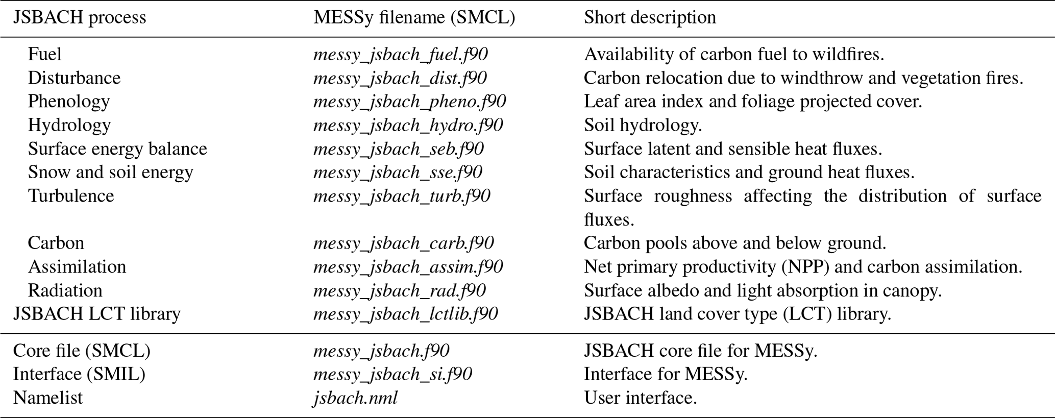
In the case of the ICON-Land infrastructure, a clear separation of the physical processes used in JSBACHv4 is allowed. The processes used in this study include the vegetation coverage, phenology and plant productivity (defined via gross primary productivity, GPP, and net primary productivity, NPP, and photosynthesis); a turbulence and radiation scheme; surface energy balance; and the exchange fluxes of heat and moisture, soil and vegetation carbon turnover, and disturbances due to wildfires or windthrow. The processes are listed in Table 1. In JSBACH, subgrid-scale heterogeneity is taken into account by a tile approach; i.e. grid boxes are divided into tiles associated with a specific land cover type (Reick et al., 2021). All available land cover types are listed in Table A1. The concept allows us to define processes specific to the different land cover types. For example, processes only related to vegetation (such as photosynthesis) are calculated only on vegetated tiles. Based on Reick et al. (2021), water, carbon, nitrogen, and area are conserved with numerical accuracy. Energy conversion is not fully achieved yet since the temperature of rainwater and heat produced by heterotrophic respiration are not accounted for (Reick et al., 2013, 2021).

To couple JSBACH with EMAC, it is implemented as a new submodel within the MESSy framework, following its well-described coding standards (Jöckel et al., 2010). Each process of the JSBACHv4 source code (listed in Table 1) is implemented as an individual Fortran module in the MESSy submodel core layer (SMCL) and complemented by a newly created submodel core layer file. A schematic overview of JSBACH as a new submodel in EMAC and corresponding process calls are given in the Supplement. In addition to the individual JSBACH processes, the file “messy_jsbach.f90” is created, which includes the definitions of land-cover specifications (originally taken from lctlib_nlct21.def), the tile aggregation subroutines and the subroutine to read the JSBACH namelist. The namelist (jsbach.nml) serves as a user interface, where input and coupling variables are specified. The full namelist is available in the Supplement; the coupled variables are listed from line 152 to 206 of the namelist. Parameters can be defined, and logical switches to modify and adjust the simulation can be set. The module subroutines are called from a newly created JSBACH interface (messy_jsbach_si.f90), which is implemented in the MESSy submodel interface layer (SMIL). Besides the process calls, the interface includes the creation of new “representations” to expand the EMAC model grid to new dimensions, for soil, snow and canopy layers and vegetation tiles, and the JSBACH output variables are saved as new “channel objects”. Both representations and channel objects are elements defined in the submodel CHANNEL, which handles the memory, data output (including checkpointing) and internal data exchange (Jöckel et al., 2010).

JSBACH was chosen as the LSM for EMAC since it has already been successfully implemented and tested in other models like the Icosahedral Nonhydrostatic Earth System Model (ICON-ESM) and its predecessor (JSBACH3) in the Max Planck Institute Earth System Model, MPI-ESM 1.2 (Mauritsen et al., 2019), which took part in the Coupled Model Intercomparison Project phases 5 and 6 (Giorgetta et al., 2013). Furthermore, in JSBACH, specific ecosystem processes, like carbon cycling, are included. Those mechanisms will, in combination with an atmospheric chemistry model, provide new and interesting insights into the interactions and feedback mechanisms between vegetation and atmospheric composition. The combination of EMAC and JSBACH makes it possible to analyse biogeochemical processes at various spatial and temporal resolutions, from small-scale experiments of local sub-daily effects to global-scale climate change experiments, in contrast to the coupling of the dynamic vegetation model LPJ-GUESS to EMAC (Forrest et al., 2020), in which the vegetation–atmosphere coupling is restricted by the diurnal time step of the vegetation scheme.

Table 1 JSBACH file overview.

2.2 The EMAC model

The ECHAM/MESSy Atmospheric Chemistry (EMAC) model is a numerical chemistry and climate simulation system that includes submodels describing tropospheric and middle-atmosphere processes and their interaction with oceans, land and human influences (Jöckel et al., 2010). It uses the second version of the Modular Earth Submodel System (MESSy2) to link multi-institutional computer codes. The core atmospheric model is the fifth-generation European Centre Hamburg general circulation model (ECHAM5; Roeckner et al., 2006). The physics subroutines of the original ECHAM code have been modularised and reimplemented as MESSy submodels and have continuously been further developed. Only the spectral transform core, the flux-form semi-Lagrangian large-scale advection scheme, and the nudging routines for Newtonian relaxation remain from ECHAM. Further details on EMAC are documented by Jöckel et al. (2016) and can be found on the MESSy website (https://www.messy-interace.org, last access: 12 October 2023).

2.3 Parameter optimisation

JSBACH is an alternative to the standard submodel used, SURFACE. In the case JSBACH is used, the SURFACE submodel must be switched off. Using JSBACH, a more complex scheme for land temperature and hydrology is adopted, and with that, the dynamical lower-boundary conditions of ECHAM5 are modified. Since the EMAC dynamics were optimised for the specific combination of ECHAM5 and SURFACE (Kern, 2013), the new combination of ECHAM5 and JSBACH requires a refined parameter optimisation (“re-tuning”), with respect to radiation balance, land surface temperature and clouds. Such a parameter optimisation is generally performed to adjust the model results to be as close as possible to observations and to prevent the model climate from drifting, for example, due to a large radiative imbalance. It is achieved by small variations in specific parameters for processes with a high degree of uncertainty or a high level of parameterisation, such as the ones related to clouds and convection. A more detailed description of the optimisation process is provided by Mauritsen et al. (2012). The five parameters optimised in this study are the correction factor for asymmetries of ice clouds (zasic), the homogeneity factors for ice and liquid water clouds (zinhomi and zinhoml), the convective mass flux at the level of neutral buoyancy (cmfctop), and the conversion factor from cloud water to rain (cprcon; in s² m⁻²). Simulations for the same period from 1990 to 2010 were carried out with gradually changing parameters. The simulation using JSBACH based on the default parameters is from now on referred to as CTRL. The climatically optimised simulation is from here on referred to as EMAC/JSBACH, while the simulation without JSBACH (and with SURFACE activated instead) is referred to as EMAC/SRF. The simulations with the according parameter setups are listed in Table S2 in the Supplement (simulations 2 and 31 were not completed due to server failures and were excluded from the analysis). Subsequently, the global and temporal averages of LST; top-of-atmosphere (TOA); and surface (SRF) radiation including net, solar and terrestrial parts; heat flux including net, sensible and latent parts; total column fractional cloud coverage; total column cloud liquid and ice water content; and TWS are calculated and compared to ERA5 and ERA5-Land monthly averaged data (Muñoz Sabater, 2019). Additionally, the global and temporal average of precipitation is compared to the Global Precipitation Climatology Project (GPCP) monthly precipitation dataset (Adler et al., 2003). These datasets are from here on referred to as reference data REF. The results of the global and time averages of the previously mentioned parameters for each simulation are listed in Table S3 in the Supplement. The corresponding RMSE and NRMSE (RMSE normalised by the range of the reference data) are shown in Table S4 in the Supplement. The criteria used for the selection of the optimised tuning parameters were, on the one hand, the smallest deviation from the reference data paired with the lowest normalised root mean square error (NRMSE) sum and, on the other hand, the change in as few parameters as possible to stay as close as possible to the tuning of EMAC/SURF. The sets of parameters of CTRL and EMAC/JSBACH are listed in Table 2. As shown here, only one parameter needed to be adjusted via the replacement of the calculation of zinhoml dependent on model level (lev) and liquid water path (lwp) by a constant value of 0.92. The default value of zinhoml is calculated based on Eqs. (11.52)–(11.53) in Roeckner et al. (2003), viz.

$$\begin{array}{}\text{(1)}& \begin{array}{rl}& {\mathrm{zinhoml}}_{\mathrm{default}}=\\ & \left\{\begin{array}{ll}({\sum }_{\mathrm{0}}^{\mathrm{nlev}}\mathrm{lwp}\partial \mathrm{lev}{)}^{-\mathrm{0.1}}& \text{if }({\sum }_{\mathrm{0}}^{\mathrm{nlev}}\mathrm{lwp}\partial \mathrm{lev})>\mathrm{1},\\ \mathrm{1}& \text{otherwise},\end{array}\right.\end{array}\end{array}$$

with nlev being the number of model levels.

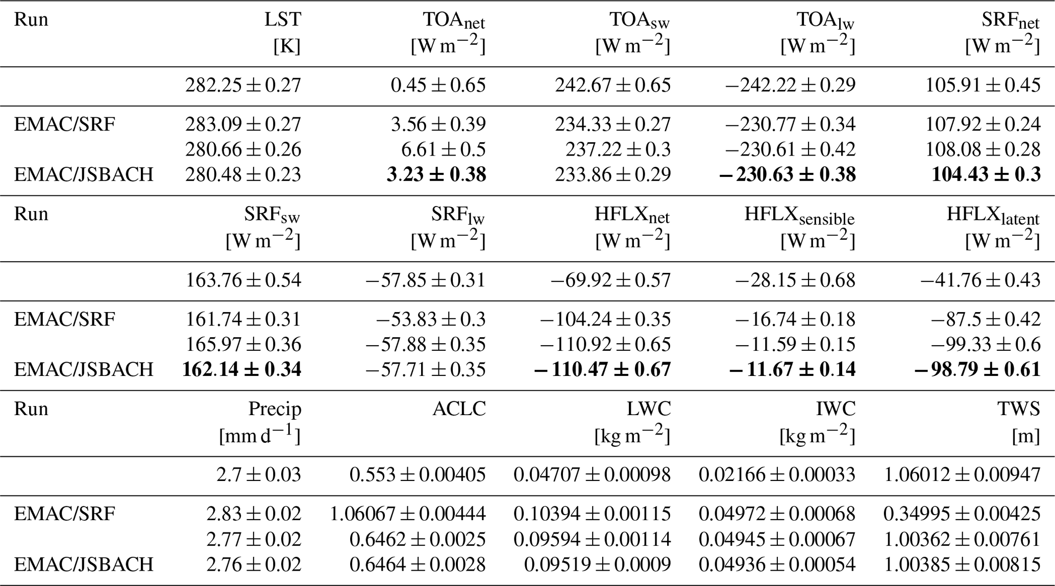
The temporally and spatially averaged results of REF, EMAC/SRF, CTRL and EMAC/JSBACH are shown in Table 3, with values that could be improved with respect to CTRL indicated in bold.

Table 2 List of the optimised parameters of the simulation without JSBACH (EMAC/SRF), the control simulation including JSBACH (CTRL) and the simulation best fitting the requirements (EMAC/JSBACH).

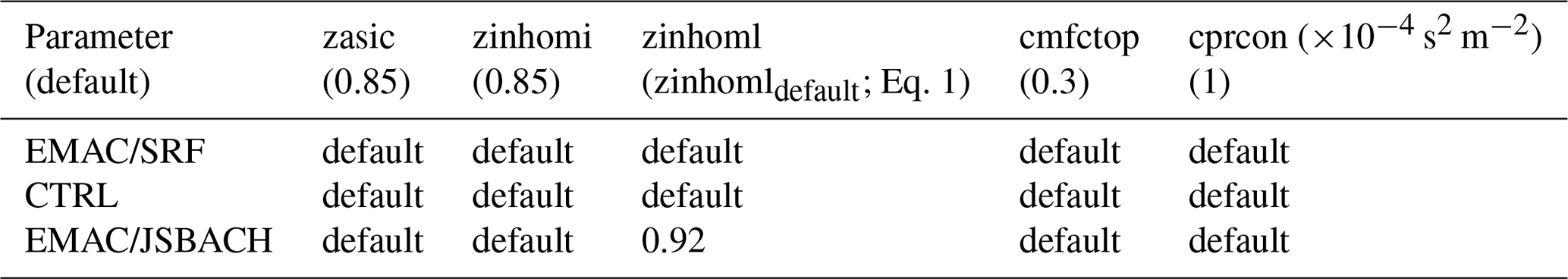
Table 3 Table of the temporally and globally averaged results, with inter-annual variability as the standard deviation of CTRL, EMAC/SRF and EMAC/JSBACH from 1990 to 2010. The corresponding reanalysis or observational results are listed as REF. For precipitation, REF refers to the GPCP monthly precipitation dataset (Adler et al., 2003), while for the remaining variables, REF refers to ERA5 and ERA5-Land reanalysis datasets (Hersbach, 2023; Muñoz Sabater, 2019, 2021). TOA_net refers to the sum of shortwave (TOA_sw) and longwave (TOA_lw) top-of-atmosphere radiation flux, while SRF_* refers to the same at surface level. HFLX_net refers to the sum of the sensible (HFLX_sensible) and latent (HFLX_latent) heat fluxes. Clouds are assessed based on the accumulated cloud cover (ACLC), the liquid water content (LWC) and the ice water content in clouds (IWC).

3 Evaluation

3.1 Model setup

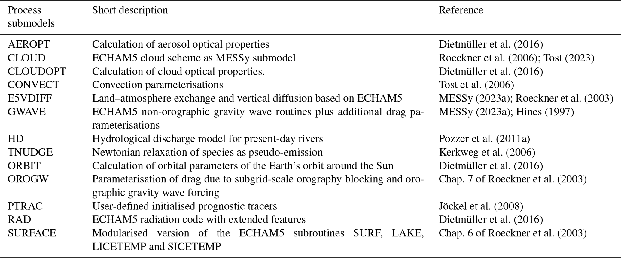
For the present study, we applied EMAC (MESSy version 2.55.0) at the T63L31ECMWF resolution, i.e. with a spherical truncation of T63 (corresponding to a quadratic Gaussian grid of approx. 1.8° by 1.8° spacing in latitude and longitude), with 31 vertical hybrid pressure levels up to 10 hPa. An overview of the submodels used in the reference simulation EMAC/SRF is given in Table 4 along with a brief description of each. In the simulation EMAC/JSBACH, the submodel SURFACE is replaced by the new submodel, JSBACH, and the tuning parameters are updated, while the remaining setup is unchanged. Both simulations were performed from January 1970 to January 2011 and include tracer nudging of CO₂, CH₄, N₂O, CFC11 and CFC12 based on tracer profiles derived from Atmospheric Chemistry and Climate Model Intercomparison Project (ACCMIP) historical lower-boundary condition datasets (Lamarque et al., 2010, 2013). JSBACH is operated on three snow layers, three canopy layers and five soil layers, reaching a depth of 9.8 m below the surface. From 21 possible land cover types (LCTs), 11 plant functional types (PFTs) are taken into account for the standard tile setup (Table A1 in the Appendix). Those are tropical and extratropical broadleaf evergreen and deciduous trees, raingreen shrubs, deciduous shrubs, C₃ and C₄ grass, C₃ and C₄ pasture, and C₃ and C₄ crops. This evaluation focuses only on the dynamical coupling between EMAC and JSBACH; thus, all calculations of atmospheric chemistry and the O-GCM are deactivated. Aerosol concentrations are prescribed for all simulations based on Tanré et al. (1997). A list of all coupled variables can be found in the namelist attached in the electronic Supplement. Coupled variables include surface temperature, latent and sensible fluxes, ground heat fluxes, soil water content, surface albedo, and specific humidity at the lowest atmospheric level. Atmospheric Model Intercomparison Project (AMIP)-type simulations were performed with prescribed monthly sea surface temperature and sea ice concentration to identify systematic errors in the model (Gates et al., 1999). The sea surface temperature and ice concentration are based on ERA5 6-hourly data from 1940 to present (Hersbach et al., 2020) and are the same for all performed simulations. JSBACH was initialised with carbon pool, soil and land property data from the year 2005 (in the Supplement), which are estimated to stabilise within 5 years. This is possible since we perform AMIP-type simulations in which the land–carbon interaction remains inactive. Atmospheric variables stabilise within days, and the soil moisture is estimated to be the slowest variable to adjust to equilibrium, with a maximum adjustment time of 1 year (Hagemann and Stacke, 2015; Schneck et al., 2022). Therefore, the first year (1970) is considered the spin-up time and is not taken into account for the evaluation.

Dietmüller et al. (2016)Roeckner et al. (2006); Tost (2023)Dietmüller et al. (2016)Tost et al. (2006)MESSy (2023a); Roeckner et al. (2003)MESSy (2023a); Hines (1997)Pozzer et al. (2011a)Kerkweg et al. (2006)Dietmüller et al. (2016)Roeckner et al. (2003)Jöckel et al. (2008)Dietmüller et al. (2016)Roeckner et al. (2003)

Table 4 List of the submodels comprising the EMAC/SRF simulation including short description and reference.

3.1.1 Evaluation variables and reference datasets

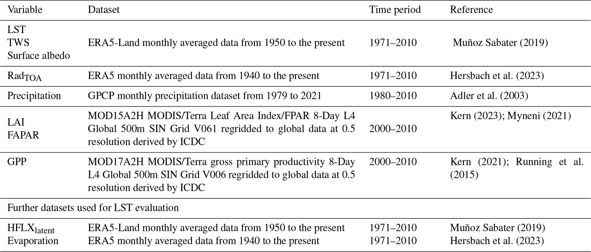
The selected variables to be assessed are variables representing not only the land surface, like land surface temperature (LST), terrestrial water storage (TWS) and surface albedo (α), but also other atmospheric variables, like precipitation (precip), top-of-atmosphere radiation balance (Rad_TOA), fraction of absorbed photosynthetic active radiation (FAPAR), leaf area index (LAI) and gross primary productivity (GPP), in line with the study of Schneck et al. (2022). These variables are compared either to ERA5/ERA5-Land reanalysis datasets or directly to observational datasets of the GPCP or MODIS satellite data (Table 5). The ERA5/ERA-Land reanalysis data are a combination of synthesised estimates of the climate state, which are calculated based on as many observations as possible, and a numerical model due to either direct assimilation of the observations or forcings (Muñoz Sabater, 2019). A comprehensive overview of the limitations and uncertainties in the MODIS data is provided by Disney et al. (2016). The MODIS standard deviations of LAI, FAPAR and GPP are displayed in the Appendix (Figs. A2, A3 and A4) together with the GPCP precipitation error (Fig. A1).

Muñoz Sabater (2019)Hersbach et al. (2023)Adler et al. (2003)Kern (2023)Myneni (2021)Kern (2021)Running et al. (2015)Muñoz Sabater (2019)Hersbach et al. (2023)

Table 5 Table of the evaluation variables, the corresponding reference dataset and the time period of the evaluation analysed.

4 Results and discussion

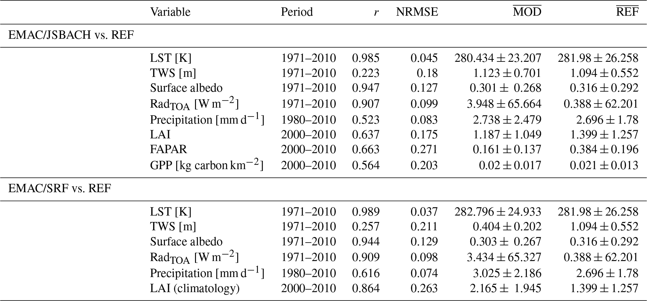
To get an overview of the model performance compared to the reference data, their statistical metrics of the monthly and globally averaged results are presented in Fig. 1 as a Taylor diagram (Taylor, 2001). For the classification of the results of the coupled model, the statistical measures of the model results without the coupling to JSBACH are added. Results of the EMAC/JSBACH are shown as dots, while the results of the EMAC/SRF simulation are displayed as crosses. The Taylor plot shows the Pearson correlation coefficient between simulated and reference data on straight lines stemming from the origin, with arcs around the origin indicating the standard deviation normalised by the reference standard deviation and arcs around the value of 1 indicating the root mean square error normalised by the range of the reference data (NRMSE). The Pearson correlation coefficient (r) and NRMSE are listed in Table 6, together with the weighted global average, with standard deviations for the model simulations ($\stackrel{\mathrm{‾}}{\mathrm{MOD}}$) and reference data ($\stackrel{\mathrm{‾}}{\mathrm{REF}}$). The correlation and NRMSE are based on monthly averages for the available time period of the reference datasets, with the correlation conducted over time and location (see Table 6). This covers the years 1971–2010 for LST, Rad_TOA, α and TWS. Precipitation is analysed for the period 1980–2010 and LAI, FAPAR and GPP for 2000–2010.

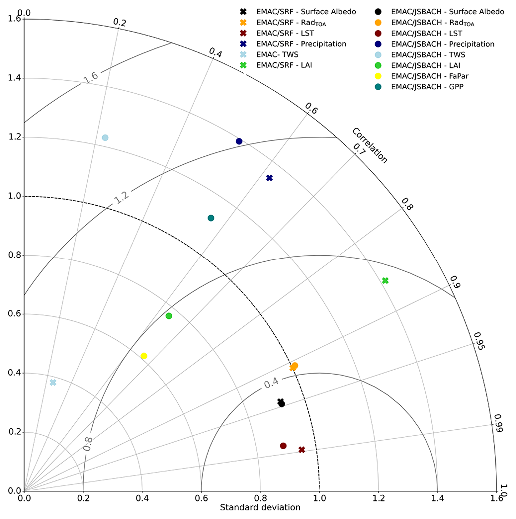
Figure 1 Taylor plots of the Pearson correlation coefficient; root mean square error (RMSE); and standard deviation normalised with the reference data standard deviation of monthly means of LST (1971–2010), Rad_TOA (1971–2010), surface albedo (1971–2010), precipitation (1980–2010), TWS (1971–2010), LAI (2000–2010), FAPAR (2000–2010) and GPP (2000–2010). The statistical measures of the EMAC/JSBACH are displayed as dots, while the EMAC/SRF values are shown as crosses. As EMAC does not provide FAPAR and GPP output; both are only shown for the EMAC/JSBACH simulation. Straight lines from the origin represent the correlations, while the arcs around the origin represent the standard deviations. The arcs around the value 1 on the horizontal axis show the RMSE normalised to the standard deviation. The correlation and RMSE are based on monthly average values, with the correlation conducted over time and location.

LST has the highest correlation with REF – namely 0.985 for EMAC/JSBACH and 0.989 for EMAC/SRF – whereas the global average EMAC/JSBACH LST is, on average, 1.546 K colder than REF and EMAC/SRF and 0.816 K warmer than REF (see Fig. 1 and Table 6). The second-highest correlation between REF and the model simulations is found for the surface albedo (shown in black in Fig. 1) is 0.947 for EMAC/JSBACH and 0.944 for EMAC/SRF. Also for this parameter, EMAC/JSBACH has a slightly lower global average than REF, with an average difference of −0.015, and EMAC/SRF differs by −0.013 from the global average. The third-highest correlation is found for Rad_TOA (shown in orange in Fig. 1) and is 0.907 for EMAC/JSBACH compared to REF and 0.909 for EMAC/SRF compared to REF. The net radiative flux at the top of the atmosphere (TOA) between EMAC/JSBACH and REF differs by 3.56 and 3.045 W m⁻² from EMAC/SRF. FAPAR (shown in yellow in Fig. 1) is only available for the EMAC/JSBACH simulation, with a correlation of 0.663 with REF. The global average difference is 0.223. The correlation of simulated and observed LAI (shown green in Fig. 1) is 0.637 for the EMAC/JSBACH simulation and 0.864 for the climatology used in EMAC/SRF. EMAC/JSBACH underestimates the global vegetation LAI by 0.212, while the EMAC/SRF climatology overestimates LAI by 0.768. As for FAPAR, GPP (shown in dark green in Fig. 1) is only available for EMAC/JSBACH, leading to a correlation with REF of 0.564, with an average global difference to REF of −0.001 kg carbon km⁻². The correlation between simulated precipitation (shown in dark blue in Fig. 1) and REF is 0.523 for EMAC/JSBACH and 0.614 for EMAC/SRF. EMAC/JSBACH overestimates the global mean precipitation by 0.042 mm d⁻¹ and EMAC/SRF does the same by 0.316 mm d⁻¹. The lowest correlation between model results and reference data is found for TWS (shown in light blue in Fig. 1). EMAC/JSBACH and REF correlate with a value of 0.223, while EMAC/SRF and REF correlate with 0.257. EMAC/JSBACH overestimates the mean global TWS by 0.029 m, and EMAC/SRF underestimates it by 0.69 m.

For a more comprehensive assessment, in the following subsections, each variable derived from the new coupled model is evaluated individually via comparison to the reference dataset and the EMAC/SRF simulation. Monthly averages over the corresponding analysis period were calculated and, subsequently, the average values for the spring and summer months (March, April, May, June, July and August) and the autumn and winter months (September, October, November, December, January and February) were determined. The same was done for the MODIS, GPCP and ERA5 datasets.

Table 6 Summary of the comparison between model results and reference data. The Pearson correlation coefficient is listed as r, and NRMSE shows the root mean square error normalised by the range of the reference data. The simulations were performed at T63L31 resolution and with a model time step of 600 s. The columns $\stackrel{\mathrm{‾}}{\mathrm{MOD}}$ and $\stackrel{\mathrm{‾}}{\mathrm{REF}}$ are the weighted global averages, with the standard deviation of the model simulation results and the reference data.

4.1 Land surface temperature (LST)

The land surface temperature is one of the main drivers in determining the habitat conditions for the vegetation and living organisms in ecosystems. It is one of the most important drivers of all land processes as it controls the surface energy and radiation balance as well as the hydrological and thermal exchange fluxes between the surface and the atmosphere. Furthermore, it determines the freezing and thawing of the snow and ice covers. It is the upper-boundary condition for the soil temperature calculation within the five-layer soil scheme and one of the lower-boundary conditions for EMAC. LST is calculated in JSBACH via the surface energy balance equation and the values for saturated humidity and dry static energy based on the Richtmyer–Morton coefficients derived from the vertical diffusion scheme of ECHAM (Reick et al., 2021). Here, LST is compared with monthly averaged reanalysis data from ERA5-Land, available for the period from 1950 to the present (Muñoz Sabater, 2019), with only the simulated years (1971–2010) included in the comparison. The ERA5-Land dataset is provided at a 0.1°-by-0.1° spatial resolution and is interpolated into the T63L31 EMAC output grid.

The geographical distribution of the LST difference between ERA5 and EMAC/JSBACH is shown in Fig. 2. Figures 3 and 4 show the LST time series and seasonality analysis and Fig. 5 shows the LST seasonality and corresponding latent heat flux at the surface separated for three climate zones. The polar zone is defined as latitudes over 66.5°, the temperate zone as latitudes between 40° and 66.5°, and the tropical and subtropical zones as latitudes under 40°. As shown in Fig. 2, the EMAC/JSBACH LST is lower than REF everywhere throughout the year except for the polar regions, the Himalaya and over the Amazon Basin. The largest LST underestimations are found over the Rocky Mountains and the Taklamakan and Gobi deserts, being most pronounced in the Northern Hemispheric summer. The largest overestimation of LST occurs over the Antarctic Ross Ice Shelf (up to 20 K); along the coast of the Greenland Sea (up to 15 K); and in the Hindu Kush, Himalayan, Kunlun and Tien Shen mountain ranges (up to 15 K). As result, the zonal mean shows a slightly warmer surface in the polar regions and a colder surface in the subtropics and temperate zones. In the temporal and global average, the LST of EMAC/JSBACH is 1.546 K colder compared to the reanalysis data. The general trend of steadily increasing LST is reproduced by EMAC/JSBACH (Fig. 3). Nevertheless, in both the time series analysis and seasonality analysis, the overall difference of 1.546 K between EMAC/JSBACH and ERA5 LSTs is clearly visible. When comparing the geographical difference between EMAC/SRF and ERA5 LSTs, as displayed in Fig. 2, overestimations of the LST are found over the Antarctic Ross Ice Shelf, along the coast of the Greenland Sea, and over the same mountain ranges as previously found for the EMAC/JSBACH results. Here, too, are the polar regions in general warmer than indicated by ERA5. Overall, the LST derived from EMAC/SRF is 0.743 K warmer than the reanalysis data. This is also visible in the trend analysis, which shows the overall warmer global land surface of EMAC/SRF in comparison to ERA5. In the zonal mean, the differences largely cancel out, leading to a similar zonal progression of the EMAC/SRF results compared to the ERA5 LST.

Comparing EMAC/JSBACH and the ERA5 LST, larger differences than 1.546 K are found for the tropics/subtropics and temperate zone (latitudes > 66.5°), while in the polar climate zone, the LST is overestimated in the EMAC/JSBACH and the EMAC/SRF simulation, as shown in Fig. 5. The lower LST of EMAC/JSBACH compared to EMAC/SRF in non-polar regions can be explained by variations in the latent heat flux, where EMAC/JSBACH simulated consistently higher values than EMAC/SRF. Here, the main driver is evapotranspiration, the process by which water vapour is released from the surface and vegetation. Evapotranspiration, the sum of evaporation and transpiration, has, in general, a cooling effect on the evaporating surface due to energy absorption during the phase change in water. Figure 5 displays, besides LST and latent heat flux, the surface evaporation, which is strongest in the tropics and subtropics. This is in line with cooler LST values in those regions. The partially overestimated TWS (Sect. 4.2) could be the cause of the stronger latent heat flux, as more water is available for evaporation. As the moisture content of the soil in EMAC/JSBACH is, in general, much larger than in EMAC/SRF, increased evaporation in the coupled simulation is plausible. In the polar regions, where vegetation is sparse or absent, the difference in latent heat flux between EMAC/JSBACH and EMAC/SRF is less significant, as shown in Fig. 5, resulting in less variation in the LST between simulations. The strong overestimation of LST along the Antarctic coast is visible in both simulations and might be an artifact of sea ice occurrence and the variability of snow and ice cover. Despite local variations, the overall temporal and spatial correlation between EMAC/JSBACH and ERA5 is large (0.985; Table 6), indicating that LST is, in general, realistically reproduced and that the representations of seasonal patterns and overall trends are plausible.

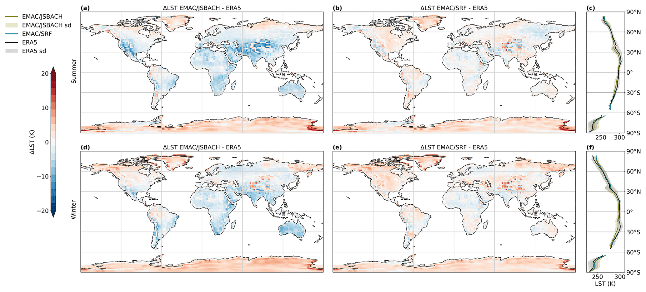
Figure 2 Difference in land surface temperature (LST) between EMAC/JSBACH and ERA5-Land during Northern Hemispheric (NH) summer (a) and NH winter (d) months, with data averaged over the years 1971 to 2010. Analogously, the difference between EMAC/SRF and ERA5-Land LST during summer (b) and winter (e) months is displayed. Positive values represent an overestimation of the simulated LST, while negative values indicate an underestimation. Additionally, the zonal average of all three datasets for both summer (c) and winter (f) months is shown. Here, LST from EMAC/JSBACH is depicted in green, LST from EMAC/SRF is shown in blue and LST from the ERA5-Land dataset is represented in black. The shaded area within the zonal mean plot illustrates the standard deviations along longitudes.

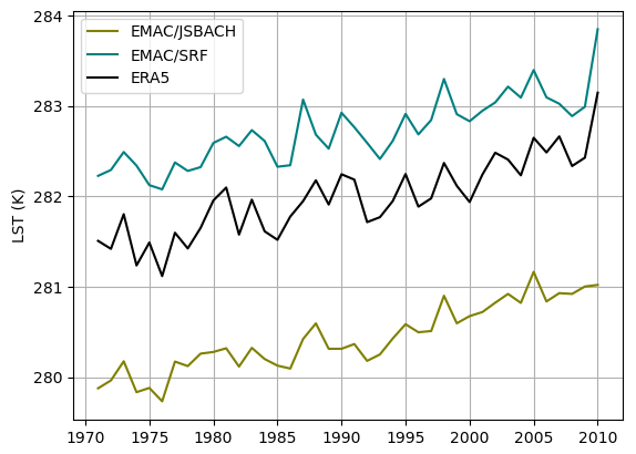
Figure 3 Globally averaged LST time series (in K) of EMAC/JSBACH (green), EMAC/SRF (blue) and ERA5 (black).

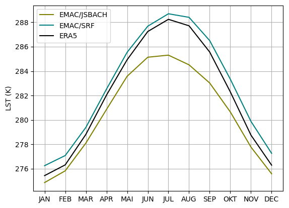
Figure 4 Globally averaged seasonal LST (in K) of EMAC/JSBACH (green), EMAC/SRF (blue) and ERA5 (black) for the years 1971 to 2010.

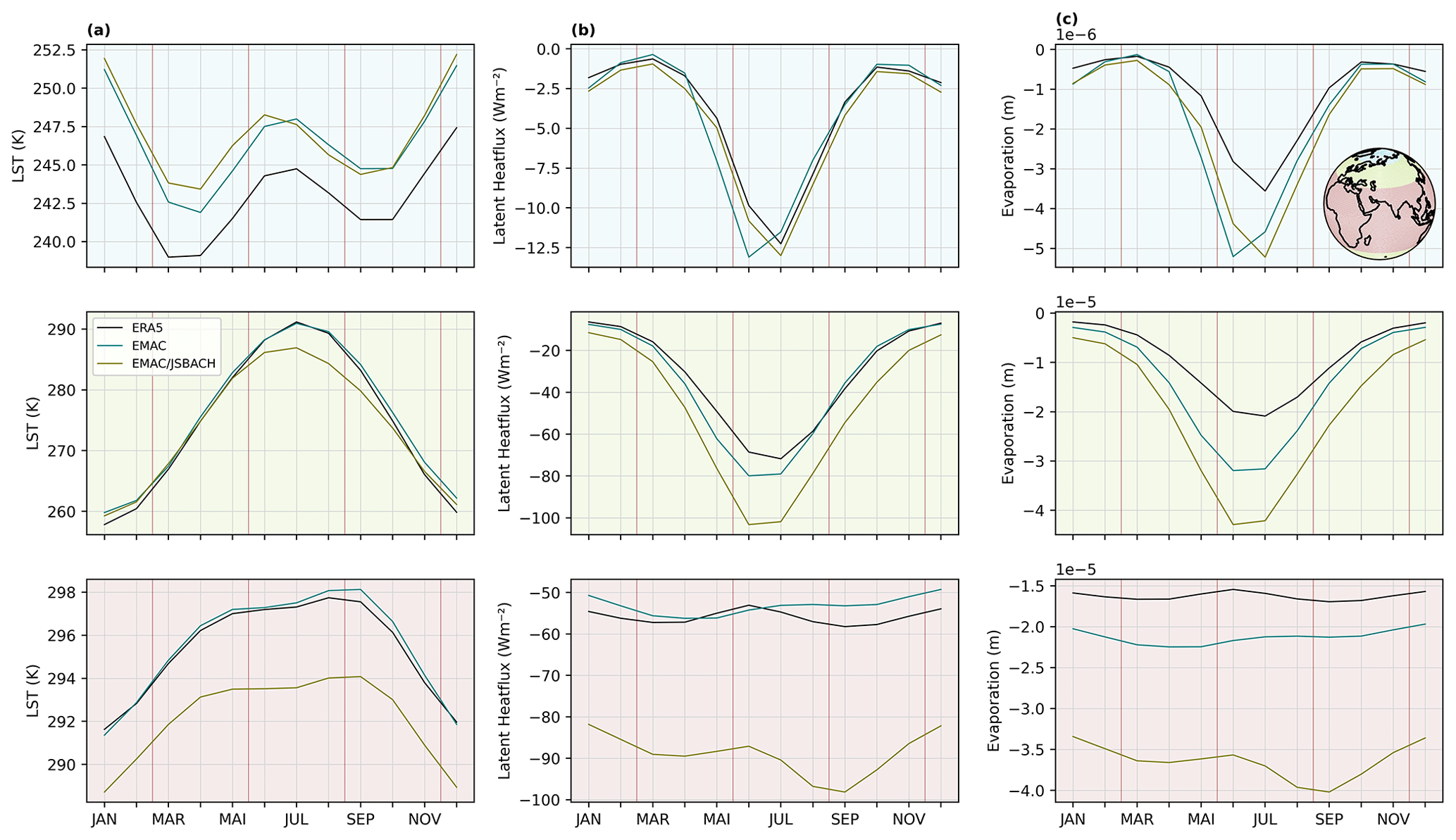
Figure 5 Averaged seasonal LST (in K), surface latent heat flux (in W m⁻²) and evaporation (without transpiration) (in m) of EMAC/JSBACH (green), EMAC/SRF (blue) and ERA5 (black) for the years 1971 to 2010. The upper panels indicate values averaged over the polar climate zone (latitudes > 66.5°), the mid panels values averaged over the temperate climate zone (latitudes between 40° and 66.5°) and the bottom panels values averaged over the tropical and subtropical climate zones (latitudes < 40°).

4.2 Terrestrial water storage (TWS)

The variation in soil depth of the reanalysis data and the model datasets complicates direct comparisons of the soil water content per layer. To overcome this problem, TWS is chosen as the evaluation variable. TWS is defined as the vertically integrated water content on land and the subsurface, including groundwater, rivers, lake water, soil moisture (also in the root zone), snow and ice (including permafrost), wet biomass, and water stored in vegetation (Girotto and Rodell, 2019). It depends on the amount of precipitation and the air temperature as well as on the soil type and infiltration, vegetation cover, surface and soil temperature, and runoff (Schneck et al., 2022).

For this assessment, however, we exclude water that drains from the land surface into rivers, streams or other waterbodies in order to focus only on the part of the water that is stored in the soil and vegetation. The TWS therefore includes all the water stored in a grid box; this total amount of water is comparable between the models and reanalysis.

In EMAC/JSBACH, the TWS is the sum of water content and runoff, calculated separately. The water content is calculated as the sum of all water reservoirs above and below ground, down to the bedrock. Everything below the bedrock, like deep groundwater and aquifers, is not represented in JSBACH and thus not taken into account (Reick et al., 2021). In EMAC/JSBACH, the soil water column is segmented into five layers, with a maximum depth of 9.834 m. The above-groundwater includes the wet skin reservoir (water on the canopy and surface) and snow on canopy and surface, both depending on and exchanging moisture between surface and atmosphere via precipitation, evaporation, sublimation, melting and windblow. TWS does not include any fluxes (such as evaporation). Water infiltrating the ground either percolates by gravitational movement (ending up as drainage if it reaches bedrock) or diffuses. Depending on its phase, it is defined as one of the EMAC/JSBACH below-groundwater reservoirs: soil moisture or soil ice. At the surface, the moisture exchange with the atmosphere occurs through evapotranspiration, dew formation or evaporation of bare soil, controlled by the specific humidity and temperature of the surrounding air. Furthermore, these processes strongly depend on vegetation coverage and, with that, plant productivity, which is also assessed via the gross primary productivity (GPP) (Sect. 4.8). TWS is compared to the ERA5-Land TWS, derived as the sum of the integrated volumetric soil water content, skin reservoir content and snow depth in metres water equivalent. The ERA5 soil water column is distributed over four layers, with a maximum depth of 2.89 m. Here, too, is the ERA5 dataset interpolated into the EMAC grid. Since TWS is not calculated for glaciers within EMAC/JSBACH, glaciated polar areas are excluded from this analysis.

In Fig. 6, the difference in TWS between EMAC/JSBACH and EMAC/SRF to ERA5 is shown. The annual global average of EMAC/JSBACH TWS weighted by latitudes is 0.029 m larger than the global mean of the ERA5. The maximum overestimation of TWS is found in western Russia (up to 3.0 m). EMAC/JSBACH overestimates TWS almost everywhere, independent of the season, except for high, elevated regions such as the Tibetan Plateau and Tien Shen, central and eastern Siberia, India (Deccan Plateau), the Ethiopian highlands, and Patagonia. Additionally, TWS is underestimated in the Amazon Basin.

The zonal mean of the EMAC/JSBACH TWS, as shown in Fig. 6 (right panels), does not exactly reproduce the zonal mean of the TWS from ERA5, but its absolute values are in better agreement with the ERA5 data than the EMAC/SRF results. This is also visible in Fig. 7, where the globally averaged TWS time series is illustrated. Since there are no snow cover data available from ERA5-Land for the year 1974, this year was excluded from the analysis. The TWS of the EMAC/SRF simulation (Fig. 6) is lower everywhere compared to the ERA5 dataset, except for deserts, where the TWS is low anyway. This leads to an annual global average of the EMAC/SRF TWS of 0.404 ± 0.202 m, which is different by −0.69 m than the one derived from reanalysis data (see Table 6). In EMAC/JSBACH, the global average of TWS is 1.123 ± 0.701 m, which is, with a difference of 0.029 m, significantly closer to ERA5 (1.094 ± 0.552 m).

The soil hydrology module that comes with EMAC/JSBACH offers the possibility of improving the representation of the soil water. The soil moisture in EMAC/SRF was simulated based on a simple bucket model. Following Seneviratne et al. (2010), this is now replaced by a more complex five-layer diffusive hydrological transport model that includes water storage and infiltration in five soil layers, preventing soil from drying too rapidly. While EMAC/SRF tends to strongly underestimate soil moisture levels everywhere, the integration of JSBACH results in larger and more spatially diverse soil moisture content. However, de Vrese et al. (2023) found that in the JSBACH version used here, infiltration only takes place if the temperature of the first soil layer is at or above the melting point. In combination with the five-layer snow scheme presented by Ekici et al. (2014), this becomes problematic. During spring snowmelt, soil temperatures are below the 0 °C of the overlying snow cover, causing all the meltwater to run off at the surface, while, in reality, a considerable amount should percolate into the soil (de Vrese et al., 2023). This contributes to the strong underestimation of TWS in permafrost regions, e.g. Siberia. Despite this, the global average time series analyses show that EMAC/JSBACH TWS aligns much more closely with the TWS from the ERA5 reanalysis compared to the EMAC/SRF results (Fig. 7).

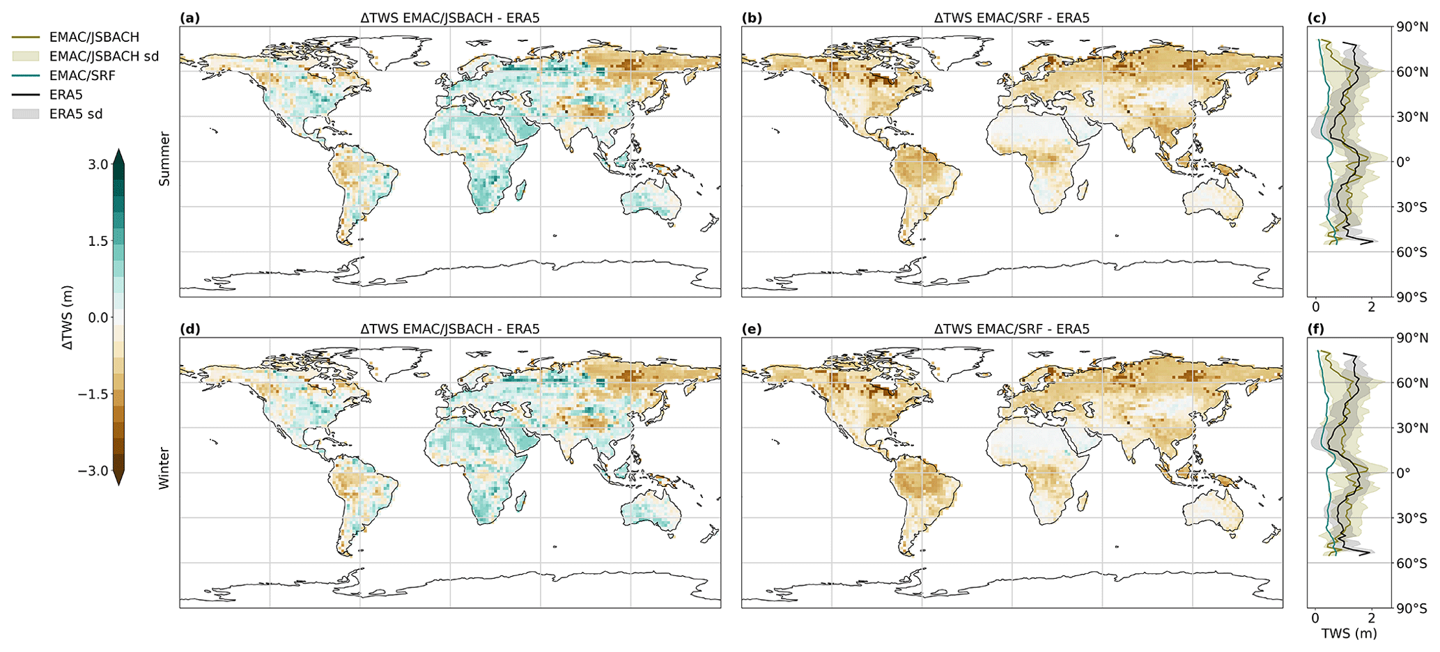
Figure 6 Difference in terrestrial water storage (TWS) between EMAC/JSBACH and ERA5-Land during NH summer (a) and NH winter (d) months, with data averaged over the years 1971 to 2010. Analogously, the difference between EMAC/SRF and ERA5-Land TWS during summer (b) and winter (e) months is displayed. Positive values represent an overestimation of the simulated TWS, while negative values indicate an underestimation. Additionally, the zonal average of all three datasets for both summer (c) and winter (f) months is shown. Here, TWS from EMAC/JSBACH is depicted in green, TWS from EMAC/SRF is shown in blue and TWS from the ERA5-Land dataset is represented in black. The shaded areas within the zonal mean plots illustrate the standard deviations of the datasets. Glaciated polar regions are excluded.

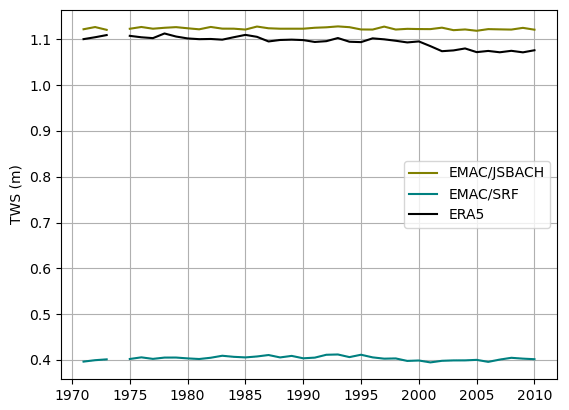
Figure 7 Globally averaged TWS time series (in m w.e.) of EMAC/JSBACH (green), EMAC/SRF (blue) and ERA5 (black).

4.3 Surface albedo (α)

Another key factor in Earth system modelling is the surface albedo as it is a fundamental input for the radiation scheme and strongly influences the energy budget of the planet. Generally defined as the reflected fraction of incoming solar radiation, it depends on the type of land cover and the extent and thickness of the snow cover or ice sheet. Especially over the continental area of the Northern Hemisphere and the sea ice cover in the Southern Hemisphere, the surface albedo can exert a strong feedback effect (Hall, 2004). Since the surface coverage of snow and ice can vary on small scales and is strongly coupled to atmospheric and oceanic dynamics, the computation of the surface albedo is still a challenging factor for GCMs (Bony et al., 2006). In EMAC/JSBACH, the surface albedo on glaciers is calculated for grid boxes either with ice sheets or without them, where these boxes are either completely or not at all covered with ice. For ice sheets, the albedo is calculated according to ECHAM5 (Roeckner et al., 2003). Every other surface is treated with a new albedo scheme based on the current state of snow cover, LAI, vegetation distribution and the spectral composition of solar downward radiation for each grid box, as described by Reick et al. (2021).

The surface albedo is compared to the ERA5-Land albedo variable. The ERA5-Land albedo is based on a 5-year MODIS climatology. These satellite observations are a combined Terra and Aqua retrieval (Schaaf and Wang, 2015). From the 16 d level-3 data of a 0.05° climate modelling grid (approx. 5.6 km at the Equator), monthly averages are calculated and interpolated into the EMAC T63 grid. The surface albedo of EMAC/JSBACH is, in general, in good agreement with the ERA5 surface albedo (Fig. 8). During summer, EMAC/JSBACH shows a slight overestimation over Europe and Asia between 45 and 75° N and parts of Canada. Between 25° S and 15° N, an underestimation is visible. During the northern winter months, North America and Canada show underestimated surface albedo along with Scandinavia, eastern Europe, northern Russia and elevated regions in Asia. The average annual global difference between EMAC/JSBACH and ERA5 is −0.015. The same geographical patterns are visible for the EMAC/SRF compared to ERA5 surface albedo comparison with average annual global difference of −0.012. The zonal mean shows a slight overestimation of surface albedo for both simulations in the southern subtropics during summer and winter. During winter, there is a minimum of the surface albedo at about 45° N, which is not seen in the reference data (Fig. 8, right panels).

The land surface albedo remains almost unchanged in the new model version. This is presumably due to the fact that in EMAC/SRF the background albedo is temporally constant except for changes in ice and snow cover (Nützel et al., 2023). In EMAC/JSBACH, a simplified ground albedo scheme was used to obtain a comparable result. However, there is a slight improvement compared to the reference data for EMAC/JSBACH, which is particularly noticeable during the summer in eastern Siberia, where the model overestimation is reduced. In this region, the LST and LAI derived from EMAC/JSBACH align more closely to the reference data than EMAC/SRF alone. This suggests that the slightly warmer surface and less vegetation in this region may contribute to the improved surface albedo representation.

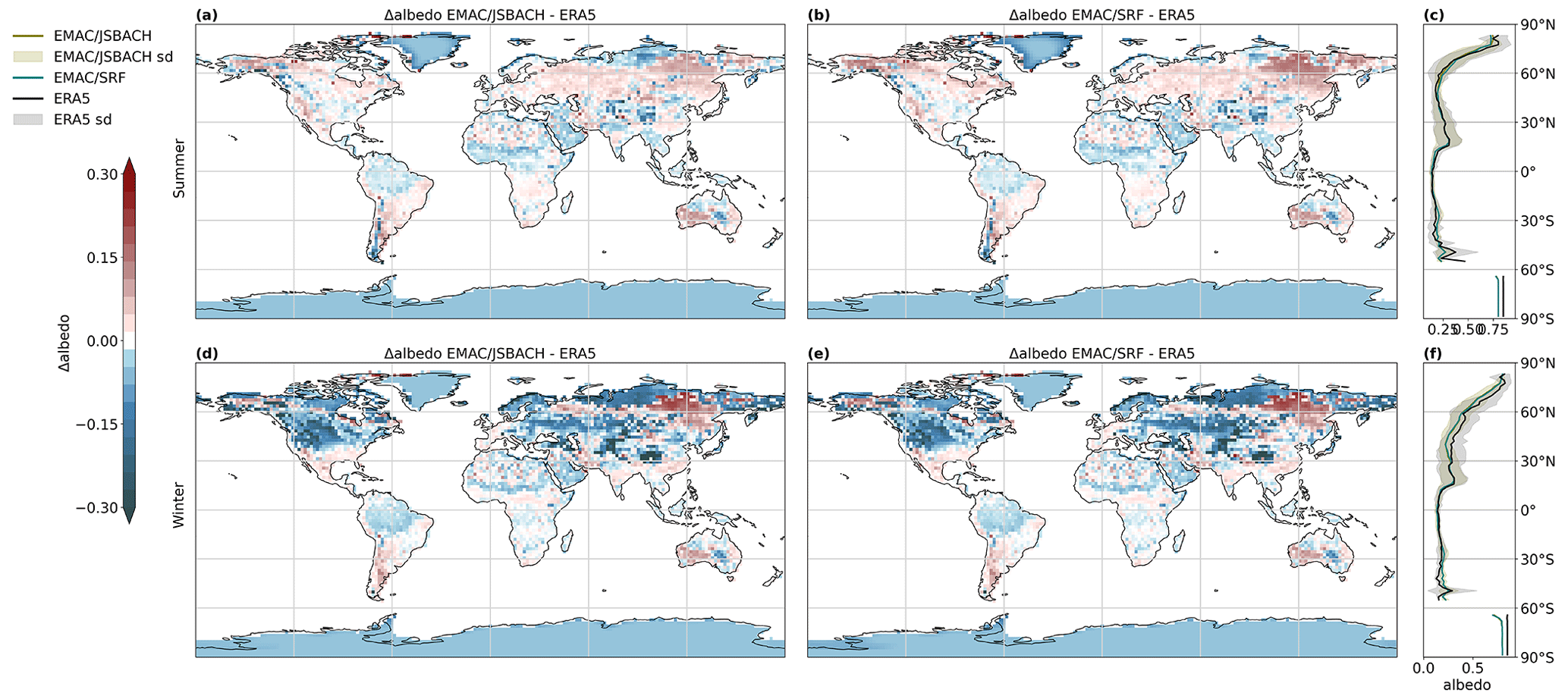
Figure 8 Difference in surface albedo (α) between EMAC/JSBACH and ERA5-Land during Northern Hemispheric (NH) summer (a) and NH winter (d) months, with data averaged over the years 1971 to 2010. Analogously, the difference between EMAC/SRF and ERA5-Land α during summer (b) and winter (e) months is displayed. Positive values represent an overestimation of the simulated α, while negative values indicate an underestimation. Additionally, the zonal average of all three datasets for both summer (c) and winter (f) months is shown. Here, α from EMAC/JSBACH is depicted in green, α from EMAC/SRF is shown in blue and α from the ERA5-Land dataset is represented in black. The shaded area within the zonal mean plot illustrates the standard deviations along longitudes.

4.4 Top-of-atmosphere radiation balance (Rad_TOA)

The top-of-atmosphere (TOA) net radiation can be defined as the difference between the incoming solar radiation; outgoing solar radiation backscattered and reflected by clouds, aerosols, air and the land surface; and the terrestrial radiation emitted by the surface, atmosphere and clouds. In total and in equilibrium, the multi-year global mean sum should be zero. However, as climate change continues and the amount of greenhouse gases in the atmosphere increases, this effect exceeds zero; i.e. more radiation is trapped in the atmosphere than is emitted, leading to global warming. In climate modelling, the amounts of radiative energy absorbed and emitted in and by the atmosphere are key factors in the Earth's energy balance. The concentration of water vapour in the atmosphere and the surface albedo are important factors (Loeb et al., 2009). It is important to reproduce these factors correctly and to detect possible biases. The radiation fluxes are calculated by the MESSy submodel RAD, which is a new implementation of the ECHAM5 radiation scheme (Dietmüller et al., 2016). Rad_TOA is compared to the ERA5 monthly averaged reanalysis data of TOA solar and terrestrial radiation interpolated into the EMAC T63 grid (Hersbach et al., 2023).

The average temporal and spacial correlation between EMAC/JSBACH and ERA5 Rad_TOA is 0.907 (Table 6). The largest differences and overestimation of EMAC/JSBACH Rad_TOA in comparison to ERA5 during the summer months occur over north and west Africa and the Middle East (Fig. 9). The best agreement is found during summer over western Russia. The largest underestimations are found over central Africa and northern South America. During winter, the largest overestimation occurs over the Himalayas and the largest underestimation over the northern and southern Andes, central Africa, and Indonesia. During this time period, the best agreement is found over the polar and sub-polar regions. The average annual global difference between EMAC/JSBACH and ERA5 is 3.56 W m⁻². The zonal mean of the simulation is well in line with the zonal mean of the reanalysis data, and the overestimation of the simulation only occurs at 30° N and between 0 and 30° S. Comparing EMAC/SRF and ERA5, a similar geographical distribution is discernable and, especially in winter, there is almost no difference to the EMAC/JSBACH simulation. However, almost everywhere at high latitudes, the TOA radiative flux is lower during summer. The same applies for the zonal average. The average annual global difference between EMAC/SRF and ERA5 is 3.045 W m⁻², and the overall correlation is 0.909.

The TOA radiation derived from EMAC/JSBACH shows noticeable regional variations when compared to reanalysis data, yet its overall balance remains comparable to the one derived from EMAC/SRF. Moreover, these regional differences in Rad_TOA closely align with those observed for EMAC/SRF and do not significantly change when EMAC is in operation without JSBACH. Rad_TOA shows a strong anti-correlation with the surface albedo ($\mathit{\rho }=-\mathrm{0.86}$), which determines the amount of absorbed radiation on the surface (Table A2 in the Appendix). Since there are no significant differences between the EMAC/SRF and EMAC/JSBACH surface albedo, no significant differences in Rad_TOA are expected.

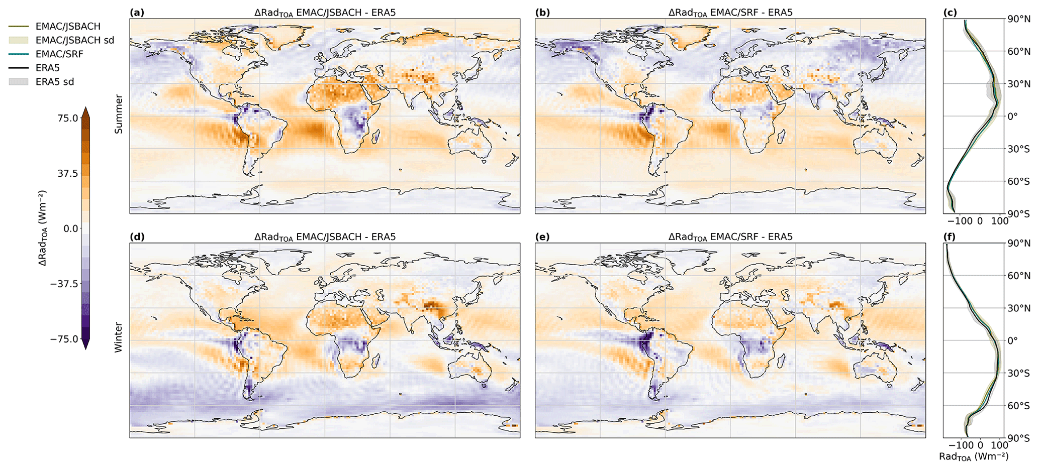
Figure 9 Difference in top-of-atmosphere radiation (Rad_TOA) between EMAC/JSBACH and ERA5 during Northern Hemispheric (NH) summer (a) and NH winter (d) months, with data averaged over the years 1971 to 2010. Analogously, the difference between EMAC/SRF and ERA5 Rad_TOA during summer (b) and winter (e) months is displayed. Positive values represent an overestimation of the simulated Rad_TOA, while negative values indicate an underestimation. Additionally, the zonal average of all three datasets for both summer (c) and winter (f) months is shown. Here, Rad_TOA from EMAC/JSBACH is depicted in green, Rad_TOA from EMAC/SRF is shown in blue and Rad_TOA from the ERA5 dataset is represented in black. The shaded area within the zonal mean plot illustrates the standard deviations along longitudes.

4.5 Precipitation (precip)

Since precipitation is one of the most important and challenging climate variables to reproduce for coupled global climate models (Dai, 2006), we are interested in analysing the general performance of the coupled EMAC/JSBACH and EMAC/SRF simulations to reproduce regional and temporal variations as well as the amount and intensity of precipitation. Problems of the simulation of precipitation can be an indication of issues of the processes that drive precipitation, such as large- and small-scale atmospheric dynamics, cloud micro-physics, and aerosol formation (Dai, 2006). Precipitation is calculated by the submodels CLOUD and CONVECT and is one of the standard input parameters for EMAC/JSBACH, forcing many processes in the land system. The simulated precipitation is compared to the Global Precipitation Climatology Project (GPCP) dataset of monthly precipitation spanning 1979 to 2021 (Adler et al., 2003). The observational precipitation data are available at a grid resolution of 2.5° ×2.5°, which is approximately 280 km at the Equator, and is regridded to the EMAC Gaussian T63 grid (1.8° × 1.8°, approximately 210 km at the Equator) using bi-linear interpolation. The dataset provides an error estimate, which is defined for every data point present in the dataset. This assessment considers solely the stochastic error and relies on both the mean rainfall rate and the quantity of samples utilized for its computation (Huffman, 1997). The differences between global precipitation distributions are shown in Fig. 10. The subtropical and tropical equatorial zones over land appear drier in the EMAC/JSBACH simulation in comparison to the GPCP data. This shifts from the Northern Hemisphere during summer to the Southern Hemisphere during winter. Over the oceans, regions of heavy precipitation are intensified in the simulation. The average annual global difference between EMAC/JSBACH and ERA5 is 0.042 mm d⁻¹ (2.738 to 2.696 mm d⁻¹; see Table 6). For the GPCP dataset, the error is shown as a grey-shaded area within the zonal mean plot. Zonally averaged, EMAC/JSBACH summer precipitation is within the GPCP precipitation error for the tropics and mid-latitudes, with EMAC/JSBACH underestimating precipitation at high latitudes. In the tropical region of the Northern Hemisphere, EMAC/JSBACH also slightly overestimates precipitation during winter. The northern Inter-Tropical Convergence Zone (ITCZ) is reproduced in agreement with the observations by the EMAC/SRF and EMAC/JSBACH simulations. The comparison between EMAC/SRF and GPCP shows that the simulated precipitation amounts are higher than the observed ones, with an average annual global deviation of 0.329 mm d⁻¹. Similar to EMAC/JSBACH, this simulation shows lower precipitation over Indonesia compared to the GPCP data. Particularly noticeable is the tendency to overestimate precipitation over land, especially in the Himalayas in summer and in the Andes in winter. This is also evident in the zonal mean, although EMAC/SRF remains within the margin of error in the observations in summer. The only exception is the tropical regions of the Northern Hemisphere, where there is more precipitation in winter and less around 60° S.

Overall, EMAC/JSBACH is capable of reproducing global precipitation to a similar extent as EMAC/SRF. It exhibits a distinct wet bias zone, extending from 20° S to the Equator during winter and from 20° N to the Equator during summer (Fig. 11). This wet bias band is adjacent to a dry bias region, ranging from 0–10° N during NH winter and from 0–25° S during NH summer. The same is found for the precipitation derived from EMAC/SRF (Fig. 11) and leads to the assumption that there is no major change in the large-scale atmospheric dynamics of the new coupled model. The wet bias will be corrected by further “tuning” microphysical parameters in upcoming model versions. The dry biases over the Arctic and Antarctic regions throughout the year may be attributed to relatively low sea surface temperatures. This relationship has previously been documented by Pozzer et al. (2011a).

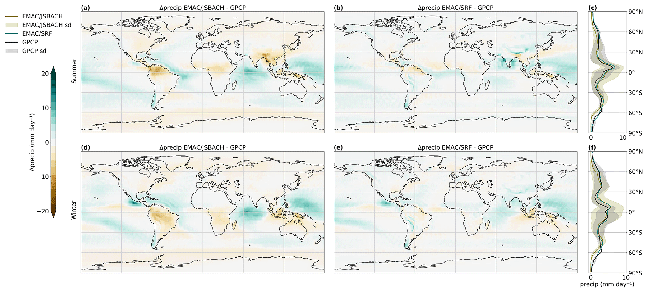
Figure 10 Difference in precipitation between EMAC/JSBACH and GPCP during Northern Hemispheric (NH) summer (a) and NH winter (d) months, with data averaged over the years 1980 to 2010. Analogously, the difference between EMAC/SRF and GPCP precipitation during summer (b) and winter (e) months is displayed. Positive values represent an overestimation of the simulated precipitation, while negative values indicate an underestimation. Additionally, the zonal average of all three datasets for both summer (c) and winter (f) months is shown. Here, precipitation from EMAC/JSBACH is depicted in green, precipitation from EMAC/SRF is shown in blue and precipitation from the GPCP dataset is represented in black. The shaded area within the zonal mean plot in black illustrates the GPCP dataset error and in green the standard deviation of the EMAC/JSBACH precipitation.

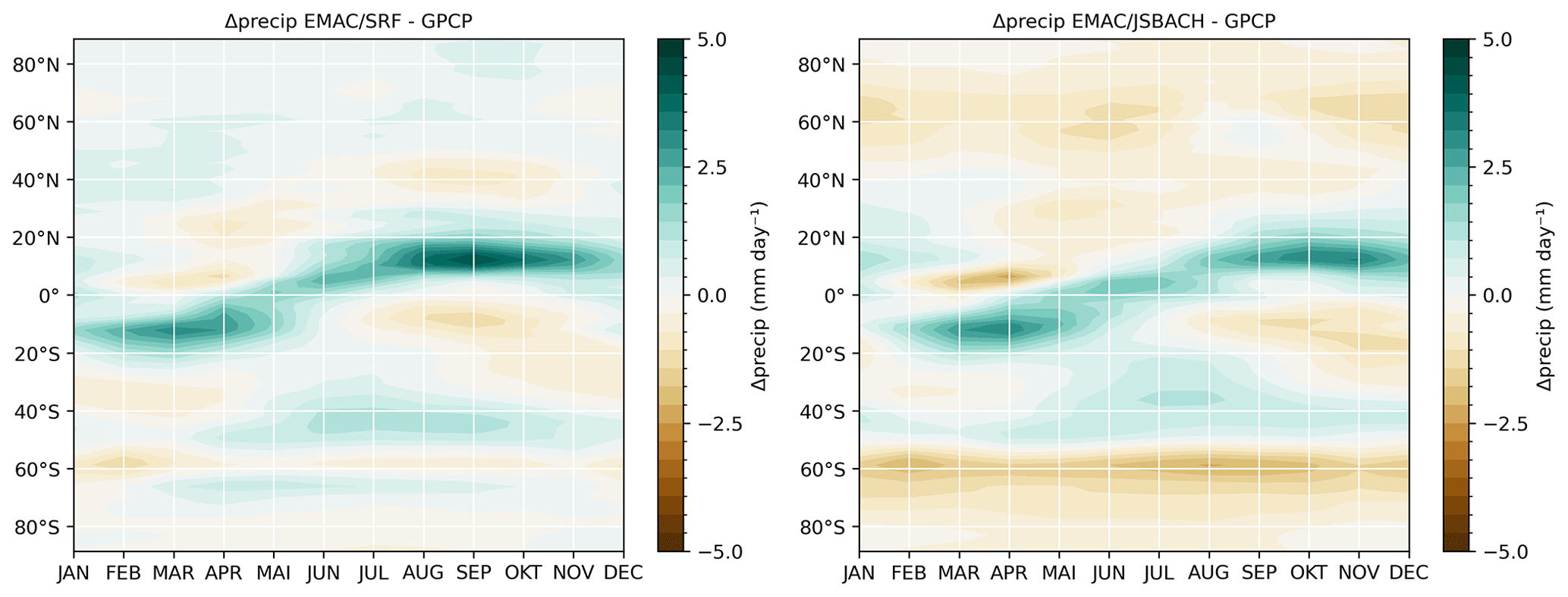
Figure 11 Zonally averaged monthly difference in EMAC/JSBACH (a) and EMAC/SRF (b) compared to GPCP precipitation in millimetres per day, averaged over the years 1980 to 2010.

4.6 Leaf area index (LAI)

The leaf area index is defined by Watson (1947) as the total one-sided area of leaf tissue per unit of ground surface area. It is an important quantity for estimating the gas exchange between vegetation and the atmosphere in particular (e.g. photosynthetic production or transpiration) and represents the canopy–atmosphere interface (Bréda, 2003). It has a strong spatial and temporal variability, which makes it difficult to properly measure and simulate it. The default scheme to calculate the LAI in JSBACHv4 is an implementation of the Logistic Growth Phenology (LoGro-P) model, which is described in detail by Böttcher et al. (2016) and Reick et al. (2021). Within LoGro-P, the LAI is calculated depending on the phenology type of the plant functional types (PFTs), which are either evergreen, summergreen, raingreen, grasses, or tropical or extratropical crops. Due to the prescribed geographical PFT distribution, there is no seasonal or inter-annual variability in plant functional types, limiting LAI variability. The phenology types are linked to certain phenology phases. For the summergreen type, these are, in turn, associated with seasons. Spring corresponds to the growth phase, summer to the vegetative phase, and winter and autumn to the resting phase (Schneck et al., 2022). Raingreen, grass, and tropical crop phenology types are only linked to a growth phase determined by environmental conditions like soil moisture, temperature and NPP, growing whenever those conditions are beneficial (Schneck et al., 2022). Tropical or extratropical crops are not linked to a vegetative phase. The LAI changes primarily due to temperature, soil moisture and NPP, and the maximum possible value is limited for each phenology type individually (Schneck et al., 2022). The LAI is compared to the 8-Day global MODIS/Terra Leaf Area Index dataset, regridded to 0.5° resolution (Kern, 2023; Myneni, 2021). Monthly averages are calculated and interpolated into the EMAC T63L31 grid.

The LAI difference between the EMAC/JSBACH and MODIS observations is shown in Fig. 12. The annual global average LAI within EMAC/JSBACH is −0.212 m² m⁻² (1.187 to 1.399 m² m⁻²; see Table 6) lower than the one estimated using MODIS satellite data. In particular, the LAI of tropical rainforests is underestimated throughout the year in the simulation, as are deciduous forests and boreal forests over eastern Siberia in summer. Otherwise, vegetation LAI tends to be overestimated, with peaks in India, south Africa and northern Canada throughout the year and in northern Europe during the winter. The zonal average (Fig. 12, right panels) shows that EMAC/JSBACH follows the MODIS LAI trend but with lower peak values at the Equator. EMAC/SRF overestimates LAI in comparison to the MODIS dataset almost everywhere, and the annual global average LAI is 0.768 m² m⁻² larger than the satellite-instrument-based estimate. Maximum overestimations are found for the Amazon rain forest and Canadian boreal forest throughout the year. The same is found for the zonal average, of which the EMAC/SRF LAI peaks at the Equator at 7.5 m² m⁻².

Discrepancies between EMAC/SRF and EMAC/JSBACH LAI are expected, due to EMAC/SRF's reliance on a LAI climatology, whereas in EMAC/JSBACH LAI is a prognostic variable. In JSBACH, the calculation of LAI for raingreen and crop phenology strongly depends on water availability. Tropical raingreen phenology is found in regions such as the Amazon, Indonesia and central Africa. These regions exhibit low TWS and coincide with regions of underestimated LAI. Over India, the phenology only consists of tropical broadleaf deciduous forests and both C₃ and C₄ crops. Given that the water deficit in India is not as pronounced as in other areas, the overestimation of LAI in India may be partly attributed to sufficient moisture content in the soil. In addition, GPP is enhanced in this area. This results in a feedback loop as more vegetation leads to greater LAI, which in turn increases GPP and NPP, thus stimulating plant growth. The overestimation of LAI of extratropical evergreen and summergreen phenology, such as in northern Canada and Europe, is not determined by water availability since those LAI calculations are only based on parameterisations governing phenology and a set of parameters defining growth rate and the length of the growth season. Schneck et al. (2022) stated that an unlucky choice of those parameters can have a major effect on LAI estimation. However, Lin et al. (2023) found that the MODIS version 6.1 leaf area index product tends to underestimate LAI particularly in northern latitudes, which may contribute to the bias found over northern Canada and Europe.

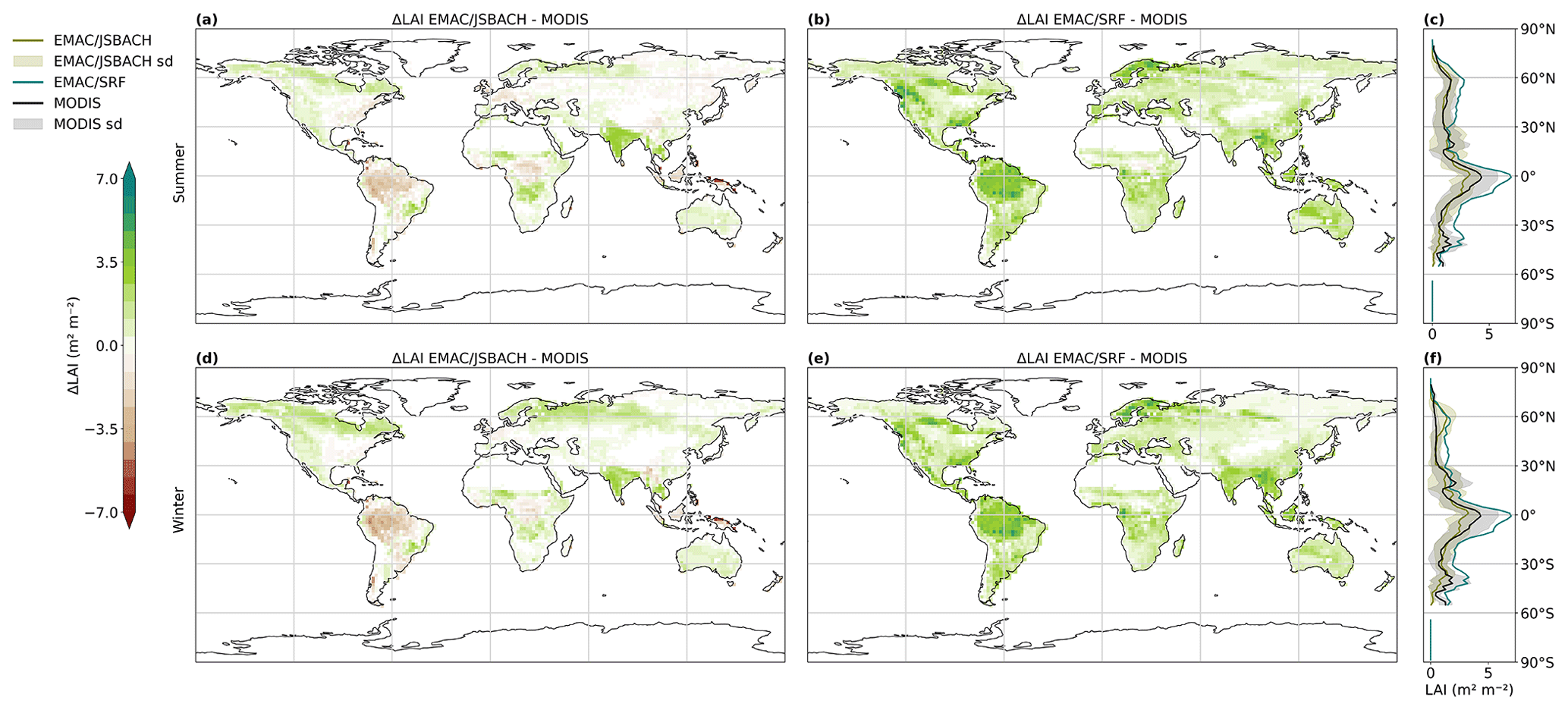
Figure 12 Difference in LAI between EMAC/JSBACH and MODIS during Northern Hemispheric (NH) summer (a) and NH winter (d) months, with data averaged over the years 2000 to 2010. Analogously, the difference between EMAC/SRF and MODIS LAI during summer (b) and winter (e) months is displayed. Positive values represent an overestimation of the simulated LAI, while negative values indicate an underestimation. Additionally, the zonal average of all three datasets for both summer (c) and winter (f) months is shown. Here, LAI from EMAC/JSBACH is depicted in green, LAI from EMAC/SRF is shown in blue and LAI from the MODIS dataset is represented in black. The shaded area within the zonal mean plot illustrates the standard deviations along longitudes.

4.7 Fraction of absorbed photosynthetic active radiation (FAPAR)

Together with the LAI, the fraction of absorbed photosynthetic active radiation is required to estimate the ecosystem productivity. It is a state variable that describes the amount of incoming solar radiation which is absorbed by leaves and available for photosynthesis. The absorption happens in the photosynthetic active radiation (PAR) band of 400–700 nm (Sellers, 1985) and depends on the solar zenith angle, the canopy thickness, the types of leaves, their optical properties, the orientation and the soil underneath (Reick et al., 2021).

In EMAC/JSBACH FAPAR is calculated in three canopy layers by the canopy radiation module, which is described by Loew et al. (2014) and Reick et al. (2021) in detail. After the calculation, FAPAR is handed over to the photosynthesis module and used to estimate the gross and net primary productivity and carbon fixation in the plants.

We compare our results to 8-Day Global MODIS/Terra Leaf Area Index dataset, regridded to global data at 0.5 resolution derived by the Integrated Climate Data Center (ICDC) (Kern, 2023; Myneni, 2021). Monthly averages are calculated and interpolated into the EMAC T63 grid.

The fraction of absorbed photosynthetic active radiation (FAPAR) is a newly introduced variable that was not available as EMAC output before the coupling to JSBACH. When compared to MODIS, the simulated FAPAR in EMAC/JSBACH is systematically underestimated across most regions, with the exception of India and northern Canada (Fig. 13). This underestimation is also evident in the zonal average. The annual global average FAPAR simulated by EMAC/JSBACH is 0.161 ± 0.137, whereas MODIS data indicate a higher average of 0.384 ± 0.196. Disney et al. (2016) conducted a comparison between the MODIS product and FAPAR and LAI measurements obtained from the ESA GlobAlbedo product. GlobAlbedo aligns with the 1D radiative transfer schemes used in EMAC/JSBACH and other large-scale ESMs. Their findings indicated overall good agreement in terms of timing between the datasets. Nevertheless, notable discrepancies in peak values were detected, with GlobAlbedo-derived values generally registering as lower compared to MODIS. They also state that the method used to determine FAPAR can result in variations of up to an order of magnitude difference. Loew et al. (2014) found a difference of up to 25 % when comparing models and satellite observations. These biases can be attributed, in part, to uncertainties in total cloud cover and snow cover that may affect satellite-based measurements. However, they may also result from the underlying definitions and algorithms used to determine the FAPAR product by satellite instruments (Loew et al., 2014). Within EMAC/JSBACH, the largest potential cause of uncertainty is the bias of the LAI, which, for example, most likely leads to the overestimation of FAPAR over India. Additionally, it cannot be ruled out that the representation of the surface albedo and the radiative transfer scheme might lead to the general underestimation of FAPAR, as was also documented in former studies (Loew et al., 2014; Disney et al., 2016). The differences in EMAC and observations in the radiative fluxes (mentioned above), especially the shortwave components, might also substantially contribute to the bias in FAPAR.

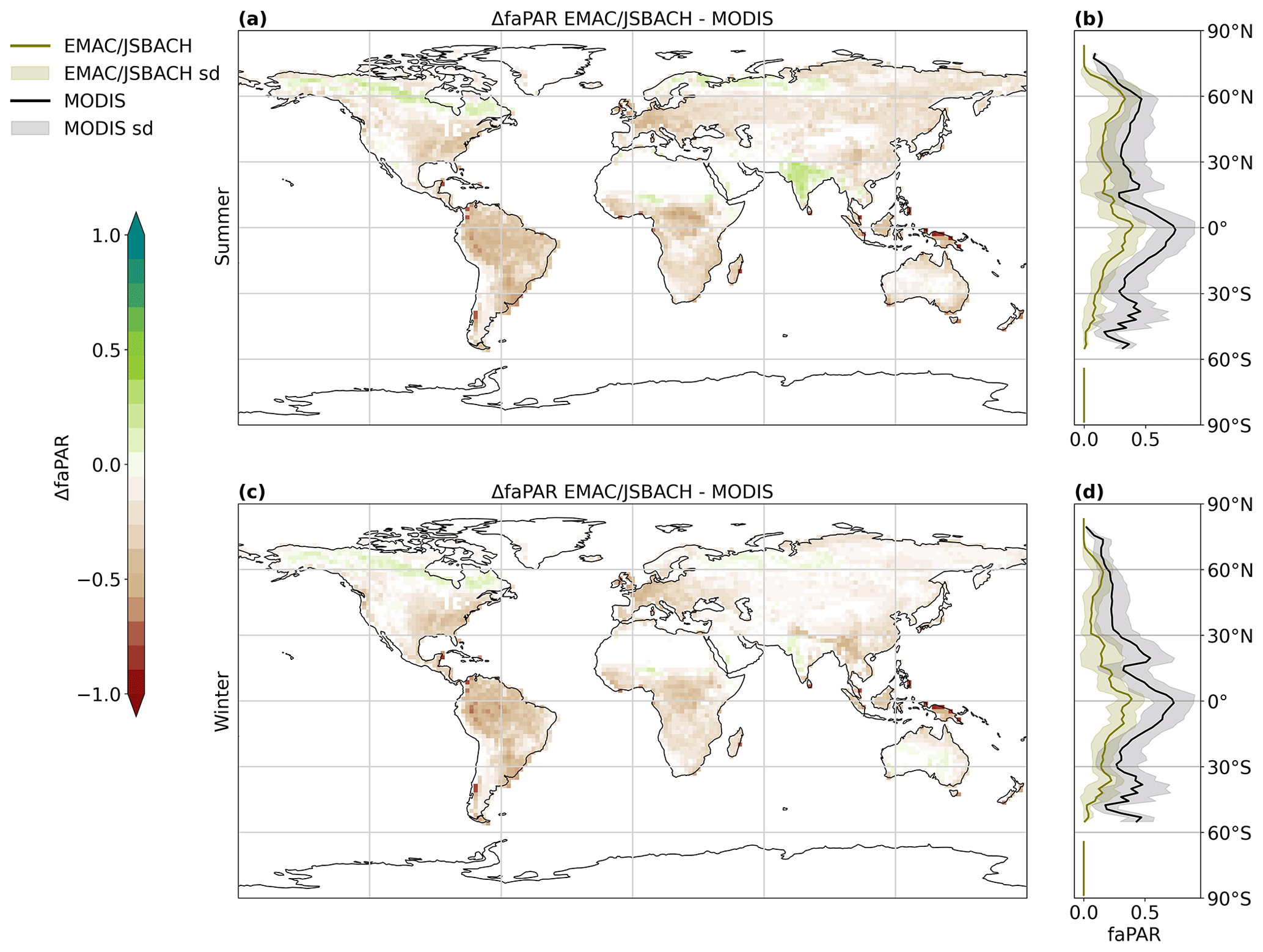
Figure 13 Difference in the fraction of absorbed photosynthetic active radiation (FAPAR) between EMAC/JSBACH and MODIS during Northern Hemispheric (NH) summer (a) and NH winter (c) months, with data averaged over the years 2000 to 2010. Positive values represent an overestimation of the simulated FAPAR, while negative values indicate an underestimation. Additionally, the zonal average of both datasets for both summer (b) and winter (d) months is shown. Here, FAPAR from EMAC/JSBACH is depicted in green and FAPAR from the MODIS dataset is represented in black. The shaded area within the zonal mean plot illustrates the standard deviations along longitudes.

4.8 Gross primary productivity (GPP)

Gross primary productivity is the total rate of organic carbon gained via photosynthesis. This includes autotrophic respiration, which can be divided into maintenance respiration (driving basic functionalities of the plant, like water and nutrient transport, defence mechanisms, or repairs) and growth respiration. GPP is a key parameter in estimating the net primary productivity (NPP), which describes the actual amount of carbon (sugars) stored in vegetation and is, therefore, an important quantity for the terrestrial carbon cycle. It is highly dependent on radiation, temperature, precipitation, LAI, TWS and water usage efficiency (the amount of water used by the plant to assimilate carbon). In EMAC/JSBACH, GPP is calculated via carbon assimilation (based on the plant water stress), FAPAR and LAI. The full and detailed description of the dynamics of vegetation carbon is provided by Reick et al. (2021).

GPP is compared to the MOD17A2H MODIS/Terra gross primary productivity 8-Day L4 Global 500m SIN Grid V006 regridded to global data at 0.5 resolution derived by ICDC (Kern, 2021; Running et al., 2015). Monthly averages are calculated and interpolated into the EMAC T63 grid.

Similar to FAPAR, gross primary productivity is a new diagnostic introduced in EMAC by JSBACH. GPP shows the largest differences to MODIS observations during NH summer over India, where GPP is strongly overestimated (Fig. 14). These are slightly lower during winter, when the GPP overestimation is larger over Australia and central South America. The largest underestimation is found during summer month over northeastern Siberia, the Amazon region and central Africa, while, during summer, the largest underestimation is found in the Amazon Basin and the Andes. The annual global average GPP of EMAC/JSBACH is 0.02 ± 0.017 kg carbon km⁻², while that of MODIS is 0.021 ± 0.013 kg carbon km⁻².

GPP underestimations are mostly found in areas where TWS and FAPAR are also underestimated. The correlation between TWS and GPP is ρ=0.79, indicating a monotonic relationship (Table A2 in the Appendix). The correlation between FAPAR and GPP is, as expected, high, with 0.94, since the GPP calculation is based on FAPAR. However, in this study, GPP demonstrates a notably better agreement with MODIS observations than FAPAR. The pronounced overestimation of GPP over India can be largely attributed to the concurrent overestimation of FAPAR in that region, which, in turn, can be traced back to the high LAI values that are prevalent there. In the global mean, FAPAR derived from EMAC/JSBACH and MODIS are in good agreement.

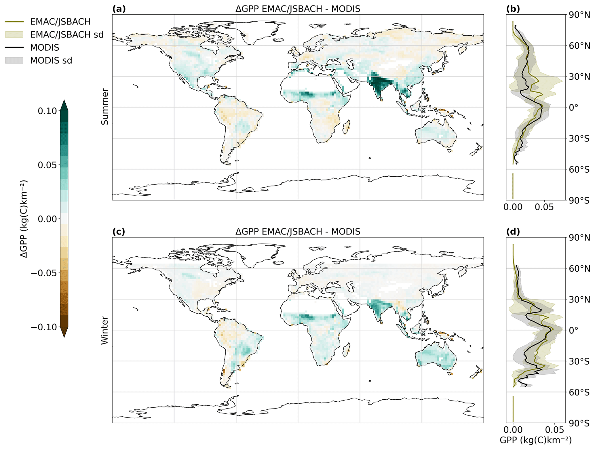
Figure 14 Difference in gross primary productivity (GPP) between EMAC/JSBACH and MODIS during Northern Hemispheric (NH) summer (a) and NH winter (c) months, with data averaged over the years 2000 to 2010. Positive values represent an overestimation of the simulated GPP, while negative values indicate an underestimation. Additionally, the zonal average of both datasets for both summer (b) and winter (d) months is shown. Here, GPP from EMAC/JSBACH is depicted in green and GPP from the MODIS dataset is represented in black. The shaded area within the zonal mean plot illustrates the standard deviations along longitudes.

5 Conclusions

We have implemented the land surface model JSBACH version 4 as a new submodel into EMAC following the MESSy coding standards. The new addition aims to replace of the former, simplified submodel SURFACE, in which many parameters have been prescribed based on pre-determined climatologies. JSBACH comprises numerous new features, including a comprehensive hydrology model and an improved soil scheme, enhancing the overall versatility of EMAC. It enables the possibility of performing new experiments that analyse not only the fundamental physical processes of the land surface within the Earth system on climatic timescales, but also the effects of atmospheric chemical components and associated feedback mechanisms on short timescales of hours and days. In this assessment, we demonstrate that the implementation, various modifications, and newly added features to EMAC have not degraded the overall model performance and stability. This is done based on a comparison of the new coupled model results to observational and reanalysis data and in comparison to results from a simulation conducted without JSBACH (i.e. based on climatologies). The newly coupled land–atmosphere model, however, required re-tuning to optimise the radiation budget via adjusted cloud parameters. The usage of JSBACH instead of SURFACE increases the runtime, on average, by 0.056 % $\pm \mathrm{4}\times {\mathrm{10}}^{-\mathrm{4}}$ % for simulations carried out on two computing nodes of the DKRZ (German Climate Computing Centre) supercomputer LEVANTE.

Results indicate that the LST derived from the newly coupled EMAC/JSBACH model is, on average globally, 1.546 K colder compared to the LST derived from ERA5 (using the old SURFACE submodel, the globally averaged LST was 0.816 K warmer). The change from SURFACE to JSBACH improves the representation of TWS by generally increasing soil moisture and groundwater storage. This improves the agreement of the absolute global average TWS with the ERA5-Land reanalysis data and reduces the NRMSE. Surface albedo and Rad_TOA balance show no significant changes after the implementation of JSBACH. While seasonal and regional precipitation patterns are preserved, the global mean precipitation is slightly reduced in EMAC/JSBACH. The average global LAI of the EMAC/JSBACH simulation agrees better with the average LAI of MODIS than the climatological standard LAI present in EMAC/SRF; nevertheless, the spacial and temporal correlation of 0.637 between simulated LAI and observed LAI is still not very high. FAPAR and GPP are among many other newly introduced variables that were not available in previous EMAC versions (a selection of the additional output variables is included in the Supplement). They are now provided as diagnostic parameters. FAPAR shows the largest deviation from the observations, which could partly be due to challenges in observing and quantifying FAPAR. Nevertheless, FAPAR as a fundamental parameter within the GPP calculations seems realistic, as the GPP and observational global average difference are only −0.001 kg carbon km⁻¹.

We plan to implement the remaining JSBACH4 features, such as the closed carbon cycle and dynamic vegetation. The latter can be achieved before these updates are available by linking JSBACH with the dynamic vegetation of the LPJ-GUESS module that is already coupled with EMAC (Forrest et al., 2020). The model will be further refined to increase its capabilities and accuracy. This ongoing model development is crucial to striving towards the more comprehensive and realistic numerical modelling of the intricate interactions between the atmosphere and land along with the associated feedback mechanisms. It marks a significant advancement for EMAC, bringing it one step closer to the realisation of a comprehensive Earth system model.

Appendix A

Table A1 EMAC/JSBACH land cover types (lct) and corresponding tile in the EMAC/JSBACH simulation.

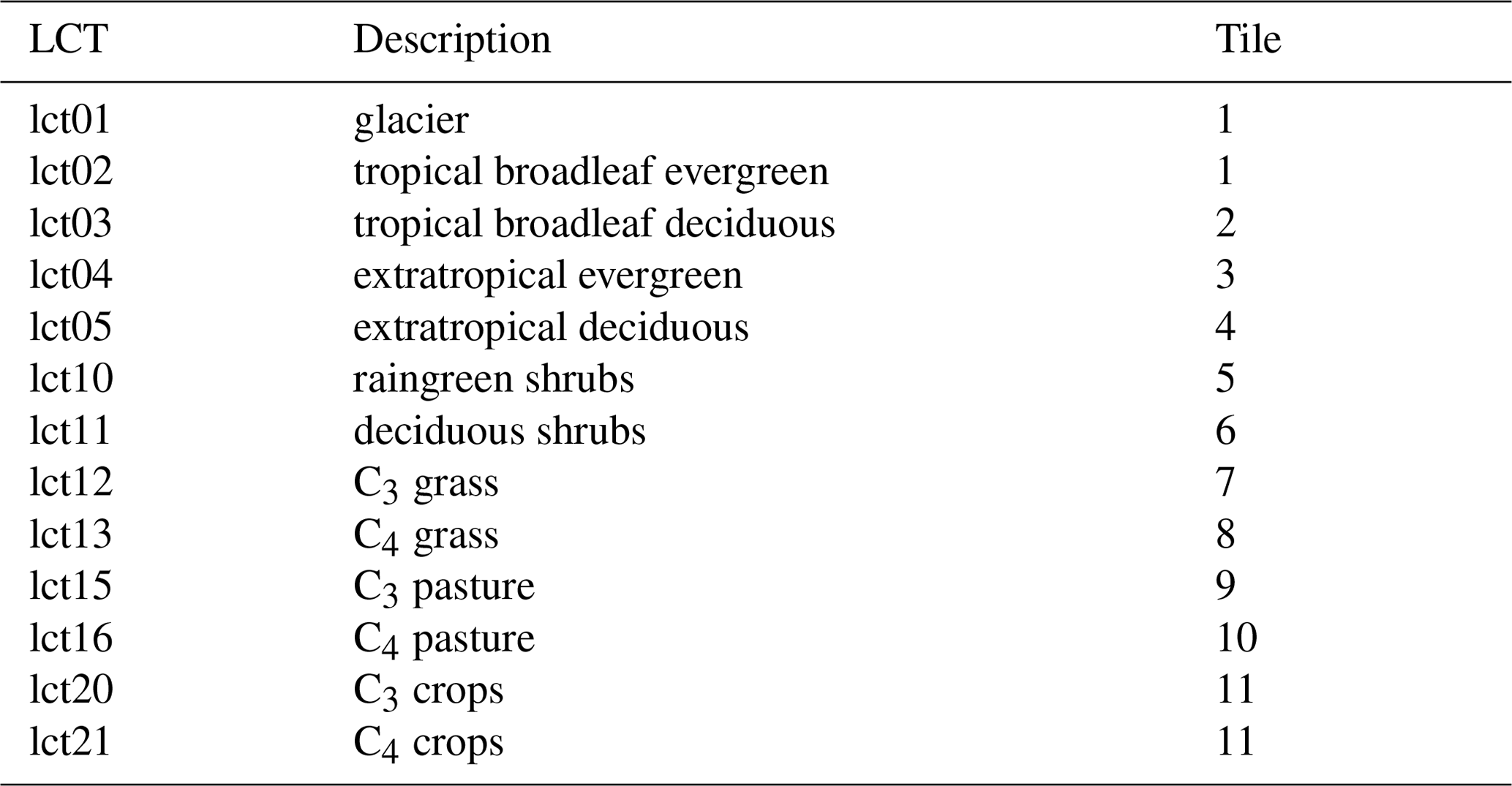
Table A2 Spearman rank correlation (ρ) of the assessed variables derived from monthly means of EMAC/JSBACH for the years 1971 to 2010. A positive Spearman rank correlation suggests a monotonously increasing relationship, while a negative correlation indicates a monotonously decreasing relationship. All correlations were tested for statistical significance at the p<0.05 level.

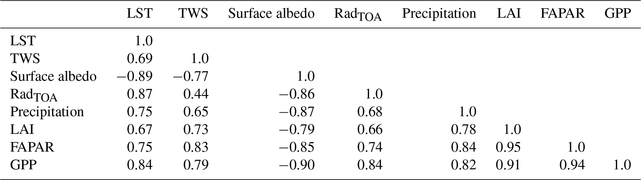
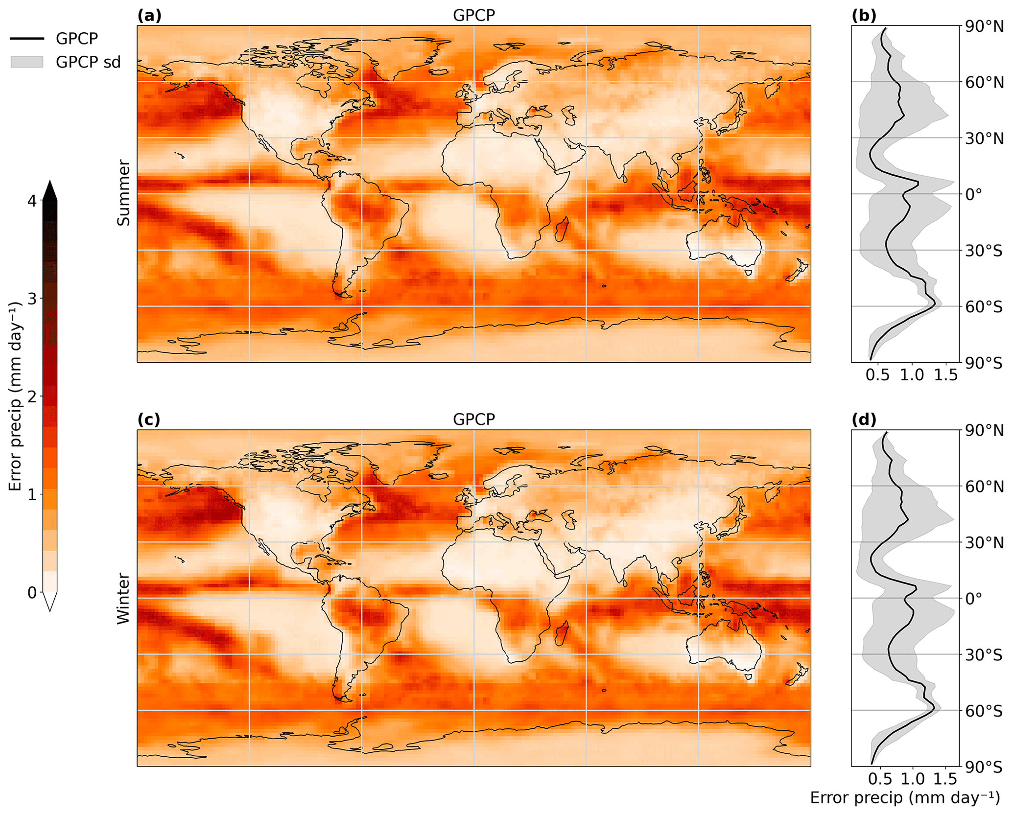
Figure A1 GPCP precipitation error during Northern Hemispheric (NH) summer (a) and NH winter (c) months, with data averaged over the years 2000 to 2010. Additionally, the zonal average of summer (b) and winter (d) months is shown. The shaded area within the zonal mean plot illustrates the standard deviations along longitudes.

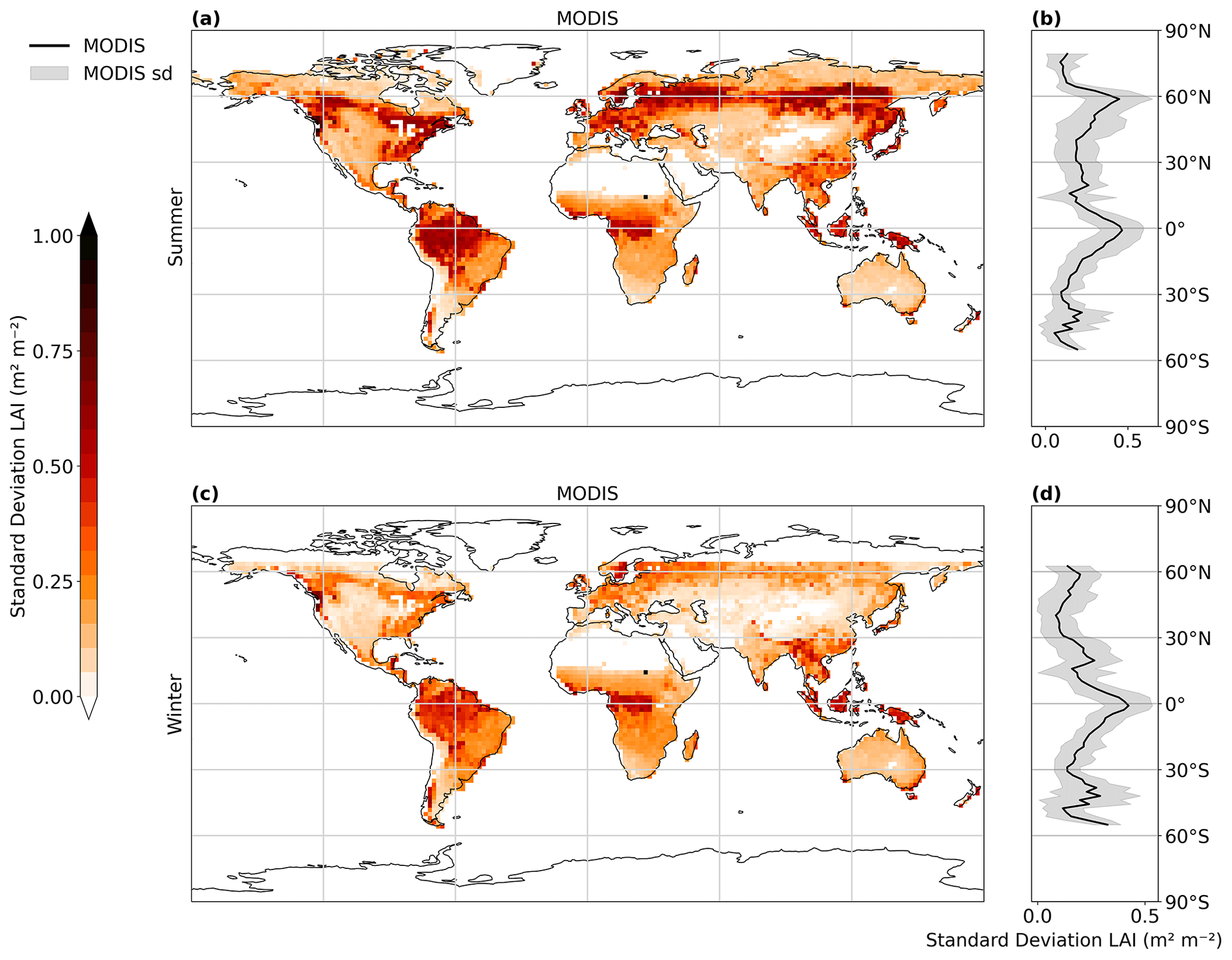
Figure A2 MODIS standard deviation of the leaf area index (LAI) during Northern Hemispheric (NH) summer (a) and NH winter (c) months, with data averaged over the years 2000 to 2010. Additionally, the zonal average of summer (b) and winter (d) months is shown. The shaded area within the zonal mean plot illustrates the standard deviations along longitudes.

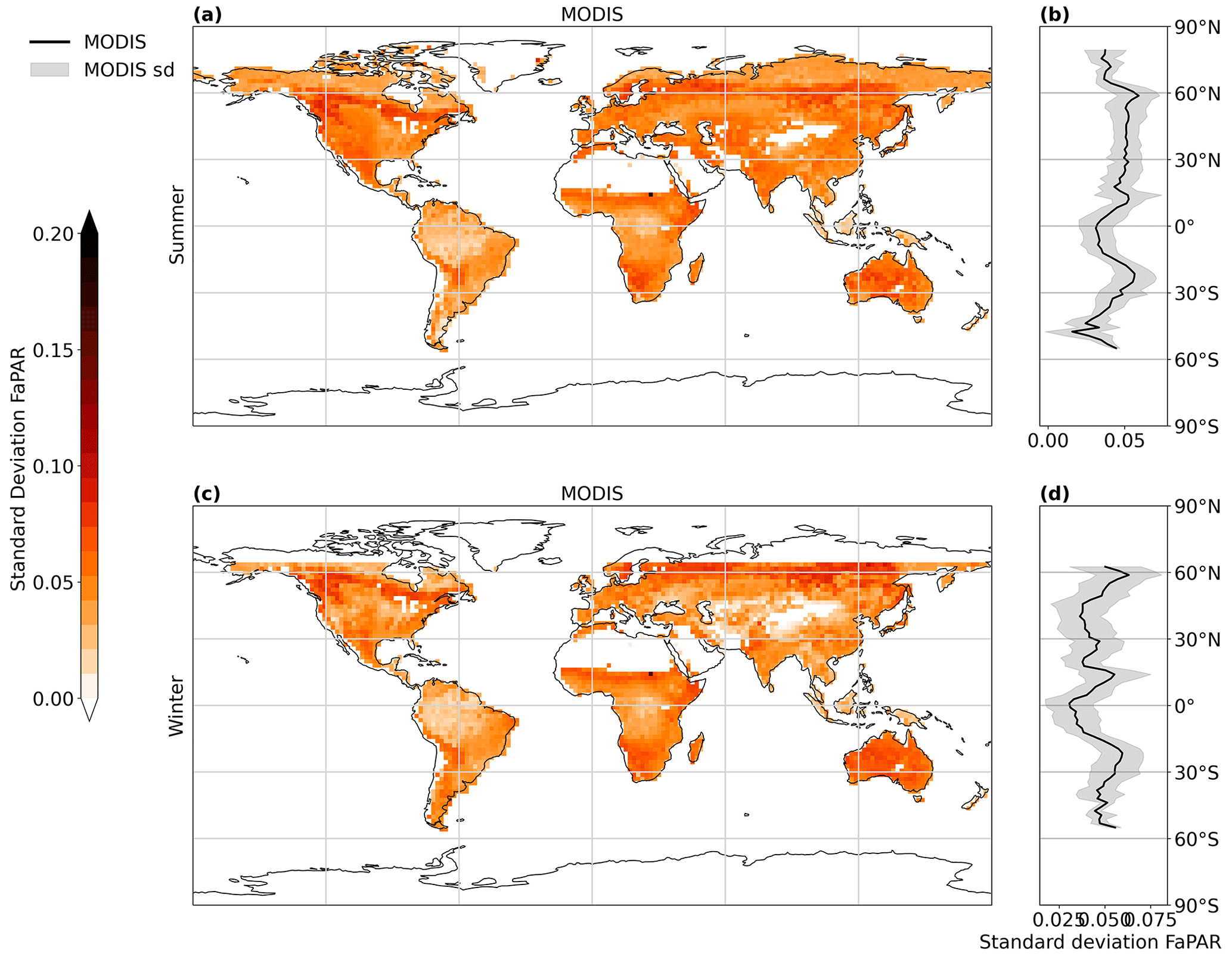
Figure A3 MODIS standard deviation of the fraction of absorbed photosynthetic active radiation (FAPAR) during Northern Hemispheric (NH) summer (a) and NH winter (c) months, with data averaged over the years 2000 to 2010. Additionally, the zonal average of summer (b) and winter (d) months is shown. The shaded area within the zonal mean plot illustrates the standard deviations along longitudes.

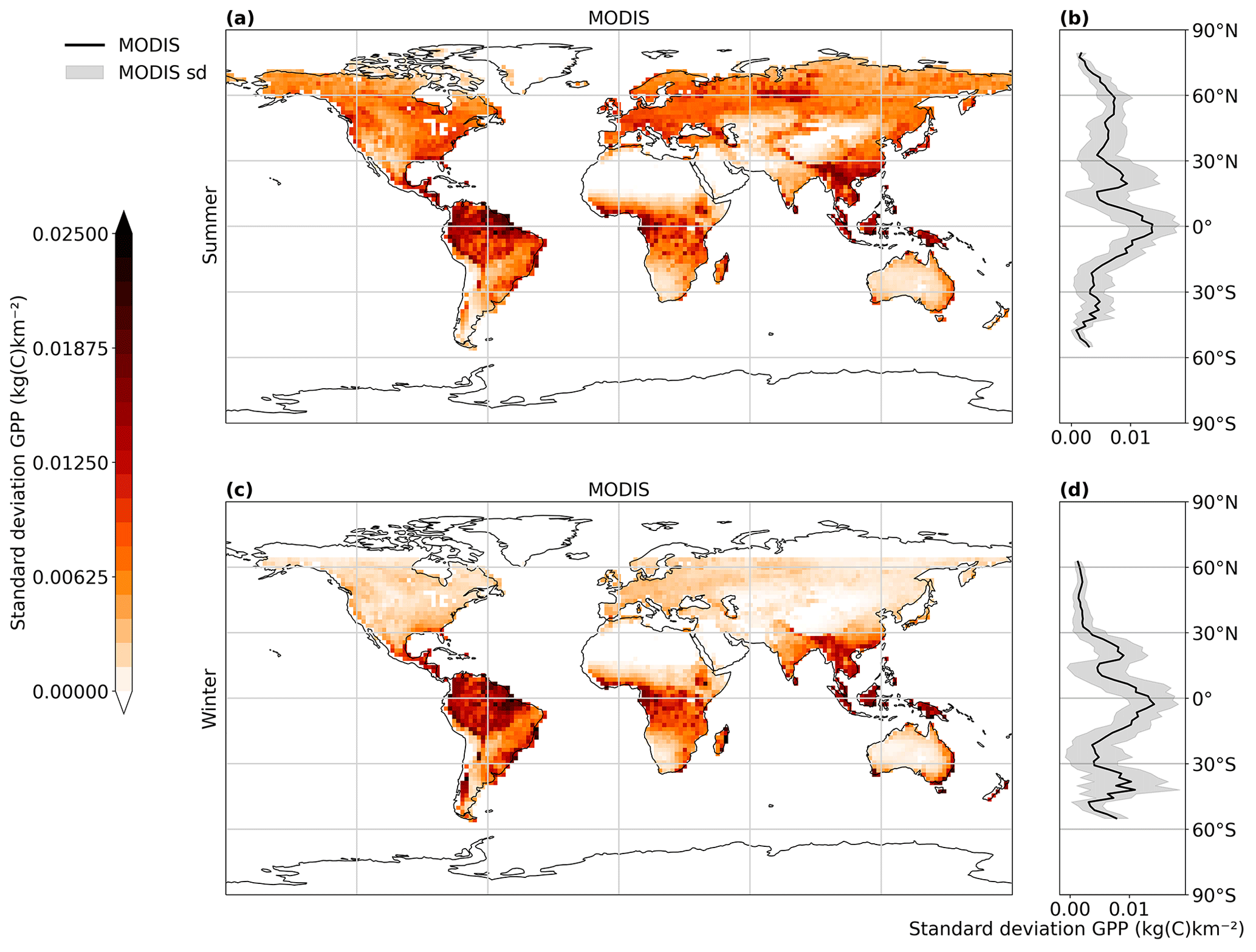
Figure A4 MODIS standard deviation of the gross primary productivity (GPP) during Northern Hemispheric (NH) summer (a) and NH winter (c) months, with data averaged over the years 2000 to 2010. Additionally, the zonal average of summer (b) and winter (d) months is shown. The shaded area within the zonal mean plot illustrates the standard deviations along longitudes.