The first application of a numerically exact, higher-order sensitivity analysis approach for atmospheric modelling: implementation of the hyperdual-step method in the Community Multiscale Air Quality Model (CMAQ) version 5.3.2

Sensitivity analysis in chemical transport models quantifies the response of output variables to changes in input parameters. This information is valuable for researchers engaged in data assimilation and model development. Additionally, environmental decision-makers depend upon these expected responses of concentrations to emissions when designing and justifying air pollution control strategies. Existing sensitivity analysis methods include the finite-difference method, the direct decoupled method (DDM), the complex variable method, and the adjoint method. These methods are either prone to significant numerical errors when applied to nonlinear models with complex components (e.g. finite difference and complex step methods) or difficult to maintain when the original model is updated (e.g. direct decoupled and adjoint methods). Here, we present the implementation of the hyperdual-step method in the Community Multiscale Air Quality Model (CMAQ) version 5.3.2 as CMAQ-hyd. CMAQ-hyd can be applied to compute numerically exact first- and second-order sensitivities of species concentrations with respect to emissions or concentrations. Compared to CMAQ-DDM and CMAQ-adjoint, CMAQ-hyd is more straightforward to update and maintain, while it remains free of subtractive cancellation and truncation errors, just as those augmented models do. To evaluate the accuracy of the implementation, the sensitivities computed by CMAQ-hyd are compared with those calculated with other traditional methods or a hybrid of the traditional and advanced methods. We demonstrate the capability of CMAQ-hyd with the newly implemented gas-phase chemistry and biogenic aerosol formation mechanism in CMAQ. We also explore the cross-sensitivity of monoterpene nitrate aerosol formation to its anthropogenic and biogenic precursors to show the additional sensitivity information computed by CMAQ-hyd. Compared with the traditional finite difference method, CMAQ-hyd consumes fewer computational resources when the same sensitivity coefficients are calculated. This novel method implemented in CMAQ is also computationally competitive with other existing methods and could be further optimized to reduce memory and computational time overheads.

1 Introduction

Ambient air pollution, including particulate matter (PM), poses significant threats to human health. According to the Global Burden of Disease study, among all risk factors, ambient PM pollution accounted for 4.7 % of the disability-adjusted life years (Murray et al., 2020) and over 4.1 million deaths (Fuller et al., 2022) in 2019. Therefore, understanding the complex physicochemical and atmospheric transport processes that lead to PM formation is essential to reducing PM and other harmful secondary atmospheric pollutants. Amongst atmospheric scientists, chemical transport models (CTMs) have become essential tools for interpreting observations of and examining inferences about formation processes of atmospheric pollutants. By solving the mass conservation equation for different species based on atmospheric dispersion and transport, photochemical processes, atmospheric chemistry, and aerosol processes, CTMs can provide estimates of primary and secondary air pollutants (Seinfeld and Pandis, 2016). Environmental decision-makers and researchers rely on CTMs to determine appropriate policies to control air pollution and predict atmospheric pollutant concentrations. Experimental studies (e.g. Ng et al., 2008) and measurement campaigns (e.g. Sareen et al., 2016) provide researchers with more insights about the anthropogenic and biogenic aerosol formation processes. These studies ultimately lead to developments and updates to the gas-phase chemistry and aerosol formation mechanisms in CTMs. For these newly added species and mechanisms in CTMs, understanding the sensitivity of aerosol species concentrations to emissions of their precursors is crucial for determining the priority of primary pollutant emission reductions to achieve atmospheric pollutant reduction objectives.

Sensitivity analysis methods have become invaluable for evaluating uncertainties, understanding concentration–emission relationships in CTMs, and assimilating observations of atmospheric pollutants to improve model parameters. Specifically, the kind of sensitivities described here are the partial derivative of one or more model outputs with respect to one or more model inputs. For instance, if the model has input variables X and output variables Y, the nth-order sensitivity coefficient of one output variable Y_i to one input variable X_i can be represented as the nth-order partial derivative of Y_i with respect to X_i, $\frac{{\partial }^n{Y}_i}{\partial X_i^n}$ (Cohan and Napelenok, 2011). Most sensitivity analysis techniques are formulations of the tangent linear model, which provides source-oriented sensitivities or, mathematically, one column of the Jacobian or Hessian at the model state. In contrast, the model adjoint provides receptor-oriented sensitivities or, mathematically, one row of the Jacobian at the model state. Two distinct approaches to developing these models are the continuous approach, in which the derivative of the underlying equation is formulated and then implemented numerically, and the discrete approach, in which the derivative of the numerical solution of the model is formulated (Sandu et al., 2005). Since the model adjoint provides source-oriented sensitivities and is not directly comparable with other methods (including the hyperdual-step method, which is the focus of this work), it will not be further discussed in the following sections. Other augmented model methods, including the Integrated Source Apportionment Method (Kwok et al., 2013, 2015), are based on a different approach and are thus also not discussed further in the following paragraphs.

The first-order sensitivity coefficient is usually the most useful for CTM applications because it describes the linear relationship between X_i and Y_i. Higher-order sensitivities can be helpful when assessing the nonlinear relationships or dynamics among multiple input variables. Previous studies found that highly nonlinear concentration–emission responses commonly exist in CTMs, particularly for the formation process of PM (Hakami, 2004; Xu et al., 2018; Tian et al., 2010). Therefore, accurately determining the first-order and second-order relationships is useful for understanding concentration–emission responses in CTMs. Practically, the characteristics of an ideal sensitivity analysis method are numerical accuracy, computational efficiency, and minimal development (Lantoine et al., 2012).

Because analytical sensitivities are impractical for these models, researchers have employed a few numerical methods to calculate the first- and higher-order sensitivities in CTMs. One such method is the finite difference method (FDM), which is often designated the brute-force method. The FDM is based on the first- or higher-order approximation of the Taylor series expansion from a small perturbation (Boole, 1960). The sensitivities are calculated by running the model multiple times with incrementally different values for the input variables of interest and taking the difference in the resulting concentration fields. While this method is simple to understand and implement, truncation and subtractive cancellation errors can substantially reduce the accuracy of the calculated sensitivity coefficients, particularly for nonlinear input–output relationships (Fornberg, 1981). Truncation errors originate from neglected higher-order terms in the Taylor series expansion. For instance, suppose a policymaker is interested in calculating the effects of reducing SO₂ emission on the total PM_2.5 concentration. The sensitivity analysis indicates that the first-order partial derivative is positive and the second-order partial derivative is negative. In that case, only considering the first-order FDM approximation will overestimate the effect of reducing the SO₂ emission on the total PM_2.5 concentration. The truncation error can be minimized by taking a small perturbation step, thus eliminating the impact of higher-order sensitivity terms on the first-order result. However, smaller perturbation steps might lead to subtractive cancellation errors, which stem from the fact that computers cannot distinguish two numbers close to each other. If the perturbation size is within the numerical noise of the model, the numerator difference sometimes approaches zero or the sensitivity information might be meaningless, which causes an inherent tension between reducing the truncation error and the subtractive cancellation error for the FDM. Determining ideal perturbation sizes for different variables is challenging because the ideal perturbation size depends on the input species of interest and other parameters in the model. The necessity of selecting the proper perturbation size for each input variable of interest and running the model multiple times makes the FDM a computationally expensive method to obtain sufficiently accurate sensitivities from CTMs.

As a continuous, source-oriented approach, the decoupled direct method (DDM) eliminates the numerical accuracy issues of the FDM and improves the computational efficiency of calculating source-oriented sensitivities but only with a hefty development cost. Dunker (1981) introduced to atmospheric modelling the direct method, which involves formulating new sensitivity equations from the original model and solving both sets simultaneously. The direct method has been proven numerically unstable for solving stiff equations, which exist in many chemical transport models. On the other hand, DDM formulates sensitivity equations like the direct method but separately solves the original and sensitivity equations. This approach improves the computational efficiency and stability compared to the direct method. Yang et al. (1997) was the first to apply the DDM-3D method in a three-dimensional chemical transport model. Hakami et al. (2003) extended the method to a higher-order DDM (HDDM) in the gas phase of the Community Multiscale Air Quality Model (CMAQ), while Zhang et al. (2012) augmented CMAQ-HDDM to include the second-order sensitivities of PM_2.5 concentration to NO_x and SO₂ emissions. Unlike the FDM, the DDM does not incur truncation or subtractive cancellation errors since separate equations are solved for the sensitivities. The DDM also allows the computation of sensitivities of many outputs to more than one input simultaneously, saving significant computation resources. The major disadvantage of DDM for CMAQ and other CTMs is the difficulty of co-development alongside ongoing scientific model development, which is one purpose of CTMs. The implementation of DDM requires writing sensitivity equations for nonlinear steps, which commonly exist in the chemistry and advection parts of CTMs (Fike and Alonso, 2011). New sensitivity equations must be written when CTMs are updated, reducing the ease of maintenance of DDM in complex CTMs and eliminating the opportunity for sensitivities to be used for evaluation in the process of developing new scientific modules within the CTMs.

The complex variable method (CVM) and the multicomplex step approach (MCX) are the methods most comparable to the hyperdual step method. Lyness and Moler (1967) introduced the concept of using imaginary space to propagate derivatives for functions in real space based on Cauchy integrals. Squire and Trapp (1998) made the idea practical through an elegant truncation of the Taylor series expansion of complex numbers which allows nearly exact first-order sensitivities if the imaginary perturbation is small enough. Constantin and Barrett (2014) applied the CVM on the adjoint method of the global CTM GEOS-Chem to compute near-exact sensitivities with receptor orientation in one order and source orientation in the other. Lantoine et al. (2012) developed a multicomplex number system to allow higher-order sensitivities to be calculated to machine precision for functions in real space. Berman et al. (2023) implemented MCX in the inorganic aerosol thermodynamic model ISORROPIA, which is used in CMAQ and other air quality models. These methods require the inclusion of a library of overloaded operators to treat the types of numbers required and the conversion of the model from real to complex space. The accuracy of these approaches is only limited by ensuring that the imaginary perturbation is small enough, which may require tuning depending on the complexity of the model. CVM does not require as much memory and computational time as MCX, but both contribute overhead. Both are very easily updated with new scientific modules. The main limitation of CVM and MCX is that sensitivities cannot be propagated through models, like CMAQ, that originally include calculations in imaginary space.

Finally, the method of interest in this work is the hyperdual-step method (HYD), which computes source-oriented first- and second-order sensitivities to machine precision. HYD relies on hyperdual numbers, which are a specific type of generalized complex number developed particularly for first- and second-order derivative calculations (Fike and Alonso, 2011). The HYD, like the CVM or MCX, is an approach based on a Taylor series expansion in a non-real number space. The unique mathematical properties of hyperdual numbers lead to an elegant calculation of first-, second-, and potentially higher-order sensitivities to machine precision without truncation or cancellation errors. Hyperdual numbers have been applied in numerical models in different fields of study to calculate exact first- and second-order derivatives. Cohen and Shoham (2015) applied hyperdual numbers to compute second-order derivatives in multibody kinetics problems. Tanaka et al. (2015) utilized hyperdual numbers to automatically differentiate hyperelastic material models. Rehner and Bauer (2021) applied hyperdual numbers to equation of state modelling and the calculation of critical points. This method, which is applicable to models with calculations in imaginary space, is accurate to machine precision, reasonably computationally expensive, and quite straightforward to update.

Here, we implement the HYD in CMAQ version 5.3.2 to develop the novel augmented model CMAQ-hyd, and we apply it to calculate the sensitivities of both inorganic and organic aerosol concentrations to their precursor emissions. To our best knowledge, this work represents the first implementation of hyperdual numbers to calculate first- and second-order sensitivities in a CTM. In Sect. 2, hyperdual numbers and the hyperdual-step method are introduced, as is the process of implementing and evaluating HYD in CMAQ. In Sect. 3, the evaluation of first- and second-order sensitivities from CMAQ-hyd is conducted, including the computational costs. In Sect. 4, CMAQ-hyd is applied to understand the influences of anthropogenic and biogenic emissions on select secondary organic aerosol (SOA) concentrations. This work provides an accurate and easily manageable method to compute first- and second-order sensitivities implemented in CMAQ version 5.3.2 and an example of its potential application in other complex models where the sensitivities are of interest.

2 Methods

2.1 Hyperdual numbers and the hyperdual-step method

A hyperdual number (Fike and Alonso, 2011) has four components and is characterized by

$$\begin{array}{}\text{(1)}& H=a_{\mathrm{0}}+a_{\mathrm{1}}{\mathit{ϵ}}_{\mathrm{1}}+a_{\mathrm{2}}{\mathit{ϵ}}_{\mathrm{2}}+a_{\mathrm{12}}{\mathit{ϵ}}_{\mathrm{12}},\end{array}$$

where a₀, a₁, a₂, and a₁₂ are real numbers and ϵ₁, ϵ₂, and ϵ₁₂ are non-real parts. The three crucial properties which enable numerically exact first- and second-order sensitivity calculations are

$$\begin{array}{}\text{(2)}& {\displaystyle }{\mathit{ϵ}}_{\mathrm{1}}^{\mathrm{2}}={\mathit{ϵ}}_{\mathrm{2}}^{\mathrm{2}}={\mathit{ϵ}}_{\mathrm{12}}^{\mathrm{2}}=\mathrm{0}\text{(3)}& {\displaystyle }{\mathit{ϵ}}_{\mathrm{1}}\ne {\mathit{ϵ}}_{\mathrm{2}}\ne {\mathit{ϵ}}_{\mathrm{12}}\ne \mathrm{0}\text{(4)}& {\displaystyle }{\mathit{ϵ}}_{\mathrm{1}}{\mathit{ϵ}}_{\mathrm{2}}={\mathit{ϵ}}_{\mathrm{12}}.\end{array}$$

The squares of the non-real individual parts equal zero (Eq. 2). The non-real parts themselves do not equal anything in real space (Eq. 3). The multiplication of ϵ₁ and ϵ₂ is equal to the third non-real component ϵ₁₂ (Eq. 4). The addition and multiplication of hyperdual numbers are commutative, and the definitions help eliminate the higher-order terms in a Taylor series expansion. A demonstration of several basic operations is provided in the Supplement, while a more detailed discussion of the mathematical properties of hyperdual numbers is given by Fike and Alonso (2011).

Akin to the Taylor series expansion about the real value of x in the finite difference method, the method of ascertaining sensitivities through a perturbation in hyperdual space is based on a Taylor series expansion in an orthogonal dimension of the number. Specifically, a hyperdual number with unity in a₀ and unity in one of a₁ or a₂ is multiplied by the independent variable of interest. After model execution, a Taylor series expansion is applied to extract sensitivities. For instance, the hyperdual-step method is applied to a scalar function f(x) by multiplying x by the hyperdual number $H_{\mathrm{h}}=\mathrm{1.0}+h_{\mathrm{1}}{\mathit{ϵ}}_{\mathrm{1}}+h_{\mathrm{2}}{\mathit{ϵ}}_{\mathrm{2}}$, which results in

$$\begin{array}{}\text{(5)}& \begin{array}{rl}f\left(x{H}_{\mathrm{h}}\right)=& f\left(x\right)+(x{h}_{\mathrm{1}}{\mathit{ϵ}}_{\mathrm{1}}+x{h}_{\mathrm{2}}{\mathit{ϵ}}_{\mathrm{2}})f^{\prime }\left(x\right)+{\displaystyle \frac{\mathrm{1}}{\mathrm{2}\mathrm{!}}}\\ & \times (x{h}_{\mathrm{1}}{\mathit{ϵ}}_{\mathrm{1}}+x{h}_{\mathrm{2}}{\mathit{ϵ}}_{\mathrm{2}}{)}^{\mathrm{2}}{f}^{\prime \prime }(x)\\ & +{\displaystyle \frac{\mathrm{1}}{\mathrm{3}\mathrm{!}}}(x{h}_{\mathrm{1}}{\mathit{ϵ}}_{\mathrm{1}}+x{h}_{\mathrm{2}}{\mathit{ϵ}}_{\mathrm{2}}{)}^{\mathrm{3}}{f}^{\prime \prime \prime }(x)+\mathrm{\dots },\end{array}\end{array}$$

where “…” represents higher-order terms in the series. Eliminating all terms that are zero due to the definition of hyperdual numbers (Eq. 2) leads to

$$\begin{array}{}\text{(6)}& \begin{array}{rl}f\left(x{H}_{\mathrm{h}}\right)=& f\left(x\right)+(x{h}_{\mathrm{1}}{\mathit{ϵ}}_{\mathrm{1}}+x{h}_{\mathrm{2}}{\mathit{ϵ}}_{\mathrm{2}})f^{\prime }\left(x\right)\\ & +x^{\mathrm{2}}{h}_{\mathrm{1}}{h}_{\mathrm{2}}{\mathit{ϵ}}_{\mathrm{12}}{f}^{\prime \prime }\left(x\right),\end{array}\end{array}$$

where f(xH_h) is a hyperdual number.

The properties of hyperdual numbers (Eqs. 2–4) lead to two significant results. First, all terms in the Taylor series expansion with derivatives higher than second order become zero because all values include ${\mathit{ϵ}}_{\mathrm{1}}^{\mathrm{2}}$, ${\mathit{ϵ}}_{\mathrm{2}}^{\mathrm{2}}$, or ${\mathit{ϵ}}_{\mathrm{12}}^{\mathrm{2}}$. Second, the real component is unchanged. A more detailed expansion of terms can be found in Eq. (S7) in the Supplement or the original development of hyperdual numbers; it follows the multiplication rule between a hyperdual and a real number (Fike and Alonso, 2011). Finally, the first- and second-order derivatives are separated into different parts of the hyperdual number. The first-order derivative exists in either the ϵ₁ or the ϵ₂ term, while the second-order derivatives only exist in the ϵ₁₂ term. The first- and second-order derivatives are

$$\begin{array}{}\text{(7)}& {\displaystyle }{f}^{\prime }\left(x\right)={\displaystyle \frac{{\mathit{ϵ}}_{\mathrm{1}}\mathrm{part}\left[f\left(x{H}_{\mathrm{h}}\right)\right]}{x{h}_{\mathrm{1}}}}={\displaystyle \frac{{\mathit{ϵ}}_{\mathrm{2}}\mathrm{part}\left[f\left(x{H}_{\mathrm{h}}\right)\right]}{x{h}_{\mathrm{2}}}}\text{(8)}& {\displaystyle }{f}^{\prime \prime }\left(x\right)={\displaystyle \frac{{\mathit{ϵ}}_{\mathrm{12}}\mathrm{part}\left[f\left(x{H}_{\mathrm{h}}\right)\right]}{x^{\mathrm{2}}{h}_{\mathrm{1}}{h}_{\mathrm{2}}}},\end{array}$$

where ϵ₁part[], ϵ₂part[], and ϵ₁₂part[] represent functions that extract the a₁, a₂, or a₁₂, respectively. Since the derivative computation process (Eqs. 6–9) does not involve subtractions or higher-order sensitivities, the first- and second-order sensitivities calculated by the hyperdual-step method are free from subtractive cancellation and truncation errors. This method (Eqs. 8 and 9) extends to vector operations to compute arrays of numerically exact derivatives. For instance, the partial first- and second-order derivatives for f(x), where $\mathit{x}=[x_{\mathrm{1}},x_{\mathrm{2}},\mathrm{\dots },x_n]$, with respect to x₁ through a hyperdual-step perturbation to x₁ is

$$\begin{array}{}\text{(9)}& {\displaystyle \frac{\partial f\left(\mathit{x}\right)}{\partial x_{\mathrm{1}}}}={\displaystyle \frac{{\mathit{ϵ}}_{\mathrm{1}}\mathrm{part}\left[f\right(\mathit{x}{H}_{h,x_{\mathrm{1}}}\left)\right]}{x_{\mathrm{1}}{h}_{\mathrm{1}}}}={\displaystyle \frac{{\mathit{ϵ}}_{\mathrm{2}}\mathrm{part}\left[f\right(\mathit{x}{H}_{h,x_{\mathrm{1}}}\left)\right]}{x_{\mathrm{1}}{h}_{\mathrm{2}}}}\text{(10)}& {\displaystyle \frac{{\partial }^{\mathrm{2}}f\left(\mathit{x}\right)}{\partial x_{\mathrm{1}}^{\mathrm{2}}}}={\displaystyle \frac{{\mathit{ϵ}}_{\mathrm{12}}\mathrm{part}\left[f\right(\mathit{x}{H}_{h,x_{\mathrm{1}}}\left)\right]}{x_{\mathrm{1}}^{\mathrm{2}}{h}_{\mathrm{1}}{h}_{\mathrm{2}}}}.\end{array}$$

Similarly, two different independent variables x₁ and x₂ may be perturbed simultaneously. In this case, two arrays of first-order sensitivity and one array of cross-sensitivity result:

$$\begin{array}{}\text{(11)}& {\displaystyle \frac{\partial f\left(\mathit{x}\right)}{\partial x_{\mathrm{1}}}}={\displaystyle \frac{{\mathit{ϵ}}_{\mathrm{1}}\mathrm{part}\left[f\right(\mathit{x}{H}_{\mathrm{h}}\left)\right]}{x_{\mathrm{1}}{h}_{\mathrm{1}}}}\text{(12)}& {\displaystyle \frac{\partial f\left(\mathit{x}\right)}{\partial x_{\mathrm{2}}}}={\displaystyle \frac{{\mathit{ϵ}}_{\mathrm{2}}\mathrm{part}\left[f\right(\mathit{x}{H}_{\mathrm{h}}\left)\right]}{x_{\mathrm{2}}{h}_{\mathrm{2}}}}\text{(13)}& {\displaystyle \frac{{\partial }^{\mathrm{2}}f\left(\mathit{x}\right)}{\partial x_{\mathrm{1}}\partial x_{\mathrm{2}}}}={\displaystyle \frac{{\mathit{ϵ}}_{\mathrm{12}}\mathrm{part}\left[f\right(\mathit{x}{H}_{\mathrm{h}}\left)\right]}{x_{\mathrm{1}}{x}_{\mathrm{2}}{h}_{\mathrm{1}}{h}_{\mathrm{2}}}}.\end{array}$$

Therefore, the two variations of the hyperdual-step method will generate either one or two arrays of first-order sensitivities and one array of second-order or cross sensitivities with a single run of the model.

2.2 Community Multiscale Air Quality Model and the implementation of the hyperdual-step method

The Community Multiscale Air Quality Model (CMAQ), developed by the U.S. Environmental Protection Agency (EPA), is an Eulerian CTM which can predict air pollutant concentrations at regional and hemispheric scales (Byun and Schere, 2006). CMAQ represents advection, diffusion, gas-phase chemistry, aerosol processes, cloud processes, and photolysis. CMAQ has been applied to predict pollutant concentrations in the atmosphere (Liu et al., 2010; Sayeed et al., 2021), understand fundamental atmospheric chemistry and aerosol formation mechanisms (Zhu et al., 2018; Li et al., 2019), and guide policy-making processes (Chemel et al., 2014; Che et al., 2011; Li et al., 2019; Ring et al., 2018). CMAQ is used in the regulatory process of the US EPA when states, tribes, or local jurisdictions demonstrate how they will attain the National Ambient Air Quality Standard (NAAQS) and or comply with the Regional Haze Rule (Mebust et al., 2003). CMAQ solves the atmospheric diffusion equation shown in Eq. (14) to calculate the concentrations of gaseous and aerosol species in the atmosphere:

$$\begin{array}{}\text{(14)}& {\displaystyle \frac{\partial c_i}{\partial t}}=-\mathrm{\nabla }\left(\mathit{u}{c}_i\right)+\mathrm{\nabla }\left(K\mathrm{\nabla }{c}_i\right)+R_i+E_i,\end{array}$$

where c_i, u, K, R_i, and E_i are the concentration of species i, the wind velocity vector, the diffusivity tensor, the change in concentration due to chemical reactions of species i, and the emission rate of species i, respectively. Species concentrations are stored in a multidimensional array and propagated through different scientific modules within the model. For this work, CMAQ was run with 12 km by 12 km horizontal resolution and with 35 vertical layers, 100 columns, and 80 rows over the Southeast US on 1 July 2016, GMT (U.S. Environmental Protection Agency, 2019). The gas-phase chemistry mechanism used is Carbon Bond 6 (Luecken et al., 2019).

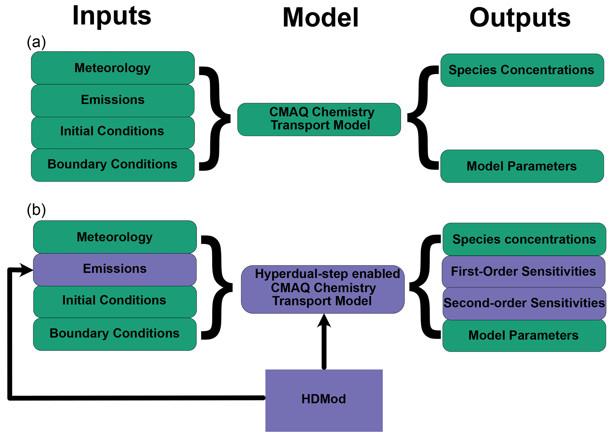
Figure 1 A schematic showing the original CMAQ model compared with CMAQ-hyd. (a) The original CMAQ model (green). (b) The CMAQ-hyd model. CMAQ-hyd incorporates the hyperdual number operator overloading module. The purple components in (b) represent changes made to the original CMAQ model. Changes were made to the modules and emission-processing parts of CMAQ. The first- and second-order sensitivities of species concentrations with respect to selected precursor concentrations or emissions are new outputs of the model.

In CMAQ, the hyperdual-step method was implemented by strategically converting the model to use hyperdual numbers (Fig. 1). First, the operators were overloaded by translating a C-based library from Fike and Alonso (2011) to Fortran (“HDMod”) and augmenting it to treat multidimensional data as required by CMAQ. HDMod, which defines a hyperdual version of all possible calculations related to the chemical concentration array, was developed. The library includes basic arithmetic operations, such as addition and subtraction, as well as more advanced functions like trigonometric functions. Before being applied to CMAQ, the operator overloading library was separately validated by comparing it against analytical derivatives using a testing framework developed by Pellegrini and Russell (2016). Secondly, the CMAQ variable containing species concentration information and all other variables that depend on it were converted from real numbers to the newly defined hyperdual number type. The source code was carefully analysed to select only the necessary variables for conversion. Many variables in CMAQ do not need to be altered because they do not influence the main concentration array. This highly detailed process helped minimize the additional computational burden of the model since calculations with hyperdual numbers are more computationally intensive than those with real numbers. For instance, one hyperdual multiplication operation shown in Eq. (5) results in five more additions and nine more multiplications than an operation with real numbers. According to Fike and Alonso (2011), the computational cost of a hyperdual calculation ranges from 4 to 14 times higher than the original operation. Applying hyperdual numbers to all the variables in a CFD model results in an approximately 10 times higher computational cost (Fike and Alonso, 2011). Thirdly, the first- and second-order sensitivities of the species concentrations to perturbed emissions are included in the new hyperdual array, which is then saved to additional output files using the same structure as the output of the original concentration array. As a result, first- and second-order sensitivities can be propagated through the model without significantly modifying the source code. The modification efforts mainly focused on determining the variables that must be converted to the hyperdual type. Consequently, updating CMAQ-hyd when there are changes to the original model is a simple process that involves converting only the newly added variables to the hyperdual type. This simplicity is an advantage over other computational techniques, such as the DDM and adjoint method, which compute numerically exact sensitivities but require more complex and time-consuming update procedures, including writing new equations.

Several source code alterations were made to reduce the complexity of development and overcome the numerical instabilities related to hyperdual calculations in CMAQ's aerosol module, specifically within the inorganic thermodynamic module ISORROPIA (Fountoukis and Nenes, 2007; Nenes et al., 1998). For the simplicity of development, we applied a Fortran-90-compilant version of ISORROPIA to replace the original Fortran 77 version of ISORROPIA in CMAQ.

ISORROPIA, a key component of the aerosol module in CMAQ, is called in either the forward or the reverse mode. The forward mode of ISORROPIA takes the sum of gas and aerosol species concentrations, along with the relative humidity and temperature, to determine the partitioning of Aitken- and accumulation-mode species across the gas and aerosol phases in CMAQ. In the original CMAQ model, ISORROPIA is run in the forward mode without limiting the temperature and pressure of the simulation. The determination process for species concentrations involves an iterative method which is sometimes numerically unstable during iterations for upper layer cells with low temperature and pressure for sensitivity computations with the HYD. To increase the numerical stability of CMAQ-hyd, we implemented temperature and pressure constraints so that the forward-mode ISORROPIA is only called when the cell temperature exceeds 260 K and the cell pressure exceeds 20 000 Pa. A similar set of temperature and pressure limits were applied to the call of ISORROPIA in the adjoint of CMAQ (Zhao et al., 2020). These changes do not affect the species concentrations computed by CMAQ while ensuring that the sensitivity computation process is stable.

To calculate the dynamic equilibrium of coarse-mode aerosol species with the gas phase (Pilinis et al., 2000; Capaldo et al., 2000), CMAQ employs the reverse mode of ISORROPIA. The input to reverse-mode ISORROPIA includes concentrations of aerosol species, relative humidity, and temperature, and it results in partitioned concentrations in the solid, liquid, and gas phases for coarse-mode inorganic aerosols. The reverse-mode solution leads to unrealistic sensitivities calculated by the HYD when the aerosol pH is close to neutral. One previous study found that the reverse ISORROPIA fails to capture the actual behaviour of inorganic aerosol when the pH is close to 7 (Hennigan et al., 2015). To ensure the stability of the sensitivity calculations, the changes to the hyperdual components in the coarse-mode dynamic equilibrium are ignored when the pH of coarse-mode aerosol is close to neutral, which ensures that the real components are identical to the original model.

2.3 Evaluating sensitivities from CMAQ-hyd

CMAQ-hyd produces sensitivities that can be semi- or fully normalized for concentrations from any range of grid cells and times with respect to emissions or concentrations from any range of grid cells and times. Here, for the sake of illustration, we consider the semi-normalized sensitivities of time-averaged output concentrations of ground-level PM_2.5 concentrations ($C_{{\mathrm{PM}}_{\mathrm{2.5}},c,r,l=\mathrm{0},t}$) to input NO_x (NO + NO₂) emissions ($E_{{\mathrm{NO}}_x,c,r,l,t}$) averaged over time, t, for any given cell as indicated by the column c and row r. The first-order semi-normalized sensitivities, $s_{{\mathrm{NO}}_x}^{{\mathrm{PM}}_{\mathrm{2.5}}}$, and second-order semi-normalized sensitivities, $s_{{\mathrm{NO}}_x}^{\left(\mathrm{2}\right){\mathrm{PM}}_{\mathrm{2.5}}}$, exemplify sensitivities relevant to environmental decision makers (Eqs. 15 and 16).

$$\begin{array}{}\text{(15)}& {\displaystyle }{s}_{{\mathrm{NO}}_x}^{{\mathrm{PM}}_{\mathrm{2.5}}}={\displaystyle \frac{\partial \stackrel{\mathrm{‾}}{C_{{\mathrm{PM}}_{\mathrm{2.5}},c,r,l=\mathrm{0},t}{\mathrm{|}}_t}}{\partial \stackrel{\mathrm{‾}}{E_{{\mathrm{NO}}_x,c,r,l,t}}{\mathrm{|}}_t}}\stackrel{\mathrm{‾}}{E_{{\mathrm{NO}}_x,c,r,l,t}}{\mathrm{|}}_t\text{(16)}& {\displaystyle }{s}_{{\mathrm{NO}}_x}^{\left(\mathrm{2}\right){\mathrm{PM}}_{\mathrm{2.5}}}={\displaystyle \frac{{\partial }^{\mathrm{2}}\stackrel{\mathrm{‾}}{C_{{\mathrm{PM}}_{\mathrm{2.5}},c,r,l=\mathrm{0},t}{\mathrm{|}}_t}}{\partial \stackrel{\mathrm{‾}}{E_{{\mathrm{NO}}_x,c,r,l,t}^{\mathrm{2}}}{\mathrm{|}}_t}}\stackrel{\mathrm{‾}}{E_{{\mathrm{NO}}_x,c,r,l,t}^{\mathrm{2}}}{\mathrm{|}}_t\end{array}$$

Semi-normalized sensitivities reduce the complexity of interpretation by providing sensitivities in the units of concentration per percent change of emissions. The semi-normalized sensitivities also scale down the impact from cells with low emission rates, which is consistent with the concentration reduction that is realistic to expect. Similarly, the time-averaged, semi-normalized cross-sensitivity of PM_2.5 to both NO_x and monoterpene is denoted as $s_{{\mathrm{NO}}_x,\mathrm{TERP}}^{\left(\mathrm{2}\right){\mathrm{PM}}_{\mathrm{2.5}}}$, with E_TERP representing the emission of monoterpenes (Eq. 17).

$$\begin{array}{}\text{(17)}& \begin{array}{rl}{s}_{{\mathrm{NO}}_x,\mathrm{TERP}}^{\left(\mathrm{2}\right){\mathrm{PM}}_{\mathrm{2.5}}}=& {\displaystyle \frac{{\partial }^{\mathrm{2}}\stackrel{\mathrm{‾}}{C_{{\mathrm{PM}}_{\mathrm{2.5}},c,r,l=\mathrm{0},t}}{\mathrm{|}}_t}{\partial \stackrel{\mathrm{‾}}{E_{{\mathrm{NO}}_x,c,r,l,t}}{\mathrm{|}}_t\stackrel{\mathrm{‾}}{E_{\mathrm{TERP},c,r,l,t}}{\mathrm{|}}_t}}\\ & \times \stackrel{\mathrm{‾}}{E_{{\mathrm{NO}}_x,c,r,l,t}}{\mathrm{|}}_t\stackrel{\mathrm{‾}}{E_{\mathrm{TERP},c,r,l,t}}{\mathrm{|}}_t\end{array}\end{array}$$

The evaluation of the first order sensitivities of CMAQ-hyd is done by performing a comparison of the sensitivities calculated by the hyperdual-step method against those from the FDM (Eq. 18). The comparison is illustrated with an example of calculating cell-specific sensitivities of PM_2.5 concentration to NO_x emissions. The first-order sensitivity of PM_2.5 concentration at the end of a 24 h simulation to a cumulative NO_x emission perturbation is given by

$$\begin{array}{}\text{(18)}& \begin{array}{rl}& s_{{\mathrm{NO}}_x}^{{\mathrm{PM}}_{\mathrm{2.5}},t=\mathrm{24}}\\ \approx & {\displaystyle \frac{C_{{\mathrm{PM}}_{\mathrm{2.5}},c,r,l,t=\mathrm{24}}^{\text{inc}}-C_{{\mathrm{PM}}_{\mathrm{2.5}},c,r,l,t=\mathrm{24}}^{\text{dec}}}{{\sum }_{t=\mathrm{0}}^{t=\mathrm{24}}{E}_{{\mathrm{NO}}_x,c,r,l=\mathrm{0},t}^{\text{inc}}-{\sum }_{t=\mathrm{0}}^{t=\mathrm{24}}{E}_{{\mathrm{NO}}_x,c,r,l=\mathrm{0},t}^{\text{dec}}}}\\ & \times {\mathrm{\Sigma }}_{t=\mathrm{0}}^{t=\mathrm{24}}{E}_{{\mathrm{NO}}_x,c,r,l=\mathrm{0},t}^{\text{orig}},\end{array}\end{array}$$

where the subscripts c, r, and l represent the column, row, and layer; the subscript t represents the time from the start of the model run; and the superscripts “inc”, “dec”, and “orig” represent the initial perturbation direction (i.e. increased, decreased, and original emissions, respectively). For instance, $C_{{\mathrm{PM}}_{\mathrm{2.5}},c,r,l,t=\mathrm{24}}^{\text{inc}}$ is the concentration of PM_2.5 for each column, row, and layer 24 h into the run when there is an increase in NO_x emissions throughout the model run. Unless otherwise noted, the relative perturbation sizes for first-order FDM calculations are 125 % and 75 % for domain-wide emissions. The average ground-layer sensitivities for the 24 h simulation time are computed. Previous studies have found that smaller perturbation sizes for inorganic aerosol sensitivity calculations in CMAQ using FDM are more prone to numerical noise (Zhang et al., 2012). The semi-normalized sensitivity of each cell is computed with the central difference method and is only an approximation of the actual sensitivity due to subtractive cancellation and truncation errors. The numerator is the difference between PM_2.5 concentrations with persistent increases or decreases in NO_x emissions. The denominator is the total emission perturbation of NO_x emission. The sensitivities are semi-normalized by the sum of the NO_x emissions in the base model run. The calculated first-order semi-normalized sensitivities will have units of µg m⁻³.

The semi-normalized sensitivity of PM_2.5 concentrations with respect to NO_x emissions using a hyperdual perturbation of $H_{\mathrm{a}}=\mathrm{1}+a_{\mathrm{1}}{\mathit{ϵ}}_{\mathrm{1}}+a_{\mathrm{2}}{\mathit{ϵ}}_{\mathrm{2}}$ is computed by the hyperdual-step method as

$$\begin{array}{}\text{(19)}& \begin{array}{rl}{s}_{{\mathrm{NO}}_x}^{{\mathrm{PM}}_{\mathrm{2.5}},t=\mathrm{24}}& ={\displaystyle \frac{{\mathit{ϵ}}_{\mathrm{1}}\mathrm{part}\left[C_{{\mathrm{PM}}_{\mathrm{2.5}},c,r,l,t=\mathrm{24}}^{\text{orig}}\right]}{a_{\mathrm{1}}}}\\ & ={\displaystyle \frac{{\mathit{ϵ}}_{\mathrm{2}}\mathrm{part}\left[C_{{\mathrm{PM}}_{\mathrm{2.5}},c,r,l,t=\mathrm{24}}^{\text{orig}}\right]}{a_{\mathrm{2}}}}.\end{array}\end{array}$$

The first-order semi-normalized sensitivity can be computed with either the ϵ₁ or the ϵ₂ part. The ϵ₁ or the ϵ₂ part of the PM_2.5 concentration is divided by the initial perturbation in the ϵ₁ or ϵ₂ space, respectively. The emissions in the denominator will cancel out with the semi-normalized emissions.

Although the FDM can be applied to compute second-order sensitivities in CMAQ, previous studies have shown that the results are noisy and highly dependent on the perturbation sizes (Zhao et al., 2020; Zhang et al., 2012). In order to evaluate the second-order sensitivities computed by the HYD method, we adopted a hybrid hyperdual–finite difference method (HYD-FDM). The HYD-FDM sensitivity calculation is given by

$$\begin{array}{}\text{(20)}& \begin{array}{rl}& s_{{\mathrm{NO}}_x}^{\left(\mathrm{2}\right){\mathrm{PM}}_{\mathrm{2.5}}}\\ \approx & {\displaystyle \frac{\frac{{\mathit{ϵ}}_{\mathrm{1}}\mathrm{part}\left[C_{{\mathrm{PM}}_{\mathrm{2.5}},c,r,l,t=\mathrm{24}}^{\text{inc}}\right]}{a_{\mathrm{1}}{\sum }_{t=\mathrm{0}}^{t=\mathrm{24}}{E}_{{\mathrm{NO}}_x,c,r,l=\mathrm{0},t}^{\text{inc}}}-\frac{{\mathit{ϵ}}_{\mathrm{1}}\mathrm{part}\left[C_{{\mathrm{PM}}_{\mathrm{2.5}},c,r,l,t=\mathrm{24}}^{\text{dec}}\right]}{b_{\mathrm{1}}{\sum }_{t=\mathrm{0}}^{t=\mathrm{24}}{E}_{{\mathrm{NO}}_x,c,r,l=\mathrm{0},t}^{\text{dec}}}}{{\sum }_{t=\mathrm{0}}^{t=\mathrm{24}}{E}_{{\mathrm{NO}}_x,c,r,l=\mathrm{0},t}^{\text{inc}}-{\sum }_{t=\mathrm{0}}^{t=\mathrm{24}}{E}_{{\mathrm{NO}}_x,c,r,l=\mathrm{0},t}^{\text{dec}}}}\\ & \times {\left({\mathrm{\Sigma }}_{t=\mathrm{0}}^{t=\mathrm{24}}{E}_{{\mathrm{NO}}_x,c,r,l=\mathrm{0},t}^{\text{orig}}\right)}^{\mathrm{2}},\end{array}\end{array}$$

where two separate simulations were run: one with increased and another with decreased initial NO_x emissions. The emission perturbations for the two runs are $H_{\mathrm{a}}=\mathrm{1}+a_{\mathrm{1}}{\mathit{ϵ}}_{\mathrm{1}}+a_{\mathrm{2}}{\mathit{ϵ}}_{\mathrm{2}}$ for the run with increased initial NO_x emission and $H_{\mathrm{b}}=\mathrm{1}+b_{\mathrm{1}}{\mathit{ϵ}}_{\mathrm{1}}+b_{\mathrm{2}}{\mathit{ϵ}}_{\mathrm{2}}$ for the run with decreased initial emission of NO_x. HYD-FDM uses the regular finite difference on the difference between first-order sensitivities calculated by using the ϵ₁ part of the hyperdual-step results. The sensitivity in this equation is an estimate and subject to numerical errors because it includes the usage of FDM.

The second-order sensitivity calculated by the hyperdual-step method is shown in Eq. (21) below:

$$\begin{array}{}\text{(21)}& s_{{\mathrm{NO}}_x}^{\left(\mathrm{2}\right){\mathrm{PM}}_{\mathrm{2.5}}}={\displaystyle \frac{{\mathit{ϵ}}_{\mathrm{12}}\mathrm{part}\left[C_{{\mathrm{PM}}_{\mathrm{2.5}},c,r,l,t=\mathrm{24}}^{\text{orig}}\right]}{a_{\mathrm{1}}{a}_{\mathrm{2}}}}.\end{array}$$

The hyperdual-step method uses the ϵ₁₂ part of the output variable, dividing it by the multiplication of a₁ and a₂. The second-order sensitivities calculated only by the HYD method are numerically exact. All the sensitivities are computed for each cell, and comparisons between the finite difference and the hyperdual-step method are performed on a cell-to-cell basis.

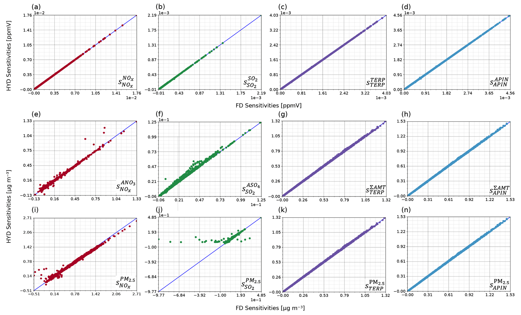
Figure 2 The comparisons of first-order sensitivities on the ground layer calculated by the hyperdual-step method (HYD sensitivities) and FDM (FD sensitivities). The sensitivities are colour coded by the perturbed emissions (i.e. NO_x, SO₂, TERP, and APIN). Panels (a)–(d) show the gas-phase species sensitivities with respect to their emissions. APIN denotes α-pinene and TERP denotes all other monoterpene species. Panels (e)–(h) show examples of aerosol-phase products with respect to their precursors. ANO₃ denotes the total aerosol-phase nitrate products. ASO₄ denotes the total aerosol sulfate products. ΣAMT denotes the total aerosol photooxidation products from monoterpene. Panels (i)–(n) show the total PM_2.5 concentration with respect to gas-phase precursors. The sensitivities calculated are noted at the bottom-right corner of each panel with the notation pattern mentioned in Sect. 2.3.

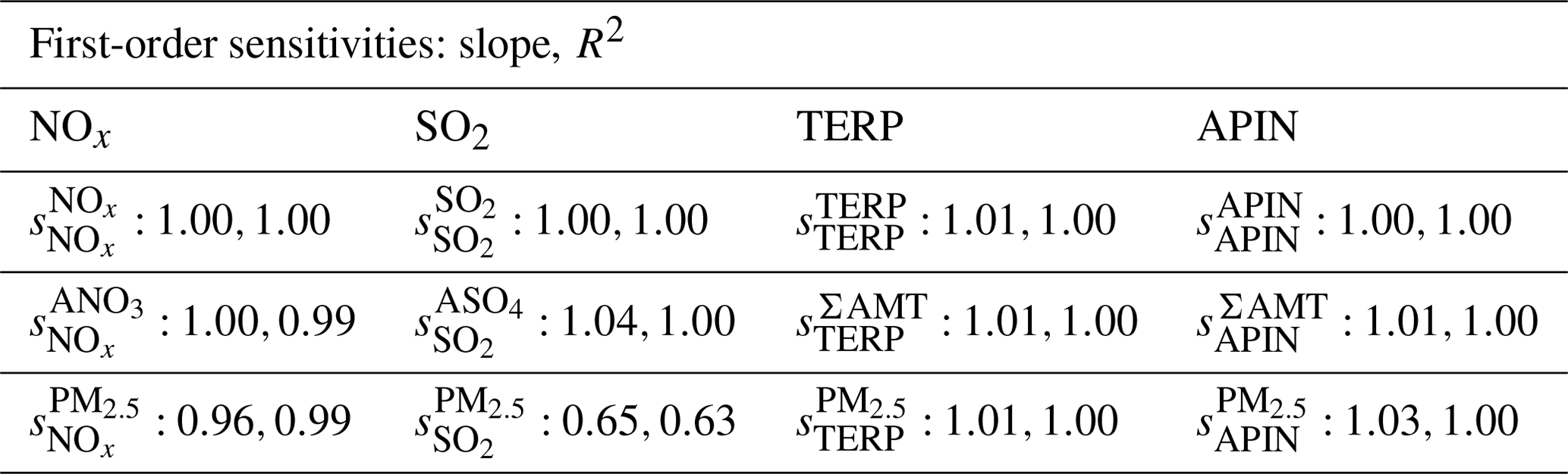
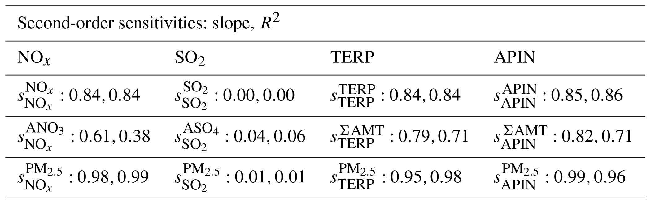
Table 1 The slopes and R² values from the linear regression of the first-order sensitivities of ground-layer species concentrations to domain-wide perturbations by the hyperdual-step method compared to finite-difference sensitivities. The gas-phase species sensitivities with respect to their emissions are on line three, where APIN denotes α-pinene and TERP denotes all other monoterpene species. Line four includes sensitivities of aerosol-phase products with respect to their precursors, where ANO₃ denotes the total aerosol-phase nitrate products, ASO₄ denotes the total aerosol sulfate products, and ΣAMT denotes the total aerosol photooxidation products from monoterpene. Line five includes the sensitivities of the total PM_2.5 concentration with respect to each gas-phase precursor. A visual comparison of the agreement for each relationship is shown in Fig. 2.

3 Results and discussion

3.1 Evaluation of the first- and second-order sensitivities

We evaluated the implementation of CMAQ-hyd by comparing the first-order sensitivities of various species in CMAQ calculated by HYD with a hyperdual-step perturbation as described in Sect. 2.3 (HYD sensitivities) and FDM with a domain-wide emission perturbation (FD sensitivities). The FD sensitivities were computed with the difference between a 25 % increase and a 25 % decrease in domain-wide emissions using the central finite difference method. Overall, the different HYD and FD sensitivities agree well, as evidenced by the close alignment of the points on the blue identity line, which represents perfect agreement, in most of the panels of Fig. 2. The slope and R² values for all comparisons are provided in Table 1, and additional slope and R² values are provided in Tables S1 and S2 in the Supplement. Specifically, the slopes and R² values for gas-phase species concentrations on the ground layer with respect to their emissions on the ground layer (Fig. 2a–d) are all 1.00 (Table 1), indicating minimal nonlinearity in these relationships, as expected.

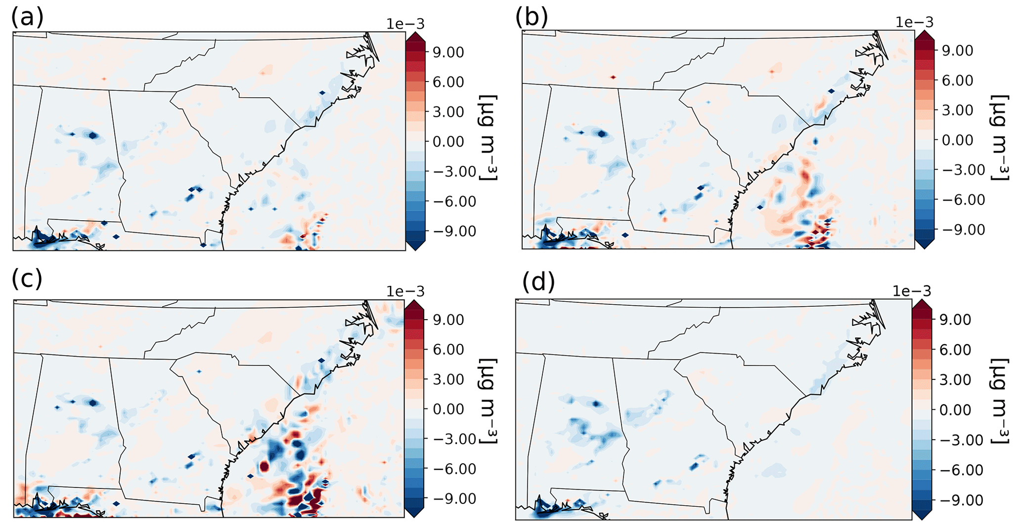
Figure 3 Comparisons of the first-order sensitivities of ground-layer aerosol nitrate (ANO₃) concentration with respect to a domain-wide perturbation of SO₂ emission calculated by the FDM method (a–c) and the HYD method. (a) FD sensitivities calculated with the central difference method and a 25 % perturbation each way (125 %, 75 %). (b) FD sensitivities calculated with the central difference method and a 10 % perturbation each way (110 %, 90 %). (c) FD sensitivities calculated with the central difference method and a 5 % perturbation each way (105 %, 95 %). (d) HYD sensitivities.

Secondary aerosol formation is a more nonlinear process, which is explored by using inorganic or organic aerosol concentrations with respect to select precursors (Fig. 2e–h). Nonlinearities in the modelled processes lead to discrepancies between HYD and FD sensitivities without tuning the FD sensitivity to capture the slope about the model state more exactly. The slopes and R² values of the trendline between these HYD and FD sensitivities range from 0.99 to 1.00 and from 1.00 to 1.04 (Table 1), respectively. The comparisons between the HYD and FD sensitivities of $s_{{\mathrm{NO}}_x}^{{\mathrm{ANO}}_{\mathrm{3}}}$ and $s_{{\mathrm{SO}}_{\mathrm{2}}}^{{\mathrm{ASO}}_{\mathrm{4}}}$ show slight deviations from the identity line, indicating some nonlinearity in their formation processes (Fig. 2e and f). Most points representing the HYD and FD sensitivities of total monoterpene photooxidation products to monoterpenes ($s_{\mathrm{TERP}}^{{\mathrm{AMTNO}}_{\mathrm{3}}}$) and α-pinene ($s_{\mathrm{APIN}}^{{\mathrm{AMTNO}}_{\mathrm{3}}}$) remain on the identity line (Fig. 2g and h).

Regulatory models are often used to evaluate the response of total PM_2.5 to emissions changes, so the sensitivities of the total PM_2.5 concentration to the four different precursor emissions are evaluated (Fig. 2i–n). The HYD and FD sensitivities of $s_{{\mathrm{NO}}_x}^{{\mathrm{PM}}_{\mathrm{2.5}}}$, $s_{\mathrm{TERP}}^{{\mathrm{PM}}_{\mathrm{2.5}}}$, and $s_{\mathrm{APIN}}^{{\mathrm{PM}}_{\mathrm{2.5}}}$ (Fig. 2i, k, and n) agree well, with slope and R² values ranging from 0.96 to 1.03 and from 0.99 to 1.00, respectively (Table 1). However, the agreement between the HYD and FD sensitivities of $s_{{\mathrm{SO}}_{\mathrm{2}}}^{{\mathrm{PM}}_{\mathrm{2.5}}}$ (Fig. 2j) is much lower, with a slope of 0.65 and an R² value of 0.63 (Table 1). Notably, although $s_{{\mathrm{SO}}_{\mathrm{2}}}^{{\mathrm{PM}}_{\mathrm{2.5}}}$ is usually positive, as evidenced by most of the points on the identity line, the $s_{{\mathrm{SO}}_{\mathrm{2}}}^{{\mathrm{PM}}_{\mathrm{2.5}}}$ calculated by FDM sensitivities has a few negative values where the HYD and FD sensitivities disagree. Because it is highly unlikely that an 25 % increase in SO₂ emission leads to a decrease in PM_2.5 concentration, the negative FD sensitivities likely arise from truncation errors inherent to the FDM since the perturbation sizes are large (i.e. a 25 % emission perturbation). Though it is possible to refine the perturbation size to one more suitable for this particular relationship of emissions to concentration, as demonstrated in the next section, this difference in one of 12 comparisons shows one of the strengths of HYD, which is the irrelevance of the perturbation size to the exactness of the resulting sensitivity.

To further illustrate the impact of nonlinear relationships between emissions and concentrations on FD sensitivities, we explored the sensitivity of ground-level aerosol nitrate to emissions of sulfur dioxide, $s_{{\mathrm{SO}}_{\mathrm{2}}}^{{\mathrm{ANO}}_{\mathrm{3}}}$, calculated with different perturbation sizes using the FDM. Our analysis revealed a low level of agreement between the FD and HYD sensitivities in the base case scenario where the domain-wide SO₂ emission was perturbed by 125 % and 75 %, with a slope of 0.10 and an R² of 0.30 (Table S1). The FD sensitivities calculated with the base case perturbation (125 %, 75 %) and two other perturbation size pairs (110 %, 90 %; 105 %, 95 %) are shown in Fig. 3. The FDM sensitivities calculated with different perturbation sizes are plotted in Fig. 3a–c, respectively. The FDM sensitivities exhibit similar behaviour to the HYD sensitivities over the continents. However, the inconsistency among the sensitivities calculated by FDM with different perturbation sizes over the ocean (Fig. 3) suggests that the FD sensitivities heavily depend on the perturbation sizes. This result demonstrates the relatively low credibility of FD sensitivities, particularly for highly nonlinear relationships where the truncation errors could be large. Notably, reducing perturbation sizes in the FDM did not lead to convergence with hyperdual sensitivities. This divergence may be attributed to the propagation of numerical noise from the model run to the calculated sensitivities as perturbation sizes decrease. This finding is consistent with the results in Zhang et al. (2012). Our findings highlight the importance of using other methods, including the HYD, which are not prone to truncation or cancellation errors for probing nonlinear relationships in CTMs.

We also compared the spatial distribution of HYD sensitivities (Fig. 4a) against the average (Fig. 4b) and the range (Fig. 4c) of the FD sensitivities with three different perturbation sizes. Differences are evident between the HYD and the average FD sensitivities in central North Carolina and Tennessee as well as off the coasts of Georgia and South Carolina. The HYD predicts slightly negative sensitivities in North Carolina and Tennessee, while the FDM predicts slightly positive values. The average FDM sensitivities off the coast of Georgia and South Carolina were noisy, with alternating positive and negative sensitivities, while the HYD sensitivities were much less noisy. In addition, the range of FDM sensitivities with different perturbation sizes was large (Fig. 4c), especially off the coast of Georgia and South Carolina. The results shown in Fig. 4b and c illustrate the dependence of FDM sensitivities on the perturbation sizes, especially for highly nonlinear relationships.

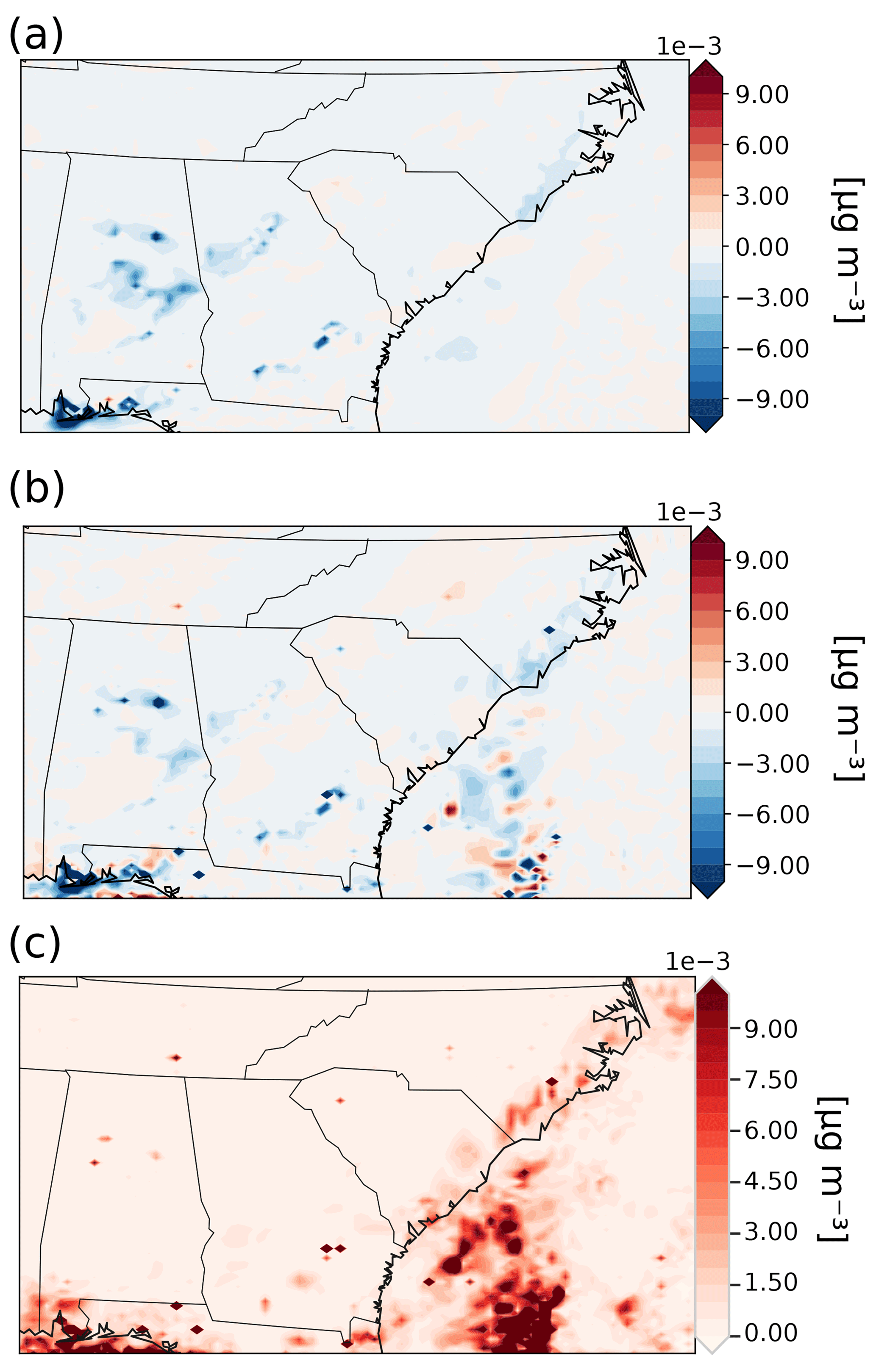
Figure 4 Comparisons of the sensitivities of aerosol-phase nitrate (ANO₃) with respect to SO₂ emission calculated by HYD and FDM on a map. (a) The HYD sensitivities. (b) The average of the FD sensitivities with three different perturbation size pairs (125 %, 75 %; 110 %, 90 %; 105 %, 95 %). (c) The range of FD sensitivities with three different perturbation size pairs (125 %, 75 %; 110 %, 90 %; 105 %, 95 %).

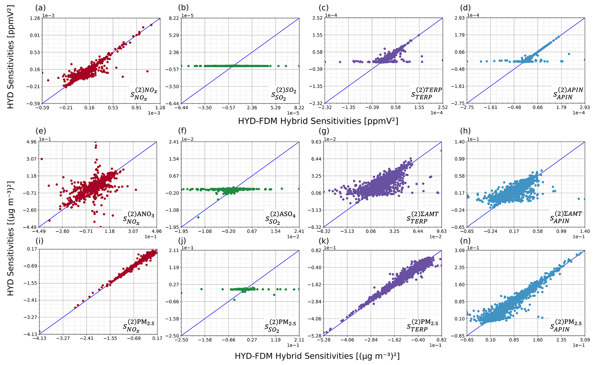
Figure 5 Comparisons of second-order sensitivities on the ground layer calculated by the hyperdual-step method (HYD sensitivities) and the hybrid HYD-FDM method (HYD-FDM sensitivities). The sensitivities are colour coded by the perturbed emissions (i.e. NO_x, SO₂, TERP, and APIN). Panels (a)–(d) show the gas-phase species sensitivities with respect to their emissions. APIN denotes α-pinene and TERP denotes all other monoterpene species. Panels (e)–(h) show examples of aerosol-phase products with respect to their precursors. ANO₃ denotes the total aerosol-phase nitrate products. ASO₄ denotes the total aerosol sulfate products. ΣAMT denotes the total aerosol photooxidation products from monoterpene. Panels (i)–(n) show the total PM_2.5 concentration with respect to gas-phase precursors. The sensitivities calculated are noted at the bottom-right corner of each panel with the notation pattern mentioned in Sect. 2.3.

Table 2 The slopes and R² values from the linear regression of the second-order sensitivities of ground-layer species concentrations to domain-wide perturbations by the hyperdual-step method compared to finite difference sensitivities. The gas-phase species sensitivities with respect to their emissions are on line three, where APIN denotes α-pinene and TERP denotes all other monoterpene species. Line four includes sensitivities of aerosol-phase products with respect to their precursors, where ANO₃ denotes the total aerosol-phase nitrate products, ASO₄ denotes the total aerosol sulfate products, and ΣAMT denotes the total aerosol photooxidation products from monoterpene. Line five includes the sensitivities of the total PM_2.5 concentration with respect to each gas-phase precursor. A visual comparison of the agreement for each relationship is shown in Fig. 5.

We also compared the second-order HYD sensitivities with those calculated from the hybrid HYD-FDM method (hybrid second-order sensitivities) described in Sect. 2.3 using one-to-one plots with identity lines for each panel (Fig. 4) along with the slope and R² values (Table 2). Additional slopes and R² values for second-order sensitivities can be found in Tables S1 and S2. Overall, the agreement between HYD and the hybrid second-order sensitivities is good except for those to SO₂ emissions. This result can be attributed to the numerical errors in the first-order sensitivities to SO₂, as illustrated in Figs. 2j and 3. Computing second-order sensitivities with the hybrid method, which includes FDM, is expected to add numerical noise. Except for $s_{{\mathrm{SO}}_{\mathrm{2}}}^{\left(\mathrm{2}\right){\mathrm{SO}}_{\mathrm{2}}}$, the hyperdual and hybrid second-order sensitivities of gas-phase species concentrations to emissions of the same species exhibit good agreement, with slopes and R² values ranging from 0.84 to 0.85 and 0.84 to 0.86, respectively (Table 2). The hybrid second-order sensitivities are sometimes large, while HYD predicts close-to-zero sensitivities. This result is especially evident in $s_{\mathrm{TERP}}^{\left(\mathrm{2}\right)\mathrm{TERP}}$ (Fig. 5c) and $s_{\mathrm{APIN}}^{\left(\mathrm{2}\right)\mathrm{APIN}}$ (Fig. 5d). This spread in the hybrid sensitivities likely originates from the FDM step, which is subject to numerical errors. Figure 5e–h show the HYD and HYD-FDM sensitivities of aerosol-phase product concentrations to the precursor emissions for this modelling period. Except for $s_{{\mathrm{SO}}_{\mathrm{2}}}^{{\mathrm{ASO}}_{\mathrm{4}}}$, the slope and R² values range from 0.61 to 0.82 and 0.38 to 0.71, respectively (Table 2). The degree of agreement for $s_{{\mathrm{NO}}_x}^{{\mathrm{ANO}}_{\mathrm{3}}}$ is slightly lower than those for $s_{\mathrm{TERP}}^{\mathrm{\Sigma }\mathrm{AMT}}$ and $s_{\mathrm{APIN}}^{\mathrm{\Sigma }\mathrm{AMT}}$, indicating more nonlinearity in the formation process from NO_x to aerosol nitrate. The second-order sensitivities of total PM_2.5 to different precursors demonstrate excellent agreement, with slope and R² values ranging from 0.95 to 0.99 and from 0.96 to 0.99 (Table 2), again excluding the one to SO₂. The second-order sensitivities of PM_2.5 to NO_x and α-pinene are primarily negative, while those to monoterpenes are positive. These findings have important implications for the formation process of PM_2.5 from monoterpenes and α-pinene, which will be discussed in detail in the next section.

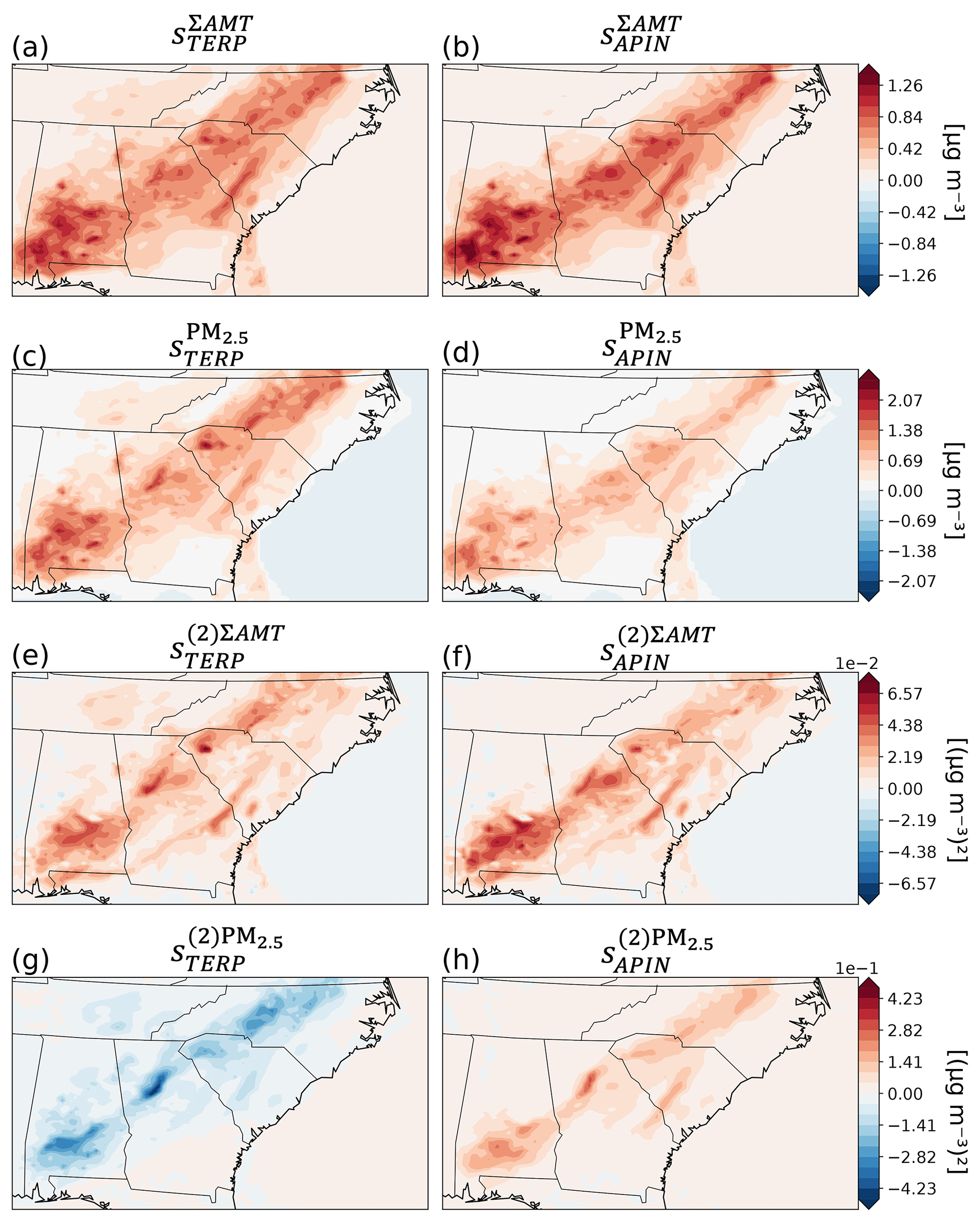
Figure 6 The first- and second-order sensitivities of total aerosol monoterpene photooxidation products (ΣAMT) and PM_2.5 with respect to monoterpene (TERP) and α-pinene (APIN) emissions plotted on a map. Panels (a)–(d) show the first-order sensitivities and (e)–(h) show the second-order sensitivities.

3.2 Sensitivities of biogenic aerosol formation in the Southeast US computed by CMAQ-hyd

In this section, the first- and second-order sensitivities of several biogenic aerosols to both anthropogenic and biogenic aerosol precursors in the Southeast US are explored. The importance of calculating second-order sensitivities is demonstrated through the spatial distributions of the first- and second-order sensitivities of total aerosol-phase monoterpene photooxidation product (ΣAMT) and PM_2.5 concentrations (Fig. 6). The first-order sensitivities (Fig. 6a–d) are predominantly positive, indicating that an increase in either TERP or APIN emissions will lead to an increase in ground-layer ΣAMT and PM_2.5 concentrations. While $s_{\mathrm{TERP}}^{\mathrm{\Sigma }\mathrm{AMT}}$ (Fig. 6a) and $s_{\mathrm{APIN}}^{\mathrm{\Sigma }\mathrm{AMT}}$ (Fig. 6b) have similar values, $s_{\mathrm{TERP}}^{{\mathrm{PM}}_{\mathrm{2.5}}}$ (Fig. 6c) is slightly larger than $s_{\mathrm{APIN}}^{{\mathrm{PM}}_{\mathrm{2.5}}}$ (Fig. 6d) due to the formation of other species, such as aerosol-phase monoterpene nitrate products (AMTNO₃). The second-order sensitivities (Fig. 6e–h) provide additional information about how ΣAMT and PM_2.5 concentrations respond to changes in APIN and TERP emissions. The $s_{\mathrm{TERP}}^{\left(\mathrm{2}\right)\mathrm{\Sigma }\mathrm{AMT}}$ (Fig. 6e) and $s_{\mathrm{APIN}}^{\left(\mathrm{2}\right)\mathrm{\Sigma }\mathrm{AMT}}$ (Fig. 6f) are generally positive, indicating that the response of the concentration of ΣAMT to monoterpene and α-pinene emissions is convex. An increase in either monoterpene or α-pinene emissions will lead to increases in $s_{\mathrm{TERP}}^{\mathrm{\Sigma }\mathrm{AMT}}$ and $s_{\mathrm{APIN}}^{\mathrm{\Sigma }\mathrm{AMT}}$. If we only consider first-order sensitivities, the effect of changes in TERP or APIN emissions on ΣAMT concentrations will be underestimated. On the other hand, $s_{\mathrm{TERP}}^{\left(\mathrm{2}\right){\mathrm{PM}}_{\mathrm{2.5}}}$ (Fig. 6g) is mostly negative, while $s_{\mathrm{APIN}}^{\left(\mathrm{2}\right){\mathrm{PM}}_{\mathrm{2.5}}}$ (Fig. 6h) is mostly positive. The distinct behaviour of the second-order sensitivities of PM_2.5 concentration to either TERP or APIN emissions exemplifies the importance of considering second-order sensitivities for these nonlinear formation processes. Only considering the first-order sensitivities often leads to the overestimation or underestimation of the effects. The accurate second-order sensitivity information can help researchers understand the relationships of concentration to emissions more thoroughly and develop emission control strategies for specific aerosol precursor emissions.

We used the formation of aerosol monoterpene nitrate, AMTNO₃, as an example of the importance of computing the cross-sensitivity, especially for complex anthropogenic–biogenic aerosol formation processes. The formation of AMTNO₃ is influenced primarily by two precursors: NO_x and monoterpenes. NO_x is primarily emitted anthropogenically, while monoterpenes primarily originate from biogenic sources. The first- and second-order sensitivities of AMTNO₃ to NO_x or TERP can help researchers and environmental decision makers estimate the nonlinear effects of emissions changes on concentrations of secondary pollutants. The cross-sensitivity of AMTNO₃ with respect to both NO_x and TERP emissions, $s_{{\mathrm{NO}}_x,\mathrm{TERP}}^{\left(\mathrm{2}\right){\mathrm{AMTNO}}_{\mathrm{3}}}$, is a valuable tool for answering complex research questions. For instance, researchers can use $s_{{\mathrm{NO}}_x,\mathrm{TERP}}^{\left(\mathrm{2}\right){\mathrm{AMTNO}}_{\mathrm{3}}}$ to predict how an increase in monoterpene emissions would affect the first-order sensitivities of AMTNO₃ to NO_x. Since biogenic emissions of monoterpenes are temperature dependent, understanding how anthropogenic emissions of NO_x will affect AMTNO₃ formation with changing terpene emissions in future scenarios is crucial for designing effective air pollution control strategies. Computing the cross-sensitivity is especially challenging with traditional methods since determining the proper perturbation for two species using FDM is even harder than calculating second-order sensitivities with FDM. The distinct values of $s_{{\mathrm{NO}}_x}^{\left(\mathrm{2}\right){\mathrm{AMTNO}}_{\mathrm{3}}}$, $s_{\mathrm{TERP}}^{\left(\mathrm{2}\right){\mathrm{AMTNO}}_{\mathrm{3}}}$, and $s_{{\mathrm{NO}}_x,\mathrm{TERP}}^{\left(\mathrm{2}\right){\mathrm{AMTNO}}_{\mathrm{3}}}$ demonstrate the value of the HYD method (Fig. 7). The spatial distributions of $s_{{\mathrm{NO}}_x}^{{\mathrm{AMTNO}}_{\mathrm{3}}}$ and $s_{\mathrm{TERP}}^{{\mathrm{AMTNO}}_{\mathrm{3}}}$ are included in Fig. S1 in the Supplement. Overall, the second-order sensitivities are negative over land in the Southeast US. $s_{{\mathrm{NO}}_x}^{\left(\mathrm{2}\right){\mathrm{AMTNO}}_{\mathrm{3}}}$ is generally smaller than $s_{\mathrm{TERP}}^{\left(\mathrm{2}\right){\mathrm{AMTNO}}_{\mathrm{3}}}$, indicating that the relationship between AMTNO₃ and TERP emissions is more nonlinear than that between AMTNO₃ and NO_x. The cross-sensitivities $s_{{\mathrm{NO}}_x,\mathrm{TERP}}^{\left(\mathrm{2}\right){\mathrm{AMTNO}}_{\mathrm{3}}}$ are mostly positive over the Southeast US. Based on the cross-sensitivity results, we can conclude that an increase in TERP emission will make the first-order sensitivity of AMTNO₃ to NO_x larger. A warmer climate in the future would likely increase the impact of anthropogenic NO_x on the AMTNO₃ concentration in the atmosphere. This kind of information is invaluable for researchers and environmental decision makers aiming to evaluate complex secondary organic aerosol formation with multiple anthropogenic and biogenic precursors.

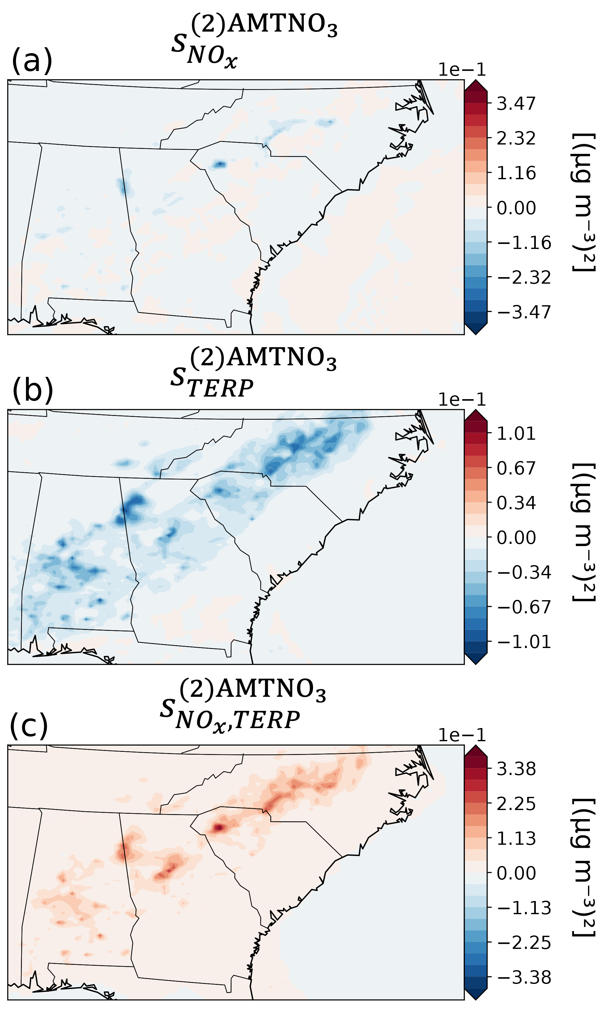
Figure 7 The second-order sensitivities and cross-sensitivities of aerosol-phase monoterpene nitrate products (AMTNO₃) with respect to NO_x and monoterpene (TERP) emissions plotted on a map. (a) Second-order sensitivities of AMTNO₃ with respect to NO_x. (b) Second-order sensitivities of AMTNO₃ with respect to TERP. (c) Cross-sensitivities of AMTNO₃ with respect to NO_x and TERP.

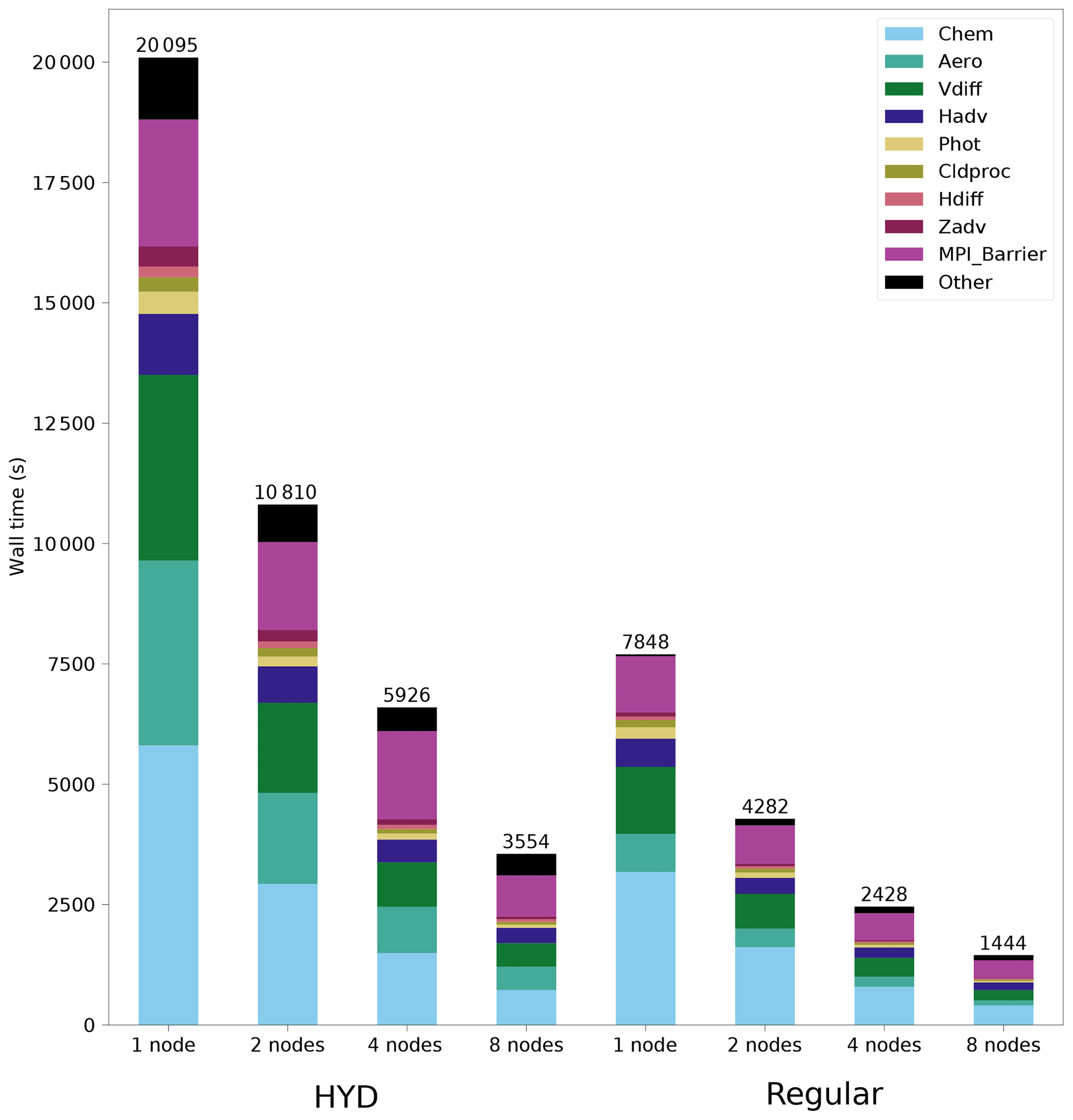
Figure 8 Computational costs of CMAQ-hyd and standard CMAQ, and the computational costs of various modules in them. CMAQ-hyd and standard CMAQ simulations using different numbers of nodes (one, two, four, and eight) are shown on the x axis. The wall time is shown on the y axis.

3.3 Computational cost of CMAQ-hyd

The practical application of any sensitivity analysis in CTMs depends heavily upon its computational cost. Previous works using operator overloading approaches resulted in high computational costs due to additional mathematical operations, making this approach computationally unfavourable compared to other existing methods. For instance, the implementation of CVM in GEOS-CHEM results in a 4.5-fold increase in computational overhead when compared to the standard model (Constantin and Barrett, 2014). To evaluate the computational efficiency of CMAQ-hyd, we compared it with a standard CMAQ model using different computational resources in a supercomputing cluster. The total wall times needed when different numbers of computational nodes are used for an identical run of the original CMAQ model and CMAQ-hyd are displayed in Fig. 8. The CMAQ-hyd and standard CMAQ runs were performed with one, two, four, and eight nodes of the supercomputing cluster. The configuration of computing resources is detailed in Sect. S4 of the Supplement. Profiling of the model was completed at the level of the scientific modules, special subroutines, or other important components of CMAQ. The scientific processes are Chem (gas-phase chemistry), Aero (aerosol dynamics and thermodynamics), Vdiff (vertical diffusion), Hadv (horizontal advection), Phot (photolysis), Cldproc (cloud processes), Hdiff (horizontal diffusion), and Zadv (vertical advection). MPI_Barrier is a special subroutine used for synchronizing processes among parallel processors after vertical diffusion and before the other three transport processes. Other processes necessary for CMAQ, including the I/O processes, are included in the “Other” category. Details about the high-performance computing cluster used can be found in the Supplement.

With the same computing resources, the total computation time of CMAQ-hyd is approximately 2.5 (2.44–2.56) times longer. Despite the additional computational burden, CMAQ-hyd remains computationally competitive with the traditional FDM when calculating derivatives. One run of CMAQ-hyd generates the same amount of first- and second-order sensitivity information as at least three runs of standard CMAQ. The relatively low computational cost of CMAQ-hyd compared to the previous operator overloading approach may be due to the selective modification of the source code. In contrast to GEOS-CHEM CVM (Constantin and Barrett, 2014), only the parts of the model that involve calculating the main species concentration array use hyperdual calculations.

The computational times of scientific modules in CMAQ-hyd generally scale well with increases in computational resources, similar to standard CMAQ. Chem, Aero, and Vdiff are the most computationally expensive modules in both CMAQ and CMAQ-hyd. The relative computational cost of Aero is higher in CMAQ-hyd than in standard CMAQ. The ratio of the computational time of Chem to that of Aero is 1.53 (1.49–1.56) for the CMAQ-hyd runs and 3.98 (3.85–4.19) for the standard CMAQ runs (Fig. 8). Future work can potentially reduce the computational cost by ignoring sensitivity propagations during the iterative root-finding process in select subroutines, since only the output concentrations from these subroutines are used in the later part of the model. This is also a significant advantage of any operator-overloading-based approach (Fike and Alonso, 2011). The computational time of each module is detailed in Table S3 in the Supplement, and the full relative percentage of the computational time of each module in eight runs is shown in Fig. S2 in the Supplement.

The MPI_Barrier function also scales well with an increasing number of processors. To a certain point, subdividing the domain further reduces the variability of the time required for scientific processes to be completed across different nodes, resulting in a reduction in the amount of time the program spends waiting for all processes to be synchronized. One important thing to note here is that the scaling of MPI_Barrier is dependent on the ratio of the number of nodes to the number of grid cells. A demonstration of the subdivision of the modelling domain by processors is shown in Fig. S3 in the Supplement.

The I/O process for newly added first- and second-order sensitivity output files increases the computational cost; however, the I/O of species concentration files has a much lower computational cost than other modules in CMAQ for this specific scenario. The I/O processes of CMAQ-hyd and CMAQ take 193 (181–206) s and 52 (47–56) s, respectively. The I/O process of CMAQ-hyd takes approximately 3.7 times longer on average than that of standard CMAQ. The overall memory overhead of CMAQ-hyd is approximately 25 GB for this simulation. A parallel input/output (I/O) approach may be applied to reduce the possibility of potential memory overflow in processor 0 (Wong et al., 2015).

4 Conclusion

We have demonstrated the implementation of the hyperdual-step method in CMAQ version 5.3.2 to formulate CMAQ-hyd. This novel model retains the majority of the CMAQ code with slight modifications in the declarations of selected variables and the addition of sensitivity computation modules. The novel model can be applied to compute exact first-order sensitivities, second-order sensitivities, and cross-sensitivities of pollutant concentrations to precursor emissions efficiently and accurately with a single model run. Compared with traditional sensitivity analysis methods, CMAQ-hyd is computationally competitive with conventional methods and easier to maintain than other existing advanced methods (DDM and adjoint). The development process of CMAQ-hyd is also more straightforward than that of other advanced methods, since all that is needed is to change the type of newly declared variables to hyperdual.

We developed and validated the hyperdual-step module “HDMod”, which is limited to analytically verifiable mathematical operations of hyperdual numbers. This module can also be applied to other numerical models where first- and second-order sensitivities are of interest. We further evaluated the development of CMAQ-hyd against the FDM and the FDM-HYD hybrid method to ensure the correctness of the implementation. During the evaluation process, CMAQ-hyd demonstrated the ability to compute sensitivities free from truncation and subtractive cancellation errors, unlike those calculated by the FDM. HDMod can potentially be applied to other numerical models written in Fortran to produce first- and second-order sensitivities.

The computation of second-order sensitivities is crucial for researchers and environmental decision makers who need to decide the priority and extent of controls on specific types of emissions to reduce atmospheric pollutant concentrations. For instance, the second-order sensitivity of PM_2.5 concentration to monoterpenes and α-pinene provided additional information about the relationships of emissions to concentrations in CMAQ. With the additional second-order sensitivity information, the curvature of the concentration responses to emissions changes improves the estimate of how a specific pollutant concentration would respond to changes in emissions. The simplicity of computing cross-sensitivities with CMAQ-hyd is another advantage of this augmented model. Cross-sensitivities are especially useful in nonlinear processes with two precursors. Knowledge of the synergistic effect of anthropogenic and biogenic emissions on aerosol concentrations (e.g. NO_x and monoterpene on AMTNO₃) is essential for researchers to predict the dynamics between two potential pollutants and for environmental decision makers to propose policy implementations under different climate scenarios in the future.

Although CMAQ-hyd remains computationally competitive with the traditional finite-difference method, it is still computationally intensive and has a memory overhead. We plan to implement optimizations for iterative processes in CMAQ and to apply the parallel I/O approach to reduce the memory overhead on the compute node where all the information is gathered. The implementation of checkpointing of sensitivities after specific subroutines is also a potential advantage of CMAQ-hyd and will provide valuable information on how each module or even each line of the model affects the sensitivities, akin to a process analysis approach. This checkpointing feature cannot be easily implemented with other methods such as FDM, DDM, and the adjoint method.

In conclusion, we have developed and evaluated CMAQ-hyd, a novel augmented model to compute first-order sensitivities, second-order sensitivities, and cross-sensitivities free from subtractive cancellation and truncation errors in CMAQ. Our successful implementation also provides an example of the hyperdual-step method that may be applicable for other CTMs where sensitivities are helpful.