New routine NLTE15µmCool-E v1.0 for calculating the non-local thermodynamic equilibrium (non-LTE) CO₂ 15 µm cooling in general circulation models (GCMs) of Earth's atmosphere

We present a new routine for calculating the non-local thermodynamic equilibrium (non-LTE) 15 µm CO₂ cooling–heating of mesosphere and lower thermosphere in general circulation models. It uses the optimized models of the non-LTE in CO₂ for day and night conditions and delivers cooling–heating with an error not exceeding 1 K d⁻¹ even for strong temperature disturbances. The routine uses the accelerated lambda iteration and opacity distribution function techniques for the exact solution of the non-LTE problem and is about 1000 times faster than the standard matrix and line-by-line solution. It has an interface for feedbacks from the model and is ready for implementation. It may use any quenching rate coefficient of the CO₂(ν₂)+O(³P) reaction, handles large variations in O(³P), and allows the user to vary the number of vibrational levels and bands to find a balance between the calculation speed and accuracy. The suggested routine can handle the broad variation in CO₂ both below and above the current volume mixing ratio, up to 4000 ppmv. This allows the use of this routine for modeling Earth's ancient atmospheres and the climate changes caused by increasing CO₂.

1 Introduction

The infrared radiative cooling of atmosphere is an important component of its energy budget. It requires special techniques for reliable estimation. For the local thermodynamic equilibrium (LTE), when the molecular emissions of the atmospheric unit volume are described by the Planck function for local temperature, this estimation is confined to the solution of the radiative transfer equation in broad spectral regions occupied by molecular bands. In the middle and upper atmosphere, the breakdown of LTE (non-LTE) requires finding the sources of the non-equilibrium molecular emissions, which are obtained by the solution of the non-LTE problem. This makes the non-LTE cooling calculation significantly more time-consuming. Today, common opinion is that it is impossible to use exact methods for calculating the radiative cooling in general circulation models (GCMs); see, for instance, López-Puertas et al. (2024), who promote this point of view. Various parameterizations have been developed for quickly calculating this cooling in GCMs; see Fomichev et al. (1998), Fomichev (2009), and Feofilov and Kutepov (2012) for reviews of works on parameterizing the non-LTE cooling of Earth’s middle atmosphere in the 15 µm CO₂, 9.6 µm O₃ and rotational H₂O bands. These algorithms, however, lack the accuracy needed for current GCMs.

Infrared emission in the 15 µm CO₂ band is the main cooling mechanism of middle and upper atmospheres of Earth, Venus and Mars (e.g., Goody and Yung, 1995; Sharma and Wintersteiner, 1990; Pollock et al., 1993; Bougher et al., 1994; López-Puertas and Taylor, 2001; Feofilov and Kutepov, 2012). On Earth, the magnitude of the mesosphere and lower-thermosphere (MLT) cooling affects both the mesospheric temperature and the mesospheric height: the stronger the cooling, the colder and higher the mesopause (Bougher et al., 1994).

The goal of this work is to present a new routine for calculating the non-LTE 15 µm CO₂ cooling of Earth’s MLT, which utilizes exact radiative transfer and non-LTE problem solution techniques and is fast enough to be applied in GCMs. The new routine can handle the broad variation in CO₂ both below and above the current volume mixing ratio, up to 4000 ppmv. This allows the use of this routine for modeling Earth’s ancient atmospheres and the climate changes caused by increasing CO₂.

The routine we present is the optimized version of the research ALI-ARMS (Accelerated Lambda Iteration for Atmospheric Radiation and Molecular Spectra) model and code (Kutepov et al., 1998; Feofilov and Kutepov, 2012). In this code, atmospheric cooling is the by-product of the non-LTE problem solution. For nearly 20 years, the earlier version of this routine has been successfully applied (Hartogh et al., 2005; Medvedev et al., 2015) in the GCM of Martian atmosphere.

In this paper, we demonstrate the performance of the routine for calculation of the 15 µm CO₂ cooling of Earth’s MLT. However, generally this is a universal code, which potentially may be applied to modeling the non-LTE cooling in any molecular band or bands of several molecules in any planetary atmosphere. We successfully tested it calculating the non-LTE cooling of Earth's MLT in the 6.3 µm H₂O band (Feofilov et al., 2009) and 9.6 and 4.7 µm O₃ bands (Manuilova et al., 1998) as well as the cooling of Titan atmosphere in the 6.7 and 3.3 µm CH₄ bands (Kutepov et al., 2013a; Feofilov et al., 2016). This potentially allows the application of this algorithm for calculating the radiative cooling in GCMs of various atmospheres; among them, the atmospheres of water reach exoplanets (e.g., Valencia et al., 2007; Acuña et al., 2021) and gas giants.

In the next section, we outline techniques currently applied in GCMs for calculating the non-LTE CO₂ 15 µm cooling. In Sect. 3, we briefly discuss the method and techniques applied for calculating this cooling in our new routine. In Sect. 4, we present the model of non-LTE in CO₂ used in the routine and the routine computational performance. Section 5 discusses the accuracy of the new routine. The Conclusions (Sect. 6) summarize the results of our study. Appendix A contains technical details of the code and recommendations for its implementation and usage in GCMs.

2 The non-LTE radiative cooling of atmosphere and its calculations in general circulation models

The energy loss of the atmospheric unit volume due to infrared radiation is calculated as the radiative flux divergence taken with the opposite sign:

$$\begin{array}{}\text{(1)}& \mathit{h}=-{\displaystyle \frac{\mathrm{1}}{\mathrm{4}\mathit{\pi }}}\int \mathrm{d}\mathit{\omega }\int \mathrm{d}\mathit{\nu }{\displaystyle \frac{\mathrm{d}{I}_{\mathit{\nu }\mathit{\omega }}}{\mathrm{d}s}},\end{array}$$

where I_μν is the intensity of radiation at the frequency ν along the ray ω.

With the local thermodynamic equilibrium (LTE), the discretization of the integral radiative transfer equation (RTE) (e.g., Goody, 1964; Goody and Yung, 1995) leads to a simple linear algebra operation for calculating the LTE 15 µm band cooling:

$$\begin{array}{}\text{(2)}& \mathit{h}=\mathbf{W}\times \mathit{B},\end{array}$$

where h is the vector of cooling in N_D grid points; B is the vector of the Planck function for a local T; and W is an N_D×N_D matrix, which accounts for radiative transfer in a number of 15 µm CO₂ bands contributing to the total cooling.

Extension of GCMs to the mesosphere and thermosphere required accounting for the non-LTE for calculating the CO₂ 15 µm cooling. The standard way of solving the non-LTE problem (e.g., Curtis and Goody, 1956; Goody, 1964; Goody and Yung, 1995) requires inverting the $(N_{\mathrm{L}}\times N_{\mathrm{D}})\times (N_{\mathrm{L}}\times N_{\mathrm{D}})$ matrix, where N_L is the number of CO₂ vibrational levels included in the model. Equation (2) in this case remains unchanged; however, the matrix W is rebuilt to account for differences between the Planck function and the non-LTE source functions in each band resulting from the non-LTE problem solution. This makes the calculation of the non-LTE cooling dramatically costlier (see Sect. 3 for more details).

Fomichev et al. (1998) and Fomichev (2009) (see references therein) discussed in detail various routines that had been suggested in previous studies for calculating the 15 µm cooling in GCMs while accounting for the non-LTE. The direct matrix solution of the simplified non-LTE problem in CO₂ (often with an approximate radiative transfer treatment) or using pre-calculated W matrices for a limited number of atmospheric situations for further interpolation of its elements helped to reduce computational time at the expense of calculation accuracy.

A new way of calculating the non-LTE 15 µm CO₂ cooling in GCMs was suggested by Kutepov (1978). Relying on results of Kutepov and Shved (1978), who showed that the fundamental 15 µm CO₂ band 01101→00001 (see below, Fig. 1) of the main CO₂ isotope dominates the cooling above about 85 km, Kutepov (1978) derived the recursive expression for h coming from the analytical solution of the first-order differential equation for the non-LTE cooling h in the fundamental band. This expression directly accounted for the CO₂(ν₂)+O(³P) quenching rate coefficient k and the O(³P) density. It was derived using the “second-order escape probability” approach (Frisch and Frisch, 1975; Frisch, 2022) for the approximate solution of the Wiener–Hopf-type integral radiative transfer equation in the semi-infinite atmosphere. The algorithm of Kutepov (1978) – see its refined version by Kutepov and Fomichev (1993) – calculates h upward in the non-LTE layers using the LTE h or the non-LTE h obtained using other techniques as a lower boundary condition. Fomichev et al. (1993) linked this algorithm to the matrix routine for calculating h in the LTE layers developed by Akmaev and Shved (1982). Later Fomichev et al. (1998) modified the routine of Fomichev et al. (1993) by adding the interpolation of the W matrices for the CO₂ within 150–720 ppmv using tables of pre-calculated elements, and they described in detail the structure of the revised matrix W. These authors also extended the routine altitude range to layers above 110 km. Cooling in this region is calculated from the simple balance equation for the first excited vibrational level of the main CO₂ isotope while accounting for absorption of the radiative flux from below, cooling to space and collisional quenching. For smooth temperature profiles, Fomichev et al. (1998) reported maximal cooling calculation errors of less than 2 and up to 5 K d⁻¹, for 360 and 720 ppmv CO₂, respectively. In this paper we will call this routine F98.

Basic features of F98, namely (a) a broad altitude range covered, (b) straightforward accounting for the non-LTE, and (c) high computational efficiency, attracted many users. For more than 2 decades, the F98 routine has been the most widely used algorithm for calculating the 15 µm CO₂ cooling in GCMs of mesosphere and thermosphere; see, for instance, Eckermann (2023) for its latest application. However, as we show below, the F98 errors are large for non-smooth temperature profiles reaching 20–25 K d⁻¹ in the mesopause region. On the other hand, even very minor variation in the CO₂ cooling may have significant impact on the GCM results in MLT. Kutepov et al. (2013b) showed (their Fig. 18.2) that variation in the CO₂ cooling of ∼ 1–3 K d⁻¹ in the Leibniz Institute Middle Atmosphere (LIMA) model (Berger, 2008) in the mesopause region caused significant warming of up to 5–6 K (about 105 km) and cooling of up to −10 K (below 105 km) at latitudes between 90° S and 40° N for July 2005. This and other tests lead to the conclusion (Uwe Berger, personal communication, 2010) that the accuracy of cooling–heating rate calculations in GCMs “should not exceed 1 K d⁻¹ for any temperature distribution”.

Fortunately, this accuracy requirement overlapped in time with the dramatic progress in the non-LTE radiative transfer calculations. This allowed the development of a new routine, NLTE15µmCool-E (hereafter KF23 for brevity within this paper), for calculating the non-LTE 15 µm CO₂ cooling in GCMs of Earth's atmosphere; the routine exploits new exact algorithms for solving the non-LTE problem and, therefore, fits enhanced accuracy requirements. At the same time, it is fast enough to be used in GCMs.

KF23 is the optimized version of our basic ALI-ARMS model and code (Kutepov et al., 1998; Feofilov and Kutepov, 2012), which utilizes two advanced techniques: (1) the ALI technique for the solution of the non-LTE problem and (2) the opacity distribution function (ODF) technique for optimizing the radiative transfer calculations. In this section, we outline these techniques and the current status and latest applications of ALI-ARMS code.

3 Method and techniques applied in a new routine for calculating the non-LTE cooling

3.1 Solution of the non-LTE problem

The non-LTE problem has two primary constituents: (1) the statistical equilibrium equations (SEEs), which express the equality of the total population and de-population rates for each molecular level, and (2) the radiative transfer equation (RTE), which relates the radiation field to the populations of levels, at all altitudes in the atmosphere (Hubeny and Mihalas, 2015). Hence, the system of equations for the level populations is non-local (and non-linear). The most obvious way of dealing with this situation is to iterate between the SEEs and RTE. This process, traditionally called “lambda iteration” (LI), has been investigated in the astronomical context since the 1920s (Unsöld, 1938). It inverts N_D matrices N_L×N_L at each iteration step. This simple approach has been applied in Earth's and planetary atmosphere radiative transfer; see, for instance Appleby (1990) and Wintersteiner et al. (1992). If the optical depths are large (as is the case for the CO₂ 15 µm band), the algorithm converges slowly. Kutepov et al. (1998) studied several LI schemes and showed that for the CO₂ non-LTE problem, the number of iterations I_LI for these algorithms may reach ∼ 200 for even moderate convergence criterion $\mathrm{1}\times {\mathrm{10}}^{-\mathrm{3}}$. This slow convergence is caused by the photons trapped in the cores of the most optically thick lines and by the strong non-linearity of SEEs related to quasi-resonant exchange of vibrational energy by the molecular collisions.

An alternative way of dealing with the non-LTE is a joint treatment of SEEs and RTE, when RTE is discretized with respect to the optical depth or altitude grid to get a matrix representation of radiative terms in SEEs. This approach, known in the atmospheric science as the Curtis matrix (CM) technique (e.g., Goody, 1964; Goody and Yung, 1995; López-Puertas and Taylor, 2001), leads to a matrix of dimensions $(N_{\mathrm{L}}\times N_{\mathrm{D}})\times (N_{\mathrm{L}}\times N_{\mathrm{D}})$. In stellar atmosphere studies, the generalized version of this technique is known as the Rybicki method (Mihalas, 1978). The time required for the solution of the non-LTE problem using the CM technique is controlled by the number of operations for matrix inversion. The advantage of the classic matrix method lies in the simultaneous determination of all populations at all altitudes instead of the sequential evaluation of populations step by step at each altitude using the radiative field from the previous iteration. Therefore, “matrix iteration” usually converges better than lambda iterations. However, the convergence of both algorithms depends strongly on how the local non-linearity is treated; see the next section. To construct an adequate model, one must account for a large number of excited levels of various molecular species plus use a detailed model of atmospheric stratification. As a result both N_L and N_D can become very large. The dimensions of primary matrices are reduced by introducing various assumptions (for instance, the LTE assumption for rotational sublevels as well as, for example, LTE in the groups of vibrational levels closely spaced in energy; see also the discussion of GRANADA – Generic RAdiative traNsfer AnD non-LTE population Algorithm – code in Sect. 3.4). Nevertheless, usually the time to solve the non-LTE problem using the CM method significantly exceeds the time needed when an LI algorithm is applied to the same problem (see Sect. 5 for more details).

In the 1990s, stellar astrophysicists developed a family of powerful techniques that utilize lambda iteration with an approximate (or accelerated) lambda operator (see Rybicki and Hummer, 1991; Rybicki and Hummer, 1992; and references therein). In these so-called ALI techniques (for accelerated lambda iteration), the integral lambda operator, which links the radiation intensity at a given point with the source function at all points, is approximated by a local (or nearly local) operator. With a local operator, the largest matrices again, as in the LI case, have dimensions N_L×N_L. However, in this case, the convergence is rapid, since most of the transfer in cores of the lines (described by the local part of lambda operators) cancels out analytically and only the difference between exact and approximate radiative terms in the SEEs is treated iteratively. Kutepov et al. (1998) shoved that for the CO₂ non-LTE problem I_ALI≪I_LI (see Sect. 5 for more details).

3.2 Treating the strong local non-linearity caused by intensive VV exchange

Strong local non-linearity of the non-LTE radiative transfer problem in molecular bands caused by intensive near-resonant exchange of vibrational energy between molecules was studied by Kutepov et al. (1998). They showed that this non-linearity causes a dramatic deceleration of the convergence. Various schemes of additional “internal” iterations (without recalculating radiative excitation rates) aimed at adjusting populations of levels coupled by strong inter- and intramolecular vibrational–vibrational (VV) exchange did not bring any help. To accelerate the convergence, Kutepov et al. (1998) suggested “decoupling”, which utilizes the Avrett (1966) approach of treating the “source function equality in the line multiples”. The SEE terms, which describe the VV coupling, depend on the products $n_v{n}_{v^{\prime }}$, where n_v is the population of vibrational level v of one molecular species, whereas $n_{v^{\prime }}$ is the population of level v^′ of the same or another molecular species. In the iteration process, one needs to present these terms as $n_v{n}_{v^{\prime }}^{†}$, where † denotes the population of the level with the lower degree of excitation, which is taken from the previous iteration. Kutepov et al. (1998) showed that this stops “the propagation of errors” by iterations and guarantees the fastest convergence. This decoupling requires only slight modification of matrices to be inverted (without additional linearization of the non-LTE problem and, therefore, additional programming efforts). It provides, however, the same acceleration of convergence as the application of the Newton–Raphson method for the solution of a system of non-linear equations (Gusev and Kutepov, 2003).

3.3 The radiative transfer in the molecular bands

With line-by-line (LBL) calculations, a very large number of frequency points to be accounted for significantly decelerate calculations of the 15 µm CO₂ radiative fluxes. In LTE the reduction in frequency points is usually achieved by utilizing the so-called CKD (for correlated k distribution) method, which is based on grouping the gaseous spectral transmittances in accordance with the absorption coefficient k. The accuracy of this approach is better than 1 %; see, for instance, Fu and Liou (1992). However, the k correlation is not applicable under the non-LTE conditions because the vibrational level populations involved in the k distributions are unknown and depend themselves on the solution of the radiative transfer equation.

To overcome this problem, stellar astrophysicists developed the ODF technique. In this approach, they treat the non-LTE radiative transfer in “super-lines” associated with multiplets of very large line numbers (e.g., Hubeny and Lanz, 1995; Hubeny and Mihalas, 2015). They re-sample the normalized absorption and emission cross sections of super-lines, consisting of hundreds or thousands of lines, to yield a monotonic function of frequency that can be represented by relatively small numbers of frequency points. Though the idea is like k correlation, these normalized absorption and emission profiles do not depend on the total populations of upper and lower “super-levels” but only on the relative population of sublevels that are closely spaced in energy within each super-level, which are supposed to be in LTE.

Feofilov and Kutepov (2012) described the adaptation of the ODF technique to the solution of the CO₂ non-LTE problem. They treated each CO₂ band branch as a super-line. Therefore, each CO₂ band was presented by only three lines for perpendicular bands and two lines for parallel bands. This way of treating the radiative transfer in the molecular band is about 50–100 times faster than the classic LBL approach. Whereas in the LBL approach the radiation transfer equation is solved for each of N_F frequency grid points within each rotational–vibrational line, in the ODF techniques the same number of frequency grid points as applied only to each super-line. Thus, the acceleration factor is approximately equal to the number of rotational–vibrational lines in the branch. As Feofilov and Kutepov (2012) show, the ODF approach introduces very small errors into the 15 µm cooling. For current CO₂ density (400 ppm in the lower atmosphere), these errors do not exceed 0.3 K d⁻¹ in a broad range of temperature variations; see Fig. 18 of Feofilov and Kutepov (2012). They increase roughly linearly with the CO₂ increase.

3.4 From matrix and LI to ALI techniques

Since the 1960s, the Curtis matrix algorithms, with the rare exceptions for LI mentioned above in Sect. 3.1, have been dominating the solution of the non-LTE problems in Earth's and planetary atmospheres, including the studies of the 15 µm CO₂ cooling (see, for instance, the work by Zhu, 1990, who developed Curtis matrix parameterization of CO₂ cooling of MLT, which was very advanced for that time). Numerous non-LTE studies of the research group from the Institute of Astrophysics of Andalusia, Granada, applied the GRANADA (Generic RAdiative traNsfer AnD non-LTE population Algorithm) code described by Funke et al. (2012). The core of it is a standard CM algorithm, which the authors in this and their earlier publications prefer to called MCM (for modified Curtis matrix). The cited paper discusses various ways of splitting large matrices into blocks, solving the non-LTE problem for selected sub-sets of levels and iterating to get the solution for all vibrational levels. In stellar astrophysics (Mihalas, 1978), this approach is known as the “generalized equivalent two-level approach for multi-level problems”. For many years it has had no use because of convergence problems. The GRANADA code also includes LI but not the ALI technique, although the transformation of LI into ALI requires a minimum of programming efforts but speeds up the convergence for optically thick problems at least 10-fold (e.g., Rybicki and Hummer, 1991; Kutepov et al., 1998). Additionally, Funke et al. (2012) neither compared the computational performance of MCM and LI algorithms nor described the handling of a strong local non-linearity caused by VV coupling.

3.5 The ALI-ARMS code

Kutepov et al. (1991, 1997) successfully applied the ALI technique to study the non-LTE emissions of molecular gases in planetary atmospheres (the 4.3 µm CO₂ band in the Martian atmosphere and the 4.7 µm CO band in Earth's atmosphere, respectively). Kutepov et al. (1998) and Gusev and Kutepov (2003) described in detail the adaptation of the ALI code developed by Rybicki and Hummer (1991) for stellar atmospheres to the solution of the non-LTE problem for molecular bands of planetary atmospheres. They studied the performance of the new ALI-ARMS code and demonstrated computational superiority of ALI-ARMS compared to various LI and CM/MCM techniques. The ALI-ARMS code and its applications were described by Feofilov and Kutepov (2012). Later it was applied to study the rotational non-LTE in the CO₂ 4.3 µm band in Martian atmosphere, observed by the Planetary Fourier Spectrometer (PFS) in the Mars Express mission (Kutepov et al., 2017, and references therein); to study self-consistent two-channel CO₂ and temperature retrievals from the limb radiance measured by the SABER (Sounding of the Atmosphere using Broadband Emission Radiometry) instrument on board the Thermosphere Ionosphere Mesosphere Energetics and Dynamics (TIMED) Mission (Rezac et al., 2015); and to explain the SABER nighttime CO₂ 4.3 µm limb emission enhancement caused by a recently discovered new channel of energy transfer from OH(ν) to CO₂ and to simultaneous retrievals of O(³P) and total OH densities in the nighttime MLT (Panka et al., 2017, 2018, 2020). Earlier, the ALI-ARMS code was used (Kutepov et al., 2006) to pinpoint an important missing process of strong VV coupling between the isotopes in the CO₂ non-LTE model of the SABER operational algorithm and to model the H₂O 6.3 µm emission and the H₂O density retrievals in MLT from the SABER 6.3 µm limb radiances (Feofilov et al., 2009). As we show below in Sects. 4 and 5, the ALI-ARMS code also provides an efficient way of calculating the 15 µm CO₂ cooling–heating in the GCMs.

4 New routine for the CO₂ cooling calculations

4.1 The CO₂ non-LTE day- and nighttime models

To optimize the cooling calculations, we used as a reference our working line-by-line non-LTE model in CO₂, which comprises 60 vibration levels of five CO₂ isotopic species and two levels of N₂, O₂ and O(³P). In Fig. 1, we show the lower levels of this model (up to 5000 cm⁻¹). The set of collisional rate coefficients for the vibrational–translational (VT) and VV exchange that we apply is described by Shved et al. (1998) and is similar to rates used by López-Puertas and Taylor (2001). However, it relies on different scaling rules based on first-order perturbation theory. Compared to our extended line-by-line model (Feofilov and Kutepov, 2012), which includes a total of about 350 vibrational levels of seven CO₂ isotopes and over 200 000 rotational–vibrational lines, the CO₂ cooling of the 60-level model differs by less than 0.05 and 0.5 K d⁻¹ for the CO₂ mixing ratios of 400 and 4000 ppmv, respectively, for both daytime and nighttime conditions and for any temperature profile.

In the next steps, we gradually reduced the number of levels and bands in the model to optimize the calculations, keeping the cooling rate errors smaller than 1 K d⁻¹ compared to the reference model.

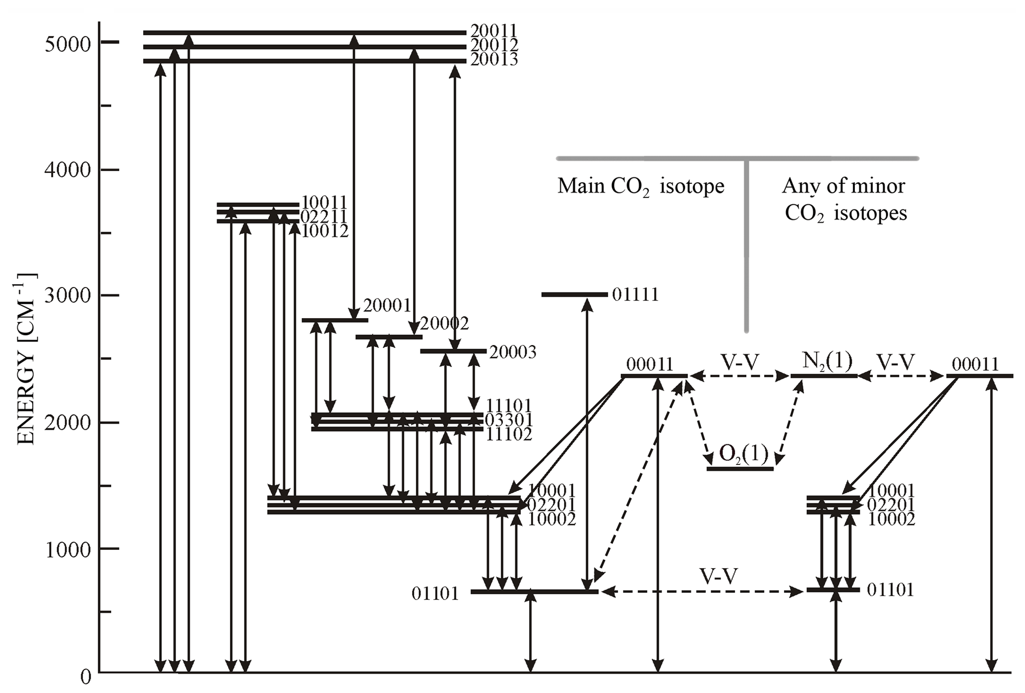
Figure 1 CO₂ vibrational level diagram (Feofilov and Kutepov, 2012). We use the HITRAN (high-resolution transmission molecular absorption database) notation for vibrational levels. The main optical transitions are shown by solid lines with arrows; dashed lines with arrows refer to the inter-molecular VV energy exchange processes. VT transitions are not shown for the sake of simplicity. The main CO₂ isotope levels are shown up to the 5000 cm⁻¹ energy level. The minor isotope levels are schematically shown only up to the 00011 level for simplicity.

Table 1 Vibrational levels of CO₂, N₂, O₂ and O included in the night- and daytime model.

Molecules and vibrational levels are given with the HITRAN notifications: 626 corresponds to ¹⁶O¹²C¹⁶O, 44 to N₂, 66 to O₂ and 6 to O(³P). D marks levels added in the daytime model.

In Table 1, we show vibrational levels included in the optimized day- and nighttime models. The isotopes in the table are marked using the lower digit of the atomic weight: 626 corresponds to ¹⁶O¹²C¹⁶O, 636 corresponds to ¹⁶O¹³C¹⁶O and so on. We account for 28 and 18 vibrational levels in the day- and nighttime models, respectively, which include the levels of the four most abundant CO₂ isotopes and N₂ and O₂ levels (two and one for each in the daytime and nighttime, respectively). We also include O(³P), but we do not include O(¹D) because its effect on the total CO₂ cooling–heating is negligible for both nighttime and daytime conditions. The model uses the CO₂ spectroscopic information for all transitions available from HITRAN2016 (Gordon et al., 2017) for the levels listed in Table 1. In Table 2, we provide the numbers of bands, band branches and lines used for daytime and nighttime calculations.

4.2 Computational performance and comparison with other algorithms

In the astronomical context, detailed analysis of the operation numbers and times needed for the solution of the non-LTE problem is a must because of the complexity of the problem (Hubeny and Mihalas, 2015). Even though the numbers of levels and lines involved in the non-LTE problem of planetary atmospheres are smaller, speed is a crucial parameter for the GCMs, so we perform the same type of analysis in this section below.

We compared three algorithms of the non-LTE problem solution, namely LI, ALI and the matrix method (hereafter MM); see Sect. 2 for details. Although the LI technique is much more computationally expensive compared to ALI algorithms (Kutepov et al., 1998; Gusev and Kutepov, 2003), one cannot say a priori the same about the MM approach applied to a problem with a reduced number of levels because of the low number of iterations it usually requires, and this required testing. We generated the matrices of the MM algorithm from the matrix presentations of lambda operators, as discussed by Kutepov et al. (1998). We used the discontinuous finite element (DFE) algorithm as the most efficient way of solving the radiative transfer equation (Gusev and Kutepov, 2003; Hubeny and Mihalas, 2015), and we compared the LBL and ODF techniques (see Sect. 2.3). Below in this section, we discuss the performances of all algorithms only with the non-linearity caused by near-resonance VV energy exchanges resolved as outlined in Sect. 3.2. Without this, the number of iterations of all considered algorithms would be a few times higher.

For each of the three techniques, we checked the numbers of operations and times needed for each single iteration and then accounted for a number of iterations and compared total numbers of operations and times for the entire non-LTE problem solution.

We found that the time required for each iteration of the algorithms we studied is dominated by three components: (1) time for auxiliary operations T_Aux (such as the filling of large arrays like vectors or matrices to be inverted); (2) time for solving the radiative transfer equation (T_Rad) and forming the radiative rate terms in the SEEs; and (3) time for matrix inversions (T_Inv). The cooling itself is the by-product of the non-LTE problem solution and is estimated nearly instantaneously as in Kutepov et al. (1998):

$$\begin{array}{}\text{(3)}& \mathit{h}=\sum _{\mathrm{b}}{\left[\left(n_{\mathrm{lo}}{B}_{\mathrm{lo},\mathrm{up}}\stackrel{\mathrm{‾}}{J_{\mathrm{lo},\mathrm{up}}}-A_{\mathrm{up},\mathrm{lo}}{n}_{\mathrm{lo}}\right)\times (E_{\mathrm{up}}-(E_{\mathrm{lo}})\right]}_{\mathrm{b}},\end{array}$$

where B_lo,up and A_up,lo are the band Einstein coefficients and $\stackrel{\mathrm{‾}}{J_{\mathrm{lo},\mathrm{up}}}$ is the mean intensity in the band, which enters radiative rate coefficients of SEE matrices, whereas n_lo/E_lo and n_up/E_up are the populations/energies of lower and upper vibrational levels in the band, respectively. The sum in Eq. (3) applies to all CO₂ transitions in the model.

Table 2 Numbers of operations and computing times for various algorithms.

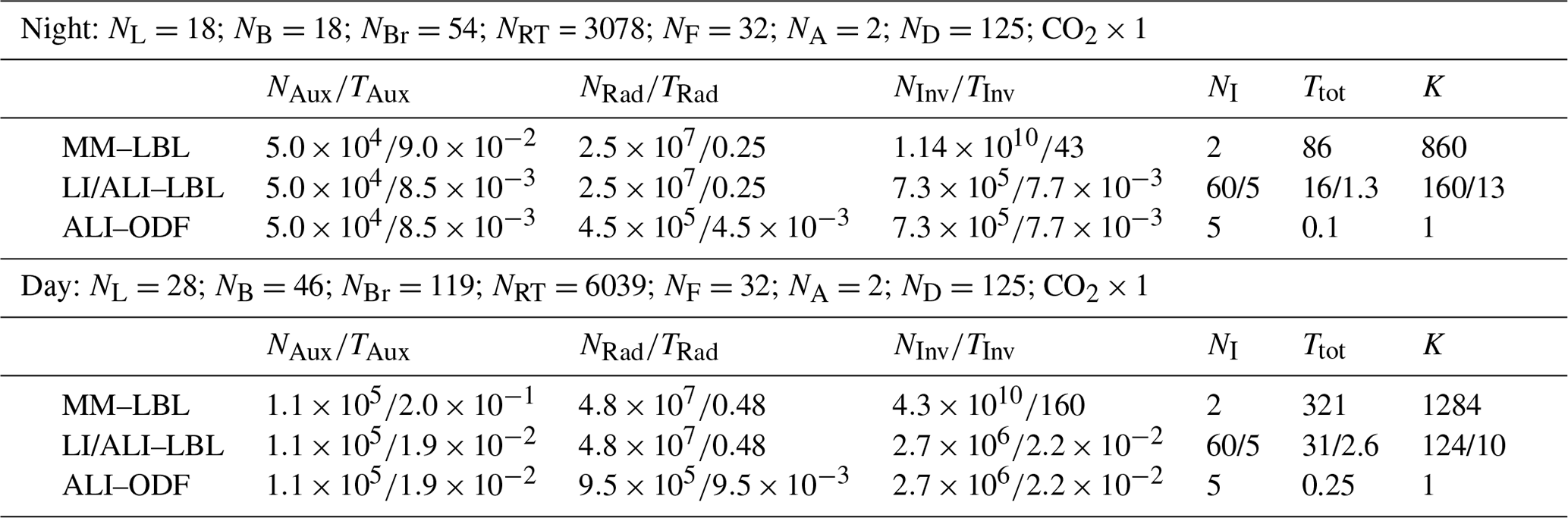
T_Aux, T_Rad, etc. are given in seconds.

In Table 2, we present a summary of our study. The table gives the main parameters of the non-LTE models for day and night conditions described in Sect. 4.1, operation numbers, and the times in seconds (measured with the help of a timing routine within the code), which are required for each calculation part. We performed this study on two different machines, with x86_64 Intel and Intel Xeon Gold processors operating at 2.2 and 2.5 GHz, respectively. We compiled the ALI-ARMS code to be used in 64 bit architecture with the help of a standard GNU Compiler Collection (GCC) compiler, and we ran it on a single processor. We provide the results only for one 2.2 GHz Intel processor; the timing for the second processor is roughly 1.4 times shorter.

Compared to the reference code, we ran the routine using the convergence criterion $\mathrm{1.0}\times {\mathrm{10}}^{-\mathrm{2}}$ instead of $\mathrm{1.0}\times {\mathrm{10}}^{-\mathrm{4}}$. This allowed a reduction in the number of iterations by a factor of about 2 without sacrificing accuracy.

Similarly to the study by Hubeny and Mihalas (2015), we found that the time T required for any procedure like the radiative transfer equation solution or matrix inversion may be presented as

$$\begin{array}{}\text{(4)}& T=CN,\end{array}$$

where N is the number of operations. N is defined by the mathematical nature of the problem and the algorithm applied for its solution. C may, however, depend on many other factors like the quality of programming, language used, operational system, interpreter, computer architecture and performance.

We found that the number of operations for the solution of the radiative transfer equation N_Rad in the case of the non-overlapping lines may be approximated by the expression

$$\begin{array}{}\text{(5)}& N_{\mathrm{Rad}}\simeq N_{\mathrm{D}}\times N_{\mathrm{RT}}\times N_{\mathrm{F}}\times N_{\mathrm{A}}\end{array}$$

and is the same for all algorithms compared. Here N_RT is the total number of lines (or band branches in the ODF case), and N_F and N_A are the numbers of points in the frequency and angle integrals used, respectively. The coefficient C in Eq. (4), which links radiative transfer operation numbers and corresponding times, was found to be $\simeq \mathrm{1.0}\times {\mathrm{10}}^{-\mathrm{8}}$ s.

We found that with the LI/ALI algorithms, the number of auxiliary operations N_Aux is well approximated by the following expression:

$$\begin{array}{}\text{(6)}& N_{\mathrm{Aux}}^{\mathrm{LI}/\mathrm{ALI}}\simeq N_{\mathrm{L}}^{\mathrm{2}}\times N_{\mathrm{D}}.\end{array}$$

This expression gives the number of terms to be filled in the block-diagonal matrix comprising N_D blocks N_L×N_L, where N_L is the number of vibrational levels. In the case of the LI/ALI techniques, these are the N_D matrices generated and inverted one after another at each iteration step. The coefficient C in Eq. (4), which links auxiliary operations and corresponding times, is $C\simeq \mathrm{1.7}\times {\mathrm{10}}^{-\mathrm{7}}$ s.

In the case of the MM technique, the matrix to be generated at each iteration is much larger; namely it has the size $(N_{\mathrm{L}}\times N_{\mathrm{D}})\times (N_{\mathrm{L}}\times N_{\mathrm{D}})$ and consists of N_L fully filled diagonal blocks N_D×N_D, which represent non-local radiative terms, whereas the same as for LI/ALI case collisional terms are now spread over non-diagonal parts of this large matrix. We found that when we present the number of operations to fill this matrix as

$$\begin{array}{}\text{(7)}& N_{\mathrm{Aux}}^{\mathrm{MM}}\simeq N_{\mathrm{D}}^{\mathrm{2}}\times N_{\mathrm{L}},\end{array}$$

then approximately the same coefficient $C\simeq \mathrm{1.7}\times {\mathrm{10}}^{-\mathrm{7}}$ s links this number with the time needed for its filling.

The number of operations needed for matrix inversion N_Inv is approximately N³, where N is the matrix dimension. Thus, we have the following expressions:

$$\begin{array}{}\text{(8)}& N_{\mathrm{Inv}}^{\mathrm{MM}}\simeq (N_{\mathrm{L}}\times N_{\mathrm{D}}{)}^{\mathrm{3}}\end{array}$$

for the MM algorithm and

$$\begin{array}{}\text{(9)}& N_{\mathrm{Inv}}^{\mathrm{LI}/\mathrm{ALI}}\simeq (N_{\mathrm{L}}\times N_{\mathrm{L}}{)}^{\mathrm{3}}\times N_{\mathrm{D}}\end{array}$$

for the LI/ALI techniques. In the latter case the number of operations is $N_{\mathrm{D}}^{\mathrm{2}}$ times lower, since only N_D matrices N_L×N_L are inverted one after another at each iteration. This is the great advantage of these techniques compared to MM, where the entire huge matrix needs to be inverted at once, since it has non-zero elements outside the diagonal blocks.

In the ALI-ARMS code we use ludcmp (lower–upper decomposition), lubksb (back substitution) and mprove (iterative improvement) as matrix inversion routines (Press et al., 2002). We found that, for these routines applied to the non-LTE problems studied here, the coefficient between the number of operations and time for matrix inversion depends on the matrix dimension N and may be approximated by the following expression:

$$\begin{array}{}\text{(10)}& C=\mathrm{1.0}\times {\mathrm{10}}^{-\mathrm{7}}\cdot (\mathrm{0.04}+\mathrm{1.2}/N).\end{array}$$

One may see in the upper part of Table 2 that, for night conditions, the application of the MM technique causes the matrix inversion to be the most time-consuming calculation part at each iteration, although the number of iterations N_Iter=2 is low. Applying LI–LBL techniques provides a strong reduction in the matrix inversion time per iteration but gives only a moderate reduction in the total time (by a factor of ∼5) compared to MM–LBL due to a large number of iterations (60). The number of iterations for the LI/ALI techniques slightly depends on the atmospheric pressure and temperature distribution. The numbers, which are given in the table, are mean values for a few hundreds of runs for different atmospheric conditions. Applying ALI instead of LI significantly reduces the number of iterations (5 instead of 60), providing additional acceleration of calculations by a factor ≳10. We note that for LI/ALI–LBL, the most time-consuming part for each iteration is now the radiative transfer solution, which is more than 15 times slower than two other parts of calculation together. The ODF technique allows a reduction in T_Rad by a factor of 50–60. This provides total additional acceleration by a factor of ≳10. The last column in the table gives the acceleration factor $K=T_{\mathrm{tot}}/T_{\text{tot,\hspace{0.17em} ALI–ODF}}$, which shows how much faster the ALI–ODF combination works compared to other techniques: it is about 900 and 160 times faster than the MM–LBL and LI–LBL techniques, respectively.

The lower part of Table 2 shows the number of operations and times for various parts of calculations for the daytime non-LTE model described in Sect. 4.1. Compared to the nighttime, daytime calculations require about 2.5 times more time due to an increased number of vibrational levels and bands accounted for. Nevertheless, the main points discussed above in this section for the nighttime runs remain valid for the daytime: (a) the main decelerating factor for the MM technique is the matrix inversion, notwithstanding the low number of iterations; (b) the LI technique, although it reduces the matrix inversion time by a factor of ≳7000, provides only a moderate decrease in total time (by a factor of ∼ 10) because of the large number of iterations; (c) the ALI technique is more than 100 times faster than MM, with the slowest part of calculations being the LBL solution of RTE; and (d) the ODF provides acceleration of radiative transfer calculations by a factor of 50. Finally, the ALI–ODF technique appears to be over 1000 times faster than the MM–LBL approach.

We measured the time the F98 routine requires on x86_64 Intel 2.2 GHz processors and found it to be around $\mathrm{3}\times {\mathrm{10}}^{-\mathrm{4}}$ s. This means that for the nighttime, KF23 is about 300 times slower than F98. In the daytime, when the solar heating parameterization of Ogibalov and Fomichev (2003)) is accounted for, our version of F98 requires about 30 % more time. Still, it remains about 600 times faster than the daytime KF23 routine. In the next section we discuss in detail the accuracy of both routines.

5 Accuracy of cooling–heating rate calculations

To estimate the calculation errors, we compared the outputs of our new KF23 routine and the F98 routine for the non-LTE CO₂ cooling calculations with our non-LTE reference model, discussed in Sect. 4.1. In these tests, we used the CO₂ volume mixing ratio (VMR) profiles with 400 ppmv in their “well-mixed” part. We also tested the same profiles multiplied by factors of 2, 4 and 10. For the CO₂(ν₂)+O(³P) quenching rate, we used the temperature-dependent coefficient $k=\mathrm{3.0}\times {\mathrm{10}}^{-\mathrm{12}}$ s⁻¹ cm³ × $\sqrt{(T/\mathrm{300})}$ (see Sect. 5.4 for more details). As we described before in Sect. 4.1, the vibrational levels and bands accounted for in KF23 keep their accuracy of ∼ 1 K d⁻¹ for any temperature profile, including those strongly disturbed by various tidal and gravity waves. Here, we show the cooling rates calculated using both routines compared to the cooling rates obtained using the reference model only for “wavy” temperature profiles. For mean profiles with a smooth structure, the errors of KF23 were about 0.1–0.3 K d⁻¹ (for 400 ppmv of CO₂). For the F98 routine, the errors for smooth profiles were around 1–3 K d⁻¹, confirming the results of Fomichev et al. (1998).

5.1 The nighttime cooling–heating rates

In Fig. 2, we show five typical temperature profiles, which demonstrate the superposition of different meso-scale waves. These profiles, as well as corresponding pressure, O(³P) and CO₂ distributions (shown in Fig. 3), and other constituents from the Whole Atmosphere Community Climate Model Version 6 (WACCM6) (Gettelman et al., 2019) runs were kindly provided by Daniel Marsh (personal communication, 2022). For the 15 µm cooling calculations, this model uses the F98 parameterization. We show below the calculation results for these atmospheric model inputs because WACCM is widely used by the model community. Generally, any pressure/temperature profiles disturbed by strong waves give similar results, as we observed in our tests. These may be p–T distributions generated by modern GCMs, like in our case here; those retrieved from ground-based or space observations; or artificial wavy p–T distributions.

Figure 2 Temperature profiles used for testing the CO₂ 15 µm cooling calculations.

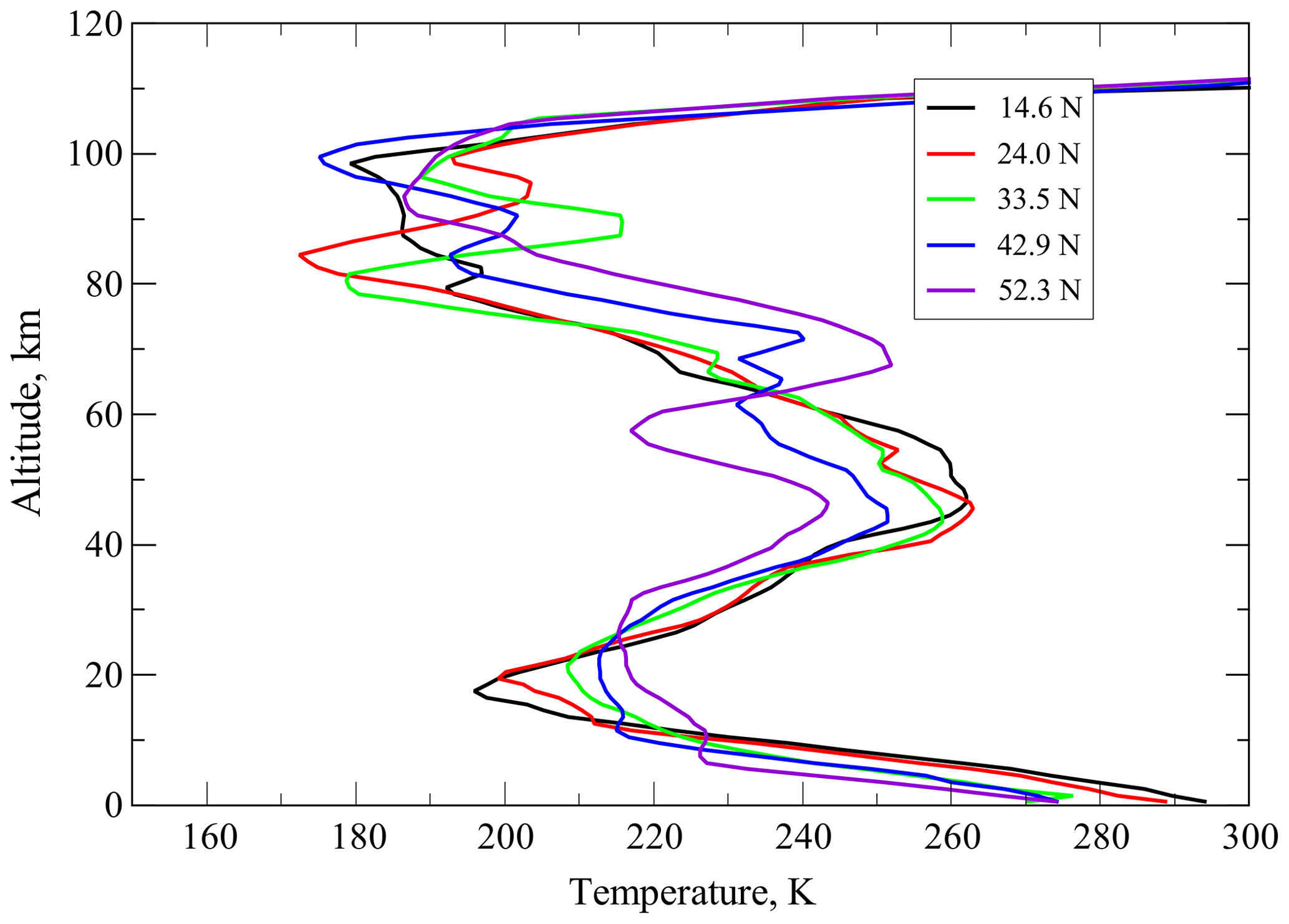
Figure 3 Volume mixing ratio profiles of CO₂ and O(³P) used for testing the CO₂ 15 µm cooling calculations. Solid magenta line with diamonds for 0.0° N are data taken from Yudin et al. (2022) which were used for the simulations shown in Fig. 9; solid lines for 14.6–52.3° N correspond to the temperature profiles in Fig. 2 and were used for simulations shown in Figs. 4–6; see text for details.

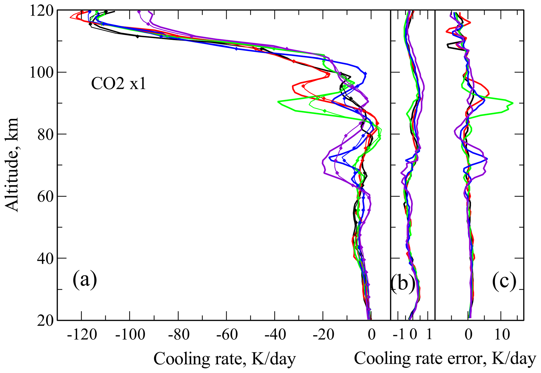
Figure 4 The nighttime cooling rates in the CO₂ 15 µm band and cooling rates errors for the CO₂ VMR of 400 ppmv for temperature distributions of Fig. 2. Line colors correspond to the legend in Fig. 2. (a) Cooling rates: thick solid lines – reference model; thin solid lines with diamonds – F98 routine; the KF23 results are not shown; (b) Cooling rate differences between the new routine KF23 and reference data; (c) Cooling rate differences between the F98 routine and reference data.

Figure 4 shows the CO₂ 15 µm cooling rates for the new KF23 routine, for the F98 parameterization, and for our reference non-LTE model for temperatures in Fig. 2 and the 400 ppmv CO₂ profiles. One may see in this figure that the new routine errors do not exceed 0.5 K d⁻¹. On the other hand the F98 routine errors reach up to 13 K d⁻¹. The altitude range, where the F98 routine demonstrates significant errors, is broad starting just above the altitude of 60 km.

Figure 5 The same as in Fig. 4, however, for 800 ppmv of CO₂.

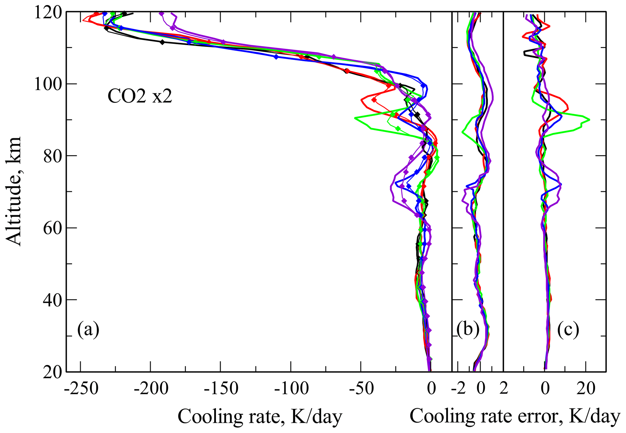
In Fig. 5 we show the same as Fig. 4 – cooling rates and their differences – but for the twice higher CO₂ of 800 ppmv in the well-mixed range. We note here that both maximal absolute values of cooling rates and the new and the F98 routine errors are roughly twice higher compared to those of Fig. 4. For the new routine they do not exceed 1 K d⁻¹, whereas for the F98 routine they reach up to 23 K d⁻¹.

Figure 6 The same as in Fig. 4, however, for 4000 ppmv of CO₂, no results for the F98 routine are shown.

Finally, in Fig. 6, we show in panel (a) the cooling rates produced by the reference model and by the KF23 routine for the CO₂ VMR of 4000 ppmv, which is 10 times higher than the reference one. The new routine errors are shown in panel (b). The F98 routine was not tested for these inputs, since it was not designed to work with the CO₂ VMRs higher than 720 ppmv. One may see in this figure that absolute cooling rates (maximal values) are approximately 10 times higher than those for 400 ppmv of CO₂. The same is roughly true for the new routine errors, which now reach values of up to 8 K d⁻¹ in upper parts of the tested region.

Figure 7 Contributions of various CO₂ bands to the total nighttime cooling at 33.5° N. The narrow sub-panels show re-scaled 626 isotope hot bands and minor isotope contributions.

In Fig. 7 for night, we show the contributions of major and minor CO₂ isotopes included in the model (see Sect. 4.1), for a temperature at 33.5° N for 400 and 1600 ppmv of CO₂. One may see in this figure that, for the 400 CO₂ ppmv, this contribution does not exceed ∼ 2 and ∼1 K d⁻¹ for the 626 hot bands and for all minor isotope bands, respectively. This effect of hot bands and minor species is increasing with the CO₂ density; see the right panel of Fig. 7, particularly for altitudes affected by waves.

As we mentioned in Sect. 4.1, we use all CO₂ bands available in HITRAN2016 for the night set of levels in Table 1. This minimizes errors compared to reference calculations to ≤1 K d⁻¹ for 400 ppmv of CO₂. The routine allows for using fewer levels and bands to accelerate calculations but at the expense of error increase (see Appendix A for more details). For instance, excluding (see Fig. 1) weak first hot bands, (10001,02201,10002)→01101, and second hot bands, (11101,03301,11102)→(10001,02201,10002), of 626 and 636 isotopes makes the total number of bands twice lower. Our tests show that in this case the routine works only about 10 % (see also Table 2) faster; however the maximal cooling rate error for 400 ppmv increases to up to 3 K d⁻¹.

5.2 The daytime cooling–heating rates

In the daytime, the near-infrared heating due to the absorption of solar radiation in the CO₂ bands around 2.0–4.3 µm represents a small but non-negligible reduction in the total CO₂ cooling (up to 1–2 K d⁻¹ for the current CO₂). The complex mechanisms of the absorbed solar energy assimilation into heat have been investigated in detail in a number of studies summarized by López-Puertas and Taylor (2001). Ogibalov and Fomichev (2003) studied this heating for smooth temperatures for various CO₂ densities and solar zenith angles (SZAs) and suggested the use of a lookup table, which allows a quick estimate of this heating in GCMs. Due to its reasonable accuracy (∼ 0.5 K d⁻¹ for current CO₂), this table has been used as a daytime supplement to the F98 nighttime cooling parameterization. Unfortunately, with increasing CO₂ density, the errors in this table increase rapidly above ∼ 70 km: for 720 ppmv CO₂ it underestimates the heating around the mesopause by more than 50 % (see Fig. 5 of Ogibalov and Fomichev, 2003, for daily averaged heating).

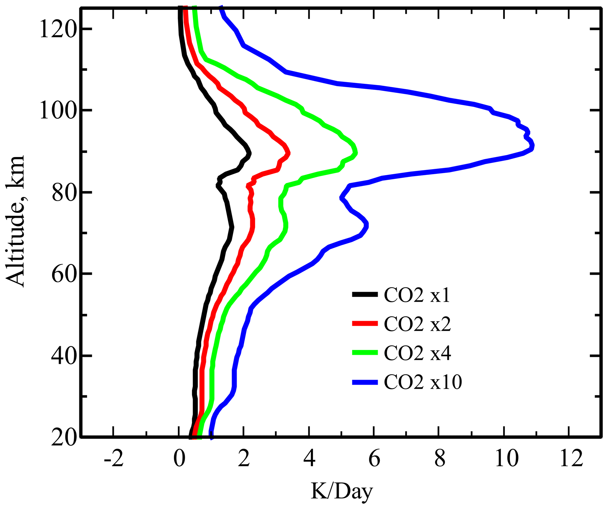
Figure 8 The near-infrared solar heating at 33.5° N for solar zenith angle 45° for various CO₂ densities.

In Fig. 8 the heating of the atmosphere due to the daytime absorption of solar radiation in the CO₂ bands at 2.0–4.3 µm for SZA = 45° at 33.5° N produced by our new routine is shown. To prevent increasing errors for the daytime due to an inadequate treatment of solar radiation absorption and assimilation, KF23 utilizes, in the daytime, an extended non-LTE model which, compared to the nighttime, includes 10 more CO₂ vibrational levels (see Table 1) and a comprehensive system of radiative and collisional VT and VV energy exchanges as described by Shved et al. (1998) and Ogibalov et al. (1998). A higher number of vibrational levels and more than twice the number of bands lead to a 2.5-fold longer time for the daytime cooling–heating calculation (see Table 2). However, the daytime errors are of the same order of magnitude (less than 1 K d⁻¹ for 400 ppmv) as those for the nighttime (Figs. 4–6) even for strongly perturbed temperatures and increased CO₂. We do not present these comparisons. As in the night case, removing half of bands (various hot and combinational bands) in the daytime model gives only about 10 % speed gain; however, for 400 ppmv, maximal errors in cooling may reach 4 K d⁻¹.

5.3 Cooling–heating rates for the diurnal tides at Equator

In Fig. 9, we compare the cooling rates obtained with the KF23 routine and with F98 parameterization with those produced by the reference model. For these tests, we used the temperature–pressure distributions affected by the diurnal tides at the Equator; p, T and the atmospheric constituent densities as well as local zenith angles for local times at 1.0° N and 12.0° E (15 March 2019) correspond to the WACCM-X (Whole Atmosphere Community Climate Model with thermosphere and ionosphere extension) equatorial simulations constrained by meteorological analyses of the NASA Goddard Earth Observing System version 5 (GEOS-5) below the stratopause, as discussed in Yudin et al. (2020, 2022). The temperature distributions at various local times are shown in panel (a). Panel (b) presents the CO₂ 15 µm cooling rates calculated using the reference model (thick solid lines) and the F98 routine (thin solid lines with diamonds). We do not show here the cooling rates obtained using the KF23 routine because the difference between them and the reference data does not exceed 1 K d⁻¹ ; see Fig. 9c. Figure 9d shows the differences between the cooling produced by the F98 routine and the reference calculations. In contrast to Fig. 9c, these differences exceed 20 K d⁻¹ for some temperature profiles.

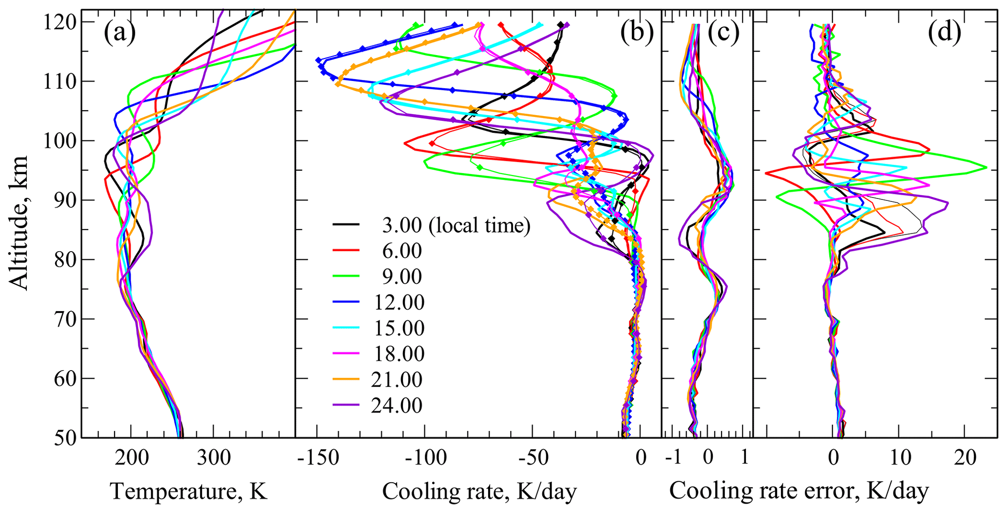
Figure 9 Comparisons of the CO₂ 15 µm cooling rates. Diurnal tides at the Equator. (a) Temperature profiles for various local times. (b) Cooling rates: thick solid lines – reference model, thin solid lines with diamonds – F98 routine. (c) Cooling rate differences between the new routine, presented in this study, and the reference model. (d) Cooling rate differences between the F98 routine and the reference model.

One may see in Fig. 9 that the accuracy of the F98 routine improves above 100 km and below 80 km. Above 100 km, the F98 parameterization uses a recursive expression, the accuracy of which increases with height (Kutepov, 1978). Below 80 km, the F98 routine is based on the LTE matrix algorithm for cooling calculations. This algorithm accounts for the radiative interaction of the neighboring levels and the escape of radiation to above and, therefore, provides a good accuracy of cooling in this optically thick layer. In the layer between 80 and 100 km, the F98 routine merges the cooling values calculated by the two methods outlined above. This merging works reasonably well for smooth temperature distributions tested by Fomichev et al. (1998), but it fails with wavy temperatures. One also needs to keep in mind that this layer is the transition region between the LTE and non-LTE state of the CO₂(ν₂) vibrations, where the physics of formation of the non-equilibrium vibrational distribution must be considered in all aspects (e.g., Kutepov et al., 2006). Compared to the KF23 routine, which rigorously models the non-LTE, the F98 routine fails in this situation, which Fomichev et al. (1993) warned about when they presented the first version of this parameterization.

5.4 The CO₂(ν₂)+O(³P) quenching rate coefficient

The results above in Sect. 5.1–5.3 were obtained for the temperature-dependent CO₂(ν₂)+O(³P) quenching rate coefficient $k=\mathrm{3.0}\times {\mathrm{10}}^{-\mathrm{12}}$ s⁻¹ cm${}^{\mathrm{3}}\times \sqrt{(T/\mathrm{300})}$. The multiplier in this expression is the median value of the rate coefficient from the range of (1.5–6.0) $\times {\mathrm{10}}^{-\mathrm{12}}$ s⁻¹ cm³, which spans the low laboratory data up to high data obtained from the space observations of the CO₂ 15 µm emission; see, for example, Feofilov et al. (2012), and references therein. This value is currently accepted for usage in the GCMs for calculation of the 15 µm cooling. The dependence of MLT cooling on k has been investigated in many previous works summarized by López-Puertas and Taylor (2001, and also references therein). It is known that the maximum value of cooling, which is usually reached at the altitudes of 100–140 km, is roughly proportional to the k value used in calculations. The KF23 routine works well for any k value from the range given above, and it also allows varying the temperature dependence of the rate coefficient (e.g., Castle et al., 2012); see Appendix A. For our calculations, we used the O(³P) densities shown in Fig. 3.

5.5 Upper and lower boundaries

The accuracy tests of the KF23 routine were performed with the upper boundary of the atmosphere at 130 km. The routine may work with any upper boundary in the upper mesosphere and above. Putting the upper boundary below ∼ 110 km may cause, however, increasing cooling errors due to not accounting for the upper atmospheric layers. The lower boundary can be placed at any altitude below ∼ 50 km where all CO₂ 15 µm bands are in LTE. This will justify the LTE lower boundary condition for the radiative transfer equation solution. However, it is not recommended to use the routine results below ∼ 20 km because of increasing errors by not accounting for the line overlapping in a current version of the ODF approach.

6 Conclusions

We present the new KF23 routine for calculating the non-LTE CO₂ 15 µm radiative cooling–heating in the middle and upper atmosphere. The routine provides high-accuracy cooling rates above 20 km in a broad range of atmospheric input variations for any temperature distributions including those disturbed by strong micro- and meso-scale strictures and is the optimized version of the ALI-ARMS reference model and research code (Feofilov and Kutepov, 2012), which rigorously solves the non-LTE in CO₂, N₂ and O₂ coupled by intensive vibrational–vibrational energy exchanges. The routine relies on advanced techniques of exact non-LTE problem solutions (ALI algorithm) and the molecular band radiative transfer treatment (ODF technique). Using these algorithms, we have sped up the cooling rate calculation by about 1000 times compared to the standard matrix and line-by-line technique of the same non-LTE problem solution. We show that the maximum error in calculations does not exceed 1 K d⁻¹ for the current atmospheric CO₂ density and the median value of CO₂(ν₂)+O(³P) quenching rate coefficient. This accuracy is ensured by a relatively large number of CO₂ levels and bands used in the KF23 routine. We also allow the user to choose between the accuracy and calculation speed by adding or removing certain bands and levels (see Appendix A).

The KF23 routine provides accurate cooling calculations in a vast range of the CO₂(ν₂)+O(³P) quenching rate coefficient and O(³P) variations. It also works well for very broad variations in the CO₂ VMR, both below and above the current density, up to 4000 ppmv. Consequently, this allows the application of this routine in models of Earth's ancient atmospheres and models of climate changes caused by increasing CO₂.

Recently López-Puertas et al. (2024) presented an updated version of the F98 routine. Detailed analysis of this work is given by Kutepov (2023). The main improvement of the revised routine (hereafter F24) compared to F98 is an extended range of CO₂ abundances: whereas the F98 routine covered the range of CO₂ concentrations with tropospheric values from 150 to 720 ppm, F24 goes up to 3000 ppm of tropospheric CO₂. Another minor improvement is the finer altitude grid of revised parameterization. The authors show numerous tests of the routine accuracy but only for undisturbed individual temperature distributions, for which its error does not exceed 0.5 K d⁻¹. They also tested the revised routine for the temperatures retrieved from MIPAS (Michelson Interferometer for Passive Atmospheric Sounding) observations, which demonstrate large variability. These individual profiles are good inputs for the revised parameterization to show how it works for strongly disturbed temperature profiles. However, the authors do not show these results. Instead, they present only zonal means of the differences. Obviously, this averaging washes out the errors obtained for individual profiles, for which we observed (see Sect. 5) the F98 parameterization errors up to 25 K d⁻¹. Meanwhile these large errors are generally concentrated in the altitude region around 90 km, exactly where the root mean square errors (RMSEs) of F24 in López-Puertas et al. (2024) are maximized, reaching 8–9 K d⁻¹. In Sect. 5 we explain why F98 works badly in this altitude region. These large RMSEs allow us to conclude that the revised routine presented by López-Puertas et al. (2024) has the same problems as the F98 parameterization. We compared F24 with our routine for the same wavy profiles using the collisional quenching rates we applied this work for testing F98. We found that maximal errors of F24 for these profiles are about 30 % lower than those of F98. However, this improvement in the calculation accuracy of F24 was achieved by increasing the calculation time by approximately 2.4 times. López-Puertas et al. (2024) reported that F24 worked 6600 times faster than our procedure KF23 comparing the calculation time of KF23 for night taken from Table 2 of this paper with the calculation time of F24, which they obtained when using a significantly faster processor. We compared the performance of F24 and KF23 routines as described in Sect. 4.2. This comparison showed that F24 is only about 125 and 250 times faster than KF23 for night and day, respectively.

Appendix A: The NLTE15µmCool-E v1.0 routine (technical details)

The routine source code is written in C. The routine is available at https://doi.org/10.5281/zenodo.8005028 (Kutepov and Feofilov, 2023) and is ready for implementation into any general circulation model usually written in Fortran through a small “wrapper”.

The routine has an interface, which allows efficiently receiving feedbacks from the model. These are inputs required for the cooling calculations such as pressure, temperature, CO₂, O(³P) and other atmospheric constituent densities. It returns the CO₂ 15 µm radiative cooling–heating according to the altitude grid specified by the user. The routine works for day (SZA ≤110°) and night (SZA > 110°) conditions.

Following the discussion in Sect. 5, the routine may generally work with any upper and lower boundary; however it is not recommended to put the upper boundary below ∼ 110 km, since this causes increasing calculation errors due to not accounting for the upper atmospheric layers, or to place the lower boundary below ∼ 20 km because of increasing errors caused by not accounting for the line overlapping in the current version of the ODF approach.

The module requires geometrical altitudes to calculate radiative transfer and an equidistant altitude grid, which guaranties the exact solution of the radiative transfer equation. The user may define any grid step including very fine ones, which allows the resolution of micro-scale temperature disturbances. This is an advantage of our routine, since its calculation time only linearly depends on the number of grid points N_D. Compared to this, the calculation time of matrix algorithms is $\sim N_{\mathrm{D}}^{\mathrm{3}}$; see Eqs. (4)–(10). Nevertheless, for those who want to account for the additional cooling effect of the micro-scale sub-grid disturbances, we recommend using its parameterization described in Kutepov et al. (2007) and Kutepov et al. (2013b), which may be easily implemented in the routine.

The routine includes all inputs required for its proper performance, among them all collisional rate coefficient parameterizations as described by Shved et al. (1998) as well as the HITRAN2016 spectroscopic data for all bands available for the CO₂ level set in Table 1. The latter are presented as temperature-dependent A(T) and B(T) Einstein coefficients for each band branch calculated in accordance with Kutepov et al. (1998) and Gusev and Kutepov (2003). We compared A(T) and B(T) with those calculated for two earlier HITRAN versions and found the differences to be less than 0.1 %–0.2 % for bands included in our CO₂ nighttime model. For some hot 15 and 4.3 µm and combinational bands included in the daytime model, these differences are of the order of 0.5 %, since data for these bands slightly vary from one HITRAN version to another.

The routine also includes a detailed table of basic ODF for a band branch in a broad range of temperature and pressure variations. This ODF is re-scaled in a special way onto the ODF for each individual band branch.

The supplied set of levels and spectral band information ensures the cooling–heating calculation errors for day and night to be below 1 K d⁻¹ for any temperature profile. For smooth temperature profiles, the calculation errors are around 0.1–0.3 K d⁻¹ (for 400 ppmv of CO₂).

Finally, the routine allows the user to switch on and off the vibrational levels and/or bands used in the model. This removing or adding of vibrational levels will also automatically add (or remove) the bands related to these levels. If the user task can tolerate larger errors, the calculation speed can be increased at the cost of lowering the accuracy.