Deep learning model based on multi-scale feature fusion for precipitation nowcasting

Forecasting heavy precipitation accurately is a challenging task for most deep learning (DL)-based models. To address this, we present a novel DL architecture called “multi-scale feature fusion” (MFF) that can forecast precipitation with a lead time of up to 3 h. The MFF model uses convolution kernels with varying sizes to create multi-scale receptive fields. This helps to capture the movement features of precipitation systems, such as their shape, movement direction, and speed. Additionally, the architecture utilizes the mechanism of discrete probability to reduce uncertainties and forecast errors, enabling it to predict heavy precipitation even at longer lead times. For model training, we use 4 years of radar echo data from 2018 to 2021 and 1 year of data from 2022 for model testing. We compare the MFF model with three existing extrapolative models: time series residual convolution (TSRC), optical flow (OF), and UNet. The results show that MFF achieves superior forecast skills with high probability of detection (POD), low false alarm rate (FAR), small mean absolute error (MAE), and high structural similarity index (SSIM). Notably, MFF can predict high-intensity precipitation fields at 3 h lead time, while the other three models cannot. Furthermore, MFF shows improvement in the smoothing effect of the forecast field, as observed from the results of radially averaged power spectral (RAPS). Our future work will focus on incorporating multi-source meteorological variables, making structural adjustments to the network, and combining them with numerical models to further improve the forecast skills of heavy precipitations at longer lead times.

1 Introduction

Heavy precipitation can cause various natural disasters, such as floods, landslides, and mud–rock flows, which can be life-threatening and cause property damage. Nowcasting is the term used for predicting precipitation in a specific region within a short time frame (usually less than 3 h) and with a high spatiotemporal resolution (Ayzel et al., 2020; Czibula et al., 2021). It has become a popular research topic in hydrometeorology. The intensity, duration, and area of precipitation determine the extent of its destruction. Consequently, accurate and timely nowcasting is essential for disaster early warning and emergency response (Chen et al., 2020; Ehsani et al., 2021). However, real-time, large-scale, and fine-grained precipitation nowcasting remains a challenging task due to the complexities of atmospheric conditions (Ehsani et al., 2021; Kim et al., 2021).

There are two main conventional approaches for precipitation nowcasting: numerical weather prediction (NWP)-based methods (Sun et al., 2014; Yano et al., 2018) and radar echo-based quantitative forecasts (Liguori et al., 2014). The NWP models predict precipitation dynamics by solving a series of differential equations to describe atmospheric phenomena (Dupuy et al., 2021), but they are computationally intensive and time-consuming, and their forecast products depend on initial and boundary conditions (Marrocu et al., 2020; Ehsani et al., 2021). Moreover, the first few hours of precipitation predictions by NWP models are invalid, so they are not commonly used in nowcasting (Han et al., 2019; Yan et al., 2020). On the other hand, radar echo-based quantitative models use the Z−R relationship to drive precipitation rates and estimate precipitation accumulations. The optical flow model is the simplest technique in radar echo-based quantitative forecast models, which consists of tracking and extrapolation. In this technique, an advection field is estimated from a series of consecutive radar echo images, and it is then used to extrapolate recent radar echo images through semi-Lagrangian schemes or interpolation procedures (Ayzel et al., 2019). Many studies have documented the progress and achievements in precipitation nowcasting with variations of the OF model (Marrocu et al., 2020; Pulkkinen et al., 2019; Ayzel et al., 2019; Prudden et al., 2020; Liu et al., 2015; Woo and Wong, 2017; Li et al., 2018). However, the OF model has certain limitations due to the assumption of a constant advection field (Prudden et al., 2020; Li et al., 2021).

In recent years, deep learning (DL) techniques have become increasingly popular for precipitation nowcasting, due to their superior performance in tracking and processing successive frames of radar echo video/images. For instance, Shi et al. (2015) treated precipitation nowcasting as a spatiotemporal sequence predictive problem and proposed a convolutional long short-term memory (ConvLSTM) architecture, which captures spatial and temporal features of radar echo sequences. This model outperformed the OF method. In their follow-up study (Shi et al., 2017), they introduced a trajectory GRU (TrajGRU) model, which used the same convolutional and recursive networks as the ConvLSTM while excavating the spatially variant relationship of radar echo through its sub-networks. Moreover, Chen et al. (2020) built a new architecture with a transition path (star-shaped bridge (SB)) based on ConvLSTM, which gleans more latent features and makes the model more robust. The model was tested in precipitation nowcasting over the Shanghai area and achieved better performance than some conventional extrapolation methods. To improve the limitation of time-step reduction in the ConvLSTM model, Yasuno et al. (2021) proposed a rain-code approach with multi-frame fusion, allowing the model to have a forecast lead time of 6 h. Ronneberger et al. (2015) presented a U-shaped architecture deep network, namely UNet, consisting of a contracting path to capture context and an expanding path that enables precise positioning. This model was initially used in biomedical segmentation applications. Numerous attempts have been made to develop a UNet-based precipitation nowcasting model, including the “RainNet” in Germany (Ayzel et al., 2020), the “MSDM” in eastern China (Li et al., 2021), the “Convolutional Nowcasting-Net” with IMERG products (Ehsani et al., 2021), the “SmaAt-UNet” in the Netherlands (Trebing et al., 2021), the “FURENet” for convective precipitation nowcasting (Pan et al., 2021), and the nowcasting system with ground-based radars and geostationary satellite imagery (Lebedev et al., 2019). Additionally, Sadeghi et al. (2020) used a UNet convolutional neural network and geographical information to enhance near real-time precipitation estimation.

When it comes to radar-based nowcasting, there are several plug-and-play modules available that use different network architectures. Some models use ConvLSTM or UNet-based architectures, while others either trim deformable network architectures or implant various feature extraction operations into the network architectures. For instance, Ravuri et al. (2021) proposed a conditional generative model for probabilistic nowcasting. Their model produced realistic and spatiotemporally consistent predictions with a lead time of up to 90 min, outperforming UNet and PySTEPS (Pulkkinen et al., 2019). The Google Research group (Sønderby et al., 2020) developed “MetNet”, a weather probabilistic model that uses axial self-attention mechanisms to unearth weather patterns from large-scale radar and satellite data. The model provided probabilistic precipitation maps for up to 8 h over the continental United States at a spatial resolution of 1 km and a temporal resolution of 2 min. The Huawei Cloud group (Bi et al., 2023) devised a 3D earth-specific transformer module and developed “Pangu-Weather”, a high-resolution system for global weather forecasting. This system showed good application prospects for its superior performance in many downstream forecast tasks such as wind, temperature, and typhoon forecasts. Researchers from DeepMind and Google (Lam et al., 2023) proposed a novel machine learning weather simulator named “GraphCast”. It was an autoregressive model based on graph neural networks and a high-resolution multi-scale mesh representation, which produced medium-range global weather forecasting for up to 10 d. The Microsoft Research Group developed and demonstrated the “ClimaX” model (Nguyen et al., 2023). This model extended the transformer architecture with novel encoding and aggregation blocks, resulting in superior performance on benchmarks for both weather forecasting and climate projections. Similarly, Chen et al. (2023) presented an advanced data-driven global medium-range weather forecast system named “FengWu”. This system was equipped with model-specific encoders–decoders, a cross-modal fusion transformer, and a replay buffer mechanism. It solved the medium-range forecast problems from a multi-modal and multi-task perspective. Marrocu et al. (2020) proposed the “PreNet” model, which was based on a widely used semi-supervised and unsupervised learning DL method named “generative adversarial network” (GAN) (Goodfellow et al., 2014). The model's performance was compared with state-of-the-art OF procedures and showed remarkable superiority. Zheng et al. (2022) established the “GAN-argcPredNet” model, which was also based on GAN architecture. It can reduce the prediction loss in a small-scale space and show more detailed features among prediction maps.

However, DL-based models for precipitation nowcasting have their limitations and challenges, as reported by various studies (Ayzel et al., 2020; Chen et al., 2020; Ehsani et al., 2021; Prudden et al., 2020; Su et al., 2020; Li et al., 2021; Kim et al., 2021; Singh et al., 2021; Huang et al., 2023). First, these models struggle to extrapolate short-term local convection or precipitation fields due to the complex nature of precipitation dynamics and the fact that DL models rely solely on historical radar echo data to learn prior knowledge (Su et al., 2020; Chen et al., 2020; Ehsani et al., 2021). This makes it challenging to predict fast-moving precipitation systems or short-term local convections characterized by rapid growth and dissipation. Second, iterative forecasts tend to result in accumulative errors and uncertainties due to discrepancies between the model's training and testing processes (Ayzel et al., 2020; Prudden et al., 2020; Li et al., 2021; Singh et al., 2021; Huang et al., 2023). This can lead to low values of heavy precipitation, smoothing, or blurry forecast fields. Third, the convolution operation used in DL models covers precipitation fields as comprehensively as possible, but it cannot reveal the rapid changes in echo intensity, deformation, and movement of precipitation fields (Ehsani et al., 2021; Kim et al., 2021). Consequently, DL models produce some undesirable forecast outputs, such as declining forecast skills with increasing lead time, smoothing and blurry precipitation fields, missing extreme precipitation events, and poor forecast skills for precipitation growth and dissipation.

Large-scale precipitation systems are influenced by several factors, including prevailing westerlies, trade-wind zones, mesoscale weather systems, land–sea distributions, and topography effects (Huang et al., 2023; Luo et al., 2023). As a result, real-time and accurate precipitation forecasting remains a challenging task. In this study, we utilized large-scale radar echo data and designed a DL architecture called “multi-scale feature fusion” (MFF). The MFF model focuses on detecting multi-scale features of radar echoes, such as intensity, movement direction, and speed, which is expected to enhance precipitation forecasting skills, particularly in predicting precipitation growth and dissipation, fast-moving precipitation systems, and heavy precipitations. This article is organized as follows: Sect. 2 presents the data materials, the detailed method, and the framework of the model. Section 3 describes the experimental results from two precipitation cases and discusses the advantages and disadvantages of the four models. Finally, Sect. 4 concludes the study and explores possible future work.

2 Materials, methods, and models

2.1 Radar reflectivity image products

Weather radar is a crucial tool for monitoring precipitation systems and severe convective weather events such as hail, gales, tornadoes, and flash floods. As of November 2022, the China Meteorological Administration has installed a network of 236 C-band and S-band Doppler weather radars across China, known as the China Next Generation Weather Radar (CINRAD) network (see Fig. 1). However, the CINRAD network is distributed heterogeneously across China except in complex terrain (Min et al., 2019). The network measures the speed of meteorological targets relative to the radars and then produces various types of meteorological products. This study focuses on collecting and organizing radar reflectivity image products from five seasons (March to August) between 2018 and 2022. The data have a temporal resolution of 6 min and covers an area over (73–135^∘ E, 10–55^∘ N). The data pre-processing steps include the following:

1. Low-altitude objects, such as mountains, buildings, and trees, can produce sham echoes in radar images. Therefore, we remove these anomalous radar echoes and detach unnecessary annotations like city names, demarcations, and rivers from each image. To reduce the impact of sham echoes on the extrapolative model, we use a local-mean filter algorithm to denoise the radar images. After this, we transform the radar reflectivities into precipitation values using the Z−R relationship.

2. The extrapolative model is difficult to converge because of the significant numerical differences among each echo reflectivity. As a result, we normalize the initial radar reflectivities to a range of [0,1]. Also, to assign precipitation values in areas without radar echo, we set them as 0. Finally, we resample the precipitation values on a 1024×880 grids for each radar image. The spatial resolution of one radar image, combining all grid boxes, is approximately 5 km. After completing the data preprocessing steps, we obtained 205 848 samples, which is a 3D matrix with the size of $[\mathrm{205}\mathrm{848}\times \mathrm{1024}\times \mathrm{880}]$.

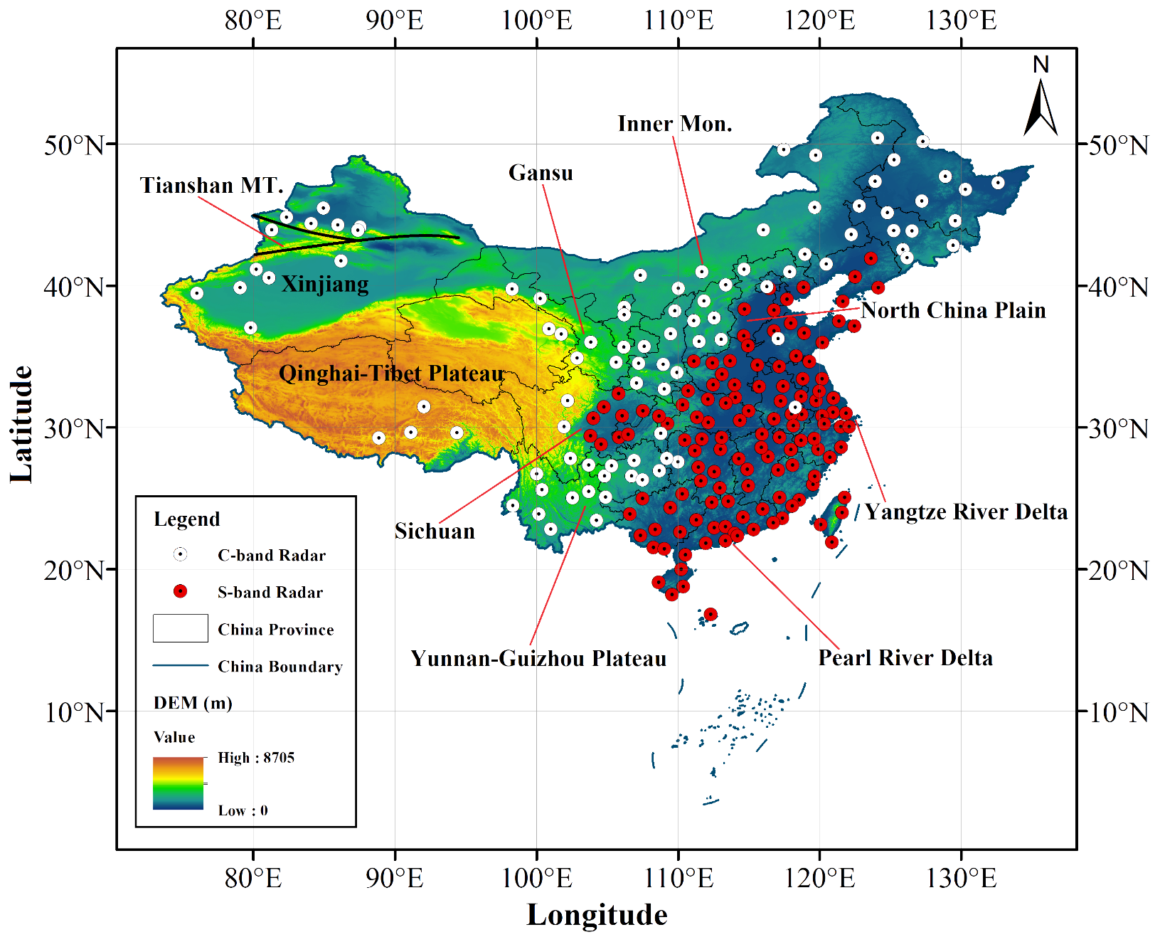
Figure 1 The distribution of the CINRAD over China and Topography (in meters) map. White dots represent C-band radars and red dots denote S-band radars.

2.2 Multi-scale feature fusion

Radar echo extrapolation is an important technique for predicting precipitation by analyzing key variables such as convective cloud intensity, shape, movement direction, and speed. However, echo images may have different targets such as light rain, moderate rain, and heavy rain, or the same target may vary in size at different resolutions. Additionally, in a specific area of interest in an echo map, there may be multiple targets arranged in a tight or disorderly manner, which can cause background noise, particularly due to strong local convection. Therefore, using a single feature or convolution kernel in a deep learning architecture can lead to lower forecasting accuracy due to the limited receptive field.

This study introduces two modules for feature fusion: a 3D multi-scale feature fusion (3DMFF; Fig. 2a) module and a 2D multi-scale feature fusion (2DMFF; Fig. 2b) module. The 3DMFF module uses convolution kernels of different sizes to capture information from different receptive fields. Assuming that the average moving speed of a convective cloud is 36 km h⁻¹, the largest convolution kernel with the size of $\mathrm{4}\times \mathrm{5}\times \mathrm{5}$ grid can capture the traceability information of the convective cloud under this moving speed. Conversely, the smallest convolution kernel with the size of $\mathrm{4}\times \mathrm{2}\times \mathrm{2}$ grid is geared toward the slow-moving clouds. Additionally, a kernel with the size of $\mathrm{4}\times \mathrm{1}\times \mathrm{1}$ grid is used for dimensionality adjustments and information interaction among channels. The outputs of these different scale features are concatenated to store more information from the previous echo maps. Similarly, the 2DMFF module uses convolution kernels of sizes ranging from 1×1 to 4×4 grid and employs the “channel-shuffle” technique to randomly shuffle the concatenated feature maps along the channel dimensions. This enhances the feature interaction ability between channels and improves the generalization ability of the module. Both the 3DMFF and 2DMFF modules use the “ReLU” activation function for nonlinear mapping, which helps to thin the network and ease the over-fitting problem to a certain extent.

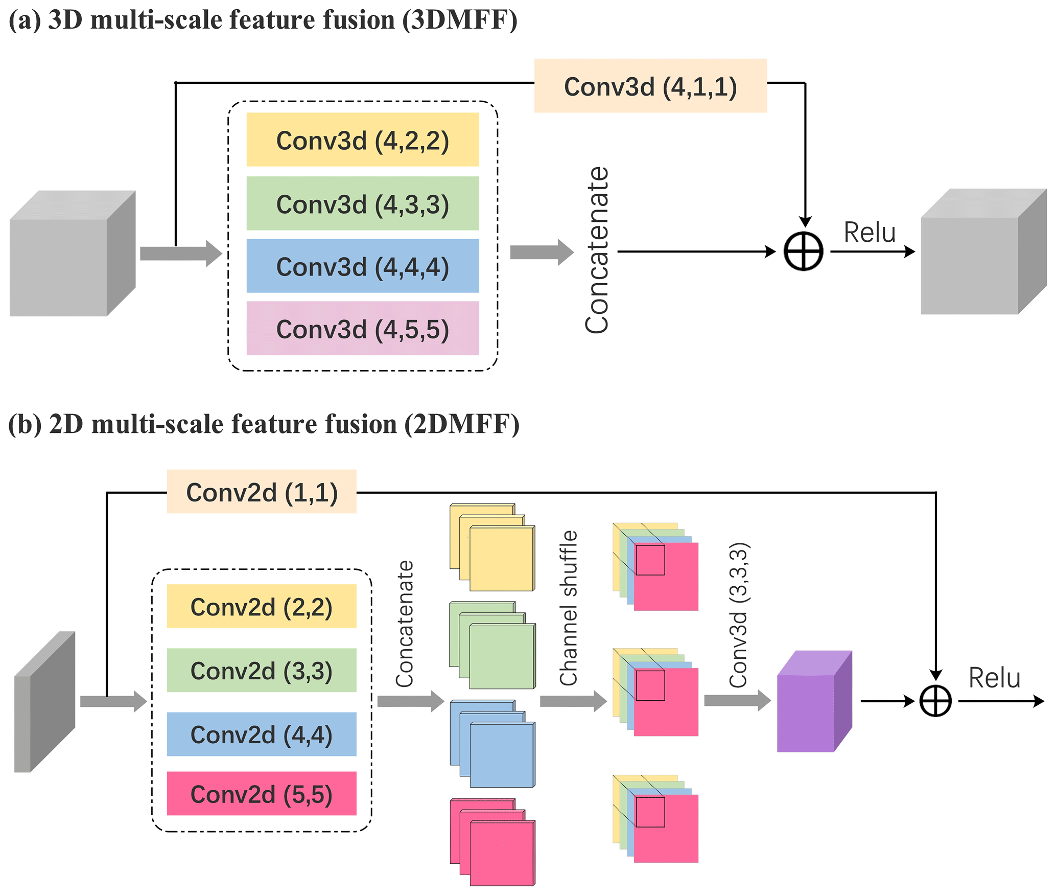
Figure 2 Panel (a) shows the 3D multi-scale feature fusion (3DMFF) and (b) the 2D multi-scale feature fusion (2DMFF).

Consequently, as compared with the conventional single-feature module, the MFF modules use different receptive fields to enhance feature interaction and increase the number of network routes. This enables the MFF modules to fully extract feature information that was previously lost due to fewer network routes. Additionally, the MFF modules introduce channel sorting and spatial–temporal convolutions to address the issue of information redundancy.

2.3 Framework of the nowcasting model based on MFF

Here is a detailed description of the precipitation nowcasting model framework (Fig. 3) that we developed. The model is trained using 60 min radar echo maps, with an input size of $(\mathrm{1},\mathrm{10},\mathrm{880},\mathrm{1024})$ grid, and produces nowcasting outputs of 180 min, with a size of $(\mathrm{1},\mathrm{30},\mathrm{880},\mathrm{1024})$ grid. The model has two main components: the encoding and decoding networks. The encoding network uses multiple 3DMFF modules to extract features and compress information, while the decoding network involves feature restoration and up-sampling using 3D transpose convolutions and 2DMFF modules. The 3D transpose convolutions generate a tensor (see P in Fig. 3) that acts as the probability matrix, retaining the intensity information of radar echo for predicting various precipitation systems such as light rain, moderate rain, and heavy rain. To restore the decoding network's features to the input's features, we perform two Hadamard product operations. The first operation multiplies the output features of the 2DMFF by the probability matrix (see m⊙P in Fig. 3), while the second operation multiplies the output features of the 3D transpose convolutions by 1−P (see $(\mathrm{1}-P)\odot f_{\mathrm{1}}$ in Fig. 3). Since the outputs from 3D transpose convolutions lack edge information, we concatenate them with the outputs from the 2DMFF modules to reduce information loss. Finally, we apply a 3D convolution operation to adjust the channel of the product outputs and generate the precipitation nowcasting results.

By drawing lessons from “MetNet” (Sønderby et al., 2020), let us suppose the target weather condition is y and the input condition is x; thus,

$$\begin{array}{}\text{(1)}& p\left(y\right|x)={\mathrm{DNN}}_{\mathit{\theta }}(x),\end{array}$$

where p(y|x) is a conditional probability over the output target y given the input x, and DNN_θ(x) is a deep neural network with parameter θ. The model used in this case introduces uncertainties because it calculates the probability distribution over possible outcomes and does not provide a deterministic output. In most cases, the radar echo reflectivity is a continuous variable, and we need to discretize the variable into a series of intervals to approximate the probability density function of the variable. By using a discrete probability model, we can reduce uncertainties. Therefore, the combination of discrete probability and radar echo reflectivity can significantly reduce uncertainties of extrapolative radar echo. Here, we use a mechanism of discrete probability as follows:

$$\begin{array}{}\text{(2)}& y^{\left[\mathit{\tau }\right]}=\sum _{i=\mathrm{1}}^c{p}_i^{\left[\mathit{\tau }\right]}\left(y^{\left[\mathit{\tau }\right]}|x\right)\cdot x_i,\end{array}$$

where y^[τ] is the output at a given time τ, x is the input condition, c is the number of channels, and $p_i^{\left[\mathit{\tau }\right]}\left(y^{\left[\mathit{\tau }\right]}\right|x)$ is a conditional probability. Equation (2) shows the information of multiple channels at time τ. Here, each channel has its own probability value, which is used to extract better features. The conditional probability $p_i^{\left[\mathit{\tau }\right]}$ is multiplied by related channel information x_i and their sum is calculated over all channels to obtain more realistic radar echo reflectivities. The mechanism of discrete probability is used by both m⊙P and $(\mathrm{1}-P)\odot f_{\mathrm{1}}$ (see Fig. 3).

Figure 3 The framework of the nowcasting model based on multi-scale feature fusion (MFF).

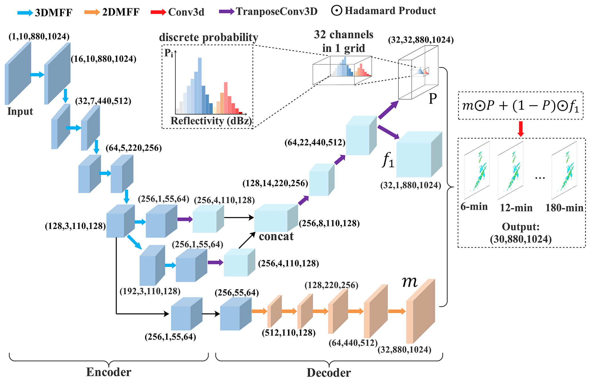
Overall, the nowcasting model has a deep and hierarchical encoding–decoding backbone that helps to extract essential features from inputs. It also has several plug-and-play modules suitable for excavating context information, reducing background noise and identifying texture features. This makes the model effective in investigating the movement vector features of precipitation systems such as shape, movement direction, and moving speed. The model also uses the mechanism of discrete probability to reduce uncertainties and forecast errors, which helps to postpone the declining rate of strong-intensity echoes to some extent. Therefore, the model can produce heavy rains with longer lead times.

2.4 Comparative models

To provide a thorough comparison, here we also present three radar echo extrapolation models.

2.4.1 Optical flow

The problem of radar echo extrapolation can be seen as detecting moving objects, which involves separating targets from a continuous sequence of images. Gibson (1979) introduced the concept of optical flow (OF), which characterizes the instantaneous velocity of pixel motion of a space object in an imaging plane. The OF method employs the variation of a pixel of the image sequence in the time domain and the correlation between two adjacent frames to investigate the movement information of objects between consecutive frames. Essentially, the transient variation of a pixel on a certain coordinate of the 2D imaging plane is defined as an optical flow vector. The OF method relies on two basic assumptions: grayscale invariance and the small movement of pixels between consecutive frames.

Letting $I(x,y,t)$ be the grayscale value of the pixel at position (x,y) and time t, it moves (dx,dy) units of distances using dt units of time. Based on the grayscale invariant hypothesis, the grayscale value remains unchanged between two adjacent times, so the following equation holds:

$$\begin{array}{}\text{(3)}& I(x,y,t)=I(x+\mathrm{d}x,y+\mathrm{d}y,t+\mathrm{d}t).\end{array}$$

Using Taylor expansion, the right term of Eq. (3) becomes

$$\begin{array}{}\text{(4)}& I(x,y,t)=I(x,y,t)+{\displaystyle \frac{\partial I}{\partial x}}\mathrm{d}x+{\displaystyle \frac{\partial I}{\partial y}}\mathrm{d}y+{\displaystyle \frac{\partial I}{\partial t}}\mathrm{d}t+\mathit{ϵ},\end{array}$$

where ϵ represents the infinitesimal of the second order which is negligible. Then substitute Eq. (4) into Eq. (3) and divide by dt. Thus, we have

$$\begin{array}{}\text{(5)}& {\displaystyle \frac{\partial I}{\partial x}}{\displaystyle \frac{\partial x}{\partial t}}+{\displaystyle \frac{\partial I}{\partial y}}{\displaystyle \frac{\partial y}{\partial t}}+{\displaystyle \frac{\partial I}{\partial t}}=\mathrm{0}.\end{array}$$

Suppose $u=\mathrm{d}x/\mathrm{d}y$ and $v=\mathrm{d}y/\mathrm{d}y$ are two velocity vectors of optical flow along the x axis and the y axis, respectively. Let $I_x=\frac{\partial I}{\partial x}$, $I_y=\frac{\partial I}{\partial y}$, and $I_t=\frac{\partial I}{\partial t}$ be the partial derivatives of the grayscale of pixels along the x axis, the y axis, and the t axis, respectively. Thus, Eq. (5) turns into

$$\begin{array}{}\text{(6)}& I_{x}u+I_{y}v+I_t=\mathrm{0},\end{array}$$

where I_x, I_y, and I_t can be calculated from the original image data, while (u,v) are two unknown vectors. Because Eq. (6) is a constraint equation but has two unknown variables, it is necessary to add other constraint conditions to calculate (u,v). Currently, there are two common algorithms used to solve this problem: global optical flow (Horn and Schunck, 1981) and local optical flow (Lucas and Kanade, 1981), detailed mathematical derivations of the two algorithms which we do not expatiate here.

2.4.2 UNet

The second comparative model is U-Net. Unlike the MFF model, the UNet model uses general 2D convolution instead of the “MFF module”. It consists of three main parts. The first part, called the encoder module, is a backbone network that performs down-sampling and feature extraction. It is composed of several convolution layers and max-pooling layers. The second part, called the decoder module, uses several up-convolution layers and convolution layers to conduct up-sampling and strengthen feature extraction. This allows for effective feature fusion based on the output features from the first part. Finally, the third part is a prediction module that is used for a specific task, such as regression and segmentation. Additionally, to ensure that the down-sampling feature's size matches the up-sampling feature's size, and to further preserve more original information, the “feature copying and cropping” operation is also required.

2.4.3 Time series residual convolution

The third comparative model is time series residual convolution (TSRC) proposed in our previous study (Huang et al., 2023). The model compensates for the current local radar echo features with previous features during convolution processes on a spatial scale. It also incorporates “time series convolution” to minimize dependencies on spatial–temporal scales, resulting in the preservation of more contextual information and fewer uncertain features in the hierarchical architecture. The model has shown excellent performance in handling the smoothing effect of the precipitation field and the degenerate effect of the echo intensity. (For detailed mathematical derivations of the TSRC model, please refer to our previous study.)

2.5 Evaluation metrics

We utilize five metrics to assess the forecast accuracy of three models: probability of detection (POD), false alarm rate (FAR), mean absolute error (MAE), radially averaged power spectral (RAPS), and structural similarity index (SSIM). Their mathematical equations are as follows:

$$\begin{array}{}\text{(7)}& {\displaystyle }\mathrm{POD}={\displaystyle \frac{\text{successful forecast}}{\text{successful forecast}+\text{missing forecast}}}\text{(8)}& {\displaystyle }\mathrm{FAR}={\displaystyle \frac{\text{null forecast}}{\text{successful forecast}+\text{null forecast}}}.\end{array}$$

In practical precipitation tasks, it is common to encounter successful forecasts, missing forecasts, and null forecasts, which are determined by comparing the ground true value (GTV), forecast value (FV), and threshold value (TV). Here, the threshold of 20 dBz is used to represent reflectivity values greater than 20 dBz (referred to as “∼20 dBz”). Similarly, “∼30” and “∼40 dBz” can be abbreviated. This study adopts three thresholds (20, 30, and 40 dBz). To determine the occurrence of successful forecast events, mark one if GTV ≥ TV and FV ≥ TV. For missing forecast events, mark one if GTV ≥ TV and FV < TV. For null forecast events, mark one if GTV < TV and FV ≥ TV. The performance of growth and dissipation forecasting tasks can be intuitively described by both POD and FAR:

$$\begin{array}{}\text{(9)}& \mathrm{MAE}={\displaystyle \frac{\mathrm{1}}{n}}\sum _{i=\mathrm{1}}^n|Y_i^{\mathrm{g}}-Y_i^{\mathrm{f}}|,\end{array}$$

where $Y_i^{\mathrm{g}}$ and $Y_i^{\mathrm{f}}$ are the ground truth value and forecast value in the ith pixel of the related echo image and n is the total number of pixels. This metric describes the performance of each forecast model at different precipitation intensity levels.

In this study, the radar echo's grayscale is considered a signal. The power spectrum describes the different frequency components' magnitudes of a 2D image signal. Therefore, we use the Fourier transform to convert it from the spatial domain to the frequency domain (Braga et al., 2014). Different frequency components in the power spectra are located at varying distances and directions from the base point on the frequency plane. High-frequency components are farther from the base point, and different directions indicate different orientations of the data features. To investigate the smoothing effect of forecast radar echo maps and discuss the forecast skill on local convection, we use RAPS (Sinclair and Pegram, 2005; Ruzanski and Chandrasekar, 2011). Here are the mathematical derivations of RAPS in detail. First, we perform a 2D Fourier transform on a 2D input image:

$$\begin{array}{}\text{(10)}& F(u,v)=\mathcal{F}\mathit{\left\{}f\right(x,y\left)\mathit{\right\}},\end{array}$$

where F(u,v) is the representation of complex domain after Fourier transform, ℱ is the Fourier operator, and f(x,y) is the input image. Next, we calculate the power spectral P and radial coordinate r in the frequency domain:

$$\begin{array}{}\text{(11)}& P(u,v)=\left|F\right(u,v){|}^{\mathrm{2}},r(u,v)=\sqrt{u^{\mathrm{2}}+v^{\mathrm{2}}}.\end{array}$$

Last, the power spectra are grouped according to the radial coordinate of frequency; subsequently, we take the average. For each radius r_k, its corresponding radially averaged power spectral P_k is

$$\begin{array}{}\text{(12)}& P_k={\displaystyle \frac{\mathrm{1}}{N_k}}\sum _{i}P(u_i,v_i),\end{array}$$

where $r(u_i,v_i)\approx r_k$, and N_k is the number of frequency points falling within the radius of r_k.

In addition, we calculate the SSIM (Wang et al., 2004) to examine the similarity of precipitation fields between ground true and forecasting radar echo maps:

$$\begin{array}{}\text{(13)}& \mathrm{SSIM}={\displaystyle \frac{(\mathrm{2}{\mathit{\mu }}_{\mathrm{g}}{\mathit{\mu }}_{\mathrm{f}}+c_{\mathrm{1}})(\mathrm{2}{\mathit{\sigma }}_{\mathrm{gf}}+c_{\mathrm{2}})}{({\mathit{\mu }}_{\mathrm{g}}^{\mathrm{2}}+{\mathit{\mu }}_{\mathrm{f}}^{\mathrm{2}}+c_{\mathrm{1}})({\mathit{\sigma }}_{\mathrm{g}}^{\mathrm{2}}+{\mathit{\sigma }}_{\mathrm{f}}^{\mathrm{2}}+c_{\mathrm{2}})}},\end{array}$$

where μ_g and μ_f are the means of ground truth and forecasting radar echo map, σ_g and σ_f are the related standard deviations, and σ_gf is the covariance, respectively. c₁ and c₂ are two constants. These metrics reflect the movement of precipitation fields between the ground truth and forecasting radar echo map.

3 Results

3.1 Overall forecast performances on testing data

We use 4 years of data (2018–2021) for model training and 1 year of data from 2022 for model testing. In Fig. 4, we show the four evaluation metrics, i.e., POD, FAR, MAE, and SSIM, in three reflectivity intervals of ∼20, ∼30, and ∼40 dBz. Overall, we observed that POD in the four models consistently decreases with increased forecast lead time for all reflectivity intervals, while FAR increases. The rankings of POD (or FAR) are quite different for the three reflectivity intervals. In the ∼20 dBz reflectivity interval, MFF ranks the highest in POD during the entire forecast period, remaining stable ranging from 0.6 to 0.8, which is almost twice that of TSRC, OF, and UNet after the 2 h lead time. However, MFF and TSRC have nearly equal FAR, which is roughly half of that of OF and UNet. In the ∼30 dBz reflectivity interval, TSRC ranks highest in POD, followed by MFF. Coincidentally, TSRC also ranks highest in FAR before the 1 h forecast time, while both MFF and TSRC obtain relatively low FAR compared with that of OF and UNet. In the ∼40 dBz reflectivity interval, POD in TSRC is ahead of the other three models, especially before the 1 h lead time, and it degrades into that of MFF at the longer lead time. POD in both OF and UNet remains lower than 0.2 during the entire forecast period and nearly declines to 0 after the 2 h lead time; MFF reports the lowest FAR during the entire forecast period. While the value of FAR climbs from about 0.1 to 0.9, TSRC has a relatively stable FAR, while the value of FAR is higher than 0.5 during the entire forecast period. FAR in OF and UNet rapidly increases from about 0.1 to 0.8 in the first 90 min. FAR in all models is greater than 0.8.

Although MFF produces relatively low POD in high reflectivity (∼30 and ∼40 dBz) intervals compared with TSRC, it obtains relatively low FAR at the same time. From the definition of POD/FAR, it can be understood that both more “successful forecasts” and more “null forecasts” occur in TSRC, while fewer “successful forecast” events and fewer “null forecast” events occur in MFF compared with TSRC for high reflectivity intervals. If we take POD =0.6 as a dividing point, it is clear that MFF yields ”successful forecast” events for the whole forecast period in ∼20 dBz reflectivity, while TSRC, OF, and UNet gain “successful forecast” events only before 60, 24, and 36 min, respectively. Similarly, if we take FAR =0.5 as a dividing point in ∼40 dBz reflectivity, it can be found that MFF, OF, and UNet report FAR <0.5 only before 2 h, 30 min, and 30 min, respectively, suggesting that at least the three models can avoid half of the “null forecast” events before 2 h, 30 min, and 30 min, respectively. However, TSRC is unavoidable in producing “null forecast” events for the whole forecast period in ∼40 dBz reflectivity.

We also analyze the mean absolute error and structural similarity index metric between the nowcasting and ground truth. The MAE gradually increases with the forecast time for all models. Out of the three models, MFF has the smallest MAE (around 15 dBz), which is better than both TSRC and UNet by approximately 2 dBz reflectivity after 90 min. On the other hand, OF has the highest MAE, particularly in long forecast times. This indicates that MFF reproduces the precipitation intensity with relatively less overestimation or underestimation compared with the other models, while OF shows little capacity to do so, especially in a long forecast time. In terms of SSIM, it can be found that MFF performs well and maintains an upward trend, while OF remains consistent throughout the forecast time. However, TSRC and UNet show a downward trend, especially after 90 min. This indicates that MFF is capable of capturing the shapes of precipitation fields with relatively high similarity, and its forecast performance improves with forecast times.

Understandably, the MFF model can identify movement vectors of precipitation systems and reduce uncertainties in high reflectivity intervals. By using the mechanism of discrete probability, the model is particularly effective for high-intensity precipitation systems even at longer forecast times. However, the TSRC model may struggle to replenish the information on precipitation intensity, leading to overestimation for the entire forecast period and producing more “null forecasts” events. On the other hand, the OF model produces precipitation fields based on the grayscale invariant and the slight movement of the precipitation system, making it difficult to detect fast changes in precipitation fields, especially in longer forecast times. Additionally, it tends to overestimate or underestimate high-intensity precipitations. Lastly, the UNet model only performs feature extractions on the spatial scale, leading to information loss and an inability to detect fast changes in precipitation fields on the temporal scale and high-intensity precipitations. Consequently, it has poor performance in nowcasting throughout the forecast period.

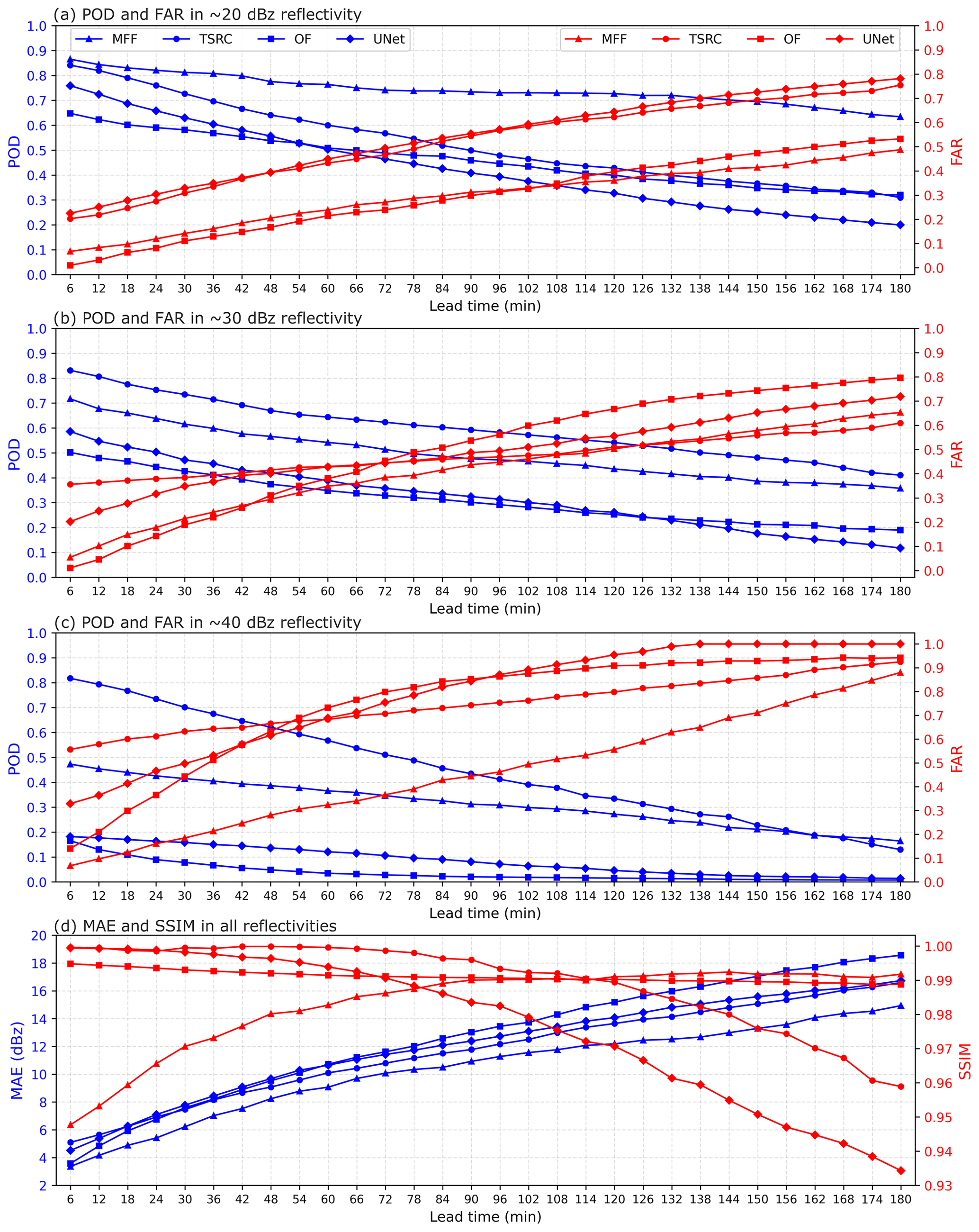
Figure 4 The forecast results in terms of four evaluation metrics on testing data for the whole year of 2022.

3.2 Results of case study

Here we present forecast results for two real precipitation cases (see Fig. 5) to better understand the performance of the four models.

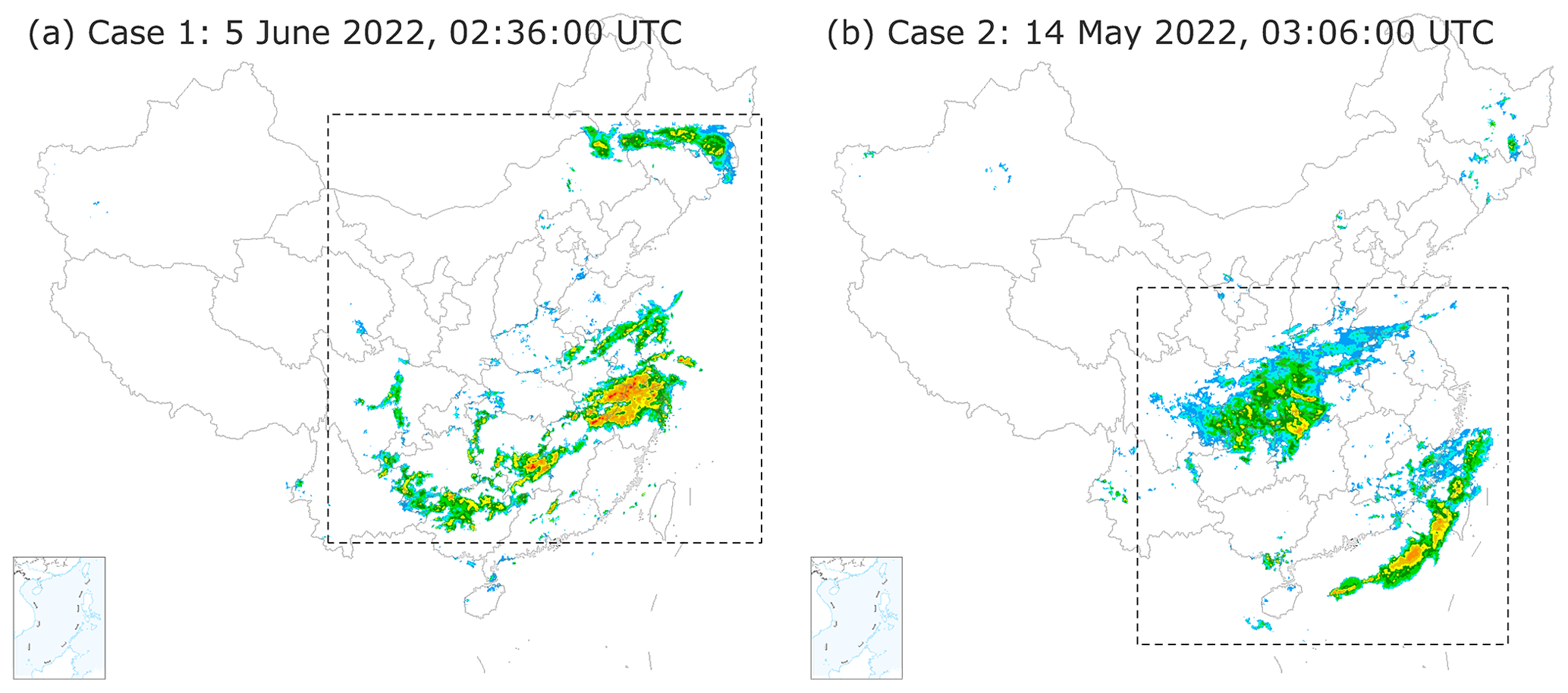
Figure 5 Overhead depiction of two precipitation cases in China, the left lower corner shows the South China Sea. Publisher's remark: please note that the above figure contains disputed territories.

3.2.1 Case 1

The first case is a large-scale precipitation process over China on 5 June 2022, 02:36:00 UTC (Fig. 5a). It contains the north part over northeastern China affected by a cold vortex and the south part (also known as “dragon-boat rain”) over southern China affected by warm, humid air. Figure 6 presents the forecast results of this case. In the ground truth, the whole precipitation area keeps a sluggish enlarging trend with the increased lead time, but the precipitation area of the high-intensity (e.g., greater than 35 dBz) echoes narrows gradually. As an important finding, MFF shows the best forecast performances since it can predict high-intensity (e.g., greater than 45 dBz) echoes even at the longest lead time (T+180 min). Comparatively, TSRC and UNet produce these echoes only at the short-range forecast time and miss them at the longest lead time. In terms of the precipitation field, both MFF and TSRC roughly capture the precipitation area, especially for low-intensity (e.g., less than 30 dBz) echoes at short-range lead times. OF draws an obvious dragged trajectory of the precipitation field in longer lead times, indicating the model simply creates precipitation fields with symbolic replications from the first frame to the last frame (T+180 min) at a horizontal scale and always misses the local changes of the precipitation system. UNet is difficult to grasp the whole precipitation field, not to mention the heavy precipitation system, and its precipitation field narrows gradually with the increasing lead time and finally disappears. The above analysis seems to be in accord with previous results that the high POD is reported in MFF and TSRC for low-intensity echoes (Fig. 4a), while there is relatively steady POD in OF and UNet for high-intensity echoes (Fig. 4b and c). Overall, MFF outperforms the other three models in predicting the precipitation field and the heavy precipitation.

On 5 June 2022 at 02:36:00 UTC, a large-scale precipitation process occurred over China, affecting northeastern China and southern China differently. The northeastern part was affected by a cold vortex, while the southern part experienced warm, humid air, also known as “dragon-boat rain”. In Fig. 5a, the forecast results of this case are presented, with the ground truth showing a sluggish enlargement of the whole precipitation area but a gradual narrowing of high-intensity echoes (greater than 35 dBz). An important finding is that MFF has the best forecast performances, predicting high-intensity echoes even at the longest lead time (T+180 min). In contrast, TSRC and UNet only produced these echoes at short-range forecast times and missed them at the longest lead time. In terms of the precipitation field, both MFF and TSRC roughly capture it, especially for low-intensity echoes (less than 30 dBz) at short-range lead times. OF draws an obvious dragged trajectory of the precipitation field in longer lead times, indicating the model simply creates precipitation fields with symbolic replications from the first frame to the last frame (T+180 min) at a horizontal scale, always missing the local changes of the precipitation system. It is definitely difficult for UNet to grasp the whole precipitation field, not to mention the heavy precipitation system, and its precipitation field narrows gradually with the increasing lead time and eventually disappears. The above analysis is in line with previous results that MFF and TSRC have high POD for low-intensity echoes (see Fig. 4a), while OF and UNet have relatively steady POD for high-intensity echoes (see Fig. 4b and c). Overall, MFF outperforms the other three models in predicting the precipitation field and heavy precipitation.

The RAPS metric is used to examine the smoothing and blurry precipitation fields. A lower power spectral indicates a smoother precipitation field. Conspicuously, OF enjoys a relatively high power spectral that is comparable to that of the ground truth for the entire wavelength range. At first glance, OF can accurately predict local convection activity and the evolution of the precipitation system. However, the model shifts the precipitation field from the first frame to the last, which results in poor forecast performance at longer lead times. The other three DL-based models (MFF, TSRC, and UNet) have relatively low power spectra, indicating that they introduce a smooth precipitation field to some extent. But they might describe the evolution of the precipitation system more reasonably. MFF has a low power spectral under 4 km wavelength, higher than that of TSRC and UNet. This difference becomes more significant at longer lead times, suggesting that the MFF model is better at describing local convection activity on a small scale. Overall, the MFF model does at least ease the smoothing effect.

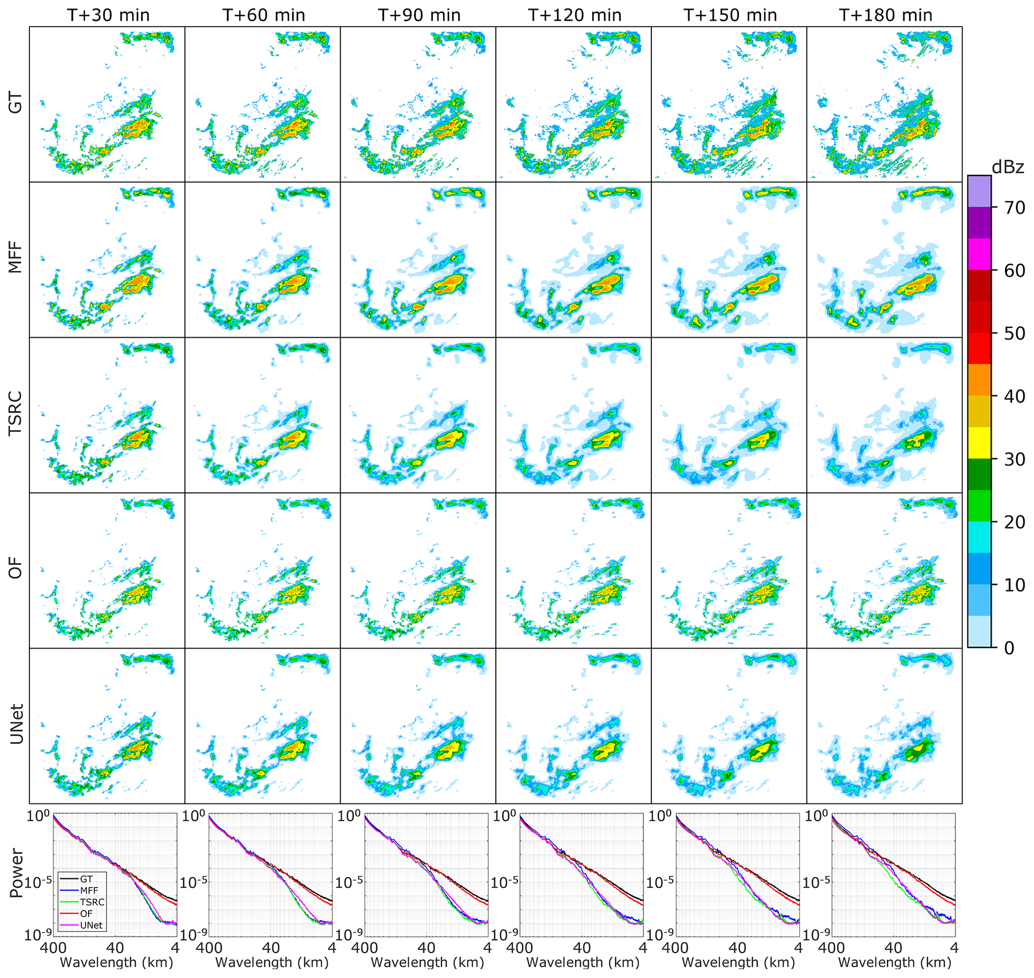
Figure 6 The precipitation maps of case 1 (5 June 2025, 02:36:00 UTC): ground truth (first row), multi-scale feature fusion (second row), time series residual convolution (third row), optical flow (fourth row), and UNet (fifth row). The sixth row shows the radially averaged power spectral density.

3.2.2 Case 2

On 15 May 2022 at 03:06:00 UTC, a significant precipitation event occurred in central China and offshore China (Fig. 5b). The event was influenced by the upper-level westerly trough, the southwest vortex, and the lower-level shear. The forecast results for this event are presented in Fig. 7, The precipitation area gradually expands, but the high-intensity area decreases with lead times. Both the MFF and TSRC models roughly follow the shape of the precipitation areas on land and sea and provide the evolutionary trend of the precipitation system. However, the OF model shifts the precipitation field from the first frame to the last frame, missing the evolutionary trend of the precipitation system, particularly for longer lead times. This confirms the model's poor ability to forecast precipitation over long ranges. The UNet model proved to be the most challenging to use in capturing the evolutionary trend of the precipitation system, as it reproduces the small precipitation field, which is the opposite of the ground truth. The four models show different forecasting performances in terms of echo intensity. MFF overestimates strong-intensity echoes (greater than 30 dBz), but it also increases the area of echoes at all lead times. TSRC cannot produce strong echo intensities after the 120 min lead time. OF can predict strong-intensity echoes at longer lead times, but the model's prediction is almost identical to the first frame, indicating a poor performance in predicting the evolution of strong-intensity echoes. Unfortunately, UNet shows the worst forecast performance since it underestimates these strong intensities at shorter lead times and cannot deduce these strong-intensity echoes at longer lead times.

The three DL-based models report relatively low power spectra before the 90 min lead time. OF obtains relatively high power spectra, which are almost equal to the ground truth at all lead times. This is because OF shifts the precipitation field using an extrapolative technique. It is noteworthy that the power spectral in MFF is slightly greater than that in TSRC and UNet at longer lead times, suggesting that the smoothing effect is further improved by MFF, making it more suitable for precipitation forecasting both on land and sea.

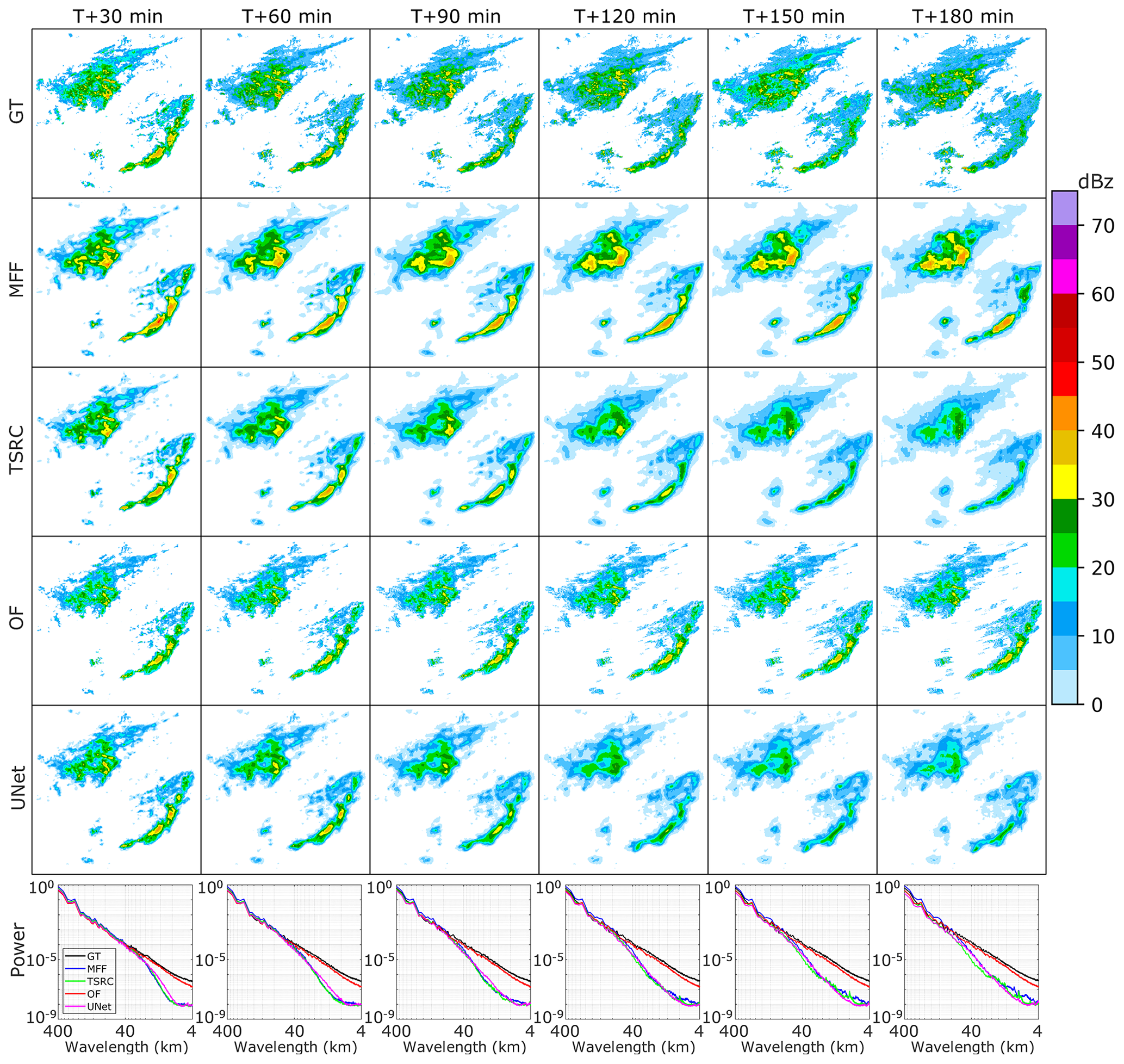
Figure 7 Same as in Fig. 6, but for the precipitation in case 2 (15 May 2022, 03:06:00 UTC).

3.3 Discussion

Here we summarize the advantages and disadvantages of the four models in precipitation nowcasting.

3.3.1 MFF

The purpose of MFF is to improve the accuracy of precipitation forecasting, particularly at longer lead times. Current DL-based models for precipitation forecasting are faced with two major challenges: the poor forecast skill when different precipitation systems with varying scales are present; and the low predictive accuracy when different precipitation targets, such as light rain, moderate rain, and heavy rain, are densely distributed in a certain area of interest and also introduce noises. From a qualitative perspective, MFF proposes a deep and hierarchical encoding–decoding architecture that can make full use of the receptive fields to efficiently detect different precipitation systems in multi-scales and predict various precipitation targets. This superiority is unable to be achieved by the traditional single-scale receptive fields. However, this architecture shows strong ability in feature extraction but might also account for the issue of information redundancy. Therefore, the model employs several techniques, such as channel shuffle, feature concatenation, and spatial–temporal convolution, to enhance the feature interaction ability among multi-scales and further ease information redundancy. These techniques do obtain considerable forecast performance in several evaluation metrics, including POD, FAR, MAE, and SSIM. Additionally, the model skillfully applies the mechanism of discrete probability, which mathematically allocates the probability information into each channel and can reduce uncertainties and forecast errors to the most extent. The results of the case study further prove that only this model can produce heavy precipitations such as those greater than 45 dBz reflectivity radar echoes even at the 3 h lead time. It is noteworthy that two tricky issues, namely the smoothing effect and cumulated error, are still inevitably reported in the model. However, these issues are not specific to MFF, as most DL-based models are also confronted. The principal reasons accounting for them include that the convolution strives to smooth multi-scale features in receptive fields to minimize fitting errors and that there are iterative discrepancies between the training processes and targets. Encouragingly, by introducing the MFF and the mechanism of discrete probability, at least our models have some improvements. This offers a lot of promise for handling practical tasks such as precipitation growth and dissipation, fast-moving precipitation systems, heavy precipitation, and local convection activity. In any event, MFF is a DL-based and data-driven radar extrapolative model without any consideration of physical constraints and atmospheric dynamics. Hopefully, the model can be further improved by adding multi-source data and combining ingenious DL architectures.

Furthermore, like other convolution-based DL models, the MFF model also requires highlighting the “inductive bias” to improve its generalization ability. Inductive bias can be thought of as a sort of “local prior”. In the case of image analysis, the inductive bias in the MFF model mainly consists of two aspects. The first aspect is “spatial locality”, which assumes that adjacent regions in a radar echo image always have relevant precipitation features. For example, the region of strong-intensity echoes is usually accompanied by the region of moderate-intensity echoes. However, this inductive bias may sometimes overestimate the precipitation intensity (see case 2 in Fig. 7). or enlarge the precipitation field, leading to accuracy issues. The other aspect is “translation equivariance”, which means that when the precipitation field in the input map is translated, the precipitation field is also translated due to the use of local connection and weight-sharing in the multi-scale convolution process. This feature does allow the MFF model to trace the moving precipitation system. Therefore, as a widely concerned weather phenomenon, extreme precipitations (e.g., 1-in-100-year rainfall events) may also be extrapolated and predicted by using inductive bias in the MFF model if both the training dataset and testing input provide precipitation events with very strong radar echoes. Conversely, it is also very challenging for the MFF model to tackle such a forecasting task.

3.3.2 TSRC

Essentially, TSRC is a reinforced “encoding–decoding” architecture that adds previous features to current feature planes on temporal scales during convolution processes. This allows more contextual information and fewer uncertain features to remain in deep networks. The model takes into account the correlation of radar echo features on a temporal scale, which theoretically reduces the problem of information loss and the degenerate effect intensity. However, the compensatory features in the architecture may lack specificity and carry noises, which causes the model to increase the precipitation intensities at the whole forecast lead times mindlessly. Although the model has relatively high POD, it has high FAR and MAE, particularly for heavy precipitations. The model increases the depth of the hierarchical architecture with different learnable parameters, excavates the dependencies of echo features on both temporal and spatial scales, and uses several techniques, such as feature concatenation, residual connection, and attention mechanism, to prevent the declining rate of intensity and the smoothing effect. The testing data show that the model has great advantages at real forecast tasks, such as low-intensity precipitation systems, and slow-change precipitation systems, especially for short lead times. However, the model lacks consideration of multi-scale features due to the fixed/unique receptive field on spatial scales. This leads to great difficulty in many real forecast tasks, such as local-convection activity, growth and dissipation, fast-moving precipitation systems, and rapid changes in the rainfall field. Therefore, it is speculated that the model can be further improved by implementing feature extraction on multi-spatial scales.

3.3.3 OF

The main principle behind OF is to observe the variation of pixels in a sequence of images in the time domain. By examining the correlation of two adjacent frames, the algorithm can detect the movement of objects. However, OF can only accurately forecast precipitation systems that have slow changes even at short lead times. The model relies on two fundamental hypotheses, namely the grayscale invariance and the tiny movement of pixels. The grayscale invariance feature renders the model challenging to deal with precipitation systems characterized by swift intensity fluctuations. For the tiny movement of pixels, it can hardly satisfy the forecast of a fast-moving precipitation system. Unlike the DL-based models, OF generates precipitation fields based on Lagrangian persistence and smooth motion, which also fail to recognize both local and multi-scale features of the precipitation system. This leads to poor forecasting ability at longer lead times, and the model often produces inaccurate results by merely shifting the precipitation fields. Although improved methods like the semi-Lagrangian method, which relies on the advection field, have been developed, they still struggle to explain the complex features of the precipitation system.

3.3.4 UNet

The UNet architecture involves three important steps, namely encoding, decoding, and skip connection. The encoding procedure uses multiple convolution layers for down-sampling and feature compression. This allows the contracting path to capture more context information. On the other hand, the decoding process applies several deconvolution layers for up-sampling and feature restoration. This allows the expanding path to locate different features. The skip connection part fuses the pixel-level features and semantic-level features to achieve feature segmentation and reduce information loss. While the bottom of the hierarchical architecture collects low-frequency information in the form of greater receptive fields, it fails to capture high-frequency information. As a result, when it comes to forecast tasks, the model may focus on those global (abstract or essential) features of precipitation systems but omit those exquisite changes in precipitation systems at spatial–temporal scales. Since radar echoes usually have variability at multiple scales, it is insufficient for UNet to capture complex features of the precipitation system. The results from the case study also confirm that the model has poor forecast skills in fast-moving precipitations, high-intensity precipitations, growth, and dissipation, as well as long-term forecasting. In summary, UNet has the worst forecast performance among the three DL-based models.

4 Conclusions

This study presents MFF, a deep learning model designed for large-scale precipitation nowcasting with a lead time of up to 3 h. The model aims to investigate the movement features of precipitation systems on multiple scales. To reduce uncertainties and forecast errors, we introduce the mechanism of discrete probability in the model. We compare our model with three existing radar echo extrapolative models, namely TSRC, OF, and UNet. The comprehensive analyses of testing data further prove the impressive forecast skills of MFF under four evaluation metrics: POD, FAR, MAE, and SSIM. MFF is the only extrapolative model that produces heavy precipitations even at the 3 h lead time, and the smoothing effect of the precipitation field is improved. From an early warning perspective, the model shows a promising application prospect.

It is well known that data always determine the upper limit of a machine learning model, while algorithms only attempt to approximate this limit. Regretfully, the current study only considers the radar echo data as the model inputs. Therefore, we highly recommend considering more meteorological variables, such as temperature, pressure, humidity, wind, and so on, as well as ground elevations, in future work. These data can come from various sources such as radar observations, satellite sounding, reanalysis, real-time observation, NWP downscaling, and so forth. We believe that these multi-source data can fortify some kind of physical or thermodynamic constraint for a pure data-driven extrapolative model. The smoothing effect remains a challenging task, and it is still reported as long as the convolution procedure is performed. Therefore, future work will focus on the structural adjustments of the network and the combinations with numerical models to further improve the forecast accuracy of heavy precipitations at longer lead times.