the Creative Commons Attribution 4.0 License.
the Creative Commons Attribution 4.0 License.
 | 22 Jan 2024
Exploring the ocean mesoscale at reduced computational cost with FESOM 2.5: efficient modeling strategies applied to the Southern Ocean
Thomas Rackow
Tido Semmler
Thomas Jung
Modeled projections of climate change typically do not include a well-resolved ocean mesoscale due to the high computational cost of running high-resolution models for long time periods. This challenge is addressed using efficiency-maximizing modeling strategies applied to 3 km simulations of the Southern Ocean in past, present, and future climates. The model setup exploits reduced-resolution spin-up and transient simulations to initialize a regionally refined, high-resolution ocean model during short time periods. The results are compared with satellite altimetry data and more traditional eddy-present simulations and evaluated based on their ability to reproduce observed mesoscale activity and to reveal a response to climate change distinct from natural variability. The high-resolution simulations reproduce the observed magnitude of Southern Ocean eddy kinetic energy (EKE) well, but differences remain in local magnitudes and the distribution of EKE. The coarser, eddy-permitting ensemble simulates a similar pattern of EKE but underrepresents observed levels by 55 %. At approximately 1 ∘C of warming, the high-resolution simulations produce no change in overall EKE, in contrast to full ensemble agreement regarding EKE rise within the eddy-permitting simulations. At approximately 4 ∘C of warming, both datasets produce consistent levels of EKE rise in relative terms, although not absolute magnitudes, as well as an increase in EKE variability. Simulated EKE rise is concentrated where flow interacts with bathymetric features in regions already known to be eddy-rich. Regional EKE change in the high-resolution simulations is consistent with changes seen in at least four of five eddy-permitting ensemble members at 1 ∘C of warming and all ensemble members at 4 ∘C. However, substantial noise would make these changes difficult to distinguish from natural variability without an ensemble.
- Article
(8957 KB) - Full-text XML
-
Supplement
(1529 KB) - BibTeX
- EndNote


Mesoscale activity in the Southern Ocean has been the subject of much research and interest in recent years due to the intensification of Southern Hemisphere westerlies (Marshall, 2003), the phenomena of eddy saturation and compensation (Munday et al., 2013; Bishop et al., 2016), and the potential for carbon sequestration in the face of ongoing anthropogenic emissions (Sallée et al., 2012; Landschützer et al., 2015; Frölicher et al., 2015). Satellite observations already reveal an intensification of eddy activity in the Antarctic Circumpolar Current (ACC), and changes are attributed primarily to wind stress (Marshall, 2003; Hogg et al., 2015; Martínez-Moreno et al., 2021). Modeling studies have been able to reproduce the observed changes, as well as project continued intensification throughout the 21st century (Beech et al., 2022), but the modeled results rely on only partially resolved eddy activity relative to observations, leaving open the possibility for new findings or greater clarity.
Advances in computational capabilities have enabled ocean modeling science to make great progress in overcoming the substantial computational burden of simulating the mesoscale. However, shortcomings remain, particularly in the Southern Ocean where the Rossby radius can be as small as 1 km, increasing the computational cost of resolving eddies (Hallberg, 2013). Even model resolutions that can generally be considered eddy-resolving are only eddy-permitting poleward of 50∘ if grid spacing does not vary in space (Hewitt et al., 2020). This highlights an efficiency challenge in simulating the mesoscale with traditional model grids; resolutions necessary to resolve high-latitude, small-radius eddies are both prohibitively expensive and unnecessary to resolve mesoscale eddies in the lower latitudes. Fortunately, a growing number of modeling alternatives to traditional grids now enable dynamic spatial allocation of resources (Danilov, 2013; Ringler et al., 2013; Danilov et al., 2017; Jungclaus et al., 2022), creating the opportunity to more efficiently resolve the mesoscale.
As resource allocation in high-resolution modeling becomes spatially flexible in the pursuit of more efficient configurations, the temporal component must also be scrutinized for efficiency. Traditional modeling approaches require long spin-up periods in order to equilibrate the deep ocean and reduce model drift (Irving et al., 2021). Although the impacts of drift are not negligible, they generally affect large-scale processes in the deep ocean; mesoscale processes that require high resolutions to simulate are typically fast to equilibrate and will appear relatively quickly wherever large-scale ocean conditions lead to their creation. Admittedly, one cannot entirely disentangle the two scales, as mesoscale activity does affect the position of fronts, stratification, and the paths of ocean circulation (Marshall et al., 2002; Marzocchi et al., 2015; Chassignet and Xu, 2017). Yet, with equilibration times for the deep ocean on the scale of thousands of years (Irving et al., 2021), the possibility, and ultimately necessity, to reduce the resolution of spin-up runs relative to production runs must be investigated.
Advancing the concept of dynamic temporal allocation of resources further, the traditional transient climate change simulation also represents an efficiency bottleneck for some applications; by modifying the climate continuously in time, each year of a transient simulation is effectively a single realization of a global mean climatic state that varies from the following and preceding years by only a fraction of a degree. For some applications, like hindcasts of real events or trend analysis, this approach may be desirable, but for assessing the impacts of climate change with limited resources and a low signal-to-noise ratio, a larger sample of realizations for a consistent climatic state may be more suitable.
Aside from oceanic concerns, the atmosphere can have substantial impacts on mesoscale activity in climate models. Most simply, with a coupled atmosphere, absolute surface winds will react to ocean eddy activity, whereas atmospheric forcing will not, resulting in more eddy killing by wind stress (Renault et al., 2016). Additionally, an atmosphere coupled to a high-resolution ocean must be of similarly high resolution for certain mesoscale interactions to be resolved (Byrne et al., 2016). Ultimately, the modeled atmosphere further escalates the already exponential cost of increasing ocean resolution by requiring more computational resources in order for the benefits of the resolved mesoscale to fully transfer to the broader climate.
To address the computational inefficiencies outlined above, a novel simulation configuration is proposed, combining several experimental modeling approaches. Simulations will exploit the multi-resolution Finite volumE Sea-ice Ocean Model (FESOM) (Danilov et al., 2017) employing a high-resolution unstructured mesh that concentrates computational resources on the Southern Ocean while maintaining grid resolution in the remainder of the global ocean that can still be considered high resolution, as in, for example, HighResMIP (Haarsma et al., 2016). The multi-resolution strategy overcomes the efficiency challenges of resolving high-latitude eddies without needlessly increasing tropical resolutions, as well as limiting the focus and computational requirements to one hemisphere. The high-resolution simulations will make use of a spin-up simulation on a medium-resolution, eddy-permitting mesh to avoid the computational burden of allowing an eddy-resolving ocean to equilibrate deep, slow-changing processes. The eddy-permitting mesh will also be used to simulate the transient periods between shorter, high-resolution time slices, increasing the signal-to-noise ratio of the results by separating the production data further in time and the progression of anthropogenic climate change. Finally, the ocean model will be forced with atmospheric data from existing coupled simulations (Semmler et al., 2020). Although this will not facilitate mesoscale atmosphere–ocean interaction, the simulation will reflect the climatic development of an eddy-permitting simulation of the future atmosphere without the additional computational requirements.
The Southern Ocean is one of the world's hotspots for mesoscale activity and a region where substantial change is anticipated in the context of anthropogenic climate change (Beech et al., 2022). Simultaneously, the high latitude of the region makes eddy-resolving model simulations computationally demanding and observational data relatively scarce (Auger et al., 2023; Hallberg, 2013). Yet, as the climate changes, the importance of the Southern Ocean grows as a heat and carbon sink, an ecosystem, and a medium for feedback between the atmosphere and ocean (Byrne et al., 2016; Frölicher et al., 2015). Thus, the study of the Southern Ocean demands innovation in the modeling field to produce high-resolution simulations at reduced computational cost. This study maximizes grid resolution relative to computational cost using an unstructured, multi-resolution grid, a medium-resolution spin-up simulation, and atmospheric forcing from lower-resolution coupled simulations in order to focus resources as much as possible on resolving mesoscale activity in the study region. The resulting simulations enable an exploratory analysis of the past, present, and future of the Southern Ocean with a fully resolved mesoscale. Simulations with this cost-efficient, high-resolution configuration are presented in comparison to a comprehensive ensemble of eddy-permitting simulations to assess the performance of the efficiency-focused approach in reproducing mesoscale activity and its response to climate change.
2.1 Experimental setup
This analysis contrasts a subset of simulations from AWI-CM-1-1-MR's contribution to the sixth phase of the Coupled Model Intercomparison Project (CMIP6; Semmler et al., 2020) (hereafter referred to as the AWI-CM-1 ensemble), with single-member standalone ocean simulations using an updated version of FESOM (FESOM 2.5) and a mesh substantially refined to a resolution surpassing 3 km in the Southern Ocean (hereafter referred to as the SO3 simulations) (Supplement Fig. S1). Observations of ocean surface velocity derived from satellite altimetry data are also used to evaluate model performance for both modeled datasets during the period of overlap with the altimetry record. The AWI-CM-1 simulations consist of the five-member ensemble of historical simulations and the five-member ensemble of climate change projections under shared socioeconomic pathway (SSP) 3-7.0 which were performed by AWI-CM-1-1-MR in CMIP6 (Semmler et al., 2020). These are state-of-the-art CMIP6 experiments and benefit from the multiple ensemble members and long spin-up times that CMIP simulations typically boast. However, while the AWI-CM-1 ensemble reproduces eddy activity remarkably well within the context of CMIP6 (Beech et al., 2022), high-resolution ocean modeling now far surpasses even the highest ocean resolutions in the CMIP6 ensemble. Conversely, the SO3 simulations push the limits of ocean resolution but rely on several measures for maximizing computational efficiency that may impact the robustness of the simulations. Details on the experimental setup for CMIP6 and ScenarioMIP are widely available (Eyring et al., 2016; O'Neill et al., 2016), and information more specific to AWI-CM-1-1-MR's contribution has been published previously (Semmler et al., 2020). The following sections will outline the details of the SO3 simulations.
To produce initial conditions for the high-resolution model simulations on the SO3 mesh, a medium-resolution, eddy-permitting, ocean-only transient simulation was first run from 1851 to 2100 using the same ocean mesh employed by AWI-CM-1-1-MR in CMIP6 (Semmler et al., 2020). This mesh has been shown to effectively reproduce eddy activity in active regions while maintaining a computational cost comparable to a traditional model (Beech et al., 2022). The transient simulation was initialized with conditions for ocean temperature and salinity, as well as sea ice concentration, thickness, and snow cover taken from the end of the first year (1850) and first ensemble member (r1i1p1f1) of AWI-CM-1-1-MR's historical simulations in CMIP6 (Semmler et al., 2018, 2020, 2022a, b). In this way, the model undergoes a semi-cold start in which ocean conditions are not exact continuations of the previous coupled simulation but should be far closer to equilibrium than a true cold start initialization. The eddy-permitting transient simulation was forced using atmospheric data from the same ensemble member of the historical CMIP6 simulations until 2014 (Semmler et al., 2022a) and thereafter using the first ensemble member of AWI-CM-1-1-MR's ScenarioMIP simulations for SSP 3-7.0 (Eyring et al., 2016; O'Neill et al., 2017; Semmler et al., 2022b). This approach to forcing takes advantage of a coupled simulation, CMIP6, to produce a forcing dataset of better temporal and spatial coverage than the observational record and which maintains a realistic transient climate throughout anthropogenic impacts during the 21st century.
In the years 1950, 2015, and 2090, FESOM is reinitialized with the high-resolution ocean grid, SO3 (Fig. S1), using the same semi-cold start approach and forcing dataset that were implemented for the eddy-permitting transient simulation described previously. These years were chosen to represent a historical period, beginning in 1950, when the effects of climate change on EKE should be small or none (Beech et al., 2022); a near-present period, beginning in 2015, in which the simulations will overlap with satellite altimetry data; and a projected period, beginning in 2090, which should include a strong climate change signal. The latter two simulated periods represent 1.07 and 3.74 ∘C of warming, respectively, in the first ensemble member of the AWI-CM-1 ensemble defined as a rise in the 21-year running mean of global mean 2 m air temperatures. Warming of the ensemble mean is similar: 1.08 and 3.76 ∘C, respectively, and warming is henceforth approximated as 1 and 4 ∘C in Fig. 4 and the text. Initial conditions for these shorter time-slice simulations are taken from the end of the previous year of the eddy-permitting transient simulation. The high-resolution simulations are each integrated for 6 years with the first year ignored as a true spin-up, leaving 5 years of data for each time period. The high-resolution grid is, in truth, a regionally refined mesh in which a 25 km global resolution is refined to approximately 2.5 km, following Danilov (2022), primarily south of 40∘ S, but with other pertinent regions, such as the Agulhas Current and several narrow straits, also refined. In this way, the model is able to simultaneously achieve eddy-rich conditions in the Southern Ocean and many of the nearby active regions, as well as a global resolution that would still be considered high in the context of CMIP6 (Hallberg, 2013; Hewitt et al., 2020). While model drift may be a concern with such a short true spin-up period, this should affect each of the high-resolution time slices similarly and to a limited extent due to their short integration lengths. Thus, the differences between the high-resolution ocean simulations should primarily reflect anthropogenic climate impacts simulated during the eddy-permitting transient run and present in the forcing dataset.
2.2 Model configuration
The Finite volume Sea-ice Ocean Model version 2.5 is a post-CMIP6 era model, having been refactored to a finite-volume configuration from the finite-element version (FESOM 1.4; Wang et al., 2014) employed in CMIP6 and transitioned to arbitrary Lagrangian–Eulerian vertical coordinates, among other improvements (Danilov et al., 2017; Scholz et al., 2019, 2022). FESOM's most distinguishing feature among mature ocean models is the unstructured horizontal grid that exploits triangular grid cells which can smoothly vary in size to change the horizontal grid resolution in space. In these simulations, full free surface, or z*, vertical coordinates were used, allowing the vertical model layer thicknesses to change in time. Gent–McWilliams eddy parameterization (Gent and McWilliams, 1990) is scaled with resolution according to Ferrari et al. (2010), and vertical mixing is simulated by a k-profile parameterization scheme (Large et al., 1994).
The SO3 mesh consists of over 22 million surface elements (triangle faces) or 11 million surface nodes (triangle vertices) and 70 vertical layers. The simulations produce about 1.1 terabytes of data per simulated year of 3D daily data stored on nodes. For reference, the medium-resolution mesh used in the AWI-CM-1 ensemble is 1.6 million surface elements or 0.83 million surface nodes and 46 vertical layers and produces approximately 56 GB per simulated year of 3D daily data stored on nodes. The model was run on 8192 CPU cores with a typical throughput of approximately 0.65 simulated years per day, consuming approximately 5.5 million CPU hours in total despite the various cost-saving modeling approaches. It should be noted, however, that the throughput in high-resolution production simulations like this is highly dependent on the volume and choice of data being saved. The simulations and following analyses were performed using the high-performance computing system, Levante, at the German Climate Computing Center (DKRZ).
The ocean model is forced by several atmospheric variables at a 6 h resolution, although one forcing variable, humidity, is interpolated monthly data. The forcing data are supplied to the model on the regular atmospheric grid used in the coupled setup during AWI-CM-1-1-MR's CMIP6 simulations (Semmler et al., 2018) and interpolated to the multi-resolution grid used in the respective simulations by FESOM. Runoff data are a monthly climatology, and dynamic ice sheet coupling is not included, meaning the freshwater influx from the Antarctic continent does not react to warming, which may impact certain processes, such as the timing and intensity of sea ice loss (Pauling et al., 2017; Bronselaer et al., 2018).
2.3 Modeled ocean velocity data
Geostrophic balance is an idealized approximation that does not match real ocean velocities for several reasons, including the presence of ageostrophic flow, such as Ekman transport, as well as assumptions made in the derivation of Eqs. (1) and (2). Specifically, geostrophic balance between the Coriolis effect and the pressure gradient is valid under the assumption that the curl of horizontal velocities or vorticity is small relative to the magnitude of overall flow. In models, this assumption is relatively close to reality in coarse-resolution simulations where geostrophic flow dominates, but on higher-resolution meshes, where submesoscale flows are well-resolved, these omitted terms become larger. Therefore, while using geostrophic velocities for both high-resolution and coarse-resolution modeled datasets would be methodologically consistent, the error introduced would be systemically larger for the finer-resolution dataset than the coarser. Therefore, we do not consider the use of geostrophic velocities for both modeled datasets in this analysis to bring the data into closer agreement. Rather, for the AWI-CM-1 dataset, where daily ocean velocities were not saved (Semmler et al., 2018), geostrophic velocities derived from sea surface height with Eqs. (1) and (2) are the best possible choice, and fortunately, as described earlier, the error introduced by the assumptions of geostrophic balance will be small. For the SO3 simulations, direct model output was saved and is preferred, particularly given the high resolution of the mesh.
The omission of Ekman transport, the primary source of ageostrophic oceanic flow from atmospheric influences, can be relatively well addressed in the SO3 dataset by selecting modeled velocities just below the Ekman layer. At depths of 25–30 m below sea level, the bulk of Ekman transport can be avoided (Price et al., 1987), while velocities should not substantially differ from those at the surface. What ageostrophic flow remains in the model output velocities should be primarily large scale and small relative to geostrophic flow in the high-energy regions of the ocean, including the ACC (Yu et al., 2021).
2.4 Altimetry data
An observational data product of gridded, daily geostrophic velocities derived from along-track satellite altimetry from crossover data is taken from the Data Unification and Altimeter Combination System (DUACS) (Taburet et al., 2019). The gridded product has a resolution of 0.25∘, although effective resolution at high latitudes may be much lower (Ballarotta et al., 2019). Recently, improved data have become available in the ice-covered regions of the Southern Ocean (Auger et al., 2022) but do not yet cover the full present-day simulated period (2016–2020) in this study. Absolute velocities from the gridded altimetry product were used to calculate anomalies and EKE using Eqs. (3) and (4) below for consistency with the modeled dataset.
2.5 EKE analysis
Velocity anomalies are defined by subtracting the multi-year monthly climatology of each respective 5-year period from daily velocities with Eq. (3).
where ui is the daily zonal velocity, ′ denotes an anomaly, and is a monthly mean. For meridional velocities (v) substitute u with v.
Eddy kinetic energy is calculated from ocean velocities according to Eq. (4).
where i denotes a daily value and ′ denotes an anomaly.
EKE was calculated on the native grid of each dataset and then interpolated to a 0.25∘ grid for all analyses. In Figs. 1 and 3, EKE was first calculated on a daily timescale and coarsened to 5 d means before analysis to reduce computational costs during post-processing. Area-integrated EKE (Figs. 1, 3) is calculated by summing the area-weighted EKE of each grid cell in the study region defined as the zonal band between 45 and 65∘ S. The Brazil–Malvinas confluence region between 57 and 29∘ E and northward of 40∘ S is removed to focus the study on a region with consistent physical drivers theorized to be responsible for the changes in eddy activity (Beech et al., 2022). As a precaution, each dataset was linearly detrended before analysis in Figs. 1 and 3 to avoid artificially increasing the range of the later distributions due to the accelerating climate change signal. Select statistical properties are reported in Supplement Tables S1–S3 to indicate deviations from normality (D'Agostino and Belanger, 1990; Fisher, 1997) and autocorrelation (Durbin and Watson, 1950). Rather than attempt to manipulate the data to meet certain statistical assumptions, complex statistical tests are avoided and the statistical properties reported can be used to interpret the EKE data in a physical sense. EKE anomalies (Fig. 1) were calculated by subtracting the 2016–2020 mean of area-integrated EKE from the 5 d mean values of each period. Normalized EKE was calculated by further dividing EKE anomalies by the standard deviation of EKE during the 2016–2020 period. In Fig. 4, ensemble agreement is determined by ordering the ΔEKE values within each grid cell from lowest to highest, plotting the positive values in increasing order from left to right and negative values in decreasing order from left to right.
3.1 Agreement with observations
During the 5-year period of overlap with observations, the SO3 simulation is a drastic improvement on the AWI-CM-1 ensemble in reproducing median observed EKE (Fig. 1a and c, note the different y axes); only a slight underrepresentation of EKE remains in the SO3 simulation, although the simulated distribution is somewhat distinct from observations. In comparison, the AWI-CM-1 ensemble, being effectively eddy-permitting in the Southern Ocean, underrepresents observations by approximately 55 % (Fig. 1a and c, note the different y axes). EKE in SO3 appears more variable than the observations considering its larger range (Fig. 1c, e), and in general, the modeled datasets display greater deviations from a normal distribution than the observations (Fig. 1a, b, c; Table S2). Nonetheless, relative to the AWI-CM-1 model bias and the magnitude of resolved EKE, the ensemble spread within the AWI-CM-1 dataset is small (Fig. 3), suggesting that a single ensemble member of 5 years' duration is sufficient to assess how well a model captures the magnitude of overall Southern Ocean EKE (Fig. 1c).
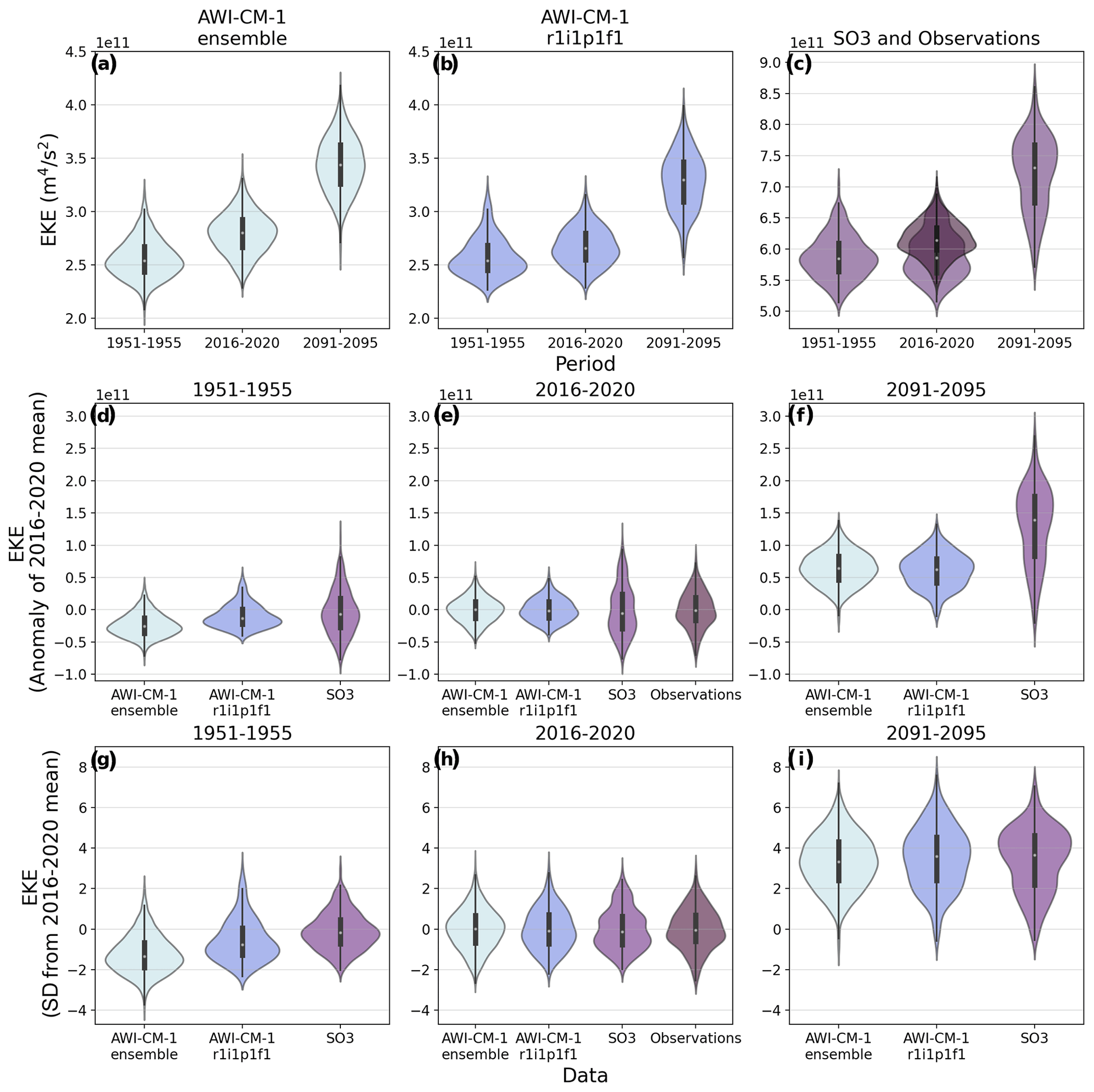
Figure 1Violin plots of area-integrated Southern Ocean EKE in simulations and observations. Central points of each plot indicate the median, thick bars span the first and third quartiles, thin bars span the range, and the violin body is a kernel density estimation of the data. (a–c) Magnitudes of area-integrated EKE (note the different y axes). (a) The AWI-CM-1 ensemble. (b) The first member of the AWI-CM-1 ensemble, from which the SO3 simulations take their atmospheric forcing. (c) The SO3 simulations and observations. (d–f) Anomalies relative to the 2016–2020 mean of area-integrated EKE for each dataset: (d) 1951–1955, (e) 2016–2020, and (f) 2091–2095. (g–i) Normalized values relative to the mean and standard deviation of EKE during the 2016–2020 period for each dataset: (g) 1951–1955, (h) 2016–2020, and (i) 2091–2095.
From a regional perspective, the SO3 simulation accurately reflects local magnitudes of observed EKE and also generally captures the spatial distribution well (Fig. 2). However, there are regional shortcomings, such as between 90 and 145∘ E. Grid resolution in this region should be sufficient to resolve eddy activity (Fig. S1), indicating that the bias arises from another source. In the AWI-CM-1 ensemble, the regional representation of EKE reinforces a broad underrepresentation relative to observed magnitudes, but the major geographic features of eddy activity are fairly well represented (Fig. 2). Once again, the ensemble spread within the AWI-CM-1 simulations reveals remarkable consistency, this time in terms of the spatial pattern and regional magnitudes (Fig. S2), reinforcing the conclusion that a single ensemble member of 5 years' duration is sufficient to assess the mean state of EKE in the Southern Ocean. The consistency of the AWI-CM-1 ensemble further suggests that regional shortcomings in eddy activity in the SO3 simulations are not a product of variability within a single realization of Southern Ocean conditions (Fig. S2).
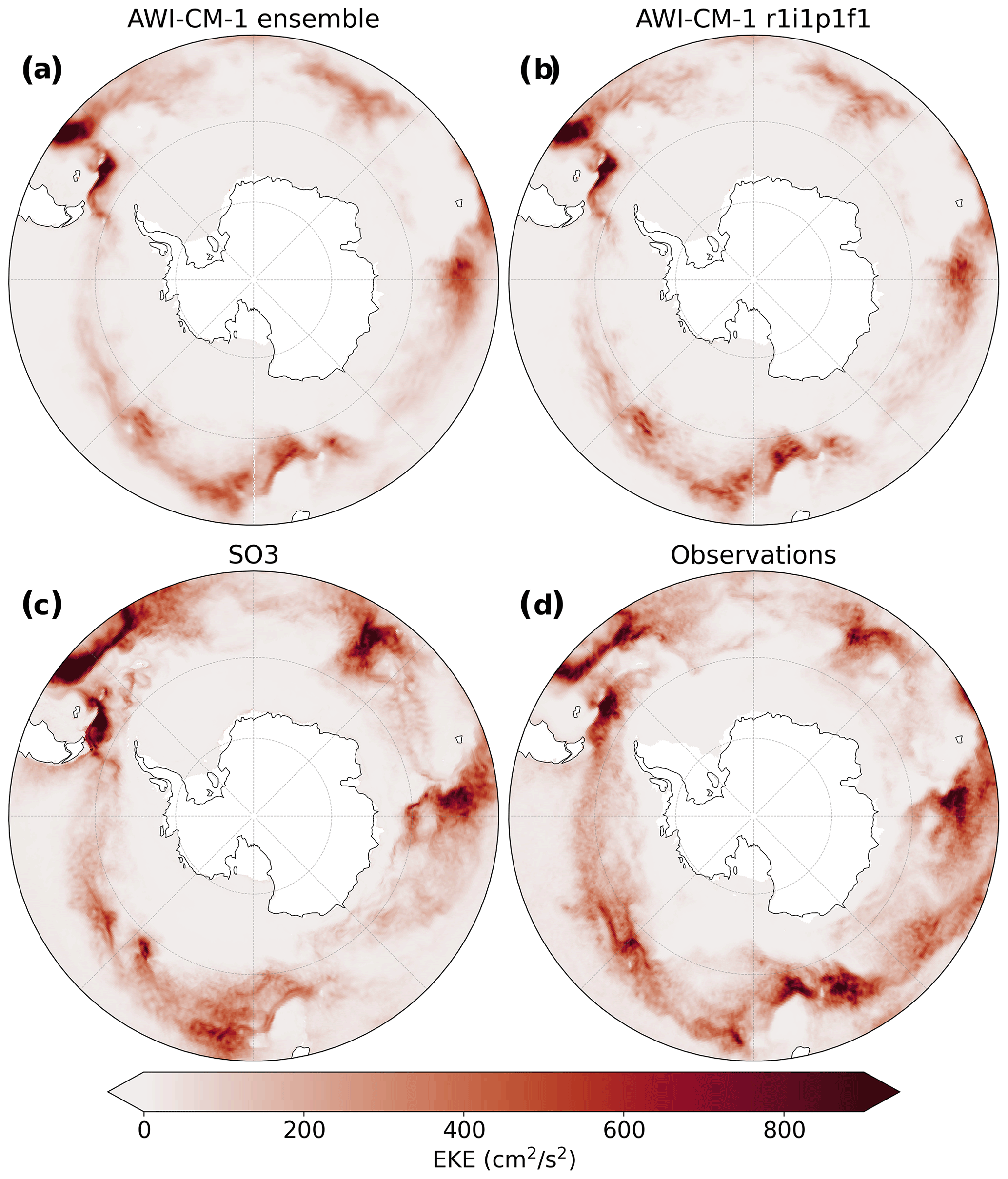
Figure 2Mean eddy kinetic energy between 2016 and 2020. (a) The AWI-CM-1 ensemble. (b) The first member of the AWI-CM-1 ensemble. (c) The SO3 simulation. (d) The gridded satellite altimetry dataset.
3.2 EKE change and significance
Southern Ocean eddy activity has been shown to have intensified over the recent decades using both satellite altimetry (Martínez-Moreno et al., 2021) and the complete AWI-CM-1-1 dataset from CMIP6 (Beech et al., 2022). Even after reducing the AWI-CM-1 CMIP6 dataset to 5-year periods preceding the apparent change (1951–1955) and at the end of the altimetry era (2016–2020), this intensification is still discernable within the AWI-CM-1 ensemble (Fig. 1a). Despite this, the SO3 simulations do not demonstrate any substantial change in EKE magnitude over the same period (Fig. 1). Further reducing the ensemble to its individual members (Fig. 3), the EKE rise is still relatively robust in each case, including clear separation of the datasets considering the median, mode, and distribution of the data. However, the first ensemble member, from which the atmospheric forcing of SO3 is taken, demonstrates less EKE rise than the ensemble average (Fig. 3), suggesting that natural variability in atmospheric conditions may contribute to the disagreement. Further investigation reveals several differences between the SO3 simulations and the AWI-CM-1 ensemble members that may play a role. Mean zonal ocean velocity in SO3 is faster and broader than the AWI-CM-1 ensemble (Fig. S3), meaning wind speed intensification may be misaligned with peak ocean velocities in SO3, particularly around 47 to 51∘ S. Moreover, considerably less zonal wind stress is imparted to the ocean in SO3 despite identical wind speeds as the first AWI-CM-1 ensemble member (Fig. S4), possibly due to the higher ocean surface velocity.
The intensification of EKE becomes clear in both the AWI-CM-1 ensemble (Fig. 1a), its members (Fig. 3), and the SO3 simulations (Fig. 1c) by the end of the 21st century. Over this period, the variability in EKE, indicated by the range of the distribution, also increases for each dataset (Fig. 1f, i). EKE rise in SO3 is approximately twice that of the AWI-CM-1 ensemble in absolute terms (Fig. 1f), but expressing EKE as a relative value normalized by the mean and standard deviation of each dataset during the observational period (Fig. 1g, h, i) reveals greater consistency between the changes until the end of the 21st century. EKE in each dataset appears to increase by approximately 3.5 standard deviations, and the range of EKE distributions increases by approximately 2 to 3 standard deviations (Fig. 1h, i). However, the datasets also tend to become more autocorrelated, which can inflate the distribution range (Tables S1, S3).
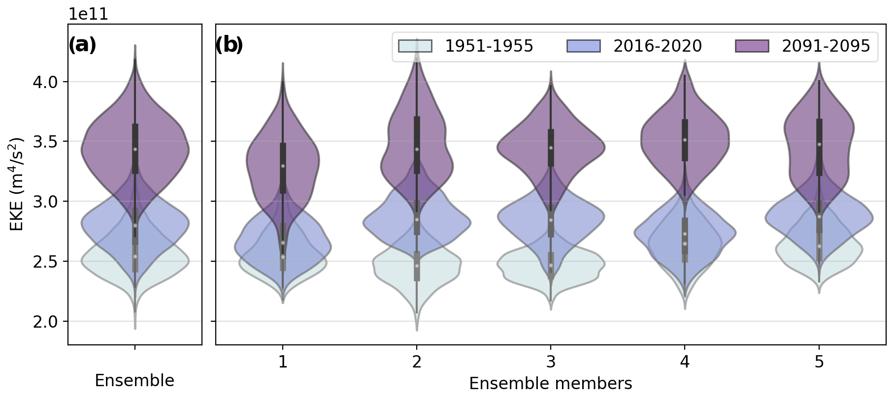
Figure 3Ensemble spread of EKE in AWI-CM-1. (a) Violin plots of area-integrated Southern Ocean EKE in the AWI-CM-1 ensemble. (b) Violin plots of mean Southern Ocean EKE in each member of the AWI-CM-1 ensemble. Grey plots represent the period 1951–1955, blue plots represent 2016–2020, and purple plots represent 2091–2095.
Before considering the regional impacts of warming on EKE in the SO3 simulations, it is useful to refer to the ensemble spread within the AWI-CM-1 simulations to approximate the reliability of a single ensemble member in revealing the ensemble-mean change as an analogue to the signal-to-noise ratio. At 1 ∘C of warming, EKE change in the ensemble is weak, with at least one ensemble member tending to show little or no EKE change in most regions (Fig. 4a, c). Only a few clear patterns of change emerge throughout the ensemble, namely the regions of EKE intensification downstream of the Kerguelen Plateau and the Campbell Plateau, where four to five out of five ensemble members show clear EKE intensification (Fig. 4a). It should be noted that even in these regions of relatively high confidence (four to five ensemble members, Fig. 4a) EKE rise can be interspersed with lower-confidence (one to two ensemble members, Fig. 4c) EKE decline; this is also illustrated by the ensemble mean changes themselves (Figs. S5, S6). Despite this, the consistency of EKE rise in these regions, as well as their geographic positions in already EKE-rich regions, suggests that the intensification patterns are robust changes within substantial noise. This level of noise suggests that EKE changes in the SO3 simulations at 1 ∘C of warming will be difficult to distinguish from natural variability when taken on their own; indeed, in the SO3 simulations, the large variability in both sign and magnitude of change within relatively small spatial scales does not lend confidence to any significant change at 1 ∘C of warming (Fig. 5c). However, building on the changes observed in the AWI-CM-1 ensemble, the intensification of EKE downstream of the Kerguelen and Campbell plateaus seems to be reinforced by the high-resolution simulations.
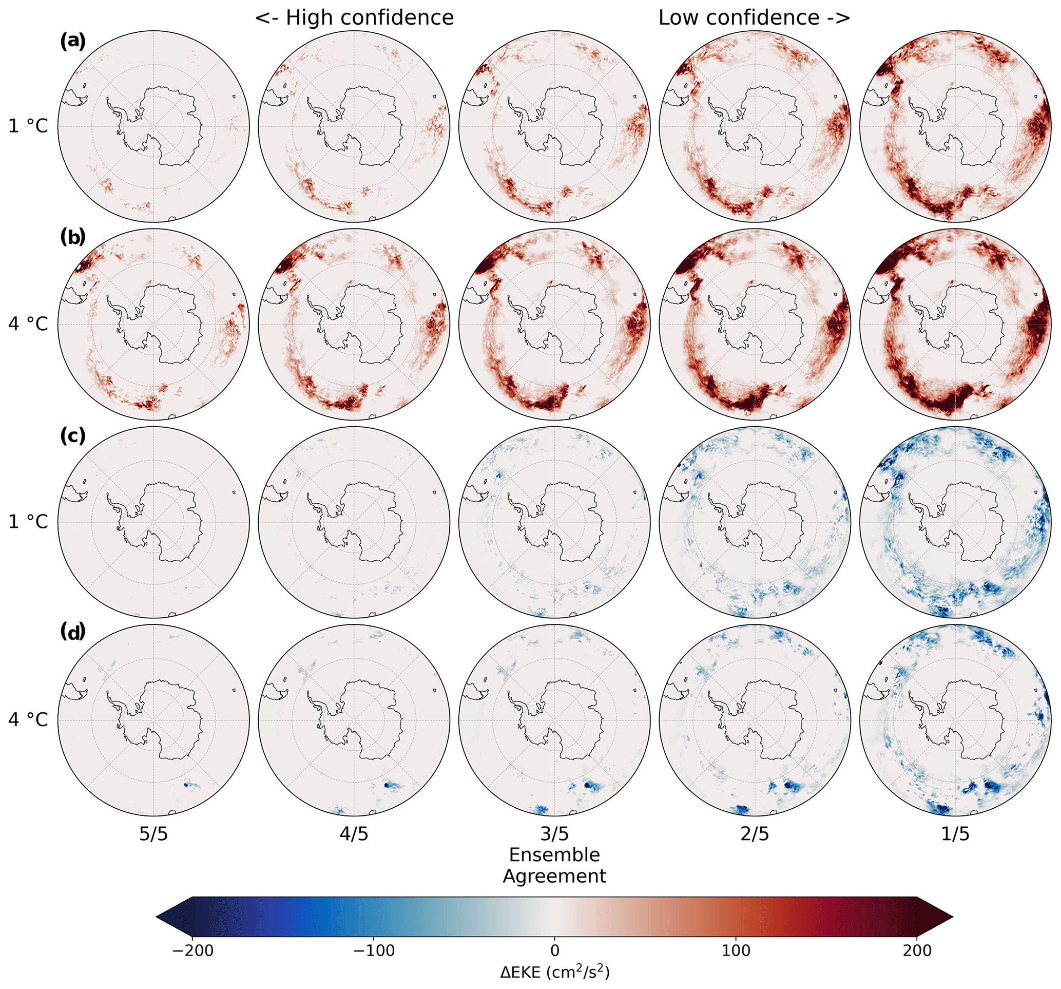
Figure 4Ensemble agreement regarding EKE change. EKE rise (a, b) and decline (c, d) within the AWI-CM-1 ensemble after 1 (a, c) and 4 ∘C (b, d) of warming or between 1951–1955 and 2016–2020 and 2091–2095, respectively, arranged in order of decreasing ensemble agreement regarding change in each grid cell. Ensemble agreement refers to the number of ensemble members that simulate at least the pictured magnitude of mean EKE rise or decline for each grid cell. Mean EKE change is defined as the difference in mean EKE between 1951–1955 and each of the two latter periods, as in Figs. S5 and S6 but arranged in ascending order of magnitude for each grid cell and for positive and negative signs separately. Rank 5/5 indicates the lowest magnitude of mean EKE rise (a, b) or decline (c, d) within the ensemble for a given grid cell, meaning the entire ensemble agrees on at least this much change. Rank 1/5 indicates the highest magnitude of EKE rise or decline within the ensemble for each grid cell, representing the upper limit of projected EKE change.
At 4 ∘C of warming, the change in eddy activity becomes clearer; EKE intensification downstream of the Kerguelen and Campbell plateaus is now consistent throughout the entire AWI-CM-1 ensemble, along with additional intensifications south of the Falkland/Malvinas Plateau, around the Conrad Rise, and along the Antarctic Slope Current at approximately 5∘ E (Fig. 4b). Four-fifths of the ensemble also include a broad increase in EKE throughout the ACC across most longitudes. Interestingly, a consistent pattern of EKE decline also emerges upstream of the Campbell Plateau in the entire ensemble (Fig. 4d). The spatial pattern of EKE rise is relatively consistent regardless of confidence, with only the magnitude increasing in the lower confidence composites (Fig. 4b). The same tendency is observable between the EKE changes at 1 and 4 ∘C of warming, where the magnitude of change is greater after further warming but follows the same spatial pattern. Thus, regions of intensification can be identified more reliably than the magnitude of change and tend to be concentrated where flow interacts with topographic features, in already eddy-rich regions (Fig. 2). Conversely, low-confidence EKE decline appears nearly throughout the Southern Ocean in at least one ensemble member but only consistently upstream of the Campbell Plateau and, to a far lesser extent, downstream of the Drake Passage and Campbell Plateau (Fig. 4d). Changes in negative sign tend to be of lower magnitude at 4 ∘C of warming than at 1 ∘C. This suggests that the general EKE response to climate change in the Southern Ocean is that of intensification, and the interspersed signals of decline tend to be the result of natural variability. Yet, small regions of high-confidence EKE decline also appear. Consequently, it would be difficult to confidently separate reliable EKE change from natural variability in simulations without an ensemble to compare with. In the SO3 simulations, EKE rise downstream of the Drake Passage and Kerguelen and Campbell plateaus is substantial (Fig. 5f). EKE rise is also projected south of the Falkland/Malvinas Plateau, around the Conrad Rise, and along the Antarctic Slope Current at approximately 5∘ E, and a slight EKE decline appears upstream of the Campbell Plateau. All of this is comparable to the AWI-CM-1 ensemble, and the interspersed areas of EKE decline within these regions, for example, around the Conrad Rise, are not improbable based on the example set by AWI-CM-1 (Fig. 4d). However, considering that some high-confidence EKE decline is present in the AWI-CM-1 ensemble, it is difficult to confidently dismiss regional EKE decline in the SO3 simulations as noise.
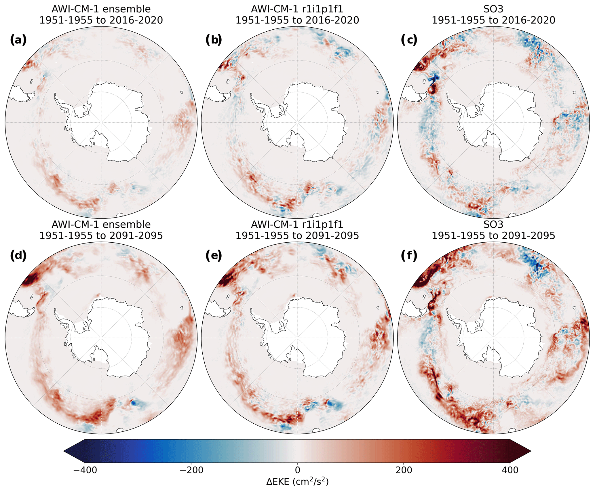
Figure 5EKE change. Spatial representations of the difference in EKE between (a–c) 1951–1955 and 2016–2020 and (d–f) 1951–1955 and 2091–2095. (a, d) The AWI-CM-1 ensemble. (b, e) The first member of the AWI-CM-1 ensemble. (c, f) The SO3 simulations.
Intensification of eddy activity in the Southern Ocean is now widely accepted as a consequence of anthropogenic climate change (Hogg et al., 2015; Patara et al., 2016; Martínez-Moreno et al., 2021; Beech et al., 2022) and is understood to be caused primarily by stronger westerly winds imparting more energy to the Antarctic Circumpolar Current (Munday et al., 2013; Marshall, 2003). The results presented here reinforce the notion of EKE intensification and further project increased EKE variability as the climate warms (Figs. 1, 3). By expressing EKE change in terms of ensemble agreement on a cell-by-cell basis, the results presented here are also able to identify regions of reliable and substantial change as those where flow interacts with major bathymetric features and high eddy activity is already known to occur (Fig. 4). Analysis of regional changes within the Southern Ocean eddy field has generally been limited to regions defined by oceanic sectors (Atlantic, Indian, Pacific) (Hogg et al., 2015) or incremental longitudinal delimitations (Patara et al., 2016). In future research, regional analyses of the significance, rate, or cause of EKE trends could focus on the bathymetrically defined regions identified in this analysis to produce physically related and consistent results.
The consistency of the AWI-CM-1 ensemble in projecting clear EKE rise in the Southern Ocean as a whole suggests that a single ensemble member of 5-year simulation length should be sufficient to reliably identify change, even after 1 ∘C of temperature rise. Despite this, the SO3 simulations fail to reproduce the EKE rise that is already observable through observations (Martínez-Moreno et al., 2021). A potential source for this discrepancy is the uncoupled model setup in the SO3 simulations which omits ocean–atmosphere feedbacks. In this regard, the SO3 simulations experience lower wind stress imparted to the ocean surface than the AWI-CM-1 ensemble member one by the same surface winds (Fig. S4), as well as a mismatch between peak zonal wind speeds and mean zonal ocean velocities (Fig. 3). Confounding the comparison further is the fact that strengthening winds can both increase and dampen eddy activity; as westerlies intensify, the additional energy imparted to the ocean is expected to strengthen eddy activity (Munday et al., 2013; Meredith and Hogg, 2006), but winds are also known to dampen mesoscale activity through eddy killing (Rai et al., 2021), and this impact is greater in uncoupled model configurations (Renault et al., 2016). While the lack of change at 1 ∘C is difficult to explain, the disagreement is limited to these more subtle changes, and the simulations tend to agree on the strong EKE rise at 4 ∘C of warming.
The remaining discrepancies between eddy activity in SO3 and observations are relatively small, but exploring potential sources of disagreement may help in interpreting the simulations and guide future modeling endeavors. Greater skew in the distribution of EKE in the modeled dataset (Table S2) could reflect multiple modes of circulation or seasonality. While seasonality of eddy activity in the ACC is low, seasonal ice cover likely affects eddy activity in the modeled dataset and certainly affects the observational dataset by producing gaps in its spatiotemporal coverage. Beyond differences in skew, this could contribute to the greater range of EKE seen in the SO3 simulations by systemically obscuring seasonal conditions from the observational dataset. Regional deficiencies of EKE in SO3 could be explained in terms of grid resolution outside of the study region; resolving the first Rossby radius of deformation with at least two grid points is not enough to comprehensively reproduce mesoscale activity (Hallberg, 2013; Sein et al., 2017), and grid refinement may need to be expanded to upstream regions that impact eddy dynamics in the Southern Ocean. Other sources of bias may include ocean–atmosphere interactions which are absent or unrealistic within the uncoupled simulations (Byrne et al., 2016; Rai et al., 2021; Renault et al., 2016). In addition, some small-scale, slow-to-equilibrate ocean processes may be resolved in the high-resolution simulations but not be integrated long enough for their effects to impact eddy activity (van Westen and Dijkstra, 2021; Rackow et al., 2022). Finally, the gridded altimetry product itself may be responsible for some disagreement, as the along-track data are known to underrepresent eddy activity at scales less than 150 km and 10 d (Chassignet and Xu, 2017), which will be particularly impactful at high latitudes.
To distinguish a meaningful signal of anthropogenic impacts from natural variability, this analysis relies primarily on consistency among ensemble members (Figs. 3, 4). This is distinct from more traditional methods like assessment of error relative to observations or ensemble mean, commonly applied to weather forecasting (Ferro et al., 2012), but they can be compared to measurements of ensemble agreement used extensively in the IPCC reports (Fox-Kemper et al., 2021). Performance evaluation relative to observations would undoubtedly point to the high-resolution simulation as being superior due to the drastic underrepresentation of EKE in the eddy-permitting ensemble (Fig. 1). Yet, the effects of climate change are still apparent in the AWI-CM-1 ensemble (Figs. 1, 5), and the AWI-CM-1 dataset has been used to make similar projections of EKE already (Beech et al., 2022). Moreover, the eddy response to forcing seems to be consistent between the model resolutions when expressed in relative (Fig. 1g, h, i) rather than absolute terms (Fig. 1a, b, c). While more verification of this result is necessary both regionally and with other models, these results suggest that eddy-permitting resolutions can be interpreted with their shortcomings in mind in order to discern the real-world implications, as is often necessary with model data. Thus, based on the test case of the Southern Ocean, the usefulness of the AWI-CM-1 ensemble and the effectiveness of model simulations in identifying physically significant and reproducible impacts of climate change may be greater than would be identified using traditional methods and comes at a much lower cost relative to the eddy-resolving simulations.
This study has focused on EKE as an evaluation metric for the simulations since mesoscale activity is the primary motivation for increasing ocean model resolution. It has stopped short of assessing the improvements that resolving the mesoscale has on climate and ocean dynamics, many of which are discussed in detail elsewhere (e.g. Hewitt et al., 2017). Rather than repeat an assessment of the benefits of resolving smaller scales, we assume that the accurate reproduction and evolution of eddy activity indicates that these improvements are transferred to broader processes. Certainly, inaccurate simulation of the mesoscale would raise questions regarding the improvements that this mesoscale activity should have on the simulations as a whole. Nonetheless, further evaluation of the modeling approaches employed in this study will be necessary to determine if these methods are appropriate for studying broader elements of the climate system. Since the high-resolution simulations derive their deep-ocean climate primarily from the medium-resolution spin-up simulation, improving the initialization process (Thiria et al., 2023) may be the critical barrier to extending these results from the mixed layer to the deeper ocean.
Resolving the ocean mesoscale has become a focus for the climate and ocean modeling community as computational capabilities expand and models become increasingly complex. The benefits that explicitly resolved eddy activity can have on climate simulations are clear (Hewitt et al., 2017; Sein et al., 2017) along with the impact that mesoscale variability has on local (Lachkar et al., 2009; Wang et al., 2017) and global environments (Falkowski et al., 1991; Sallée et al., 2012). However, state-of-the-art climate models will be unable to fully resolve the mesoscale for the foreseeable future, particularly in large-scale modeling endeavors such as CMIP (Hewitt et al., 2020). Thus, modelers must make informed choices regarding the explicit processes needed to answer research questions and where resources must be allocated to achieve specific goals. Existing analysis of resource allocation has typically addressed short-term weather forecasting or the ability to reproduce observations with low error (Ferro et al., 2012), but the question of how to best allocate resources for climate change impact assessment remains. This study has applied several cost-efficient modeling approaches to an analysis of the impacts of climate change on a key focus of high-resolution modeling: the mesoscale. Applying these results to broader climate change impact studies should improve the efficiency of resource allocation and focus modeling studies. Resolution can be dynamically adjusted both spatially, by focusing resources in study regions and where they are necessary to resolve local dynamics, and temporally, by allowing lower-resolution workhorse configurations to perform spin-up and transient runs. Limited simulation length and ensemble size can be sufficient for certain research questions and validation, but simulations must ultimately be designed to meet their specific goals. Where resources are limited, studies may best include a combination of eddy-resolving simulations able to fully capture the local eddy field, as well as eddy-permitting simulations that can attest to the significance of results through consistency and repetition.
This work represents a contribution to the growing wealth of research that points to an intensification of eddy activity in the Southern Ocean (Hogg et al., 2015; Martínez-Moreno et al., 2021; Beech et al., 2022). The further conclusions that EKE variability may increase and that EKE intensification appears concentrated in key regions based on topography can both expand the present state of knowledge and direct future research. The cost-efficient modeling approaches of regional grid refinement, reduced-resolution spin-up and transient runs, and limited simulation lengths distinguished by longer periods of change are demonstrated to be effective at reproducing change within a more traditional eddy-permitting ensemble. When resources are limited and resolution demands are high, these approaches can be adapted to address specific research questions. Where assessing the robustness of change is critical, the complementary eddy-permitting ensemble represents an effective, low-cost supplement to the high-resolution simulations.
Geostrophic velocities derived from satellite altimetry data are publicly available at https://doi.org/10.48670/moi-00148 (CMEMS, 2022). Daily sea surface height data from AWI-CM-1-1-MR in CMIP6 used to compute geostrophic velocities in this study are archived at the World Data Center for Climate at the DKRZ (https://doi.org/10.26050/WDCC/C6sCMAWAWM, https://doi.org/10.26050/WDCC/C6sSPAWAWM) (Semmler et al., 2022a, b). Model output from AWI-CM-1-1-MR in the CMIP6 framework, including all variables used to force the standalone ocean simulations conducted for this study, is publicly available at https://doi.org/10.22033/ESGF/CMIP6.359 (Semmler et al., 2018). Eddy kinetic energy datasets calculated from FESOM output velocities are available at https://doi.org/10.5281/zenodo.8046792 (Beech, 2023b). Source code for the ocean model FESOM2 is available at https://doi.org/10.5281/zenodo.10476072 (Danilov et al., 2024). Code used for data analysis and visualization in this study is publicly available at https://doi.org/10.5281/zenodo.8046782 (Beech, 2023a). The code used to calculate geostrophic velocities from sea surface height data from AWI-CM-1-1-MR is available from https://doi.org/10.5281/zenodo.7050573 (Beech, 2022).
The supplement related to this article is available online at: https://doi.org/10.5194/gmd-17-529-2024-supplement.
NB, TJ, TR, and TS conceived of the study. NB carried out the simulations, analyzed the data, and drafted the manuscript. All authors reviewed the manuscript.
The contact author has declared that none of the authors has any competing interests.
Publisher’s note: Copernicus Publications remains neutral with regard to jurisdictional claims made in the text, published maps, institutional affiliations, or any other geographical representation in this paper. While Copernicus Publications makes every effort to include appropriate place names, the final responsibility lies with the authors.
The work described in this paper has received funding from the Helmholtz Association through the project “Advanced Earth System Model Capacity” (project leader: Thomas Jung; support code: ZT-0003) in the frame of the initiative “Zukunftsthemen”. The content of the paper is the sole responsibility of the authors, and it does not represent the opinion of the Helmholtz Association, and the Helmholtz Association is not responsible for any use that might be made of information contained. Thomas Jung acknowledges the EERIE project funded under the European Commission, Horizon 2020 framework programme (grant number 101081383). The CMIP6 data used in this study were replicated and made available by the DKRZ.
This research has been supported by the Helmholtz Association (grant no. ZT-0003); the European Commission, Horizon 2020 Framework Programme (grant no. 101003470); and the Deutsches Klimarechenzentrum (grant no. 995).
The article processing charges for this open-access publication were covered by the Alfred-Wegener-Institut Helmholtz-Zentrum für Polar- und Meeresforschung.
This paper was edited by Riccardo Farneti and reviewed by Mark R. Petersen and one anonymous referee.
Auger, M., Prandi, P., and Sallée, J.-B.: Southern ocean sea level anomaly in the sea ice-covered sector from multimission satellite observations, Sci. Data, 9, 70, https://doi.org/10.1038/s41597-022-01166-z, 2022.
Auger, M., Sallée, J.-B., Thompson, A. F., Pauthenet, E., and Prandi, P.: Southern Ocean Ice-Covered Eddy Properties From Satellite Altimetry, J. Geophys. Res.-Oceans, 128, e2022JC019363, https://doi.org/10.1029/2022JC019363, 2023.
Ballarotta, M., Ubelmann, C., Pujol, M.-I., Taburet, G., Fournier, F., Legeais, J.-F., Faugère, Y., Delepoulle, A., Chelton, D., Dibarboure, G., and Picot, N.: On the resolutions of ocean altimetry maps, Ocean Sci., 15, 1091–1109, https://doi.org/10.5194/os-15-1091-2019, 2019.
Beech, N.: n-beech/awicm-cmip6-eke: Inititial (v1.1), Zenodo [code], https://doi.org/10.5281/zenodo.7050573, 2022.
Beech, N.: n-beech/Beech_et_al_cost_efficient_SO: Final, Zenodo [code], https://doi.org/10.5281/zenodo.10185411, 2023a.
Beech, N.: Processed EKE from FESOM-SO3 (1.0), Zenodo [data set], https://doi.org/10.5281/zenodo.8046792, 2023b.
Beech, N., Rackow, T., Semmler, T., Danilov, S., Wang, Q., and Jung, T.: Long-term evolution of ocean eddy activity in a warming world, Nat. Clim. Change, 12, 910–917, https://doi.org/10.1038/s41558-022-01478-3, 2022.
Bishop, S. P., Gent, P. R., Bryan, F. O., Thompson, A. F., Long, M. C., and Abernathey, R.: Southern Ocean Overturning Compensation in an Eddy-Resolving Climate Simulation, J. Phys. Oceanogr., 46, 1575–1592, https://doi.org/10.1175/JPO-D-15-0177.1, 2016.
Bronselaer, B., Winton, M., Griffies, S. M., Hurlin, W. J., Rodgers, K. B., Sergienko, O. V., Stouffer, R. J., and Russell, J. L.: Change in future climate due to Antarctic meltwater, Nature, 564, 53–58, https://doi.org/10.1038/s41586-018-0712-z, 2018.
Byrne, D., Münnich, M., Frenger, I., and Gruber, N.: Mesoscale atmosphere ocean coupling enhances the transfer of wind energy into the ocean, Nat. Commun., 7, ncomms11867, https://doi.org/10.1038/ncomms11867, 2016.
Chassignet, E. P. and Xu, X.: Impact of Horizontal Resolution (1/12∘ to 1/50∘) on Gulf Stream Separation, Penetration, and Variability, J. Phys. Oceanogr., 47, 1999–2021, https://doi.org/10.1175/JPO-D-17-0031.1, 2017.
D'Agostino, R. B. and Belanger, A.: A Suggestion for Using Powerful and Informative Tests of Normality, Am. Stat., 44, 316–321, https://doi.org/10.2307/2684359, 1990.
Danilov, S.: Ocean modeling on unstructured meshes, Ocean Model., 69, 195–210, https://doi.org/10.1016/j.ocemod.2013.05.005, 2013.
Danilov, S.: On the Resolution of Triangular Meshes, J. Adv. Model. Earth Sy., 14, e2022MS003177, https://doi.org/10.1029/2022MS003177, 2022.
Danilov, S., Sidorenko, D., Wang, Q., and Jung, T.: The Finite-volumE Sea ice–Ocean Model (FESOM2), Geosci. Model Dev., 10, 765–789, https://doi.org/10.5194/gmd-10-765-2017, 2017.
Danilov, S., Sidorenko, D., Koldunov, N., Scholz, P., Wang, Q., Rackow, T., Helge, G., and Zampieri, L.: FESOM2.5_SO3, Zenodo [code], https://doi.org/10.5281/zenodo.10476072, 2024.
Durbin, J. and Watson, G. S.: Testing for Serial Correlation in Least Squares Regression. I, Biometrika, 37, 409–428, https://doi.org/10.1093/biomet/37.3-4.409, 1950.
E.U. Copernicus Marine Service Information (CMEMS): Global Ocean Gridded L 4 Sea Surface Heights And Derived Variables Reprocessed 1993 Ongoing, Marine Data Store (MDS) [data set], https://doi.org/10.48670/moi-00148, 2022.
Eyring, V., Bony, S., Meehl, G. A., Senior, C. A., Stevens, B., Stouffer, R. J., and Taylor, K. E.: Overview of the Coupled Model Intercomparison Project Phase 6 (CMIP6) experimental design and organization, Geosci. Model Dev., 9, 1937–1958, https://doi.org/10.5194/gmd-9-1937-2016, 2016.
Falkowski, P. G., Ziemann, D., Kolber, Z., and Bienfang, P. K.: Role of eddy pumping in enhancing primary production in the ocean, Nature, 352, 55–58, https://doi.org/10.1038/352055a0, 1991.
Ferrari, R., Griffies, S. M., Nurser, A. J. G., and Vallis, G. K.: A boundary-value problem for the parameterized mesoscale eddy transport, Ocean Model., 32, 143–156, https://doi.org/10.1016/j.ocemod.2010.01.004, 2010.
Ferro, C. A. T., Jupp, T. E., Lambert, F. H., Huntingford, C., and Cox, P. M.: Model complexity versus ensemble size: allocating resources for climate prediction, Philos. T. Roy. Soc. A, 370, 1087–1099, https://doi.org/10.1098/rsta.2011.0307, 2012.
Fisher, R. A.: The moments of the distribution for normal samples of measures of departure from normality, P. R. Soc. Lond. A-Conta., 130, 16–28, https://doi.org/10.1098/rspa.1930.0185, 1997.
Frölicher, T. L., Sarmiento, J. L., Paynter, D. J., Dunne, J. P., Krasting, J. P., and Winton, M.: Dominance of the Southern Ocean in Anthropogenic Carbon and Heat Uptake in CMIP5 Models, J. Climate, 28, 862–886, https://doi.org/10.1175/JCLI-D-14-00117.1, 2015.
Gent, P. R. and McWilliams, J. C.: Isopycnal Mixing in Ocean Circulation Models, J. Phys. Oceanogr., 20, 150–155, https://doi.org/10.1175/1520-0485(1990)020<0150:IMIOCM>2.0.CO;2, 1990.
Haarsma, R. J., Roberts, M. J., Vidale, P. L., Senior, C. A., Bellucci, A., Bao, Q., Chang, P., Corti, S., Fučkar, N. S., Guemas, V., von Hardenberg, J., Hazeleger, W., Kodama, C., Koenigk, T., Leung, L. R., Lu, J., Luo, J.-J., Mao, J., Mizielinski, M. S., Mizuta, R., Nobre, P., Satoh, M., Scoccimarro, E., Semmler, T., Small, J., and von Storch, J.-S.: High Resolution Model Intercomparison Project (HighResMIP v1.0) for CMIP6, Geosci. Model Dev., 9, 4185–4208, https://doi.org/10.5194/gmd-9-4185-2016, 2016.
Hallberg, R.: Using a resolution function to regulate parameterizations of oceanic mesoscale eddy effects, Ocean Model., 72, 92–103, https://doi.org/10.1016/j.ocemod.2013.08.007, 2013.
Hewitt, H. T., Bell, M. J., Chassignet, E. P., Czaja, A., Ferreira, D., Griffies, S. M., Hyder, P., McClean, J. L., New, A. L., and Roberts, M. J.: Will high-resolution global ocean models benefit coupled predictions on short-range to climate timescales?, Ocean Model., 120, 120–136, https://doi.org/10.1016/j.ocemod.2017.11.002, 2017.
Hewitt, H. T., Roberts, M., Mathiot, P., Biastoch, A., Blockley, E., Chassignet, E. P., Fox-Kemper, B., Hyder, P., Marshall, D. P., Popova, E., Treguier, A.-M., Zanna, L., Yool, A., Yu, Y., Beadling, R., Bell, M., Kuhlbrodt, T., Arsouze, T., Bellucci, A., Castruccio, F., Gan, B., Putrasahan, D., Roberts, C. D., Van Roekel, L., and Zhang, Q.: Resolving and Parameterising the Ocean Mesoscale in Earth System Models, Curr. Clim. Change Rep., 6, 137–152, https://doi.org/10.1007/s40641-020-00164-w, 2020.
Hogg, A. McC., Meredith, M. P., Chambers, D. P., Abrahamsen, E. P., Hughes, C. W., and Morrison, A. K.: Recent trends in the Southern Ocean eddy field, J. Geophys. Res.-Oceans, 120, 257–267, https://doi.org/10.1002/2014JC010470, 2015.
Irving, D., Hobbs, W., Church, J., and Zika, J.: A Mass and Energy Conservation Analysis of Drift in the CMIP6 Ensemble, J. Climate, 34, 3157–3170, https://doi.org/10.1175/JCLI-D-20-0281.1, 2021.
Jungclaus, J. H., Lorenz, S. J., Schmidt, H., Brovkin, V., Brüggemann, N., Chegini, F., Crüger, T., De-Vrese, P., Gayler, V., Giorgetta, M. A., Gutjahr, O., Haak, H., Hagemann, S., Hanke, M., Ilyina, T., Korn, P., Kröger, J., Linardakis, L., Mehlmann, C., Mikolajewicz, U., Müller, W. A., Nabel, J. E. M. S., Notz, D., Pohlmann, H., Putrasahan, D. A., Raddatz, T., Ramme, L., Redler, R., Reick, C. H., Riddick, T., Sam, T., Schneck, R., Schnur, R., Schupfner, M., von Storch, J.-S., Wachsmann, F., Wieners, K.-H., Ziemen, F., Stevens, B., Marotzke, J., and Claussen, M.: The ICON Earth System Model Version 1.0, J. Adv. Model. Earth Sy., 14, e2021MS002813, https://doi.org/10.1029/2021MS002813, 2022.
Lachkar, Z., Orr, J. C., Dutay, J. C., and Delecluse, P.: On the role of mesoscale eddies in the ventilation of Antarctic intermediate water, Deep-Sea Res. Pt. I, 56, 909–925, https://doi.org/10.1016/j.dsr.2009.01.013, 2009.
Landschützer, P., Gruber, N., Haumann, F. A., Rödenbeck, C., Bakker, D. C. E., van Heuven, S., Hoppema, M., Metzl, N., Sweeney, C., Takahashi, T., Tilbrook, B., and Wanninkhof, R.: The reinvigoration of the Southern Ocean carbon sink, Science, 349, 1221–1224, https://doi.org/10.1126/science.aab2620, 2015.
Large, W. G., McWilliams, J. C., and Doney, S. C.: Oceanic vertical mixing: A review and a model with a nonlocal boundary layer parameterization, Rev. Geophys., 32, 363–403, https://doi.org/10.1029/94RG01872, 1994.
Marshall, G. J.: Trends in the Southern Annular Mode from Observations and Reanalyses, J. Climate, 16, 4134–4143, https://doi.org/10.1175/1520-0442(2003)016<4134:TITSAM>2.0.CO;2, 2003.
Marshall, J., Jones, H., Karsten, R., and Wardle, R.: Can Eddies Set Ocean Stratification?, J. Phys. Oceanogr., 32, 26–38, https://doi.org/10.1175/1520-0485(2002)032<0026:CESOS>2.0.CO;2, 2002.
Martínez-Moreno, J., Hogg, A. McC., England, M. H., Constantinou, N. C., Kiss, A. E., and Morrison, A. K.: Global changes in oceanic mesoscale currents over the satellite altimetry record, Nat. Clim. Change, 11, 397–403, https://doi.org/10.1038/s41558-021-01006-9, 2021.
Marzocchi, A., Hirschi, J. J.-M., Holliday, N. P., Cunningham, S. A., Blaker, A. T., and Coward, A. C.: The North Atlantic subpolar circulation in an eddy-resolving global ocean model, J. Marine Syst., 142, 126–143, https://doi.org/10.1016/j.jmarsys.2014.10.007, 2015.
Meredith, M. P. and Hogg, A. M.: Circumpolar response of Southern Ocean eddy activity to a change in the Southern Annular Mode, Geophys. Res. Lett., 33, L16608, https://doi.org/10.1029/2006GL026499, 2006.
Munday, D. R., Johnson, H. L., and Marshall, D. P.: Eddy Saturation of Equilibrated Circumpolar Currents, J. Phys. Oceanogr., 43, 507–532, https://doi.org/10.1175/JPO-D-12-095.1, 2013.
O'Neill, B. C., Tebaldi, C., van Vuuren, D. P., Eyring, V., Friedlingstein, P., Hurtt, G., Knutti, R., Kriegler, E., Lamarque, J.-F., Lowe, J., Meehl, G. A., Moss, R., Riahi, K., and Sanderson, B. M.: The Scenario Model Intercomparison Project (ScenarioMIP) for CMIP6, Geosci. Model Dev., 9, 3461–3482, https://doi.org/10.5194/gmd-9-3461-2016, 2016.
O'Neill, B. C., Kriegler, E., Ebi, K. L., Kemp-Benedict, E., Riahi, K., Rothman, D. S., van Ruijven, B. J., van Vuuren, D. P., Birkmann, J., Kok, K., Levy, M., and Solecki, W.: The roads ahead: Narratives for shared socioeconomic pathways describing world futures in the 21st century, Glob. Environ. Change, 42, 169–180, https://doi.org/10.1016/j.gloenvcha.2015.01.004, 2017.
Patara, L., Böning, C. W., and Biastoch, A.: Variability and trends in Southern Ocean eddy activity in 1/12∘ ocean model simulations, Geophys. Res. Lett., 43, 4517–4523, https://doi.org/10.1002/2016GL069026, 2016.
Pauling, A. G., Smith, I. J., Langhorne, P. J., and Bitz, C. M.: Time-Dependent Freshwater Input From Ice Shelves: Impacts on Antarctic Sea Ice and the Southern Ocean in an Earth System Model, Geophys. Res. Lett., 44, 10454–10461, https://doi.org/10.1002/2017GL075017, 2017.
Price, J. F., Weller, R. A., and Schudlich, R. R.: Wind-Driven Ocean Currents and Ekman Transport, Science, 238, 1534–1538, https://doi.org/10.1126/science.238.4833.1534, 1987.
Rackow, T., Danilov, S., Goessling, H. F., Hellmer, H. H., Sein, D. V., Semmler, T., Sidorenko, D., and Jung, T.: Delayed Antarctic sea-ice decline in high-resolution climate change simulations, Nat. Commun., 13, 637, https://doi.org/10.1038/s41467-022-28259-y, 2022.
Rai, S., Hecht, M., Maltrud, M., and Aluie, H.: Scale of oceanic eddy killing by wind from global satellite observations, Sci. Adv., 7, eabf4920, https://doi.org/10.1126/sciadv.abf4920, 2021.
Renault, L., Molemaker, M. J., McWilliams, J. C., Shchepetkin, A. F., Lemarié, F., Chelton, D., Illig, S., and Hall, A.: Modulation of Wind Work by Oceanic Current Interaction with the Atmosphere, J. Phys. Oceanogr., 46, 1685–1704, https://doi.org/10.1175/JPO-D-15-0232.1, 2016.
Ringler, T., Petersen, M., Higdon, R. L., Jacobsen, D., Jones, P. W., and Maltrud, M.: A multi-resolution approach to global ocean modeling, Ocean Model., 69, 211–232, https://doi.org/10.1016/j.ocemod.2013.04.010, 2013.
Sallée, J.-B., Matear, R. J., Rintoul, S. R., and Lenton, A.: Localized subduction of anthropogenic carbon dioxide in the Southern Hemisphere oceans, Nat. Geosci., 5, 579–584, https://doi.org/10.1038/ngeo1523, 2012.
Scholz, P., Sidorenko, D., Gurses, O., Danilov, S., Koldunov, N., Wang, Q., Sein, D., Smolentseva, M., Rakowsky, N., and Jung, T.: Assessment of the Finite-volumE Sea ice-Ocean Model (FESOM2.0) – Part 1: Description of selected key model elements and comparison to its predecessor version, Geosci. Model Dev., 12, 4875–4899, https://doi.org/10.5194/gmd-12-4875-2019, 2019.
Scholz, P., Sidorenko, D., Danilov, S., Wang, Q., Koldunov, N., Sein, D., and Jung, T.: Assessment of the Finite-VolumE Sea ice–Ocean Model (FESOM2.0) – Part 2: Partial bottom cells, embedded sea ice and vertical mixing library CVMix, Geosci. Model Dev., 15, 335–363, https://doi.org/10.5194/gmd-15-335-2022, 2022.
Sein, D. V., Koldunov, N. V., Danilov, S., Wang, Q., Sidorenko, D., Fast, I., Rackow, T., Cabos, W., and Jung, T.: Ocean Modeling on a Mesh With Resolution Following the Local Rossby Radius, J. Adv. Model. Earth Sy., 9, 2601–2614, https://doi.org/10.1002/2017MS001099, 2017.
Semmler, T., Danilov, S., Rackow, T., Sidorenko, D., Barbi, D., Hegewald, J., Sein, D., Wang, Q., and Jung, T.: AWI AWI-CM1.1MR model output prepared for CMIP6 CMIP, Earth System Grid Federation [data set], https://doi.org/10.22033/ESGF/CMIP6.359, 2018.
Semmler, T., Danilov, S., Gierz, P., Goessling, H. F., Hegewald, J., Hinrichs, C., Koldunov, N., Khosravi, N., Mu, L., Rackow, T., Sein, D. V., Sidorenko, D., Wang, Q., and Jung, T.: Simulations for CMIP6 With the AWI Climate Model AWI-CM-1-1, J. Adv. Model. Earth Sy., 12, e2019MS002009, https://doi.org/10.1029/2019MS002009, 2020.
Semmler, T., Danilov, S., Rackow, T., Sidorenko, D., Barbi, D., Hegewald, J., Sein, D., Wang, Q., and Jung, T.: CMIP6_supplemental CMIP AWI AWI-CM-1-1-MR, World Data Center for Climate (WDCC) at DKRZ [data set], https://doi.org/10.26050/WDCC/C6sCMAWAWM, 2022a.
Semmler, T., Danilov, S., Rackow, T., Sidorenko, D., Barbi, D., Hegewald, J., Sein, D., Wang, Q., and Jung, T.: CMIP6_supplemental ScenarioMIP AWI AWI-CM-1-1-MR, World Data Center for Climate (WDCC) at DKRZ [data set], https://doi.org/10.26050/WDCC/C6sSPAWAWM, 2022b.
Taburet, G., Sanchez-Roman, A., Ballarotta, M., Pujol, M.-I., Legeais, J.-F., Fournier, F., Faugere, Y., and Dibarboure, G.: DUACS DT2018: 25 years of reprocessed sea level altimetry products, Ocean Sci., 15, 1207–1224, https://doi.org/10.5194/os-15-1207-2019, 2019.
Thiria, S., Sorror, C., Archambault, T., Charantonis, A., Bereziat, D., Mejia, C., Molines, J.-M., and Crépon, M.: Downscaling of ocean fields by fusion of heterogeneous observations using Deep Learning algorithms, Ocean Model., 182, 102174, https://doi.org/10.1016/j.ocemod.2023.102174, 2023.
Wang, Q., Danilov, S., Sidorenko, D., Timmermann, R., Wekerle, C., Wang, X., Jung, T., and Schröter, J.: The Finite Element Sea Ice-Ocean Model (FESOM) v.1.4: formulation of an ocean general circulation model, Geosci. Model Dev., 7, 663–693, https://doi.org/10.5194/gmd-7-663-2014, 2014.
Wang, Y., Claus, M., Greatbatch, R. J., and Sheng, J.: Decomposition of the Mean Barotropic Transport in a High-Resolution Model of the North Atlantic Ocean, Geophys. Res. Lett., 44, 11537–11546, https://doi.org/10.1002/2017GL074825, 2017.
van Westen, R. M. and Dijkstra, H. A.: Ocean eddies strongly affect global mean sea-level projections, Sci. Adv., 7, eabf1674, https://doi.org/10.1126/sciadv.abf1674, 2021.
Yu, X., Ponte, A. L., Lahaye, N., Caspar-Cohen, Z., and Menemenlis, D.: Geostrophy Assessment and Momentum Balance of the Global Oceans in a Tide- and Eddy-Resolving Model, J. Geophys. Res.-Oceans, 126, e2021JC017422, https://doi.org/10.1029/2021JC017422, 2021.