Simulation of marine stratocumulus using the super-droplet method: numerical convergence and comparison to a double-moment bulk scheme using SCALE-SDM 5.2.6-2.3.1

The super-droplet method (SDM) is a Lagrangian particle-based numerical scheme for cloud microphysics. In this work, a series of simulations based on the DYCOMS-II (RF02) setup with different horizontal and vertical resolutions are conducted to explore the grid convergence of the SDM simulations of marine stratocumulus. The results are compared with the double-moment bulk scheme (SN14) and model intercomparison project (MIP) results. In general, all SDM and SN14 variables show a good agreement with the MIP results and have similar grid size dependencies. The stratocumulus simulation is more sensitive to the vertical resolution than to the horizontal resolution. The vertical grid length DZ ≪ 2.5 m is necessary for both SDM and SN14. The horizontal grid length DX < 12.5 m is necessary for the SDM simulations. DX ≤ 25 m is sufficient for SN14. We also assess the numerical convergence with respect to the super-droplet numbers. The simulations are well converged when the super-droplet number concentration (SDNC) is larger than 16 super-droplets per cell. Our results indicate that the super-droplet number per grid cell is more critical than that per unit volume at least for the stratocumulus case investigated here. Our comprehensive analysis not only offers guidance on numerical settings essential for accurate stratocumulus cloud simulation but also underscores significant differences in liquid water content and cloud macrostructure between SDM and SN14. These differences are attributed to the inherent modeling strategies of the two schemes. SDM's dynamic representation of aerosol size distribution through wet deposition markedly contrasts with SN14's static approach, influencing cloud structure and behavior over a 6 h simulation. Findings reveal sedimentation's crucial role in altering aerosol distributions near cloud tops, affecting the vertical profile of cloud fraction (CF). Additionally, the study briefly addresses numerical diffusion's potential effects, suggesting further investigation is needed. The results underscore the importance of accurate aerosol modeling and its interactions with cloud processes in marine stratocumulus simulations, pointing to future research directions for enhancing stratocumulus modeling accuracy and predictive capabilities.

1 Introduction

Marine stratocumulus clouds cover approximately one-quarter of the Earth's surface and play an important role in the planet's radiation budget (Wood, 2012; Matheou and Teixeira, 2019; Nowak et al., 2021). These clouds reflect the incident shortwave radiation and almost have no effect on the outgoing longwave radiation, resulting in a negative radiation flux (Wood, 2012). The temperature projection uncertainty in global warming simulation is mainly caused by the representation of marine low clouds in global climate models (Stephens, 2005; Bony and Dufresne, 2005; Bony et al., 2006; Boucher et al., 2013; Zelinka et al., 2020; Kawai and Shige, 2020); thus, the stratocumulus must be accurately represented in numerical models. The IPCC (AR6) states that aerosol–cloud-related processes introduce the greatest uncertainty among the radiative forcing assessment methods of major factors in the earth–atmosphere system. Therefore, we must understand the aerosol–cloud interaction of the stratocumulus.

In the cloud modeling community, two types of methods are commonly used to represent clouds in numerical models. The first type is to treat the cloud as a continuum in the Eulerian framework, namely Eulerian cloud models (ECMs). The second type is to treat the cloud as an ensemble of individual particles in the Lagrangian framework, that is, the Lagrangian particle-based cloud models (LCMs).

The bulk scheme (Kessler, 1969; Lin et al., 1983; Schoenberg Ferrier, 1994; Milbrandt and Yau, 2005) is one of the most widely used Eulerian microphysical schemes. It assumes a specific distribution (e.g., gamma distribution) to characterize the size distributions of aerosol and cloud particles; thus, only several predictors must be considered. This method is numerically efficient and saves computing resources. However, the cloud droplet size distribution (DSD) of the bulk scheme is a fixed and continuous function; thus, the calculation of microphysical processes depends on the set function properties, and the uncertainty of the cloud simulation results is high (Khain et al., 2015).

Another ECM category represents the cloud hydrometeors in discrete bins and is called the spectral bin microphysics scheme (Khain et al., 2000; Lynn et al., 2005; Morrison and Grabowski, 2010; Xue et al., 2010, 2012; Geresdi et al., 2017), which can explicitly predict the particle size or mass distribution but is computationally more costly. As a result, bin schemes suffer from the limitation of dimensionality (Shima, 2008; Shima et al., 2009; Grabowski et al., 2019). Most bin schemes are one-dimensional, which means they only predict the droplet size or mass distributions. The solute composition, mass, and soluble fraction within the cloud droplet all affect the droplet growth rate and determine the characteristics of particles remaining after the droplet has completely evaporated. In some cases, these factors are essential but are difficult to consider in the bin schemes (Shima, 2008; Shima et al., 2009; Grabowski et al., 2019; Dziekan et al., 2021). Another problem in bin microphysics comes from the limitation of the Smoluchowski equation used to represent the collision–condensation process (Smoluchowski, 1916). The Smoluchowski equation is deterministic, while the collision–coalescence of droplets is a stochastic process. Therefore, droplet collision, other than expected, can appear. The Smoluchowski equation also does not accurately predict even the mean behavior when the well-mixed volume is small, and the droplet discreteness is evident (see Alfonso and Raga, 2017; Dziekan and Pawlowska, 2017; Grabowski et al., 2019, and references therein). In addition, all ECMs are affected by numerical diffusion, which can lead to a simulated system that behaves differently from the expected physical system (Schoeffler, 1982). In bin microphysics, numerical diffusion results in the broadening of the unphysical droplet size distribution (Morrison et al., 2018; Grabowski et al., 2019). Due to the three abovementioned issues, ECMs still face difficulties in accurately simulating cloud microphysical processes. However, the recently developed Lagrangian particle-based method may be a viable solution for representing cloud and precipitation particle populations (Morrison et al., 2020).

Shima et al. (2009) proposed an LCM, called the super-droplet method (SDM), in which each super-droplet represents multiple numbers of aerosol/cloud/precipitation particles with the same attributes and position. The SDM has no numerical diffusion of liquid water and can provide more detailed microphysics information. Note that sub-grid-scale (SGS) diffusions are not represented in the original SDM, which may lead to under-diffused supersaturation and accelerate the mixing process (Grabowski and Abade, 2017; Abade et al., 2018; Hoffmann et al., 2019). The Monte Carlo collision–coalescence algorithm of the SDM is based on the stochastic process of collision–coalescence; hence, the SDM can be applied, even when the Smoluchowski equation is invalid (Dziekan and Pawlowska, 2017). Shima et al. (2009) theoretically estimated that when the number of attributes, which range from 2 to 4, becomes larger than a certain critical value, the SDM becomes computationally more efficient than the bin microphysics approach. With the increase in the supercomputer computing capacity, the number of studies using the SDM or other LCMs has increased in the past 10 years (e.g., Arabas and Shima, 2013; Naumann and Seifert, 2015; Dziekan and Pawlowska, 2017; Sato et al., 2017, 2018; Grabowski et al., 2018; Jaruga and Pawlowska, 2018; Schwenkel et al., 2018; Dziekan et al., 2019; Noh et al., 2018; Hoffmann and Feingold, 2019; Hoffmann et al., 2019; Seifert and Rasp, 2020; Unterstrasser et al., 2020; Shima et al., 2020; Dziekan et al., 2021; Richter et al., 2021; Chandrakar et al., 2022).

Various studies used ECMs to simulate marine stratocumulus. Some of them investigated the grid convergence characteristics during the simulation. In their work, Matheou et al. (2016) indicated that all flow statistics of stratocumulus simulated by the large eddy simulation (LES), except for those related to liquid water, converge for DX = DY = DZ < 2.5 m (i.e., DX and DY are the horizontal grid lengths, while DZ is the vertical grid length). A series of sensitivity experiments with seven numerical and physical parameters was conducted by Matheou and Teixeira (2019) to understand the source of difficulty in simulating stratocumulus by the LES. They not only used different grid spacings, but also changed the geostrophic wind, divergence, radiation parameterization, buoyancy formulation, surface fluxes, and the scalar advection numerical method. The grid convergence could merely be found at a very fine resolution. Moreover, the mean results of simulation of the finest resolution agree with the observations (Stevens et al., 2005). The entrainment rate and the mean profiles, except for the cloud liquid, were not sensitive to the grid resolution. The buoyancy perturbation run in the study of Matheou and Teixeira (2019) also suggested that the buoyancy reversal instability of the cloud top significantly enhances the entrainment rate. Some studies showed that a larger horizontal grid spacing leads to higher liquid water path (LWP) and cloud cover, whereas a larger vertical grid spacing has the opposite effect (Kurowski et al., 2009; Cheng et al., 2010; Yamaguchi and Randall, 2012; Pedersen et al., 2016).

A few studies employed LCMs for stratocumulus, but none of them investigated the grid convergence characteristics when using these LCMs for marine stratocumulus. Dziekan et al. (2019) studied the SDM sensitivity to the time steps of condensation and coalescence in two-dimensional simulations and compared the SGS turbulence models of different approaches in three-dimensional (3D) simulations using the setup of the second research flight of the second Dynamics and Chemistry of Marine Stratocumulus (DYCOMS-II (RF02)) study. They found that droplet condensational and collisional growth must be modeled with a 0.1 s time step. In addition, the simulation results using the Smagorinsky scheme and an algorithm for the SGS turbulent motion of computational particles were in the best agreement with the ECM results. They also tested various initial super-droplet number concentrations (SDNCs) ranging from 40 to 1000 super-droplets per grid cell and confirmed that 40 super-droplets per cell was sufficient in achieving the correct domain-averaged results for DYCOMS-II (RF02). However, they did not investigate the grid convergence. Hoffmann and Feingold (2019) applied a new modeling method L3 combining an LES, a linear eddy model, and an LCM to study stratocumulus. They found that the number of cloud holes (i.e., dry air parcels transported from the free atmosphere to the cloud layer) in the L3 simulation is higher and persists longer. Their simulations showed that reducing the number of cloud droplets during mixing results in larger remaining droplets. Their results also illustrated that inhomogeneous mixing does not increase the cloud droplet age because inhomogeneous mixing hinders the droplet evaporation at the cloud edge and makes the older droplets disappear from the cloud faster due to the faster sedimentation caused by diffusional growth. They did not assess the numerical convergence either but admitted that the vertical grid length of 35 m used in their study did not explicitly resolve all cloud holes. Another important factor they did not explicitly consider, which could affect the cloud hole persistence, is the impact of aerosols. They ignored the curvature and the solute effects in the condensational droplet growth and did not explicitly consider the activation–deactivation of aerosol particles. Chandrakar et al. (2022) studied the DSD evolution during the transition of closed cells to open cells through LES coupling with the SDM. They tracked the trajectories of some sample super-droplets and found that some droplets could rapidly grow to drizzle from the collision–coalescence process, mainly within downdraft. Their results showed that once the coalescence timescale becomes similar to the eddy turnover timescale, the coalescence growth could be enhanced, and then it increases a key driver of the closed-to-open cell transition. However, to save computational resources, they used a relatively coarse horizontal grid resolution of 100 m, which was too coarse for the precise cloud water simulation in a stratocumulus cloud (Matheou and Teixeira, 2019).

One of the aims of the present study is to determine how fine the spatial resolution must be for an accurate simulation of marine stratocumulus using the SDM. Several series of simulations based on the DYCOMS-II (RF02) setup with different horizontal and vertical resolutions are conducted in this work. The results are compared with those of the double-moment bulk scheme of Seiki and Nakajima (2014) (hereafter, SN14) and of the model intercomparison project (MIP) of Ackerman et al. (2009). The horizontal and vertical grid lengths ranged from 12.5 to 50 m and 2.5 to 10 m, respectively.

Considering the SDM accuracy, a large number of super-droplets could improve the simulation performance. The computational efficiency should be considered. Accordingly, the numerical convergence regarding the SDNC at different resolutions is discussed to find an optimized initial super-droplet number. Dziekan et al. (2019) suggested that 40 super-droplets per cell is sufficient in achieving the correct domain-averaged results for DYCOMS-II (RF02). However, they did not test smaller SDNCs, and it could be further reduced. Therefore, we choose eight different initial SDNCs ranging from 1 to 128 to investigate the super-droplet numerical convergence in the SDM.

We also compare the difference between a double-moment bulk scheme SN14 and the SDM using the same dynamical core. Some problems in cloud physics (e.g., entrainment-mixing mechanisms) have not been fully understood (Xu et al., 2022; Lu et al., 2023). Microphysics, thermodynamics, and turbulence simulations using high-resolution numerical models can help us understand these mechanisms in the absence of high-resolution observational instruments. Considering the abovementioned advantages of the SDM, our SDM results can provide a reference for the model setting of further studies on stratocumulus and improve our understanding of its macro- and microscopic properties. The time evolution of the aerosol number concentration and the size distributions through the aerosol–cloud interaction cannot be calculated by bulk models. This is difficult even when using bin models but can be accurately represented in particle-based models. Hence, this study on the aerosol–cloud interaction of stratocumulus clouds using particle-based models is important.

Section 2 introduces the basic information of the DYCOMS-II (RF02) simulation setup. Section 3.1 and 3.2 present the results of the SDM grid and the super-droplet number convergence, respectively. Section 3.3 shows the SN14 grid convergence results. Section 3.4 summarizes the SDM and SN14 numerical convergence characteristics. The SN14 and SDM results are compared with each other and with the DYCOMS MIP. Section 4 presents several sensitivity experiments conducted to investigate the mechanisms responsible for the differences. Section 5 summarizes the study findings and points out the shortcomings of our study and the future perspectives related to the numerical simulation of stratocumulus clouds and the aerosol–cloud interaction mechanisms.

2 Method

2.1 Model description

The numerical model used here was the Scalable Computing for Advanced Library and Environment (SCALE; https://scale.riken.jp, last access: 19 June 2024), which is a basic library for weather and climate models of the Earth and other planets (Nishizawa et al., 2015; Sato et al., 2015). For the cloud microphysics, the SDM (Shima et al., 2009) and the double-moment bulk scheme SN14 (Seiki and Nakajima, 2014) were used. We implemented SDM into SCALE version 5.2.6, so the model used in this study is referred to as SCALE-SDM 5.2.6-2.3.1.

Moist air fluid dynamics were solved by SCALE's dynamical core. We utilized a forward temporal integration scheme to solve the compressible Navier–Stokes equations for moist air using a finite volume method. The spatial discretization of Eulerian variables was performed on the Arakawa-C staggered grid (Arakawa and Lamb, 1977). The fourth-order central difference scheme was used for the dynamical variable advection. The third-order upwind scheme with Koren (1993) was utilized for the tracer advection. The second-order central difference scheme was employed for other spatial derivatives. We used the four-step Runge–Kutta scheme for the time integration of the dynamical variables and the Wicker and Skamarock (2002) three-step Runge–Kutta scheme for the time integration of tracers. For the SGS turbulence of moist air, unless otherwise stated, a Smagorinsky–Lilly-type scheme, including stratification effects (Lilly, 1962; Smagorinsky, 1963), was used. We added a fourth-order hyper-diffusion to stabilize the calculation. The nondimensional coefficient of the hyper-diffusion term defined in Eq. (A132) of Nishizawa et al. (2015) was set to 10⁻⁴.

In the SDM, the time evolution of the aerosol/cloud/precipitation particles is explicitly calculated by solving the elementary process equations of cloud microphysics. In this study, the considered cloud microphysics processes were advection and sedimentation; evaporation and condensation, including cloud condensation nuclei activation and deactivation; and collision–coalescence. To solve the condensation–evaporation process, the implicit Euler scheme was used to avoid stiffness. The Monte Carlo algorithm of Shima et al. (2009) was used for the collision–coalescence process. We employed the uniform sampling method to initialize the super-droplets (Sect. 5.3 of Shima et al., 2020). The SGS turbulence was not considered for the super-droplets. Please see the works of Shima et al. (2009) and Shima et al. (2020) for more details on the governing equations and numerical schemes.

SN14 is a double-moment bulk scheme in which the mixing ratio and the number concentration of the cloud and rain droplets are predicted in each grid, but not the aerosol number concentration. In this work, the microphysical processes of activation–deactivation, condensation–evaporation, and collision–coalescence were calculated at each time step. An aerosol nucleation scheme that estimates cloud condensation nuclei (CCN) activation based on traditional empirical formulas was adopted. This approach, following Twomey (1959), Rogers and Yau (1989), and Seifert and Beheng (2006), accounts for the supersaturation ratio and its influence on aerosol activity, with the maximum activated aerosol number concentration set at 1.5 times the CCN at a supersaturation ratio of 1 %. The scheme incorporates the effects of turbulence on nucleation as per Lohmann (2002), taking into account the effective vertical velocity and sub-grid turbulent kinetic energy. For the condensation process, an explicit condensation scheme rather than the saturation adjustment method was used. The collection processes were similar to those used by Seifert and Beheng (2001), Seifert and Beheng (2006), and Seifert (2008). The SGS turbulence affected the tracers in this bulk scheme. The specific calculation methods of the abovementioned processes were described in detail in the paper of Seiki and Nakajima (2014).

2.2 Numerical setup

We performed simulations of a drizzling marine stratocumulus case observed by the second research flight of DYCOMS-II (RF02) on 11 July 2001 off the coast of Southern California. This field campaign aimed to improve understanding on the stratocumulus characteristics (Stevens et al., 2003).

Table 1 Setup of the sensitivity experiments.

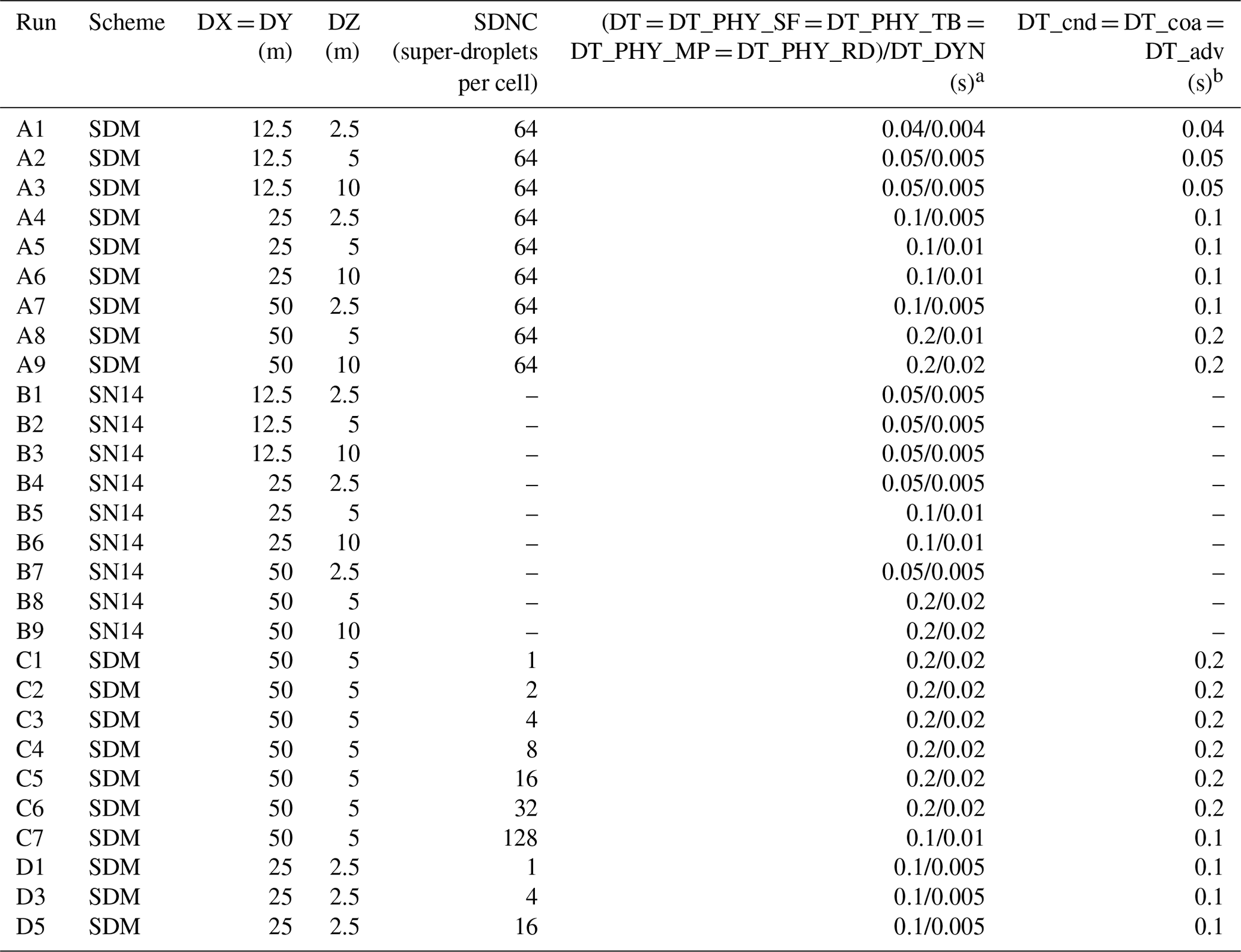
^a DT, DT_DYN, DT_PHY_SF, DT_PHY_TB, DT_PHY_MP, and DT_PHY_RD are the time steps of time integration and dynamical, surface, turbulence, microphysics, and radiation processes, respectively. ^b DT_cnd, DT_coa, and DT_adv are the time steps of the condensation, coalescence, and advection processes, respectively.

The initial vertical profiles of the wind, moisture air, and temperature followed that of Ackerman et al. (2009). The setup was for the model intercomparison project (hereafter, DYCOMS MIP) based on DYCOMS-II (RF02). DYCOMS MIP contained 14 different LES models with bulk or bin microphysics but no LCM. The domain area was 6 km × 6 km × 1.5 km. The simulation time was 6 h. However, due to constraints in computational resources, the simulation with a finer grid resolution of 12.5 m × 12.5 m × 2.5 m conducted using the SDM was limited to 5 h. The periodic boundary condition was imposed for the lateral boundaries. The simplified radiation model described in Ackerman et al. (2009) was used. Unlike in the work of Ackerman et al. (2009), the maximum supersaturation limited to 1 % in the first hour was used herein not only for droplet activation, but also for condensational growth. The initial aerosol number and the size distributions used for the SDM were the bimodal lognormal distribution specified in Ackerman et al. (2009). We reduced the initial aerosol number concentration from 100 to 70 cm⁻³ for the SN14 simulations to make the mean cloud droplet number concentration consistent with that of the DYCOMS MIP (∼ 55 cm⁻³). Constant latent and sensible heat from the surface was imposed. We also slightly decreased the constant surface latent heat flux from 93 to 86.7132 W m⁻² to slightly reduce the predicted liquid water in the SN14 and SDM simulations, thereby avoiding overestimation. The momentum exchange between the super-droplets and the fluid was also considered in the SDM. The SN14 and SDM results were saved every minute.

Table 1 summarizes the specific horizontal and vertical grid lengths, time steps, and SDNC.

1. Grid resolution test (experiment groups A and B).

   Nine different grid resolution settings were used: DX (= DY) × DZ = 50 m × 2.5 m, 50 m × 5 m, 50 m × 10 m, 25 m × 2.5 m, 25 m × 5 m, 25 m × 10 m, 12.5 m × 2.5 m, 12.5 m × 5 m, and 12.5 m × 10 m. The aspect ratio ($\mathrm{DX}/\mathrm{DZ}$) was also considered. All grid cells in the SDM and SN14 runs were uniform and not stretched in space. The SDM and SN14 runs with all different grid spacings were categorized into groups A and B, respectively. In both groups, the runs with DX (= DY) × DZ = 50 m × 5 m were the benchmark runs also used in the DYCOMS MIP. The initial super-droplet number concentrations of the runs in Group A were all 64 per cell. To stabilize the numerical simulations, the time steps were reduced as the resolution became finer. The goal of groups A and B was to explore the grid convergence of SDM and SN14. By comparing these two groups, we expect to find the differences between SDM and SN14.

2. Initial super-droplet number test (experiment groups C and D).

   Eight initial super-droplet number concentrations were set in Group C from smallest to largest: 1, 2, 4, 8, 16, 32, and 128 per cell. The same grid resolutions of the SDM runs in Group C (i.e., 50 m × 5 m) were compared with base run A8. We also investigated the impact of the grid resolution on the super-droplet number characteristics using Group D, which comprised a series of SDM simulations with super-droplet numbers 1, 4, 16, and 64 per cell at a 25 m × 2.5 m resolution. We expected groups C and D to help us understand the super-droplet convergence characteristic of the cloud droplet number concentration (CDNC).

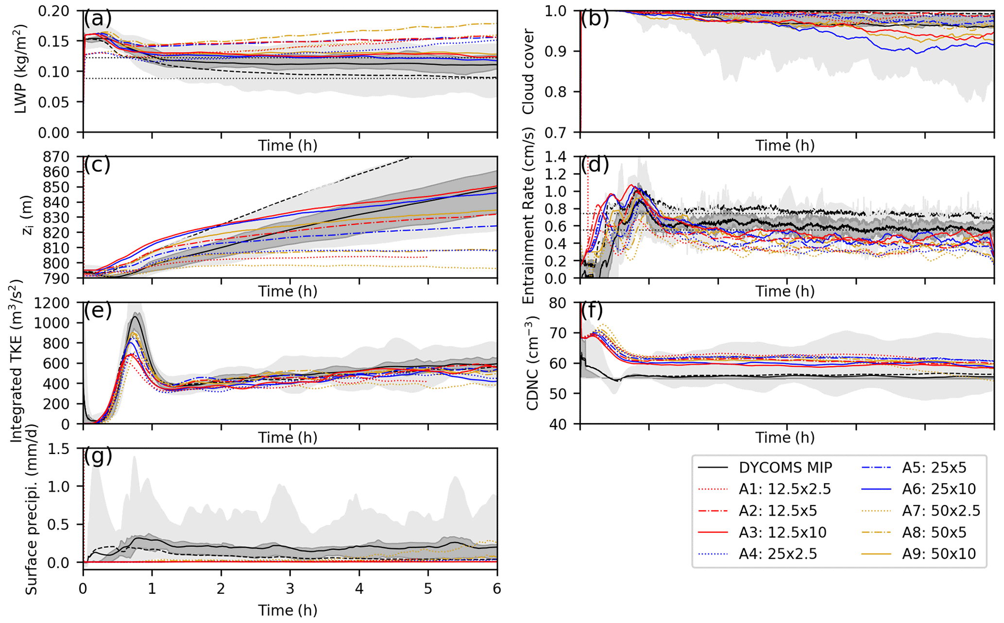
Figure 1 Time series of the (a) liquid water path (LWP), (b) cloud cover, (c) inversion height, (d) entrainment rate, (e) vertically integrated turbulent kinetic energy (TKE), (f) cloud droplet number concentration (CDNC), and (g) surface precipitation for the Group A runs (SDM). The ensemble range, interquartile range, and mean of the DYCOMS MIP results are denoted by the light and dark shading and solid lines, respectively. The ensemble mean from the simulations that included drizzle without sedimentation is denoted by the dashed lines (Ackerman et al., 2009).

3 Numerical convergence characteristics

In this section, we will compare the SCALE results with the DYCOMS MIP results. As specified in the work of Ackerman et al. (2009), the first 2 h was considered as the spin-up period. Moreover, the vertical profiles were averaged over the last 4 h. In all profiles, the y axis is defined as the height normalized by the inversion height z_i, which is the mean height of the q_t = 8 g kg⁻¹ isosurface. The entrainment rate in the simulations was calculated as $E=\frac{\mathrm{d}{z}_{\mathrm{i}}}{\mathrm{d}t}+D{z}_{\mathrm{i}}$, where D = 3.75 × 10⁻⁶ s⁻¹ is the uniform divergence of the large-scale horizontal winds. In the time series and vertical profiles, the ensemble range, interquartile range, and mean of the DYCOMS MIP results are denoted by the light and dark shading and solid lines, respectively. The ensemble mean from the simulations that included drizzle without sedimentation is denoted by the dashed lines (Ackerman et al., 2009).

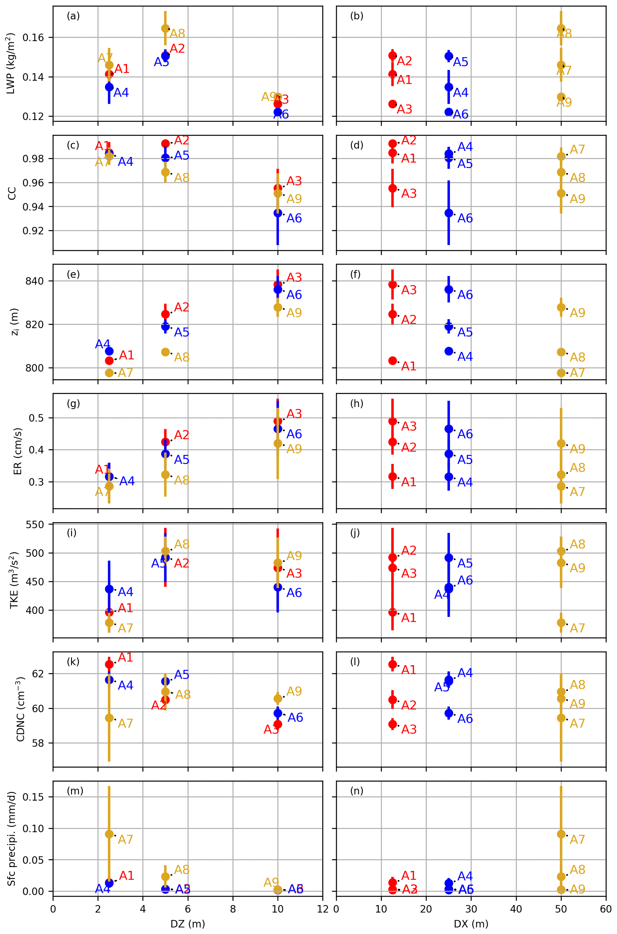
Figure 2 Evolution of the time average of the (a, b) LWP, (c, d) cloud cover, (e, f) inversion height, (g, h) entrainment rate, (i, j) vertically integrated TKE, (k, l) CDNC, and (m, n) surface precipitation for the Group A runs (SDM) with the grid resolution. The left and right columns represent the evolution of the variables with DZ and DX, respectively. Each point in these scatter plots represents the average of one variable from one SDM run. The error bars show the standard deviation of the detrended data.

3.1 SDM grid convergence

In this section, we will analyze the SDM results conducted in various grid resolutions (Group A) to assess the grid convergence characteristics.

3.1.1 Time series of the domain average

Figure 1 shows the time series of several domain-averaged quantities for the SDM results. The results were compared with the DYCOMS MIP results. Figure 2 depicts the statistics of the boundary layer and the cloud-related fields during the last 4 h (the last 3 h for run A1) versus the grid resolutions. The left and right columns represent the change of variables with DZ and DX, respectively. Each point in these plots represents a 4 h average of the variables for the corresponding SDM runs (a 3 h average for run A1). The error bars show the standard deviation of the time series.

The domain-averaged LWP decreased as DZ decreased when DZ ≤ 5 m (Figs. 1a and 2a) and was not very sensitive to DX (Figs. 1a and 2b). The LWP showed the trend of getting closer to the true solution as the grid resolution was being refined; however, the LWP changed rate in terms of DZ remained large, even when DZ = 2.5 m. This indicated that a DZ smaller than 2.5 m (DZ < 2.5 m) was needed to obtain a well-converged solution. We conclude from the LWP time series that DX less than or equal to 50 m (DX ≤ 50 m) was sufficient; however, in the subsequent paragraphs, this conclusion will be proven untrue for all fields. Unlike the DYCOMS MIP, our LWP increased with time in most of our simulations. The LWP values during the last 3 h in our simulations were all larger than the MIP average.

The cloud cover (CC) is the fraction of cloudy columns defined as columns with an LWP larger than 20 g m⁻². Conversely, cloud holes are columns with LWP ≤ 20 g m⁻². Figs. 1b and 2c showed that CC increased as DZ decreased. Its dependency on DX was relatively weak. CC exhibited the trend of getting closer to the true solution as the grid resolution was being refined but was still sensitive to DZ and weakly sensitive to DX, even when (DZ, DX) = (2.5 m, 12.5 m). This may indicate that DZ smaller than 2.5 m (DZ < 2.5 m) and DX smaller than 12.5 m (DX < 12.5 m) are necessary in achieving a converged solution. Our CC results were almost always higher than the MIP ensemble mean, except when DZ = 10 m. CC rapidly declined and deviated from the MIP results when DZ = 10 m.

The inversion height z_i decreased as DZ decreased (Figs. 1c and 2e) and increased as DX decreased except run A1 (Figs. 1c and 2f). z_i displayed the trend of also getting closer to the true solution as the grid resolution was being refined, but remaining strongly sensitive to DZ and weakly sensitive to DX, even when (DZ, DX) = (2.5 m, 12.5 m). In other words, DZ < 2.5 m and DX < 12.5 m are necessary in realizing a converged solution. The differences of z_i among the Group A runs relative to z_i were not big and were less than a few percent. z_i of the SDM rapidly increased during the first 2 h and then flattened, whereas that of the MIP more rapidly and continuously increased. This suggests that the DYCOMS MIP has more instability near the cloud tops, leading to stronger upward wind that promotes cloud top growth, while the SDM has more stable cloud tops.

The entrainment rate (Fig. 1d) slowly decreased in time after the first hour then leveled off. By the definition (Eq. 1) adopted from the DYCOMS MIP, the entrainment rate was determined by the inversion height z_i and its time derivative $\mathrm{d}{z}_{\mathrm{i}}/\mathrm{d}t$. Consequently, its dependency to the grid resolution was similar to that of the inversion height z_i. The entrainment rate decreased as DZ decreased (Fig. 2g) and increased as DX decreased (Fig. 2h). It remained strongly sensitive to DZ and weakly sensitive to DX, indicating that DZ < 2.5 m and DX < 12.5 m are necessary for an accurate simulation. The entrainment rates of the SDM were positioned around the lower end of the DYCOMS MIP range.

The vertically integrated total turbulent kinetic energy (TKE), including the resolved TKE and the SGS TKE, rose rapidly during the first 40 min and then fell sharply and rose slowly after the first hour (Fig. 1e). It was insensitive to DX (Figs. 1e and 2j) and DZ (Figs. 1e and 2i). Therefore, DZ < 2.5 m and DX ≤ 50 m are necessary for an accurate simulation. For all the SDM runs, the vertically integrated TKE was almost always around the MIP ensemble average.

The CDNC (Fig. 1f) rapidly decreased in the first hour, with an average value of approximately 60 cm⁻³, which was slightly higher than the MIP ensemble average (∼ 55 cm⁻³). It was sensitive to DZ (Figs. 1f and 2k), but its dependence on it is unknown and less sensitive to DX (Figs. 1f and 2l). Therefore, DZ < 2.5 m and DX ≤ 50 m are necessary for an accurate simulation.

The surface precipitation (Fig. 1g) in all our simulations was much lower than that in the DYCOMS MIP. Although our SDM results greatly differed from bulk and bin microphysics of the DYCOMS MIP, they were consistent with those in the previous SDM study on this case by Dziekan et al. (2019). Figure 2m illustrates the surface precipitation increase with the decreasing DZ. However, its dependency on DX was not clear, whereas run A7 has the heaviest surface precipitation of all simulations (Fig. 2n).

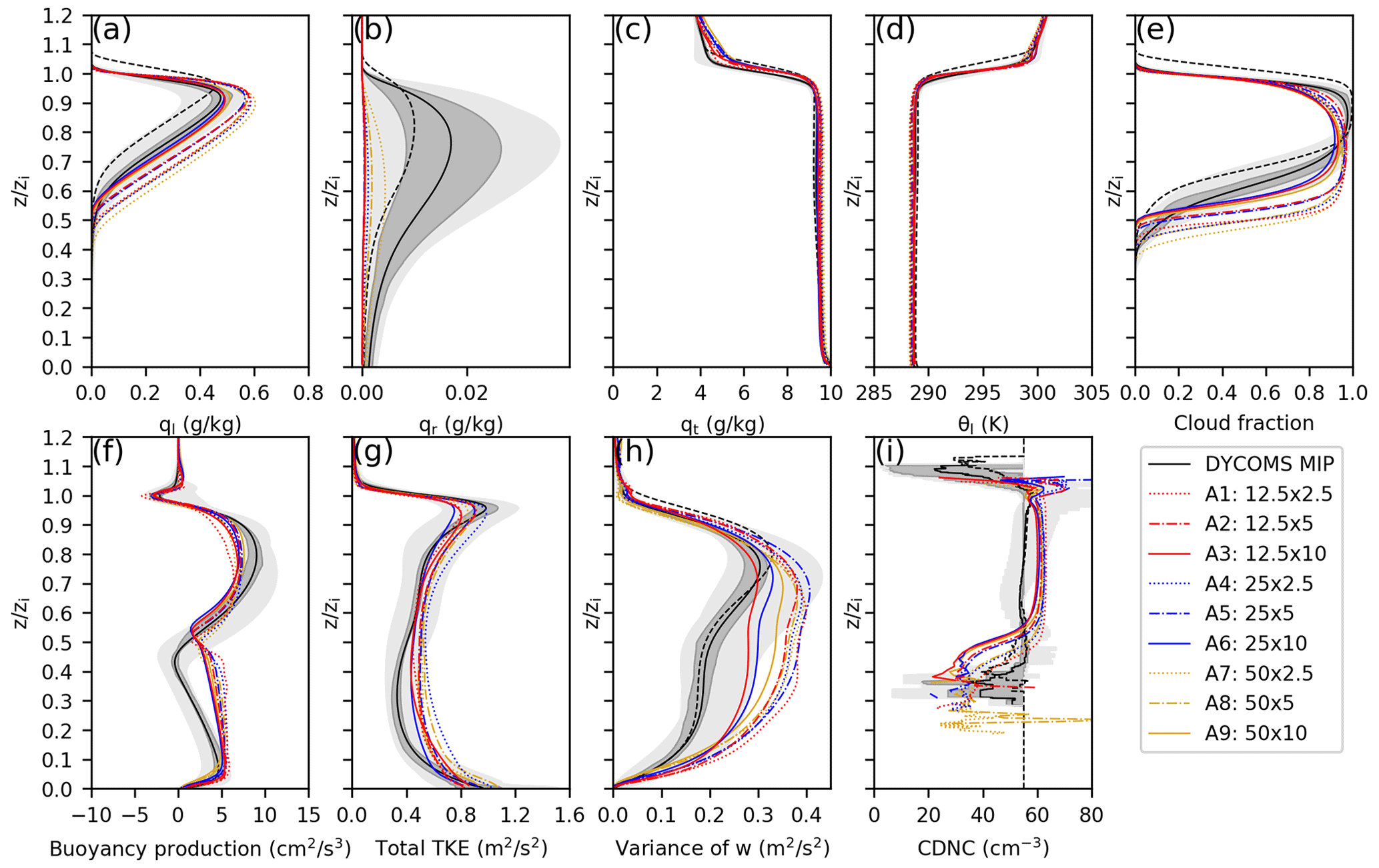
Figure 3 Vertical profiles of the (a) liquid water mixing ratio, (b) rain water mixing ratio, (c) total water mixing ratio, (d) liquid water potential temperature, (e) cloud fraction, (f) buoyancy production, (g) total TKE, (h) w variance (variance of the vertical wind speed), and (i) CDNC for the Group A runs (SDM). The meanings of light and dark shading, solid lines, and dashed lines are the same as in Fig. 1.

3.1.2 Horizontally averaged vertical profile

In addition to the time series in Figs. 1 and 2, we further investigated the vertical profiles to examine the grid convergence and the vertical structure of clouds. Figure 3 depicts the vertical profiles obtained by the horizontal average during the last 4 h (a 3 h average for run A1). The vertical axis in these plots represents the real height z scaled by the inversion height z_i.

The liquid water potential temperature θ_l (Fig. 3d) and the total water mixing ratio q_t (Fig. 3c) were not sensitive to the grid resolution. Consistent with the surface precipitation time series (Fig. 3g), the rain water mixing ratio q_r profile (Fig. 3b) was almost 0.

The liquid water mixing ratio q_l (Fig. 3a) increased as DZ decreased and was not sensitive to DX. It remained strongly sensitive to DZ; hence, (DZ ≪ 2.5 m ∧ DX ≤ 50 m) is necessary for an accurate simulation.

Figure 4 Horizontal LWP distribution at 200 min in Series A (SDM). The size of the cloud holes decreased when the resolution became finer.

Figure 3e showed the cloud fraction (CF; fraction of the cloudy grid cells defined as the grid cells with CDNC > 20 cm⁻³). CF in the lower part of the cloud deck depicted the same grid resolution dependency as q_l. The lower-part CF increased as DZ decreased. When DZ = 2.5 m, the lower-part CF increased with decreasing DX but was strongly sensitive to DZ. In other words, (DZ ≪ 2.5 m ∧ DX < 12.5 m) is needed for the lower-part CF. Conversely, when examining the CF profile around its peak within the cloud deck's midsection, the characteristics of grid convergence were ambiguous. The peak CF values were very similar across simulations with DZ ≤ 5 m. In short, (DZ ≪ 2.5 m ∧ DX < 12.5 m) is necessary for the accurate simulation of the CF. CF in all SDM runs was smaller in the upper part of the cloud deck but larger in the lower part of the cloud deck than that in the DYCOMS MIP. Figure 4 showed the horizontal LWP distribution at the end of the simulation (t = 200 min). Some cloud holes (areas with very low LWP) could be found in Group A. These cloud holes shrank as the grid resolution increased. Figure 3i presented the averaged CDNC profiles exclusively within cloudy cells, revealing an inverse correlation where the CDNC escalates with a decrease in DZ.

The TKE profiles (Fig. 3g) and the variance of the vertical velocity profiles (Fig. 3h) were almost within the ensemble range of the DYCOMS MIP in the cloud deck. Their grid dependency was similar to that of the vertically integrated TKE time series. The TKE profile increased as DZ decreased. It was less sensitive to DX, but stayed strongly sensitive to DZ. Hence, (DZ ≪ 2.5 m ∧ DX ≤ 50 m) is necessary for an accurate simulation.

The TKE buoyancy production profile (Fig. 3f) was relatively insensitive to the grid resolution in the upper part of the cloud layer. We could find a similar dependency to the TKE profiles (Fig. 3g) in the region around the cloud base (i.e., lower part of the cloud and sub-cloud layers). It increased as DZ decreased and was insensitive to DX. Considering the grid dependencies of the two regions, (DZ ≪ 2.5 m ∧ DX ≤ 50 m) is necessary for an accurate simulation. Note also that in the SDM, the buoyancy production below the cloud base is much bigger than that in the DYCOMS MIP.

3.1.3 Summary of the SDM grid convergence and interpretation

Based on the Group A results presented in Figs. 1–4, the results were qualitatively comparable with each other and got closer to the true solution as the grid resolution was being refined. However, the (DZ, DX) = (2.5 m, 12.5 m) resolution was not high enough yet. In particular, the result was still strongly sensitive to DZ.

Putting everything together, a much finer vertical resolution (DZ ≪ 2.5 m) is necessary for almost all quantities. A finer horizontal resolution (DX < 12.5 m) is necessary for CC, CF, z_i, and entrainment rate.

We interpret the DZ dependency here. A more detailed cloud structure can be resolved when DZ is refined. This results in a higher CC (Figs. 1b and 4) and an enhanced cloud top cooling. The cooler boundary layer confirmed from the enlarged θ_l profile (not shown) led to a higher CF (Fig. 3e). Focusing on the lower part of the cloud layer (just above the cloud base) in Fig. 3e, we can observe a relatively large discrepancy of the CF between runs with DZ = 2.5 m and those with DZ = 10 m, explaining the difference of the q_l profiles (Fig. 3a). The larger cloudy area near the cloud base resulted in a stronger TKE buoyancy production in the higher-resolution runs (Fig. 3f). In the marine stratocumulus case, the contribution of the buoyancy production dominated the TKE, consequently increasing the TKE (Fig. 3g) and developing the cloud structure that can be confirmed by the higher LWP in the time series (Fig. 1a) and thicker cloud layer (Fig. 3e).

3.2 Super-droplet number convergence

The super-droplet number convergence is discussed in this section. The SDM results at 50 m × 5 m with different initial super-droplet numbers ranging from 1 to 128 super-droplets per cell were compared (Group C). A similar comparison with a finer grid resolution of 25 m × 2.5 m (Group D) was also performed to determine the impact of the grid size on the super-droplet number convergence characteristics.

Figure 5 Evolution of the time average of the (a) LWP, (b) cloud cover, (c) inversion height, (d) entrainment rate, (e) vertically integrated TKE, (f) CDNC, and (g) surface precipitation for the Group C and D runs and runs A8 and A4 with the SDNC. Each point in these scatter plots represents the average of one of those variables from one SDM run. Group C and D are marked in by a circle and x, respectively. The error bars show the standard deviation of the detrended data.

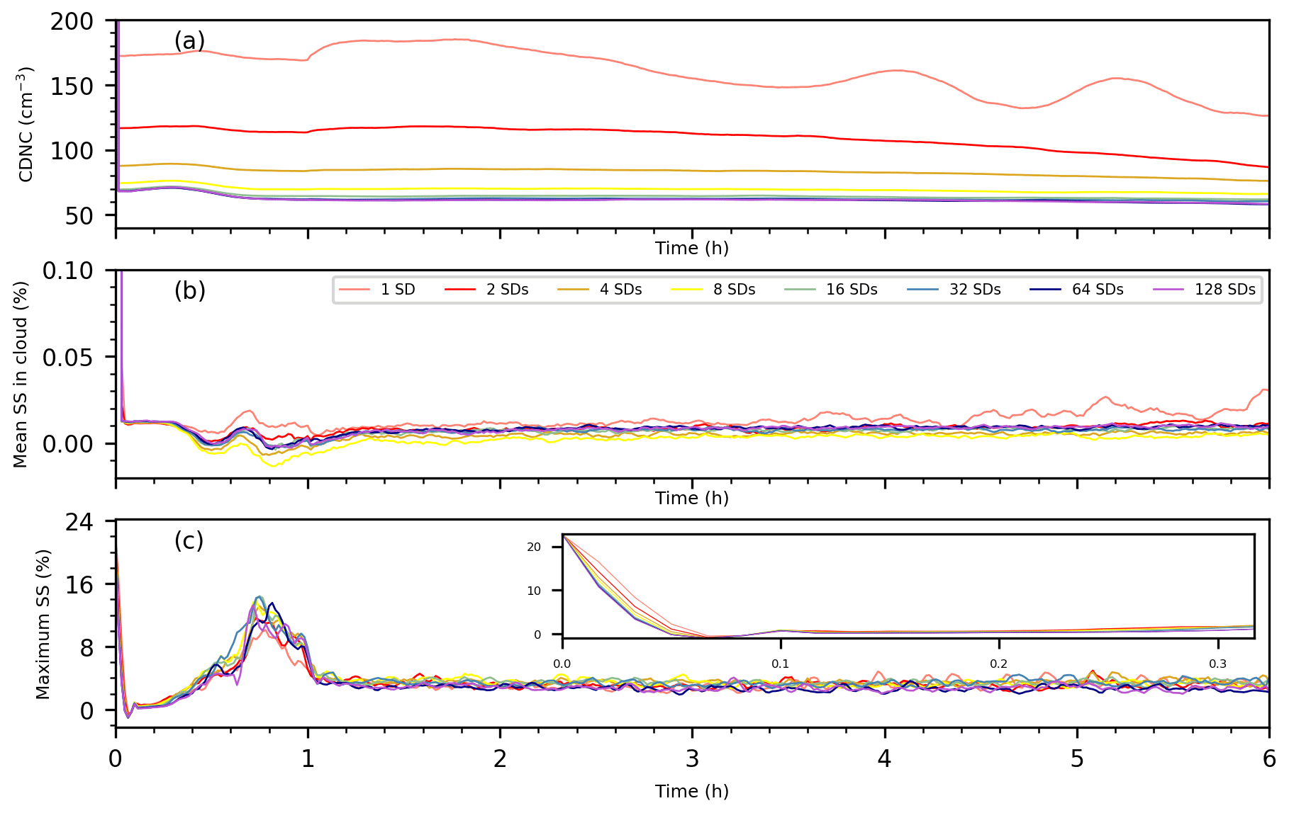
Figure 6 The time series of (a) CDNC, (b) mean supersaturation within cloudy cells, and (c) maximum supersaturation for the SDM simulations with diverse initial super-droplet (SD) concentrations (Group C), conducted at a grid resolution of 50 m × 50 m × 5 m. Notably, the inset in panel (c) accentuates the first 20 min, underlining the inversely proportional relationship observed between initial super-droplet number concentrations and the magnitude of maximum supersaturation.

Figure 5 depicts the last 4 h average of the variables versus the initial super-droplet number concentration. In Group C, CDNC and precipitation decreased, and the entrainment rate and the inversion height increased with the increasing super-droplet number. CDNC converged to approximately 60 cm⁻³. All the SDM results converged well in addition to the LWP and z_i when the initial SDNC was greater than or equal to 16 per cell. The absolute relative errors between C5 (16 per cell) and C7 (128 per cell) in CC, z_i, TKE, and CDNC were smaller than 5 %. We proposed herein an explanation for the CDNC decrease with the increasing SDNC (Figs. 5f and 6a). In a case with a quite small initial SDNC (e.g., 1 or 2 super-droplets per cell on average), the multiplicity of super-droplets may therefore be very high, and the phase relaxation time may be very long in some grids with almost no super-droplets and become extremely short in grids with relatively many super-droplets. Consequently, there is a greater potential for greater supersaturation, and thus more aerosols are activated to the cloud droplets. The time evolution of the supersaturation supports our point: the maximum supersaturation (Fig. 6c) significantly decreases as the SDNC increases during the beginning of the simulations. When the SDNC is small (e.g., 1 or 2), the average supersaturation in the cloudy grids (Fig. 6b) is also essentially at a relatively high value.

The variables in Group D (higher grid resolution) showed the same trend with the SDNC as those in Group C (lower grid resolution). The results in the high-resolution runs also converged well when CDNC ≥ 16 per cell. The absolute relative errors between D5 (16 per cell) and A4 (64 per cell) in the LWP, CC, z_i, entrainment rate, CDNC, and surface precipitation were smaller than 5 %.

It is worth noting that for cases with large amounts of precipitation formation, a low super-droplet number per grid may not be sufficient. This may affect the precipitation formation rate and the spatial distribution of rain and cloud water. Similarly, for polluted cases with GCCN (giant CCN), a sufficient number of super-droplets may be needed to properly sample the aerosol size spectrum and capture the effect of GCCN on precipitation initiation. Dziekan et al. (2021) found that the addition of GCCN to the SDM simulation can significantly increase the precipitation of stratocumulus.

In general, the SDM results all converged well at the initial SDNC greater than or equal to 16 per cell. All, except precipitation, were within the ensemble range of the DYCOMS MIP. The comparison study on different grid resolution indicated that the super-droplet number per grid cell, not per unit volume, is essential for the super-droplet number convergence characteristic. Considering the balance of the computational cost and the simulation accuracy, the SDNC of 16 per cell is the optimal choice of the SDM for the stratocumulus simulations.

Figure 7 Time series of the (a) LWP, (b) cloud cover, (c) inversion height, (d) entrainment rate, (e) vertically integrated TKE, (f) CDNC, and (g) surface precipitation for the Group B runs (SN14). The meanings of light and dark shading, solid lines, and dashed lines are the same as in Fig. 1.

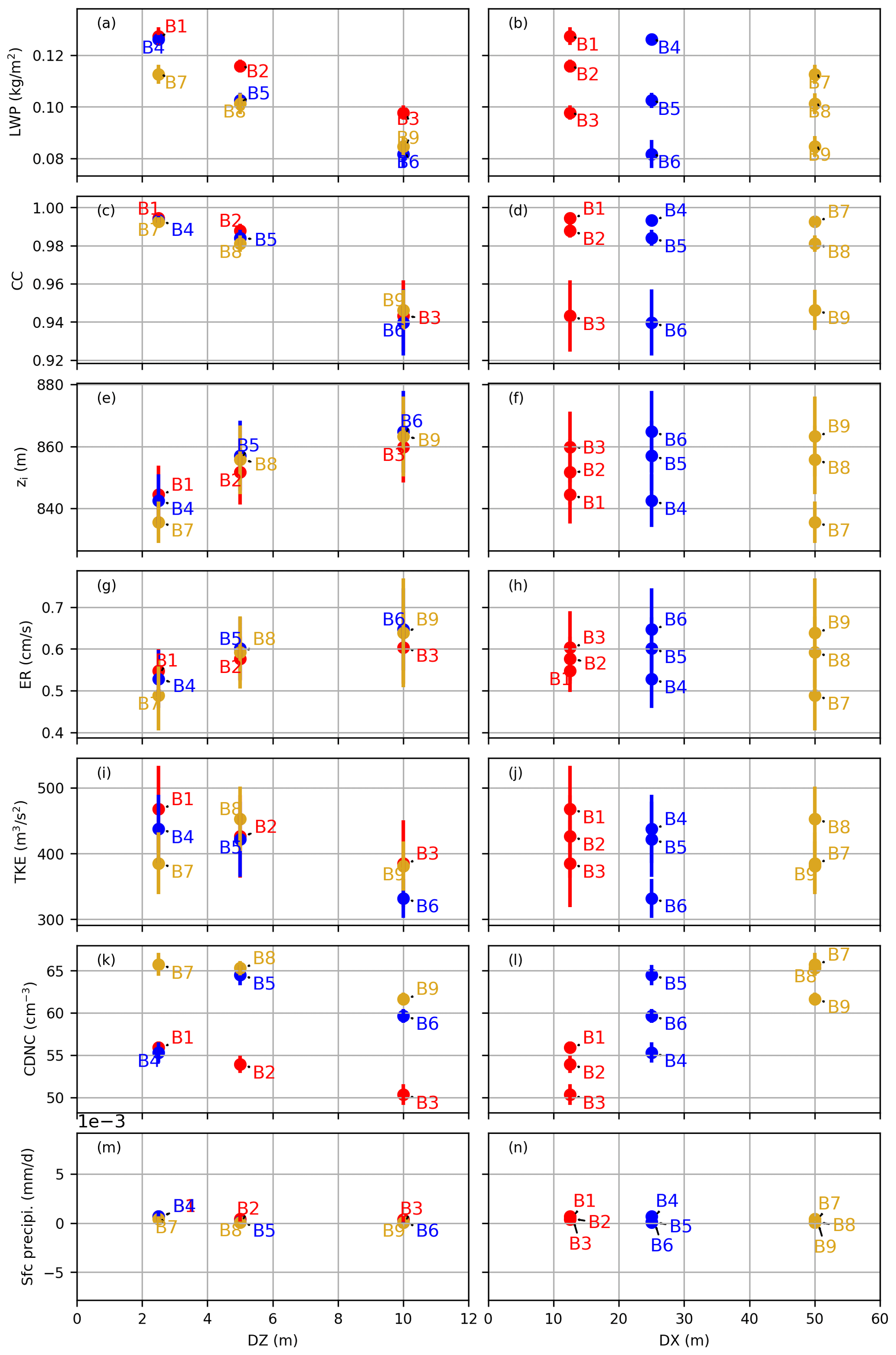
Figure 8 Evolution of the time average of the (a, b) LWP, (c, d) cloud cover, (e, f) inversion height, (g, h) entrainment rate, (i, j) vertically integrated TKE, and (k, l) CDNC and (m, n) surface precipitation for Group B runs (SN14) with the grid resolution. The left and right columns represent the evolution of the variables with DZ and DX, respectively. Each point in these scatter plots represents the average of one of the variables from one SN14 run. The error bars show the standard deviation of the detrended data.

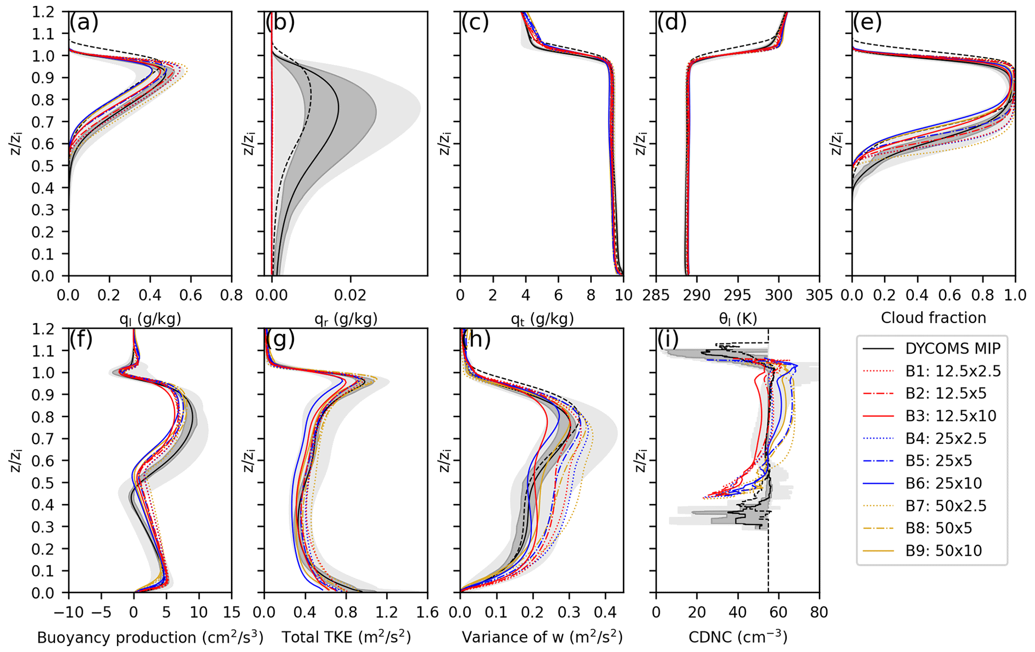
Figure 9 Vertical profiles of the (a) liquid water mixing ratio, (b) rain water mixing ratio, (c) total water mixing ratio, (d) liquid water potential temperature, (e) cloud fraction, (f) buoyancy production, (g) total TKE, (h) w variance, and (i) CDNC for the Group B runs (SN14). The meanings of light and dark shading, solid lines, and dashed lines are the same as in Fig. 1.

3.3 SN14 grid convergence

Similar to Sect. 3.1 for the SDM, this section discusses the conducted SN14 simulations in various grid resolutions (Group B) and the investigated grid convergence characteristics. The time series (Figs. 7 and 8) and the vertical profiles (Fig. 9) of Group B are shown.

The LWP (Figs. 7a and 8a), q_l (Fig. 9a), and lower-part CF (Fig. 9e) depicted a similar dependency on the grid spacings; that is, they increased as DZ decreased. The dependency on DX was unclear (Fig. 8b). B1 (12.5 m × 2.5 m) and B4 (25 m × 2.5 m) were indistinguishable. In other words, (DZ ≪ 2.5 m ∧ DX ≤ 25 m) is necessary for these variables. The cloud deck of SN14 was thicker than that of the SDM. Consequently, it contained more liquid water. SN14 agreed with the MIP better than the SDM.

Figure 10 Horizontal LWP distribution at 200 min in Series B (SN14).

Accordingly, CC (Figs. 7b and 8c) and maximum CF (Fig. 9e) showed similar dependencies to the grid spacings; that is, they increased as DZ decreased (Fig. 8d) but were not sensitive to the grid spacings if (DZ ≤ 5 m ∧ DX ≤ 50 m). CC and maximum CF of SN14 were nearly one, a reflection of minimal cloud holes as evidenced by the horizontal distribution of LWP observed in Figs. 4 and 10. This near-unity in CC and peak CF is indicative of a highly continuous cloud field.

Similar to the result in the SDM, the inversion height z_i (Figs. 7c and 8e) decreased as DZ decreased (Fig. 8f). The DX dependency was unclear, but for all DZ, DX = 25 m and DX = 12.5 m agreed well, indicating that (DZ ≪ 2.5 m ∧ DX ≤ 25 m) is necessary for an accurate simulation. The entrainment rate (Figs. 7d and 8g, h) was determined by z_i and $\mathrm{d}{z}_{\mathrm{i}}/\mathrm{d}t$. z_i and the entrainment rate of SN14 were larger than those of the SDM due to the fast increase in z_i during the spin-up time period. z_i of SN14 was located around the upper end of the MIP, but the entrainment rate of SN14 during the last 4 h agreed well with the MIP result.

The TKE (Figs. 7e, 8i, and 9g), w variance (Fig. 9h), buoyancy production around the cloud base (Fig. 9f), and CDNC (Figs. 7f, 8k, and 9i) showed similar dependencies; that is, they increased as DZ decreased and decreased as DX decreased. In other words, (DZ ≪ 2.5 m ∧ DX ≤ 25 m) is necessary for an accurate simulation. No clear trend was observed in the grid dependency of the buoyancy production near the cloud top, but B1 (12.5 m × 2.5 m) and B4 (25 m × 2.5 m) were almost indistinguishable.

All variables characterizing turbulence (i.e., TKE, w variance, and buoyancy production) were larger in SN14 than in the SDM. In particular, the buoyancy production in the cloud layer was noticeably higher in SN14 than in the SDM. SN14 agreed better with the MIP.

The surface precipitation and q_r were so small in all the Group B results that they did not affect the overall grid convergence characteristics. This was in agreement with the SDM results but much lower than the ensemble mean of the MIP.

SN14 showed a higher CDNC than the SDM in the first hour and a lower CDNC during the last 5 h (Figs. 1f and 7f). The higher peak of the CDNC in SN14 might be caused by the higher maximum supersaturation during the first hour. In that of Ackerman et al. (2009) and our SDM simulation, the maximum supersaturation was limited to 1 % during the convection spin-up to avoid precipitation suppression, which was not adapted in our SN14 simulation. We conducted an SN14 sensitivity test with the supersaturation limiter. The result (not shown) showed a lower CDNC during the first hour (maximum reduced from 120 to 90 cm⁻³), but it had little effect on the CDNC after the spin-up stage.

From Figs. 7–9, we conclude that the LWP, q_l, CC, CF, TKE, w variance, and buoyancy production around the cloud base and CDNC increased, and the inversion height and the entrainment rate decreased with the decreasing DZ. However, the grid dependency on DX was relatively weak. The sensitivity of the variables to the grid resolution in SN14 was very similar to that in the SDM, but the SDM variables showed a stronger grid dependency on DZ and DX. In conclusion, the variation trend of the variables with the grid resolution in SN14 was more ambiguous than that in the SDM.

In summary, a much finer vertical resolution (DZ ≪ 2.5 m) was necessary for almost all quantities, except for CC and maximum CF. The horizontal resolution of DX = 25 m was sufficient for all quantities. The SN14 results agreed with the MIP better than the SDM results.

3.4 Summary of the numerical convergence characteristics

Section 3.1 and 3.3 revealed the grid convergence characteristics of SDM and SN14, respectively. The finest grid resolution tested was (DZ, DX) = (2.5 m, 12.5 m). Our analysis revealed that the grid convergence of both schemes has not yet been achieved. However, we observed a trend where the results approached the true solution. Overall, under the tested parameter range, both SDM and SN14 were strongly sensitive to the vertical resolution and relatively weakly sensitive to the horizontal resolution.

In conclusion, DZ ≪ 2.5 m was necessary for both schemes. Note, however, that the TKE and CDNC in the SDM and the CC and the maximum CF in SN14 were not any more sensitive to DZ.

In the SDM, a finer horizontal resolution (DX < 12.5 m) was necessary for CC, maximum CF, z_i, and entrainment rate. In contrast, the horizontal resolution of DX ≤ 25 m was sufficient for SN14.

Figure 11 Time series of the LWP, cloud cover, inversion height, entrainment rate, vertically integrated TKE, CDNC, and surface precipitation for runs A8, B8, and SDM without sedimentation and SDM with horizontal SGS turbulent mixing.

This grid convergence characteristic study showed that when the aspect ratio is unchanged, the LWP increases with the decreasing grid spacing, consistent with the previous studies (Pedersen et al., 2016; Mellado et al., 2018; Matheou and Teixeira, 2019) with isotopic grids (DX/DZ = 1). Some studies on the role of the grid resolution in the numerical simulations of the turbulent entrainment have also shown that the accurate entrainment rate simulation requires a vertical grid spacing no greater than the turbulent undulation scale, which can be 5–10 m for the inversion and turbulence levels typical of the subtropical marine stratocumulus (Stevens and Bretherton, 1999).

However, the stratocumulus simulation is notorious for such a slow grid convergence with respect to the vertical grid spacing DZ. The LES study of Matheou and Teixeira (2019) showed that the numerical convergence for the LWP is hard to achieve, even if the isotopic grid size of 1.25 m is used. However, the LES utilizing a 1.25 m grid resolution can reproduce a detailed cloud structure (e.g., elongated regions of low LWP, cloud holes, and pockets) (Matheou, 2018). Mellado et al. (2018) suggested that 2.5 m or less was necessary for their LES to approach the observation. Furthermore, the LWP was numerically converged when the Kolmogorov scale used in their direct numerical simulation (DNS), which was smaller than 0.7 m.

In Sect. 3.2, we also conducted a numerical convergence analysis on the super-droplet numbers at different grid resolutions. In conclusion, the initial super-droplet number concentration ≥ 16 per cell is sufficient for the tested stratocumulus case. The super-droplet number convergence characteristic was essentially determined by the super-droplet number per grid cell and not per unit volume. The LWP, CC, inversion height, entrainment rate, and TKE results also supported the finding that SDNC ≥ 16 per cell was good enough for an accurate stratocumulus simulation.

Note also that the SN14 results agreed with the MIP better than the SDM results. In the subsequent sections, we will focus on understanding the difference in the SDM, SN14, and MIP and conduct an in-depth analysis to elucidate the underlying mechanism.

4 Comparison of the SDM and SN14

In Sect. 3, we explored grid convergence characteristics of the SDM and SN14, noting their similar dependencies on grid size yet distinct outcomes in the cloud top height, entrainment rate, liquid water content, CF, CDNC, and turbulence characteristics.

Figure 12 Vertical profiles of the (a) liquid water mixing ratio, (b) rain water mixing ratio, (c) total water mixing ratio, (d) liquid water potential temperature, (e) cloud fraction, (f) buoyancy production, (g) total TKE, (h) w variance, and (i) CDNC for the A8, B8, and SDM without sedimentation and SDM with horizontal SGS turbulent mixing.

The SDM simulations consistently yielded higher LWP values that exhibited an upward trend, unlike the SN14 simulations where LWP appeared lower and remained relatively constant past the initial hour (Fig. 11a). Furthermore, the SDM predicted enhanced q_l (Fig. 12a) and a denser cloud base, evidenced by an increased cloud fraction near the cloud base, in contrast to the SN14 scheme which indicated a propensity towards more pronounced vertical cloud development, as demonstrated by a larger maximum cloud fraction near the cloud top (Fig. 12e).

The differences between the SDM and SN14 may stem from their distinct aerosol treatment, which caused the difference between SDM and SN14. Temporal changes of aerosol size distribution through wet deposition were explicitly considered in the SDM, while background aerosol particles were assumed to be uniform and unchanged in SN14. Considering the 6 h simulation time, this could modulate the characteristics of the stratocumulus deck.

Figure 13 Vertical profiles of q_l, q_r, q_t, θ_l, buoyancy production, total TKE, N_c, N_p, q_n, N_SD, CF, and N_c for runs A8 and SDM without sedimentation. The solid and dashed lines in panels (a)–(j) represent the profiles in the cloudy and hole columns, respectively.

To examine our hypothesis concerning aerosol wet deposition through cloud droplet sedimentation, an SDM simulation without sedimentation (SDM_no_sed) was conducted. In this simulation, all super-droplets are treated as passive tracers when updating their positions; i.e., their terminal velocities are always zero. Note also that their collision–coalescence by differential sedimentation is still considered in SDM_no_sed. The vertical profiles of the total particle number concentration N_p, total particle number mixing ratio q_n (ratio of N_p and air density), and super-droplet number concentration N_SD in the SDM simulations reveal local minima near the cloud top, consistent across scenarios with and without sedimentation (illustrated in Fig. 13h, i, and j, respectively). Notably, these minima were more pronounced in the simulations incorporating the sedimentation process, aligning with our conjecture and underscoring the sedimentation's significant impact on particle distribution near the cloud top. This aerosol particle depletion near the cloud top propagated to the hole volume (Fig. 13h, i, and j). Moreover, the aerosol particle depletion in the hole volume in the SDM would make the cloud hole persistent (Fig. 13k). Note also that Fig. 9b of Arabas et al. (2015) also showed the depletion of aerosol particles near the stratocumulus top and the associated hole volume. On the other hand, relatively high concentrations of particles near the cloud top with almost no cloud holes could be found in SDM_no_sed (Fig. 13h, i, j, and k). The above results demonstrated that the wet deposition of aerosols was responsible for the low CF near the cloud top and it also lowered the cloud tops of marine stratocumulus clouds and increased the cloud fraction near the cloud base. In our simulations, we assumed that the aerosol number concentration was initially uniform in space, including the free atmosphere. This should partially compensate for the aerosol particle reduction at the cloud top. In other words, the effect of the cloud top aerosol reduction on the cloud top volume reduction should be greater in the real world. Another Lagrangian cloud model, called UWLCM (Dziekan et al., 2019), presented a similar CF profile to ours in this stratocumulus case. Since all the super-droplets in SDM_no_sed do not sediment, larger droplets within the cloud are more prone to collide and coalesce. Consequently, cloud droplets are more likely to be collected in SDM_no_sed. This leads to an increase in q_r (Fig. 13b) and a decrease in CDNC (Fig. 13i).

The underlying reasons for these discrepancies could also be attributed to the inherent modeling capabilities and approaches of the SDM and SN14. The SDM's design to circumvent numerical diffusion issues enables it to avoid the unphysical dispersion of moisture and cloud droplets across space. Consequently, cloud droplets were not artificially diffused into dry air to evaporate; instead, localized areas of higher supersaturation promote more water vapor to condense onto cloud droplets, leading to an increased liquid water content. This enhanced liquid water content further intensified radiative warming at the cloud base and radiative cooling at the cloud top. Radiative warming at the cloud base potentially made the airflows near the cloud base more active, thereby increasing TKE and facilitating more moisture transport into the cloud. As a result, in the SDM simulations, the cloud fraction, liquid water mixing ratio, buoyancy production, and CDNC were relatively higher near the cloud base (Fig. 12). Stronger radiative cooling at the cloud top reduced the temperature in this region (Fig. 12d), enhancing the stability of the cloud top, which in turn diminished cloud top entrainment mixing (Fig. 11d) and TKE (Fig. 11e). The localized subsidence that ensued acts to suppress the vertical development of the cloud layer, evidenced by a reduced cloud top height (Fig. 11c) and buoyancy production at the cloud top (Fig. 12f), leading to a decrease in CF near the cloud top (Fig. 12e).

Although the avoidance of numerical diffusion is hypothesized to contribute to the enhanced liquid water content observed in SDM simulations, the precise impact of numerical diffusion on cloud dynamics necessitates further exploration. Subsequent sensitivity experiments are imperative to rigorously evaluate the extent of numerical diffusion's influence and to corroborate the mechanisms suggested by this study.

In addition to aerosol wet deposition and numerical diffusion effects, the treatment differences in CCN activation–deactivation between the SDM and SN14 may also have influenced the simulation outcomes. The nucleation scheme in SN14 potentially induces more frequent activation–deactivation events compared to the explicit calculations in SDM, possibly affecting latent heat exchange and cloud droplet formation (Hoffmann, 2016; Yang et al., 2023). This aspect of model divergence also requires additional investigation to substantiate its effects on buoyancy flux and cloud structure.

From the simulations presented herein, we could not conclude which mechanism is dominating the phenomenon. A detailed assessment of the proposed scenarios will be conducted in future studies.

5 Conclusions

In this study, we assessed the performance of the Lagrangian particle-based cloud microphysics scheme, called SDM, for the marine stratocumulus simulation. To do this, we conducted a series of numerical simulations based on DYCOMS-II (RF02). For comparison, we also tested a double-moment bulk scheme, called SN14, using the same dynamical core.

Our simulation results were compared with the results of the model intercomparison project DYCOMS-II (RF02) MIP (Ackerman et al., 2009). In general, all the SDM and SN14 variables mostly showed a reasonable agreement with the MIP results.

We also investigated the numerical convergence characteristics of both schemes. We first assessed their grid convergence and confirmed their similar grid size dependencies. The stratocumulus cloud simulation was more sensitive to the vertical resolution than the horizontal resolution. Both SDM and SN14 simulations showed that as DZ decreased, there was an increase in CC, q_l, TKE, w variance, CDNC, CF, and buoyancy production near the cloud base. Conversely, the inversion height (z_i) and the entrainment rate decreased with decreasing DZ. It is noteworthy that the LWP exhibited distinct sensitivities to DZ in the two schemes: in the SDM, the LWP decreased as DZ diminishes, particularly when DZ ≤ 5 m; conversely, in the SN14, the LWP increased with a decrease in DZ. Despite refining the grid resolution, these variables had not converged within the assessed grid spacing range, indicating that a DZ smaller than 2.5 m may be necessary for a well-converged solution. However, CC, CF, LWP, and q_l appeared to be relatively insensitive to changes in DX. The previous studies suggested that an isotopic grid size of 2.5 m or less is needed for the LES (Mellado et al., 2018). Conclusively, DZ ≪ 2.5 m was necessary for both SDM and SN14, DX < 12.5 m was necessary for the SDM simulations, and DX ≤ 25 m was sufficient for SN14. Considering the huge computational resources required, we could not conduct in-depth and finer-resolution simulations to explore the grid size convergence properties of the SDM and SN14.

According to the super-droplet convergence results, the CDNC increased with the decreasing SDNC due to the longer phase relaxation time. The simulations numerically converged when the SDNC was larger than 16 super-droplets per cell, which is smaller than the 40 super-droplets per cell that Dziekan et al. (2019) confirmed. The entrainment rate and the inversion height also increased with the increasing SDNC. The super-droplet convergence study on different grid resolutions indicated that the super-droplet number per grid cell was more essential for the SDM simulation than that per unit volume. Considering the balance of the computational cost and the simulation accuracy, the SDNC of 16 per cell is the optimal choice of the SDM for this marine stratocumulus case.

In conclusion, our results suggest that due to the difficulty of the grid convergence of the cloud liquid, finer resolutions, especially vertical ones, are necessary for stratocumulus simulations using the SDM and the bulk scheme. Accordingly, to improve the computational efficiency, 16 super-droplets per grid cell should be enough for the SDM simulation of non-precipitating marine stratocumulus cases. When computational resources are limited, utilizing stretched grids can be beneficial. As mentioned previously, for simulating stratocumulus clouds, the liquid-water-related variables (e.g., LWP, CC, CF) exhibit a stronger dependence on vertical resolution than horizontal resolution. Therefore, it is possible to allocate a finer vertical resolution in the boundary layer while maintaining a coarser resolution in the free atmosphere to conserve computational resources. Additionally, some studies have highlighted the presence of a very thin inversion structure due to strong radiative cooling at the top of stratocumulus clouds, and turbulent entrainment through this thin layer can exert significant feedback effects on boundary layer and cloud properties (Mellado et al., 2018). Consequently, it is advisable to maintain a fine vertical resolution near the cloud top.

The main discrepancies between the SDM and SN14 simulations of marine stratocumulus are reflected in the content and distribution of liquid water as well as in the macrostructure of the cloud. The SDM simulations consistently yielded higher LWP values that increased over time, contrasting with SN14 simulations, where LWP remained lower and relatively stable past the initial hour. SDM predicted enhanced q_l and a denser cloud base, evidenced by an increased CF near the cloud base. Conversely, SN14 tended towards more vertical cloud development, as shown by a larger maximum CF near the cloud top.

The differences observed between the SDM and SN14 simulations can be attributed to their distinct aerosol treatment. In the SDM approach, the dynamic process of aerosol size distribution through wet deposition is actively modeled, allowing for a realistic representation of aerosol behavior over time. Conversely, the SN14 scheme employs a static approach, treating background aerosol particles as constant and uniform throughout the simulation. This fundamental difference in aerosol treatment between the two models has the potential to significantly influence the behavior and structure of stratocumulus clouds over the course of a 6 h simulation period. The total particle number concentration N_p, total particle number mixing ratio q_n (ratio of N_p and air density), and super-droplet number concentration N_SD exhibit local minima near the cloud tops in simulations with and without the inclusion of sedimentation processes (SDM and SDM_no_sed, respectively). These minima are accentuated in simulations incorporating sedimentation, highlighting its significant role in altering particle distributions near the cloud top. Furthermore, aerosol depletion within the hole volume in SDM simulations promotes the persistence of these holes, contrasting with the SDM_no_sed scenario, where a higher particle concentration near cloud tops and a virtual absence of the hole volume are observed. This indicates wet deposition's pivotal role in reducing CF near the cloud top, lowering the cloud top, and enhancing CF near the cloud base in marine stratocumulus clouds.

The discrepancies noted could be attributed to the inherent modeling capabilities and methodologies of the SDM and SN14. Specifically, the SDM's strategy to evade numerical diffusion issues allows it to prevent the unphysical spread of moisture and cloud droplets. This characteristic facilitates the formation of localized regions of enhanced supersaturation, promoting the condensation of water vapor into cloud droplets. It concurrently minimizes the dispersion of cloud droplets into unsaturated areas, thereby mitigating evaporation. Consequently, this process contributes to an increase in the liquid water content within the cloud. Such an augmentation of liquid water content significantly amplifies radiative warming at the cloud base and enhances radiative cooling at the cloud top. This differential radiative effect further influences cloud dynamics by activating more vigorous airflows near the cloud base, which enhances TKE and facilitates the upward transport of moisture into the cloud. Additionally, it stabilizes the cloud top by reducing temperature, which in turn moderates cloud top entrainment-mixing processes and TKE, ultimately affecting the vertical development and structural integrity of the cloud. It is important to note that these proposed mechanisms represent initial hypotheses based on observed simulation differences and require further empirical validation through dedicated experimental studies.

While we also explored the potential impact of differences in CCN activation–deactivation treatments between the models, further evidence is required to support this hypothesis.

This study on numerical convergence can help researchers set up precise stratocumulus cloud simulations using the SDM and bulk schemes. Our comparison of the SDM and SN14 also indicates that accurate aerosol representation and its dynamic interaction with cloud processes play crucial roles in shaping marine stratocumulus characteristics as simulated by numerical models. Future studies are warranted for a more detailed examination of these mechanisms and their implications for cloud modeling and prediction.