Skin sea surface temperature schemes in coupled ocean–atmosphere modelling: the impact of chlorophyll-interactive e-folding depth

In this paper, we explore different prognostic methods to account for skin sea surface temperature diurnal variations in a coupled ocean–atmosphere regional model of the Mediterranean Sea. Our aim is to characterise the sensitivity of the considered methods with respect to the underlying assumption of how the solar radiation shapes the warm layer of the ocean. All existing prognostic methods truncate solar transmission coefficient at a warm-layer reference depth that is constant in space and time; instead, we implement a new scheme where this latter is estimated from a chlorophyll dataset as the e-folding depth of solar transmission, which thus allows it to vary in space and time depending on seawater's transparency conditions. Comparison against satellite data shows that our new scheme, compared to the one already implemented within the ocean model, improves the spatially averaged diurnal signal, especially during winter, and the seasonally averaged one in spring and autumn, while showing a monthly basin-wide averaged bias smaller than 0.1 K year-round. In April, when most of the drifters' measurements are available, the new scheme mitigates the bias during nighttime, keeping it positive but smaller than 0.12 K during the rest of the monthly averaged day. The new scheme implemented within the ocean model improves the old one by about 0.1 K, particularly during June. All the methods considered here showed differences with respect to objectively analysed profiles confined between 0.5 K during winter and 1 K in summer for both the eastern and the western Mediterranean regions, especially over the uppermost 60 m. The new scheme reduces the RMSE on the top 15 m in the central Mediterranean for summertime months compared to the scheme already implemented within the ocean model. Overall, the surface net total heat flux shows that the use of a skin sea surface temperature (SST) parameterisation brings the budget about 1.5 W m⁻² closer to zero on an annual basis, despite all simulations showing an annual net heat loss from the ocean to the atmosphere. Our “chlorophyll-interactive” method proved to be an effective enhancement of existing methods, its strength relying on an improved physical consistency with the solar extinction implemented in the ocean component.

1 Introduction

Air–sea fluxes govern the energy exchange at the ocean-atmosphere interface. A reliable representation of the sea surface temperature (SST) diurnal cycle, i.e. the typical SST oscillation or excursion between night and day mainly due to solar heating, is crucial to accurately estimate air–sea heat fluxes (Kawai and Wada, 2007; Soloviev and Lukas, 2013), whose direct measurement is very difficult. Indeed, diurnal warming events can often exceed 5 K depending on weather conditions (Soloviev and Lukas, 1997) and geographical location, typically at tropical and mid-latitudes but also occasionally at high latitudes (Karagali and Høyer, 2013). Large diurnal warming events can lead to changes in air–sea heat flux locally reaching up to 60 W m⁻² (Fairall et al., 1996; Ward, 2006; Kawai and Wada, 2007; Marullo et al., 2010, 2016) on a variety of scales, ranging from the short regional ocean weather ones to large seasonal or long-term ones.

Therefore, there is a wide interest in the development of models to accurately reconstruct SST diurnal variations in order to improve the representation of air–sea energy exchanges, especially, but not solely, within the coupled ocean–atmosphere modelling framework (Penny et al., 2019).

The net energy flux across the air–sea interface results from four contributions: the net solar radiation, latent and sensible heat fluxes, and the net thermal radiation. The last three contributions depend on SST and have a direct impact in determining ocean heat uptake or dynamical processes such as deep-water formation (Chen and Houze, 1997). Ideally, the most accurate flux estimate would imply the knowledge of the temperature right at the atmosphere–ocean separation interface. From an observational point of view, the skin SST is the temperature immediately adjacent to the ocean surface (∼10–20 µm depth) that is measurable, typically from infrared radiometers, and thus a key parameter to understand heat flux exchange (Minnett et al., 2019). Indeed, following what is measurable by current sensors, the GHRSST-PP (i.e. the Global Ocean Data Assimilation Experiment High-resolution SST Pilot Project) introduced the distinction between skin, sub-skin, depth, and foundation SST (Donlon et al., 2007), which can be respectively regarded as successive, better-to-worse approximations to the ideal target, i.e. SST right at the interface, which is actually impossible to measure. However, in most of the widely used ocean models and configurations, the too-coarse vertical resolution does not allow to direct modelling skin SST (the first model layer being only around 0.5–1 m thick, e.g. the ocean model NEMO – see the sketch in Fig. 1). Therefore, one must use schemes to reconstruct skin SST variations. Sadly, the only thing one can be sure about is that in general no model will be able to perfectly reproduce skin SST diurnal variations, and there are different ways to approach this challenging problem, each one still with its own limitations (see Kawai and Wada, 2007, and references therein). Simplified approaches widely employed in ocean and atmosphere state-of-the-art models parameterise the skin SST dynamics via the distinction of two main effects: the cool skin and the warm layer. Due to its interactions with the atmosphere, the temperature right at the interface of separation is supposed to be almost anywhere and anytime lower than the temperature of the waters infinitesimally close to it, resulting in the ocean being covered with a thin cool-skin layer. One of the very first and simpler models assumes this cool-skin temperature difference as proportional to the ratio between heat fluxes and kinematic stress (Saunders, 1967) via the Saunders' constant.

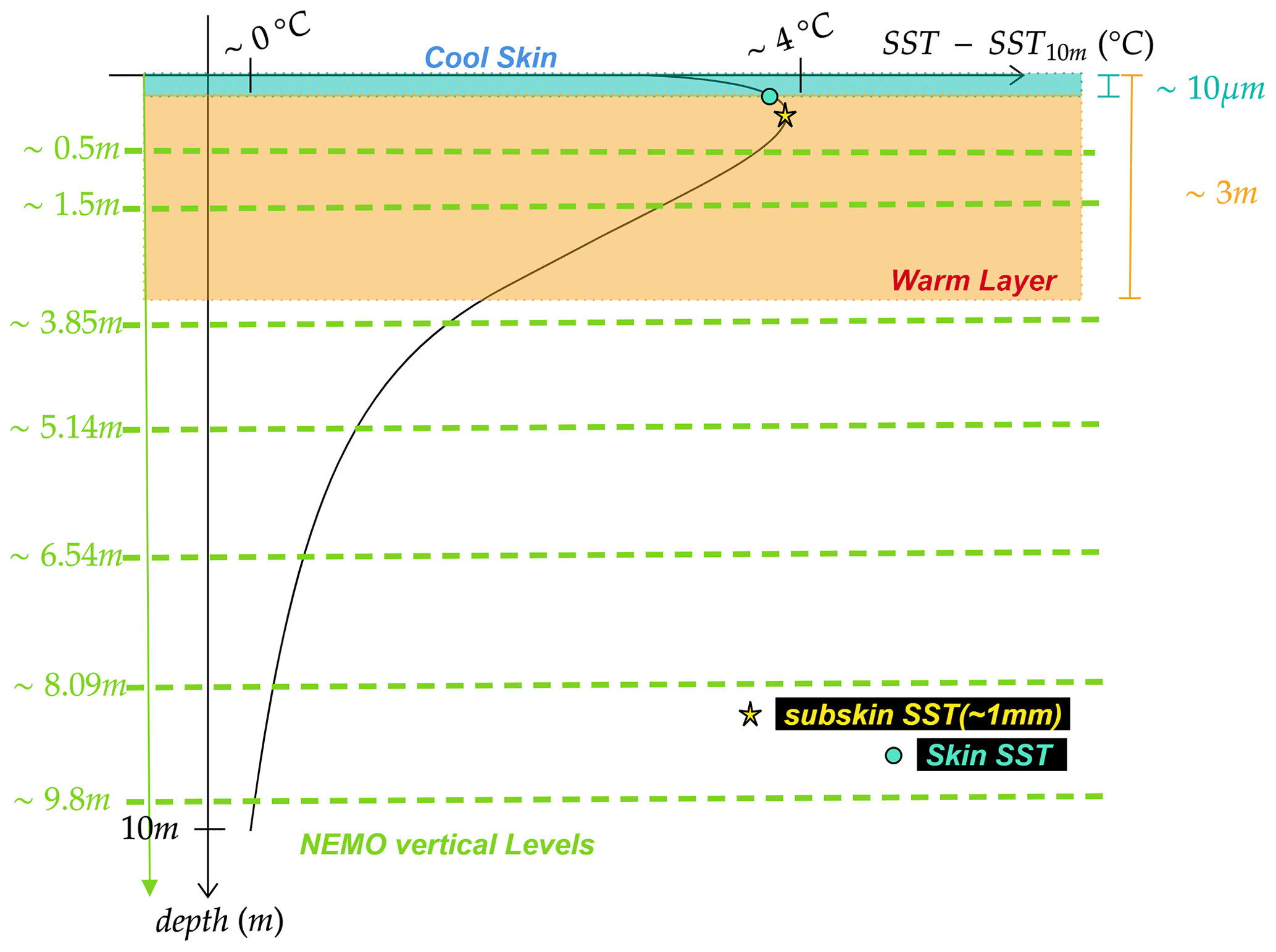
Figure 1 Sketch of the cool skin and warm layer adapted from Donlon et al. (2007). Vertical discretisation of NEMO levels is shown in green (not perfectly in scale with the underlying y axis).

The cool-skin effect is very important for obtaining accurate estimates of the latent and sensible heat flux, especially because its consideration modifies specific humidity at the ocean surface, which is one of the factors in the bulk formula. Indeed, latent and sensible heat fluxes are defined as the heat transfer across the ocean–atmosphere interface due to turbulent air motions (the former including the one resulting from condensation or evaporation). For example, a recent study in the South China Sea showed that during nighttime the cool-skin temperature difference is around 1 K, and there is currently a large uncertainty in the Saunders' constant (Zhang et al., 2021). A warm layer (in which diurnal warming effectively takes place) develops below this cool skin, and its extent reaches a depth at which the penetration of solar radiation can be neglected (usually fixed to 3 m by most existing parameterisations; see Sect. 3.3 for more details). Diurnal warm-layer anomalies (which can sometimes exceed 3 K) can potentially impact both the atmosphere and ocean mean state on a variety of spatial (ranging from regional, basin-wide to global ones) and temporal scales (relevant for weather or seasonal forecast to long-term climatic trends) (Donlon et al., 2007). The skin SST diurnal warming amplitude increases under low surface winds (smaller than 2 m s⁻¹) and intense solar radiation (higher than typical daily peaks, around 900 W m⁻²) conditions, smaller in winter and at the poles than in summer and in the tropics. The accuracy of skin SST models, and therefore their ability to reconstruct skin SST diurnal variations, is crucial, especially in heat budget closure problems, which are still a subject of active debate, especially in climate change hot spot regions such as the Mediterranean domain (see Marullo et al., 2021, and references therein). Skin SST schemes are also crucial for assimilating daytime SST data from satellite sensors (Penny et al., 2019; Storto and Oddo, 2019; Jansen et al., 2019), with obvious impact on the accuracy of numerical weather and ocean predictions; a correct account of skin SST diurnal variations in turn is crucial for flux calculations, which is already a very delicate problem also from an instrumental point of view.

Within these prognostic schemes, seawater's transparency conditions (e.g. estimated using chlorophyll concentration) have great implications in the way solar radiation is absorbed within the ocean's uppermost layer (Morel and Antoine, 1994). Ohlmann et al. (2000) quantified with the help of radiative transfer calculations the effects of physical and biological processes on solar radiation transmission, classifying chlorophyll concentration, cloud cover, and solar zenith angle as the main factors. Ohlmann and Siegel (2000) and Lee et al. (2005) are further examples of how radiative transfer models are used to develop solar transmission parameterisation, which is fit to the sum of exponentials (the number of terms in the sum depending on the variable which has been considered). To the best of our knowledge, these ideas have neither been implemented nor tested within the prognostic scheme for skin SST present in the ocean model NEMO, which just relies on chlorophyll-calibrated coefficients through Gentemann et al. (2009).

Our main aim here is therefore to improve existing skin SST prognostic schemes, investigating the impact of variable seawater's transparency conditions in modelling solar radiation extinction in the upper ocean. The use of chlorophyll concentration as a proxy for seawater's transparency is not new. In fact, given its covariance with Secchi disc depth (estimated from reflectance at various wavelength), it has been often applied by the ocean colour community to study the dynamics of oligotrophic gyres (Leonelli et al., 2022, and references therein). The paper is structured as follows. After this Introduction, we describe the data and coupled modelling system in Sect. 2. The mathematical context in which we developed our new method, whose novelty stands in allowing the warm layer's extent to vary in space and time according to a chlorophyll concentration climatology, follows in Sect. 3. In Sect. 4 we present results, discussing them and drawing conclusions in Sect. 5.

2 Data and modelling system

We describe here the data and the coupled regional modelling system used in this study. Our description here is functional to the scope of this paper and far from a complete depiction of each dataset. We refer readers to the documentation and relevant literature for detailed information on each dataset and model.

2.1 Operational MED DOISST within CMEMS

The MEDiterranean Diurnal Optimally Interpolated Sea Surface Temperature (MED DOISST) product, operationally distributed and freely available within the Copernicus Marine Environmental Service (CMEMS), provides gap-free (L4) hourly mean maps of sub-skin SST at $\mathrm{1}/\mathrm{16}$° horizontal resolution over the Mediterranean domain, covering from 2019 to present. Sub-skin SST is defined as the temperature at the base of the cool-skin layer, typically sensed by microwave radiometers, and representative of a depth of few millimetres from the ocean's surface (Minnet et al., 2019).

This product combines satellite data acquired from the Spinning Enhanced Visible and InfraRed Imager (SEVIRI) and model data from the Mediterranean Forecasting System (MedFS) used as observations and first guess for an optimal interpolation, respectively, giving a L4 field representative of sub-skin SST (see Pisano et al., 2022, and references therein). In all diagnostics involving these data (and presented in the following sections), regions where the percentage of valid SEVIRI measurements is lower than 50 % have been masked out both in CMEMS MED DOISST and our experiments.

2.2 iQuam in situ data

SST from drifter data were used for validation purposes and acquired from the iQuam (In situ SST Quality Monitor) archive (Xu and Ignatov, 2014). The iQuam provides high-quality and quality-controlled (QC) in situ SST data collected from various platforms, such as drifters, Argo Floats, ships, and tropical and coastal moored buoys. The iQuam SST data are also provided along with quality level flags ranging from 0 to 5, with 5 corresponding to the highest quality level (Xu and Ignatov, 2014). For this study, SST with quality level equal to five were selected from drifters only, since they provide the temperature measurement closest to the surface (compared to the other available instruments), ranging between 20–30 cm (depending on the drifter type).

Additionally, we interpolated model outputs on drifters' location in time and space. Table S1 outlines the number of available measurements for each given month and hour of the day. A total number of 555 919 records were available after the quality flag and platform selection, with the month of April being the most populated one, with 222 996 measurements, and 10 361 measurements at 09:00 LT (local time).

2.3 EN4 objective analysis

EN4, the quality-controlled subsurface ocean temperature and salinity profiles and objective analyses, were used to assess the impact on the temperature vertical profiles. To facilitate the comparison, we made use of the objective analyses after bias corrections of expendable bathythermograph (XBT) calibrations (Gouretski and Reseghetti, 2010; Gouretski and Cheng, 2020), which give a gridded version of the dataset on a 1° regular grid. In the comparison, model outputs were interpolated on this grid.

2.4 Mediterranean chlorophyll concentration

Chlorophyll data were used to estimate the seasonality of e-folding depth (see Methods, Sect. 3). These data are a daily interpolation at 0.3 km horizontal resolution over the Mediterranean domain, and result from a merging between multiple sensors (MERIS – MEdium Resolution Imaging Spectrometer from ESA, SeaWiFS – Sea-viewing Wide Field-of-view Sensor and MODIS – Moderate Resolution Imaging Spectroradiometer from NASA, VIIRS – Visible Infrared Imager Radiometer Suite from NOAA, and most recently the Copernicus Sentinel 3A OLCI – Ocean and Land Colour Instrument), as detailed in the product description (see Volpe et al., 2019, and references therein for further details).

2.5 ECMWF Atmospheric Reanalysis – ERA5

We used heat fluxes (net solar radiation, latent and sensible heat fluxes, net thermal radiation) from ERA5 at 0.25° horizontal and hourly temporal resolution (Hersbach et al., 2020) as reference for comparing performances across simulations with different skin SST schemes. Despite their possible biases in air–sea fluxes, atmospheric reanalyses today are still widely thought to provide the best gap-free and dynamically consistent reconstructions of the atmosphere system (Valdivieso et al., 2017; Storto et al., 2019).

2.6 Mixed-layer depth 1969–2013 climatology

Data from a mixed-layer depth (MLD) climatology was used to test to what extent our modified scheme correctly represents the seasonality of the mixed layer.

This monthly gridded climatology was produced using mechanical bathythermograph (MBT), expendable bathythermograph (XBT), profiling floats, gliders, and ship-based CTD (conductivity, temperature, depth) data from different databases and carried out in the Mediterranean Sea between 1969 and 2013. As for the model outputs, MLD is calculated with a ΔT=0.1 °C criterion relative to 10 m reference level on individual profiles (Houpert et al., 2015a, b).

2.7 ISMAR Mediterranean Earth System Model (MESMAR)

MESMAR is a newly developed coupled regional modelling framework for the Mediterranean region (Storto et al., 2023a). MESMAR includes the following components.

• the ocean model NEMO v4.0.7, with horizontal resolution of about 7 km, 72 unevenly spaced vertical levels (the first and the last levels being, respectively, about 0.5 and 200 m thick) and a time step of 7.5 min (NEMO System Team, 2019);

• the atmosphere model WRF v4.3.3, with 41 vertical hybrid levels and horizontal resolution of about 15 km, covering the European branch of the international Coordinated Downscaling Experiment (EURO-CORDEX) domain, and a time step of 1 min (Skamarock et al., 2021);

• the interactive runoff model HD v5.0.1, with a time step of 30 min and $\mathrm{1}/\mathrm{12}$° horizontal resolution over Europe (Hagemann et al., 2020);

• the coupler OASIS3-MCT, coupling the three models with a coupling frequency of 30 min and using the SCRIP library to interpolate fields between different model grids (Craig et al., 2017);

We report in Fig. 2 a graphical summary of different grids. Further details of its implementation, tuning, and performance are described in (Storto et al., 2023a).

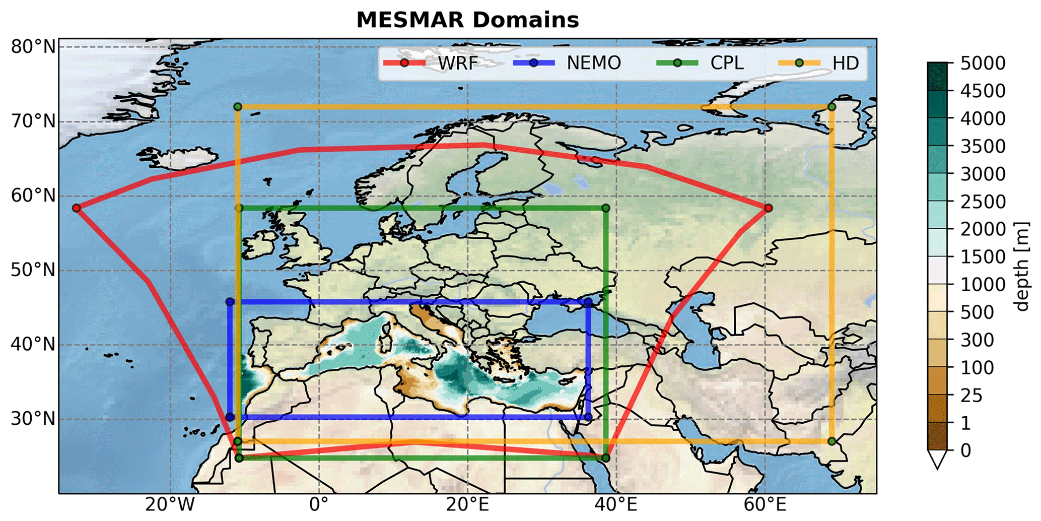
Figure 2 The modelling system domain. WRF, NEMO, HD, and boundaries for the coupling mask are shown in red, blue, orange, and green, respectively. The contour-filled plot shows the ocean model bathymetry.

3 Methods

Many schemes to reconstruct the skin SST diurnal variations rely on the existence of a cool skin and a warm layer in the upper micrometres and few metres of the ocean, respectively, whose dynamics strongly depends on wind conditions and solar radiation extinction within the upper ocean. To explain the rationale behind the developments in our new method, we need to recap here some elements of this theory, which is mostly based on Zeng and Beljaars (2005) (named ZB05, hereafter) work.

We start from the one-dimensional heat transfer equation in the ocean:

$$\begin{array}{}\text{(1)}& {\displaystyle \frac{\partial T}{\partial t}}={\displaystyle \frac{\partial }{\partial z}}\left(K_{\mathrm{w}}+k_{\mathrm{w}}\right){\displaystyle \frac{\partial T}{\partial z}}+{\displaystyle \frac{\mathrm{1}}{{\mathit{\rho }}_{\mathrm{w}}{c}_{\mathrm{w}}}}{\displaystyle \frac{\partial R}{\partial z}},\end{array}$$

in which the subscript w refers to water properties; T is seawater temperature (K), K_w (m² s⁻¹) is the turbulent diffusion coefficient; k_w (m² s⁻¹) is the molecular thermal conductivity; ρ_w (kg m⁻³) and c_w (J Kg⁻¹ K⁻¹) are, respectively, seawater density and heat capacity per unit volume; R (W m⁻²) is the net solar radiation flux, defined as positive downward.

3.1 Cool skin

We assume that there is an oceanic molecular sublayer of depth δ, where K_w is negligible and temperature can be assumed constant in time since it is always cooler than the temperature of the underlying seawater (Donlon et al., 2007; Zeng and Beljaars, 2005). Thus, integration of Eq. (1) gives the following equation, $\forall z\in [\mathrm{0},-\mathit{\delta }]$,

$$\begin{array}{}\text{(2)}& k_{\mathrm{w}}{\displaystyle \frac{\partial T}{\partial z}}+{\displaystyle \frac{\mathrm{1}}{{\mathit{\rho }}_{\mathrm{w}}{c}_{\mathrm{w}}}}\left[R\left(z\right)-R_{\mathrm{s}}\right]-\textcolor{red}{}=\text{const},\end{array}$$

where R_s is the net solar radiation at the surface (constant, open-ocean albedo, since the Mediterranean Sea is an ice-free basin) and the last term at the left-hand side is negligible up to order z². Assuming this constant to be the top boundary condition at z=0:

$$\begin{array}{}\text{(3)}& {\mathit{\rho }}_{\mathrm{w}}{c}_{\mathrm{w}}{k}_{\mathrm{w}}{\displaystyle \frac{\partial T}{\partial z}}{}_{z=\mathrm{0}}=Q=\text{LH}+\text{SH}+\text{LW},\end{array}$$

in which LH, SH, and LW are, respectively, the surface fluxes of latent heat, sensible heat, and net long-wave radiation.

Thus, Eq. (2) can be rewritten as

$$\begin{array}{}\text{(4)}& {\mathit{\rho }}_{\mathrm{w}}{c}_{\mathrm{w}}{k}_{\mathrm{w}}{\displaystyle \frac{\partial T}{\partial z}}=Q+R_{\mathrm{s}}-R\left(z\right).\end{array}$$

Making a further integration we get the following cool-skin temperature difference:

$$\begin{array}{}\text{(5)}& T_{\mathrm{s}}-T_{-\mathit{\delta }}={\displaystyle \frac{\mathit{\delta }}{{\mathit{\rho }}_{\mathrm{w}}{c}_{\mathrm{w}}{k}_{\mathrm{w}}}}\left(Q+f_{\mathrm{s}}{R}_{\mathrm{s}}\right),\end{array}$$

where T_s and T_−δ are, respectively, the temperature at the upper (air–sea interface) and lower limits of the cool-skin layer, while f_s is the fraction of solar radiation absorbed in this layer:

$$\begin{array}{}\text{(6)}& f_{\mathrm{s}}={\displaystyle \frac{\mathrm{1}}{\mathit{\delta }}}\underset{-\mathit{\delta }}{\overset{\mathrm{0}}{\int }}\left(\mathrm{1}-{\displaystyle \frac{R\left(z\right)}{R_{\mathrm{s}}}}\right)\mathrm{d}z,\end{array}$$

which depends on the way radiation gets absorbed within the cool skin. Being time-independent, the cool-skin temperature difference is a diagnostic variable in the scheme.

Equation (5) is analogous to Saunders' model. Indeed, Saunders (1967) was one of the first to construct a theory for the ocean “cool-skin” effect, i.e. the observed temperature at the air–sea interface is generally cooler than the temperature of the water at about 10 cm depth, especially during nighttime. This effect takes place mainly because of the transfer of energy between the ocean and the atmosphere, realised via heat loss and momentum transfers (wind stress). In a nutshell, at the end of its derivation (Saunders, 1967), he obtains the following expression for the temperature difference across the cool skin, ΔT_c (K):

$$\begin{array}{}\text{(7)}& \mathrm{\Delta }{T}_{\mathrm{c}}=\mathit{\lambda }{\displaystyle \frac{Q{\mathit{\nu }}_{\mathrm{w}}}{k_{\mathrm{w}}(\mathit{\tau }/{\mathit{\rho }}_{\mathrm{w}}{)}^{\mathrm{1}/\mathrm{2}}}},\end{array}$$

where λ is the Saunders' proportionality constant; Q (W m⁻²) has already been defined above; $\mathit{\tau }/{\mathit{\rho }}_{\mathrm{w}}$ (m² s⁻²) is the kinematic stress (ratio between wind stress module and seawater density); and ν_w (m² s⁻¹) and k_w (m² s⁻¹) are the kinematic viscosity and thermal conductivity of seawater, respectively. Saunders' formulation was originally conceived for low, nonzero wind conditions and neglected the effect of solar radiation (it recognised its role and added a discussion on how to account for it in the model only at the end of the paper). As noticed by Fairall et al. (1996) and Artale et al. (2002) (named A02 hereafter), with a constant λ Eq. (6) becomes problematic in limiting cases of low and very high wind speeds (greater than 7 m s⁻¹) because the wind stress in the denominator limits its validity. Thus, A02 proposed to include a wind dependence in Saunders' constant in order to still have a finite, nonzero cool skin to bulk temperature difference even when the wind speed goes to zero or becomes very high. This scheme has proven to have good performances compared to other schemes also on a mooring site in the Pacific Ocean (Tu and Tsuang, 2005).

3.2 Warm layer

Below the skin layer, turbulent transfer is much more effective, and k_wcan be neglected in favour of K_w. Integrating Eq. (1) within the $[-d,-\mathit{\delta }]$ layer, we get

$$\begin{array}{}\text{(8)}& {\displaystyle \frac{\partial }{\partial t}}\underset{-d}{\overset{-\mathit{\delta }}{\int }}T\mathrm{d}z={\displaystyle \frac{Q+R_{\mathrm{s}}-R\left(-d\right)}{{\mathit{\rho }}_{\mathrm{w}}{c}_{\mathrm{w}}}}-K_{\mathrm{w}}{\displaystyle \frac{\partial T}{\partial z}}{}_{z=-d},\end{array}$$

where d is a reference depth that can be assumed as the depth at which the diurnal cycle can be omitted.

The turbulent diffusion coefficient can be expressed as follows (Large et al., 1994):

$$\begin{array}{}\text{(9)}& K_{\mathrm{w}}=k{u}_{\ast \mathrm{w}}\left(-z\right)/{\mathit{\varphi }}_t\left({\displaystyle \frac{-z}{L}}\right),\end{array}$$

in which k=0.4 is the Von Kármán constant, z is negative in the ocean, and u_∗w is the friction velocity in the water (this being the air friction velocity multiplied by the square root of air-to-sea density ratio). The stability function ϕ_t discriminates between a stable and an unstable regime, depending on the sign of its argument, which is the ratio of the vertical coordinate to the Monin–Obukhov length L: positive for the stable one and negative for the unstable one. Assuming z to be negative in the ocean, the change in sign entirely depends on the Monin–Obukhov length, which is a length characterising the prevalence of buoyancy-variation-induced turbulence over the one generated by wind shear effects. This in turn is strongly dependent on the sign of the net heat flux Q. If Q>0, i.e. the ocean gains heat from the atmosphere, and we have the stable regime, the diffusion coefficients decrease with increasing depth, favouring the downward heat transfer within the water column. The opposite case, which favours transfer of heat from the ocean to the atmosphere, can be modelled in different ways (see While et al., 2017, and references therein).

Assuming a temperature dependence, for d≫δ of the form

$$\begin{array}{}\text{(10)}& T=T_{-\mathit{\delta }}-{\left[{\displaystyle \frac{z+\mathit{\delta }}{-d+\mathit{\delta }}}\right]}^{\mathit{\nu }}\left(T_{-\mathit{\delta }}-T_{-d}\right)\mathit{\nu }\text{ empirical parameter},\end{array}$$

Eq. (7) simplifies to

$$\begin{array}{}\text{(11)}& \begin{array}{rl}{\displaystyle \frac{\partial }{\partial t}}\left(T_{-\mathit{\delta }}-T_{-d}\right)& ={\displaystyle \frac{Q+R_{\mathrm{s}}-R\left(-d\right)}{d{\mathit{\rho }}_{\mathrm{w}}{c}_{\mathrm{w}}}}{\displaystyle \frac{\mathit{\nu }+\mathrm{1}}{\mathit{\nu }}}\\ & -{\displaystyle \frac{\left(\mathit{\nu }+\mathrm{1}\right)k{u}_{\ast w}}{d{\mathit{\varphi }}_t\left(d/L\right)}}\left(T_{-\mathit{\delta }}-T_{-d}\right)\end{array},\end{array}$$

In the ZB05 scheme (Zeng and Beljaars, 2005), Eqs. (5) and (10) are the coupled equations for the cool skin (diagnostic part) and warm layer (prognostic part), respectively. Being time dependent, the determination of the warm-layer temperature difference at time t requires the knowledge of the one at the previous time step, and thus is the prognostic variable in the scheme. Assumptions on the fraction of solar radiation within the warm layer and the cool-skin depth usually follow Fairall et al. (1996) parameterisation, the details of which are given in the Supplement.

3.3 Solar transmission expression

The expression of the solar transmission in Zeng and Beljaars (2005) is

$$\begin{array}{}\text{(12)}& {\displaystyle \frac{R\left(-d\right)}{R_{\mathrm{s}}}}=\sum _{i=\mathrm{1}}^{\mathrm{3}}{a}_i{e}^{-d{b}_i}\text{ where}\begin{array}{l}\left(a_{\mathrm{1}},a_{\mathrm{2}},a_{\mathrm{3}}\right)=\left(\mathrm{0.28},\mathrm{0.27},\mathrm{0.45}\right),\\ \left(b_{\mathrm{1}},b_{\mathrm{2}},b_{\mathrm{3}}\right)=\left(\mathrm{71.5},\mathrm{2.8},\mathrm{0.07}\right)m^{-\mathrm{1}}\end{array},\end{array}$$

following Soloviev formulation (Soloviev, 1982) (S82 in the following), which is very widely used in atmosphere models (such as WRF, Skamarock et al., 2021).

So far this is not the only possibility: a formulation with 61 coefficients has been developed by Jerlov (1968), which is based on different water types classified based on chlorophyll concentration and particulates, for light in the visible spectrum.

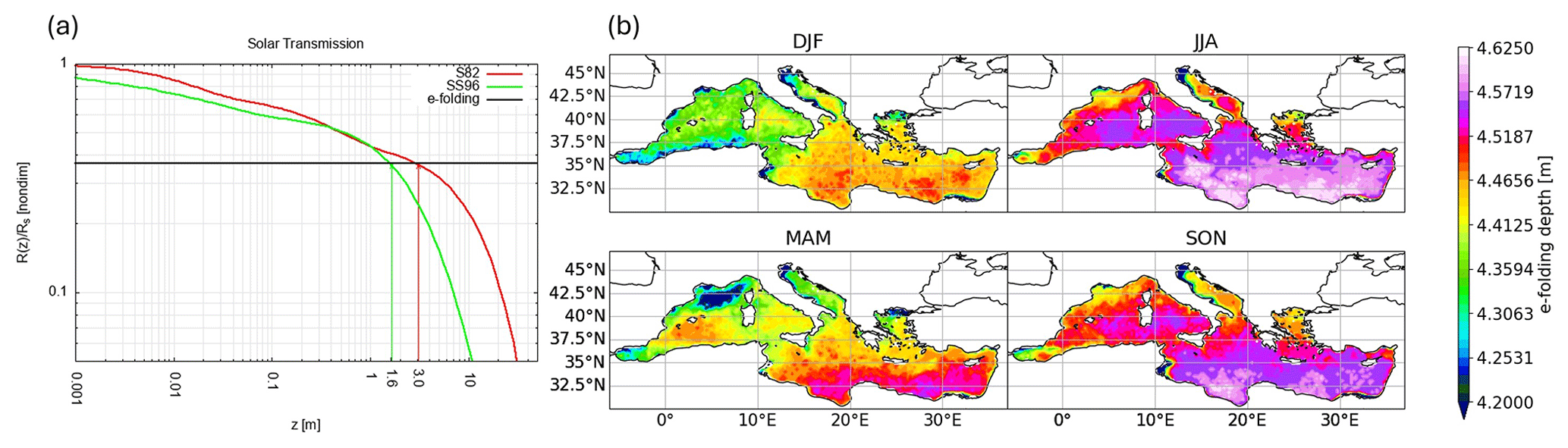
Figure 3 Panel (a) shows two different formulations frequently used for the transmission coefficient expression: the red curve shows the formulation of Soloviev (1982), while the green curve shows the one defined in Soloviev and Schlussel (1996). Panel (b) shows e-folding-depth estimates from Mediterranean chlorophyll climatology of Volpe et al. (2019): the lowest values touch the 2.5 m depth. Note that the x-axis range does not start from 0 to allow a logarithmic representation of the depth.

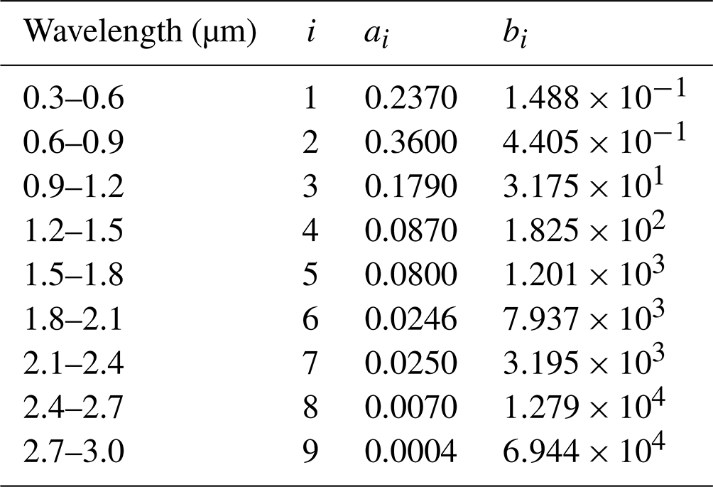
Formulations with nine coefficients (reported in Table 2) have been proposed to include such effects: for example, Soloviev and Schlussel (1996) use a different coefficient for the first term depending on Jerlov's optical water type, while Gentemann et al. (2009) include solar angle in the parameterisation, keeping the value of the first coefficient as in the case of pure water. Without knowing what the Jerlov water type is, what is currently implemented in NEMO is to take b₁ as the average between coefficients for the I, IA, IB, II, and III Jerlov optical water types. This formulation is widely employed in ocean models (such as in the optional skin SST routine of NEMO; see While et al., 2017), with the reference depth d fixed to 3 m. Therefore, the solar transmission is as follows:

$$\begin{array}{}\text{(13)}& {\displaystyle \frac{R\left(-d\right)}{R_{\mathrm{s}}}}=\sum _{i=\mathrm{1}}^{\mathrm{9}}{a}_i{e}^{-d{b}_i}.\end{array}$$

Ideally, one would like to have a reference depth representative of the one at which the transmission of solar radiation is negligible, and if we take it as the depth at which transmission drops to $\mathrm{1}/e$ from its surface value, we get a value that can be different from d=3 m, as we can see from Fig. 3a. Allowing for a realistic time- and space-varying value of d represents the main novelty of our work.

From this viewpoint, choosing a value of d=3 m while using the solar extinction formulation as in Soloviev (1982) or Soloviev and Schlussel (1996) would lead to underestimating the penetration of solar radiation into the warm layer. Another possibility, which constitutes our modification to the scheme already implemented in NEMO, is to reconstruct a chlorophyll profile from its surface values following what is already implemented in the NEMO module for radiation calculations (Jerlov, 1968; Morel and Berthon, 1989; Lengaigne et al., 2007) and employ an RGB + Chl a scheme to calculate radiation as a function of depth. Then, from Eq. (13) with only four terms (one for chlorophyll, and three for RGB, expressed in lookup tables), one can numerically derive the warm-layer reference depth as the e-folding depth of the light extinction profile (see Fortran source files in the Zenodo repository; de Toma, 2024).

This would give a constant transmission throughout the basin but with a spatially and temporally varying e-folding depth and defines our new prognostic scheme for skin SST warm-layer calculation, thus embedding in it the ocean colour information coming from Chl a. Everything else is left unchanged, both the refinements of Takaya et al. (2010), which include the effect of Langmuir circulation and a modification of the Monin–Obukhov similarity function under stable conditions (T10 hereafter), and the A02 model for cool skin, which has been demonstrated to improve the scheme under wavy and windy conditions, respectively.

The e-folding depth estimates

Mediterranean chlorophyll climatology data (see Sect. 2.4) were re-gridded onto a 0.25° regular longitude–latitude grid, and tabulated coefficients within NEMO were used to retrieve the transmission, accounting for chlorophyll variations. The r-folding depths can then be estimated as the depth at which transmission drops to $\mathrm{1}/e$ from its surface value. It can be noticed from Fig. 3b that the e-folding depth also varies with seasonality, with typical values ranging from about 3 to 4.5 m. This is the central point of our modification to the prognostic scheme. In our setup we extracted the e-folding depth used within the prognostic scheme pixel-wise and at each time step of the NEMO model.

Table 1 Overview of the simulations performed.

Table 2 Parameters for the transmission coefficient following Soloviev and Schlussel (1996), in which the first coefficient is the average between the one corresponding to the I, IA, IB, II, and III Jerlov optical water types. This is currently implemented in NEMO.

3.4 Overview of the simulations performed

With the coupled ocean–atmosphere regional system we performed a set of four simulations forced by ERA5 in the atmosphere and ORAS5 (Zuo et al., 2018) in the ocean and covering 3 years (from 2019 to 2021) with hourly outputs (a synthesis is provided in Table 1). In cases where a skin SST scheme is active, we substitute the SST, i.e. temperature on the first NEMO level, with the skin SST coming out from the scheme.

1. The first simulation is a control run in which no skin SST prognostic scheme is activated; therefore, the diurnal SST variations in the uppermost ocean layer (0.5 m thick) only come from the variability represented by the ocean model at about 0.5 m depth and also consider the 0.5 h frequency of the coupling. We will refer to this experiment in the following as ctrlnoskin.

2. The second simulation is a run in which the ZB05 scheme in WRF (Zeng and Beljaars, 2005) is active. We shall refer to this case in the following aswrfskin.

3. The third simulation is a run in which the existing scheme within NEMO is used that employs the nine-coefficient parameterisation for light extinction coefficients (Gentemann et al., 2009 – G09 hereafter), the scheme for the cool skin as modified in A02, and refinements of the stability function in the warm-layer formulation as in T10. We shall refer to this as the nemoskwrite case.

4. The fourth simulation is a run where we modified the reference depth for the basis of the warm layer from z=3 m to an e-folding depth (i.e. the depth at which radiation gets diminished by $\mathrm{1}/e$ from its surface value) that is allowed to vary temporally and spatially because it is estimated from RGB light extinction coefficients and chlorophyll concentration (see Sect. 3). We will refer to it as modradnemo, and it is the experiment where our modification to the skin SST scheme is implemented and tested.

The reason behind the choice of the above-mentioned period of 3 years (2019–2021) is twofold: first, it allows a validation against all the measurements from different data sources (satellite, drifters, and objectively analysed profiles), and, second, it is a good trade-off between the needs of keeping a reasonable computational load and data volume for the analysis and guarantees a minimal robustness of our finding compared to a simulation that covers just 1 year. However, we do not discard the possibility of extending the time coverage in our plans for future works.

4 Results

In this section, we present skill scores against satellite, drifter, and temperature profile data (see Sect. 2) from the set of the simulations performed, aimed at characterising the impacts of our modified skin SST scheme. Since we are mainly acting to improve skin SST diurnal variation reconstruction in the ocean component, the main focus is on the difference between the nemoskwrite and modradnemo, while the ctrlnoskin and wrfskin ones are included as further reference elements (the latter being not directly comparable because the atmospheric model sees the ocean foundation SST and employs the scheme just to diagnose the skinSST).

4.1 Comparison with CMEMS MED DOISST

We calculated the mean diurnal warming amplitude in each season as the seasonally averaged diurnal warming amplitudes (diurnal warming amplitude being defined for each day as the difference between daytime maximum and nighttime minimum of SST), which can be cast into the following equation:

$$\begin{array}{}\text{(14)}& \begin{array}{rl}{〈\mathrm{DWA}〉}_{\mathrm{seas}}& ={\displaystyle \frac{\mathrm{1}}{N_{\mathrm{seas}}}}{\sum }_{i=\mathrm{1}}^{N_{\mathrm{seas}}}\left\{\begin{array}{c}\text{max}\\ h_i\in [\mathrm{10}:\mathrm{00},\mathrm{18}:\mathrm{00}]\end{array}\mathrm{SST}\left(h_i\right)\right.\\ & \left.-\begin{array}{c}\text{min}\\ h_i\in [\mathrm{00}:\mathrm{00},\mathrm{06}:\mathrm{00}]\end{array}\mathrm{SST}\left(h_i\right)\right\},\end{array}\end{array}$$

where seas (DJF, JJA, MAM, SON) is the given season, N_seas is the number of days in that particular season, and h_i is the local time in hours for any given day.

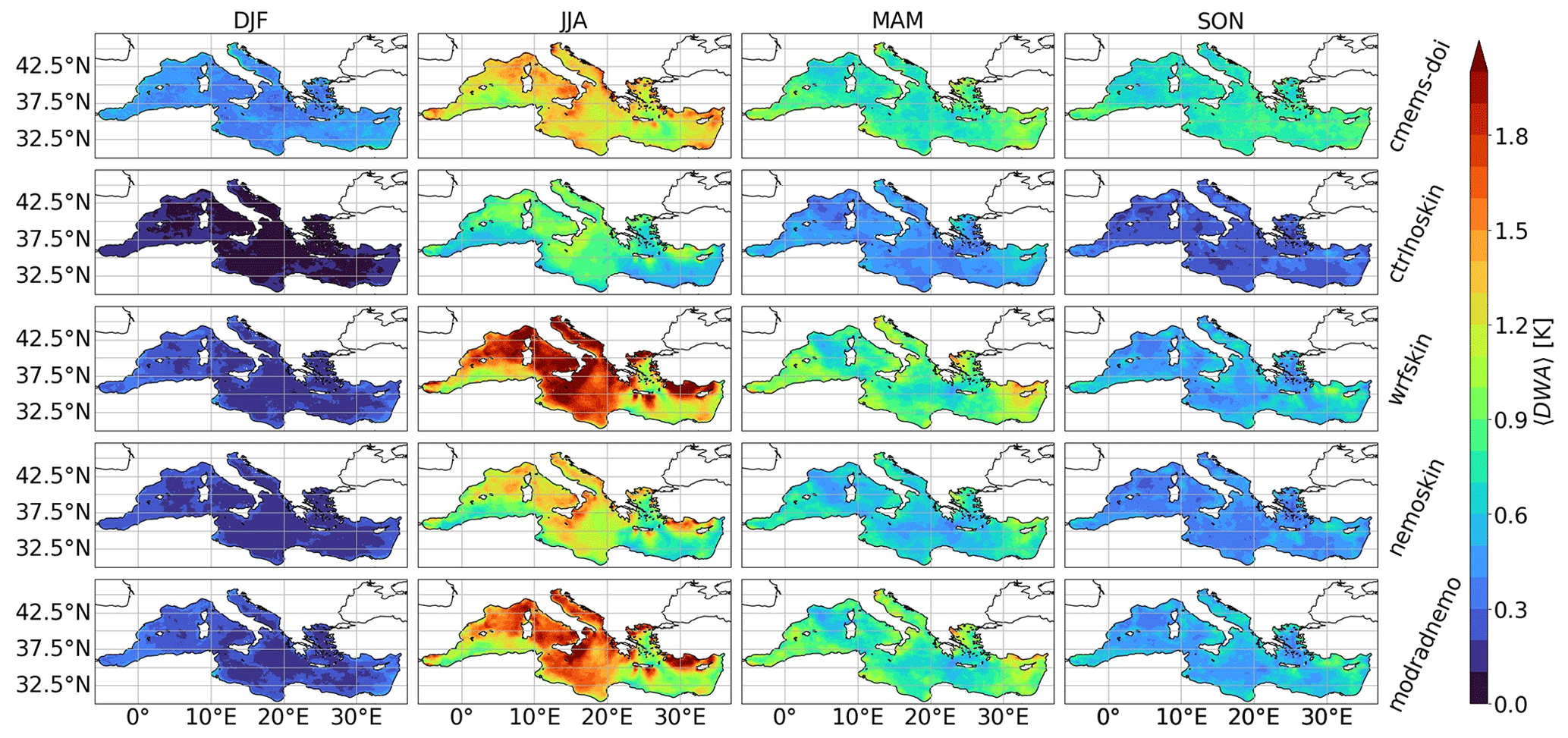
Figure 4 Mean diurnal warming amplitude averaged over each season (columns), for each case (row): the first row is the CMEMS MED DOISST data, followed in order by the control simulation, wrfskin, nemoskwrite, and modradnemo.

Seasonally averaged diurnal warming amplitudes are shown in Fig. 4. On average, the maximum amplitude is reached in summer, with the wrfskin simulation peaking at about 3 K, thus overestimating the mean diurnal cycle compared to CMEMS MED DOISST (the monthly biases with respect to CMEMS foundation SST both in the western and the eastern part of the Mediterranean Sea stay below 1 K year-round for all of the simulations performed – see Fig. S1 in the Supplement). The nemoskwrite simulation yields a pattern very similar to CMEMS MED DOISST in summer but underestimates the signal in the remaining seasons. Outside the summer season, our modifications yield a slight improvement (see modradnemo, last row of Fig. 4). As expected, the control run in which no skin SST method is active generally underestimates the diurnal signal everywhere. Compared to nemoskwrite, the modradnemo simulation improves JJA mean diurnal warming amplitude, especially over the southern Mediterranean Sea, while in central and northern part of the basin it tends to overestimate the signal by about 0.5 K with respect to CMEMS-DOI data. Furthermore, a general underestimation is present also in DJF, with the modradnemo simulation showing the smallest differences with respect to CMEMS-DOI data.

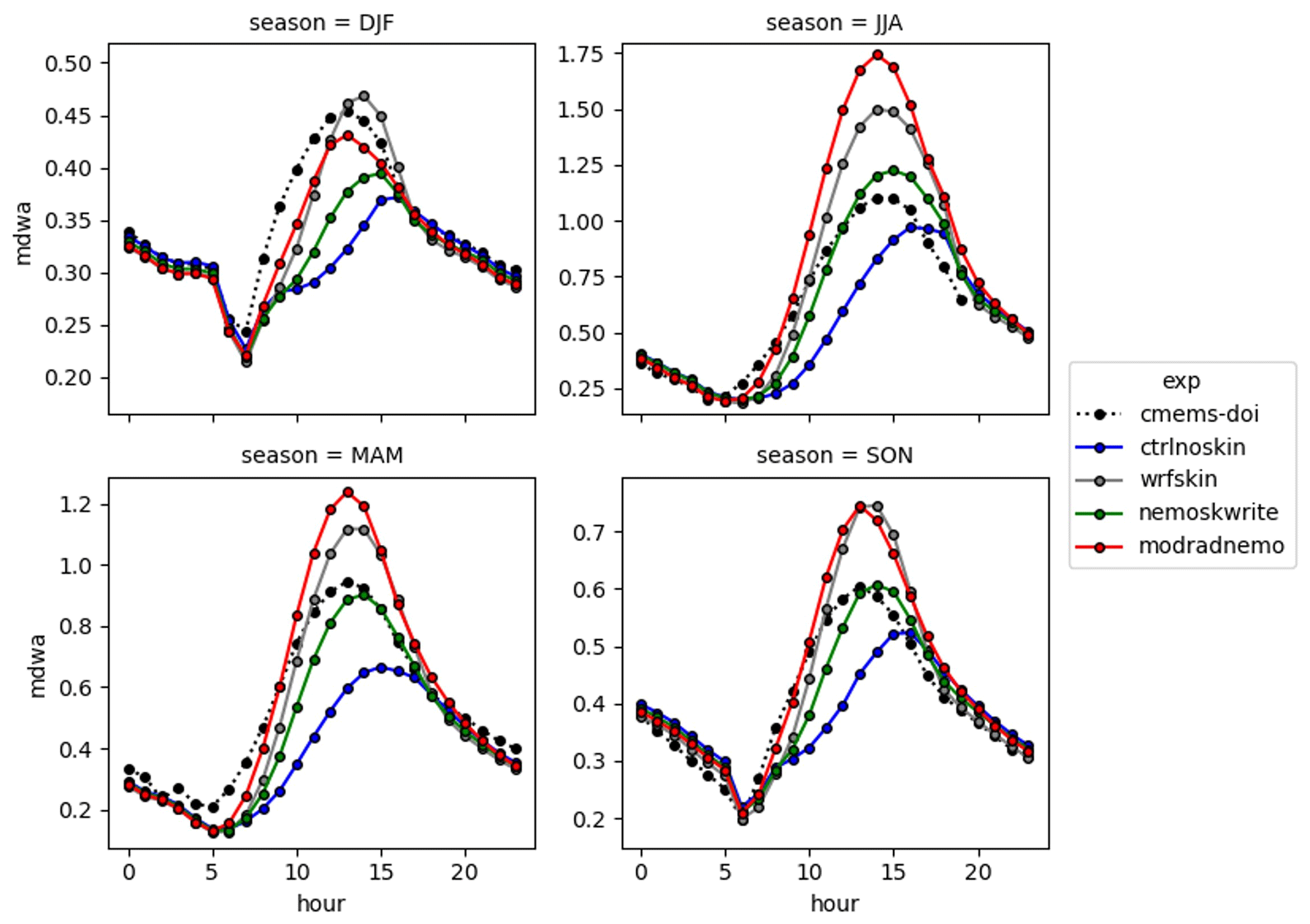
Figure 5 Seasonality of the diurnal cycle averaged over the whole Mediterranean Sea, masking out regions in time and space where the percentage of model data in CMEMSDOI is greater than 50 %.

The spatial average over the whole Mediterranean domain is shown in Fig. 5, confirming the general underestimation of the control run and the overestimation of the wrfskin and modradnemo in all seasons except winter.

Computing spatial averages highlights that modradnemo slightly improves the mean diurnal warming amplitude signal during wintertime, while in all the other seasons the best agreement is gained using the nemoskwrite setup (ZB05 with T10 and A02 modifications), at least according to the verification against CMEMS MED DOISST.

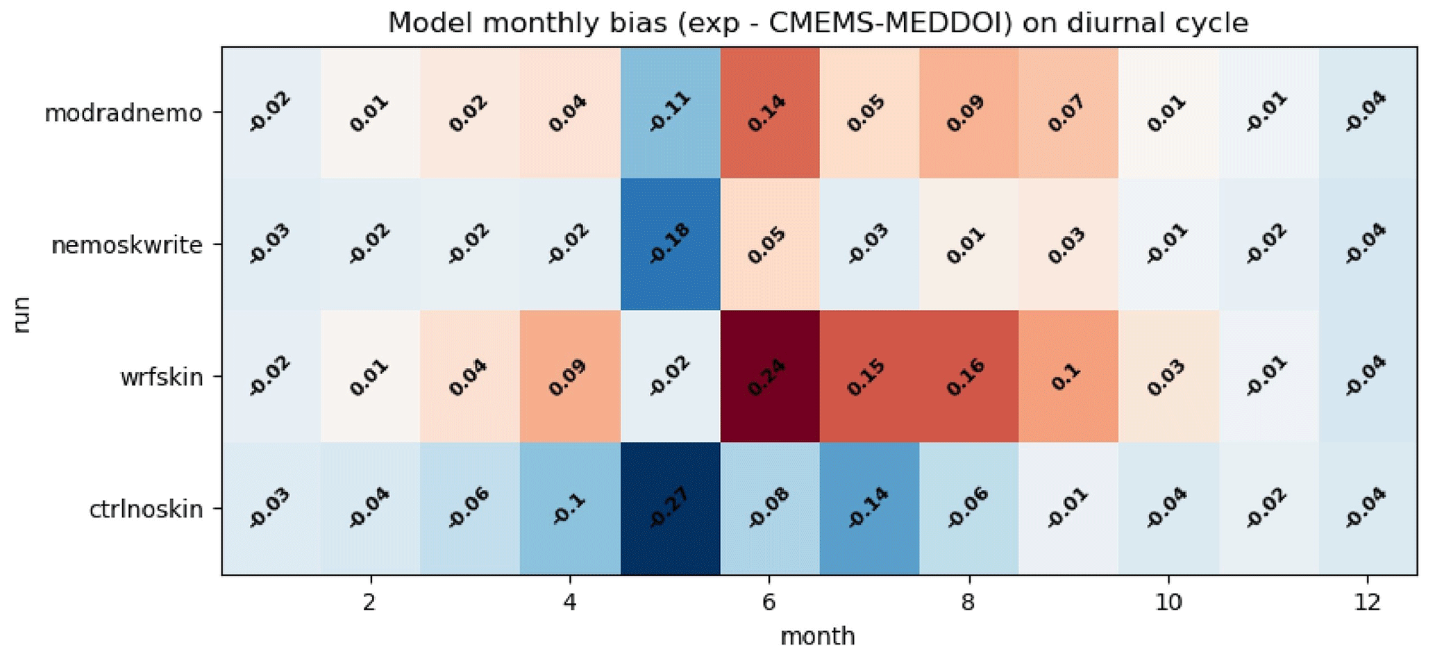
Figure 6 Monthly averaged values for the time series of spatial mean diurnal cycle over the Mediterranean Sea (bias with respect to CMEMS MED DOISST).

On a monthly timescale, Fig. 6 confirms that the control simulation generally tends to have a negative bias in the diurnal amplitude for the whole simulated period. The wrfskin (ZB05 scheme) shows a warm bias during summertime months, shown just as a reference. The comparison between nemoskwrite (ZB05 + A02 + T10) and modradnemo (Chl–e-folding depth) shows the improvement of our scheme (modradnemo) over the old one (nemoskwrite), especially in May, but not in April, June, July, August, and September, despite the amplitude of the bias being slightly reduced in the rest of the period.

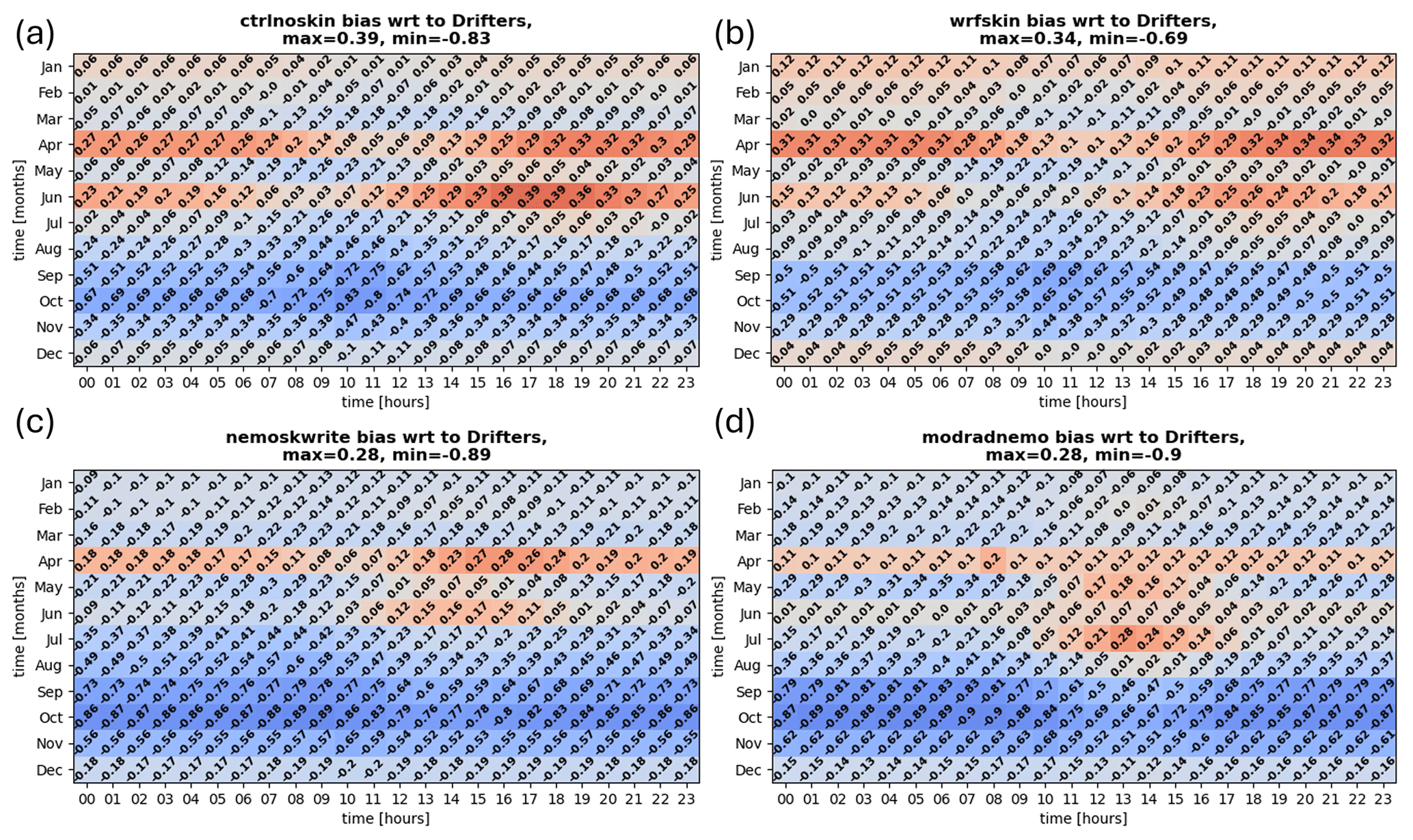
Figure 7 Bias with respect to measurements averaged over drifters' locations as a function of the month and the time of the day. Panels (a), (b), (c), and (d) show, respectively, the results for all the simulations carried out in the present study. Confidence in these numbers can be supported by the numbers of measurements reported in Table S1.

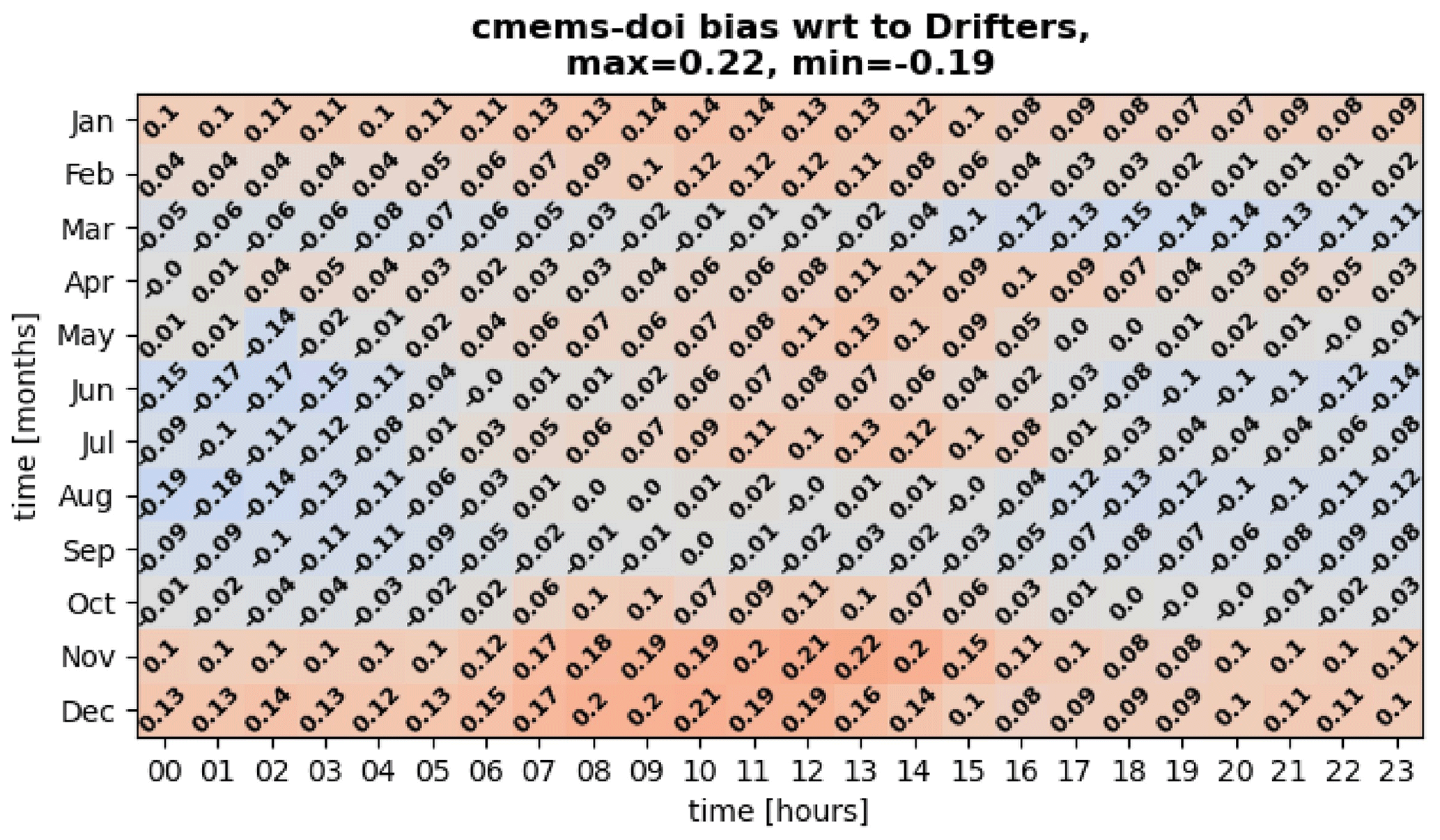
Figure 8 Bias with respect to measurements averaged over drifters' locations as a function of the month and time of the day for CMEMS MED DOISST data.

4.2 Comparison with iQuam Star high-resolution (HR) drifters

The bias with respect to drifter measurements averaged over drifters positions as a function of the month and time of the day is shown in Fig. 7. All the schemes present a systematic cool bias in autumn (SON) for most of the hours of the day. During April and June, the modradnemo simulation significantly reduced the warm bias with respect to observations compared to the nemoskwrite case, keeping it generally positive. This is quite reasonable, since drifter measurements can be thought of as representative of a depth that can also be below the sub-skin level (typically on the order of some centimetres). Consistently with Fig. 6, the wrfskin has a larger positive bias than modradnemo in June.

Further, as shown by Fig. 8, the bias between CMEMS MED DOISST and drifters is generally positive anytime except in late spring–summer and autumn during nighttime. This pattern arises because of the composite effect of having a temperature representative of the sub-skin level where and when there are data from radiometers, and a temperature of about 1 m depth from the MEDFS (MEDiterranean Forecasting System) as a first guess of the optimal interpolation over cloudy regions (Pisano et al., 2022). However, the modified scheme significantly reduces the difference, yielding a bias closer to the one of CMEMS MED DOISST with respect to drifters, especially during April, which is the month in which the number of observations from drifters is definitely larger.

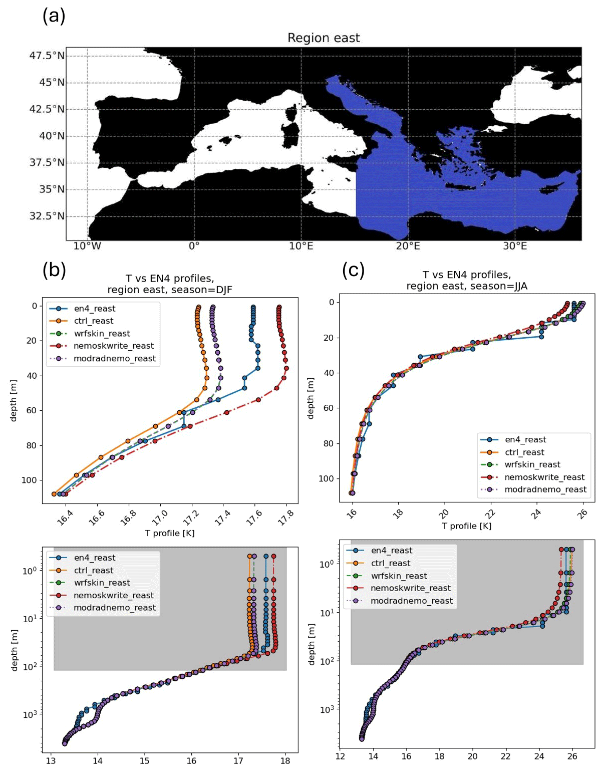
Figure 9 Spatial average of profiles within the eastern Mediterranean Sea during winter and summer. Panel (a) shows the eastern region, while (b) and (c) show, respectively, wintertime and summertime spatially averaged profiles within the top 100 m in the upper part, while on the bottom the whole depth range on a logarithmic scale is shown.

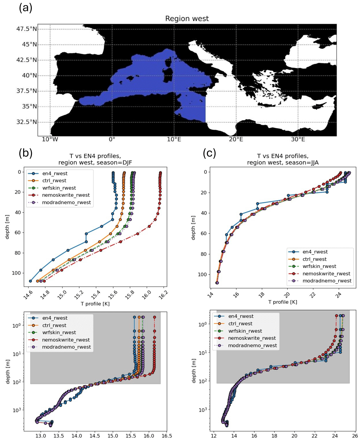
Figure 10 Spatial average of profiles within the eastern Mediterranean Sea, during winter and summer. Panel (a) shows the eastern region, while (b) and (c) show, respectively, wintertime and summertime spatially averaged profiles within the top 100 m in the upper part, while on the bottom the whole depth range on a logarithmic scale is shown.

4.3 Comparison with EN4 objective analysis

Bias-corrected vertical profiles gathered in an objective analysis were used to assess differences across schemes along the water column. To summarise, we report here only a macro subdivision of the eastern and the western Mediterranean Sea, respectively, in Figs. 9 and 10. Model outputs were remapped on the same vertical and horizontal grid. Looking at the mean profile averaged over all grid points in the given area, the agreement is better for all simulations during summertime months, both for the eastern and the western region (see Figs. 9c, 10c), showing in particular that the modradnemo simulation outperforms the nemoskwrite one. This is also true for the wintertime season in the eastern Mediterranean (see Fig. 9b). On the other hand, in the western Mediterranean all simulations tend to overestimate the signal, with our modified scheme doing a better job with respect to the nemoskwrite case, with an average profile that is about 0.4 °C closer to the EN4 profile. However, below about 80 m depth differences across schemes vanish.

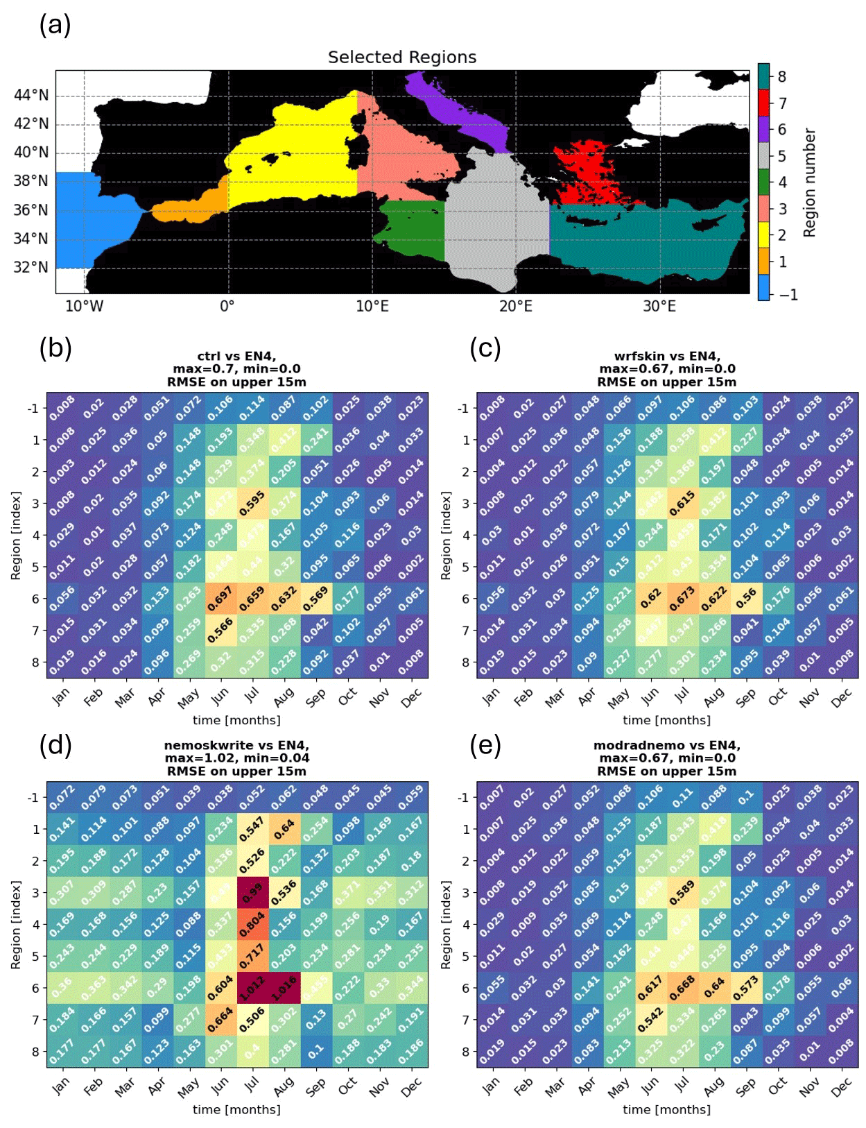
Figure 11 RMSE on the top 15 m of the difference between regionally averaged profiles between each simulation and EN4, displayed as a function of the region and the particular month. Division in regions is reported in panel (a), while (b), (c), (d), and (e) show, respectively, the results for all the simulations carried out in the present study.

Looking in more detail at the RMSE on the top 15 m depth between each simulation and EN4 as a function of the month and more detailed region subdomains shown in Fig. 11a, we can see how in general all simulations present the same pattern for the region outside the Strait of Gibraltar, which can be thought of as an effect related to the presence of the relaxation to horizontal boundary conditions, while the control run, wrfskin, and modradnemo present a similar pattern for all the remaining regions and months, with modradnemo reducing the RMSE in most of the regions and for most of the months, especially with respect to nemoskwrite, and this is particularly true over the central Mediterranean Sea in regions like the Tyrrhenian and Adriatic seas.

4.4 Heat fluxes and vertical propagation

In this section we aim to characterise the differences in each scheme with respect to the control simulation. We do this by specifically looking at the seasonality of mixed-layer depth (MLD), the vertical profiles of temperature in specific months and regions, and the comparison of the net surface heat fluxes over the whole Mediterranean Sea.

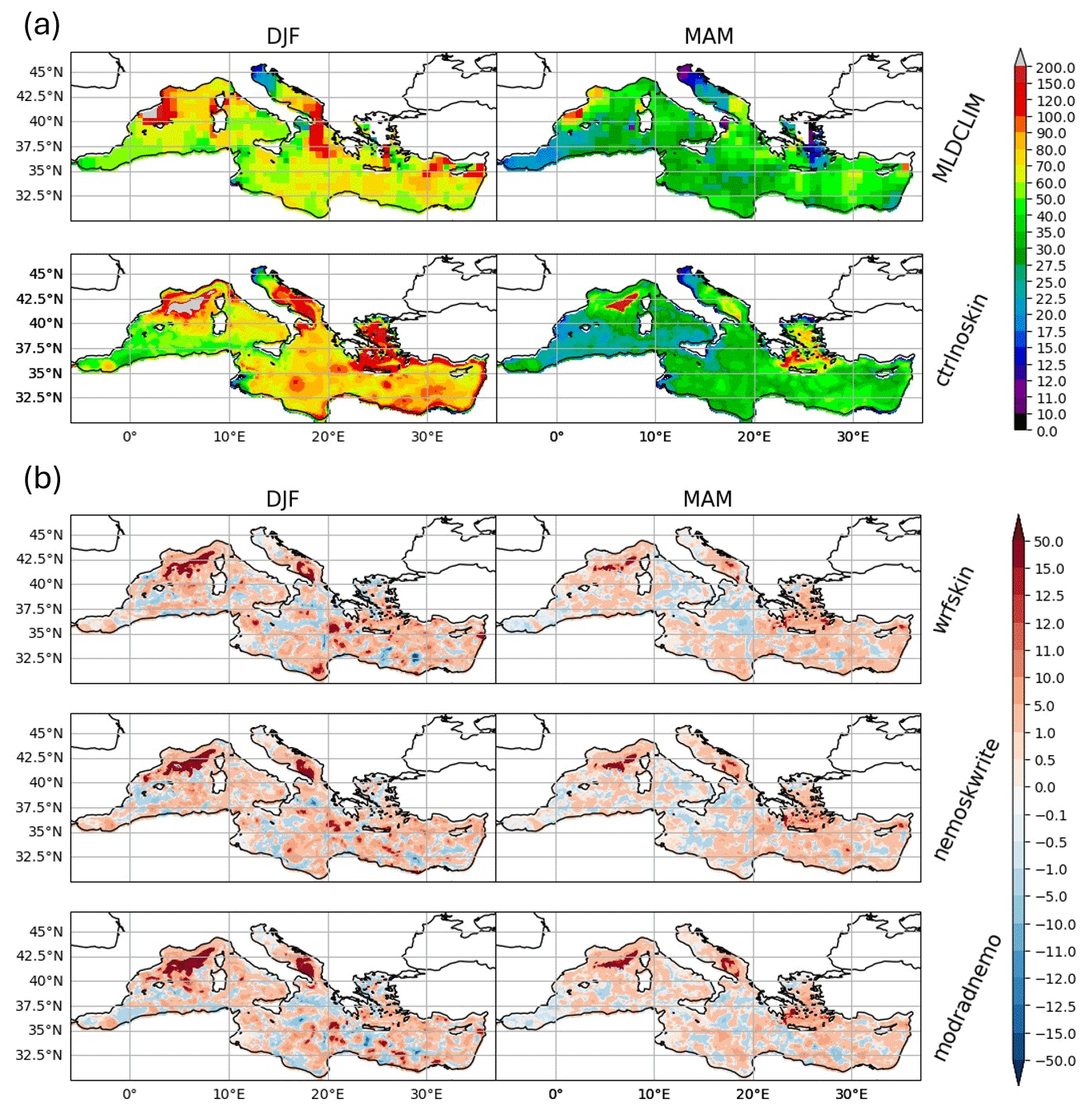
Figure 12 Maps of DJF and MAM of mixed-layer depth for climatology and control simulation are shown in panel (a). Panel (b) shows the difference in the control with respect to each simulation. Values are given in units of metres.

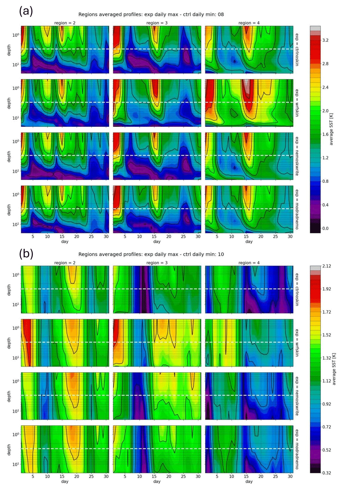
Figure 13 Hovmöller plots for the spatial average of model output temperature profiles in regions 2, 3, 4 as defined in Fig. 11a. Each row shows the difference between daily maxima for the given experiment minus the daily minima for the control simulation. The dashed white line traces the z=3 m line of the depth used as reference for the base of the warm layer as in the ZB05 scheme (Zeng and Beljaars, 2005). Panel (a) shows August, while panel (b) shows October.

Compared to the mixed-layer depth climatology from 1969 to 2013 (Houpert et al., 2015a, b, Sect. 2.7), all of the tested schemes seem to have a similar impact on the seasonality of mixed-layer depth, with larger differences with respect climatological values being mostly located in the eastern Mediterranean Sea and during wintertime and spring (Fig. 12). It may seem from this data that there is not such a huge change when preferring one method over the other considered in this paper, and this may also be because of the short period simulated (2019–2021). Figure 13 shows how our modified scheme allows more (less) vertical propagation of the diurnal signal during summer (winter) with respect to schemes with constant e-folding depth in all central regions of the Mediterranean domain (regions 2, 3, 4 as defined in Fig. 11a) when all of them are referenced to the control simulation temperature daily minimum.

Indeed, from Fig. 13b we can see that when all the temperature profiles for each simulation are referenced to the ctrlnoskin daily minimum, there is a much wider diurnal warming signal for most of all the considered depth levels, with modradnemo representing an intermediate situation between the wrfskin and the nemoskwrite simulations. This is probably due to the inclusion of chlorophyll-interactive variations, which allow for a better representation of the variability in the mixed-layer dynamics.

Estimates of the mean Mediterranean heat exchange between ocean and atmosphere based on previous studies range from −11 to +22 W m⁻², with an evident dominance of negative estimates, i.e. heat loss from the ocean to the atmosphere (Jordà et al., 2017; Pettenuzzo et al., 2010). Some other studies suggest that the Mediterranean heat budget is close to a neutral value, −1 W m⁻² (Ruiz et al., 2008) or +1 W m⁻² (Criado-Aldeanueva et al., 2012). Many factors can contribute to such wide variability among different estimates, such as differences in the parameterisations employed; initial and boundary conditions; and the way the physical processes, especially through the Strait of Gibraltar, are modelled (Macdonald et al., 1994; Gonzales, 2023).

Table 3 Averaged surface net heat flux over the Mediterranean Sea (W m⁻²): seasonal and annual spatial averaged mean values.

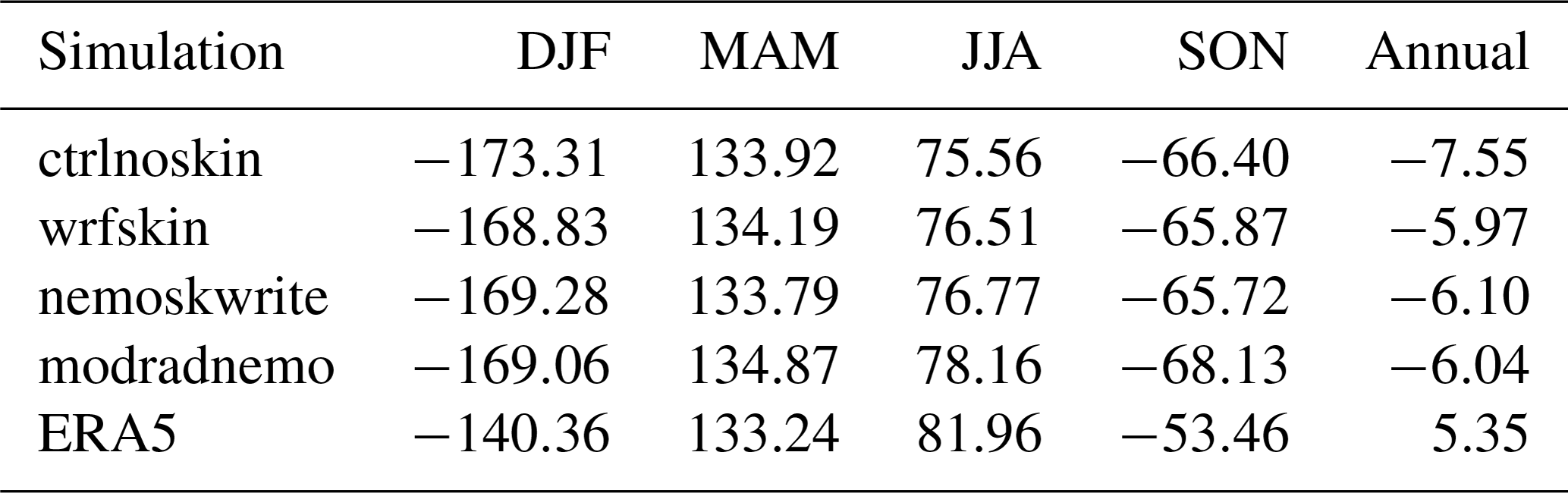
As shown by Table 3, all simulations on an annual basis give a negative, non-closed balance for the net surface heat flux, and modifications to include skinSST, performing very similarly one to another, bring the budget by 1.5 W m⁻² closer to zero, while ERA5 data show a positive net surface heat flux close to 5 W m⁻². However, all estimates fall into the (large uncertain) literature-based estimates. On seasonal timescales, the inclusion of skinSST diurnal variations has the following effects:

• less net heat loss to the atmosphere during wintertime with respect to the control run (wrfskin differing from the ctrlnoskin by about 6 W m⁻², while nemoskwrite and modradnemo having a similar impact, with a difference of about 4 W m⁻² with respect to the control run);

• in springtime, all simulations show a positive imbalance, with the highest difference with respect to the control run of about 1 W m⁻² in the modradnemo simulation;

• during summer, our modified scheme brings on average about 3 W m⁻² more than the control simulation into the basin, yielding an estimate which is closer to ERA5;

• in autumn, our scheme cools down more than the control (about 2 W m⁻²), being the farthest simulation from ERA5 estimate, while traditional schemes tend to have a less negative net heat input.

All seasons except spring show larger difference with respect to ERA5 fluxes, with underestimation in summer and overestimation during winter and autumn, resulting in a bias of about 10 W m⁻² with respect to the net heat flux annual budget in ERA5.

5 Summary and conclusions

In this paper we studied the sensitivity of a regional coupled ocean–atmosphere–hydrological discharge regional model of the Mediterranean Sea to prognostic schemes for skin sea surface temperature. Specifically, we developed a new scheme that allows for spatial and temporal variations in the warm layer's extent according to seawater's transparency conditions. This is possible using tabulated solar extinction coefficients already used in the ocean model and inverting the functional form, which determines how the solar radiation varies along the vertical direction to find the depth at which this latter drops to $\mathrm{1}/e$ from its surface value.

We simulated the period 2019–2021, analysing hourly model outputs and comparing aggregated results with satellite, objectively analysed, and drifter data. Overall, the comparison with data shows that the new scheme improves what is already implemented in NEMO; e.g. mean diurnal warming amplitudes are closer to satellite observations in winter, spring, and autumn, not being much worse than other existing schemes in summer, at least when looking at maps of mean diurnal warming amplitude grouped by seasons. Looking to the typical temperature profile in both the eastern and the western Mediterranean Sea, non-negligible differences across schemes stay confined in the topmost 20 m (100 m) depth during summertime (wintertime). Regionally, typical profiles are warmer than EN4 observation year-round for western regions (regions −1, 1, 2), especially in winter, while regions in the east show a smaller RMSE in the topmost metres for basically all the regions and months when comparing modradnemo to nemoskwrite. The Adriatic Sea has a systematically higher RMSE with respect to EN4 in all the tested methods for the whole period considered. In the central regions, the new scheme penetrates temperature anomalies more (less) during summer (winter) months, having a less intense mean diurnal warming amplitude signal in summer, especially over the upper few metres (the converse holds for wintertime values). Therefore, with respect to the ctrlnoskin simulation, nemoskwrite shows the coldest signal, wrskin the hottest signal, and our modification modradnemo constitutes the middle situation, with a milder summer and winter than the control run. Our interpretation is that within modradnemo, the Chl-interactive e-folding depths allow, where and when necessary, the warm layer to become a little deeper than in the already existing scheme (nemoskwrite), depending on Chl variations. For these space–time points, solar penetration is increased, and thus it tends to make the warm layer warmer. Therefore, future research efforts should be devoted to the better characterisation of this aspect, especially to understand if the modified vertical penetration of heat has some particular effect on the dynamics of the mixed layer (see Song and Yu, 2017, and references therein).

Furthermore, testing the implementation within NEMO of more sophisticated radiative transfer models (such as the one of Ohlmann and Siegel, 2000) or the development of deep-learning-based parameterisations are underway as future research efforts. On a long-term perspective, the method needs to be tested also in other areas and for longer periods, which can increase the results' certainty and allow for usage in investigating impacts on relevant climate large-scale phenomena, where the role of an improved diurnal warming signal could be more relevant (Bernie et al., 2007, 2008). These include phenomena and physical processes such as propagation of marine heat waves (MHWs) or deep-water formation and deep convective events.