rSHUD v2.0: advancing the Simulator for Hydrologic Unstructured Domains and unstructured hydrological modeling in the R environment

Hydrological modeling is a crucial component in hydrology research, particularly for projecting future scenarios. However, achieving reproducibility and automation in distributed hydrological modeling research for modeling, simulation, and analysis is challenging. This paper introduces rSHUD v2.0, an innovative, open-source toolkit developed in the R environment to enhance the deployment and analysis of the Simulator for Hydrologic Unstructured Domains (SHUD). The SHUD is an integrated surface–subsurface hydrological model that employs a finite-volume method to simulate hydrological processes at various scales. The rSHUD toolkit includes pre- and post-processing tools, facilitating reproducibility and automation in hydrological modeling. The utility of rSHUD is demonstrated through case studies of the Shale Hills Critical Zone Observatory in the USA and the Waerma watershed in China. The rSHUD toolkit's ability to quickly and automatically deploy models while ensuring reproducibility has facilitated the implementation of the Global Hydrological Data Cloud (https://ghdc.ac.cn, last access: 1 September 2023), a platform for automatic data processing and model deployment. This work represents a significant advancement in hydrological modeling, with implications for future scenario projections and spatial analysis.

1 Introduction

Scientific modeling utilizes mathematical equations representing natural laws to predict unknown variables in space and time by incorporating known variables (Beven, 2012; Duffy, 2017). Hydrological modeling remains crucial for analyzing future scenarios and for hypothesis testing. As hydrological models evolve from lumped to distributed models, the need for spatial data in modeling continually rises. Simultaneously, with the advancement of numerical methods as computation strategies in hydrological modeling, the models pose new challenges for hydrological unit partitioning (Paniconi and Putti, 2015; Peckham et al., 2017; Peel and McMahon, 2020).

Many hydrological models rely on graphical user interface (GUI) tools for data pre- and post-processing, such as arcSWAT (Arnold et al., 1998) and PIHMgis (Kumar et al., 2010; Bhatt et al., 2014). The GUI interface tools are definitely user-friendly and easy to use, making them favorable for promoting models. However, there are two common challenges with GUI interface tools. First, poor repeatability due to difficulties in duplicating a user's data editing process leads to modeling discrepancies in the same simulation area. Second, GUI interface tools face difficulties in handling large amounts of modeling tasks. In modeling with GUI tools, human participation is required instead of being controlled via modeling parameters, making it impossible to implement a large number of hydrological modeling cases. For instance, the deep-learning methods' modeling process, which is mainly completed automatically via parameter configuration, allows 671 basins in CAMELS data to be automatically modeled, optimized, and verified (Newman et al., 2017; Beven, 2020; Nearing et al., 2021; Li et al., 2022). However, similar automated modeling, simulation, and analysis work with a distributed hydrological model seems an impossible mission considering that lumped models such as SAC-SMA (Burnash et al., 1973), which are frequently compared with deep-learning models in the research literature, require minimal data pre-processing.

Therefore, when dealing with a large number of watershed simulation tasks, both pre-processing and simulation post-processing necessitate the utilization of intervention-free, reproducible, and automated tools. Hence, the development of automated and reproducible pre-processing and post-processing tools for distributed hydrological models and numerical method hydrological models is imperative. However, regardless of the modeling tools used, it encompasses epistemic uncertainty, affecting the final results and accuracy of hydrological simulations(Beven and Young, 2013; Beven, 2013, 2018, 2019). Various modeling tools can technically support the modeling process but cannot eliminate the inherent uncertainties in models and data. Users need to be vigilant about this.

This paper introduces the rSHUD tool, an open-source toolkit developed in the R environment that supports pre- and post-processing functionalities for the Simulator of Hydrological Unstructured Domains (SHUD) and similar surface–subsurface integrated hydrological models. Its tools can be combined into automated processing scripts suitable for batch modeling, simulation, and analysis tasks.

The article begins by presenting the R environment and the rSHUD package in Sect. 2, followed by a brief introduction of SHUD model structure in Sect. 3. Then the critical steps in deploying the SHUD model using rSHUD tools are described in Sect. 4. Lastly, in Sect. 5, the paper showcases two basins as case studies to demonstrate rSHUD's modeling and results analysis process.

2 R and rSHUD

R, a freely available programming language, is widely utilized for data analysis and statistical computations. Renowned for its extensive core functions and libraries, R supports user-defined functions in multiple languages, including C/C++, Python, and Fortran. Its cross-platform compatibility encompasses Linux/Unix, Mac OS X, and Windows. RStudio (https://rstudio.com, last access: 1 September 2023) is a popular GUI for R. Beyond core libraries, R allows easy integration of additional libraries. Users can swiftly install these from the CRAN repository using install.packages or access developer libraries on GitHub via the devtools:install_github function. The library and require functions enable loading of these packages into the active environment.

In addition, rSHUD is an open-source project available on GitHub (https://github.com/shud-system/rSHUD, last access: 1 September 2023) and regularly updated. Since it is not yet available in CRAN's repository, users can install rSHUD and the necessary libraries in their environment using the devtools library. These two commands install rSHUD and the required libraries in the user environment. The following will install the required libraries and rSHUD in the user environment.

    install.packages("devtools")
    devtools::install_github
    ("SHUD-System/rSHUD")

The rSHUD version matches the SHUD model version. The current version of rSHUD is 2.0, designed to support SHUD v2.0 (Shu, 2023a). To ensure compatibility and streamline user experience, the development team maintains concurrent versioning for both rSHUD and SHUD. While rSHUD is developed using the R programming language, SHUD is implemented in C/C++. The versioning process is managed manually to ensure consistency between the two.

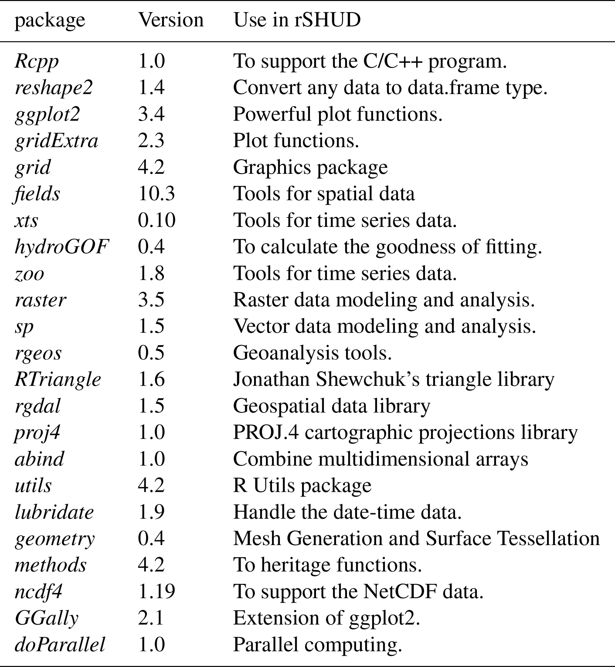
Installation of rSHUD and the dependent library may take some time. The additional R libraries required for rSHUD are listed in Table A1 in Appendix A. The rSHUD package serves several important purposes in the field of geospatial data analysis and hydrological modeling.

• It converts geospatial data to SHUD format. This package is equipped with a toolkit that handles raster and vector data. It then constructs an unstructured triangular mesh domain, which is an important step in preparing SHUD model data.

• It parameterizes the hydraulic properties of soil and land cover. This feature enables users to define and adjust the hydraulic properties of various soil types and land cover classes, improving the applicability of the model.

• It has the ability to read and write SHUD input files. This feature ensures smooth integration with the SHUD model and allows users to import and export data easily.

• It has the ability to load the output results generated by the SHUD model. This facilitates the interpretation and further analysis of the model's results.

• It facilitates hydrological time series and geospatial analysis. This feature allows users to perform detailed temporal and spatial analyzes of hydrological data, providing valuable insight into water dynamics.

• It explores time series and spatial data. This function allows users to generate clear and informative visual representations of their data and helps with data interpretation and communication.

Each function in rSHUD has its own help page that provides information on its usage, arguments and return values. With more than 160 functions included in rSHUD, it is not feasible to provide explanations of all functions in this paper. However, users can access the help page for each function by using the command help(FunctionName).

3 Model and data

3.1 SHUD

SHUD is a distributed hydrological model that is based on physical principles, namely the Saint Venant equation for the surface runoff and Darcy–Richards equation for the subsurface flow (Shu et al., 2020). It solves the partial differential equations (PDEs) of hydrology with the finite-volume method (FVM), which allows for the direct coupling of equations representing groundwater, soil moisture, surface water, vegetation, and land cover interactions. The model's nomenclature, Simulator of Hydrological Unstructured Domains, stems from this intricate process of domain decomposition and the subsequent numerical solution of the associated PDEs within these unstructured hydrological domains. SHUD is an improvement and revision of the Penn State Integrated Hydrologic Model (PIHM) (Qu and Duffy, 2007; Kumar et al., 2010; Bhatt et al., 2014; Yu et al., 2014). Shu et al. (2020) provides a detailed explanation of the differences between the two models.

The SHUD source code, data for three exemplary watersheds, and a straightforward result analysis R script are available on GitHub (https://github.com/shud-system/shud, last access: 1 September 2023) and as referenced in (Shu, 2023a). The three showcased examples include Qinghai Lake and the Heihe headwater in China, along with Cache Creek in the United States. Users can download the source code package, compile the model, and initiate the simulation. After the simulation, users can execute the provided R script within the RStudio GUI to retrieve simulation results, facilitating subsequent analysis and visualization.

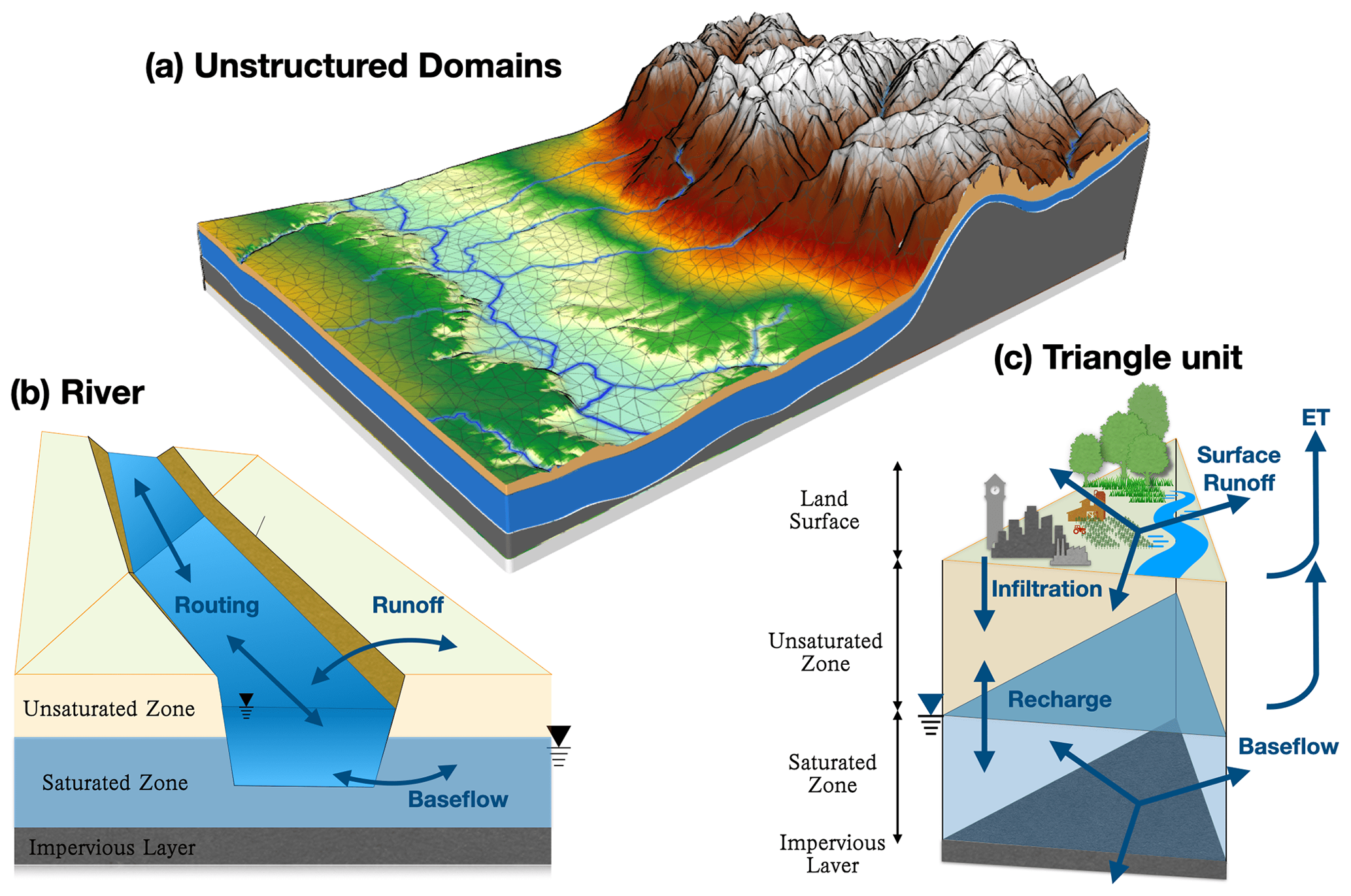
Figure 1 Spatial and hydrological structure of the SHUD model. Unstructured domains in the partial watershed (a), river cells and topological relationships with triangular cells (b), and three-layer triangular prisms (c).

SHUD offers flexibility in terms of time and spatial resolution. The spatial resolution of the model ranges from centimeters to kilometers, depending on the modeling needs and computational resources available. The internal time step, specified by the user as the maximum time step, can be adjusted, while the computing time step is limited to a few seconds. The model exports the status of the catchment at regular time intervals, ranging from minutes to days. Due to its flexibility, the model can be coupled with other systems such as agriculture, cryosphere, ecology, and natural disasters. The SHUD model comprises two types of cells: hillslope and river cells. In the planar view, the hillslope cell has an unstructured triangular shape, while the river cell is portrayed as a rectangle. In the 3D view, the hillslope cell is a triangular prism, and the river cell is a trapezoidal prism (Fig. 1). Both the hillslope and river cells are hydrological computing units (HCUs) in the SHUD numerical solver.

3.1.1 Hillslope cell

The SHUD model utilizes unstructured grids to represent the computing domain of slopes. By default, the Delaunay triangle method is used for building the domain, although other triangular network generation methods are also acceptable. Each triangle comprises three nodes with unique three-dimensional coordinates (x, y, z in meters) that define their location. The centroids of the cells are calculated within the SHUD program. Topological relations are critical to the model and describe the one to three neighbors and nodes associated with each triangle.

For more detailed explanation and mathematical representation, readers can refer to Shu et al. (2020). We will briefly explain the three crucial processes in the watershed hydrology.

• Surface Water Partitioning. While Hortonian and Dunnian overland flows are common assumptions in conceptual models, integrated surface–subsurface hydrological models (ISSHMs) like SHUD adopt a more physical description. Instead of these assumptions, they use the Darcy–Richards equation, such as the Green-Ampt method. In SHUD, surface runoff is calculated using Manning's formula for a hydrological computing units (HCUs).

• Evapotranspiration. Potential evapotranspiration (PET) is computed using the Penman–Monteith equation, while actual evapotranspiration (AET) is derived by multiplying PET with a soil moisture stress coefficient, determined by soil moisture content and groundwater table depth.

• Subsurface flow. Once water infiltrates the ground, it first moves vertically in the unsaturated zone. The flux from unsaturated zone to the saturated zone is termed as “recharge to groundwater”. The calculation of horizontal groundwater flux in horizontal direction is based on the Dupuit assumption.

3.1.2 River cell

In geospace, a river network is a series of sequentially connected polylines that are defined as an ordered set of nodes in three-dimensional coordinates. A river reach is a polyline between two critical nodes. A critical node can be the intersection of multiple rivers or a user-assigned point. Ordinarily, the first node marks the beginning of a reach, while the last node represents its end. The Strahler stream order (Strahler, 1952) in SHUD determines the order of branching of the river system. The triangular domain in SHUD intersects the river network, and the topological relationship between the polylines and triangles determines the exchange of surface and subsurface water between the river channel and hillslope (Shu et al., 2020). The river outlets are typically located at the edge of the watershed.

The topological relationships between the river and hillslope cells are an essential difference between SHUD and PIHM. In the PIHM model, the river network is adjacent to two triangular cells, which results in the following three issues.

1. The length of the river network has an important impact on the number of computing units in both river and hillslope domain. Users need to balance river channel simplicity with the number of computation units; the simplicity implies modification on natural feature of river network.

2. In plain areas, the heavily meandering river network generates hundreds of small triangular cells, easily exceeding the necessary number of HCUs and slowing down model computation dramatically and unnecessarily.

3. The accumulation of water in sink cells violates the fundamental assumption of the shallow surface runoff equation, which consequentially causes the model to become unstable and results in poor performance. At the start point of the first-order stream, the occurrences of local sink points are very frequent and greatly reduce the computational performance of the entire watershed.

To tackle the above issues in PIHM, a modeler need to manually modify the shape of the river channels repeatedly, which reduces the efficiency and reproducibility of modeling. Accordingly, the river network of the SHUD model is superimposed upon triangular cells. This configuration facilitates the computation of groundwater exchange between hillslopes and the river network, which is determined by the hydraulic gradients existing between the river channel and the groundwater level. Meanwhile, surface fluxes are calculated utilizing the weir flow equation (Shu et al., 2020).

3.1.3 Vertical layers

SHUD defines three vertical layers for each hillslope cell (Fig. 1(c)): the land surface, the unsaturated layer (vadose zone), and the saturated layer (groundwater). By default, the model assumes that the no-flow boundary at the bottom is an impervious layer, also known as the impervious bedrock layer.

Thus, the model's default settings define three elevations: the land surface (z_s), the groundwater table (z_g), and the bedrock (z_b). The water stored above z_s is called surface ponding water, while the water between z_g and z_b is known as groundwater. The elevations of z_s and z_b remain constant for each cell, whereas z_g fluctuates based on groundwater storage. The space between z_s and z_g is known as the vadose zone. If z_g rises enough to meet z_s, then the vadose zone disappears.

3.2 Raw data

Hydrological models are a combination function that accepts certain input data and parameters and then produces their output. For modelers, the first questions are what data do we need for a hydrological model and what results do we get from the model?

The rSHUD package utilizes three primary types of data: spatial data, time series data, and attribute data.

• Spatial data. This type encompasses a variety of geospatial elements such as elevation, soil classes, land cover classes, meteorological stations and coverage, the boundary of a research area, and the stream network. Spatial data can be in either vector or raster format, both of which effectively represent spatial heterogeneity.

• Time series data (TSD). This type includes meteorological data (precipitation, temperature, radiation, wind speed, and humidity) and phenological data (leaf area index and snowmelt factor). Hydrologic models, depending on their conceptual and mathematical scheme, are sensitive to the time interval of the forcing (or meteorological) data. For instance, the intensity, duration, and frequency (IDF) of precipitation are critical to models for flood prediction, soil erosion, pollutant monitoring, and so forth. Therefore, for short-term hydrologic events, hourly to daily meteorological data are preferred in process-based models, while long-term trend modeling accepts daily to yearly data in most conceptual or water balance models. Given that the SHUD model employs physical hydraulic equations and depicts hydrologic processes at fine spatial and temporal scales, it is recommended to use sub-daily meteorological data.

  For calibration and validation purposes, the model also requires reference data, which could be observational data, comparable datasets from other models, or data from previous publications.

• Attribute data. This includes the feature of the spatial data, used for generating hydraulic parameters of each soil class, geologic layers, and land cover classes. The required soil texture parameters include the percentage of silt and clay, organic matter content, and bulk density. These parameters are used to calculate the hydraulic parameters, including hydraulic conductivity, porosity, and the α and β values in the van Genuchten equations (Shu et al., 2020).

4 Model deployment

Deploying a hydrologic model involves several basic steps. Figure 2 illustrates the typical workflow of hydrologic modeling in a research region. First, data preparation is required to build a dataset subset for the research area. Second, data pre-processing is necessary to reformat the spatial data and attribute table. Third, the model must be built, generating input files for the hydrologic model. Fourth, the program must be executed to perform the modeling. Finally, post-processing is required to read the output files and analyze the results.

The rSHUD package aims to support the three out of five steps in the model deployment: data pre-processing, building the model, and post-processing.

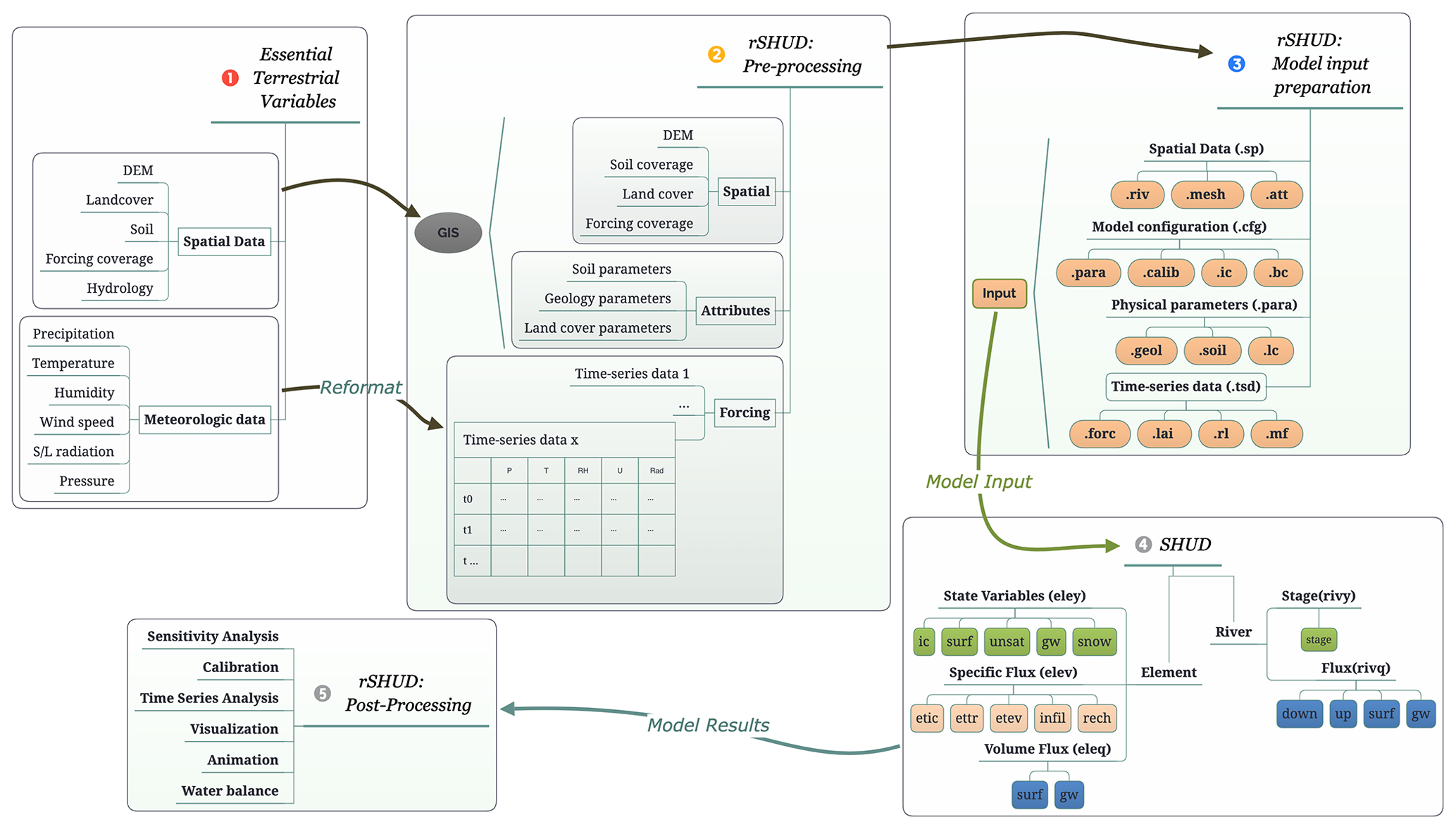
Figure 2 The general workflow of hydrological modeling and implementation of SHUD modeling system, which includes five steps: raw data accessing, pre-processing, and building of the model.

4.1 Data pre-processing

Multiple data processing stages were involved in this step. Holes were removed, modeling boundaries were projected, and buffer zones were generated in sequential procedures. Irrelevant data from the digital elevation model (DEM) were excluded, retaining only pertinent information within the study area. The DEM data underwent reprojection and simplification into a projected coordinate system to facilitate analysis. The river flow direction consistency for the river network data was verified and corrected, while duplicate points and segments were eliminated, and the data format was standardized.

The data pre-processing stage included reformatting the spatial data into a consistent format and generating hydraulic parameters based on the land cover, soil, and geology classification. Prior to data pre-processing, sufficient spatial data were ready, including DEM, soil, land cover, watershed boundary, and river network. As the SHUD model requires a specific format for the time series data, the forcing and phenology data format and units must be standardized. The data type of time series in R is xts. The xts data class supports a matrix format, where rows represent time and columns represent multiple variables. For example, when saving meteorological forcing data, the columns of the data represent precipitation, temperature, wind speed, radiation, and air pressure. Regardless of the original format of the user's data, they can be saved as the data format required by the SHUD model through the write.tsd function. The output file of the write.tsd function is self-explanatory, and users can use other software or programs to save it in other time series data formats.

Consistency of spatial coordination in data processing is indispensable to ensure accurate and reliable results. It is necessary for spatial data to have uniform projection information, which basically means a defined coordinate system. Analysis tools usually accept data either from a geographic coordinate system (GCS) or a projected coordinate system (PCS), a method to represent GCS on a flat surface. However, for hydrological modeling, data in different projections should be re-projected into a specific PCS before spatial processing. This is important since crucial spatial information from maps, including distance (in meters), direction, and area (in square meters), varies across different PCS. It is necessary to ensure the accurate overlay of data from multiple sources to prevent potential spatial inconsistencies.

It is recommended to use the Albers Equal Area projection, which has two reference latitudes and one central longitude. The reference latitudes are set at 25 % and 75 % of the watershed latitude range, respectively. Additionally, the central longitude corresponds to the longitude of the watershed centroid. An example is provided in Sect. 5.

Typically, the extent of the raw spatial data exceeds the watershed boundary; therefore, it is necessary to subset the data. Moreover, the final boundary of the modeling domain may differ from the original watershed boundary because spatial processing simplifies it. Thus, the subset should be slightly larger than the research area. A enclosure mask layer is generated from the watershed boundary with a buffer distance.

The original attributes in the soil data include soil texture components such as silt, sand, and clay percentages, as well as bulk density and organic matter content. To derive hydraulic parameters such as hydraulic conductivity, porosity, and van Genuchten parameters, a pedotransfer function is used based on the soil texture data (Wösten et al., 2001; Shu et al., 2020). Pedotransfer functions (PTFs), being empirical equations derived from specific regional laboratory data, inherently possess limitations in their universal applicability. Users have the flexibility to select and implement alternative PTFs. The primary value of PTFs in rSHUD is to offer an initial estimation of essential hydraulic parameters, while uncertainties in these parameter values should be considered. The pedotransfer function used in rSHUD is listed in Appendix C.

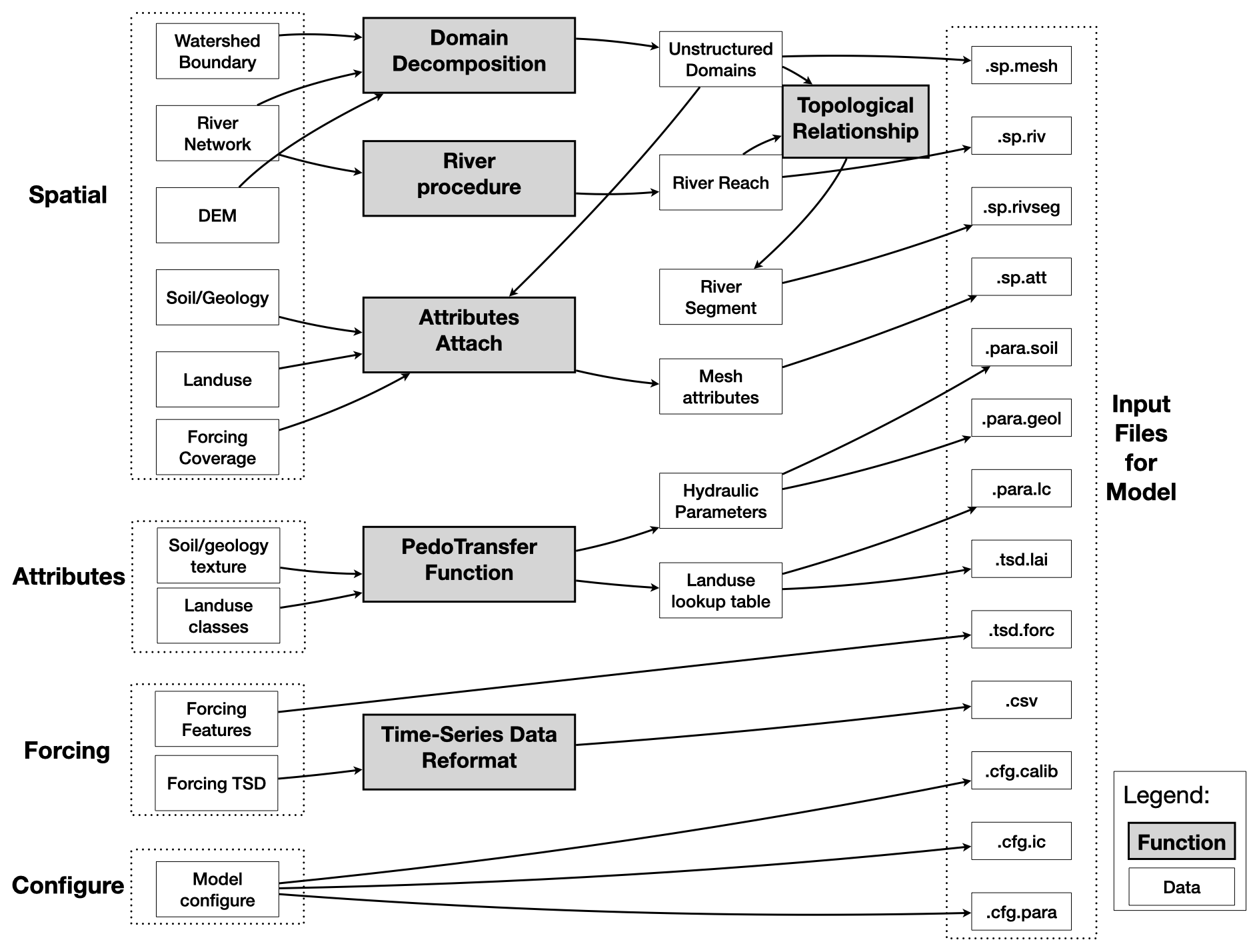
Figure 3 The procedures of model building and the outputs files of rSHUD. The left-hand dashed boxes are input raw data and the right-hand dashed boxes are model input files.

4.2 Model build

4.2.1 Domain decomposition

Domain decomposition is a mathematical strategy that employs geometric principles to partition a larger domain into smaller, more manageable subdomains. Within the context of the SHUD model, this approach is implemented to decompose the watershed into a triangular irregular network (TIN). As a result, the watershed is composed of a collection of unstructured triangles.

The SHUD model can use regular triangles as the computational domains, but unstructured domains are recommended. Unstructured domains offer more flexibility to represent the irregular watershed boundary and terrain features. Moreover, unstructured domains allow for different resolutions within a watershed. For example, modelers can apply coarse TINs in the whole watershed but finer TINs in the river corridor when the research topic concerns surface–subsurface water exchange along the corridor. The multi-resolution configuration ensures sufficient resolution in the area of interest while maintaining the mass balance of the watershed, without increasing the number of HCUs excessively as in regular grid domains.

The triangulation method shud.triangle in rSHUD package is from RTriangle, an R port of Jonathan Shewchuk's Triangle library (Shewchuk, 1996, 2002). The RTriangle generates Delaunay triangles with no small or large angles and is thus suitable for finite-element or volume analysis. The shud.triangle function requires watershed boundary as the mandatory input argument while DEM, river network, islands or holes, and suggesting points are optional conditions to constrain the triangulation. The additional spatial data inserted during the triangulation process allows users to adjust the resolution of HCUs in different areas according to their research needs and study area characteristics, enhancing the flexibility of domain decomposition. There are three extra arguments in RTriangle::triangulate() that are useful to build the ideal domains: the minimum angle of a triangle (argument q), the maximum of triangle's area (argument a), and the ideal number of triangles (argument S).

Prior to performing triangulation, the boundary must be simplified using a tolerance. This process aids in smoothing the watershed boundary while ensuring an appropriate number of HCUs. For instance, when applying watershed delineation methods to retrieve the boundary of a watershed using a 30 m DEM, the resulting boundary often exhibits jagged 30 m scale edges. Therefore, in triangulation, the maximum edge of a triangle on the boundary is limited to 30 m, while the inner portion of the mesh domain is composed of larger triangles. Consequently, the substantial difference in triangle area between the edges and inner parts significantly slows down model performance by unnecessarily increasing computations on the boundary. This negative impact on model efficiency must be addressed by simplifying the boundaries. Simplification is also necessary for additional triangulation constraints such as a river, lake, and urban areas.

After triangulation, the shud.mesh function generates a mesh file that defines triangles by the index of three vertices and three neighbors and the definition of all vertices in the domains (x, y, z coordinates). The definition of TINs can be converted into a text mesh file by shud.mesh, which inversely can then be interpreted into a Shapefile of polygons by a GIS function called sp.mesh2Shape. These functions can cross-validate the consistency of the mesh domain.

4.2.2 River

The processing for the river is to (1) simplify the river reaches, (2) build the flow path, (3) determine the river order, (4) extract the slope characteristics, and (5) describe the geometry of river reach. These functions are integrated into the shud.river function, the functions also can be called independently.

1. The simplification of the river reaches includes two meanings: the one is to simplify the meandering rivers straight, which is optional in SHUD; the other is to cut the very long river reaches into smaller pieces.

2. In GIS and geomorphology, building a river path involves building the connections between upstream and downstream river lines. These connections form the river network and represent how water flows along the river lines. The direction of the river lines determines the inflow and outflow between two rivers. The function is realized by combining sp.RiverDown and sp.RiverPath.

3. River order is a categorization method used to understand the structure of a river network based on the levels of branching within it. The Strahler method (Strahler, 1952) is a wide approach for calculating river order. It assigns a value of 1 to all headwater streams and then increments the value by 1 for each confluence of two streams of equal order. In cases where two streams of different order join, the higher of the orders of the two joining streams is used. This process is repeated downstream until all streams have an order assigned to them. The calculation of river order based on the Strahler method is performed by using the function sp.RiverOrder.

   The order of river reaches determines the generalized geometry (definition of the trapezoidal shape) and hydraulic parameters (Manning's roughness, Chézy coefficient, and so on) of each river reach, since the strong co-relationship exists among slopes, cross-section geometries, river lengths, contribution areas, river orders, discharge, and so on (Flint, 1974; Kratzer et al., 2006; Downing et al., 2012; Perron and Royden, 2013; Strick et al., 2018; McManamay and DeRolph, 2019). In the default configuration, all river reaches in the same order share the same geometry and hydraulic parameters. When a detailed description of individual river reaches is available, the model can also accept a detailed description for each river reach in the model domain instead of categorization by river order.

4. The slope is a critical parameter used to calculate the fluxes in river routing. It is determined by calculating the gradient between the elevations and distances of the starting and ending points of a river reach.

5. The default geometry of a river cross-section is represented by a trapezoidal shape, defined by the width of the riverbed (w), the slope of the bank (s_b), and the depth of the river channel (D) (Fig. 4). The trapezoidal shape is very flexible and can be simplified to a shape of a rectangle (s_b=0) or a triangle (w=0), depending on the specific case. The hydraulic parameters of the river channel encompass five components: sinuosity coefficient of the river reach, Manning's roughness, weir flow coefficient, conductivity, and thickness of sediment. These parameters are pivotal in dictating open-channel flow and the exchange dynamics between the hillslope and the river reach. Given the inherent uncertainties and the lack of precise values during the initial model deployment, the RiverType function provides default values as an initial guess. However, it is worth noting that users retain the flexibility to modify these values based on their measurements or other reliable sources.

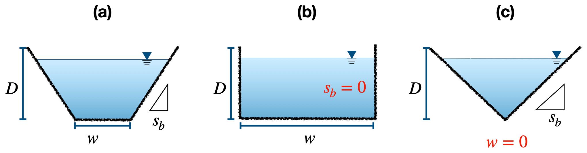
Figure 4 The cross-section of river in the SHUD model, which is described with the width of the riverbed (w), the slope of the bank (s_b), and the depth of the river channel (D). The trapezoidal shape (a) can be simplified to a shape of a rectangle (b) or a triangle (c).

The SHUD model determines the surface–subsurface water flux connections between the river and hillslope cells based on their intersectional relationship. However, the topological relationship between triangles and rivers does not match perfectly. Specifically, a river reach intersects with multiple triangles and exchanges water with these triangular cells. Therefore, to account for the exchange of water, each river reach is divided into several segments, each exchanging water with one triangular cell. The properties of each river segment include the index of the belonging reach, the index of the intersectional triangular cell, and the length of the segment within the cell. The function sp.RiverSeg is used to carry out this task.

4.2.3 Cell attributes

The attribute file contains information about the features of each triangular cell, which is used for hydrological parameters. An example can be found in Fig. 5. The index of soil is used in the .att file to specify a row of parameters in the .para.soil file. Similar to the soil index, the index for geology, land cover, and forcing in the attribute file points to a row in the .para.geol, .para.lc, and .tsd.forc files, respectively.

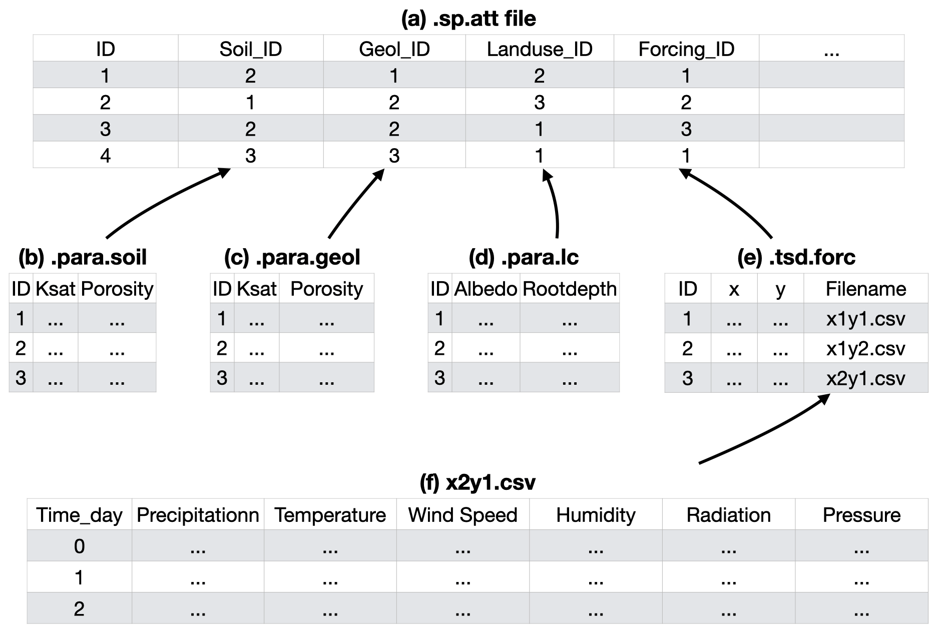
Figure 5 The structure of the model input files and their logical connections. Files represent (a) attributes (.sp.att), (b) hydraulic parameters of soil (.para.soil), (c) geology (.para.geol), (d) land cover (.para.lc), (e) time series of all forcing data (.tsd.forc), and (f) the time series data for specific sites (.csv).

The shud.att function extracts the spatial data index as the properties of each cell. It extracts the features of multiple layers through the centroids of the triangular cells, thus capturing only the value of the centroid instead of the mean or statistical value of the entire cell. For example, a cell contains only one soil type without heterogeneity within the cell. The diversity of soil properties among cells expresses the hydrological heterogeneity in a watershed. Hence, to represent high heterogeneity, a finer resolution of the domain decomposition is required.

4.2.4 Hydraulic parameters

Three main files provide the necessary hydraulic parameters for hydrological simulation: soil, geology, and land cover. The pedotransfer function (Wösten et al., 2001) utilizes soil texture to derive the hydraulic parameters, including vertical and horizontal hydraulic conductivity and porosity, for the deep groundwater layer. Appendix C lists the equations of the pedotransfer functions developed by Wösten et al. (2001).

1. The term “soil” specifically refers to the top layer of soil that influences the infiltration from the surface to the soil and the deep recharge to the saturated layer. The soil layer's essential physical parameters include vertical saturated conductivity, porosity, residual water content, and values α and β for the van Genuchten equation (Shu et al., 2020).

2. The SHUD model's geology layer refers to the aquifer profile's deeper layer. This layer's parameters describe the properties of saturated groundwater flow, and the crucial parameters include vertical and horizontal hydraulic conductivity and porosity.

3. The hydraulic parameters of land cover, such as vegetation root depth, soil degradation ratio, imperviousness factor, and Manning roughness, are stored in a lookup table within the data repository and can be easily transferred to a user's dataset for their modeling efforts. However, it is necessary to note that the lookup table is specifically designed for a particular land cover classification and is not transferable between different classification systems. For instance, the table for the National Land Cover Datasets (Wickham et al., 2020) is not applicable to the USGS 0.5 km MODIS-based Global Land Cover Dataset (Broxton et al., 2014) or the China Land Cover Dataset (Yang and Huang, 2021). Appendix B provides more insight into the default values for multiple land cover classification systems. The University of Maryland (UMD) Global Land Cover Classification (Hansen et al., 2000) determines the parameters for typical land covers based on which the values for other classification systems can be adjusted and transferred. The parameters other than UMD are transferred from UMD data (Hansen et al., 2000; Bhatt, 2012). However, the values in the tables are somewhat arbitrary and act as preliminary values that need to be updated when users have more reliable data. Users can modify the values in the provided lookup tables as needed. If they are employing a different classification system not covered by our default tables, they would need to develop a new lookup table tailored to that system.

4.2.5 Time series data

The .tsd.forc file (Fig. 5) saves a table about the forcing sites, including the x , y, and z of the sites and the time series filename of it (Fig. 5(f)). The SHUD program reads the time series file during the model simulation.

The phenology in SHUD is the leaf area index's (LAI's) TSD, indicating growth, prosperity, and withering. The TSD is also a experiential value for each land cover class from UMD vegetation parameter values (https://ldas.gsfc.nasa.gov/nldas/vegetation-parameters, last access: 1 September 2023).

Similar to the lookup table of land cover parameters, the LAI TSD can be replaced by the user's local observation data.

As the melting factor in SHUD is empirical monthly values for the degree day model calculating the snow melting flux (Hock, 2003; Zhang et al., 2012), the function of MeltingFactor adapts the following equation from Bhatt (2012):

$$\begin{array}{}\text{(1)}& \begin{array}{rl}{M}_{\mathrm{f}}& =\left\{\left({\displaystyle \frac{M_{\max }+M_{\min }}{\mathrm{2}}}\right)+\sin \left({\displaystyle \frac{\mathrm{2}\mathit{\pi }N}{\mathrm{366}}}\right)\right.\\ & \left.\times \left({\displaystyle \frac{M_{\max }-M_{\min }}{\mathrm{2}}}\right)\right\}\times \mathrm{0.4}.\end{array}\end{array}$$

M_f is the melting factor used in the degree day model (mm d⁻¹ K⁻¹). The maximum and minimum values of the melting factor during a year are represented by M_max and M_min, respectively, and occur on 21 June and 21 December. N reflects the Julian day difference from 21 September. As a result, the melting factor follows a sine curve, with its maximum on 21 June and minimum on 21 December. The denominator 366, which represents a leap year, is replaced with 365 for a common year.

In addition, there are boundary conditions (.tsd.bc) and observation data (.tsd.obs) in TSD format, which is optional for the model simulation. The boundary condition may be the irrigation, pumping, leaking, or known water management practices in time series. The optional observation data (.tsd.obs) are generally used for the model calibration only.

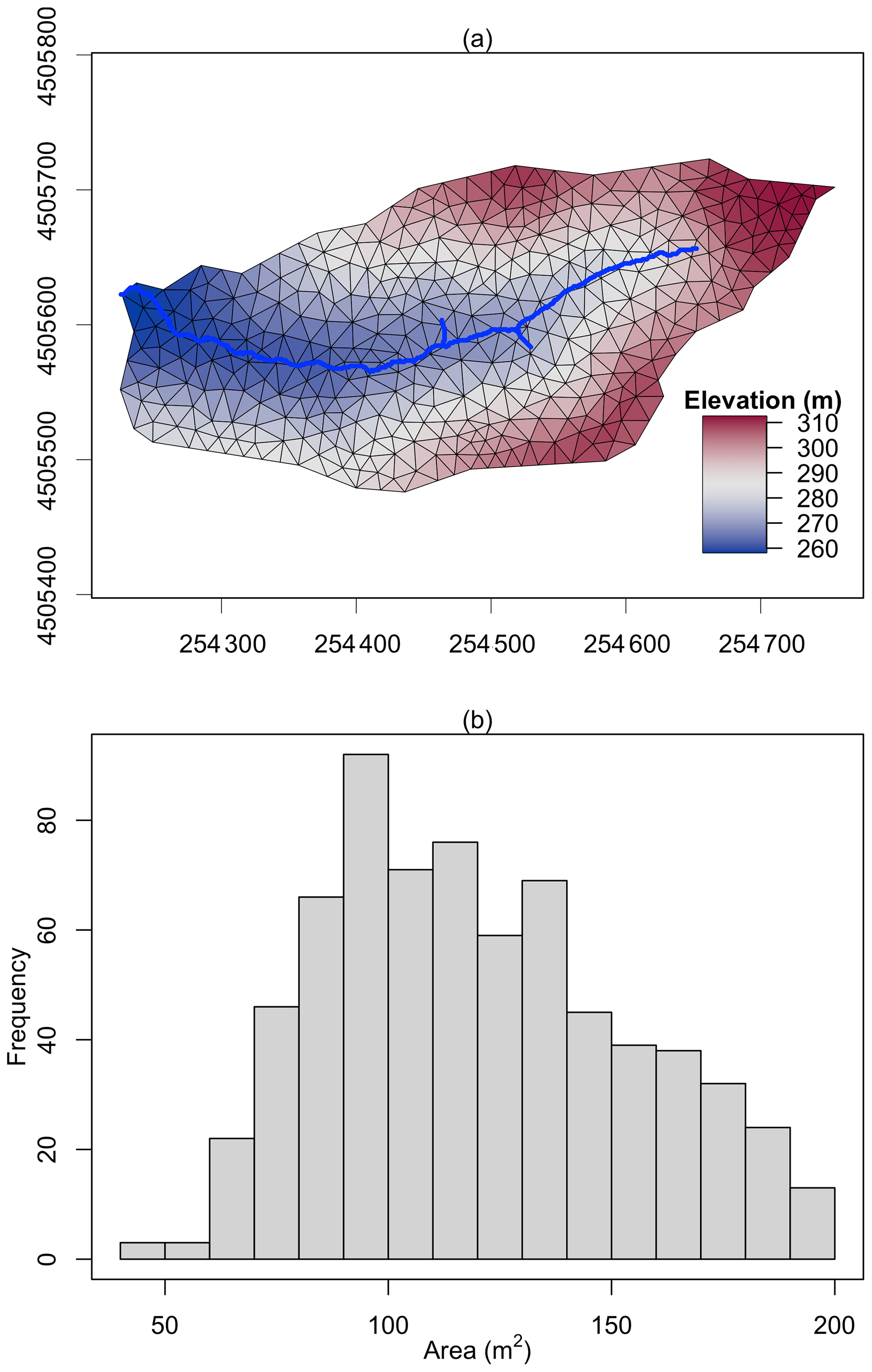
Figure 6 The triangular mesh (a) generated by the function shud.triangle for Shale Hills Critical Zone Observatory (SHCZO), and the histogram of triangle area (b). The color in plot (a) is the centroid elevation of triangles.

4.2.6 Model configuration

In addition to the three primary categories of data – spatial, time series, and attribute data – that hydrologic models commonly require, specific models may also necessitate the inclusion of configuration files. These files define various aspects of the model's operation, establishing the model's running range, determining the level of computational precision, setting the computing and exporting time step, and specifying the file format, among other parameters. Thus, these configuration files provide a means to customize the model's functionality and output to meet specific research tasks and objectives.

(NASA et al., 2018)(Broxton et al., 2014)(Nachtergaele et al., 2008)(He et al., 2020)

Table 1 The description and source of raw data for Waerma watershed.

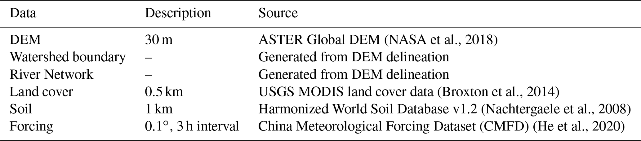
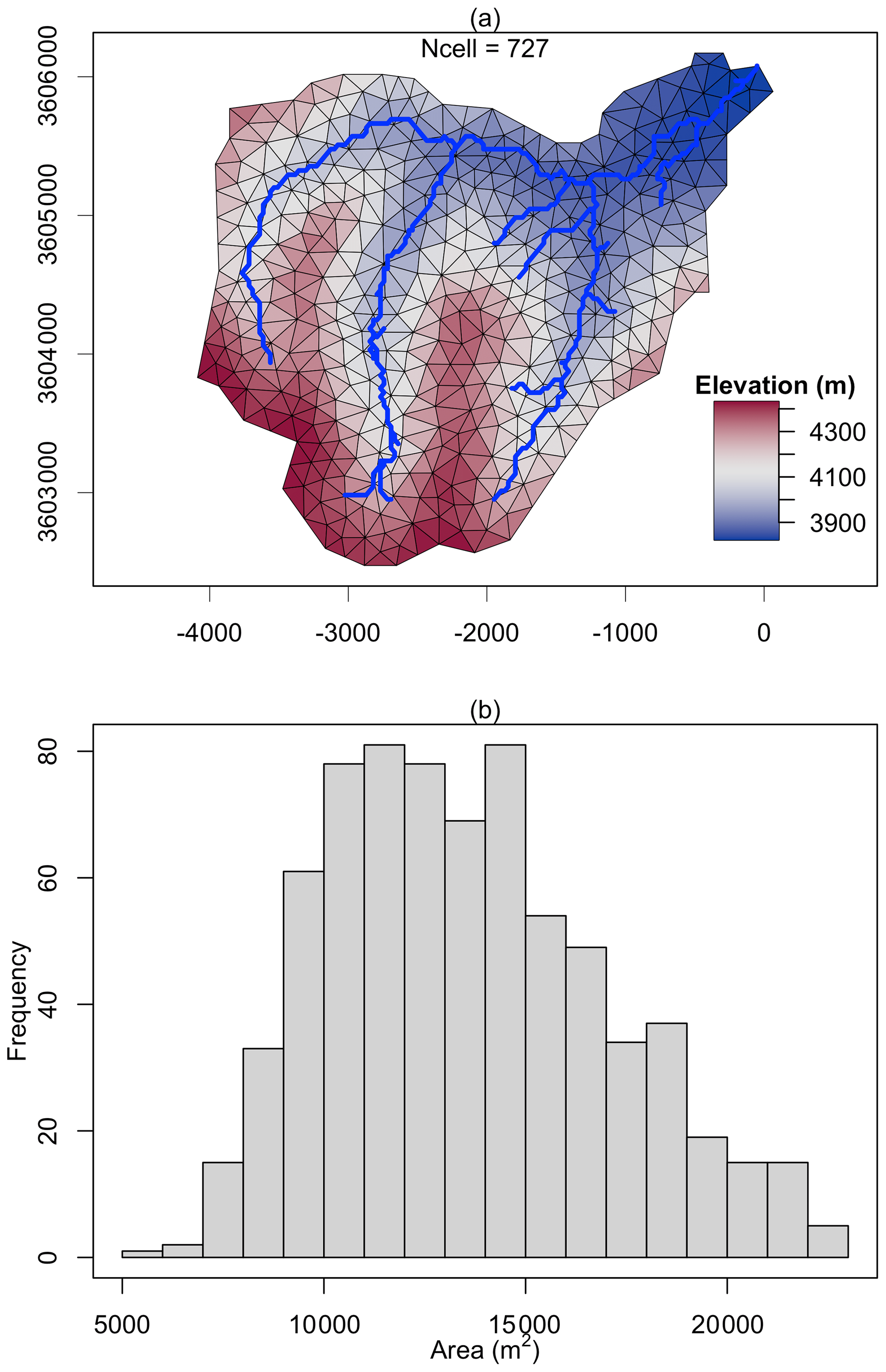
Figure 7 The triangular mesh (a) generated by the function shud.triangle for Waerma watershed and the histogram of triangle area (b). The color in plot (a) is the centroid elevation of triangles.

The SHUD configuration includes four files: the configuration of the simulation (.cfg.para), the calibration file (.cfg.calib), the initial condition of simulation (.cfg.ic), and the boundary condition index (.cfg.bc). To generate boundary conditions with the shud.ic() function, it is necessary to know the index of triangular meshes and river reaches. The indexes in the boundary condition point to specific indexes in the TSD BC files. The initial conditions for river reaches include the initial water level in the channel. Details and file structures of these files are described in the SHUD manual (https://shud.xyz/book_en, last access: 1 September 2023) (Shu, 2019).

5 Examples

To demonstrate the workflow of using the rSHUD package, we chose two watersheds as case studies and gradually implemented the processes of data pre- and post-processing of results. We selected the Shale Hills Critical Zone Observatory (SHCZO) in the USA and the Waerma watershed in China. The rSHUD package already includes all the raw data needed for building the hydrological model, so there is no need to download extra files.

The R scripts for these exemplary watersheds can be found in the Appendices D1, D2, and D3. As the SHCZO is a small and simple catchment, we created a script for the deployment of the SHUD model briefly. The other two scripts (Appendix D2 and D3) are relatively sophisticated for pre- and post-processing the SHUD modeling in the Waerma watershed. All these scripts are embedded in the rSHUD package already. The files demo_sh.R and demo_waerma.R in the rSHUD source code are used to deploy SHUD in the SHCZO and Waerma, respectively, and demo_waerma_ana.R is used for the post-processing of the Waerma watershed. The R scripts are self-explanatory, and users can read the annotations and understand the functionality of the codes. Therefore, we have omitted the details in this paper.

5.1 Shale Hills Critical Zone Observatory in the USA

The Shale Hills Critical Zone Observatory (SHCZO) is a small (≈84 000 m²), forested catchment located in central Pennsylvania, USA. Its topography boasts relatively steep slopes (>0.18) and narrow ridges leading to its Shaver Creek tributary. The elevation of the catchment varies from 250 to 320 m, and it experiences a humid continental climate that averages at 9.5 ^∘C. SHCZO receives an annual mean relative humidity of 65.2 % and precipitation of around 1092 mm. Evapotranspiration is estimated to be 662 mm with an annual runoff of 442 mm, translating to a runoff ratio of about 40 %–50 % (Jin et al., 2011; Shi et al., 2013; Brantley et al., 2018).

All data for the SHCZO modeling are downloaded from the Critical Zone Observatory website (https://czo-archive.criticalzone.org/shale-hills/data/, last access: 1 September 2023). The DEM is 1 m lidar data, and soil is from the local survey (Lin, 2006; Yu et al., 2014). The watershed boundary and river network are calculated from the watershed delineation algorithm in PIHMgis (Bhatt et al., 2014). The local meteorological station provides the forcing variables.

Due to the availability of high-resolution data in this SHCZO and the watershed's small size, a high-resolution SHUD model will be constructed. Since the SHUD model implements a triangular mesh, the triangle's dimensions will vary. We anticipate a maximum triangle area of approximately 200 m². In the result, the function shud.triangle with the constraints produced 698 triangles in SHCZO (Fig. 6). The area of cells within the mesh followed a normal distribution, with values ranging between 40 and 200 m². This distribution highlighted the presence of both smaller and larger triangles within the model.

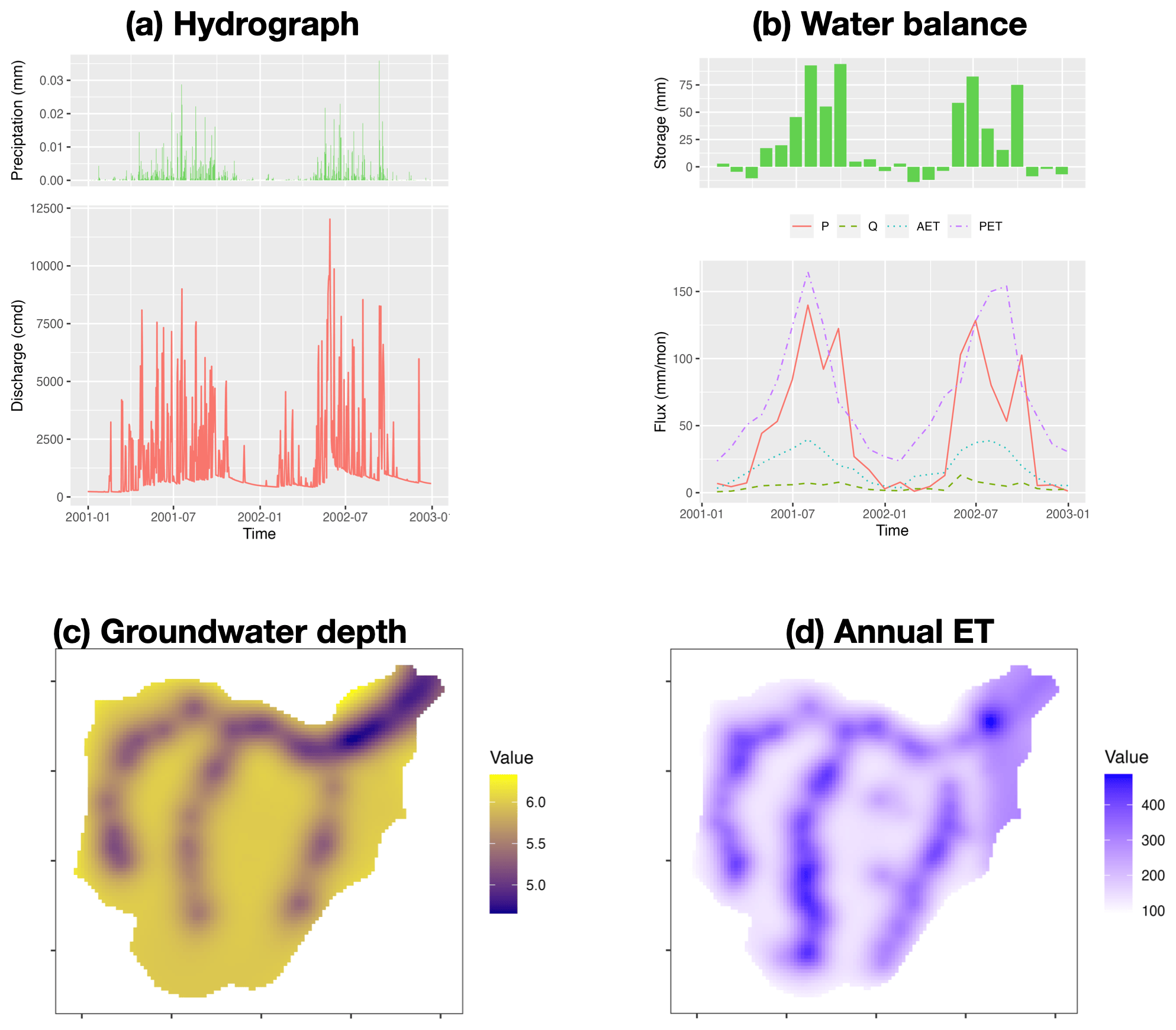
Figure 8 The result analysis of modeling Waerma watershed: (a) hydrograph, (b) watershed scale water balance, (c) groundwater depth (m), and (d) annual evaporation rate (mm yr⁻¹).

The remaining R script of demo_sh.R requires no elaboration as it is easy to read. The code saves all data in a user-specified path. Once data preparation is complete, the SHUD model can be compiled and run. We named the SHCZO project sh. To initiate the simulation on Linux-like platforms, the user should enter ./shud sh. In this example, the forcing data covers 2 years (2008–2009), and the simulation took about 5 min to complete on an Intel 6-Core I5, 64 G RAM computer. While the SHCZO model output closely mirrors the Waerma watershed visualization, Appendix E displays the SHCZO simulation results. This paper's focus is on showcasing rSHUD's capabilities, so detailed parameter optimization for closer alignment with observations was omitted. Consequently, the simulation results serve primarily as a testament to rSHUD's functionality rather than for in-depth analysis.

5.2 Waerma in China

The Waerma watershed is a headwater of the Yellow River, with an area of 9.8 km², located near Waerma Village, about 20 km northwest of Maqu County in Gansu Province, China. It has an elevation of 3800–4500 m with significant terrain fluctuations and an average slope of about 0.42 (rise versus distance). The annual average temperature is about 1.2 ^∘C, and the annual average rainfall is about 630 mm. The main vegetation types are grasslands, meadows, and shrubs. The Key Laboratory of Land Surface Process and Climate Change in Cold and Arid Regions, Chinese Academy of Science, built a comprehensive and detailed observational system for meteorology, land processes, hydrology, and the cryosphere in the Waerma watershed (Meng et al., 2023).

The expected modeling configuration is as follows: using the CMFD data 2000–2001 to drive the SHUD model with larger than 150 m spatial resolution. The maximum triangle area was set to $\mathrm{150}\mathrm{m}\times \mathrm{150}\mathrm{m}=\mathrm{22}\mathrm{500}{\mathrm{m}}^{\mathrm{2}}$; therefore, there is a line a.max = 150*150 in the R script (waerma.sh). The raw data are described in Table 1. These data also can be retrieved via the Global Hydrologic Data Cloud (https://ghdc.ac.cn, last access: 1 September 2023).

5.2.1 Deployment

The script to deploy SHUD in Waerma Watershed is saved in demo_waerma.R, and the watershed data are also available in the source code package. The steps to deploy the SHUD model in Waerma Watershed by rSHUD are listed below.

1. Load the necessary R libraries.

2. Set up and create folders for exporting data and figures.

3. Set up the environment for rSHUD,

4. Read and load this project's raw spatial and attribute data. All the spatial data must be reprojected to an identical PCS in this step.

5. Configure the modeling parameters, including the maximum triangle area, the minimum angle of triangles, tolerance to simplifying watershed boundary and river network, thickness of the aquifer, and number of days in the simulation periods.

   The expected minimum resolution of modeling in Waerma is 150 m; therefore, in triangular mesh, the maximum cell area is about 225 000 m². After the domain decomposition with shud.triangle, 727 triangles are generated (Fig. 8) and mean area of them is 13 544 m² (equivalent to 116 m horizontal resolution).

6. Provide time series data processing, including the forcing data, LAI, and melting factor. In addition, the Thiessen polygons of forcing sites are generated, which provide the matching TSD for each cell. The Thiessen polygons are not utilized for spatial interpolation of meteorological data. They are instead employed to delineate the coverage area for each meteorological station. For instance, if we assume there are N triangles falling within the coverage of the first Thiessen polygon, then the .sp.att file (Fig. 5a) will assign a Forcing_ID of 1 to these N triangles. This indicates that the meteorological forcing data for these N triangles are provided by TSD of the first Thiessen polygon.

7. Attach the attributes of soil, geology, and land cover to the triangular mesh.

8. Build the topological relationship between rivers and triangles.

9. Generate the model configuration files.

10. Write the model input files out.

5.2.2 Result visualization

Once the simulation is complete, we can analyze the results (Shu, 2023b). The script of visualization demo_waerma_ana.R still needs to repeat the first three steps of loading R libraries, setting up folders, and loading the environment.

The shud.env function configures the global variable environment, setting up several default variables for data processing to boost post-processing. The input arguments of shud.env include the project name, the path of model input, and the model output.

After this, we start to load and plot the simulation results. A series of reading functions are available to read the model input files and the output files. The readout function reads the simulation results and returns multi-column time series data, where the index for each column represents the index of HCUs. For example, the TSD for the jth river reach can be found in column j of the streamflow data (.rivqdown), whereas the TSD for the jth triangular cell can be found in column j of the potential evapotranspiration file (.elevetp).

Figure 8 demonstrates the visualization of the hydrograph (precipitation versus discharge), water balance (storage change is equal to precipitation minus evapotranspiration minus discharge), the spatial distribution of groundwater table, and annual mean evapotranspiration. Without calibration with observational data, Fig. 8 shows outputs of preliminary simulation, and the resulting values may not be effective. Since the script to read and plot results is self-explanatory, users can read and modify the code based on their own needs. The script of model deployment and the resulting visualization demonstrate the capability of rSHUD for pre- and post-processing of SHUD modeling.

6 Conclusions

The rSHUD is a toolbox developed in the R environment that supports the pre- and post-processing for the SHUD model.

The rSHUD package provides a set of tools to facilitate the conversion, parameterization, integration, analysis, and visualization of hydrologic data for the SHUD model. The package includes a toolkit for raster and vector data to construct unstructured triangular mesh domains. It also enables defining and adjusting hydraulic properties for soil types and land covers. The package ensures seamless integration with the SHUD model, with the ability to read and write input files and load output results. The package also enables detailed temporal and spatial analyses of hydrologic data and data visualization for easier interpretation.

Uncertainty is crucial in hydrological modeling and must be considered even when using the rSHUD package for model deployment. Users should acknowledge uncertainties in data inputs and model parameters, which may arise from measurement errors, natural variability, or limitations in the package's model structure and parameterization. The equations and data embedded within rSHUD package also introduce uncertainties. Users of the rSHUD package should therefore conduct a thorough uncertainty analysis as a preprocessing step to ensure the reliability and robustness of their modeling outcomes.

The tools in rSHUD not only boost the model deployment and analysis for the SHUD model but also can be used for other spatial analysis and hydrological data processing. The package has more than 160 functions developed in R and keeps growing. Users can type the command ls(”package:rSHUD”) to see a list of all functions available within the rSHUD package and help(FunctionName) to access the function description. An automatic data processing and model deployment platform, Global Hydrological Data Cloud (https://ghdc.ac.cn, last access: 1 September 2023), was implemented with the support of the rSHUD package.

Appendix A: Required R libraries by rSHUD

Table A1 R packages required in rSHUD and their functionalities.

Appendix B: Land cover parameter table

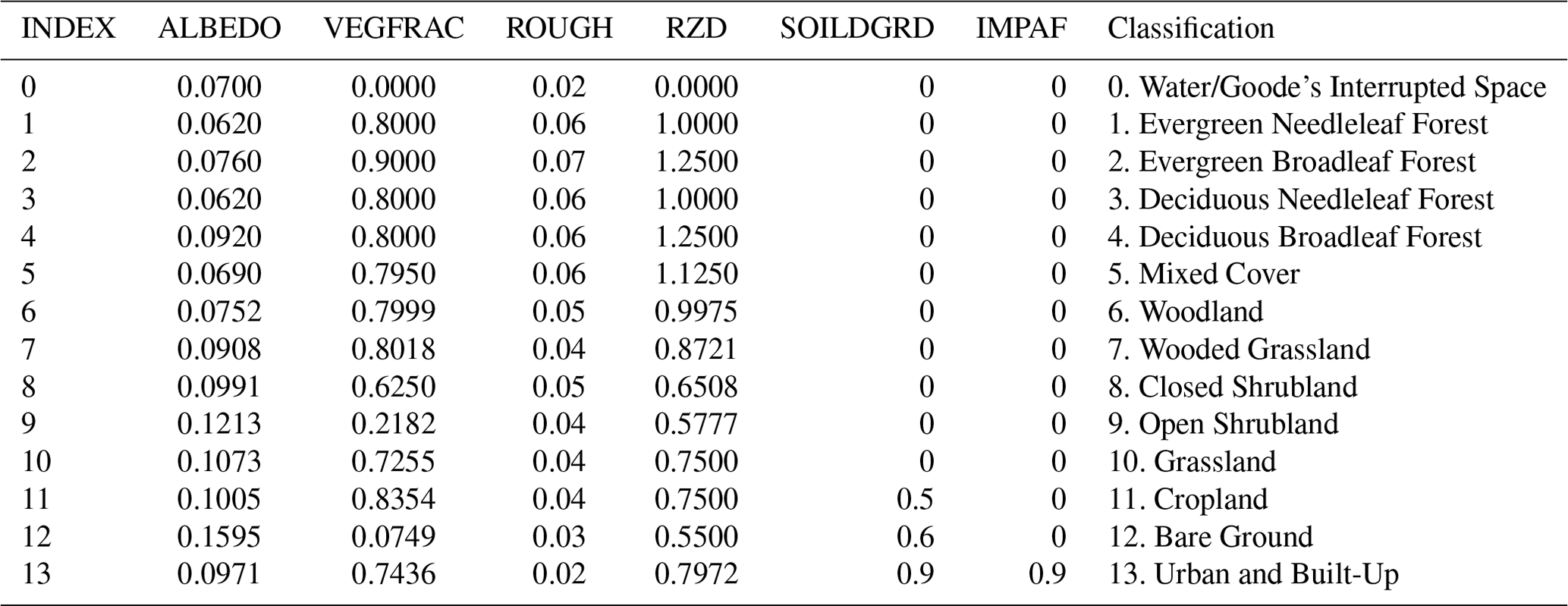
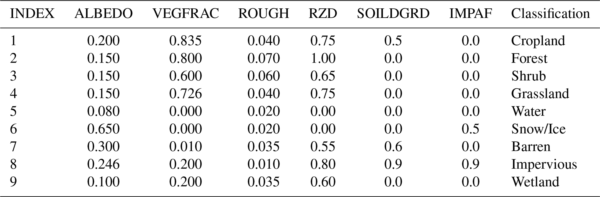
The table headers in this section have specific meanings as delineated below.

• INDEX. This is the index assigned to each row.

• ALBEDO. This refers to the land cover albedo represented as a dimensionless quantity.

• VEGFRAC. This parameter indicates the vegetation fraction and is expressed as a dimensionless quantity.

• ROUGH. This refers to the Manning roughness assigned to the land cover, expressed in units of sm${}^{-\mathrm{1}/\mathrm{3}}$.

• RZD. This is the root depth of the vegetation and is expressed in units of meters.

• SOILDGRD. This parameter indicates the soil degradation ratio, given as a dimensionless quantity.

• IMPAF. This parameter indicates the impervious fraction of the land cover, expressed as a dimensionless quantity.

• Classification. This refers to the name of the classification in its original datasets.

B1 UMD land cover classification

Table B1 The parameters for the University of Maryland (UMD) Global Land Cover Classification (Hansen et al., 2000).

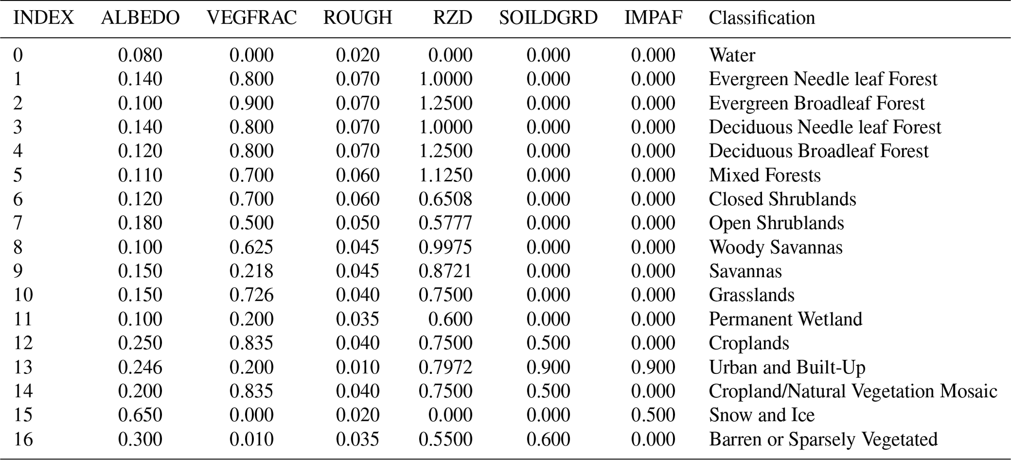
B2 MODIS Global Land Cover

Table B2 The parameters for USGS 0.5 km MODIS Global Land Cover (Broxton et al., 2014).

B3 China Land Cover Dataset

Table B3 The parameters for China Land Cover Dataset (Yang and Huang, 2021).

Appendix C: Pedotransfer function

$$\begin{array}{ll}{\displaystyle }{K}_{\mathrm{sat}}=& {\displaystyle }\exp (\mathrm{7.755}+\mathrm{0.03252}*p_{\mathrm{s}}+\mathrm{0.93}*t_p-\mathrm{0.967}*{\mathit{\rho }}_{\mathrm{b}}*{\mathit{\rho }}_{\mathrm{b}}-\mathrm{0.000484}*p_{\mathrm{c}}*p_{\mathrm{c}}\\ {\displaystyle }& {\displaystyle }-\mathrm{0.000322}*p_{\mathrm{s}}*p_{\mathrm{s}}+\mathrm{0.001}/p_{\mathrm{s}}-\mathrm{0.0748}/p_{\mathrm{om}}-\mathrm{0.643}*\log \left(p_{\mathrm{s}}\right)-\mathrm{0.01398}*{\mathit{\rho }}_{\mathrm{b}}*p_{\mathrm{c}}\\ {\displaystyle }& {\displaystyle }-\mathrm{0.1673}*{\mathit{\rho }}_{\mathrm{b}}*p_{\mathrm{om}}+\mathrm{0.02986}*t_p*p_{\mathrm{c}}-\mathrm{0.03305}*t_p*p_{\mathrm{s}})\\ {\displaystyle }\mathit{\theta }=& {\displaystyle }(\mathrm{0.7919}+\mathrm{0.001691}*p_{\mathrm{c}}-\mathrm{0.29619}*{\mathit{\rho }}_{\mathrm{b}}\\ {\displaystyle }& {\displaystyle }-\mathrm{0.000001491}*p_{\mathrm{s}}*p_{\mathrm{s}}+\mathrm{0.0000821}*p_{\mathrm{om}}*p_{\mathrm{om}}+\mathrm{0.02427}/p_{\mathrm{c}}+=\\ {\displaystyle }& {\displaystyle }+\mathrm{0.01113}/p_{\mathrm{s}}+\mathrm{0.01472}*\log \left(p_{\mathrm{s}}\right)-\mathrm{0.0000733}*p_{\mathrm{om}}*p_{\mathrm{c}}-\mathrm{0.000619}*{\mathit{\rho }}_{\mathrm{b}}*p_{\mathrm{c}}\\ {\displaystyle }& {\displaystyle }-\mathrm{0.001183}*{\mathit{\rho }}_{\mathrm{b}}*p_{\mathrm{om}}-\mathrm{0.0001664}*t_p*p_{\mathrm{s}})\\ {\displaystyle }\mathit{\alpha }=& {\displaystyle }\mathrm{100}*\exp (-\mathrm{14.96}+\mathrm{0.03135}*p_{\mathrm{c}}+\mathrm{0.0351}*p_{\mathrm{s}}+\mathrm{0.646}*p_{\mathrm{om}}\\ {\displaystyle }& {\displaystyle }+\mathrm{15.29}*{\mathit{\rho }}_{\mathrm{b}}-\mathrm{0.192}*t_p-\mathrm{4.671}*{\mathit{\rho }}_{\mathrm{b}}*{\mathit{\rho }}_{\mathrm{b}}-\mathrm{0.000781}*p_{\mathrm{c}}*p_{\mathrm{c}}-\\ {\displaystyle }& {\displaystyle }-\mathrm{0.00687}*p_{\mathrm{om}}*p_{\mathrm{om}}+\mathrm{0.0449}/p_{\mathrm{om}}+\mathrm{0.0663}*\log \left(p_{\mathrm{s}}\right)+\mathrm{0.1482}*\log \left(p_{\mathrm{om}}\right)\\ {\displaystyle }& {\displaystyle }-\mathrm{0.04546}*{\mathit{\rho }}_{\mathrm{b}}*p_{\mathrm{s}}-\mathrm{0.4852}*{\mathit{\rho }}_{\mathrm{b}}*p_{\mathrm{om}}+\mathrm{0.00673}*t_p*p_{\mathrm{c}})\\ {\displaystyle }\mathit{\beta }=& {\displaystyle }\mathrm{1}+\exp (-\mathrm{25.23}-\mathrm{0.02195}*p_{\mathrm{c}}+\mathrm{0.0074}*p_{\mathrm{s}}-\mathrm{0.1940}*p_{\mathrm{om}}+\mathrm{45.5}*{\mathit{\rho }}_{\mathrm{b}}\\ {\displaystyle }& {\displaystyle }-\mathrm{7.24}*{\mathit{\rho }}_{\mathrm{b}}*{\mathit{\rho }}_{\mathrm{b}}+\mathrm{0.0003658}*p_{\mathrm{c}}*p_{\mathrm{c}}+\mathrm{0.002885}*p_{\mathrm{om}}*p_{\mathrm{om}}-\mathrm{12.81}/{\mathit{\rho }}_{\mathrm{b}}-\mathrm{0.1524}/p_{\mathrm{s}}-\mathrm{0.01958}/p_{\mathrm{om}}\\ {\displaystyle }& {\displaystyle }-\mathrm{0.2876}*\log \left(p_{\mathrm{s}}\right)-\mathrm{0.0709}*\log \left(p_{\mathrm{om}}\right)-\mathrm{44.6}*\log \left({\mathit{\rho }}_{\mathrm{b}}\right)-\mathrm{0.02264}*{\mathit{\rho }}_{\mathrm{b}}*p_{\mathrm{c}}\\ {\displaystyle }& {\displaystyle }+\mathrm{0.0896}*{\mathit{\rho }}_{\mathrm{b}}*p_{\mathrm{om}}+\mathrm{0.00718}*t_p*p_{\mathrm{c}})\end{array}$$

where

• K_sat is the saturated conductivity [m s⁻¹];

• θ is porosity of the soil and geology layer [m³ m⁻³];

• α is coefficient in the van Genuchten equation [m⁻¹];

• β is the coefficient in the van Genuchten equation [–];

• p_s is the weight percentage of silt in soil [%];

• p_c is the weight percentage of clay in soil [%];

• p_om is the weight percentage of organic matter in soil [%];

• ρ_b is the bulk density of soil [%];

• t_p is the flag indicating the top or bottom layer: t_p=0, top layer; t_p=1, bottom layer.

Appendix D: R script

D1 Model deployment, Shale Hill CZO

rm(list=ls())
clib=c('rgdal', 'rgeos', 'raster', 'sp', 'fields')
x=lapply(clib, library, character.only=T)

library(rSHUD)
prjname = 'sh'
model.in <- file.path('../demo/input', prjname)
model.out <- file.path('../demo/output', paste0(prjname, '.out'))
fin=shud.filein(prjname, inpath = model.in, outpath = model.out )

dir.create(model.in, showWarnings = F, recursive = T)

load("./data/sh.rda")
wbd=sh[['wbd']]
riv=sh[['riv']]
dem=sh[['dem']]
tsd.forc=sh[['forc']]

# sl = terrain(dem, v=slope, unit='tangent')
# cellStats(sl, quantile)

a.max = 200;
q.min = 33;
tol.riv = 5
tol.wb = 5
aqd=3
NX = 800
years = seq(as.numeric(format(min(time(tsd.forc)), '%Y')),
            as.numeric(format(max(time(tsd.forc)), '%Y')))
ndays = days_in_year(years)


riv.simp = rgeos::gSimplify(riv, tol=tol.riv, topologyPreserve = T)
riv.simp = sp.CutSptialLines(sl=riv.simp, tol=20)

wb.dis = rgeos::gUnionCascaded(wbd)
wb.simp = rgeos::gSimplify(wb.dis, tol=tol.wb, topologyPreserve = T)

# shp.riv =raster::crop(riv.simp, wb.simp)
# shp.wb = raster::intersect( wb.simp, riv.simp)

tri = shud.triangle(wb=wb.simp,q=q.min, a=a.max, S=NX)
# generate  .sp.mesh
pm=shud.mesh(tri,dem=dem, AqDepth = aqd)
sp.mesh=sp.mesh2Shape(pm=pm)
ncell = nrow(pm@mesh)
print(ncell)
# generate  .sp.att

pa=shud.att(tri)

# generate  .riv
pr=shud.river(riv.simp, dem = dem)

# Cut the rivers with triangles
spm = sp.mesh2Shape(pm)
crs(spm) =crs(riv)
spr=riv
sp.seg = sp.RiverSeg(spm, spr)
# Generate the River segments table
prs = shud.rivseg(sp.seg)

# Generate initial condition
pic = shud.ic(nrow(pm@mesh), nrow(pr@river), AqD = aqd, p1 = 0.2, p2=0.2)

go.plot <- function(){
  z=getElevation(pm = pm)
  loc = getCentroid(pm=pm)
  idx.ord = order(z)
  col=colorspace::diverge_hcl(length(z))
  plot(sp.mesh[idx.ord, ], axes=TRUE, col=col, lwd=.5); plot(spr , col='blue',
  add=T, lwd=3);
  # image.plot( legend.only=TRUE, zlim= range(z), col=col, horizontal = T,legend.lab=
  "Elevation (m)",
  #             smallplot= c(.6,.9, 0.22,0.26))
  image.plot( legend.only=TRUE, zlim= range(z), col=col, horizontal = F,
              legend.args = list('text'='Elevation (m)', side=3, line=.05,

               font=2, adj= .2),
              smallplot= c(.79,.86, 0.20,0.4))
}
ia = getArea(pm=pm)
png(filename = '~/sh_mesh.png', height = 9, width = 6, res = 400, units = 'in')
par(mfrow=c(2,1), mar=c(3, 3.5, 1.5,1) )
go.plot();
mtext(side=3, text = '(a)')
hist(ia, xlab='', nclass=20, main='', ylab='')
mtext(side=3, text = '(b)')
mtext(side=2, text = 'Frequency', line=2)
mtext(side=1, text = expression(paste("Area (", m^2, ")")), line=2)
box();
# grid()
dev.off()


sp.c = SpatialPointsDataFrame(gCentroid(wb.simp, byid = TRUE),
                              data=data.frame('ID' = 'forcing'), match.ID = FALSE)
sp.forc = ForcingCoverage(sp.meteoSite = sp.c,  pcs=crs(wb.simp), dem=dem, wbd=wbd)
write.forc(sp.forc@data,
           path = file.path('./input', prjname),
           startdate = format(min(time(tsd.forc)), '%Y%m%d'),
           file=fin['md.forc'])
write.tsd(tsd.forc, file = file.path(fin['inpath'], 'forcing.csv'))

# model configuration, parameter

cfg.para = shud.para(nday=ndays)
# calibration
cfg.calib = shud.calib()

para.lc = lc.NLCD(lc=42) # 42 is the forest in NLCD classes

para.soil = PTF.soil()
para.geol = PTF.geol()

tsd.lai =  LaiRf.NLCD(lc=42, years=years)
write.tsd(tsd.lai$LAI, file = fin['md.lai'])

tsd.mf = MeltFactor(years=years)
write.tsd(tsd.mf, file = fin['md.mf'])
# write  input files.
write.mesh(pm, file = fin['md.mesh'])
write.riv(pr, file=fin['md.riv'])
write.ic(pic, file=fin['md.ic'])

write.df(pa, file=fin['md.att'])
write.df(prs, file=fin['md.rivseg'])
write.config(cfg.para, fin['md.para'])
write.config(cfg.calib, fin['md.calib'])

write.df(para.lc, file=fin['md.lc'])
write.df(para.soil, file=fin['md.soil'])
write.df(para.geol, file=fin['md.geol'])
writeshape(riv.simp, file=file.path(dirname(fin['md.att']), 'riv'))
print(nrow(pm@mesh))

D2 Model deployment, Waerma watershed

rm(list=ls())
# === 1. load library ============
clib=c('rgdal', 'rgeos', 'raster', 'sp', 'fields', 'xts')
x=lapply(clib, library, character.only=T)
library(rSHUD)

# === 2. create directories  ============
dir.prj = '~/Documents/Ex_waerma'
dir.forc = file.path(dir.prj, 'forc')
dir.fig = file.path(dir.prj, 'figure')
dir.create(dir.forc, showWarnings = FALSE, recursive = TRUE)
dir.create(dir.fig, showWarnings = FALSE, recursive = TRUE)

# === 3. setup the project ============
prjname = 'waerma'
model.in <- file.path(dir.prj, 'input', prjname)
model.out <- file.path(dir.prj, 'output', paste0(prjname, '.out'))
fin=shud.filein(prjname, inpath = model.in, outpath = model.out )
if (dir.exists(model.in)){
  unlink(model.in, recursive = T, force = T)
}
dir.create(model.in, showWarnings = F, recursive = T)

# === 4. load and reproject data ============
data(waerma)
wbd=waerma[['wbd']]
meteosite = waerma[['meteosite']] # This is in GCS

crs.pcs = crs.Albers(wbd)
dem = projectRaster(waerma[['dem']], crs=crs.pcs)
wbd= spTransform(waerma[['wbd']], CRSobj = crs.pcs)
riv= spTransform(waerma[['riv']], CRSobj = crs.pcs)

# sl=mask(terra::terrain(dem, opt='slope', unit='tangent'), wbd)
# plot(sl)

r0.soil = waerma[['soil']]
att.soil = waerma[['att']]$soil
rcl.soil=cbind(att.soil[, 1], 1:nrow(att.soil))
r.soil = projectRaster(reclassify(r0.soil, rcl.soil), crs = crs.pcs, method="ngb")

r0.geol = waerma[['geol']]
att.geol = waerma[['att']]$geol
rcl.geol=cbind(att.geol[, 1], 1:nrow(att.geol))
r.geol = projectRaster(reclassify(r0.geol, rcl.geol), crs = crs.pcs, method="ngb")

r0.lc = waerma[['lc']]
att.lc = waerma[['att']]$lc
rcl.lc=cbind(att.lc[, 1], 1:nrow(att.lc))
r.lc = projectRaster(reclassify(r0.lc, rcl.lc), crs = crs.pcs, method="ngb")

# === 5. some threshold for model deployment ============
AREA = 9853260 # KNOWN Area
a.max = 150*150;
q.min = 33;
tol.riv = 50
tol.wb = 50
aqd = 6
NX = AREA / a.max
ndays = 731

# === 6. domain decomposition ============
# simplify the river network.
riv.simp = rgeos::gSimplify(riv, tol=tol.riv, topologyPreserve = T)

# desolve and simplify the watershed boundary
wb.dis = rgeos::gUnionCascaded(wbd)
wb.simp = rgeos::gSimplify(wb.dis, tol=tol.wb, topologyPreserve = T)

# !! Triangulation
tri = shud.triangle(wb=wb.simp,q=q.min, a=a.max, S=NX)
# generate  .sp.mesh
pm=shud.mesh(tri,dem=dem, AqDepth = aqd)
sp.mesh=sp.mesh2Shape(pm=pm)
ncell = nrow(pm@mesh)
print(ncell)

# generate  .riv
pr=shud.river(riv.simp, dem = dem)


# === 7. TSD DATA ============
fns.meteo  =  paste0(meteosite$FILENAME, '.csv')
tsd.forc = waerma$tsd$forc
range(time(tsd.forc[[1]]))
for(i in 1:length(fns.meteo)){
  write.tsd(tsd.forc[[i]], file = file.path(dir.forc, fns.meteo[i]))
}
tsd.mf = MeltFactor(years = seq(as.numeric(format(min(time(tsd.forc[[1]])), '%Y')),
                                as.numeric(format(max(time(tsd.forc[[1]])), '%Y'))))
tsd.lai = waerma$tsd$lai[[1]]
# Coverage of meteorological sites.
sp.forc = ForcingCoverage(sp.meteoSite = meteosite,
                                 filenames= fns.meteo,
                                 pcs=crs.pcs, gcs=crs(meteosite),
                                 dem=dem, wbd=wbd)
write.forc(sp.forc@data, path = normalizePath(dir.forc),
           startdate = format(min(time(tsd.forc[[1]])), '%Y%m%d'),
           file=fin['md.forc'])

# === 8. attributes ============
# generate  .sp.att
pa=shud.att(tri, r.soil = r.soil, r.geol = r.geol, r.lc=r.lc, r.forc = sp.forc)
head(pa)

# === 9. toplogical relation between river and triangle  ============
# Cut the rivers with triangles
spm = sp.mesh2Shape(pm)
crs(spm) =crs(riv)
spr=riv
sp.seg = sp.RiverSeg(spm, spr)
# Generate the River segments table
prs = shud.rivseg(sp.seg)

# Generate initial condition
pic = shud.ic(nrow(pm@mesh), nrow(pr@river), AqD = aqd)

go.plot <- function(){
  z=getElevation(pm = pm)
  loc = getCentroid(pm=pm)
  idx.ord = order(z)
  col=colorspace::diverge_hcl(length(z))
  plot(sp.mesh[idx.ord, ], axes=TRUE, col=col, lwd=.5);
  plot(spr , col='blue', add=T, lwd=3);
  image.plot( legend.only=TRUE, zlim= range(z), col=col, horizontal = F,
              legend.args = list('text'='Elevation (m)',
              side=3, line=.05, font=2, adj= .2),
              smallplot= c(.79,.86, 0.20,0.4))
}
ia = getArea(pm=pm)
png(filename = file.path(dir.fig, paste0(prjname, '_mesh.png')), height = 9,
width = 6, res = 400, units = 'in')
par(mfrow=c(2,1), mar=c(3, 3.5, 1.5,1) )
go.plot();
mtext(side=3, text = '(a)')
mtext(side=3, text = paste0('Ncell = ', ncell), line=-1)
hist(ia, xlab='', nclass=20, main='', ylab='')
mtext(side=3, text = '(b)')
mtext(side=2, text = 'Frequency', line=2)
mtext(side=1, text = expression(paste("Area (", m^2, ")")), line=2)
box();
# grid()
dev.off()

# === 10. configuration files  ============
# model configuration, parameter
cfg.para = shud.para(nday=ndays)

# calibration file
cfg.calib = shud.calib()

para.lc = lc.GLC()
para.soil = PTF.soil(att.soil[, -1])  # only 4 columns
(Silt, clay, OM, bulk density) as input
para.geol = PTF.geol(att.geol[, -1])

# === 11. write  input files. ============
write.mesh(pm, file = fin['md.mesh'])
write.riv(pr, file = fin['md.riv'])
write.ic(pic, file = fin['md.ic'])

write.df(pa, file=fin['md.att'])
write.df(prs, file=fin['md.rivseg'])
write.config(cfg.para, fin['md.para'])
write.config(cfg.calib, fin['md.calib'])

write.tsd(tsd.lai, fin['md.lai'] )
write.tsd(tsd.mf, fin['md.mf'] )

write.df(para.lc, file=fin['md.lc'])
write.df(para.soil, file=fin['md.soil'])
write.df(para.geol, file=fin['md.geol'])
writeshape(riv.simp, file=file.path(dirname(fin['md.att']), 'riv'))
print(nrow(pm@mesh))

D3 Post-processing, Waerma watershed

rm(list=ls())

# === pre1. load library ============
clib=c('rgdal', 'rgeos', 'raster', 'sp', 'fields', 'xts', 'ggplot2')
x=lapply(clib, library, character.only=T)
library(rSHUD)

# === pre2. create directories  ============
dir.prj = '~/Documents/Ex_waerma'
dir.forc = file.path(dir.prj, 'forc')
dir.fig = file.path(dir.prj, 'figure')
dir.create(dir.forc, showWarnings = FALSE, recursive = TRUE)
dir.create(dir.fig, showWarnings = FALSE, recursive = TRUE)

# === pre3. setup the project ============
prjname = 'waerma'
model.in <- file.path(dir.prj, 'input', prjname)
# model.out <- file.path(dir.prj, 'output', paste0(prjname, '.out'))
model.out <- '~/Documents/output/waerma.out'

fin=shud.filein(prjname, inpath = model.in, outpath = model.out )
shud.env(prjname, inpath = model.in, outpath = model.out )
dir.create(model.in, showWarnings = F, recursive = T)

ia=getArea()
ncell=length(ia)
spm=sp.mesh2Shape()

gplotfun <- function(r, leg.lab='value'){
  map.p <- rasterToPoints(r)
  #Make the points a dataframe for ggplot
  df <- data.frame(map.p)
  #Make appropriate column headings
  colnames(df) <- c('X', 'Y', 'Value')
  

  #Now make the map
  g= ggplot(data=df, aes(y=Y, x=X)) +
    geom_raster(aes(fill=Value)) +
    # geom_point(data=sites, aes(x=x, y=y), color=”white”, size=3, shape=4) +
    theme_bw() + coord_equal() +
    # scale_fill_continuous(leg.lab) +
    theme(
      # axis.title.x = element_text(size=16),
      # axis.title.y = element_text(size=16, angle=90),
      # axis.text.x = element_text(size=14),
      # axis.text.y = element_text(size=14),
      axis.title.x = element_blank(),
      axis.title.y = element_blank(),
      axis.text.x = element_blank(),
      axis.text.y = element_blank(),
      panel.grid.major = element_blank(),
      panel.grid.minor = element_blank(),
      legend.position = 'right',
      legend.key = element_blank()
    )
  return(g)
}
gl=list()
# === 1. plot Q (discharge) data ============
oid = getOutlets()
qdown = readout('rivqdown')
prcp = readout('elevprcp')
xt = 1:(365*2)+365*1
q=qdown[xt, oid]
pq = cbind(q, rowMeans(prcp[xt,]))[,2:1]
# gl[[1]] = autoplot(q)+xlab('')+ylab('Discharge (m^3/day)')+theme_bw()
gl[[1]] = hydrograph(pq, ylabs = c('Preciptation (mm)', 'Discharge (cmd)'))
gl[[1]]

# === 2. plot Water Balance ============
xl=loaddata(varname=c('rivqdown', 'eleveta', 'elevetp', 'elevprcp', 'eleygw'))
wb=wb.all(xl=xl, plot=F)[(1:24)+12, ]*1000
gl[[2]] = hydrograph(wb, ylabs = c('Storage (mm)', 'Flux (mm/mon)'), legend.position='top')
gl[[2]]

# === 3. plot groundwater data ============
eleygw = readout('eleygw')[xt, ]
ts.gw=apply.daily(eleygw, sum)/ncell
# plot(ts.gw)
gw.mean = apply(eleygw, 2, mean)
aqd =getAquiferDepth()
r.gw = MeshData2Raster(gw.mean)
d.gw = aqd - r.gw
d.gw[d.gw<0]=0
gl[[3]] =gplotfun(d.gw, leg.lab='Depth (m)')+
  scale_fill_gradient(low = "darkblue", high = "yellow")
gl[[3]]

# === 4. plot ETa data ============
eleveta = readout('eleveta')[xt, ]
ts.eta=apply.monthly(eleveta, sum)
# plot(ts.eta)
eta.mean = apply(eleveta, 2, mean)*365
r.eta = MeshData2Raster(eta.mean)*1000 # mm/day
# plot(spm, axes=TRUE)
# plot(add=T, r.eta)
gl[[4]]=gplotfun(r.eta, leg.lab='Rate (mm/day) ')+
  scale_fill_gradient(low = "white", high = "blue")
gl[[4]]

# === Saving the plots ============
gg=gridExtra::arrangeGrob(grobs=gl, nrow=2, ncol=2)
ggsave(plot = gg, filename = file.path(dir.fig, 'waerma_res.png'),
width = 7, height=7, dpi=400, units = 'in')

for(i in 1:4){
  ggsave(plot = gl[[i]], filename = file.path(dir.fig, paste0('waerma_res_', i,
  '.png')),
         width = 3.5, height=4, dpi=400, units = 'in')
}

Appendix E: Results visualization of SHCZO

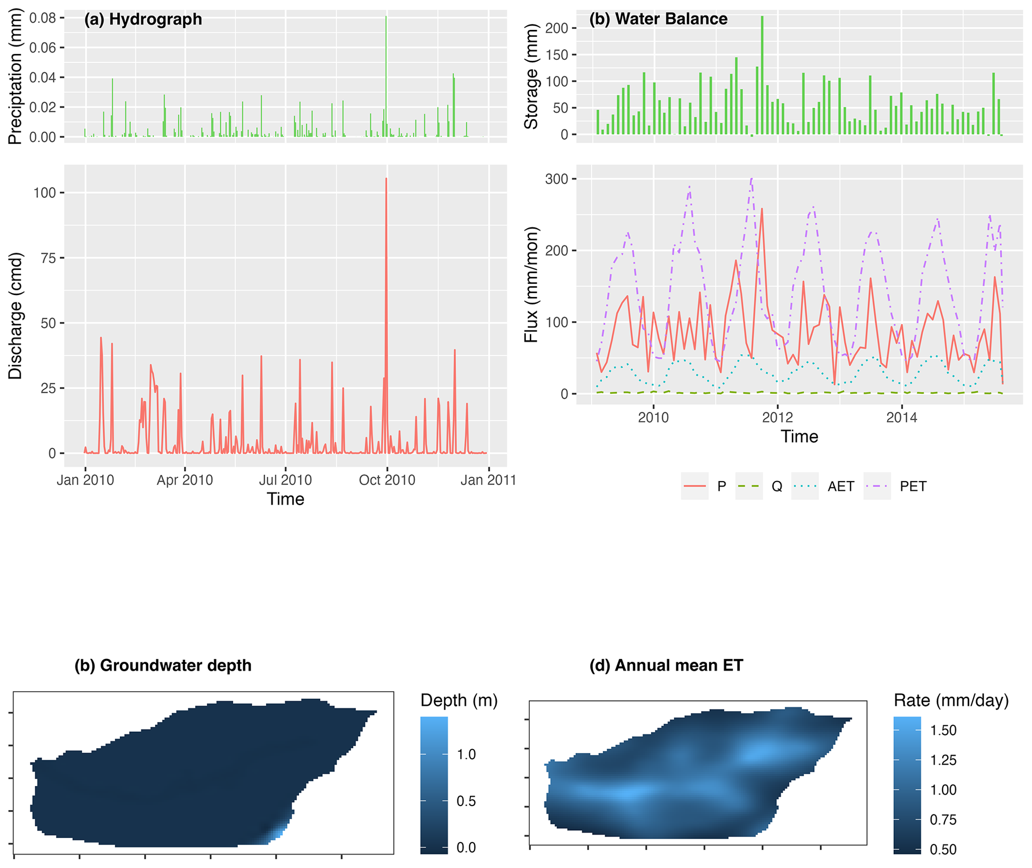
Figure E1 The result analysis of modeling Shale Hills Critical Zone Observatory watershed: (a) hydrograph, (b) watershed scale water balance, (c) groundwater depth (m), and (d) annual evaporation rate (mm yr⁻¹).