A spatiotemporally separated framework for reconstructing the sources of atmospheric radionuclide releases

Determining the source location and release rate are critical tasks when assessing the environmental consequences of atmospheric radionuclide releases, but they remain challenging because of the huge multi-dimensional solution space. We propose a spatiotemporally separated two-step framework that reduces the dimension of the solution space in each step and improves the source reconstruction accuracy. The separation process applies a temporal sliding-window average filter to the observations, thereby reducing the influence of temporal variations in the release rate on the observations and ensuring that the features of the filtered data are dominated by the source location. A machine-learning model is trained to link these features to the source location, enabling independent source-location estimations. The release rate is then determined using the projected alternating minimization with L1 norm and total variation regularization algorithm. This method is validated against the local-scale SCK CEN (Belgian Nuclear Research Centre) ⁴¹Ar field experiment and the first release of the continental-scale European Tracer Experiment, for which the lowest source-location errors are 4.52 m and 5.19 km, respectively. This presents higher accuracy and a smaller uncertainty range than the correlation-based and Bayesian methods when estimating the source location. The temporal variations in release rates are accurately reconstructed, and the mean relative errors in the total release are 65.09 % and 72.14 % lower than the Bayesian method for the SCK CEN experiment and the European Tracer Experiment, respectively. A sensitivity study demonstrates the robustness of the proposed method to different hyperparameters. With an appropriate site layout, low error levels can be achieved from only a single observation site or under meteorological errors.

1 Introduction

Atmospheric radionuclide release is a major environmental concern in the nuclear industry, including in the domains of nuclear energy and applications of the associated heat, isotope production, and the post-processing of radioactive waste. Such releases occurred after the Chernobyl nuclear accident (Anspaugh et al., 1988) and the Fukushima nuclear explosion (Katata et al., 2012), and information on the sources (i.e., the locations) of these releases is incomplete. Recently, there have been several atmospheric radionuclide leaks from unknown sources, such as the 2017 ¹⁰⁶Ru leakage (Masson et al., 2019) and the 2020 ${}^{\mathrm{134}/\mathrm{137}}\mathrm{Cs}$ detection in northern Europe (Ingremeau and Saunier, 2022), which have raised global concerns regarding the subsequent hazard to public health. Identifying source information for these events is critical for the safe operation of nuclear facilities, consequence assessment, and the emergency response.

During these events, source data often cannot be directly measured or determined because of the lack of information on the source of the leak. Instead, source information can only be reconstructed through inversion methods, which identify the optimal solution by comparing the environmental observations with atmospheric dispersion simulations using different estimates of the source location and release rate. Such reconstructions simultaneously identify the source location and release rate because the observations are intuitively determined by both parameters. In this case, the reconstruction searches for a solution over a large multi-dimensional space, where the dimension is the sum of the number of spatial coordinates and the length of the estimated release window. Therefore, the inversion is weakly constrained and can become ill-posed in the case of spatiotemporally limited observations and uncertainties in the atmospheric dispersion models. Unfortunately, this is quite often the case for atmospheric radionuclide releases.

To reduce the problem of ill-posedness, most previous studies have attempted to constrain the reconstruction by imposing assumptions on the model–observation discrepancies or release characteristics. Assumptions about model–observation discrepancies are widely used in Bayesian methods to simultaneously reconstruct the posterior distributions of spatiotemporal source parameters (De Meutter et al., 2021; De Meutter and Hoffman, 2020; Xue et al., 2017a). These assume that the model–observation discrepancies follow a certain statistical distribution (i.e., the likelihood of Bayesian methods), with the normal (Eslinger and Schrom, 2016; Guo et al., 2009; Keats et al., 2007, 2010; Rajaona et al., 2015; Xue et al., 2017a, b; Yee, 2017; Yee et al., 2008; Zhao et al., 2021) and log-normal (Chow et al., 2008; Dumont Le Brazidec et al., 2020; KIM et al., 2011; Monache et al., 2008; Saunier et al., 2019; Senocak, 2010; Senocak et al., 2008) distributions being two popular choices. Other candidates include the t distribution (with the number of degrees of freedom ranging from 3–10), the Cauchy distribution, and the log-Cauchy distribution, all of which were compared against the normal and log-normal distributions in terms of reconstructing the source parameters of the Prairie Grass field experiment (Wang et al., 2017). The results demonstrate that the likelihoods are sensitive to both the dataset and the target source parameters. Several studies have constructed the likelihood based on multiple metrics that measure the model–observation discrepancies in an attempt to better constrain the solution (Lucas et al., 2017; Jensen et al., 2019). More sophisticated methods involve the use of different statistical distributions for the likelihoods of non-detection and detection (De Meutter et al., 2021; De Meutter and Hoffman, 2020). Recent studies have suggested the use of log-based distributions and the tailored parameterization of the covariance matrix as a means of better quantifying the uncertainties in the reconstruction (Dumont Le Brazidec et al., 2021). These Bayesian methods have been applied to real atmospheric radionuclide releases, such as the 2017 ¹⁰⁶Ru event, and have provided important insights into the source and release process (Dumont Le Brazidec et al., 2020, 2021; Saunier et al., 2019; De Meutter et al., 2021). However, these studies have also revealed that in Bayesian methods, the likelihood must be exquisitely designed and parameterized to achieve satisfactory spatiotemporal source reconstruction (Dumont Le Brazidec et al., 2021; Wang et al., 2017). With suboptimal design, the reconstruction may exhibit a bimodal posterior distribution (De Meutter and Hoffman, 2020), which remains a challenge to achieving robust applications in different scenarios.

Assumptions on the release characteristics aim to reduce the dimension of solution space to 4 or 5, namely the two source-location coordinates, the total release, and the release time (or the release start and end time); i.e., it is assumed that there is either an instantaneous release at one time or a constant release over a period (Kovalets et al., 2020, 2018; Efthimiou et al., 2018, 2017; Tomas et al., 2021; Andronopoulos and Kovalets, 2021; Ma et al., 2018). Under these assumptions, the correlation-based method exhibits high accuracy for ideal cases under stationary meteorological conditions, such as synthetic simulation experiments (Ma et al., 2018) and wind tunnel experiments (Kovalets et al., 2018; Efthimiou et al., 2017). However, previous studies have also demonstrated that real-world applications may be much more challenging (Kovalets et al., 2020; Tomas et al., 2021; Andronopoulos and Kovalets, 2021; Becker et al., 2007) because the release usually exhibits temporal variations and may experience non-stationary meteorological fields. In addition, inaccurate calculation of the meteorological field input can further intensify these challenges. The interaction between the time-varying release characteristics and non-stationary meteorological fields is neglected in the instantaneous-release and constant-release assumptions, leading to inaccurate reconstruction.

Given the assumption-related reconstruction deviations in complex scenarios, we propose a spatiotemporally separated source reconstruction method that is less dependent on such assumptions. Our approach reduces the complexity of the source reconstruction using the simple fact that the source location is fixed during the atmospheric radionuclide release process. In this case, the spatiotemporal variations in observations are influenced by the time-varying release rate, source location, and meteorology, among which the last variable is generally known. The proposed method reduces the influence of the release rate through a temporal sliding-window average filter, making the filtered observations more sensitive to the source location than to the release rate. After filtering, existing methods based on direct observation–simulation comparisons may be unable to locate the source. Thus, the response features of the filtered observations are extracted and mapped to the source location by training a data-driven machine-learning model using the extreme gradient boosting (XGBoost) algorithm (Chen and Guestrin, 2016). To fully capture the response features at each observation site, tailored time- and frequency-domain features are designed and optimized using the feature selection technique of XGBoost. Using this optimized model, the source location is estimated based on the filtered observations. Once the source location has been retrieved, the non-constant release rate is determined using the projected alternating minimization with L1 norm and total variation regularization (PAMILT) algorithm (Fang et al., 2022), which is robust to model uncertainties. The sequential spatiotemporal reconstruction reduces the dimension of the solution space at each step, which helps to improve the accuracy and reliability of the reconstruction.

The proposed method is validated using the data from multi-scale field experiments, namely the local-scale SCK CEN (Belgian Nuclear Research Centre) ⁴¹Ar experiment (Rojas-Palma et al., 2004) and the first release of the continental-scale European Tracer Experiment (ETEX-1) (Nodop et al., 1998), which traced emissions of perfluoromethylcyclohexane (PMCH). The performance of the proposed method is compared with the correlation-based method in terms of source-location estimation and with the Bayesian method in terms of spatiotemporal accuracy. The sensitivity of the source-location estimation to the spatial search range, size of the sliding window, feature type, number and combination of sites, and meteorological errors is also investigated for the SCK CEN ⁴¹Ar experiment.

2 Materials and methods

2.1 Source reconstruction models

For an atmospheric radionuclide release, Eq. (1) relates the observations at each observation site to the source parameters:

$$\begin{array}{}\text{(1)}& \mathit{\mu }=F(\mathit{r},\mathit{q})+\mathit{\epsilon },\end{array}$$

where $\mathit{\mu }=[{\mathit{\mu }}_{\mathrm{1}},{\mathit{\mu }}_{\mathrm{2}},\mathrm{\dots },{\mathit{\mu }}_N{]}^T\in {\mathbb{R}}^N$ is an observation vector composed of N observations; the function F maps the source parameters to the observations, i.e., an atmospheric dispersion model; r refers to the source location; q∈ℝ^S is the temporally varying release rate; and ε∈ℝ^N is a vector containing both model and measurement errors.

In most source reconstruction models, F is simplified to the product of q and a source–receptor matrix A that depends on the source location:

$$\begin{array}{}\text{(2)}& \mathit{\mu }=\mathbf{A}\left(\mathit{r}\right)\mathit{q}+\mathit{\epsilon },\end{array}$$

where $\mathbf{A}\left(\mathit{r}\right)=\left[A_{\mathrm{1}}\right(\mathit{r}),A_{\mathrm{2}}(\mathit{r}),\mathrm{\dots },A_N(\mathit{r}){]}^T\in {\mathbb{R}}^{N\times S}$ and each row describes the sensitivity of an observation to the release rate q given the source location r.

2.2 Observation filtering for spatiotemporally separated reconstruction

A straightforward way to solve Eq. (2) is to simultaneously retrieve the source location and release rate; however, the solution space is huge and difficult to constrain. Several studies have noted that the source location can be retrieved separately without knowledge of the exact release rate on the condition that the release rate is constant (Efthimiou et al., 2018, 2017; Kovalets et al., 2018; Ma et al., 2018). The key reason for this is that, in constant-release cases, the relative spatiotemporal distribution of radionuclides is determined by the meteorological conditions and the relative positions between the source and receptors, and the constant release rate only changes the absolute values. Although the release rate may counteract the influence of the meteorological conditions and the relative position at a single observation site, it cannot change the whole spatiotemporal distribution at multiple observation sites. Therefore, by analyzing the spatiotemporal distribution of radionuclides at multiple observation sites, it is possible to locate the source without knowing the release rate under the constant-release assumption.

To provide a more general method, we take advantage of the fact that the source location was fixed during all known atmospheric radionuclide releases, such as the Chernobyl nuclear accident (Anspaugh et al., 1988), the Fukushima nuclear explosion (Katata et al., 2012), and the 2017 ¹⁰⁶Ru leakage (Masson et al., 2019). With a fixed source location, the release rate and meteorology jointly determine the temporal variations in the observations (Li et al., 2019b). The influence of the meteorology can be pre-calculated (like the source–receptor sensitivities) and subsequently stored in matrix A(r). By reducing the influence of the release rate, the constant-release case can be approximated and the sensitivity of the observations to the source location can be improved, enabling separate source-location and release-rate estimations and reducing the solution space at each step. For this purpose, we introduce an operator matrix $\mathbf{P}\in {\mathbb{R}}^{N\times N}$ to reduce the temporal variations in A(r)q:

$$\begin{array}{}\text{(3)}& {\mathit{\mu }}_p=\mathbf{P}\mathit{\mu }=\mathbf{PA}\left(\mathit{r}\right)\mathit{q}+\mathbf{P}\mathit{\epsilon },\end{array}$$

where μ_p refers to the filtered observations. In this study, the following operator matrix is constructed to impose a one-sided temporal sliding-window average filter (Keogh et al., 2004):

$$\begin{array}{}\text{(4)}& \mathbf{P}={\displaystyle \frac{\mathrm{1}}{T}}\left[\begin{array}{cccccccccc}\mathrm{1}& & & & & & & & & \\ \mathrm{1}& \mathrm{1}& & & & & & & & \\ & \mathrm{⋮}& & & & & & & & \\ \mathrm{1}& \mathrm{1}& \mathrm{\cdots }& \mathrm{1}& & & & & & \\ \mathrm{1}& \mathrm{1}& \mathrm{\cdots }& \mathrm{1}& \mathrm{1}& & & & & \\ & \mathrm{1}& \mathrm{1}& \mathrm{\cdots }& \mathrm{1}& \mathrm{1}& & & & \\ & & \mathrm{1}& \mathrm{1}& \mathrm{\cdots }& \mathrm{1}& \mathrm{1}& & & \\ & & & \mathrm{\ddots }& \mathrm{\ddots }& \mathrm{\ddots }& \mathrm{\ddots }& \mathrm{\ddots }& & \\ & & & & \mathrm{1}& \mathrm{1}& \mathrm{\cdots }& \mathrm{1}& \mathrm{1}& \\ & & & & & \mathrm{1}& \mathrm{1}& \mathrm{1}& \mathrm{1}& \mathrm{1}\end{array}\right],\end{array}$$

where T is the size of the sliding window. This one-sided filter utilizes the current and previous observations in the window, acknowledging that future observations are not available for filtering in practice. Although a sliding-window average filter is used in this study, Eq. (3) is compatible with more advanced processing methods.

2.3 Source-location estimation without knowing the exact release rates

After applying the filter in Eq. (4), the peak observations (primarily shaped by the temporal release profile) are smoothed out. However, the influences of the source position and meteorology remain relatively unchanged, as they determine the long-term temporal trends in the observations and are less affected by the filter. The meteorology is known, so it becomes possible to locate the source using the filtered observations. Nevertheless, the specificity of source-location estimation methods that rely on direct observation–simulation comparisons may be substantially compromised because the peak amplitude is reduced. A better choice for locating the source would be to use the response features of the filtered observations, which preserve most of the location information. Therefore, it is necessary to establish a link between the response features of the filtered observations and the source location. To achieve this, we train an XGBoost model that maps the response features of the filtered observations to the coordinates of the source.

XGBoost is an optimized distributed gradient-boosting library. Suppose $D=\mathit{\left\{}\right({\mathit{X}}_i,{\mathit{r}}_i\left)\mathit{\right\}}(\mathrm{|}D\mathrm{|}=n,{\mathit{X}}_i\in {\mathbb{R}}^p,{\mathit{r}}_i\in {\mathbb{R}}^{\mathrm{2}}$), where the number of samples is n and each sample contains p features. X_i is the given input feature vector of the ith sample and ${\mathit{r}}_i=(x_i,y_i)$ is the location vector. XGBoost typically uses multiple decision trees (Fig. 1) to fit the target, which can be formulated as

$$\begin{array}{}\text{(5)}& {\widehat{\mathit{r}}}_i=G\left(\mathit{X}\right){|}_{\mathit{X}={\mathit{X}}_i}={\sum }_{k=\mathrm{1}}^K{f}_k\left({\mathit{X}}_i\right),f_k\in \mathcal{F},\end{array}$$

where K is the number of trees, $\mathcal{F}=\mathit{\left\{}f\right(x)={\mathit{\omega }}_{Q\left(x\right)}\mathit{\}}(Q:{\mathbb{R}}^p\to M,\mathit{\omega }\in {\mathbb{R}}^M$) is the space of the decision trees, and Q represents the structure of each tree by mapping the feature vector to M leaf nodes. Each f_k corresponds to an independent tree structure Q with leaf node weights $\mathit{\omega }=({\mathit{\omega }}_{\mathrm{1}},{\mathit{\omega }}_{\mathrm{2}},\mathrm{\dots },{\mathit{\omega }}_M{)}^T$. Equation (5) is then used to predict ${\widehat{\mathit{r}}}_i=({\widehat{x}}_i,{\widehat{y}}_i$) for the ith sample.

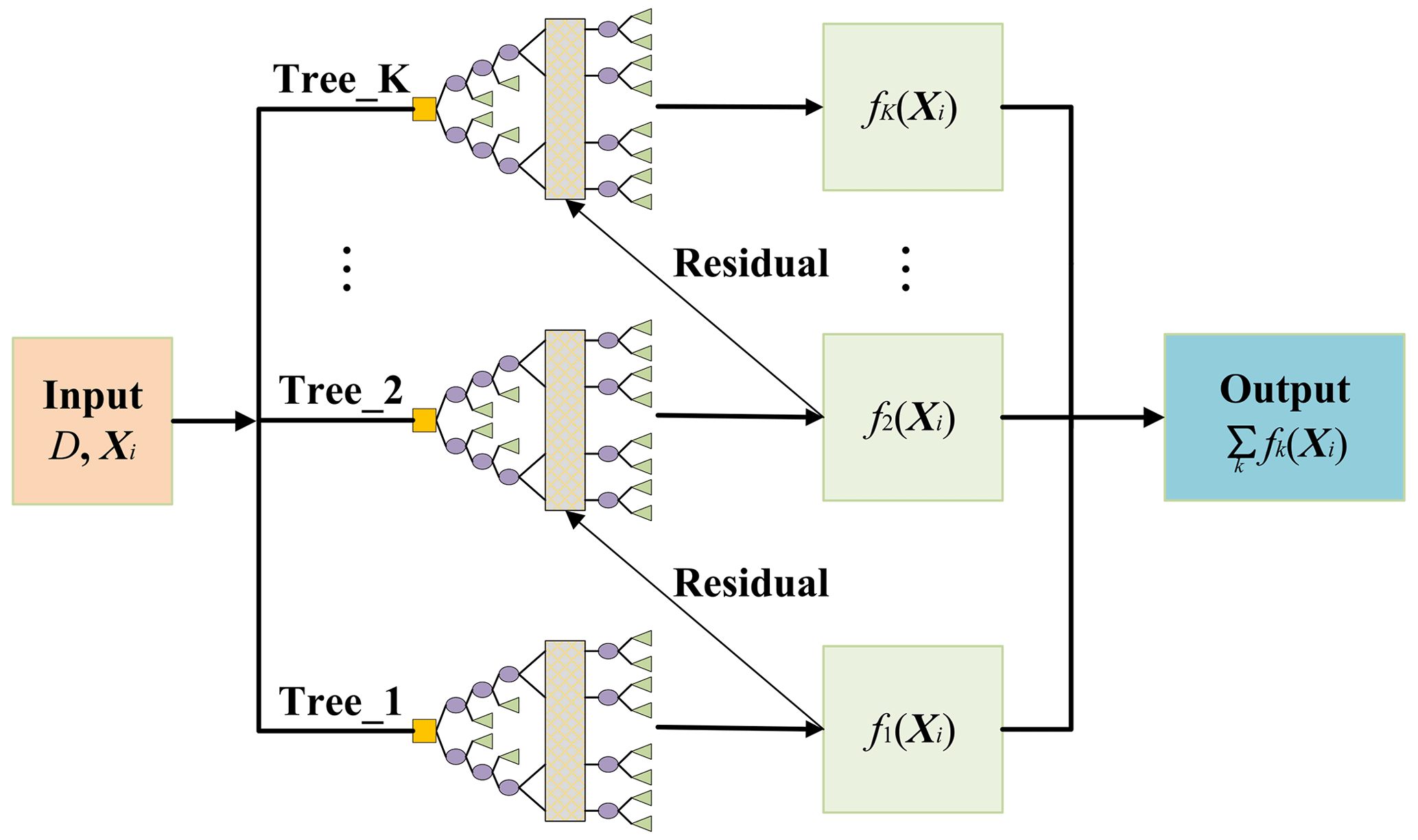
Figure 1 Flowchart of XGBoost for predicting ${\widehat{\mathit{r}}}_i$ based on a decision tree model. The yellow squares are the root nodes within each tree, which represent the input features in this paper. The purple ellipses denote the child nodes, where the model evaluates input features and makes decisions to split the data. The green rectangles depict the leaf nodes and refer to the prediction results. The vertical rectangles abstract the internal splitting processes of the trees, thus indicating decision-making not explicitly detailed in the diagram.

XGBoost trains G(X) in Eq. (5) by continuously fitting the residual error until the following objective function is minimized:

$$\begin{array}{}\text{(6)}& {\mathit{Obj}}^{\left(t\right)}=\sum _{i=\mathrm{1}}^n{\left({\mathit{r}}_i-\left({\widehat{\mathit{r}}}_i^{(t-\mathrm{1})}+f_t\left({\mathit{X}}_i\right)\right)\right)}^{\mathrm{2}}+\sum _{k=\mathrm{1}}^t\mathrm{\Omega }\left(f_k\right),\end{array}$$

where t represents the training of the tth tree and Ω(f_k) is the regularization term given by

$$\begin{array}{}\text{(7)}& \mathrm{\Omega }\left(f\right)=\mathrm{{\rm Y}}M+{\displaystyle \frac{\mathrm{1}}{\mathrm{2}}}\mathit{\lambda }\sum _{j=\mathrm{1}}^M{\mathit{\omega }}_j^{\mathrm{2}},\end{array}$$

where M is the number of leaf nodes, ω_j is the leaf node weight for the jth leaf node, and Υ and λ are penalty coefficients. The minimization of Eq. (6) provides a parametric model G(X) that maps the feature ensemble X extracted from μ_p to the source location r.

Table 1 Summary of basic information on the features of the observation series.

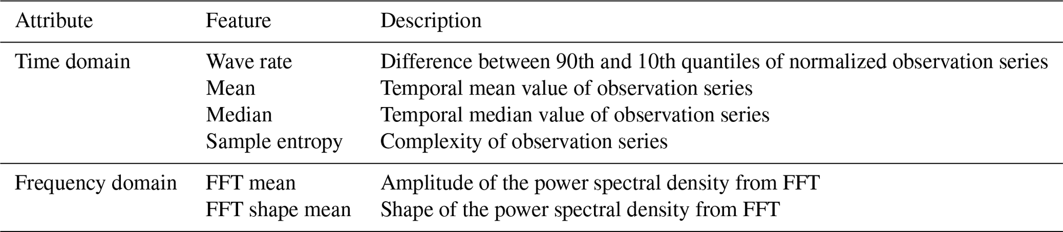
To comprehensively evaluate the influence of the source location, both time- and frequency-domain features (as outlined in Table 1) are considered during the training process and mapped to the source location by G(X). Among the time-domain features, the wave rate quantifies the fluctuations in μ_p over time, while the temporal mean and median values are measures of the central tendency of μ_p (Witte and Witte, 2017). The sample entropy measures the complexity of μ_p, with a lower sample entropy indicating greater self-similarity and less randomness in μ_p. The frequency-domain features are calculated based on the fast Fourier transform (FFT). The FFT mean is the mean value of the Fourier coefficients for μ_p, and the FFT shape mean describes the shape of the Fourier coefficients. These quantities are formulated as follows:

$$\begin{array}{}\text{(8)}& {\displaystyle }& {\displaystyle }\text{FFT\hspace{0.17em}\hspace{0.17em}mean}={\displaystyle \frac{\mathrm{1}}{N}}\sum _{k=\mathrm{1}}^N\left|{\mathit{\mu }}_{ik}\right|,\text{(9)}& {\displaystyle }& {\displaystyle }\text{FFT\hspace{0.17em}\hspace{0.17em}shape\hspace{0.17em}\hspace{0.17em}mean}={\displaystyle \frac{\mathrm{1}}{\sum _{k=\mathrm{1}}^N\left|{\mathit{\mu }}_{ik}\right|}}\sum _{k=\mathrm{1}}^{N}k\left|{\mathit{\mu }}_{ik}\right|,\end{array}$$

where μ_ik is the Fourier coefficient and N is the length of μ_p. These features are calculated from the simulated observations at each site and provided to XGBoost as initial inputs.

2.4 Release rate estimation

Once the source location has been retrieved, many existing methods can be used to inversely estimate the release rate. In this study, we choose the recently developed PAMILT method (Fang et al., 2022) because it can correct the intrinsic model errors of the release rate estimation and accurately retrieve the temporal variations in the release rates.

2.5 Numerical implementation

2.5.1 Pre-screening of potential source locations

To reduce the computational cost and remove low-quality samples, the search range for the source location is pre-screened by evaluating the correlation coefficients between the observations and atmospheric dispersion model simulations, with the candidate source locations randomly sampled in the considered calculation domain. Because the release rate is unknown, it is assumed to be 1 for all simulations. Source locations corresponding to the highest 40 % of correlation coefficients are selected as the search range of the subsequent refined source-location estimation using XGBoost.

2.5.2 Samples for training XGBoost

The samples for training G(X) in Eq. (5) are generated based on the simulations described in Sect. 2.5.1, and the source locations of these simulations are within the search range determined according to Sect. 2.5.1. The simulation data are scaled by a constant factor (the ratio between the median value of all observations and that of the simulations using a unit release rate), which ensures that the simulations and observations have the same order of magnitude. Gaussian noise is added to the simulation data to simulate the statistical fluctuations in the measurements. The simulations between the first and last data points above the noise level are filtered by a temporal sliding-window average filter with a window size of 5, yielding samples for feature extraction as described in Sect. 2.3.

2.5.3 Automatic optimization of the XGBoost model

The XGBoost model for source-location estimation is automatically optimized with respect to the hyperparameters and feature selection. Specifically, the Bayesian optimization algorithm is used to optimize the hyperparameters by minimizing the following generalization coefficient (GC) defined under the 5-fold cross-validation framework:

$$\begin{array}{}\text{(10)}& {\displaystyle }& {\displaystyle }\mathrm{GC}=(\mathrm{1}-\mathrm{MCV}{)}^{\mathrm{2}}+\text{Var}\left(R_k^{\mathrm{2}}\right),\text{(11)}& {\displaystyle }& {\displaystyle }\mathrm{MCV}={\displaystyle \frac{\mathrm{1}}{\mathrm{5}}}\sum _k{R}_k^{\mathrm{2}},\end{array}$$

where $R_k^{\mathrm{2}}$ is the goodness of fit and k is the index of each fold $(k=\mathrm{1},\mathrm{2},\mathrm{\dots },\mathrm{5})$. MCV is the mean cross-validation score $R_k^{\mathrm{2}}$ among the 5 folds, and $\text{Var}(R_k^{\mathrm{2}}$) measures the variance of $R_k^{\mathrm{2}}$. This function aims to balance the average and the variance of $R_k^{\mathrm{2}}$, thus enhancing the generalization ability of the XGBoost model. In this study, the optimized hyperparameters include max_depth (the maximum depth of a decision tree), learning_rate (the step size shrinkage when updating), n_estimators (the number of decision trees), min_child_weight (the minimum sum of sample weights of a child node), subsample (the subsample ratio of the training samples), colsample_bytree (the subsample ratio of the columns when constructing a decision tree), reg_lambda (the L2 regularization term based on weights), and gamma (the minimum loss reduction required to split the decision tree).

The initial input features (Table 1) are optimized through a feature selection step, where MCV serves as the selection criterion. The selection is implemented by recursively removing the feature with the least importance and reassessing the MCV based on cross-validation (Akhtar et al., 2020). Initially, an XGBoost model is trained with all features, and the importance of each feature is assessed based on its contribution to the model accuracy. The feature with the least importance is removed and the XGBoost model is retrained using the remaining features. The feature importance and MCV are updated accordingly, and another feature is removed. This iterative process continues until the optimal number of features is identified, which corresponds to the highest MCV achieved during the process. The overall flowchart of the proposed spatiotemporally separated source reconstruction model is shown in Fig. S1 in the Supplement.

2.6 Validation case

2.6.1 Field experiments

The proposed methodology was validated against the observations of the SCK CEN ⁴¹Ar and ETEX-1 field experiments. The SCK CEN ⁴¹Ar experiment was carried out at the Belgian Reactor 1 (BR1) research reactor in Mol, Belgium, in October 2001 as a collaboration between Nordic Nuclear Safety Research (NKS) and the Belgian Nuclear Research Centre (SCK CEN) (Rojas-Palma et al., 2004). The major part of the experiment was conducted on 3–4 October, during which time ⁴¹Ar was emitted from a 60 m stack with a release rate of approximately 1.5 × 10¹¹ Bq h⁻¹. Meteorological data such as wind speed and direction were provided by the on-site weather mast. For most of the experimental period, the atmospheric stability was neutral, and the wind was blowing from the southwest. As illustrated in Fig. 2a, the source coordinates were (650 m, 210 m). The 60 s average ground-level fluence rates were continuously collected by an array of NaI(Tl) gamma detectors, with different observation sites used on the 2 d. To convert the measured fluence rates to gamma dose rates (mSv h⁻¹), we used the ⁴¹Ar parameters from a previous study (Li et al., 2019a): E_γ = 1.2938 MeV, fⁿ(E_γ) = 0.9921, μ_a = 2.05 × 10⁻³ m⁻¹, and ω = 7.3516 × 10⁻¹ Sv Gy⁻¹. More details about these measurements can be found in Rojas-Palma et al. (2004).

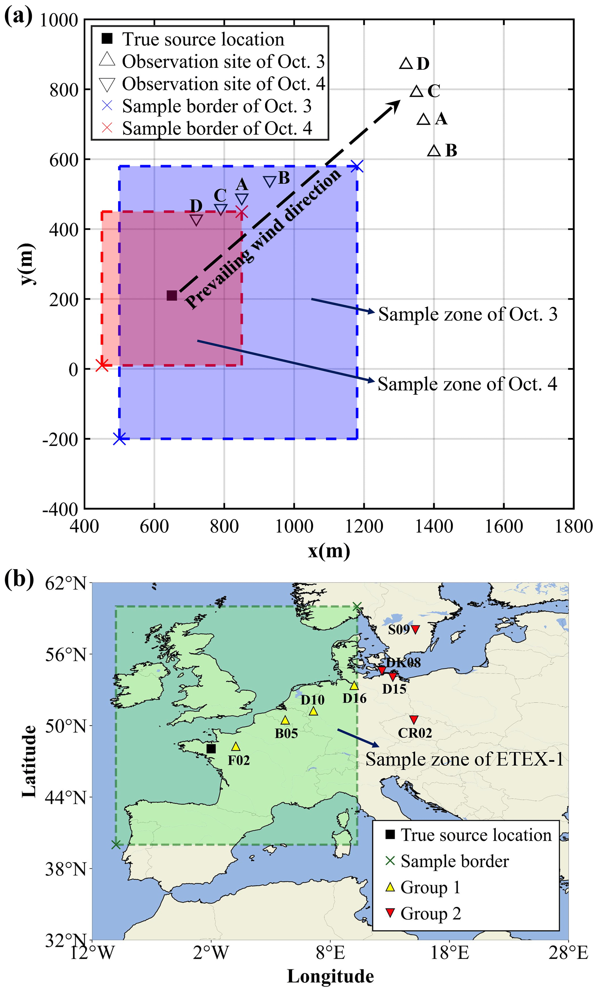
Figure 2 Release locations and observation sites in two field experiments. (a) The SCK CEN ⁴¹Ar experiment. The map was created based on the relative positions of the release source and the observation sites (Drews et al., 2002). The coordinates of the sample border were (500 m, −200 m) and (1180 m, 580 m) on 3 October and (450 m, 10 m) and (850 m, 450 m) on 4 October. This figure was plotted using MATLAB 2016b rather than a map provider. (b) The ETEX-1 experiment. The map was created based on the real longitudes and latitudes of the release source and the observation sites (Nodop et al., 1998). The coordinates of the sample border are (40° N, 10° W) and (60° N, 10° E). This figure was plotted using the cartopy function of Python rather than a map provider.

The ETEX-1 experiment took place at Monterfil in Brittany, France, starting on 23 October 1994 (Nodop et al., 1998). During ETEX-1, a total of 340 kg of PMCH was released into the atmosphere on 23 October 1994 at 16:00:00 UTC and 24 October 1994 at 03:50:00 UTC. As illustrated in Fig. 2b, the source coordinates were (48.058° N, 2.0083° W). A total of 3104 available observations (3 h averaged concentrations) were collected at 168 ground sites. ETEX-1 has been widely used as a validation scenario when reconstructing atmospheric radionuclide releases (Ulimoen and Klein, 2023; Tomas et al., 2021). The candidate source locations are uniformly sampled from the green-shaded zone. We choose two groups of observation sites: the first group comprises four sites (i.e., B05, D10, D16, and F02) randomly selected from the sites within the sample zone (Group 1, with a total of 92 available observations), and the second group involves four sites (i.e., CR02, D15, DK08, and S09) randomly selected from the sites beyond the sample zone boundaries (Group 2, with a total of 90 available observations). Compared with the SCK CEN ⁴¹Ar experiment, the ETEX-1 observations exhibit temporal sparsity, lower temporal resolution, and increased complexity of meteorological conditions.

2.6.2 Simulation settings of the atmospheric dispersion model

For the SCK CEN ⁴¹Ar field experiment, the Risø Mesoscale PUFF (RIMPUFF) model was employed to simulate the dispersion of radionuclides and calculate the dose rates at each observation site (Thykier-Nielsen et al., 1999). The simulations used meteorological data measured on-site and the modified Karlsruhe–Jülich diffusion coefficients. The calculation domain measured 1800 m × 1800 m, and the grid resolution was 10 m × 10 m. The release height of ⁴¹Ar was assumed to be 60 m. Other RIMPUFF calculation settings followed those of a previous study (Li et al., 2019a) and have been validated against the observations. To establish the datasets for the XGBoost model, 2050 simulations and 1000 simulations with different source locations were performed by RIMPUFF for the experiments on 3 and 4 October, respectively. Candidate source locations were randomly sampled from the shaded zones in Fig. 2a, which were determined according to the positions of the observation sites and the upwind direction. Each simulation, along with its corresponding source location, forms one sample. As described in Sect. 2.5.1, we calculated the correlation coefficient for each sample and preserved the 40 % of samples with the highest 40 % of correlation coefficients (i.e., 820 samples for 3 October and 400 samples for 4 October). The constant factors mentioned in Sect. 2.5.2 are 1.53 × 10¹¹ and 1.48 × 10¹¹ for 3 and 4 October, respectively.

For the ETEX-1 experiment, the FLEXible PARTicle (FLEXPART) model (version 10.4) was applied to simulate the dispersion of PMCH (Pisso et al., 2019). The meteorological data were obtained from the United States National Centers for Environmental Prediction Climate Forecast System Reanalysis and have a spatial resolution of 0.5° × 0.5° and a time resolution of 6 h. To rapidly establish the relationship between the varying source locations and the observations, 182 backward simulations were performed using FLEXPART with a time interval of 3 h, a grid size of 0.25° × 0.25°, and eight vertical levels (from 100–50 000 m). Only the lowest model output layer was used for source reconstruction. Candidate source locations were uniformly sampled from the shaded zone in Fig. 2b, resulting in a total of 6561 source locations. As described in Sect. 2.5.1, 2624 candidate source locations were preserved following the pre-screening step. The constant factors mentioned in Sect. 2.5.2 are 5.60 × 10¹² and 2.86 × 10¹³ for Group 1 and Group 2, respectively.

2.7 Sensitivity study

1. Search range. The search range is controlled by the pre-screening threshold, which is the top proportion of the correlation coefficients in the pre-screening step. Specifically, we use source locations corresponding to the highest 20 %, 40 %, 50 %, 60 %, 80 %, and 100 % of correlation coefficients to define the search ranges, with a lower proportion indicating a narrower and more focused search area.

2. Size of the sliding window. Temporal filtering with different sliding-window sizes is applied to separate the source-location estimation from the release rate estimation. In this study, the size of the sliding window ranges from 3–10. With these filtered data, the XGBoost model is trained using the same pattern for the source-location estimation.

3. Feature type. The XGBoost model is trained using only time-domain features and only frequency-domain features to investigate the influence of these features on the source-location estimation. The performance of the time-feature-only and frequency-feature-only models is compared with the all-features result.

4. Number and combination of observation sites. The XGBoost model is trained and applied to the source-location estimation with different numbers of observation sites, namely a single site, two sites, and three sites. For the two- and three-site cases, the model is trained using different combinations of sites and the source location is estimated accordingly.

5. Meteorological errors. Meteorological errors, especially the random errors in the wind field (Mekhaimr and Abdel Wahab, 2019), are important uncertainties in source reconstruction. To simulate such uncertainties, a stochastic perturbation of ± 10 % is introduced into the x and y components of the observed wind speeds, and a perturbation of ± 1 stability class is applied to the stability parameters (e.g., from C to B or D). For both days, 50 meteorological groups are generated based on these random perturbations.

In all the sensitivity tests, the source location is estimated 50 times with randomly initialized hyperparameters to demonstrate the uncertainty range of the proposed method under different circumstances. The performance of source-location estimation is compared quantitatively using the metrics specified in Sect. 2.8.3.

2.8 Performance evaluation

2.8.1 Observation filtering

The feasibility of filtering is demonstrated using both the synthetic and the real observations of the SCK CEN ⁴¹Ar experiment and the real observations of the ETEX-1 experiment. The synthetic observations are generated by a simulation using a synthetic temporally varying release profile with sharply increasing, stable, and gradually decreasing phases (as illustrated in Fig. S2), which is typical of an atmospheric radionuclide release (Davoine and Bocquet, 2007). Because several temporal observations are missing at some observation sites, we only choose observations sampled between 09:00:00 UTC on 24 October 1994 and 03:00:00 UTC on 26 October 1994 for the source-location estimation. The simulations corresponding to the synthetic and real observations should first be processed following the procedure described in Sect. 2.5.2. The filtering performance is evaluated by comparing the simulation–observation differences before and after the filtering step. Several statistical metrics can be used to quantify this difference, including the normalized mean square error (NMSE), Pearson's correlation coefficient (PCC), and the fraction of predictions within a factor of 2 or a factor of 5 of the observations (FAC2 or FAC5, respectively) (Chang and Hanna, 2004).

2.8.2 Optimization of the XGBoost model

The hyperparameters are optimized with respect to the GC in Eq. (10), and the features are optimized with respect to the MCV in Eq. (11). Larger values of MCV and smaller values of GC indicate better optimization performance. In addition, the importance of each feature to the XGBoost training is evaluated with the built-in feature importance measure of the XGBoost model.

Table 2 Parameter settings of the field experiments.

2.8.3 Source reconstruction

The relative errors in the source location (δ_r) and total release (δ_Q) are calculated to evaluate the source reconstruction accuracy:

$$\begin{array}{}\text{(12)}& {\displaystyle }& {\displaystyle }{\mathit{\delta }}_{\mathit{r}}={\displaystyle \frac{\left|{\mathit{r}}_{\text{true}}-{\mathit{r}}_{\text{est}}\right|}{L_{\mathrm{D}}}}\times \mathrm{100}\mathit{\%},\text{(13)}& {\displaystyle }& {\displaystyle }{\mathit{\delta }}_Q={\displaystyle \frac{Q_{\text{true}}-Q_{\text{est}}}{Q_{\text{true}}}}\times \mathrm{100}\mathit{\%},\end{array}$$

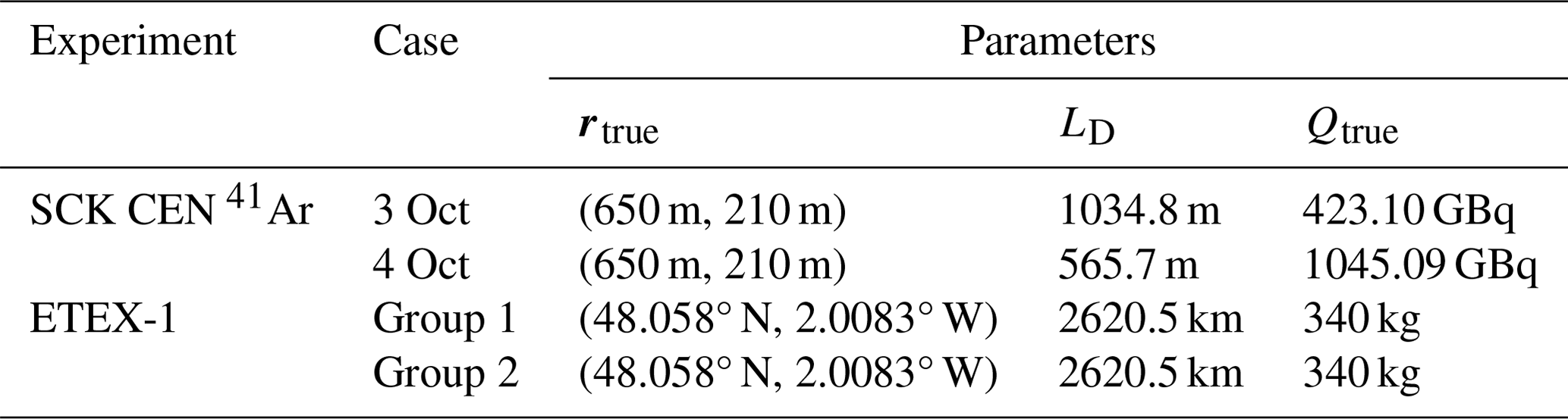
where r_true and Q_true refer to the real source location and total release in the field experiment, respectively, and r_est and Q_est are the estimated location and total release, respectively. L_D represents the range of the source domain, which is the distance between the lower and upper borders of the sampled zone (Fig. 2). The values of r_true, L_D, and Q_true are listed in Table 2. In addition to the total release, the reconstructed release rates are also compared with the true temporal release profile.

2.8.4 Comparison with the Bayesian method

The proposed method is compared with the popular Bayesian method based on the SCK CEN ⁴¹Ar and ETEX-1 experiments, with the same search range used for locating the source in both methods (Fig. 2). The Bayesian method is augmented with an in-loop inversion of the release rate at each iteration of the Markov chain Monte Carlo sampling. The prior distribution of the Bayesian method is a uniform distribution, and the likelihood is a log-Cauchy distribution. More detailed information is presented in Note S1 in the Supplement.

2.8.5 Uncertainty range

The uncertainty ranges are calculated and compared for the correlation-based method, the Bayesian method, and the proposed method. For the correlation-based method, the uncertainty range is calculated using the source locations with the top 50 correlation coefficients. For the proposed method, the uncertainty range is calculated from 50 Monte Carlo runs with randomly initialized hyperparameters. The Bayesian method provides the uncertainty range directly through the posterior distribution. For consistency with the other two methods, the results with the top 50 frequencies are selected for the comparison.

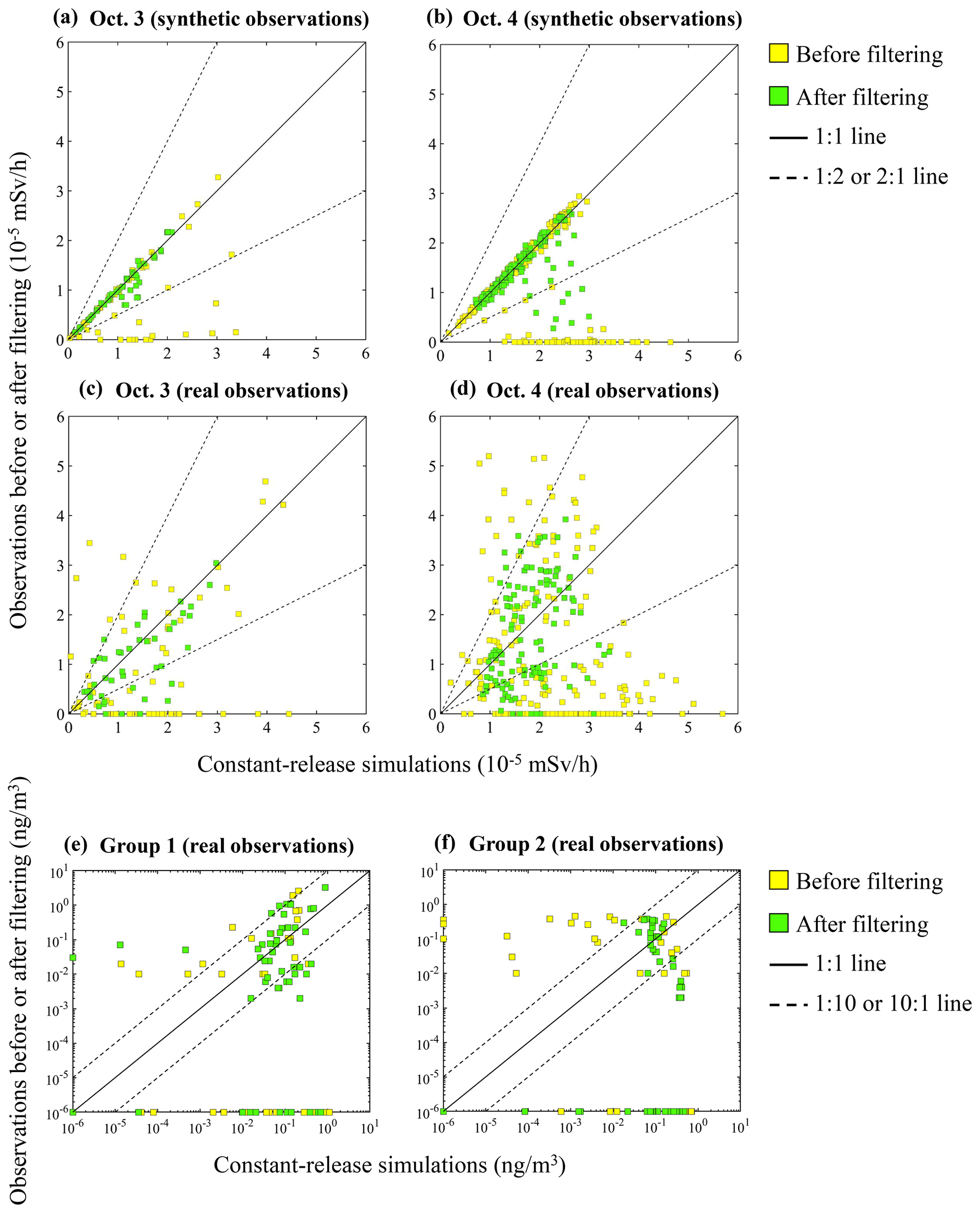
Figure 3 Scatterplots of the original (yellow squares) and filtered (green squares) observations versus the constant-release simulation results. SCK CEN ⁴¹Ar experiment: (a) 3 October (synthetic observations); (b) 4 October (synthetic observations); (c) 3 October (real observations); (d) 4 October (real observations). ETEX-1 experiment: (e) Group 1 (real observations); (f) Group 2 (real observations).

3 Results and discussion

3.1 Filtering performance

Figure S3 displays the original and filtered observations at different observation sites for both days. The results demonstrate that the peak values have been smoothed out and the long-term trends are preserved to a large degree. Figure 3 compares the filtering performance for the synthetic and real observations, where the constant-release simulations are plotted against the observations before and after filtering. For the synthetic observations, the filtered data are more concentrated along the 1:1 line for both days, and all filtered data fall within the 2-fold lines for 3 October. For the real observations, the dots before filtering in Fig. 3 have a dispersed distribution for both 3 and 4 October, indicating limited correlations with the simulations. After filtering, the dots are more concentrated towards the 1:1 line for both the SCK CEN ⁴¹Ar and the ETEX-1 experiments. These phenomena indicate a noticeably increased agreement between the filtered observations and the constant-release simulations.

Table 3 Quantitative metrics for the filtering validation.

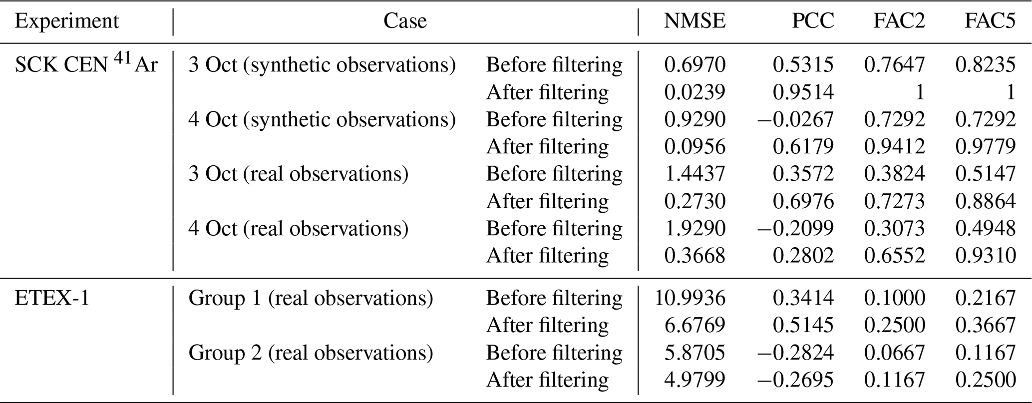
Table 3 quantitatively compares the results presented in Fig. 3. For each case, all metrics are greatly improved after filtering, confirming the better agreement between the filtered observations and the constant-release simulations. The improved agreement indicates that the filtering step significantly reduces the influence of temporal variations in release rates across the observations. The filtering performs better with the synthetic observations than with the real observations because the synthetic observations are free of measurement errors. The filtering process produces a better effect with the SCK CEN ⁴¹Ar experiment than with the ETEX-1 experiment, owing to the sparser observations in the ETEX-1 experiment (Fig. S3).

3.2 Optimization of the XGBoost model

3.2.1 Hyperparameters

Table S1 in the Supplement summarizes the optimal hyperparameters and corresponding GCs used for source-location estimation in this study; Tables S2–S5 include all the optimal hyperparameters used in the 50 runs of the SCK CEN ⁴¹Ar and ETEX-1 experiments. The optimal GCs of the SCK CEN ⁴¹Ar experiment are smaller than those of the ETEX-1 experiment, indicating better fitting performance. This is because the sparse observations of the ETEX-1 experiment (Fig. S3) are more sensitive to the added Gaussian noise (see Sect. 2.5.2).

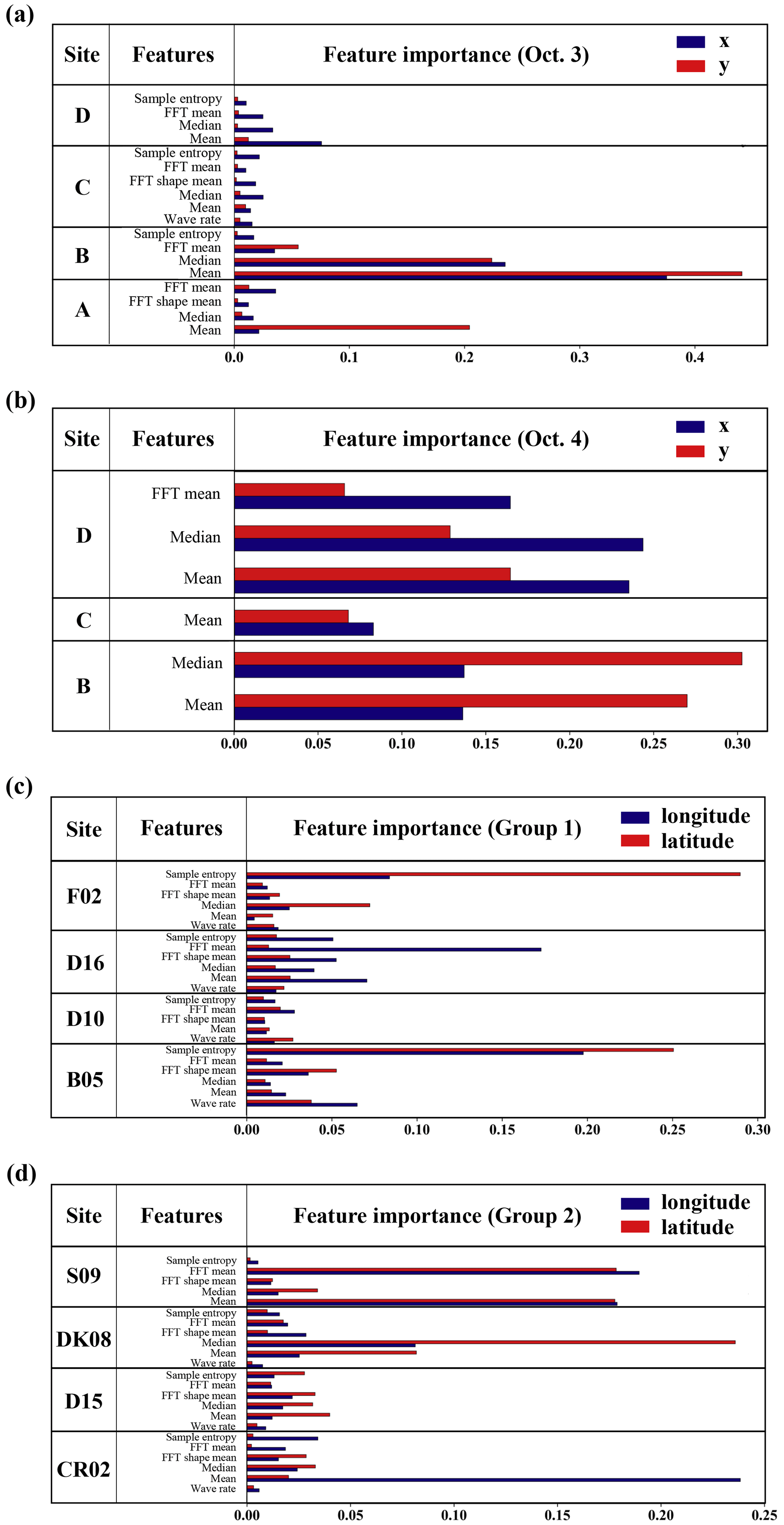
Figure 4 Feature importance. SCK CEN ⁴¹Ar experiment: (a) 3 October; (b) 4 October. ETEX-1 experiment: (c) Group 1; (d) Group 2.

3.2.2 Feature selection

Figure 4 compares the importance of the selected features at each site for the two experiments. The time-domain features are dominant for both days in the SCK CEN ⁴¹Ar experiment (Fig. 4a and b). For 3 October, Site B is the most important, possibly because it is farthest away in the crosswind direction. For 4 October, the four sites provide redundant feature information, and many features are removed. This is because the distribution of observation sites is almost parallel to the wind direction on this day. According to Fig. S3b, the measurements from Sites A and B have a high correlation, thus leading to the removal of features from Site A on 4 October. In summary, the feature selection process adapts XGBoost to different application scenarios. Figure S4a and b show the variations in MCV with the number of features for the x and y coordinates. The MCV first increases with the number of features and then decreases slightly after reaching the maximum. The optimal number of features for 4 October is noticeably smaller than for 3 October. In addition, the selected features for 3 October involve all four sites, whereas those for 4 October involve three sites. The reduced features and site numbers indicate a high level of redundancy in the observations acquired on 4 October. This is because the observation sites are parallel to the downwind direction and provide similar location information in the crosswind direction.

For the ETEX-1 experiment, Fig. 4c and d show that the features of Group 1 and Group 2 are largely preserved after the feature selection process (only one feature is removed for each case), indicating less redundancy than that in the SCK CEN ⁴¹Ar experiment. The time-domain features are dominant, but the frequency-domain features at some sites (e.g., D16 and S09) also play important roles. The MCVs of the ETEX-1 experiment have similar variation trends to those for the SCK CEN ⁴¹Ar experiment (Fig. S4c and d).

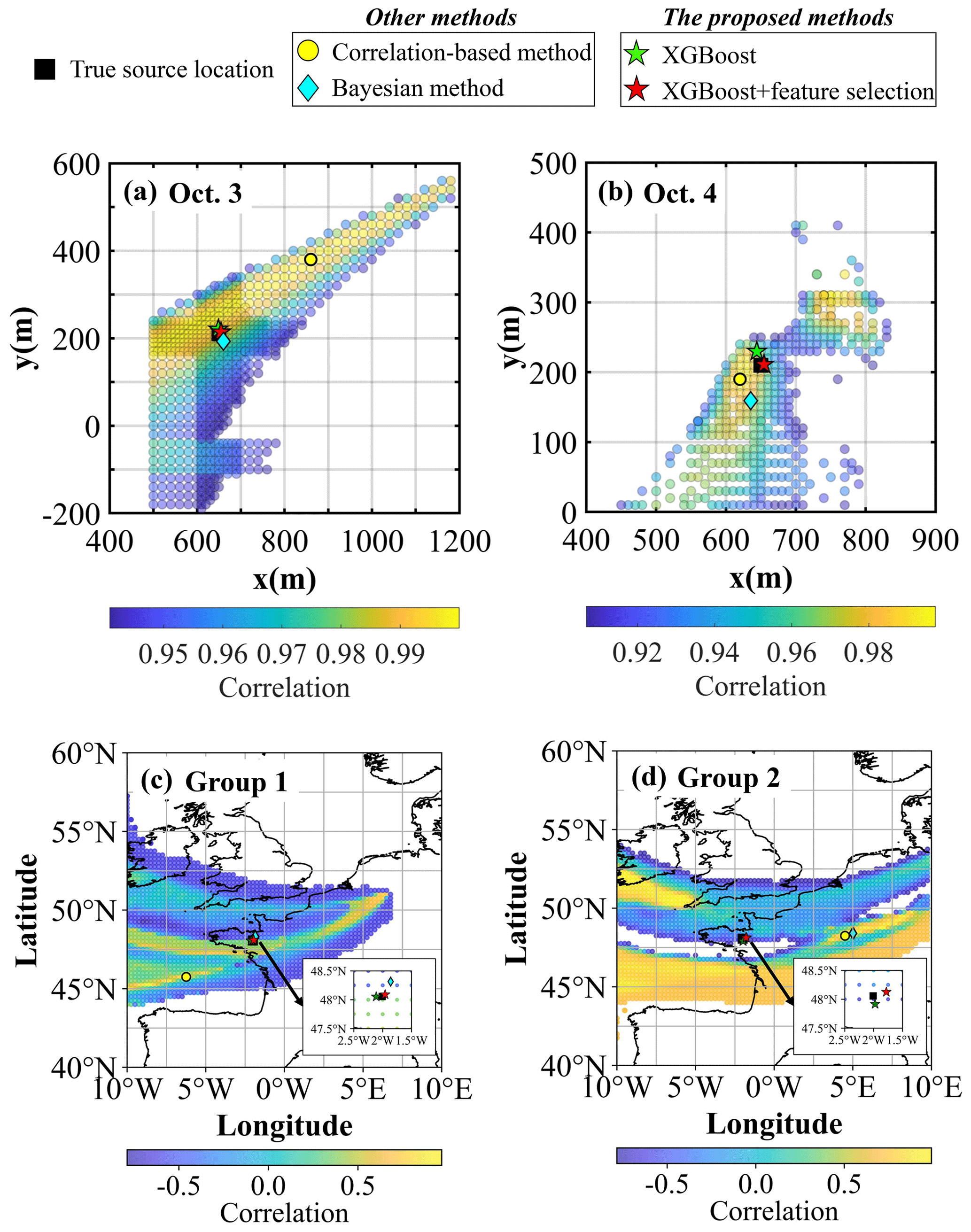
Figure 5 Source-location estimation results. SCK CEN ⁴¹Ar experiment: (a) 3 October; (b) 4 October. ETEX-1 experiment: (c) Group 1; (d) Group 2. A detailed enlargement of the region from (47.5° N, 2.5° W) to (48.5° N, 1.5° W) is shown in the bottom-right corner in (c) and (d) to highlight the source-location estimation results of the proposed method. The yellow dots denote the maximum-correlation points, which are the results of the correlation-based method. The green and red stars represent the results based on XGBoost before and after feature selection, respectively. The cyan diamonds represent the results based on the Bayesian method.

3.3 Source reconstruction

3.3.1 Source locations

Figure 5 compares the best-estimated source locations of the correlation-based method, the Bayesian method, and the proposed method with the ground truth. The pre-screening zone covers the true source location for both days, but the areas with the highest correlation coefficients are still too large for the point source to be accurately located. The locations with the maximum correlation exhibit errors of 270.19 and 36.06 m for 3 and 4 October, respectively, indicating that the correlation-based method may produce biased results in the case of non-constant releases. The Bayesian method estimates the location with errors of 19.62 and 52.81 m for 3 and 4 October, respectively. In comparison, the proposed method achieves the best performance. The estimates without feature selection are only 10.65 m (3 October) and 20.62 m (4 October) away from the true locations. Feature selection further reduces these errors to 6.19 m (3 October; a relative error of 0.60 %) and 4.52 m (4 October; a relative error of 0.80 %), which are below the grid size (10 m × 10 m) of the atmospheric dispersion simulation. The ability to estimate the source location with an accuracy surpassing the grid size can be attributed to the strong fitting capability of the optimized XGBoost model (Chen and Guestrin, 2016; Grinsztajn et al., 2022). However, this capability, although inherent, is not present across all optimized XGBoost models, as external factors such as observation noise and meteorological data inaccuracies can also impact the accuracy of source-location estimation.

For the ETEX-1 experiment, the pre-screening zone also covers the true source location for Group 1 and Group 2. The source locations estimated by the correlation-based method are 411.85 and 486.41 km away from the ground truth for Group 1 and Group 2, respectively. The location error in the Bayesian method estimates is only 30.50 km for Group 1 but increases to 520.77 km for Group 2, indicating the sensitivity of this method to the observations. In contrast, the proposed method achieves much lower source-location errors of 5.19 km for Group 1 (a relative error of 0.20 %) and 17.65 km for Group 2 (a relative error of 0.70 %). Group 1 exhibits a lower source-location error than Group 2 because the observation sites of Group 1 are closer to the sampled source locations than those of Group 2 and better characterize the plume. Feature selection did not remove many features (Fig. 4c and d), so the estimated source locations with and without feature selection basically overlap for both groups.

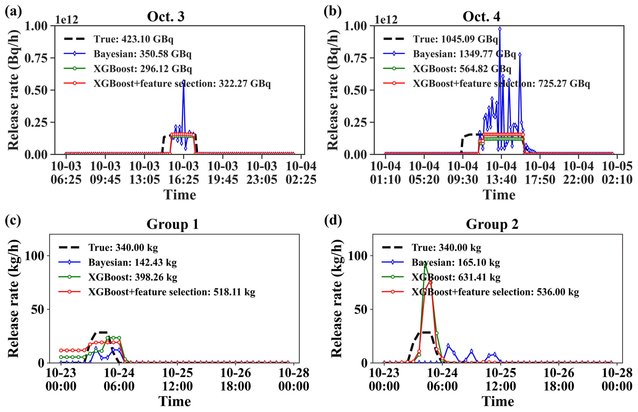
Figure 6 Release rate estimation results with different location estimates. SCK CEN ⁴¹Ar experiment: (a) 3 October; (b) 4 October. ETEX-1 experiment: (c) Group 1; (d) Group 2. The release rates labeled “XGBoost” or “XGBoost+feature selection” were estimated using the PAMILT method.

3.3.2 Release rates

Figure 6 displays the release rates estimated by the Bayesian and PAMILT methods based on the source location estimates in Fig. 5. For the SCK CEN ⁴¹Ar experiment (Fig. 6a and b), the release rates provided by the Bayesian method present several sharp peaks, corresponding to overestimates of up to 269.03 % (3 October) and 532.35 % (4 October). Furthermore, the Bayesian estimates exhibit unrealistic oscillations in the stable release phase. In contrast, the PAMILT method successfully retrieves the peak releases without oscillations for both days. Both the Bayesian and PAMILT estimates give delayed release start times but accurately estimate the end times, especially for 3 October. The PAMILT estimate underestimates the total release by 30.01 % and 45.95 % for 3 and 4 October, respectively; these values decrease to about 23.83 % and 30.60 %, respectively, after feature selection. The Bayesian method gives better total releases because of the overestimated peaks.

For the ETEX-1 experiment (Fig. 6c and d), the Bayesian estimates exhibit notable fluctuations, leading to underestimations of 58.11 % for Group 1 and 51.44 % for Group 2. Furthermore, the temporal profile of the Bayesian estimates for Group 2 falls completely outside the true-release window. In contrast, most releases using the PAMILT estimates are within the true-release time window, especially for Group 2, despite the overestimations reaching 52.38 % for Group 1 and 57.65 % for Group 2, after the feature selection process. Compared with the SCK CEN ⁴¹Ar experiment, the increased deviation in the ETEX-1 experiment is caused by the sparsity of observations at the four sites (Fig. S3).

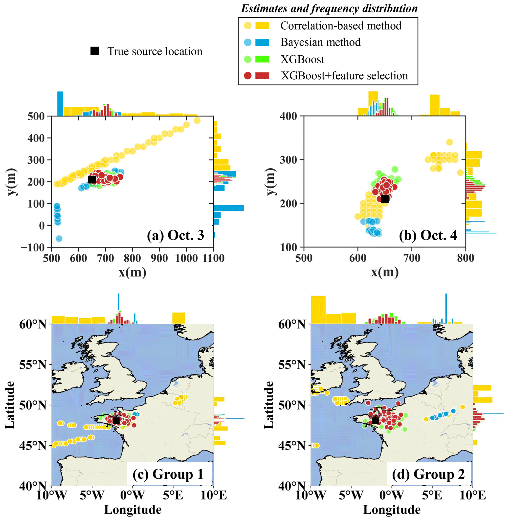
Figure 7 Spatial distributions of 50 source-location estimates. SCK CEN ⁴¹Ar experiment: (a) 3 October; (b) 4 October. ETEX-1 experiment: (c) Group 1; (d) Group 2. Each circle denotes an individual estimate as detailed in Sect. 2.8.5, with color variations indicating the respective method employed. Histograms along the axes represent the frequency distribution of the estimates along the respective axis.

3.3.3 Uncertainty range

Figure 7 compares the spatial distributions of 50 estimates produced by different methods. For the SCK CEN ⁴¹Ar experiment, the estimates of the correlation-based method are highly dispersed for both days, leading to a very uniform distribution of the x coordinate for 3 October and two separate distributions of both coordinates for 4 October. For both days, the Bayesian method produces a multimodal distribution in which the estimates are more concentrated than those of the correlation-based method. The corresponding full posterior distributions in Fig. S5a and b better reveal the multimodal feature of the Bayesian method, with several peaks of similar probabilities in the estimates of both coordinates on 3 October and the y coordinate on 4 October. The multimodal feature indicates the difficulty of constraining the solution in simultaneous spatiotemporal reconstruction, as reported in a previous study (De Meutter and Hoffman, 2020). In comparison, the proposed method provides the most concentrated source-location estimates. The feature selection moves the center of the distribution closer to the true location and narrows the distribution of the estimates, especially for 4 October.

For the ETEX-1 experiment, the estimates of the correlation-based method are quite dispersed, whereas those of the Bayesian method are more concentrated. The Bayesian estimates are close to the truth for Group 1 but deviate noticeably for Group 2. This phenomenon indicates that the Bayesian method is sensitive to the observations, especially when the observations are sparse. Figure S5c and d reveal that the Bayesian-estimated posterior distribution is multimodal for both ETEX-1 groups; this can be avoided by using additional observations (Fig. S5e). In contrast, the proposed method provides estimates that are concentrated around the truth for both Group 1 and Group 2, indicating its efficiency in the case of sparse observations. Due to the shorter distance between observation sites and the sampled source locations, the uncertainty range of the source location for Group 1 is narrower than that for Group 2.

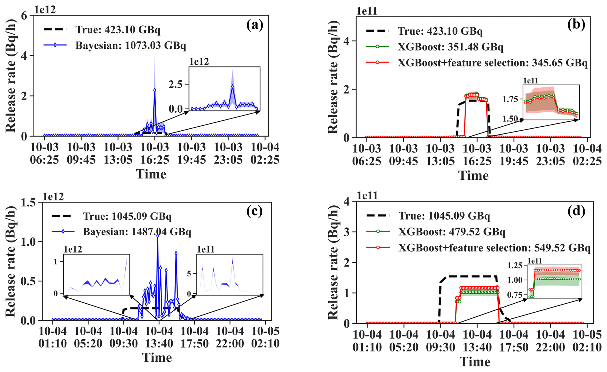
Figure 8 Release rate estimates over 50 calculations of the SCK CEN ⁴¹Ar experiment. (a) Estimates from the Bayesian method for 3 October. (b) Estimates from the PAMILT method for 3 October. (c) Estimates from the Bayesian method for 4 October. (d) Estimates from the PAMILT method for 4 October. The shading represents the uncertainty range between the lower quartile and the upper quartile. The shading in each figure is amplified in a subgraph. The legends in each figure provide the mean estimates for the total release.

Figure 8 compares the uncertainty ranges and mean total releases of the release rate estimations for the SCK CEN ⁴¹Ar experiment. For 3 October, the Bayesian estimates significantly overestimate the mean values and have a large uncertainty range, whereas the mean PAMILT estimate is very close to the true release and the uncertainty range is smaller than that from the Bayesian method. For 4 October, the mean Bayesian estimate exhibits greater deviations than the mean PAMILT estimate. Feature selection improves the mean estimate and reduces the uncertainty range of PAMILT because it improves the source-location estimation, thus reducing the deviation in the inverse model of the release rate. On 3 and 4 October, the PAMILT method underestimates the total release by 18.30 % and 47.42 %, respectively, whereas the Bayesian method gives overestimations of 153.61 % and 42.29 %, respectively.

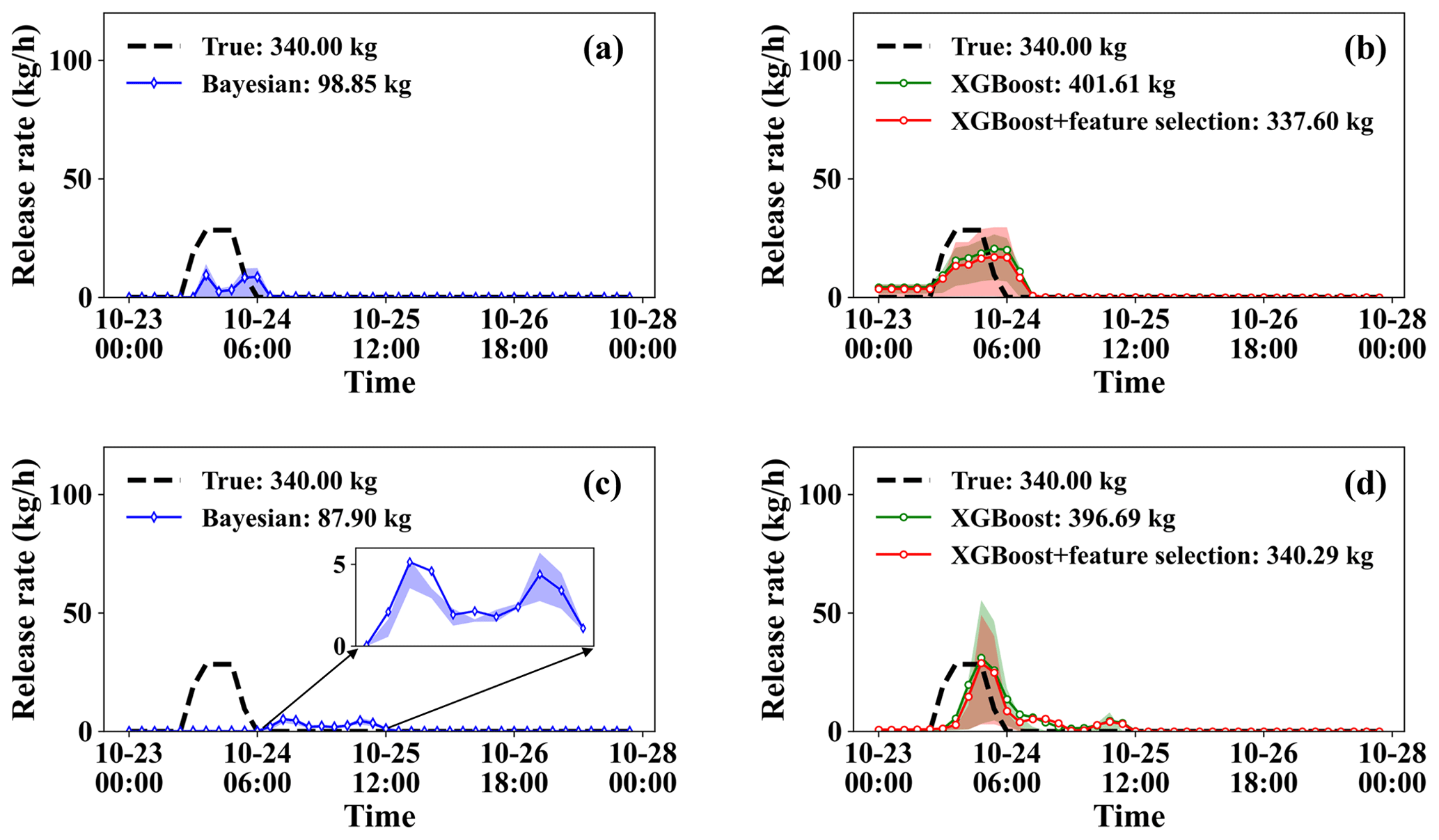
Figure 9 Release rate estimates over 50 calculations of the ETEX-1 experiment. (a) Estimates from the Bayesian method for Group 1. (b) Estimates from the PAMILT method for Group 1. (c) Estimates from the Bayesian method for Group 2. (d) Estimates from the PAMILT method for Group 2.

Figure 9 compares the uncertainty ranges of the release rate estimates for the two ETEX-1 groups. For both groups, the Bayesian estimates exhibit noticeable underestimations (including in the mean estimate) and small uncertainty ranges (Fig. 9a and c). The Bayesian estimates fall completely outside the true-release window for Group 2 (Fig. 9c). The mean PAMILT estimates are more accurate than the mean Bayesian estimates, with most releases occurring within the true-release window (Fig. 9b and d). However, the PAMILT estimates have a larger uncertainty range for the ETEX-I experiment than for the SCK CEN ⁴¹Ar experiment, implying that the source–receptor matrices of the ETEX-1 experiment are more sensitive to errors in source location than those of the SCK CEN ⁴¹Ar experiment are. This greater sensitivity originates from the complex meteorology in the ETEX-1 experiment. As with the mean total releases, the Bayesian method produces underestimations of 70.93 % for Group 1 and 74.15 % for Group 2. In comparison, the proposed method gives deviations of only 0.71 % for Group 1 and 0.09 % for Group 2 after feature selection.

Table 4 Relative errors in source reconstruction. δ_r represents the relative error in source location, which is positive, and δ_Q denotes the relative error in the total release, where a positive value indicates overestimation and a negative value denotes underestimation.

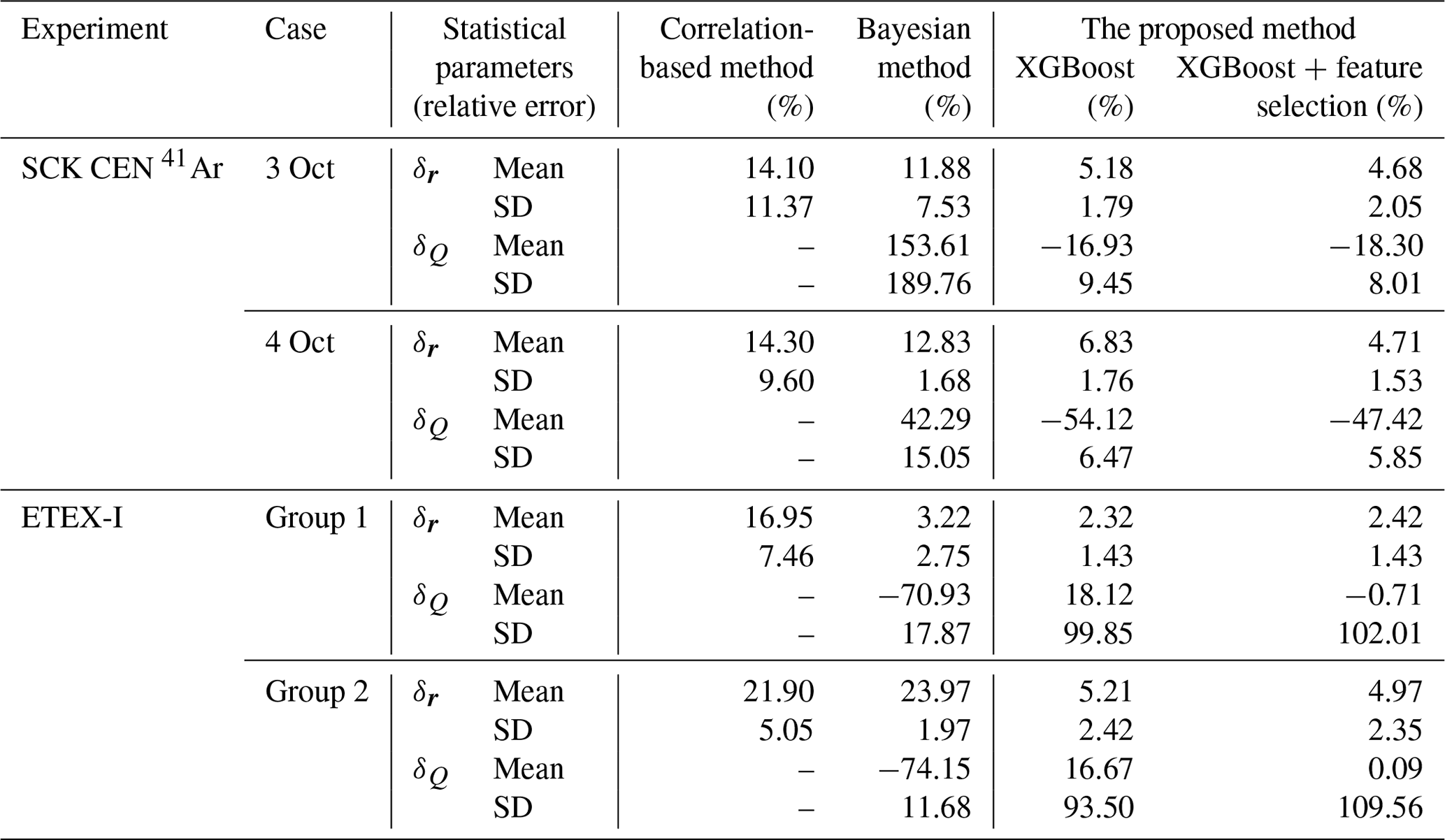
Table 4 lists the mean and standard deviation of the relative error for the 50 estimates given by different methods. The correlation-based method produces the largest mean relative error and standard deviation for source-location estimation, except for Group 2 of ETEX-I. For the SCK CEN ⁴¹Ar experiment, the proposed method gives the smallest mean error, about half of that of the Bayesian method. Its standard deviation is around one-quarter of that of the Bayesian method for 3 October but slightly larger for 4 October. For the total release, the PAMILT method gives a better standard deviation of the relative error for both days and a better mean relative error for 3 October, whereas the Bayesian method produces a better mean relative error for 4 October. Feature selection reduces the mean relative error, except for the total release for 3 October, and slightly increases the standard deviation of the source location and the total release results for 3 October. The mean relative error in the total release averaged over the 2 d is 65.09 % lower than that of the Bayesian method.

For the ETEX-1 experiment, the Bayesian method exhibits case-sensitive performance with respect to the mean relative error in source-location estimation, whereas the proposed method gives the most accurate source locations, with small uncertainties for both groups. As with the total release, the proposed method gives smaller mean relative errors than the Bayesian method, but the Bayesian method has a smaller standard deviation. Feature selection significantly reduces the mean relative error for the two groups. The mean relative error in the total release averaged over the two groups is 72.14 % lower than that of the Bayesian method.

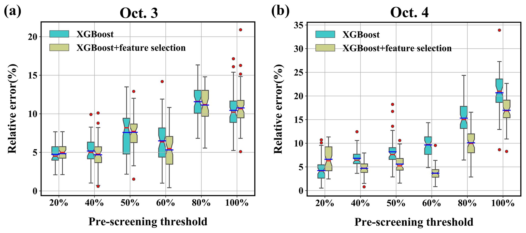
Figure 10 Distribution of the relative error (%) over 50 runs with different search ranges. The solid blue and solid red lines denote the average relative error (%) and median relative error (%), respectively. The upper and lower boundaries represent the upper and lower quartiles of the relative error (%), respectively. The fences are 1.5 times the interquartile ranges of the upper and lower quartiles. The red circles denote data that are not included between the fences. (a) 3 October; (b) 4 October.

3.4 Sensitivity analysis results

3.4.1 Sensitivity to the search range

Figure 10 displays the source-location errors obtained using different pre-screening thresholds to determine the search range. The error is smaller with a lower threshold, implying that a small search range helps reduce the mean and median errors. As the threshold increases, the mean and median errors, as well as the error range, show an overall tendency to increase but not in a strictly monotonic way. The mean and median errors are less than 12 % for 3 October and less than 22 % for 4 October, indicating robust performance in these tests. Feature selection reduces the mean, median, range, and lower bound of the errors in most tests, demonstrating its efficiency.

Figure 11 Sensitivity to the size of the sliding window. (a) 3 October; (b) 4 October.

3.4.2 Sensitivity to the size of the sliding window

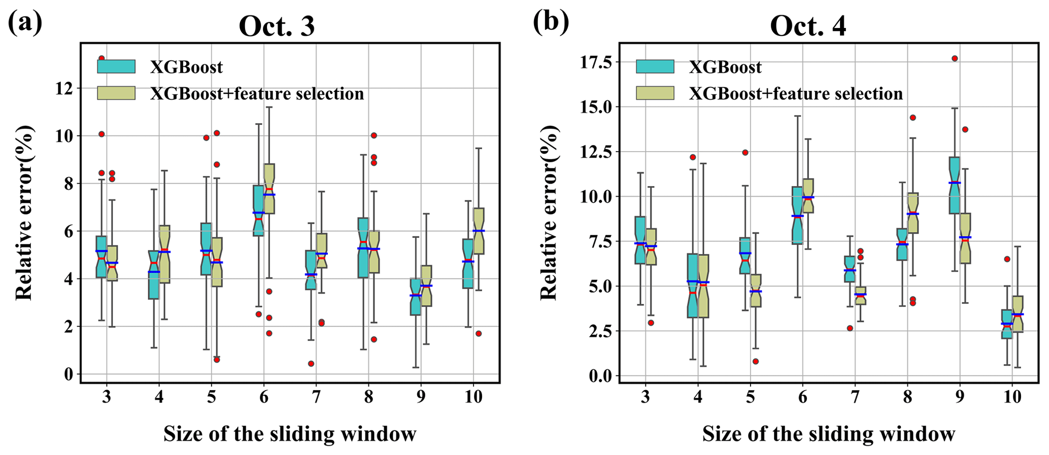
Figure 11 shows the source-location errors obtained with different sliding-window sizes. The mean and median errors are less than 8 % for 3 October and less than 11 % for 4 October, both of which are smaller than for the various search ranges. This indicates that the proposed method is more robust to this parameter than to the search range. For both days, the lowest mean, median, and error range occur with relatively large window sizes, i.e., a window size of 9 for 3 October and a window size of 10 for 4 October. This is because a large window size increases the strength of the filtering and removes the temporal variations in the release rates more completely. However, a large window size leads to an increased computational cost. Because the errors vary in a limited range, a medium window size provides a better balance between accuracy and computational cost. Feature selection improves the results for medium and small window sizes but may have less of an effect with large window sizes. This tendency implies that it is more appropriate to apply feature selection with medium window sizes than with large window sizes, as done in this study.

Figure 12 Sensitivity to the feature type. (a) 3 October; (b) 4 October.

3.4.3 Sensitivity to the feature type

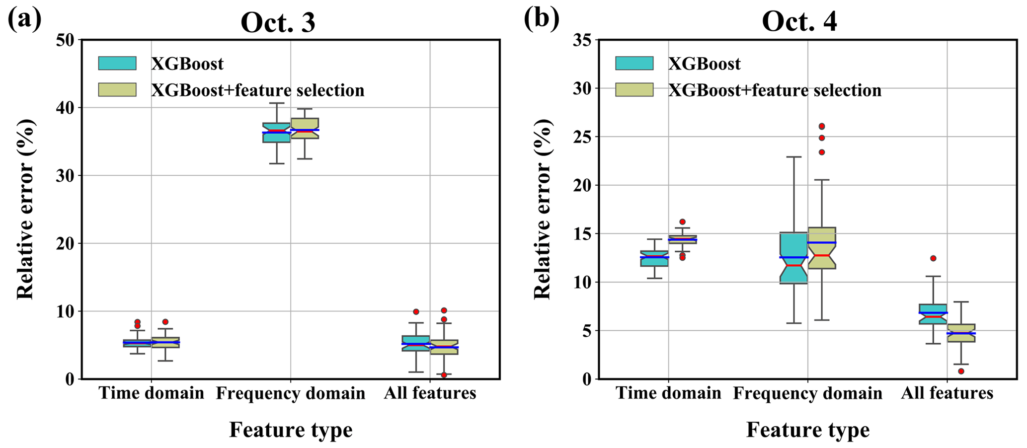
Figure 12 compares the results obtained with different feature types. For 3 October, the source-location errors are quite low when using only the time-domain features for the reconstruction; indeed, the errors are only slightly larger than when using all the features. In contrast, the results obtained using only the frequency-domain features exhibit larger errors, indicating that the time-domain features make a greater contribution to the results for 3 October. For 4 October, the mean source-location errors are similar when using either the time- or frequency-domain features, but the error range is higher when the frequency-domain features are used. In addition, the errors in both the single-domain-feature results are higher than those of the all-feature results, indicating that both feature types should be included to ensure accurate and robust source-location estimation.

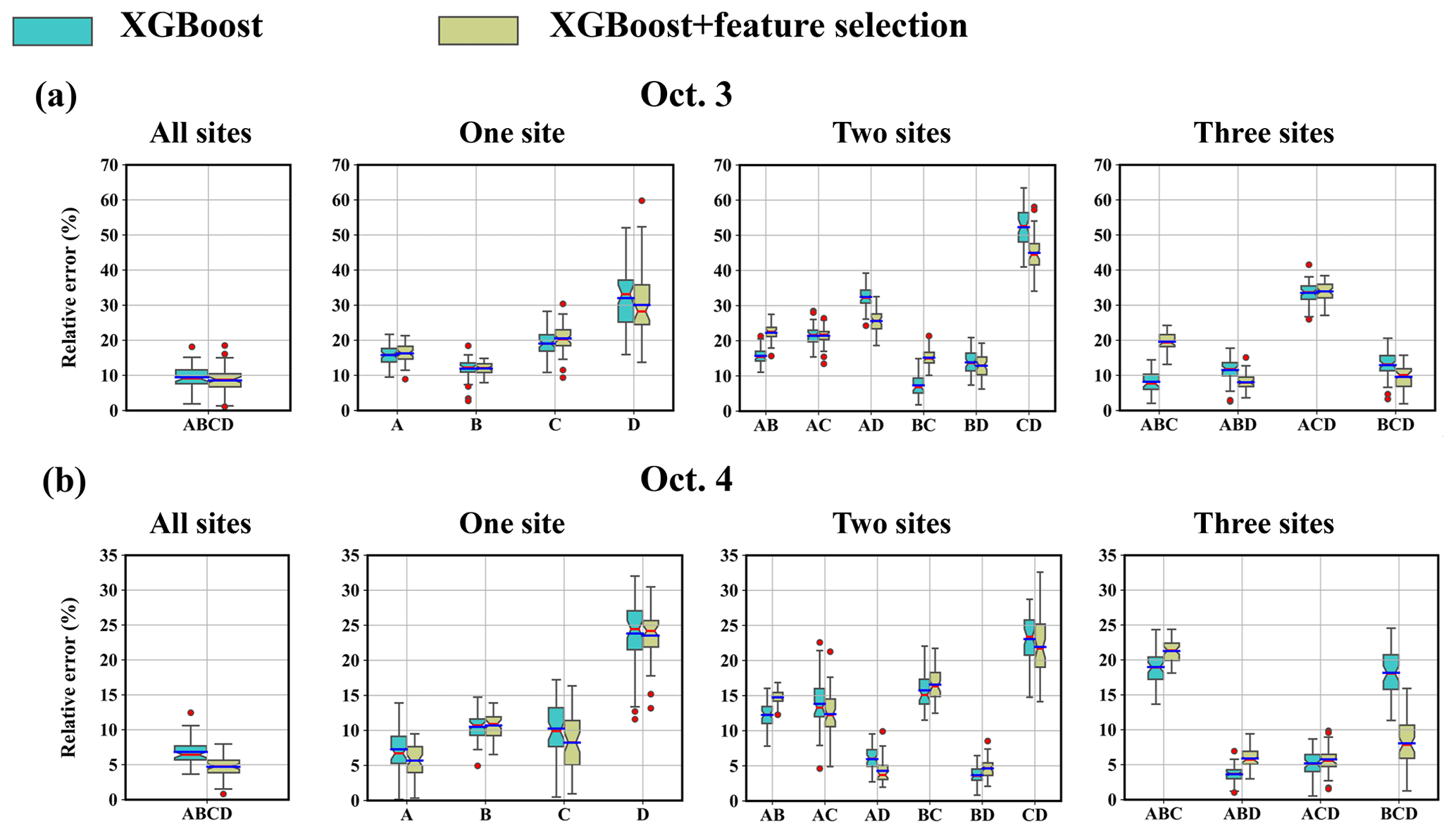
Figure 13 Sensitivity to the number and combination of observation sites. (a) 3 October; (b) 4 October.

3.4.4 Sensitivity to the number and combination of observation sites

Figure 13 compares the results obtained with different numbers and combinations of observation sites. The results indicate that the source-location error may be more sensitive to the position of the observation site than to the number of sites included. The error level of all-site estimations is relatively low for both days, indicating that increasing the number of observation sites better constrains the solution and helps improve the robustness of the model. However, the lowest error levels are achieved by a subset of sites, i.e., Site ABD on 3 October and Site BD on 4 October. This is possibly because including all observation sites may cause overfitting and reduce the prediction accuracy. This overfitting can be alleviated by using only representative sites at appropriate positions which capture the environmental variability and provide clear information for locating the source. For 3 October, multi-site estimations with Site B always produce low error levels, and single-site estimation using Site B also achieves high accuracy. For 4 October, multi-site estimations with Site BD always achieve relatively low error levels. These results demonstrate the importance of using representative sites for source-location estimation. The representative sites (Site B for 3 October and Site BD for 4 October) are consistent with the importance calculated in the feature selection step (Fig. 4), preliminarily indicating the potential of feature selection to identify representative sites. In addition, feature selection reduces the mean error level in most cases.

3.4.5 Sensitivity to the meteorological errors

Figure 14 illustrates the distribution of mean relative source-location errors (averaged across 50 groups of hyperparameters) retrieved with 50 perturbed meteorological inputs. For 3 October, the estimates generally present a low error level (generally below 10 %), and the 50th-percentile error level is lower than the error in the unperturbed results (4.68 %). In comparison, for 4 October, most perturbed results exhibit larger errors (primarily 10 %–20 %) than the unperturbed results (4.71 %), indicating that models for 4 October are more sensitive to the meteorological errors. This sensitivity difference results from the layout of the observation sites (Fig. 2a). On 3 October, the sites were almost perpendicular to the prevailing wind direction, so they captured the plume for a large range of wind directions. In contrast, on 4 October, the sites were basically parallel to the wind direction, so they captured the plume for only a very limited range of wind directions. This result indicates the importance of site layout for robust reconstruction in the presence of meteorological errors. Feature selection slightly changes the mean relative error distribution and its percentiles for both days, indicating that meteorological errors may alter the importance of each feature and reduce the effectiveness of feature selection. In addition to meteorological errors, dispersion errors such as wet-deposition parameterization (Zhuang et al., 2023) may influence the result, but these errors are not dominant in the two field experiments. The handling of such dispersion errors will be investigated in future work.

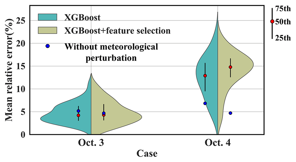
Figure 14 Sensitivity to the meteorological errors. The violin plots illustrate the kernel density estimation of errors obtained with different meteorological groups for XGBoost models before and after feature selection. The vertical black lines inside the violins depict the interquartile range, capturing the 25th, 50th (red dots), and 75th percentiles of mean relative error. The blue dots denote the mean relative source-location errors for models without meteorological perturbation, as listed in Table 4.

4 Conclusions

In this study, we relaxed the unrealistic constant-release assumption of source reconstruction. Instead, we took advantage of the fact that most atmospheric radionuclide releases have a spatially fixed source, and thus the release rate mainly influences the peak values in the temporal observations. Based on this, a more general spatiotemporally separated source reconstruction method was developed to estimate non-constant releases. The separation process was achieved by applying a temporal sliding-window average filter to the observations. This filter reduces the influence of temporal variations in the release rates on the observations so that the relative spatiotemporal distribution of the filtered observations is dominated by the source location and known meteorology. A response feature vector was extracted to quantify the long-term temporal response trends at each observation site, utilizing tailored indicators of both the time and the frequency domains. The XGBoost algorithm was used to train a machine-learning model that links the source location to the feature vector, enabling independent source-location estimation without knowing the release rate. With the retrieved source location, the detailed temporal variations in the release rate were determined using the PAMILT algorithm. Validation was performed against the 2 d SCK CEN ⁴¹Ar field experimental data and two groups of ETEX-1 data. The results demonstrate that the proposed method successfully removes the influence of temporal variations in release rates across observations and accurately reconstructs both the spatial location and the temporal variations in the source.

For the local-scale SCK CEN ⁴¹Ar experiment, the source location was reconstructed with errors as low as 0.60 % (3 October) and 0.80 % (4 October), significantly lower than for the correlation-based method and Bayesian method. In terms of the release rate, the PAMILT method reconstructed the temporal variations, peak, and total release with high accuracy, thus avoiding the unrealistic oscillations given by the Bayesian estimate. The proposed method produced smaller uncertainty ranges than the Bayesian method and avoided the multimodal distribution of the Bayesian method. The feature selection process removed the redundant features and reduced the reconstruction errors. For the continental-scale ETEX-1 experiment, the lowest relative source-location errors were 0.20 % and 0.70 % for Group 1 and Group 2, respectively, which were again lower than those for the correlation-based and Bayesian methods. The proposed method provides highly accurate mean estimates of the release rate for both groups, although with a large uncertainty range.

Sensitivity analyses of the SCK CEN ⁴¹Ar experiment revealed that the proposed method exhibits stable source-location estimation performance with different parameters and remains effective with only a single observation site, as long as the selected site is appropriately located. Moreover, the proposed method shows robust source-location estimation in the presence of meteorological errors, with mean source-location error levels below 10 %, on the condition that the site layout is appropriate.

These results demonstrate that spatiotemporally separated source reconstruction is feasible and achieves satisfactory accuracy in multi-scale release scenarios, thereby providing a promising framework for reconstructing atmospheric radionuclide releases. However, the proposed method does not consider the influence of temporal variations in the release rate on the plume shape. Our future efforts will be directed towards integrating spatial features to further enhance the method.