An open-source refactoring of the Canadian Small Lakes Model for estimates of evaporation from medium-sized reservoirs

Eddy covariance (EC) is one of the most effective ways to directly observe evaporation from a lake surface. However, the deployment of EC systems on lakes is costly and technically challenging, which engenders a need for accurate modelling of evaporation from reservoirs for effective management. This study aims to (1) refactor the Canadian Small Lakes Model (CSLM) into modern high-level programming languages in open-source repositories and (2) evaluate evaporation estimates from the CSLM using 9 years of EC observations of a pit lake in Northern Alberta. The CSLM is a 1-D physical lake model simulating a mixing layer and an arbitrary thick skin layer which interfaces with the atmosphere and includes a module for ice dynamics. It was developed to interface with the Canadian global coupled models as part of the surface classification scheme and thus utilizes widely accessible forcing data. In this study the CSLM evaporation estimates are also compared to a commonly used bulk transfer method of estimating evaporation. In general, the CSLM had smaller open-water season error (RMSE of 0.70 mm d⁻¹) than the bulk transfer method (RMSE of 0.83 mm d⁻¹). However, if EC data are available, further improvement can be gained by using an artificial neural network to adjust the modelled fluxes (RMSE of 0.51 mm d⁻¹). This final step can be very useful for gap-filling missing data from lake observation networks as there has been recent attention on the limited coverage of direct open-water evaporation observations in the literature.

1 Introduction

Globally, the volume of water stored in reservoirs used for hydroelectricity production as well as water and waste management has been increasing. Managing these reservoirs is complex, and one of the largest uncertainties is the quantification of evaporation (Long et al., 2007), which is rarely measured. Direct observation of the evaporative fluxes over small and large bodies of water is uncommon due to logistical difficulty, safety, cost, and power availability. When observations are made, it is typically during the warm open-water season with less of an emphasis on the cooling phase of the year when evaporation is greatest (Rouse et al., 2005; Blanken et al., 2011). The bias in observations of northern lakes towards warm stratified periods results in a limited understanding of the drivers of evaporation variability for reservoir managers. Complete observation records of the ice-free season are important since prior work (e.g. Spence et al., 2003; Lenters et al., 2005; Granger and Hedstrom, 2011; Spence et al., 2011; Liu et al., 2012; Shao et al., 2020; Fournier et al., 2021) has shown significant differences in atmospheric forcing that drive evaporation processes between the warming, cooling, and frozen phases of lakes. Here warming is broadly defined as the spring mixing and stratification period when the atmosphere is generally warmer than the lake, cooling is turnover when the lake is warmer than the air, and frozen is the ice-covered period.

In addition to the management implications, variability in the rate of evaporation has regional impacts on the atmospheric conditions since bodies of water alter the climatology of landscape (Rouse et al., 2005; Long et al., 2007; Blanken et al., 2011). In landscape-scale reclamation projects, such as those in the Athabasca oil sands region, variation in surrounding atmospheric conditions directly impacts the landscapes surrounding water bodies and should be considered in the reclamation plan. Lakes contribute to increased humidity and alter the seasonality of surface energy storage and exchange. In general, the mixing dynamics and large heat capacity of water bodies result in a surface that is slower to heat and slower to cool than surrounding terrain. This differential in the thermal momentum of lakes produces large sensible and latent heat fluxes to the atmosphere during the cooling season. In large northern lakes, which remain mostly ice-free, up to 88 % of the annual evaporative flux occurs over the cold months (Blanken et al., 2011). Even in smaller lakes, or large lakes that completely freeze, the cooling period prior to ice formation represents the most significant period for water loss to the atmosphere (Clark et al., 2021). Although studies of direct lake evaporation have been increasing in recent years, the period prior to ice formation remains difficult to measure due to the complications in both personnel safety and mechanical damage to instruments that lake ice causes in field-based research programmes.

Broadly there are three typical approaches to estimating evaporation from widely available, or easily measured, meteorological data: aerodynamic/bulk transfer methods, radiation-based estimates, and empirical equations (Fournier et al., 2021). The bulk transfer method is derived from Dalton's law and Monin–Obukhov similarity theory and is based on the drying power of air as a function of turbulence and humidity (e.g. Heikinheimo et al., 1999). Due to the need to estimate turbulent conditions, this method requires the most localized meteorological observations. Radiation-based methods primarily include available energy, which is more consistent over large areas, especially when surface radiative properties are consistent (e.g. Shuttleworth, 2012) and are accurate at daily flux timescales or longer (Granger and Hedstrom, 2011). Empirical equations are typically derived from regressions to available data (e.g. Granger and Hedstrom, 2011). Both of these later methods have more flexible data requirements than the bulk flux transfer method, but the trade-off is a greater uncertainty in extrapolating beyond the conditions for which they were developed. There are several hybrid approaches or “combination equations”, but they are variations on the above approaches. In general, due to the distinct differences in drivers of evaporation between the warming and cooling phases, the most accurate estimates of evaporation come from approaches utilizing localized wind speed and surface temperature estimates (Fournier et al., 2021). In addition to localized data, this paper aims to also highlight the advantage of using a process-based model for estimating evaporation rates from managed northern reservoirs. A mechanistic model can provide not only evaporation estimates, like the above approaches, but it also provides insight into lake processes that could be valuable to managers and researchers, such as turnover timing(s), ice formation and season length, total energy storage, shear and buoyant forces, thermal profile, and depth to thermocline.

For both water resource management and for evaluating the impact of climate change there is an emergent need to be able to accurately quantify the lake–atmosphere flux of water and energy. Here we compare two methods, the air–sea toolbox developed by Fairall et al. (1996) and the Canadian Small Lakes Model (CSLM) developed by MacKay (2012). The first, the air–sea toolbox, is a bulk flux algorithm developed for Tropical Ocean-Global Atmosphere (TOGA) Coupled Ocean Atmosphere Response Experiment (COARE). The second, the CSLM, is a one-dimensional dynamic model developed for inclusion with the Canadian Land Surface Scheme (CLASS) to be used in the Canadian Global Coupled Model (CanGCM) and Environment and Climate Change Canada's numerical prediction systems. Here we present (1) the refactoring of the CSLM to high-level languages and open-source distribution for use by scientists and land managers who may have limited modelling expertise and (2) an assessment of these two modelling approaches for estimating northern lake–atmosphere exchange with almost a decade of direct eddy-covariance-based lake–surface flux observations.

2 Methods

2.1 Study site

Base Mine Lake (BML) is located on the Syncrude Canada Ltd Mildred Lake mine lease in Northern Alberta, Canada (Köppen climate Dfb, boreal plains ecozone). Over the study period, BML typically had a total ice cover by early-to-mid November, and it melted by late April/early May. BML is a reclaimed pit lake, built on an active oil sands pit mine. The lake and surrounding topography were constructed from pit infill and overburden to be the terminus of a constructed 660 ha watershed of upland forests and peat-filled lowlands. From 1994 to 2012, fluid fine tailings (FFTs; by-products of the oil sands mining process) were stored at the site to a depth of 45 m with an additional 3–5 m freshwater capping. In 2012, the water capping was increased 8–11 m to initiate the reclamation of the lake in the freshwater cap. The exact quantity of freshwater varies as the lake is highly managed, with freshwater regularly added and removed during mine operations (Clark et al., 2021, for more details of water management). The volume of water additions (sourced from a nearby lake with a similar surface temperature) are unlikely to significantly impact the overall energy budget due to the relative volume (mean of 3.2 % of the total lake volume and declining over the study period). The FFTs have greatly consolidated and “dewatered” into the lake column, producing a semi-solid bottom layer under the freshwater capping. Alum treatments used to clarify BML in late 2016 led to the formation of a precipitated fine-sediment layer between the freshwater and FFTs, sometimes referred to as the “mud layer”. This layer is regularly re-mixed within the water column, leading to large variability in the turbidity of BML (Tedford et al., 2019). Early in the reclamation, the lake had a noticeable amount of residual hydrocarbons that produced a sheen, which likely impacted latent energy fluxes by buffering kinetic energy transfer and wave formation or by forming a thin barrier between the water and the atmosphere (Clark et al., 2021). More recently, however, lake water quality has improved through management activities such as mechanical skimming of the surface and the above-mentioned alum treatments.

An eddy covariance platform is ∼ 1 km from the nearest shore so is unlikely to suffer edge effects (Kenny et al., 2017). The large moored 6 m by 6 m steel observation platform is stable, except in extreme waves. The EC system was comprised of a infrared gas analyser (LI-7200) and a three-dimensional sonic anemometer (Gill WindMaster Pro). Corrections to compensate for low- and high-frequency losses were performed via the methods in Moncrieff et al. (1997). Observations from the infrared gas analyser also required corrections to compensate for density fluctuations (Webb et al., 1980). Corrections and 30 min bulk-averaged fluxes were computed using the EddyPro software package (version 7.0.8, LI-COR, Inc.). All fluxes of poor quality, according to the methods of Foken et al. (2004), were removed from the analysis. The EC system operated year-round, although solar power became difficult to maintain in the darkest months, resulting in limited observations throughout the December–February period. A full description of the platform and the methods used to derive the eddy covariance observations used to validate the surface models can be found in Clark et al. (2021). To ensure high-quality data, observations within a 140° arc containing the platform are excluded from this analysis. Lake temperatures were directly observed at depths of 0.1, 0.2, 0.5, 1, 3, 4, 5, 6, 7, and 8 m at various intervals throughout the study period. To validate the CSLM simulated temperature profile, the observed temperature profile was linearly interpolated in 0.5 m increments from 0.5 to 8 m to align with the lake layers in the CSLM. The mean temperature difference of simulated layer from this interpolated observation record is reported for each depth and as a total water column mean error.

2.2 Meteorological forcing

Both models require atmospheric forcing data. Direct observations were used when possible, yet there were missing periods when equipment was malfunctioning or access to the lake platform was limited. Gaps in the meteorological datasets are filled by linear relationships to the NCEP reanalysis 2 product produced by NOAA (Kanamitsu et al., 2002) after first downscaling the reanalysis data to a 30 min time step. These datasets are available here: https://psl.noaa.gov/data/gridded/index.html (last access: 13 June 2024).

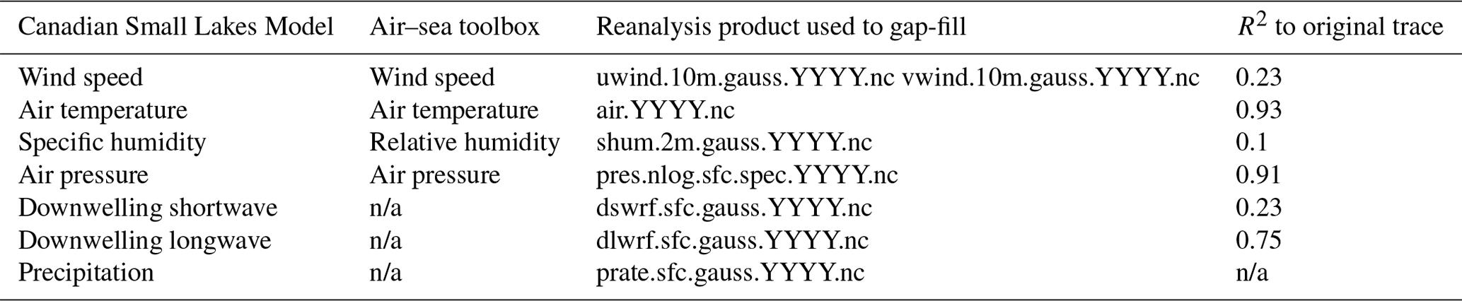
By default, the CSLM integrates over a 600 s time step. Therefore, gap-filled observations were linearly interpolated from 30 to 10 min records for the CSLM simulations. The specific observations used to force the model and the data source are listed in Table 1.

Table 1 Meteorological variables used in forcing the two models. Precipitation has no R² as the reanalysis value was used directly when there were gaps in the local data. n/a – not applicable

2.3 Model descriptions and run settings

The CSLM (MacKay, 2012; MacKay et al., 2017) was refactored to provide fluxes to interpolate missing data from surface–atmosphere eddy-covariance-based reservoir observations. The CSLM was initially developed to fit into the Canadian Land Surface Scheme (CLASS; MacKay, 2012) to enable the inclusion of lake surfaces in the Canadian global coupled models for climate simulation. Lakes have historically been absent from global coupled models' (GCM) simulations, and only recently has their inclusion in land surface models been considered (Fisher and Koven, 2020). Briefly CLASS divides each grid cell in the GCM into fractions of surface types and structures to feed back mechanistic behaviours of the earth surface into the atmospheric models. Since CLASS functions on fractional surface area of each grid cell, it is not constrained by the model's resolution. The CSLM is a 1-D simulation of the lake surface–atmosphere interaction of any depth divided into user-defined layers. By collapsing the simulation to the vertical dimension, the physics that govern surface temperature through wind-shear-induced mixing, variable light attenuation, buoyancy, and ice development are simplified. When included in larger simulations the modelled lake surface energy exchange is scaled to the fraction of the open-water area in the grid cell like in CLASS. This allows the CSLM to work independently or within any simulation that works with CLASS and produces a more accurate estimate of ice extent, total cover, and surface temperature of small and mid-sized lakes when compared to the simple water scheme used in Canadian climate models or numerical prediction systems (Garnaud et al., et al., 2022).

The FORTRAN 77 codebase for the CSLM has been provided by a developer (Murray MacKay, Environment and Climate Change Canada) and contains all the machinery to embed CSLM within CLASS. FORTRAN has limited use outside the earth system model community, and older iterations are increasingly difficult to access and compile. Conversely, high-level languages such as MATLAB and Python are widely taught and applied in earth system sciences, and translating the CSLM codebase will allow its application outside climate modelling and numerical prediction systems. Furthermore, in refactoring CSLM, modern programming practices can be implemented, and GOTO and historical design patterns can be replaced with modern structured practices. Although high-level languages often compromise on efficiency with greater overhead in data management, the computational requirements to run CSLM on one lake is low on modern processes (< 1 min per simulated year on a desktop PC). In addition, refactoring allows unlimited variable length names and white spaces that make the codebase more intuitive for those who wish to modify or add features (i.e. the name for the latent heat flux from the lake surface is now LatentHeatFlux in both MATLAB and Python compared with HEVLGAT in FORTRAN). A complete list of translated variable names from FORTRAN is listed in Table S1 in the Supplement.

The CSLM requires the lake latitude, longitude, depth, length, initial temperature profile, instrument observation height, and extinction coefficient (how rapidly light is absorbed in the water column). These parameters can be set via the MakeLakeINI() function in the provided code. For this project, the light extinction varied seasonally and was set to 0.2, 0.3, 0.25, 0.2, 0.15, 0.05, and 0.05 for May through November, respectively, and 0.1 for all other months. These values were determined by running the CSLM with a fixed extinction coefficient at 0.05 intervals from 0.05 through 0.4 and determining the minimum mean squared error of the top 1.5 m of the lake profile from the observed for all years. The code is also set up such that if no variable extinction coefficients are given, the user may specify a fixed value in the MakeLakeINI() function. At each time step the option to override the simulated lake temperature profile with direct observations was also added to the CSLM model. If the input observations are missing, not sampled at high enough frequency, or if none are provided, the model will use the simulated profile instead.

The air–sea toolbox (Fairall et al., 1996) MATLAB implementation was obtained from the GitHub repository (https://github.com/sea-mat/air-sea, last access” 13 June 2024). It was run without the cool-skin module and with four of the same atmospheric forcing variables as the CSLM (see Table 1). Surface temperature used in the forcing of the air–sea toolbox was derived from the upwelling longwave radiation and Stefan–Boltzmann law.

Finally, a five-node artificial neural network (ANN) to estimate evaporation from BML was trained using both models, the same atmospheric variables as required to run the CSLM, the year of observation, and two seasonal vectors. The seasonal vectors are simply cos(X) and sin(X), where X is day of year divided by 365 multiplied by π. The ANN scales the training data from min/max to $-\mathrm{1}/\mathrm{1}$ and a hyperbolic tangent sigmoid is used for the transfer function between the nodes. Training is done through the Levenberg–Marquardt error back propagation. The ANN is trained on 50 % of the data, with 25 % set aside for validation and 25 % set aside for testing. The adjusted R² of the ANN output to the testing data was 0.67 for latent heat and 0.72 for sensible heat. A permutation importance analysis is included as Fig. S1 in the Supplement.

2.4 Analysis

To test the performance of the model in simulating lake dynamics, the model was run continuously from 1 January 2013 to 31 December 2021 without overriding the lake temperature profile. The resulting profile was compared to observations to assess the accuracy of the simulated lake temperature profile.

2.4.1 Computation of daily-scale fluxes from half-hour observations and simulations

In the analysis of daily-scale observations, days are the sum of the half-hour observations and simulations. Sensible heat flux is in J, and the latent heat flux has been converted into millimetres of water using the average air pressure and temperature of the half-hour flux. Days with less than 36 half-hour observations were not included in the analysis. Days with less than 48 half-hour observations, but more than 36, had the missing data filled with linear interpolation before calculating the daily flux. Seasonal total evaporation was calculated for the CSLM, air–sea toolbox, and the ANN gap-filled observed latent heat flux.

2.4.2 Comparisons of simulated and observed fluxes

Comparisons of half-hourly and daily modelled sensible and latent heat fluxes are done with ordinary least squares regression (OLS). Seasonal bias was evaluated by plotting the coefficient of determination (R²) from OLS performed on data grouped by each month of the year. In addition to the R², for more direct visual inspection, the mean daily evaporation rate for all years was plotted by DOY for all simulated and observed fluxes. So as not to change the sample depth for the mean calculation between modelled and observed fluxes, only days when an observed flux was available were used for all three plots.

2.4.3 Error analysis

Throughout this analysis the term “error” was used explicitly as the observed value minus the modelled value divided by the observed value. This prevented the error analysis from being skewed towards the largest fluxes. A boxplot was generated for the error from each model in each month of the year. Errors are then evaluated with respect to the state of the atmosphere (turbulent kinetic energy, TKE; friction velocity, u_∗; Obukhov length, OL; and vapour pressure deficit, VPD). For visual clarity, error terms are binned to the corresponding atmospheric state variable and plotted as boxplots. The bins are determined by 5 percentile ranges, such that the first bin is all the fluxes that correspond to < 5th percentile, the second bin is ≥5th through < 10th, and so on. Analysis of the error was also conducted using wind speed, as wind speed is a widely measured variable unlike the more micro-meteorological specific variables described above. For simplicity in the wind speed error analysis the error was grouped in 1 m s⁻¹ bins instead of percentiles.

2.4.4 Analysis of the simulated seasonal ice coverage

Finally, to evaluate the ice module of the CSLM, ice-free days were compared to the observed days of ice-on and ice-off when it was available. Then the total evaporation was compared to the number of predicted ice-free days along with average daily temperature, average relative humidity, and average wind speed for the same period. OLS was used to assess any relationship between evaporation rates and ice-free periods, as well as average temperature.

3 Results

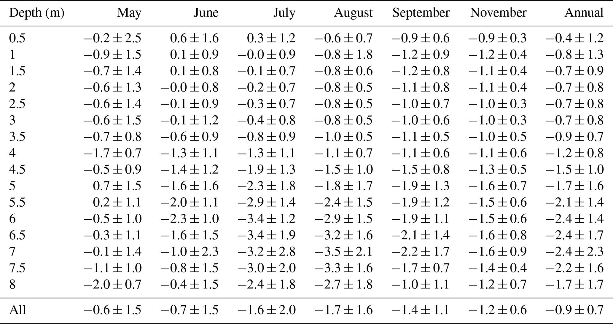
When run without the lake temperature observations overriding the simulation, the CSLM modelled temperature of the water column overestimates the observed water column by 1.3 ± 1.3 °C for all the periods and depths for which water column temperatures are available (Fig. 1; Table 2). However, the observations are not evenly spread across the season, and August and September are more represented than May, June, and July periods. The upper 3 m of the simulated profile is much closer to the observations (mean temperature difference of 0.6 ± 1.0 °C) than the deeper layers (mean temperature difference of 1.6 ± 1.3 °C for 3.5 to 8 m) (Fig. 1; Table 2). It should be noted that the extinction coefficient was calibrated on the 1.5 m depth, so it likely has to do with the accuracy over this region. Fall turnover is well captured by CSLM with respect to the lake temperature profile, but the simulation is still warmer (mean difference of 1.2 ± 0.6 °C for 1 September to 31 October).

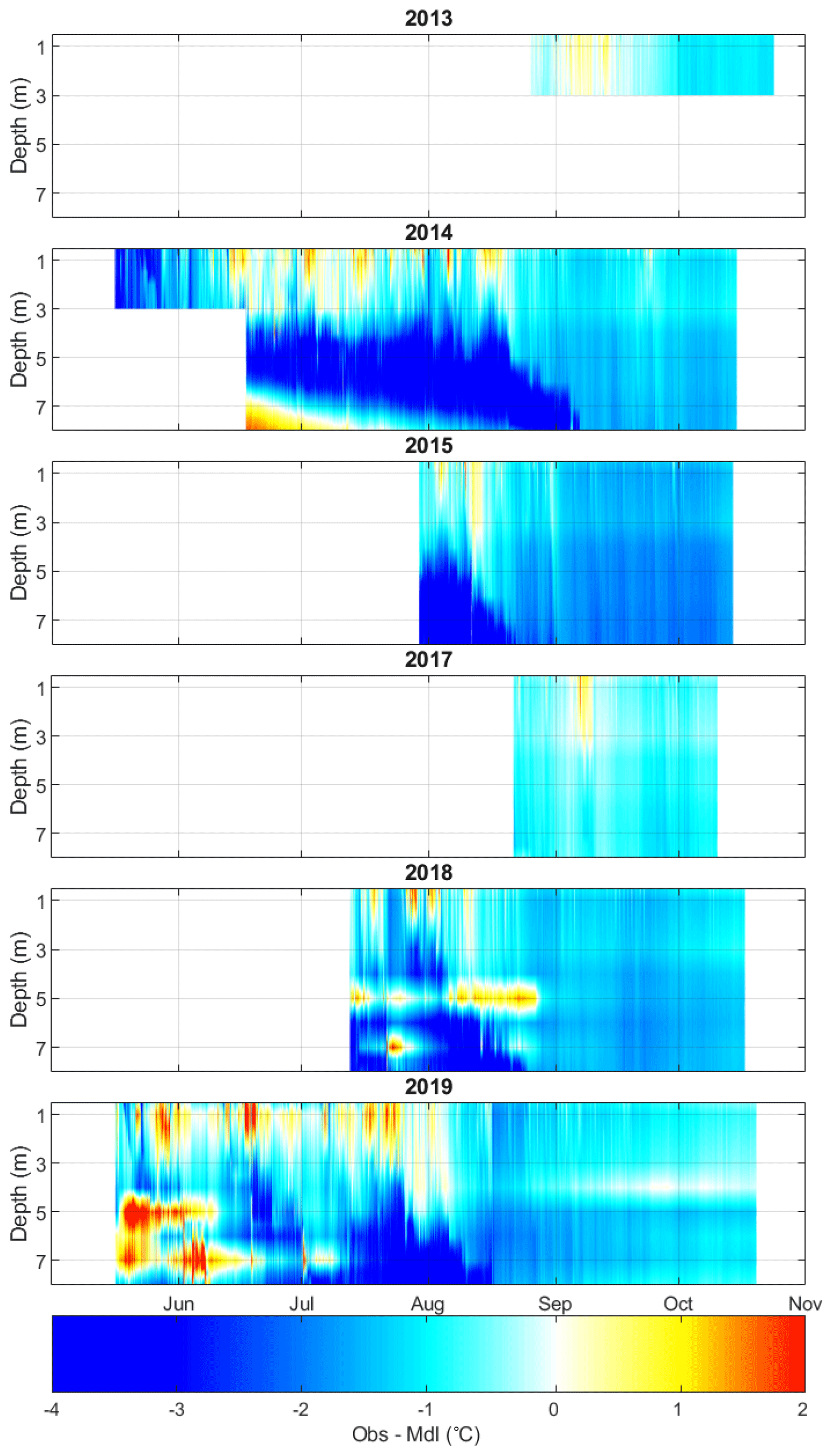
Figure 1 Difference between the observed and Canadian Small Lakes Model (CSLM) estimated BML lake temperature profile for when the CSLM was run without overriding the lake temperatures with the observed temperatures.

Table 2 Mean temperature difference between observations and each lake layer of the Canadian Small Lakes Model (CSLM) run without overriding lake temperatures. Negative values indicate that the CSLM overestimated temperatures, while positive values indicate an underestimate.

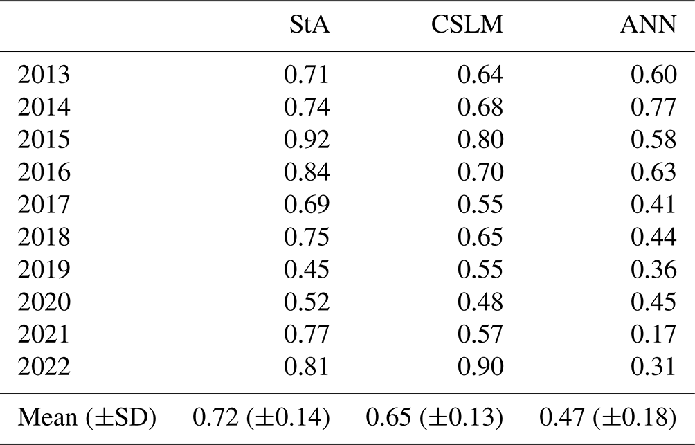
The half-hour latent heat fluxes from the CSLM and the air–sea toolbox approximated the observed fluxes (R² of 0.60 and 0.56, respectively, p value < 0.001; Fig. 2). However, the ANN increased the accuracy substantially (R² 0.69, p value < 0.001). The modelled daily total evaporative flux was closer to the total observed daily flux for all the models (R² of 0.76, 0.83, and 0.91 for the air–sea toolbox, CSLM, and ANN, respectively; Fig. 2). The models are better at approximating the larger-scale trends and have better accuracy at the daily scale (as measured by R²) and slopes closer to 1 (Fig. 2). Like the lake temperature profiles, the half-hour (and daily) estimates generally improved in recent years compared to the early years (Table 3). In relative units, the root mean squared error for the daily estimated evaporation rate for the whole study period was 0.83, 0.71, and 0.52 mm d⁻¹ for the air–sea toolbox, CSLM, and ANN, respectively (see Table 3 for interannual breakdown).

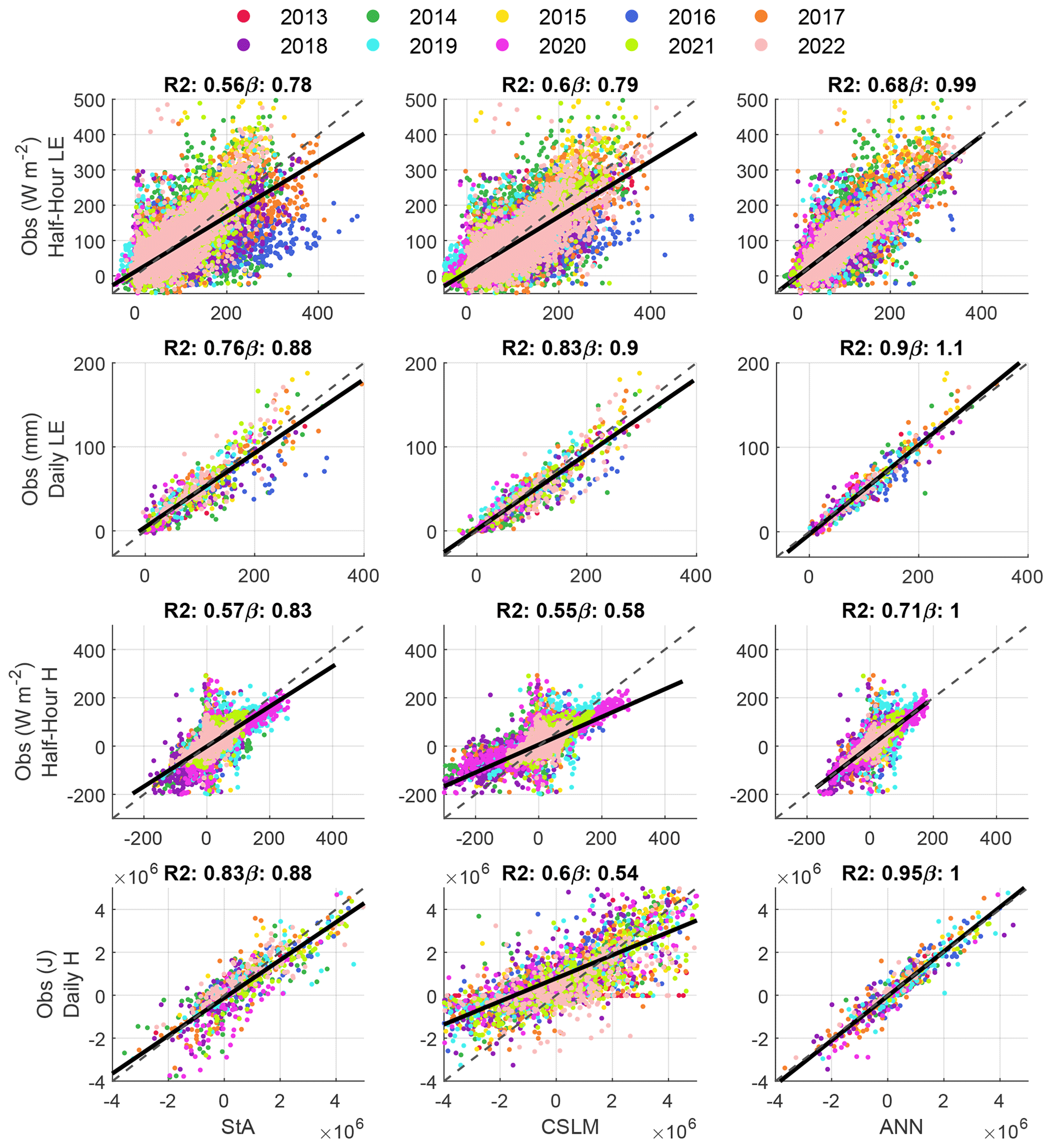
Figure 2 Scatter plots of the modelled and observed heat fluxes at both the half-hour and daily scales for the air–sea toolbox (StA), Canadian Small Lakes Model (CSLM), and artificial neural network (ANN), respectively. Dashed lines are 1:1 lines, and solid lines are regression lines. The top row shows half-hour latent energy fluxes (LE), the second row shows daily latent energy fluxes, the third row shows half-hour sensible heat fluxes (H), and the bottom row shows daily sensible heat flux. R² and the slope of the regression line (β) are given above each plot. All regressions are significant with p values < 0.001.

Table 3 Root mean squared error (mm d⁻¹) between observations and the air–sea toolbox (StA), Canadian Small Lakes Model (CSLM), and artificial neural network (ANN), respectively. The number of observations varied each year.

Estimated sensible heat flux followed a similar trend to the latent heat flux at the half-hour scale (R² of 0.57, 0.55, and 0.71, p value < 0.001, for air–sea toolbox, CSLM, and ANN estimates, respectively). At the daily scale, the modelled fluxes more accurately estimated the observed flux variability (R² of 0.83, 0.6, and 0.94, p value < 0.001, for air–sea toolbox, CSLM, and ANN estimates, respectively), but only the ANN estimated sensible heat fluxes were close to 1:1 (Fig. 2). Notably, in 2019 and 2020 there were several near-zero estimated sensible heat fluxes when the eddy covariance observations spanned the whole range of reasonable values (Fig. 2). The comparison of the accuracy between modelled and eddy covariance observed data can become problematic in certain atmospheric conditions and is discussed more below.

Each model's performance also has a seasonal bias. Frozen season fluxes are poorly estimated, but that may be a consequence of limited observations to compare to (Figs. 3 and 4). Estimated latent heat fluxes in the spring (March, April, and May) have the lowest relative accuracy of the year for all models (Fig. 4). The early warming period (May for BML) also has the lowest R² values, which increase throughout the ice-free season (Fig. 3). The relative error in the spring is somewhat reduced, and the median is closer to zero for the ANN estimated fluxes, but the error is still much higher in the spring than the rest of the year. These low relative errors do not accumulate substantially in the total seasonal evaporation rates as spring fluxes are quite low compared to those in the fall (Fig. 4). The coefficient of determination between estimated and observed fluxes improves throughout the year until ice onset sometime in November (Fig. 3). The CSLM tends to predict higher surface-to-atmosphere latent heat transfer during the warming phase and lower during late fall before ice onset (Fig. 4).

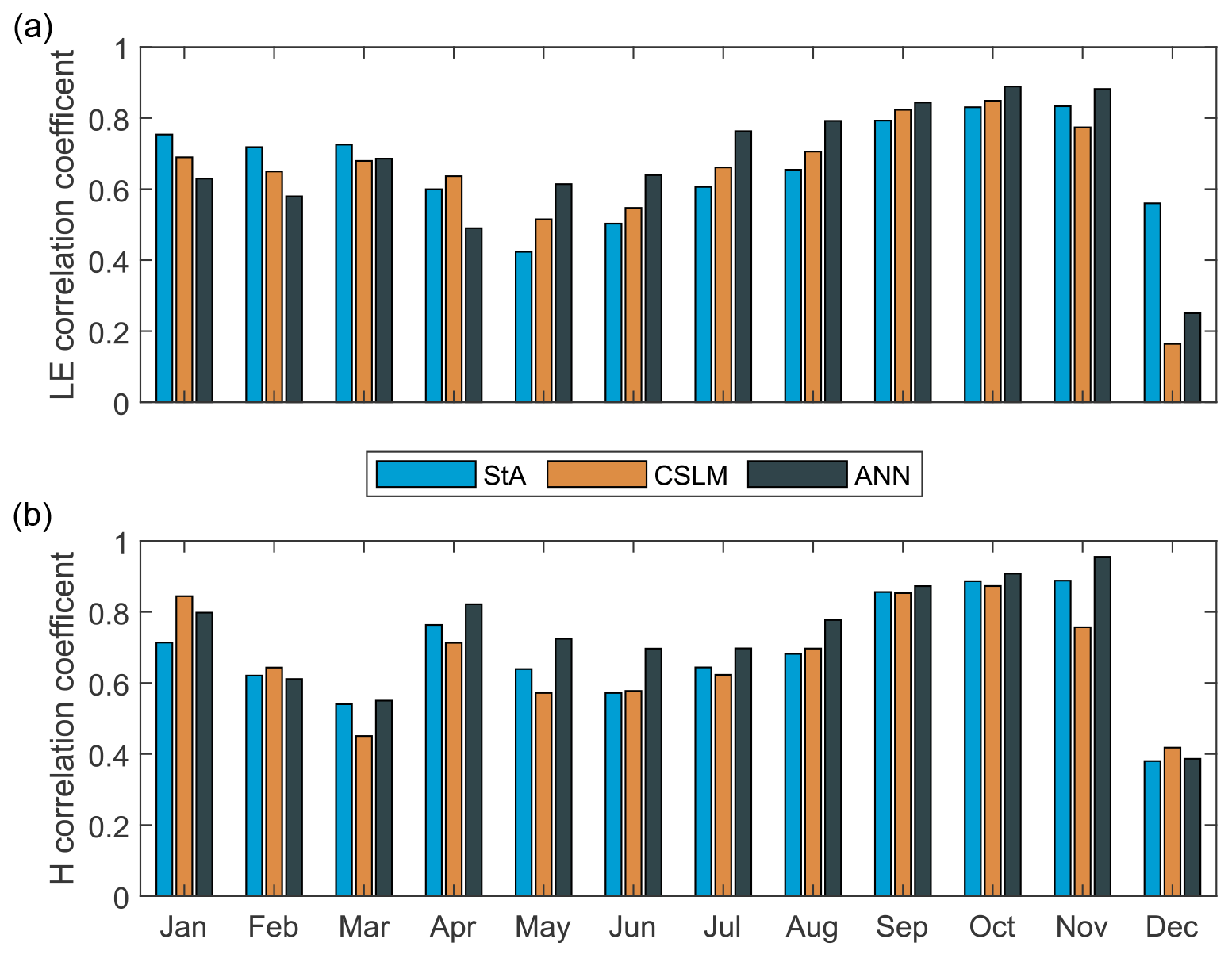
Figure 3 Coefficient of determination between model-predicted latent heat flux (a) and sensible heat flux (b) for each month pooled across all years (left) for the air–sea toolbox (StA), Canadian Small Lakes Model (CSLM), and artificial neural network (ANN), respectively. All values are significant (p values < 0.0001) except the latent heat fluxes from CSLM in December (p value = 0.52) and ANN in January (p value = 0.01).

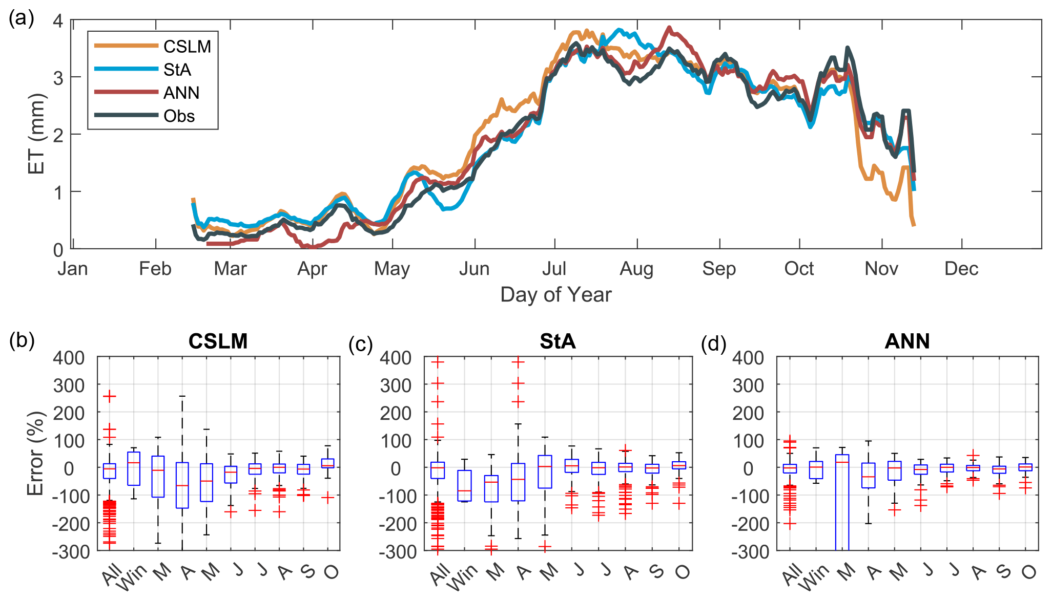
Figure 4 (a) The average daily flux over the 9 years of observations. Bottom monthly error rates of the models (observation − estimation). In panel (a), for comparability the air–sea toolbox (StA), Canadian Small Lakes Model (CSLM), and artificial neural network (ANN) estimated evaporation rates were only included if there was a corresponding daily observed value. Boxplots show the median (red line), interquartile range (blue box), 5th to 95th percentile range (whiskers), and outliers (red +).

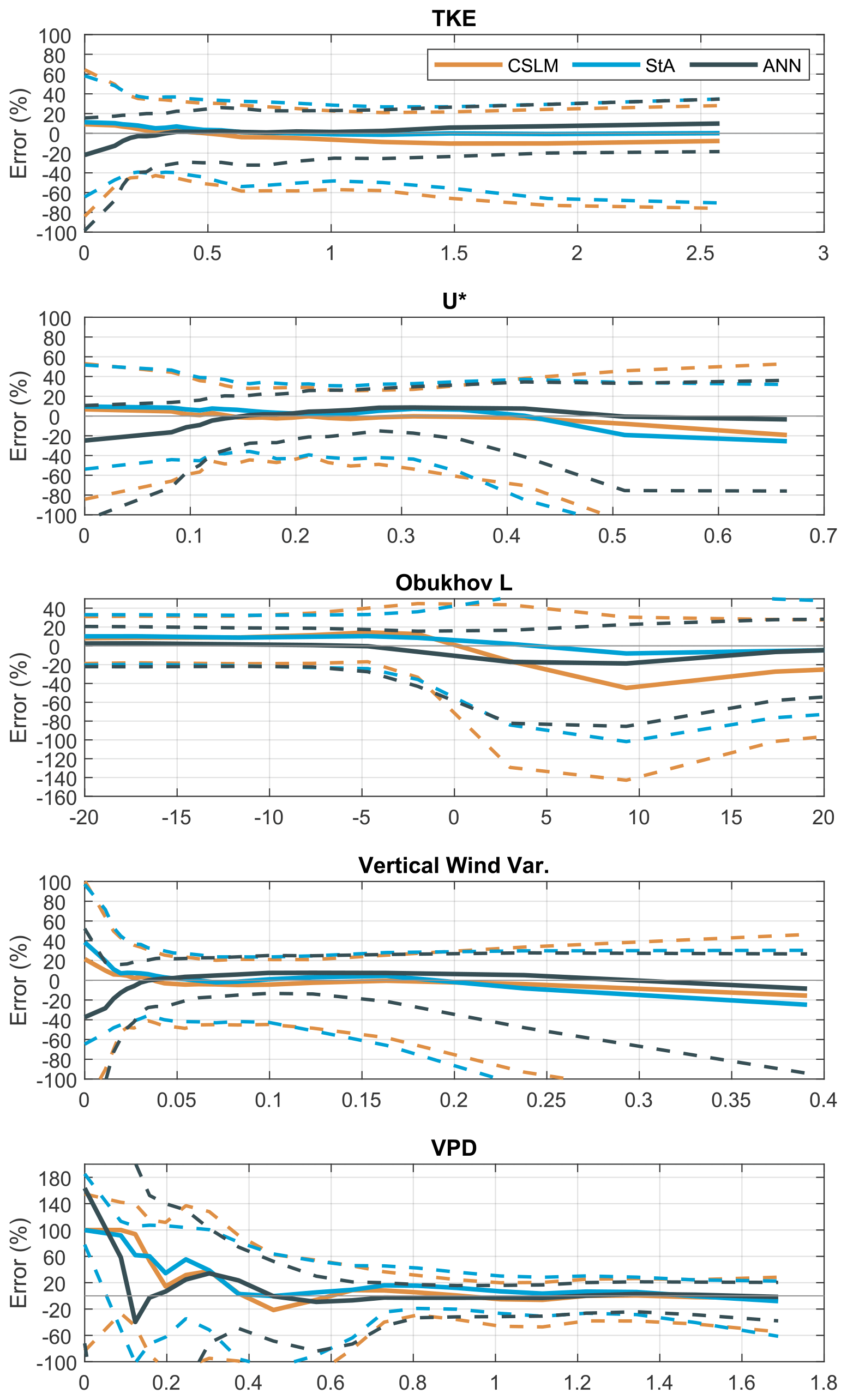
Figure 5 Error [(observed − modelled)$/$observed × 100 %] as a function of atmospheric turbulence, stability, and vapour pressure deficit. Solid lines are the median value, and dashed lines cover the interquartile range.

The typical accuracy in response to the state of the atmosphere was consistent. Both the CSLM and the air–sea toolbox estimated fluxes had much lower accuracy when there was limited kinetic energy in the atmosphere (i.e. when the atmosphere was stable). Low total kinetic energy, friction velocity, vertical and cross wind variance (not shown), and positive near-zero Obukhov length increased the error of the model output compared to the observed fluxes (Fig. 5). The ANN did not provide much improvement during these conditions and showed median errors in excess of the other models when there was limited mixing (low TKE, u_∗). There was a slight increase in the median error as a function of u_∗ (Fig. 5), suggesting that at high friction velocities the models underestimated the latent heat flux. All three models were relatively accurate at high VPD when evaporation is highest but had greater error in humid conditions (Fig. 5). For more general interpretability outside of a micrometeorological analysis, the error associated with atmospheric turbulence and stability can be approximated by low wind speeds (Fig. 6). At high wind speeds the models tend to overestimate the rate of evaporation, and at low wind speeds they underestimate it (Fig. 6). It should be highlighted that the median ANN latent heat flux compensates for this error because wind speed is part of the training data for the ANN and therefore has already adjusted the latent heat flux based on the typical offset unlike the above micrometeorological variables. However, the variance in the error from the ANN simulated heat flux is still high at low wind speeds (Fig. 6).

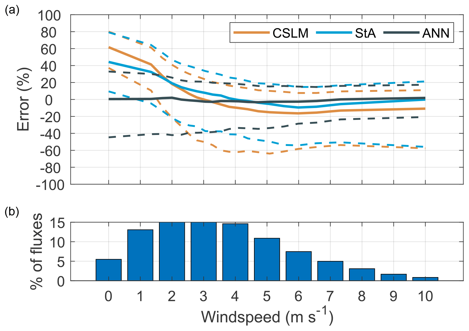
Figure 6 Panel (a) is the model error and panel (b) is a histogram of the fluxes as grouped by wind speed (m s⁻¹). Dashed lines represent the interquartile range, and solid lines are the median error.

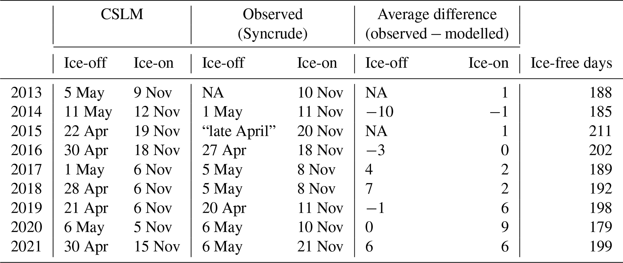
Annually the CSLM and air–sea toolbox was within 11 ± 85 mm and 27 ± 54 mm of the seasonal evaporative flux of 452 ± 58 mm (Fig. 7). In addition to the high seasonal accuracy, when run continuously for the whole 2013–2021 periods, using the lake profile data when available, the CSLM simulates the length of the ice-off season within a few days. Specifically, the CSLM predicted 0.4 ± 5.9 d early for ice-off and 2.9 ± 2.2 d early for ice-on, resulting in an average open-water season 3.0 ± 5.9 d shorter than what was observed (Table 4).

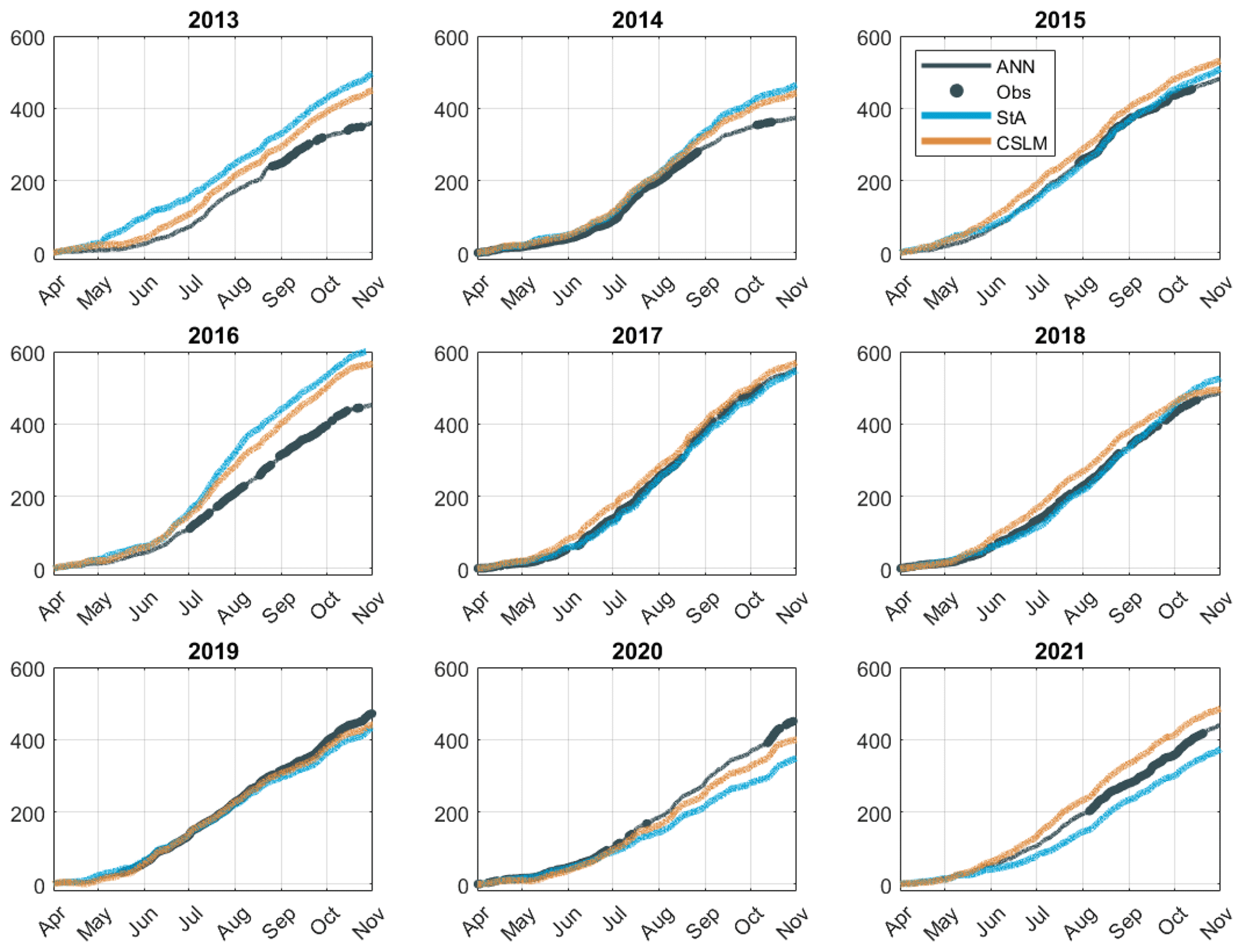
Figure 7 Cumulative sum (mm) of evaporation from BML. For the cumulative sum of the observed fluxes, the gaps were filled with the ANN model.

Table 4 The Canadian Small Lakes Model (CSLM) simulated vs. observed day of ice breakup and ice onset. Average accuracy of the CSLM is 0.1 ± 6.1 d early for ice-off and 2.4 ± 2.1 d early for ice-on. Ice-free days are calculated from the CSLM data. NA – not available

4 Discussion

The first objective of refactoring CSLM now has code available on GitHub as open-source codebases in both Python (https://github.com/mclark04/CSML_Python, last access: 19 December 2023) and MATLAB (https://github.com/mclark04/CSLM_MATLAB, last access: 19 December 2023). They have been written such that the logic is more consistent with modern high-level coding patterns and the variable names are all in camel case to make it more intuitive. The second objective of assessing the modelling approaches is more complex, and below we discuss the advantages and disadvantages of the three modelling approaches.

BML is an oil sands pit lake that is highly managed, has had variability in turbidity that spans orders of magnitude, has been impacted by hydrocarbons, and has tailings, not mud or bedrock, as its bottom. Although the turbidity has become lower and less variable since the alum treatment in 2016, the large variability in turbidity during the early years likely caused the larger errors in the top 3 m of the temperature profile and the resulting latent energy fluxes simulated by the CSLM. The refactored code can accommodate a continuous extinction coefficient, but the turbidity data for BML were not continuously available. In the early years, BML had a notable hydrocarbon sheen (Clark et al., 2021). Hydrocarbons on water can create a barrier between the atmosphere and the water surface and momentum (sheer) transfer into the water (i.e. waves). Exactly how this impacts the latent energy flux for a mid-sized lake is an area of ongoing research, but it likely contributed to the early years' error in the surface atmosphere exchange. Finally, there are two irregular conditions in BML that may cause bias that other lakes do not have. First, below the mud layer in BML there are fluid fine tailings, not sediment/bedrock as assumed in the CSLM. The impact of having a semi-fluid here could produce an energy leak to the underlying tailing that is not reflected in the CSLM. Second, there is some uncertainty on the heat budget due to active inputs of warm tailings (∼ 60 °C) in the northeast corner of BML. Both of these conditions are likely to have negligible impacts on the surface heat exchange but are worth noting when comparing future work.

Despite all the factors unique to BML, variation in the extinction coefficient remains the largest source of uncertainty within the CSLM with respect to estimating the BML atmospheric heat exchange. It is very likely that the increased stability in the turbidity at BML led to more accurate simulated temperature profiles in the later years (Fig. 1). Generally, all three models performed better after the alum treatment in 2016. Variable turbidity can be accounted for in the CSLM if observations are made periodically, such as at the time of site maintenance visits. However, turbidity data were not available at the time of analysis for this study. The second largest discrepancy of modelled fluxes compared to observed fluxes occurred during periods of high atmospheric stability (Fig. 5). In general, both models underestimated latent heat flux at wind speeds < 2 m s⁻¹ (Fig. 6). Czikowsky et al. (2018) suggested that a lower limit of 4 m s⁻¹ is a better threshold to separate mesoscale from localized circulation, but here both models perform well at half that wind speed. At very low wind speeds, however, due to the assumptions in the eddy covariance method, it is difficult to separate errors in modelling over errors in observation. The ANN model had greater accuracy with respect to the observed fluxes at low wind speeds and/or stable conditions, but again due to the limits on EC theory it is difficult to say if this is more reflective of the lake–atmosphere exchange or simply the neural network biasing towards potentially inaccurate observations. The “energy closure” issue (potential underestimate in the total of sensible and latent heat fluxes) in terrestrial environments with EC systems has been extensively debated in the literature, but the authors are unaware of discussion about how to evaluate energy closure accuracy in lake systems due to the complexities of the surface heat flux introduced by a fluid water column. Here the CSLM may help future analysis by providing models of the underlying processes (primarily the sheer and buoyancy fluxes) within the water column during times of surface heat discrepancy. Furthermore, the 1-D simulation of lake physics is likely flawed in calm conditions. When the shear force is low, buoyancy forces dominate near-surface circulation, and the 1-D simulation inaccurately captures the smaller convective processes in the water column. Under stable conditions, smaller convective processes can produce significant spatial variability in surface temperatures (Tedford et al., 2014).

Overall, the CSLM performs well for BML. It accurately reflects both fall turnover (Fig. 1) and ice melt and onset (Table 4). Both models underperform at predicting the half-hour heat flux observations but are much more effective at simulating the daily (Fig. 2) and annual evaporation rates (Fig. 7). The CSLM outperforms the air–sea toolbox at all scales (Fig. 4), but heat flux estimates are improved with a neural network that in essence fine-tunes the model output to the observed fluxes between the lake and the atmosphere. Generally, the estimated heat fluxes improved over time and were more accurate in the cooling phase than in the warming phase (Fig. 3). Fournier et al. (2021) found that bulk transfer estimated evaporation, calculated with local meteorological observations, was between 1.38 and 0.62 mm d⁻¹ for 1 year of observations in each of two different boreal reservoirs (located in Quebec, Canada). The lower end of this range overlaps with the root mean squared error from the air–sea toolbox at BML (RMSE of 0.83 mm d⁻¹; see Table 3). The CSLM had a slight improvement (RMSE of 0.71 mm d⁻¹), but the ANN-based estimate (RMSE of 0.52 mm d⁻¹) was an improvement over all the evaporation estimates presented by Fournier et al. (2021). Both CSLM and the air–sea toolbox did a poor job of estimating the observed heat exchange in the frozen months, but particularly in December when observations were very sparse (Fig. 3). It may be better to use more traditional gap-filling methods when the ice cap is present and observations are limited, as the surface is more similar to a rigid terrestrial surface. Furthermore, it is likely that the improvement of the models to estimate both energy fluxes over the study years is due to the decreased variability in turbidity and decreased total turbidity of BML in recent years. This is promising for applications of the CSLM to estimate evaporation losses across a large range of managed water bodies and reservoirs. In general, the CSLM is good for evaporation estimates at daily and monthly scales typically used in water management, and the ANN provides additional accuracy for gap-filling micrometeorological research networks.

5 Conclusions

We have made the CSLM open source in two widely used languages in addition to refactoring the FORTRAN code to be more accessible. The refracted CSLM, in both MATLAB and Python, is available with documentation on GitHub (see “Code and data availability” section below) with the aim of providing an open-source repository for other managers and scientists interested in lake model simulations. One year of BML observations and atmospheric data are also provided in the GitHub repository so users can be sure they are running the simulation correctly.

The CSLM works well for gap-filling missing data from eddy covariance lake observation systems and is more accurate relative to the eddy covariance system than the air–sea toolbox bulk flux estimates used in this study. The CSLM performs poorly in stable and/or humid conditions at the half-hour scale, but the evaporation estimates accurately reflected the daily-scale EC observations. The flux estimates can be further improved with a simple neural network requiring only basic understanding of machine learning techniques. Furthermore, running the CSLM in addition to direct observations has the advantage of providing information about important lake processes that may not have been directly observed (such as ice onset/melt, thermocline depth, and turnover timing).

We believe this will be useful for managers who need to estimate the evaporative fluxes from a northern lake system. We found that the biggest hurdle in using the CSLM will be obtaining a reasonable estimate of the light extinction coefficient, but this is likely more stable in most managed water bodies than in the pit lake under study here. Most researchers and mangers should be able to estimate the light extinction coefficient with very minimal time or cost commitments during any site visit.