the Creative Commons Attribution 4.0 License.
the Creative Commons Attribution 4.0 License.
 | 21 Jun 2024
A parameterization scheme for the floating wind farm in a coupled atmosphere–wave model (COAWST v3.7)
Shaokun Deng
Shengmu Yang
Shengli Chen
Daoyi Chen
Xuefeng Yang
Shanshan Cui
Coupling the Weather Research and Forecasting (WRF) model with wind farm parameterization can be effective in examining the performance of large-scale wind farms. However, the current scheme is not suitable for floating wind turbines. In this study, a new scheme is developed for floating wind farm parameterization (FWFP) in the WRF model. The impacts of the side columns of a semi-submersible floating wind turbine on waves are first parameterized in the spectral wave model (SWAN) where the key idea is to consider both inertial and drag forces on side columns. A machine learning model is trained using results from idealized high-resolution SWAN simulations and then implemented in the WRF to form the FWFP. The difference between our new scheme and the original scheme in a realistic case is investigated using a coupled atmosphere–wave model. The results show that the original scheme has a lower power output in most of the grids with an average of 12 % compared to the FWFP scheme. The upstream wind speed is increased slightly compared to the original scheme (<0.4 m s−1), while the downstream wind speed is decreased but by a much larger magnitude (<1.8 m s−1). The distribution of the difference in turbulent kinetic energy (TKE) corresponds well to that of the wind speed, and the TKE budget reveals that the difference in TKE in the rotor region between the two schemes is mainly due to vertical wind shear. This demonstrates that the FWFP is necessary for both predicting the wind power and evaluating the impact of floating wind farms on the surrounding environment.
- Article
(3668 KB) - Full-text XML
- BibTeX
- EndNote


Wind energy has shown great potential for development in recent years. The number of wind farms that have been built is enormous, and there are predictions that wind power generation will increase in the future (Pryor et al., 2020). The pre-assessments of wind farms are not suitable to be investigated with the computational fluid dynamics (CFD) models and large-eddy simulation (LES) models due to great computational expense and feedback effects that cannot be captured by high-resolution non-meteorological microscale models alone. Furthermore, the relevant physical processes, which are important for large wind farms, are also not included in the engineering wake models (Emeis, 2010). Mesoscale models coupled with LES can theoretically take advantage of both, but most studies focus on one-way coupling rather than two-way coupling and involve high computational cost (Carvalho et al., 2013; Santoni et al., 2018; Temel et al., 2018). Currently, an important tool for investigating large-scale wind sources and wake interferences is a mesoscale model with a wind farm parameterization.
There are two different methods to parameterize the wind farm in mesoscale models: implicit and explicit methods. In implicit parameterization, it is common to modify the surface roughness to characterize the effect of wind farms. The explicit methods parameterize the wind farm effect as a momentum sink on the mean flow. Previous results have shown that explicit methods present a more physically consistent representation of wind farm effects and result in more realistic simulations (Fitch et al., 2013; Fitch, 2015). The explicit methods also have the advantage of taking into account how wind speeds interact with the lower surface (Du et al., 2017; Vanderwende and Lundquist, 2016). Most wind farm parameterizations are conducted in the free, open-source Weather Research and Forecasting (WRF) model, which already includes the Fitch wind farm parameterization in its release (Fitch et al., 2012). The original Fitch scheme has been the subject of a number of recent developments and modifications. Most studies have focused on sub-grid effects of wind turbines (Abkar and Porte-Agel, 2015; Ma et al., 2022a, b; Pan and Archer, 2018; Redfern et al., 2019), and a few studies have focused on turbulent kinetic energy (TKE) treatment in wind farm parameterization (Archer et al., 2020; Volker et al., 2015).
Global offshore wind power development is moving from nearshore to deeper waters, where floating offshore wind turbines have advantage over bottom-fixed offshore wind turbines in water depths greater than 50 m (Diaz and Guedes Soares, 2020; Roddier et al., 2010). Floating wind turbines are divided into many categories, among which the semi-submersible floating wind turbine is a popular type of floating wind turbine structure in the industry. However, semi-submersible floating offshore wind turbines can have a substantial impact on waves due to floating platforms, which in turn leads to major changes in the roughness length of the ocean surface. Changes in the roughness length in turn affect the wind field through momentum transfer between the atmosphere and the waves. And the effect of the wave field on the wind field can reach up to the height of the turbine, according to previous studies (AlSam et al., 2015; Jenkins et al., 2012; Kalvig et al., 2014; Paskyabi et al., 2014; Porchetta et al., 2021; Wu et al., 2020; Yang et al., 2014; Zou et al., 2018). This suggests that the current wind farm parameterization is not suitable for semi-submersible floating wind farms because it does not account for the change in roughness length caused by large floating platforms.
In contrast to studies investigating the influence of offshore wind farm wakes on waves, few studies have investigated the influence of wind farm structures (piles) on waves through the effects of drag dissipation. Ponce de Leon et al. (2011) used a wave model to study the impact of an offshore wind farm on nearby waves. They represented each monopile foundation as a dry point (land) in the model. They found that the method blocked the propagation of the wave energy and caused a slight change in the direction of the wave. Alari and Raudsepp (2012) found that the impact of the wind turbine on the significant wave height (SWH) was very marginal, with changes in the SWH smaller than 1 % at areas shallower than 10 m depth. Molen et al. (2014) conducted sensitivity experiments to study the influence of turbine spacing and size of a wind farm on the SWH and found that the SWH could be reduced by up to 9.58 %. McCombs et al. (2014) evaluated the impact of an offshore wind farm on waves in Lake Ontario using a coupled wave–hydrodynamic model. In contrast to previous studies, they simulated the offshore wind farm with the application of a transmission coefficient in the wave model. The results indicated that changes in SWH were predicted to be less than 3 %. These previous studies simulate the wind turbine in the model as a dry grid point, which has two limitations: (1) the model resolution is too high to implement for large-scale offshore wind farm scenarios, and (2) it can only represent the diffraction effects; however, wave forces include drag and inertial forces (Isaacson, 1979; Morison et al., 1950). By parameterizing both the drag and the inertial forces in the numerical model, the impact of the offshore wind turbine and farm on the waves can be analyzed more accurately.
In this study, a floating wind farm parameterization (FWFP) scheme is developed in the WRF model to represent the effect of the offshore wind farm on surface waves. In Sect. 2, the wave energy dissipation due to the inertial forces of waves is implemented in the spectral wave model (SWAN). The model configuration and results of high-resolution idealized simulations are presented in Sect. 3. In Sect. 4, we propose a machine learning module used to fit the effect of wave inertial forcings represented in high-resolution SWAN simulations. Section 5 describes how the floating wind farm parameterization scheme is implemented in the WRF and presents the results and the analysis of the wind speed deficit, power output, and the influence of the new scheme on the turbulent kinetic energy. The conclusion is given in Sect. 6.
SWAN is a third-generation phase-averaged spectral wave model (Booij et al., 1999). A function of SWAN is to account for wave damping over vegetation (VEG) at variable depths. The cylinder approach proposed by Dalrymple et al. (1984) is a well-known method for expressing wave dissipation due to vegetation. In this approach, the energy loss is calculated based on the actual work done by the force of the plant on the fluid, expressed by the Morison equation. Two modifications convert the VEG module into the semi-submersible floating wind turbine module. The first modification is that the module only needs to calculate the energy dissipation in the top layer (layer 1 in Fig. 1) and sets d (column draft depth) to a constant (d=20 m is used in this paper).
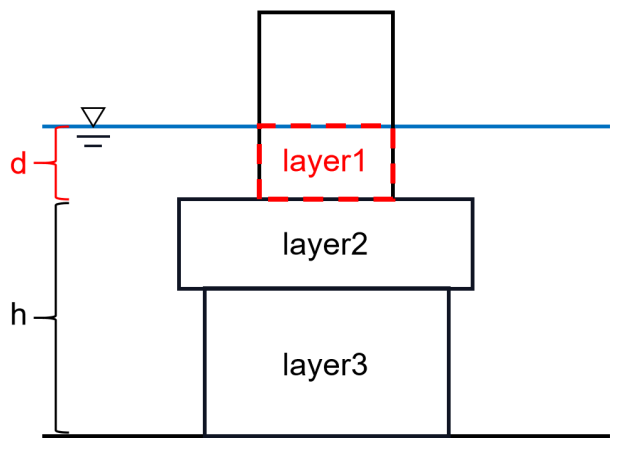
Figure 1Layer schematization for vegetation in SWAN. The submerged part of the plant can be layered by diameter and by the drag coefficient (layer 1, layer 2, layer 3). Each layer has a different thickness, with d for layer 1.
Another important modification of the VEG module concerns the energy dissipation due to wave forces. In the VEG module, the wave force is derived from the drag force in a Morison-type equation with the inertial forces neglected. Since the vegetation is assumed to be a cylinder with a small diameter, the drag force is considered to be dominant. However, for the floating offshore wind turbine, the diameter of the cylinder cannot be neglected compared to the wavelength. The wave forces become more complex and require the consideration of inertial forces. The equation for the energy dissipation due to inertial forces (Finer) can be derived from the work of Morison et al. (1950):
where ρ is the fluid density, V is the volume, CM is the inertial force coefficient, b is the cylinder diameter, h+d is the water depth, d is the draft depth (Fig. 1), and u is the horizontal fluid velocity. Following Kobayashi et al. (1993), the fluid convective accelerations and stresses are assumed to be negligible in this region as a first approximation. The linearized horizontal and vertical momentum equations can be expressed as
Equations (2) and (3) are used to express u and w (vertical fluid velocity) in terms of p (the dynamic pressure):
To solve the linearized problem, it is convenient to introduce the complex wave number , where ki is the exponential decay coefficient, and k is the wave number.
The continuity equation is given by
Substituting Eqs. (4) and (5) into Eq. (6) and solving the resulting equation with the conditions w=0 at , p is given by
where , ω is the wave angular frequency, H is the wave height, and ε is the dimensionless damping coefficient.
In the case of weak damping the dimensionless damping coefficient ε and Eq. (7) with and ] can be shown to be approximated as
with
Substitution of the real parts of Eq. (8) into Eq. (2) yields
Substitution of Eqs. (13), (14), and (10) into Eq. (1) yields
In order to simplify the derivation of the equation, and δ=εc4 are substituted into Eq. (15):
Waves can be described by a joint distribution of wave height, period (or frequency), and direction. For simplicity of analysis, it is usually assumed that all wave heights are related to an average peak period and mean direction. The model developed by Mendez and Losada (2004) describes the transformation of the wave height distribution assuming an unmodified Rayleigh distribution, where the average energy dissipation is as follows:
where the terms with subscript p are associated with the peak period (the subscript p is neglected in the following), p(H) is the Rayleigh probability density function, and Hrms is the root mean square wave height. Substitution of Eq. (18) into Eq. (17) and dividing by the bulk density of the fluid yield
The root mean square wave height and the total wave energy have the relationship , and substituting it into Eq. (19) yields
Equation (20) is the equation calculating the energy dissipation due to the inertial force. In the study, the magnitudes of the inertial force and the drag force are calculated and compared for the cylinders with diameters of 10 and 1 m.
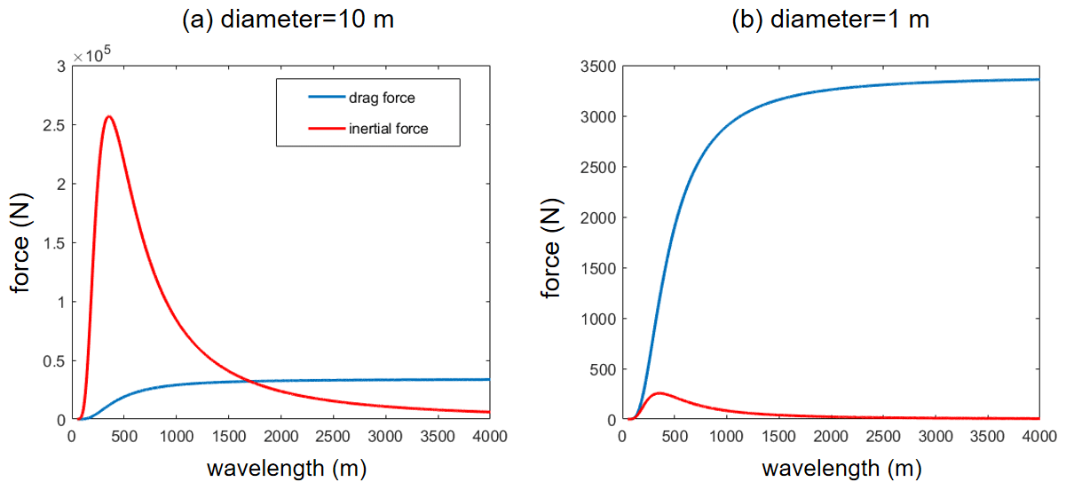
Figure 2Inertial forces (solid red line) and drag forces (solid blue line) for cylindrical diameters of (a) 10 m and (b) 1 m (incident wave height of 3 m, drag coefficient of 1.2, draft depth of 20 m, water depth of 80 m).
The case is set with an incident SWH of 3 m, a drag coefficient of 1.2, a draft depth of 20 m, and a water depth of 80 m. When the cylinder diameter is 10 m (Fig. 2a), the average wavelength of the incident wave is within 1700 m, which makes the inertial force larger than the drag force. However, when the cylinder diameter is 1 m (Fig. 2b), the inertial force is always smaller than the drag force. As the wavelength increases (the scale becomes smaller), the drag force becomes larger relative to the inertial force, which is consistent with the assumption of the VEG module that the inertial force could be neglected, but the inertial force cannot be ignored for the side column of the floating offshore wind turbine. Therefore, the VEG module in SWAN is modified to include the inertial force to be applicable for the floating wind turbine.
As shown in Sect. 2, the floating offshore wind turbine module is developed for SWAN, and its impact on waves is examined using high-resolution numerical experiments in this section.
The rectangular domain of the idealized high-resolution experiments is shown in Fig. 3, with 100×200 cells, a horizontal resolution corresponding to the column diameter of 10 m, and a water depth of 50 m. The position of the column is at the center of the computational domain. The incident SWH is 3 m; the mean wave period is 12 s, propagating from east to west; and the shape of the spectra is from the JONSWAP spectrum. Because of the small computational domain, the model uses stationary computation which converges after several time steps.
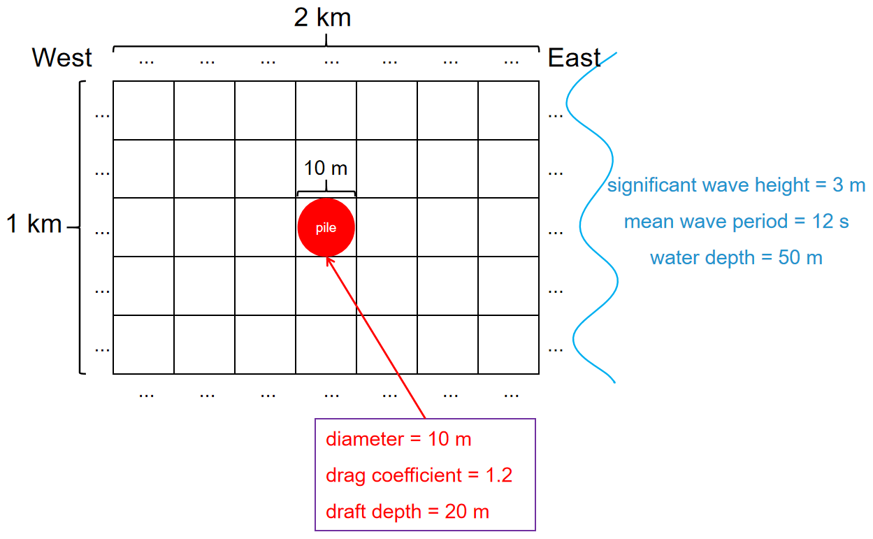
Figure 3Experimental design of high-resolution idealized simulations; the blue curve on the right side represents waves (SWH of 3 m, mean wave period of 12 s, and water depth of 50 m).
Two experiments are conducted, one to study the influence of the column on the waves caused by the drag force only (ExpDragS) and the other to examine the influence caused by both the drag force and the inertial force (ExpInerS). It can be noted that when the energy dissipation is caused by the drag force only, the SWH attenuation is only ∼0.2 m (Fig. 4a), and the “wake” phenomenon occurs in the wave field. The angle of the mean wave direction is shifted by about 1° around the column, and the horizontal distribution is symmetric along the y=0 axis (Fig. 4d). The mean wave length is increased by about 10 m (Fig. 4g). When the inertial forces are taken into account, the energy dissipation is larger, which makes the SWH attenuation more significant, which is about 1.4 m (Fig. 4b), indicating an attenuation of 50 % SWH. The mean wave direction deviation around the column is also relatively large, reaching about 5° (Fig. 4e), and the mean wave length is about 24 m longer (Fig. 4i) than that of ExpDragS.
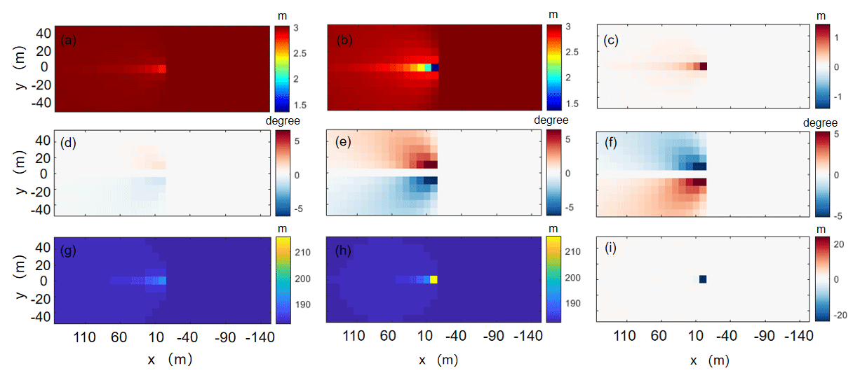
Figure 4Significant wave height of (a) ExpDragS and (b) ExpInerS, (c) difference in significant wave height, (d) mean wave direction deviation of ExpDragS and (e) ExpInerS, (f) difference in mean wave direction deviation, (g) mean wave length of ExpDragS and (h) ExpInerS, and (i) difference in mean wave length.
The results of the idealized high-resolution SWAN simulations in Sect. 3 show the impact of the floating offshore wind turbine's side columns on the waves, including the SWH attenuation; symmetric changes in mean wave direction; and an increase in the mean wave length. However, it is computationally expensive to run a ∼10 m resolution SWAN model.
Using machine learning (ML) to better parameterize unresolved processes in mesoscale and climate models has received much attention in recent years (O'Gorman and Dwyer, 2018; Gettelman et al., 2020; Seifert and Rasp, 2020). With the rise of scientific ML and its widespread use in the geosciences, the design of parameterizations using ML algorithms has become a trend in model development. To build an appropriate model, a large amount of data is needed for training. Nevertheless, observational data on the impact of floating offshore wind turbines on waves are scarce. As a result, the outputs of the high-resolution SWAN simulations in Sect. 3 are employed to train the ML model.
From the equations in Sect. 2, we can note that when the inertial force coefficient, drag force coefficient, and cylindrical diameter are determined, the energy dissipation caused by the wave force is only related to the water depth, incident SWH, and mean wave period (or peak period). We design a series of ideal experiments with different water depths, incident SWH, and mean wave periods. The SWH is taken from 2 to 4 m with a 0.1 m interval. The peak wave period is taken from 7.4 to 7.6 s, 8.4 to 8.6 s, 9.6 to 9.8 s, and 11.0 to 11.2 s with an interval of 0.1 s, and the water depth is selected from 53 to 98 m with an interval of 5 m. This results in a total number of 2520 () experimental groups. We then select simulated data that do not include water depths of 58, 78, and 98 m to train several machine learning (regression) models, since data from these three water depths would be used as validation data. The inputs are incident SWH, water depth, and peak wave period, and the output is SWH after energy dissipation. These models can be classified into four main categories: linear regression models, regression tree models, support vector machines (SVMs), and Gaussian process regression (GPR). These four categories of ML models are described in detail in the Appendix.
As shown in Fig. 5, after training, the GPR model with the Matern 5/2 kernel (covariance) function fits best with a minimum root mean square error (RMSE) of 0.0033 m (Fig. 5d). It may be that the advantage of GPR is mainly in dealing with nonlinear and small sample data. The validation data are also used to analyze the strengths and weaknesses of these four ML models and to prevent overfitting when training the models. Figure 6 shows that the Matern 5/2 GPR model still performs the best, and the stepwise linear regression model still performs the worst. On the other hand, the medium SVM model does not necessarily outperform the fine-tree model in some cases. The ML model can be coupled with CFD, LES models, and mesoscale meteorological models to predict the effect of the floating offshore wind turbine side columns on waves without the need for high-resolution SWAN simulations.
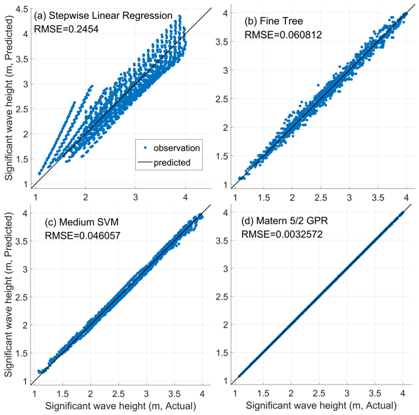
Figure 5Significant wave height scatterplot of the comparison between training data and four typical ML regression models: (a) stepwise linear regression, (b) fine tree, (c) medium SVM, (d) Matern 5/2 GPR.
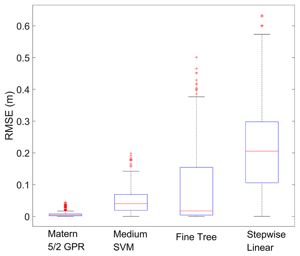
Figure 6Boxplots of RMSE for four typical ML regression models using validation data. The boxplots show the median (horizontal line), 25th to 75th percentiles (box), and 5th to 95th percentiles (whiskers). The whiskers extend to the most extreme data points not considered outliers, and the outliers are plotted individually using the “+” marker symbol.
5.1 Implementation of parameterization in the WRF model
The rate of kinetic energy loss in the grid cell in the original wind farm parameterization scheme (Fitch et al., 2012) is equal to the kinetic energy loss due to the wind turbine in the grid,
where Vijk is the horizontal wind speed, Nij is the number of turbines per square meter, ρ is the air density, CT is the thrust coefficient of a wind turbine, Δx and Δy are the horizontal grid size in the zonal and meridional directions respectively, zk is the height at model level k, and Aijk is the cross-sectional rotor area of one wind turbine bounded by model levels k and k+1 in grid cells i and j.
For a semi-submersible floating wind turbine, the SWH around the turbine is considerably affected. As a result, the roughness of the ocean surface nearby is also changed. This means that the inflow wind speed on the left side of Eq. (21) is no longer the horizontal wind speed in grid cells i and j, and the two must be distinguished:
where Vijk|wt is the recalculated inflow wind speed at the wind turbine site, so a new equation for the momentum tendency term is given as
The corresponding component forms require modification as well:
The tendency of turbulent kinetic energy (TKE) and the power generated by the wind turbine also need to be modified:
where CP is the power coefficient, and CTKE denotes the TKE coefficient calculated by .
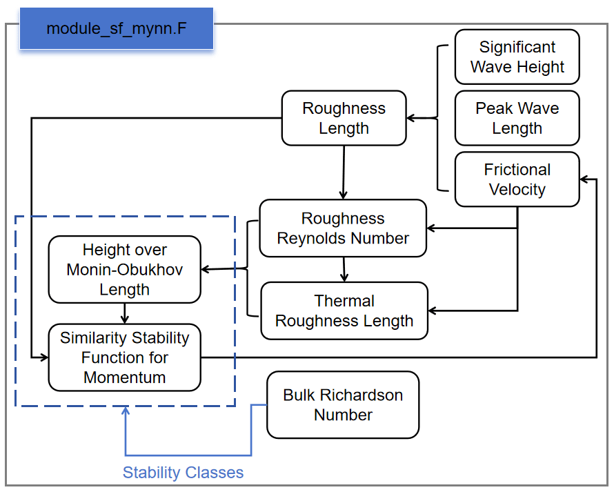
The variables exchanged between WRF and SWAN are shown in Fig. 7. WRF provides 10 m surface wind to SWAN, whereas SWAN returns SWH, peak wave length, and peak wave period to WRF. This variable exchange is implemented in the coupled model. The trained GPR model needs water depth as the input; thus we implement SWAN to provide water depth to WRF. Specifically, we incorporate the GPR model into the surface layer parameterization module of WRF. As a result, the SWH affected by the floating offshore wind turbine can be calculated directly in the surface layer parameterization module to obtain the roughness length, frictional velocity, and other variables. The above variables are then passed to the planetary boundary layer driver module to calculate the three-dimensional wind speed affected by the boundary layer. The three-dimensional wind speed at the wind turbine location is also passed to the new wind farm parameterization.
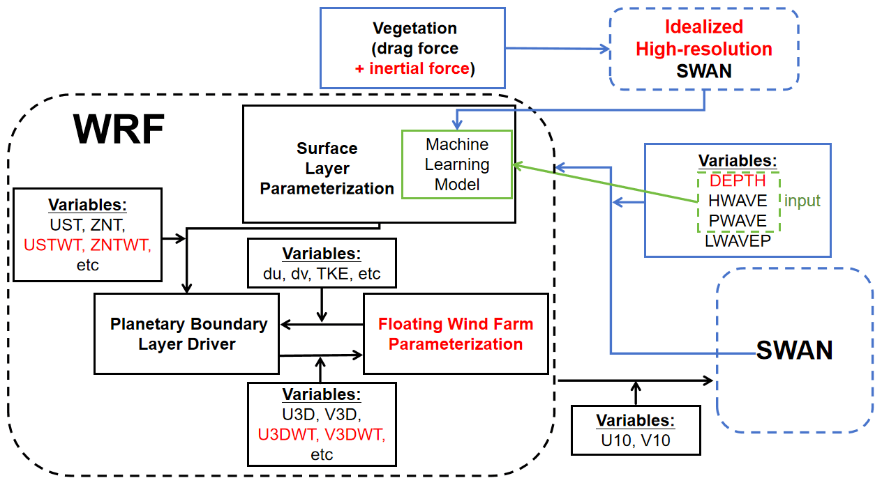
Figure 7Flowchart of floating offshore wind farm parameterization implemented in the coupled model (significant wave height – HWAVE, peak wave period – LWAVEP, peak wave length – PWAVE, water depth – DEPTH, zonal wind at 10 m – U10, meridional wind at 10 m – V10, frictional velocity – UST, frictional velocity at the wind turbine – USTWT, roughness length – ZNT, roughness length at the wind turbine – ZNTWT, three-dimensional zonal winds – U3D, three-dimensional meridional winds – V3D, three-dimensional zonal winds at the wind turbine – U3DWT, three-dimensional meridional winds at the wind turbine – V3DWT, turbulent kinetic energy – TKE, zonal momentum increment – du, meridional momentum increment – dv).
5.2 Model configuration
The model (COAWST; Warner et al., 2010) used to run coupled simulations in this study activates only the atmospheric model (WRFv4.2.2) and the spectral wave model (SWANv41.31).
Initial and lateral boundary conditions for the WRF model are derived from the National Centers for Environmental Prediction Global Data Assimilation System (GDAS) final analysis with a temporal resolution of 6 h and horizontal resolution of 0.25° (NCEP, 2015). The WRF model is configured with 47 vertical levels, where 23 levels are below 1000 m, and 15 levels intersect the rotor region. The vertical spacing of the grid on the levels spanned by the wind turbine rotor is approximately 14 m. The WRF model is configured with two nested domains with a horizontal resolution of 9 and 3 km (Fig. 8a). The outer domain (D01) has 300×220 grids, and the inner domain (D02) has 250×163 grids. The major physical parameterization schemes are summarized in Table 1. The wind farm is located in the northern South China Sea where the water depths range from 50 to 63 m (Fig. 8a). The distance between the turbines is approximately 1 km. The thrust and power coefficients of the LEANWIND 8 MW reference turbine (LW) are presented in Fig. 8b. This floating wind turbine is rated at 8 MW, with a rotor diameter of 164 m, a hub height of 110 m, a cut-in wind speed of 4 m s−1, and a cut-out wind speed of 25 m s−1 (Desmond et al., 2016).
SWAN uses a single domain with 8 km horizontal resolution, which is smaller than the WRF outer domain in this study (Fig. 8a). The corresponding parameterization schemes are shown in Table 1. The spectrum is discretized using 24 logarithmically spaced frequency bins from 0.04 to 1.00 Hz and 36 directional bins with 10° spacing. The boundary conditions are taken from the WaveWatch III (WW3) model (WW3DG, 2019). The nonstationary mode of SWAN is used. The WRF model is coupled with the SWAN model every 10 min. The simulations are integrated first for 12 h without the turbines to reach a steady state and then run for another 6 h for comparison (i.e., from 00:00 UTC on 1 January to 18:00 UTC on 1 January 2019). A reference simulation (control run, referred to as WRF-CTL) is performed without the wind farm. Another simulation (WRF-Fitch) is conducted with the Fitch wind farm parameterization. A third simulation (WRF-FWFP) is performed with the new proposed floating wind farm parameterization.
Table 1Physical parameterization schemes used in the coupled model.
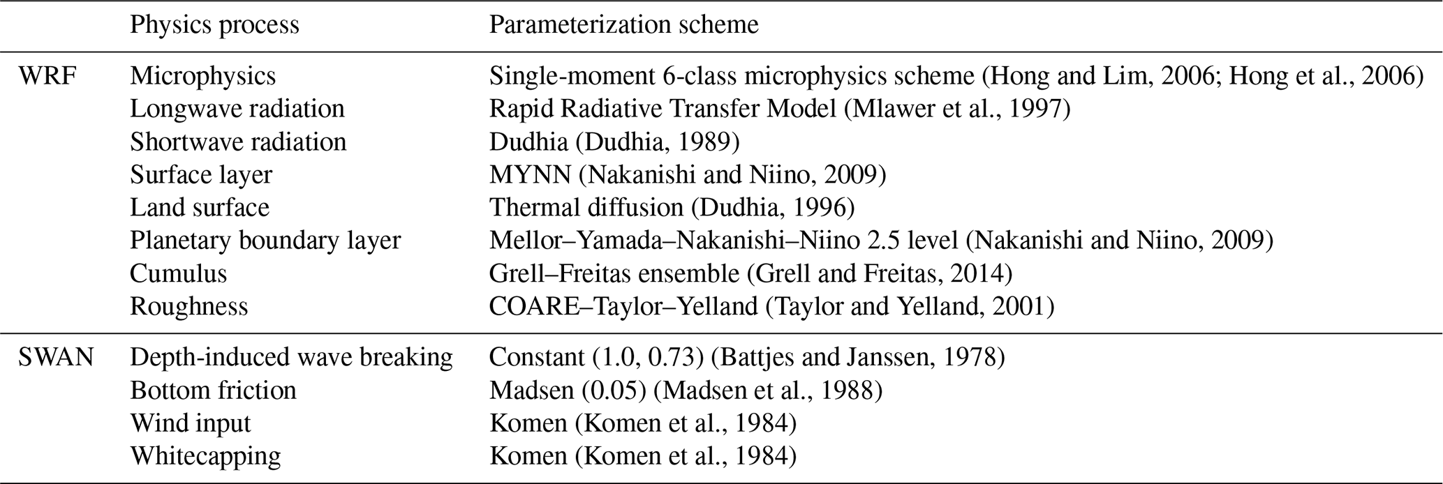
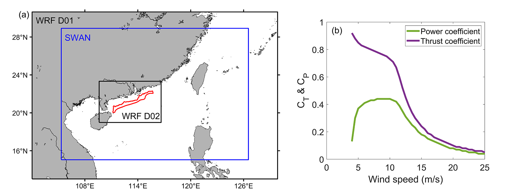
Figure 8(a) The model domain used in COAWST; the solid red line indicates the outer boundary of the wind farm. (b) The thrust and power coefficient curves of the LW 8 MW wind turbine.
5.3 Model validation
To validate the SWAN results, the simulated SWH is compared with observations of the Jason-3 satellite data (Lillibridge, 2019) (Fig. 9). The model is also run for an additional 126 h for further validation (18:00 UTC on 1 January to 00:00 UTC on 7 January). It is evident that the model generally performs well in the wave simulation for the satellite tracks (Pass 38 and Pass 88). The SWH in the model is a bit underestimated on the Pass 12 track and overestimated on the Pass 51 track. Generally, the model results have a reasonable performance.
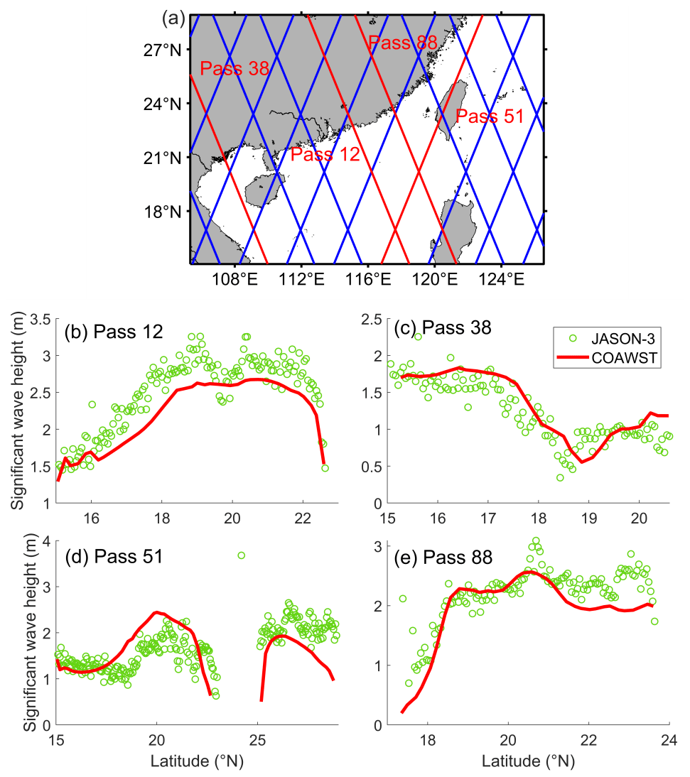
Figure 9(a) Jason-3 ground track in the study area, where the solid red lines representing the tracks are in the period from 00:00 UTC on 1 January to 00:00 UTC on 7 January 2019. SWH comparison between model results and Jason-3 data at (b) 22:00 UTC on 3 January, (c) 22:00 UTC on 4 January, (d) 11:00 UTC on 5 January, and (e) 21:00 UTC on 6 January 2019.
5.4 Simulation results
In this section, the differences in power output, wind speed deficits, and turbulent kinetic energy (TKE) between the FWFP and Fitch schemes are analyzed in a realistic case using the fully coupled atmosphere–wave model. The last 6 h (12:00 UTC on 1 January to 18:00 UTC on 1 January) of simulations are averaged for all results shown below.
5.4.1 Power output and wind speed deficits
For the majority of wind turbines (93.2 % of the number of grids), the power output of WRF-Fitch is smaller than that of WRF-FWFP. This is most likely due to the fact that the FWFP scheme takes into account that the frictional velocity is lower (the inflow wind speed is higher). The difference in power output of a grid cell can reach a maximum of 18 MW (Fig. 10a), which means that the difference in power output of a single turbine can reach a maximum of 2 MW (about nine turbines in a grid cell). In a small area (6.8 % of the number of grids, Fig. 10c), the power output of WRF-Fitch is greater than that of WRF-FWFP, but the difference in power output can only reach a maximum of 0.06 MW (3 %), and most of the positive differences are located in the upstream grid cells (Fig. 10b). On average, the power prediction in the FWFP scheme increases by 12 % compared to the Fitch scheme (Fig. 10d).
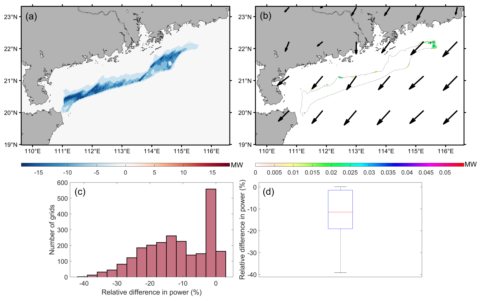
Figure 10(a, b) Power output of the WRF-Fitch case minus the WRF-FWFP case, but only positive values are shown in panel (b). The dashed line indicates the outer boundary of the wind farm, and the black arrow indicates the wind direction. (c) Histogram of the relative difference between the power output of the WRF-Fitch case and the power output of the WRF-FWFP case. (d) Boxplot of the relative difference in the power output, as in Fig. 6.
The maximum value of momentum reduction at hub height for the FWFP scheme is 8 m s−1 (Fig. 12a). Downstream of the wind farm, the wind speed deficit extends into a long wake. The length of the wake reaches 70 km for a wind speed deficit of 1 m s−1 (Fig. 13a). Previous studies have found that roughness lengths and turbulence intensity are lower when the subsurface of the atmosphere is oceanic. Therefore, the wake behind offshore wind farms is expected to be much longer than onshore (∼50 km) (Emeis et al., 2016; Lundquist et al., 2019). The difference in wind speed at hub height between the two schemes has both positive and negative values. The negative values are mainly distributed on the upstream side of the wind farm and in the middle of the wind farm, with a minimum value of about −0.4 m s−1. The positive value areas show a more pronounced difference, up to a maximum of 1.8 m s−1. These effects are also propagated to the wind farm wake (Fig. 12b). The largest uncertainty comes from the surface parameterization scheme in the WRF model. Semi-submersible floating wind turbines weaken the significant wave height, which leads to changes in frictional velocity and roughness length at the wind turbine site. In addition, the atmospheric stability at this location also changes according to the Monin–Obukhov similarity theory (Fig. 11). These factors together lead to a change in the inflow wind speed.
Vertical profiles of wind speed deficits in the WRF-FWFP case also show similar characteristics to the WRF-Fitch case. The atmospheric boundary layer (ABL; including downstream) is affected by the wind speed deficit caused by wind farms (Fig. 13a). A wind speed deficit of 1 m s−1 can extend up to the top of the ABL. Figure 13b shows that the reduction in the momentum of the FWFP scheme also spreads throughout the ABL, which is most pronounced in the rotor area with a maximum value of 1.5 m s−1. The top of the turbine to the top of the ABL and the wind farm wakes also have an effect with values of 0.1 to 0.8 m s−1. The maximum value of the vertical gradient of the wind speed difference is between the hub height and the top of the turbine (163 m).
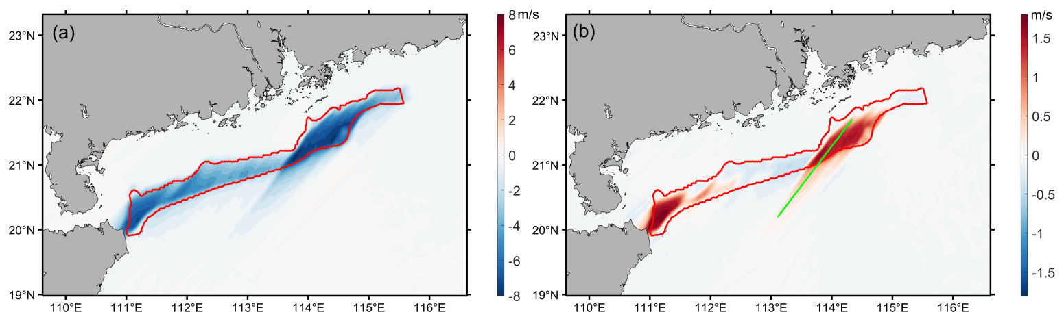
Figure 12Horizontal wind speed of (a) the WRF-FWFP case minus the WRF-CTL case and (b) the WRF-Fitch case minus the WRF-FWFP case at the hub height level. The solid red line indicates the outer boundary of the wind farm, and the solid green line indicates a cross section analyzed further.
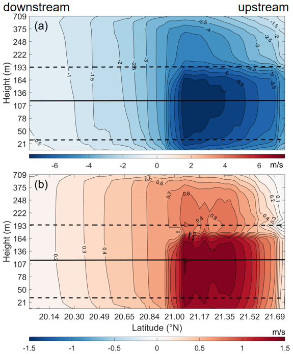
Figure 13Vertical transect of the wind speed of (a) the WRF-FWFP case minus the WRF-CTL case and (b) the WRF-Fitch case minus the WRF-FWFP case along the solid green line in Fig. 12b. The turbine hub height is indicated by the solid horizontal line, and the turbine blade bottom and top are indicated by the dashed lines.
5.4.2 TKE
Despite the advection of TKE, it decays rapidly downstream. TKE generated within the wind farm is largely localized within the wind farm area. The maximum increase in TKE at the top of the turbines within the wind farm is 3.5 m2 s−2 (Fig. 14a). The distribution of horizontal TKE differences is highly similar to that of horizontal wind speed differences (Fig. 12b), indicating that the wind shear may dominate the TKE distribution. The reduction in the TKE caused by the wind farm continues to extend more than 100 km downstream near the surface (Fig. 14c). In contrast, there are two localized areas within the wind farm where the TKE rises obviously, corresponding to the two areas with the greatest increase in TKE at the top of the turbine (Fig. 14c). There is little difference in TKE between WRF-Fitch and WRF-FWFP near the surface downstream (Fig. 14d), with most of the differences occurring only within the wind farm. The distribution of differences in TKE near the ground is almost identical to that at the top of the turbine, except that the value is smaller, by about 0.9 m2 s−2 (60 %), which is most likely due to the vertical transport of TKE. The reduction in TKE near the surface in the downstream (Fig. 14c) is due to a wind speed deficit and corresponding decrease in wind shear in the lower levels of the wake, resulting in a decrease in shear production in TKE, and the reduction in the TKE is not higher than at the top of the turbine (Fitch et al., 2012).
As the wind speeds decrease, the increase in TKE extends to the top of the ABL, which is above the wind farm, with an increase of 1 m2 s−2, reaching a height of nearly 709 m (Fig. 15a). At the top of the turbine, the maximum increase in TKE is 3.6 m2 s−2. On the other hand, the TKE below the bottom of the turbine blades decreases more and more as it approaches the sea surface. Figure 14b indicates that the largest effects of the FWFP scheme on the TKE also appear at the top of the turbine (−1.4–0.6 m2 s−2). It is evident that these results are not influenced by advection but by vertical transport, spreading throughout the ABL.
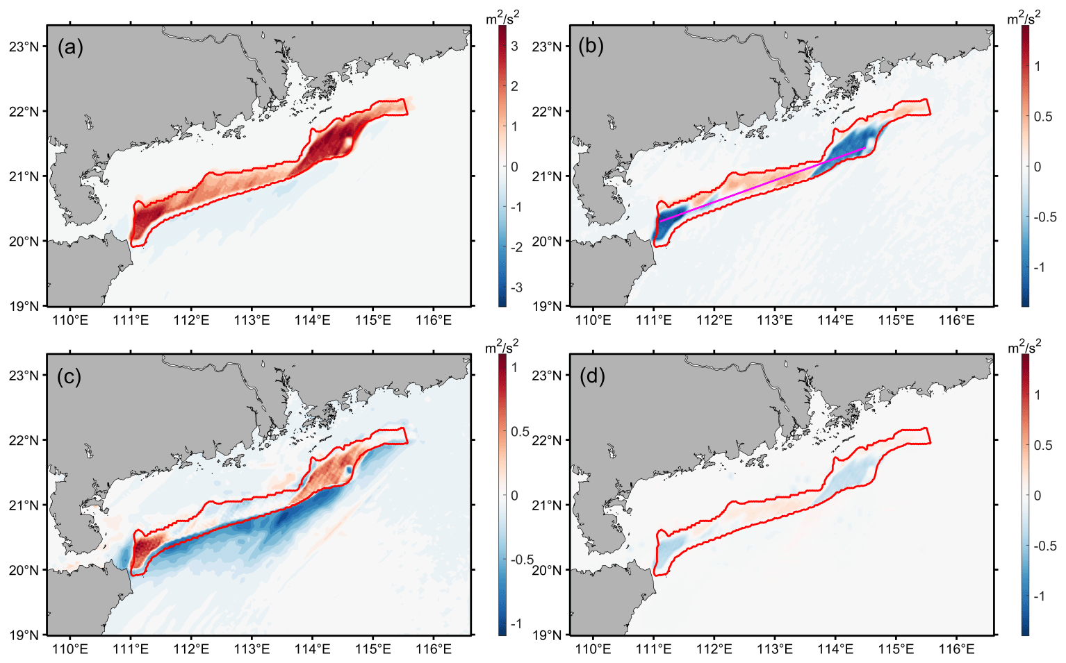
Figure 14Horizontal TKE of (a) the WRF-FWFP case minus the WRF-CTL case and (b) the WRF-Fitch case minus the WRF-FWFP case at the top of the turbine. Horizontal TKE of (c) the WRF-FWFP case minus the WRF-CTL case and (d) the WRF-Fitch case minus the WRF-FWFP case near the sea surface. The solid red line shows the outer boundary of the wind farm, and the solid pink line indicates a cross section analyzed further.
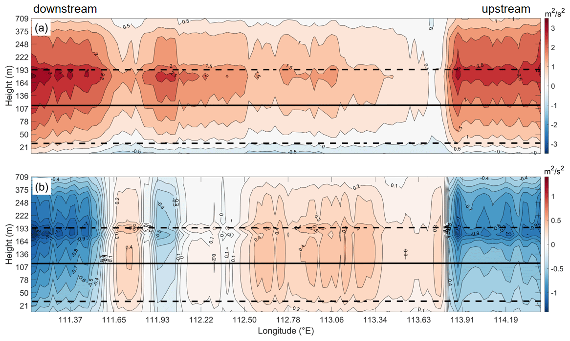
Figure 15Vertical transect of the TKE of (a) the WRF-FWFP case minus the WRF-CTL case and (b) the WRF-Fitch case minus the WRF-FWFP case along the solid pink line in Fig. 14b. The turbine hub height is indicated by the solid horizontal line, and the turbine blade bottom and top are indicated by the dashed lines.
The changes in TKE generation due to the new wind farm parameterization are mainly due to variation in wind shear and vertical transport, which are further analyzed and quantified using the TKE budget. In the planetary boundary layer scheme (MYNN 2.5), the TKE is expressed as
where Ps is the shear production term, Pb is the buoyancy production term, Pv is the vertical transport term, and Pd is the dissipation term. Details about the equations can be found in Janjic (2001).
The largest sources of the difference in TKE between the two cases are shear generation and vertical transport, with the dissipation term almost negligible (Fig. 16). Vertical transport clearly affects the TKE from the bottom of the turbine blade to the sea surface and from the hub height to a height of 248 m. The TKE from above the turbine increases the TKE from the hub height to the top of the turbine due to downward vertical transport (Fig. 16a). The intensification in TKE due to shear generation appears at the top of the turbine, while the reduction appears below the top of the turbine (150 to 194 m) (Fig. 16b). In addition, the impacts of shear generation and vertical transport on the TKE in the rotor region are almost exactly opposite, but the effect of shear generation is slightly larger. This also corresponds well with the distribution of the differences in TKE (Fig. 15b).
Subsequently, the positive and negative areas of the TKE on the cross section are analyzed separately. In the region where the TKE decreases (the wind speed increases), the FWFP scheme results in a greater wind speed deficit, which increases the vertical wind shear in the region from the hub height to the top of the wind turbine, thus increasing the TKE (Fig. 17a). In the region where the difference in TKE is positive (and the difference in wind speed is negative), the result is the opposite (Fig. 17b). And in these regions, the FWFP scheme recovers only a small increase in wind speed, which also results in a limited reduction in TKE.
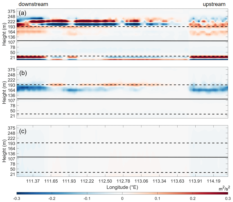
Figure 16Vertical transect of the TKE budget components of the WRF-Fitch case minus the WRF-FWFP case: (a) vertical transport, (b) shear generation, (c) and dissipation along the solid pink line in Fig. 14b. The turbine hub height is indicated by the solid horizontal line, and the turbine blade bottom and top are indicated by the dashed lines.
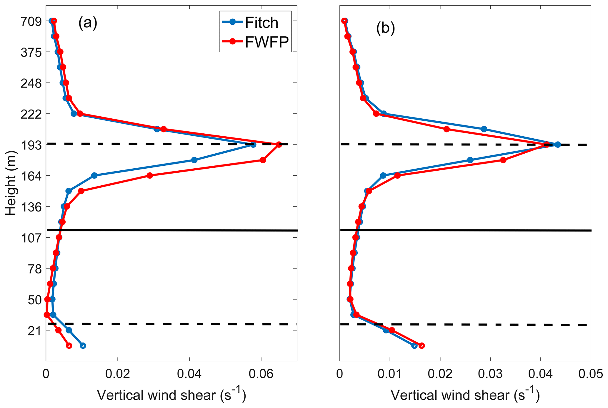
Figure 17Profile of the vertical wind shear along the solid pink line (within the wind farm) in Fig. 14b. (a) Areas where the difference (the WRF-Fitch case minus the WRF-FWFP case) in TKE is negative; (b) areas where the difference (the WRF-Fitch case minus the WRF-FWFP case) in TKE is positive. The turbine hub height is indicated by the solid horizontal line, and the turbine blade bottom and top are indicated by the dashed lines.
Floating wind turbines are essential as the offshore wind industry moves into deeper-ocean regions. However, current wind farm parameterizations can only be applied to fixed turbines. In this study, we develop a floating wind farm parameterization (FWFP) in a coupled model.
Parameters of the column are modified in the VEG module of SWAN to include the effect of the inertial force to make it suitable for the application of the side column of a floating offshore wind turbine. At the same time, a series of idealized high-resolution SWAN simulations is conducted to investigate the dissipation of wave energy induced by the side columns of floating turbines. It is found that under certain conditions, the side columns of floating turbines can attenuate more than 50 % of the significant wave height (SWH), and a wave wake phenomenon occurs with a recovery length of ∼1 km. The mean wave direction is also affected, with a symmetric change of about 5° around the side columns, and the mean wave length increases by more than 20 m. The idealized SWAN simulations and theoretical analyses show that the attenuation of the SWH decreases with increasing water depth and is enhanced with increasing peak wave period. A total of 2520 groups of experiments consisting of different incident SWHs, water depths, and peak wave periods are conducted, and the results of these idealized simulations are used to train a Gaussian process regression (GPR) model with the Matern 5/2 kernel. This model can predict the attenuated SWH due to the side columns of the floating turbine with a given water depth, peak wave period, and incident SWH.
The GPR model is implemented in the surface parameterization module of the WRF to calculate the frictional velocity, roughness length, and other relevant variables at the wind turbine site. These variables are then passed to the planetary boundary layer driver module to calculate the new inflow wind speeds for the Fitch wind farm parameterization to form the FWFP. The difference in the results between the original Fitch scheme and our new FWFP scheme is analyzed in a realistic simulation using a coupled atmosphere–wave model. The results indicate that the FWFP scheme results in higher power output for most of the grid cells in the wind farm (93.2 %) compared to the Fitch scheme, with an average of 12 % higher. This is most likely due to the fact that floating wind farms weaken the SWH and also reduce the roughness length and frictional velocity, which ultimately leads to an increase in the inflow wind speed. There is also a significant difference in the wind speed deficit caused by the two schemes. As a result of the FWFP modification of the inflow wind speed, the wind speed in the upstream region increases (<0.4 m s−1) compared to the Fitch scheme. Wind speeds in the downstream region are reduced, but to a greater extent, to within 1.8 m s−1. The distribution of the differences in TKE corresponds well to the distribution of the differences in wind speed. Compared to the Fitch scheme, the FWFP scheme generates less TKE in the upstream region (<0.6 m2 s−2) and more TKE in the downstream region (<1.4 m2 s−2). The TKE budget demonstrates that shear generation dominates the difference in TKE between the two schemes in the rotor region. Vertical transport is also an important source of TKE variation, and FWFP reduces TKE transport from above the top of the turbine to the lower levels.
Linear regression models are the simplest and most basic class of supervised learning models in machine learning. Stepwise linear regression is an effective method when there are more independent variables. The idea of stepwise linear regression is to introduce the independent variables one by one, and for each independent variable introduced, F tests are performed one by one. When the originally introduced variable becomes insignificant due to the introduction of the later introduced variable, it is dropped, and the process is repeated until the regression equation contains only significant regression variables.
-
Create a one-way regression equation for each independent variable with the dependent variable.
-
Calculate the test statistic F for the regression coefficients in each regression equation separately and find the maximum value . If , stop filtering; otherwise select in the set of variables, and at this point consider to be x1, and proceed to step (3).
-
Separately, calculate the set of independent variables, (x1x2), (x1x3), …, (x1xm), with the dependent variable to create a binary regression equation. Return to step (2), and process the m−1 regression equations. This iterative process results in the optimal regression equation.
Decision trees are a non-parametric supervised learning method for classification and regression. The goal is to create a model that predicts the value of a target variable by learning simple decision rules derived from data features. Depending on the type of data being processed, decision trees fall into two categories: classification decision trees, which can be used to process discrete data, and regression decision trees, which can be used to process continuous data. In the input space where the training data set is located, binary decision trees are constructed by recursively dividing each region into two sub-regions and determining the output values on each sub-region. Suppose that the input space has been divided into M cells (R1R2RM) and that each cell Rm has a fixed output value cm:
-
Select the optimal cutoff variable j and cutoff point s so that Eq. (B1) is minimized.
-
Divide the region with the selected pair (js), and decide the output value of the response.
-
Repeat steps (1) and (2) for both sub-regions until the condition is satisfied.
-
The input space is divided into M regions (R1R2RM) to generate a decision tree.
Support vector regression (SVR) is a regression algorithm based on the support vector machine (SVM) for solving regression problems. Unlike traditional regression algorithms, the goal of SVR is to minimize the difference between predicted and actual values by constructing a prediction function. In addition, unlike general regression, SVR allows the model to have a certain amount of deviation, and the points within the deviation range are not considered problematic by the model, while the points outside the deviation range are counted as losses.
For SVR, the prediction model is as follows:
The optimization objective function is as follows:
subject to .
To eliminate the influence of possible singular-value data on the performance of the SVR model, a slack variable δ is introduced, and Eq. (C2) is transformed into
subject to ,
Among them, c is the penalty parameter, and the larger the value of c, the less adaptive the SVR regression model; a small value of c will lead to a decrease in the sensitivity of δ, increasing the training error. The penalty parameter c is a balanced compromise between the complexity and the adaptability of the SVR model and has to be set in the application. It can be seen that the original objective function is a quadratic programming problem. To facilitate the solution, the Lagrange function is introduced:
where αi, , βi, and are Lagrange multipliers. The optimization problem (Eq. C4) for the original objective function is transformed into a saddle-point problem to solve the Lagrange function:
subject to , αi≥, .
The corresponding regression estimation function is obtained.
In practice, it is often difficult to define feature mappings, which is why kernel functions K(xixj) are introduced.
Gaussian process regression (GPR) is a non-parametric model for regression analysis of data using a Gaussian process prior. GPR is usually used for low-dimensional and small-sample regression problems. In regression prediction, it usually predicts the value of a single point, but GPR can be interpreted as probabilistic prediction, which can predict the exact point as well as the upper and lower bounds, adding more reference value to the prediction. The model assumptions of GPR consist of two parts: the noise (regression residuals) and the Gaussian process prior, and its solution is based on Bayesian inference. The GPR can be expressed as
where μ(x) denotes the mean function, and k(xixj) denotes the kernel (covariance) function, showing that determining the mean and covariance functions is sufficient to determine a GPR. Kernel functions are at the core of GPR, and there are many different kernel functions. For example, the Matern 5/2 covariance function is defined as
where . The kernel parameters are based on the signal standard deviation σf and the characteristic length scale σl.
The given discrete data are (xoyo). Suppose yo and f(x) have a joint Gaussian distribution. The joint probability density formula is then
where Kff=k(xx), Kfy=k(xxo), and Kyy=k(xoxo).
The mean of the prediction is then
The NCEP FNL data (NECP, 2015) can be download from https://rda.ucar.edu/datasets/ds083.3/, wave data (WW3) can be download from https://www.ncei.noaa.gov/thredds-ocean/catalog/ncep/nww3/catalog.html (WW3DG, 2019), and the satellite data (Jason-3) can be obtained from https://www.ncei.noaa.gov/products/jason-satellite-products (Lillibridge, 2019). The coupled model is freely available online (https://github.com/DOI-USGS/COAWST, Warner et al., 2010). Fortran files related to the offshore wind farm parameterization are available in a public repository (https://doi.org/10.5281/zenodo.12180181, Deng, 2024).
SD: methodology, formal analysis, investigation, writing (original draft as well as review and editing); SY: formal analysis, writing (review and editing); SCh: conceptualization, funding acquisition, formal analysis, investigation, writing (review and editing); DC: funding acquisition, writing (review and editing); XY: data curation, investigation; SCu: investigation, writing (review and editing).
The contact author has declared that none of the authors has any competing interests.
Publisher's note: Copernicus Publications remains neutral with regard to jurisdictional claims made in the text, published maps, institutional affiliations, or any other geographical representation in this paper. While Copernicus Publications makes every effort to include appropriate place names, the final responsibility lies with the authors.
The authors would like to thank the two anonymous reviewers for their helpful review comments.
This research has been supported by the Shenzhen Science and Technology Innovation Commission (grant no. WDZC20200819105831001) and the Guangdong Basic and Applied Basic Research Foundation (grant no. 2022B1515130006).
This paper was edited by Nicola Bodini and reviewed by two anonymous referees.
Abkar, M. and Porté-Agel, F.: A new wind-farm parameterization for large-scale atmospheric models, J. Renew. Sustain. Energ., 7, 013121, https://doi.org/10.1063/1.4907600, 2015.
Alari, V. and Raudsepp, U.: Simulation of wave damping near coast due to offshore wind farms, J. Coast. Res., 279, 143–148, https://doi.org/10.2112/JCOASTRES-D-10-00054.1, 2012.
AlSam, A., Szasz, R., and Revstedt, J.: The influence of sea waves on offshore wind turbine aerodynamics, J. Energ. Resour. Technol., Transactions of the ASME, 137, 1–10, https://doi.org/10.1115/1.4031005, 2015.
Archer, C., Wu, S., Ma, Y., and Jiménez, P.: Two corrections for turbulent kinetic energy generated by wind farms in the WRF model, Mon. Weather Rev., 148, 4823–4835, https://doi.org/10.1175/MWR-D-20-0097.1, 2020.
Battjes, J. and Janssen, J.: Energy loss and set-up due to breaking of random waves, Costal Eng. Proc., 1, 32, https://doi.org/10.9753/icce.v16.32, 1978.
Booij, N., Ris, R., and Holthuijsen, L.: A third-generation wave model for coastal regions: 1. model description and validation, J. Geophys. Res.-Atmos., 104, 7649–7666, https://doi.org/10.1029/98JC02622, 1999.
Carvalho, D., Rocha, A., Santos, C., and Pereira, R.: Wind resource modelling in complex terrain using different mesoscale-microscale coupling techniques, Appl. Energ., 108, 493–504, https://doi.org/10.1016/j.apenergy.2013.03.074, 2013.
Dalrymple, R., Kirby, J., and Hwang, P.: Wave diffraction due to areas of energy dissipation, J. Waterw. Port C, 110, 67–79, https://doi.org/10.1061/(ASCE)0733-950X(1984)110:1(67), 1984.
Deng, S.: A Parameterization Scheme for the Floating Wind Farm, Zenodo [data set], https://doi.org/10.5281/zenodo.12180181, 2024.
Desmond, C., Murphy, J., Blonk, L., and Haans, W.: Description of an 8 MW reference wind turbine, J. Phys. Conf. Ser., 753, 092013, https://doi.org/10.1088/1742-6596/753/9/092013, 2016.
Diaz, H. and Guedes Soares, C.: Review of the current status, technology and future trends of offshore wind farms, Ocean Eng., 209, 107381, https://doi.org/10.1016/j.oceaneng.2020.107381, 2020.
Du, J., Bolanos, R., and Guo Larsen, X.: The use of wave boundary layer model in SWAN, J. Geophys. Res.-Oceans, 122, 42–62, https://doi.org/10.1002/2016JC012104, 2017.
Dudhia, J.: Numerical study of convection observed during the winter monsoon experiment using a mesoscale two-dimensional model, J. Atmos. Sci., 46, 3077–3107, https://doi.org/10.1175/1520-0469(1989)046<3077:NSOCOD>2.0.CO;2, 1989.
Dudhia, J.: A multi-layer soil temperature model for MM5, Sixth PSU/NCAR Mesoscale Model Users Workshop 1996, Boulder, CO, PSU/NCAR, 4950, 1996.
Emeis, S.: A simple analytical wind park model considering atmospheric stability, Wind Energy, 13, 459–469, https://doi.org/10.1002/we.367, 2010.
Emeis, S., Siedersleben, S., Lampert, A., Platis, A., Bange, J., Djath, B., Schulz-Stellenfleth, J., and Neumann, T.: Exploring the wakes of large offshore wind farms, J. Phys. Conf. Ser., 753, 092014, https://doi.org/10.1088/1742-6596/753/9/092014, 2016.
Fitch, A.: Climate impacts of large-scale wind farms as parameterized in a global climate model, J. Climate, 28, 6160–6180, https://doi.org/10.1175/JCLI-D-14-00245.1, 2015.
Fitch, A., Olson, J., Lundquist, J., Dudhia, J., Gupta, A., Michalakes, J., and Barstad, I.: Local and mesoscale impacts of wind farms as parameterized in a mesoscale NWP Model, Mon. Weather Rev., 140, 3017–3038, https://doi.org/10.1175/MWR-D-11-00352.1, 2012.
Fitch, A., Olson, J., and Lundquist, J.: Parameterization of wind farms in climate models, J. Climate, 26, 6439–6458, https://doi.org/10.1175/JCLI-D-12-00376.1, 2013.
Gettelman, A., Gagne, D., Chen, C., Christensen, M., Lebo, Z., Morrison, H., and Gantos, G.: Machine learning the warm rain process, J. Adv. Model. Earth Sy., 13, e2020MS002268, https://doi.org/10.1029/2020MS002268, 2020.
Grell, G. A. and Freitas, S. R.: A scale and aerosol aware stochastic convective parameterization for weather and air quality modeling, Atmos. Chem. Phys., 14, 5233–5250, https://doi.org/10.5194/acp-14-5233-2014, 2014.
Hong, S. and Lim, J.: WRF single-moment 6-class microphysics scheme (WSM6), J. Korean Meteorol. Soc., 42, 129–151 ,2006.
Hong, S., Noh, Y., and Dudhia, J.: A new vertical diffusion package with an explicit treatment of entrainment processes, Mon. Weather Rev., 134, 2318–2341, https://doi.org/10.1175/MWR3199.1, 2006.
Isaacson, M.: Wave-induced forces in the diffraction regime, in: Mechanics of wave-induced forces on cylinders, edited by: Shwa, T. L., Pitman Publishing, London, 68–89, 1979.
Janjic, Z.: Nonsingular implementation of the Mellor-Yamada level 2.5 scheme in the NCEP Meso model, NCEP Office note #437 2001, 61, 2001.
Jenkins, A., Paskyabi, M., Fer, I., Gupta, A., and Adakudlu, M.: Modelling the effect of ocean waves on the atmospheric and ocean boundary layers, Energ. Proced., 24, 166–175, https://doi.org/10.1016/j.egypro.2012.06.098, 2012.
Kalvig, S., Manger, E., Hjertager, B., and Jakobsen, J.: Wave influenced wind and the effect on offshore wind turbine performance, Energ. Proced., 53, 202–213, https://doi.org/10.1016/j.egypro.2014.07.229, 2014.
Kobayashi, N., Raichle, A., and Asano, T.: Wave attenuation by vegetation. J. Waterw. Port C., 119, 30–48, https://doi.org/10.1061/(ASCE)0733-950X(1993)119:1(30), 1993.
Komen, G., Hasselmann, S., and Hasselmann, K.: On the existence of a fully developed wind-sea spectrum, J. Phys. Oceanogr., 14, 1271–1285, https://doi.org/10.1175/1520-0485(1984)014<1271:OTEOAF>2.0.CO;2, 1984.
Lillibridge, J.: US DOC/NOAA/NESDIS > Office of Satellite Data Processing and Distribution, Jason-3 Level-2 Operational, Interim and Final Geophysical Data Records (X-GDR), 2016 to present (NCEI Accession 0122595), NOAA National Centers for Environmental Information [data set], https://www.ncei.noaa.gov/archive/accession/0122595 (last access: 25 January 2024), 2019.
Lundquist, J., DuVivier, K., Kaffine, D., and Tomaszewski, J.: Costs and consequences of wind turbine wake effects arising from uncoordinated wind energy development, Nature Energy, 4, 26–34, https://doi.org/10.1038/s41560-018-0281-2, 2019.
Ma, Y., Archer, C., and Vasel-Be-Hagh, A.: Comparison of individual versus ensemble wind farm parameterizations inclusive of sub-grid wakes for the WRF model, Wind Energy, 25, 1573–1595, https://doi.org/10.1002/we.2758, 2022a.
Ma, Y., Archer, C. L., and Vasel-Be-Hagh, A.: The Jensen wind farm parameterization, Wind Energ. Sci., 7, 2407–2431, https://doi.org/10.5194/wes-7-2407-2022, 2022b.
Madsen, O., Poon, Y., and Graber, H.: Spectral wave attenuation by bottom friction: Theory, Proceedings of the 21st International Conference Coastal Engineering, 492–504, 1988.
McCombs, M., Mulligan, R., and Boegman, L.: Offshore wind farm impacts on surface waves and circulation in Eastern Lake Ontario, Coastal Eng., 93, 32–38, https://doi.org/10.1016/j.coastaleng.2014.08.001, 2014.
Mendez, F. and Losada, I.: An empirical model to estimate the propagation of random breaking and nonbreaking waves over vegetation fields, Coastal Eng., 51, 103–118, https://doi.org/10.1016/j.coastaleng.2003.11.003, 2004.
Mlawer, E., Taubman, S., Brown, P., Iacono, M., and Clough, S.: Radiative transfer for inhomogeneous atmospheres: RRTM, a validated correlated-k model for the longwave, J. Geophys. Res.-Atmos., 102, 16663–16682, https://doi.org/10.1029/97JD00237, 1997.
Molen, J., Smith, H., Lepper, P., Limpenny, S., and Rees, J.: Predicting the large-scale consequence of offshore wind turbine array development on a North Sea ecosystem, Cont. Shelf Res., 85, 60–72, https://doi.org/10.1016/j.csr.2014.05.018, 2014.
Morison, J., Johnson, J., and Schaaf, S.: The force exerted by surface waves on piles, J. Petrol. Technol., 2, 149–154, https://doi.org/10.2118/950149-G, 1950.
Nakanishi, M. and Niino, H.: Development of an improved turbulence closure model for the atmospheric boundary layer, J. Meteorol. Soc. Jpn. Ser., 87, 895–912, https://doi.org/10.2151/jmsj.87.895, 2009.
National Centers for Environmental Prediction/National Weather Service/NOAA/U.S. Department of Commerce (NCEP): NCEP GDAS/FNL 0.25 Degree Global Tropospheric Analyses and Forecast Grids, Research Data Archive at the National Center for Atmospheric Research, Computational and Information Systems Laboratory [data set], https://rda.ucar.edu/datasets/ds083.3/ (last access: 20 June 2024), 2015.
O'Gorman, P. and Dwyer, J.: Using machine learning to parameterize moist convection: Potential for modeling of climate, climate change, and extreme events, J. Adv. Model. Earth Syst., 10, 2548–2563, https://doi.org/10.1029/2018MS001351, 2018.
Pan, Y. and Archer, C.: A hybrid wind-farm parametrization for mesoscale and climate models, Bound.-Lay. Meteorol., 168, 469–495, https://doi.org/10.1007/s10546-018-0351-9, 2018.
Paskyabi, M., Zieger, S., Jenkins, A., Babanin, A., and Chalikov, D.: Sea surface gravity wave-wind interaction in the marine atmospheric boundary layer, Energ. Proced., 53, 184–192, https://doi.org/10.1016/j.egypro.2014.07.227, 2014.
Ponce de León, S., Bettencourt, J., and Kjerstad, N.: Simulation of irregular waves in an offshore wind farm with a spectral wave model, Cont. Shelf Res., 31, 1541–1557, https://doi.org/10.1016/j.csr.2011.07.003, 2011.
Porchetta, S., Munoz-Esparza, D., Munters, W., Beeck, J., and Lipzig, N.: Impact of ocean waves on offshore wind farm power production, Renew. Energy, 180, 1179–1193, https://doi.org/10.1016/j.renene.2021.08.111, 2021.
Pryor, S., Barthelmie, R., Bukovsky, M., Ruby Leung, L., and Sakaguchi, K.: Climate change impacts on wind power generation, Nat. Rev. Earth Environ., 1, 1–17, https://doi.org/10.1038/s43017-020-0101-7, 2020.
Redfern, S., Olson, J., Lundquist, J., and Clack, C.: Incorporation of the rotor-equivalent wind speed into the weather research and forecasting model's wind farm parameterization, Mon. Weather Rev., 147, 1029–1046, https://doi.org/10.1175/MWR-D-18-0194.1, 2019.
Roddier, D., Cermelli, C., Aubault, A., and Weinstein, A.: Wind Float: A floating foundation for offshore wind turbines, J. Renew. Sustain. Energ., 2, 033104, https://doi.org/10.1063/1.3435339, 2010.
Santoni, C., García-Cartagena, E., Ciri, U., Iungo, V., and Leonardi, S.: Coupling of mesoscale Weather Research and Forecasting model to a high fidelity Large Eddy Simulation, J. Phys. Conf. Ser., 1037, 062010, https://doi.org/10.1088/1742-6596/1037/6/062010, 2018.
Seifert, A. and Rasp, S.: Potential and limitations of machine learning for modeling warm-rain cloud microphysical processes, J. Adv. Model. Earth Sy., 12, e2020MS002301, https://doi.org/10.1029/2020MS002301, 2020.
Taylor, P. and Yelland, M.: The dependence of sea surface roughness on the height and steepness of the waves, J. Phys. Oceanogr., 31, 572–590, https://doi.org/10.1175/1520-0485(2001)031<0572:TDOSSR>2.0.CO;2, 2001.
Temel, O., Brictexu, L., and Beeck, J.: Coupled WRF-OpenFOAM study of wind flow over complex terrain, J. Wind Eng. Ind. Aerodyn., 174, 152–169, https://doi.org/10.1016/j.jweia.2018.01.002, 2018.
Vanderwende, B. and Lundquist, J.: Could crop height affect the wind resource at agriculturally productive wind farm sites?, Bound.-Lay. Meteorol., 158, 409–428, https://doi.org/10.1007/s10546-015-0102-0, 2016.
Volker, P. J. H., Badger, J., Hahmann, A. N., and Ott, S.: The Explicit Wake Parametrisation V1.0: a wind farm parametrisation in the mesoscale model WRF, Geosci. Model Dev., 8, 3715–3731, https://doi.org/10.5194/gmd-8-3715-2015, 2015.
Warner, J., Armstrong, B., He, R., and Zambon, J.: Development of a coupled ocean-atmosphere-wave-sediment transport (COAWST) modeling system, Ocean Model., 35, 230–244, https://doi.org/10.1016/j.ocemod.2010.07.010, 2010 (code available at: https://github.com/DOI-USGS/COAWST, last access: 20 June 2024).
WW3DG: User manual and system documentation of Wavewatch, (R) version 6.07, NCEI [data set], https://www.ncei.noaa.gov/thredds-ocean/catalog/ncep/nww3/catalog.html (last access: 25 January 2024), 2019.
Wu, L., Shao, M., and Sahlée, E.: Impact of air-wave-sea coupling on the simulation of offshore wind and wave energy potentials, Atmosphere, 11, 327, https://doi.org/10.3390/atmos11040327, 2020.
Yang, D., Meneveau, C., and Shen, L.: Effect of downwind swells on offshore wind energy harvesting-A large-eddy simulation study, Renew. Energy, 70, 11–23, https://doi.org/10.1016/j.renene.2014.03.069, 2014.
Zou, Z., Zhao, D., Zhang, J., Li, S., Cheng, Y., Lv, H., and Ma, X.: The influence of swell on the atmospheric boundary layer under nonneutral conditions, J. Phys. Oceanogr., 48, 925–936, https://doi.org/10.1175/JPO-D-17-0195.1, 2018.
- Abstract
- Introduction
- Parameterization of the wave inertial force in SWAN
- Idealized high-resolution simulations
- Machine learning parameterization
- Parameterization in the WRF model
- Conclusions
- Appendix A: Linear regression
- Appendix B: Regression tree
- Appendix C: Support vector machines
- Appendix D: Gaussian process regression
- Code and data availability
- Author contributions
- Competing interests
- Disclaimer
- Acknowledgements
- Financial support
- Review statement
- References