DELWAVE 1.0: deep learning surrogate model of surface wave climate in the Adriatic Basin

We propose a new point-prediction model, the DEep Learning WAVe Emulating model (DELWAVE), which successfully emulates the behaviour of a numerical surface ocean wave model (Simulating WAves Nearshore, SWAN) at a sparse set of locations, thus enabling numerically cheap large-ensemble prediction over synoptic to climate timescales. DELWAVE was trained on COSMO-CLM (Climate Limited-area Model) and SWAN input data during the period of 1971–1998, tested during 1998–2000, and cross-evaluated over the far-future climate time window of 2071–2100. It is constructed from a convolutional atmospheric encoder block, followed by a temporal collapse block and, finally, a regression block. DELWAVE reproduces SWAN model significant wave heights with a mean absolute error (MAE) of between 5 and 10 cm, mean wave directions with a MAE of 10–25°, and a mean wave period with a MAE of 0.2 s. DELWAVE is able to accurately emulate multi-modal mean wave direction distributions related to dominant wind regimes in the basin. We use wave power analysis from linearised wave theory to explain prediction errors in the long-period limit during southeasterly conditions. We present a storm analysis of DELWAVE, employing threshold-based metrics of precision and recall to show that DELWAVE reaches a very high score (both metrics over 95 %) of storm detection. SWAN and DELWAVE time series are compared to each other in the end-of-century scenario (2071–2100) and compared to the control conditions in the 1971–2000 period. Good agreement between DELWAVE and SWAN is found when considering climatological statistics, with a small (≤ 5 %), though systematic, underestimate of 99th-percentile values. Compared to control climatology over all wind directions, the mismatch between DELWAVE and SWAN is generally small compared to the difference between scenario and control conditions, suggesting that the noise introduced by surrogate modelling is substantially weaker than the climate change signal.

1 Introduction

The multi-decadal characterisation of wave climate is a primary requirement for a number of applications. Coastal erosion, particularly in sandy, low-lying beaches, is largely dominated by wave-induced sediment transport at multiple timescales, with a short-term response at the seasonal or even at the event scale, mainly given by cross-shore fluxes, and a long-term response at the annual to decadal scale resulting from the modulation of long-shore sediment fluxes and their spatial gradients (USACE, 2002). In transitional environments, wave climate can significantly affect morphodynamic processes both directly by locally reworking morphological features such as shoals and salt marshes (Friedrichs, 2011) or indirectly by controlling the potential sediment supply from the open coast (Di Silvio et al., 2010; Tognin et al., 2021). Wave climate is also an important factor controlling the safety and durability of human infrastructures along the coast as well as offshore. Not least, in the framework of an ever-increasing demand for energy availability, particularly from renewable sources, information on wave climate and its variability is crucial for assessing the feasibility and improving the design of wave energy converter facilities (Astariz and Iglesias, 2015).

In recent decades, the progressively deeper understanding of the physical mechanisms underlying wave dynamics, together with an increasing availability of computational power, has contributed to making wave modelling the reference tool for a number of applications at different scales, from short-term forecasting to multi-decadal hindcasting and climate predictions (Cavaleri et al., 2007; Morim et al., 2020). Nonetheless, surface ocean wave modelling in particular is numerically very expensive. This is related to the fact that surface waves typically span deeply subgrid short spatial and temporal scales which are very far from being resolved in most ocean general circulation models (GCMs). Modelling surface waves therefore typically translates to solving evolution equations of the directional wave-energy spectrum, requiring direction and frequency discretisation at each model grid point, thus inflating computational demand. Furthermore, notwithstanding the continuous improvements and particularly when dealing with long-term projections, numerical modelling maintains an intrinsic uncertainty at different levels. This impacts not only the very evolution of the global climate, but also the propagation of the climate signal through different scales and systems and the numerical description and parameterisation of the processes involved. Part of this uncertainty can be addressed by means of an ensemble approach, in which multiple model descriptions are provided by considering different physical characterisations and a different composition of the modelling chain (Parker, 2013). This approach comes at the cost of multiplying, usually by an order of magnitude, the requirements for computational power and data storage. This tends to limit the feasibility of extensive studies on future wave climate, particularly at the regional to local scale, and can require some heavy trade-off in terms of resolution, geographical and temporal coverage, or size of the model ensemble.

Deep learning has been shown to promise great potential for addressing these issues across multiple fields of science, including machine vision and natural language processing, and, more recently, in various subfields of meteorology (Janssens and Hulshoff, 2022; Beucler et al., 2021; Rasp et al., 2018) and oceanography (Rus et al., 2023; Sonnewald et al., 2021; Boehme and Rosso, 2021; Žust et al., 2021; Mallett et al., 2018). With particular reference to wave dynamics applications, James et al. (2018) proposed a machine learning system for predicting the steady-state response of the sea state in a coastal area to a given wind configuration, whereas Rodriguez-Delgado and Bergillos (2021) developed a framework for propagating the open-sea information on incoming waves onshore for renewable energy production purposes. In specific cases and for specific tasks, deep learning methods have been shown to achieve state-of-the-art performance, while keeping numerical costs low. This allows for performance gains, which are often welcome, in particular when considering computational requirements of classical geophysical numerical models at high spatial resolutions and at climate timescales.

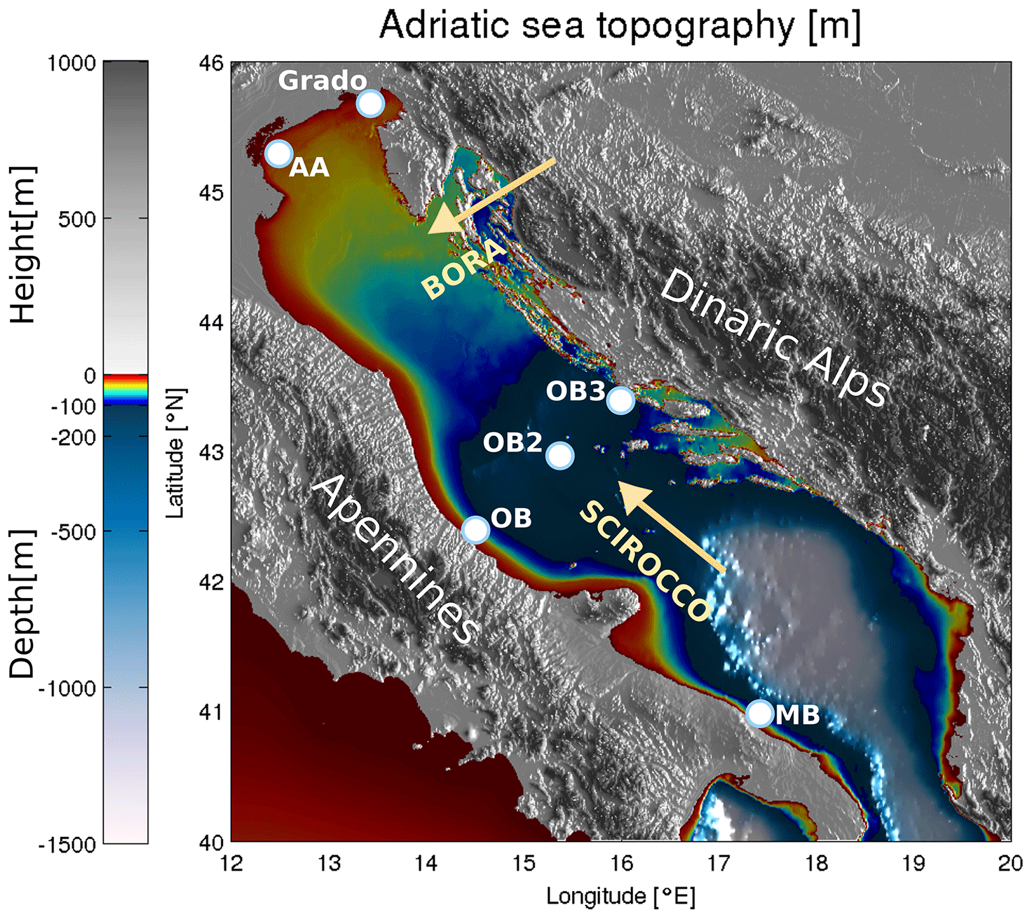
Figure 1 Topography and bathymetry of the Adriatic region. Abbreviations used on the map are as follows: AA stands for Acqua Alta tower, OB (2 and 3) for Ortona buoy (2 and 3), and MB for Monopoli buoy. Directions of Bora and Scirocco are marked with beige arrows. The image was created by the authors based on EMODnet bathymetry data, available at https://portal.emodnet-bathymetry.eu/ (last access: 8 June 2022) and the Copernicus European Digital Elevation Model, available at https://land.copernicus.eu/imagery-in-situ/eu-dem/eu-dem-v1-0-and-derived-products/eu-dem-v1.0 (last access: 8 June 2022).

In this paper, we present a newly developed deep learning method, named the DEep Learning WAVe Emulating model (DELWAVE), for emulating non-stationary modelled surface sea states, such as those produced by the Simulating WAves Nearshore (SWAN) model, albeit at a computational price smaller by several orders of magnitude, in response to given wind fields. The study site is the Adriatic Sea, a 200 km wide and 800 km long elongated epicontinental basin in the north-central Mediterranean. It is surrounded from all sides by the mountain ridges (Apennines in the west, Alps in the north, and Dinaric Alps in the east), which topographically constrain winds over the basin (Fig. 1). From a modelling point of view, this condition requires a high-resolution description of the atmospheric dynamics and a fine tuning of the physical parameterisations both at the air–sea and land–sea interfaces (Cavaleri et al., 2018). Dominant wind–wave forcings consist of the cold northeasterly Bora and warmer southeasterly Scirocco winds. Bora events are predominantly winter occurrences (November through March) of cross-basin continental airflow through the Dinaric orographic barriers over the Adriatic Sea. Scirocco is, on the other hand, a southerly wind that transports warm and moist air masses from northern Africa over the Adriatic, can persist for several days, and is channelled by the Apennines and Dinaric Alps into an along-axis wind, with a fetch much longer than in the case of Bora. Wave dynamics in the Adriatic Sea are thus controlled by short-fetched wind seas and long-fetched swells, which occasionally coexist and propagate over a broad and shallow continental margin, and are characterised by different multi-decadal trends (Pomaro et al., 2018) and possibly different responses to climate change (Bonaldo et al., 2020). As a typical example of some major challenges associated with wave modelling in semi-enclosed and coastal seas, the Adriatic Sea appears to be a suitable testing site for wave model emulation within the DELWAVE framework.

DELWAVE is based on well-established network architecture components, adapted to the field of wave forecasting, and it is benchmarked against SWAN performance, both models forced by the Climate Limited-area Model (COSMO-CLM) atmospheric climate model of the far-future climate (2071–2100) in the Adriatic Basin (Bonaldo et al., 2020).

While DELWAVE model, presented in this paper, has been trained and tested on the outputs of COSMO-CLM and SWAN models, the model can be used with any regional atmospheric and wave modelling setup, or their ensembles, provided that available model results span a large enough time window to make DELWAVE training meaningful.

The paper is organised as follows. Classical geophysical models, COSMO-CLM for atmosphere and SWAN for surface wave modelling, are described in Sect. 2. DELWAVE deep network is thoroughly discussed in Sect. 3. Results and the far-future climate simulations are presented in Sect. 5.

2 Numerical models and datasets

The wind and wave fields used as a reference for this application were retrieved from the numerical modelling chain described by Bonaldo et al. (2020) for the projection of future wave climate in a severe climate change scenario.

2.1 Atmospheric climate model COSMO

The wind fields used for the present applications were retrieved from an implementation of the regional climate model (RCM) COSMO-CLM (Bucchignani et al., 2016), the climate version of the operational forecast model COSMO-LM (Steppeler et al., 2003) implemented over Italy and central Europe at a 0.0715° horizontal resolution (approximately 8 km, totalling 224 × 230 grid points) and forced by the general circulation model (GCM) CMCC-CM (Centro Euro-Mediterraneo sui Cambiamenti Climatici Climate Model; Scoccimarro et al., 2011). In that implementation, the analysed period spanned from 1971 to 2100, reproducing the CMIP5 historical experiment in the 1971–2005 period first and subsequently parting into two independent runs, representing, respectively, the IPCC RCP4.5 (intermediate) and RCP8.5 (severe) scenarios. The evaluation of the model showed particularly good skills in reproducing the climatic features of air temperature and precipitation over Italy (Bucchignani et al., 2016; Zollo et al., 2016). A subsequent focus on the wind fields over the Adriatic Sea (Bonaldo et al., 2017), whose reproduction is a challenging task for hindcast and operational models as well due to the geometry of the basin and its complex coastal orography, highlighted outstanding skills for both intensity, although with some tendency to overestimate mean wind energy and direction. Most interestingly for ocean modelling applications, COSMO-CLM proved capable of capturing the bimodality of Bora (northeasterly) and Scirocco (southeasterly) in the northernmost part of the basin, which would be impossible to reproduce with previous climate models (Bellafiore et al., 2012). In a recent work (Benetazzo et al., 2022) COSMO-CLM was also used to quantile-adjust near-surface wind speeds from the ECMWF ERA5 reanalysis, thus merging the accuracy of the former with the higher temporal resolution and the synchronisation with observed variability in the latter. For the wave modelling experiment described by Bonaldo et al. (2020) and for the present work, the COSMO-CLM wind fields over the Adriatic Sea were retrieved for two 30-year periods in control conditions in the recent past (CTR; 1971–2000) and in the future in a severe RCP8.5 climate scenario (SCE; 2071–2100).

2.2 Wave model SWAN

The modelling run described by Bonaldo et al. (2020) that provides wave data for this application was thus implemented in SWAN, with reference to the Adriatic Sea in the CTR and SCE periods. SWAN provides a phase-averaged description of wind-generated sea states by solving a non-stationary wave action balance equation (Booij et al., 1999):

$$\begin{array}{}\text{(1)}& {\displaystyle \frac{\partial N}{\partial t}}+{\displaystyle \frac{\partial c_{x}N}{\partial x}}+{\displaystyle \frac{\partial c_{y}N}{\partial y}}+{\displaystyle \frac{\partial c_{\mathit{\sigma }}N}{\partial \mathit{\sigma }}}+{\displaystyle \frac{\partial c_{\mathit{\theta }}N}{\partial \mathit{\theta }}}={\displaystyle \frac{S_{\mathrm{w}}}{\mathit{\sigma }}}.\end{array}$$

N represents the action density – namely, the wave energy density divided by the relative frequency – and t is time. The propagation of N (second to fifth term in Eq. 1) is described in 2-dimensional space (x and y, expressible in both Cartesian and spherical coordinates, with speed, represented by c_x and c_y, respectively) and spectral space (radian frequency σ relative to a frame moving with the ocean current; angle θ normal to the wave crest; and speed c_σ and c_θ, respectively). S_w represents sources and sinks of wave energy density associated with generation, dissipation, and non-linear wave–wave interactions.

For the application presented here, the domain was discretised into an orthogonal curvilinear structured grid, with a horizontal resolution ranging from approximately 2 km in the northern region to 8–10 km in the southeasternmost part of the study area. Calm conditions were prescribed at the open boundary at the Otranto Strait, where waves generated within the basin were nonetheless permitted to radiate out of the domain. This assumption was made necessary by the lack of available wave fields consistent with the atmospheric forcing at the Mediterranean scale, but the validation confirmed that no major drawbacks in the results could be found beyond 100–200 km from the boundary. Wave spectra were discretised into 25 logarithmically distributed frequencies, ranging between 0.05 and 0.5 Hz, and 36 directional sectors, whereas the time step was set to 360 s. The bathymetry was reinterpolated from a 1 km resolution dataset used in previous applications (Benetazzo et al., 2014; Bonaldo et al., 2016) and obtained by merging recent surveys in the shallow northern basin and in the southern continental margin into previous basin-scale information. Sea level rise between the CTR and SCE periods was taken into account by increasing the water depth in the latter scenario by 0.70 m, based on estimates by Antonioli et al. (2017), which is, for the sake of simplicity, uniformly distributed throughout the domain. As wind forcings from COSMO-CLM were provided with 6-hourly time step, the same interval was maintained for the output, in which the main spectral parameters were saved for each grid point and the full spectra were saved for approximately 600 points along the Adriatic coast. The model validation was based on directional wave recordings from three observatories off the Italian coast along the main axis of the basin, namely the Acqua Alta oceanographic tower (AA, 45.31° N, 12.51° E; see Pomaro et al., 2018) and the Ortona and Monopoli buoys (respectively, 42.42° N, 14.51° E and 40.98° N, 17.38° E; Fig. 2).

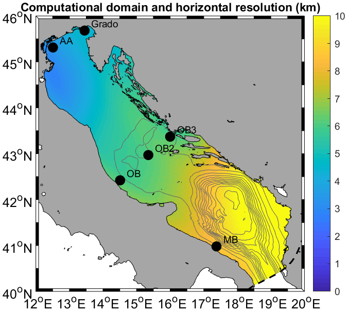
Figure 2 Geographical domain, validation locations, and locations considered in SWAN and DELWAVE modelling.

The comparison to observational data (carried out in statistical terms, as climate models are not synchronised with observed variability) was focused on significant wave height (H_s), and mean direction showed overall satisfactory performances for the SWAN implementation. The reported tendency of COSMO-CLM to overestimate mean wind energy actually had a moderate impact on wave modelling and was partially compensated by other factors such as the southern boundary conditions and some residual limitations in reproducing orographic jets; its more marked effect was a partial overestimate of significant wave height statistics in the southernmost regions of the basin.

The end-of-century projections in a severe climate change condition outlined a composite scenario. While H_s in mean and stormy conditions appeared to decrease in most of the basin and for most directions, the effect of storms from the southern quadrant (southwest to southeast) on the northern Adriatic Sea was expected to intensify. This result, interpreted as a consequence of a northbound shift in the storm tracks (Trenberth et al., 2003; Giorgi and Lionello, 2008) in the Mediterranean region, was shown to have significant implications for the coastal regions. Besides the obvious impact of stronger storms where this will happen and besides the baseline sea level rise exacerbating the effect of storms even when their intensity is expected to decrease (Lionello et al., 2017), the spatial variability in the impact of climate change will result in a modification of the patterns of energy fluxes onto and along the Adriatic coast, thus modifying the sediment transport rates and gradients and, ultimately, coastal morphodynamic processes.

2.3 Training and evaluation datasets

The training and the application of DELWAVE were based on basin-wide wind fields from COSMO-CLM and pointwise wave time series at six locations exposed to different wave climates (Fig. 2), including AA (45.31° N, 12.51° E), OB (42.42° N, 14.51° E), and MB (40.98° N, 17.38° E), which coincide with the observation points used for the SWAN model validation in Bonaldo et al. (2020) and are representative of nearshore conditions, respectively, along the northern, central, and southern Italian coasts. Grado (45.68° N, 13.45° E) lies at the edge of the gulf of Trieste in the northernmost end of the Adriatic Sea, facing south, and is partially sheltered by the Istrian peninsula. OB2 (42.97° N, 15.35° E) and OB3 (43.37° N, 16.00° E) are located along an ideal transect off Ortona, respectively, in the middle of the basin and along the Croatian coast. Wind fields are provided as 6-hourly meridional and zonal components, whereas wave data, also 6-hourly, are given in terms of significant wave height (H_s), mean wave direction (d), and energy period ($T_{\mathrm{m}-\mathrm{1},\mathrm{0}}$). The model data from the control (CTR) period (1971–2000) were used for the network training, whereas future scenario (SCE; 2071–2100) data were used as a reference for assessing the network skills, particularly in terms of their capability to capture the features of the climate signal.

3 DELWAVE

In this section, we present our DEep Learning WAVe Emulator (DELWAVE). DELWAVE is constructed from three logically separate parts. We proceed by providing an overview of the model input fields. Following that, we describe the DELWAVE architecture in detail and further discuss specific model architecture decisions using ablation studies. Lastly, we provide a description of the training procedure.

3.1 Model input tensor

The data DELWAVE uses to conduct both training and inference are available in the form of a tensor, which contains three logically separate fields: spatial wind field, location encoding, and grid encoding. Each of this parts serves a specific purpose, and we elaborate on each in the following subsections.

3.1.1 Wind field

Let's begin by first defining the input (wind) fields from which core information for surface wave prediction is extracted. Let I^t denote the spatial wind field over the Adriatic Basin at time t. Then,

$$\begin{array}{}\text{(2)}& I^t\in {\mathbb{R}}^{\mathrm{2}\times n_x\times n_y},\text{dim}\left(I^t\right)=[\mathrm{2},n_x,n_y],\end{array}$$

where the first dimension corresponds to either u or v components of the wind vector, while the last two correspond to the zonal (n_x) and meridional (n_y) spatial dimensions of the modelled wind field, which, in our case, are n_x=90 and n_y=89.

3.1.2 Location encoding and grid encoding

We further complement the wind field input tensor I^t by a spatial encoding matrix. The purpose of this matrix is to provide the network with information about the specific location for which we wish to predict surface wave attributes. This approach allows us to easily add new locations into the training procedure by simply defining new spatial encoding matrices without the need for any other modifications to the algorithm or model architecture.

Let L_l denote the location encoding sparse matrix for location l. Then, we have

$$\begin{array}{}\text{(3)}& {\mathbf{L}}_l\in {\mathbb{R}}^{n_x\times n_y},\text{ dim}\left({\mathbf{L}}_l\right)=[n_x,n_y].\end{array}$$

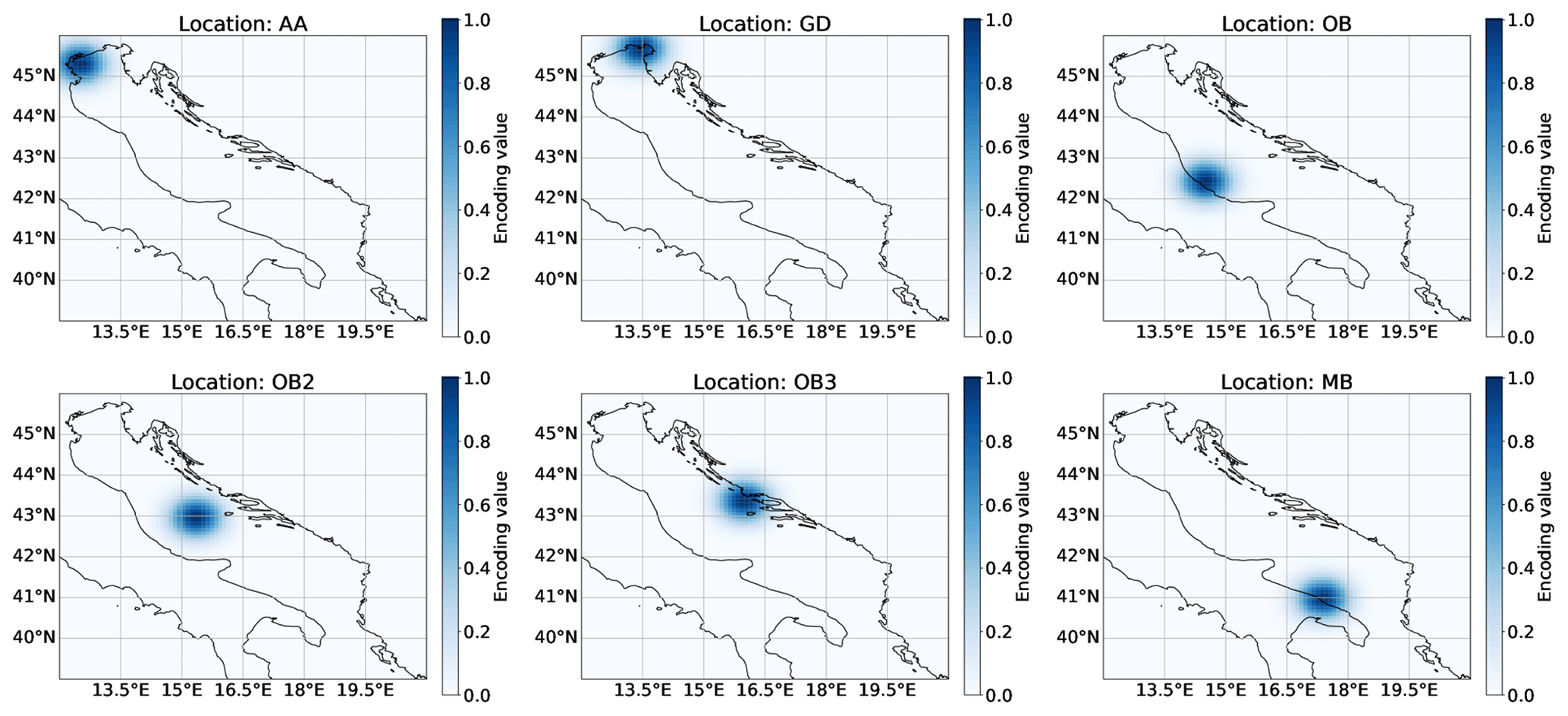
Figure 3 The visualisation of the spatial encoding matrices for each location (the coastline is added for clarity). Each plot corresponds to one location encoding matrix, which forms a part of the input sample tensor, I_l.

We now denote each ith row ($i=\mathrm{1},\mathrm{\dots },n_x$) and jth column ($j=\mathrm{1},\mathrm{\dots },n_y$) entry of L_l as ${\mathbf{L}}_{l,(i,j)}$ and compute the matrix entries as

$$\begin{array}{}\text{(4)}& {\mathbf{L}}_{l,(i,j)}={\displaystyle \frac{\mathrm{1}}{\sqrt{\mathrm{2}\mathit{\pi }}\mathit{\varsigma }}}\exp \left[-{\displaystyle \frac{\mathrm{1}}{\mathrm{2}}}{\displaystyle \frac{(l_i-i+\mathrm{1}{)}^{\mathrm{2}}+(l_j-j+\mathrm{1}{)}^{\mathrm{2}}}{{\mathit{\varsigma }}^{\mathrm{2}}}}\right],\end{array}$$

where we set the spatial variance to ς²=20. This variance corresponds to a standard deviation of $\sqrt{\mathrm{20}}\sim$ 4–5 grid cells or 0.45° in longitude and latitude, as shown in Fig. 3. We determined the value of the spatial variance empirically by testing multiple value configurations where we finally selected the spatial variance value which produced the best results. The variables l_i and l_j denote the corresponding location l's position in the spatial field expressed in terms of row and column indices. We illustrate examples of multiple encodings for different locations in Fig. 3.

Finally, we normalise the matrix entries to the range [0,1] by

$$\begin{array}{}\text{(5)}& {\stackrel{\mathrm{̃}}{\mathbf{L}}}_{l,(i,j)}={\displaystyle \frac{{\mathbf{L}}_{l,(i,j)}-\text{min}\left({\mathbf{L}}_l\right)}{\text{max}\left({\mathbf{L}}_l\right)-\text{min}\left({\mathbf{L}}_l\right)}}.\end{array}$$

We use this normalised location encoding matrix to augment the input wind field tensor to form the wind-location input tensor, $I_l^t$, where the tensor is now given for a specific location target and time.

Here, the augmentation denotes the concatenation of the starting input tensor and the location encoding along the first dimension. This entails that $\text{dim}\left(I_l^t\right)=[\mathrm{3},n_x,n_y]$, where the increased size of the first dimension corresponds to this augmentation. To create training samples for all k locations based on the same wind field, we use the following approach: we first randomly sample a wind field from the dataset. We then augment the wind field with the k location matrices, where each individual augmentation produces its own $I_l^t$ corresponding to a location, l. This way, each training sample contains the wind field together with a spatial encoding of a specific location. As we train the model, the training takes into account all the different locations and all the time steps during the same training process.

This input provides the necessary information for the model to distinguish between the different locations for which we require surface wave predictions. Without this encoding, the model would most likely gravitate towards an average prediction at a specific time, t, for all locations as it would not be able to distinguish between them. During DELWAVE training, we minimise the root mean squared difference loss function, defined as

$$\begin{array}{}\text{(6)}& \mathcal{L}=\sqrt{{\displaystyle \frac{\mathrm{1}}{n}}\sum _{i=\mathrm{1}}^n(y_i-{\widehat{y}}_i{)}^{\mathrm{2}}},\end{array}$$

where y_i denotes the SWAN values for sample i and ${\widehat{y}}_i$ denotes DELWAVE's predictions. If we were to omit the location encoding from the input tensor for time t, then each location would share the same input tensor at time t (the location encoding is what differentiates input tensors for each target location); however, the wave field attributes of each location are not the same. Therefore, the average prediction of all target locations is the minimiser in this case.

The final transformation of the input tensor is the concatenation of the grid encoding. A building block of DELWAVE's architecture is the convolution operation, which is, by design, translation invariant. This implies that the same signal at different spatial locations produces the same output response. Since the location of specific wind patterns in relation to the target location of interest is important (wind fetch), we have to go against this inherent invariability of the convolution operation in translations. We do this using the grid encoding, which assigns a unique value to each spatial location inside the input field. This enables the network to learn wind features in specific regions of the input. We denote the grid encoding matrix as $\mathbf{C}\in {\mathbb{R}}^{n_x\times n_y}$. Individual entries of the matrix are computed as

$$\begin{array}{}\text{(7)}& {\mathbf{C}}_{(i,j)}={\displaystyle \frac{(i-\mathrm{1})n_y+j-\mathrm{1}}{n_x{n}_y}},\end{array}$$

where i is the index of the row and j of the column. We augment the wind-location tensor with the above-defined grid matrix to produce the final wind-location tensor (we do not explicitly denote the grid-encoding presence inside the tensor) in the same way as we did in the case of the location encoding. We end up with a tensor containing four input fields (zonal wind, meridional wind, location encoding, and grid encoding) of dimension [n_x,n_y]:

$$\begin{array}{}\text{(8)}& \text{dim}\left(I_l^t\right)=[\mathrm{4},n_x,n_y].\end{array}$$

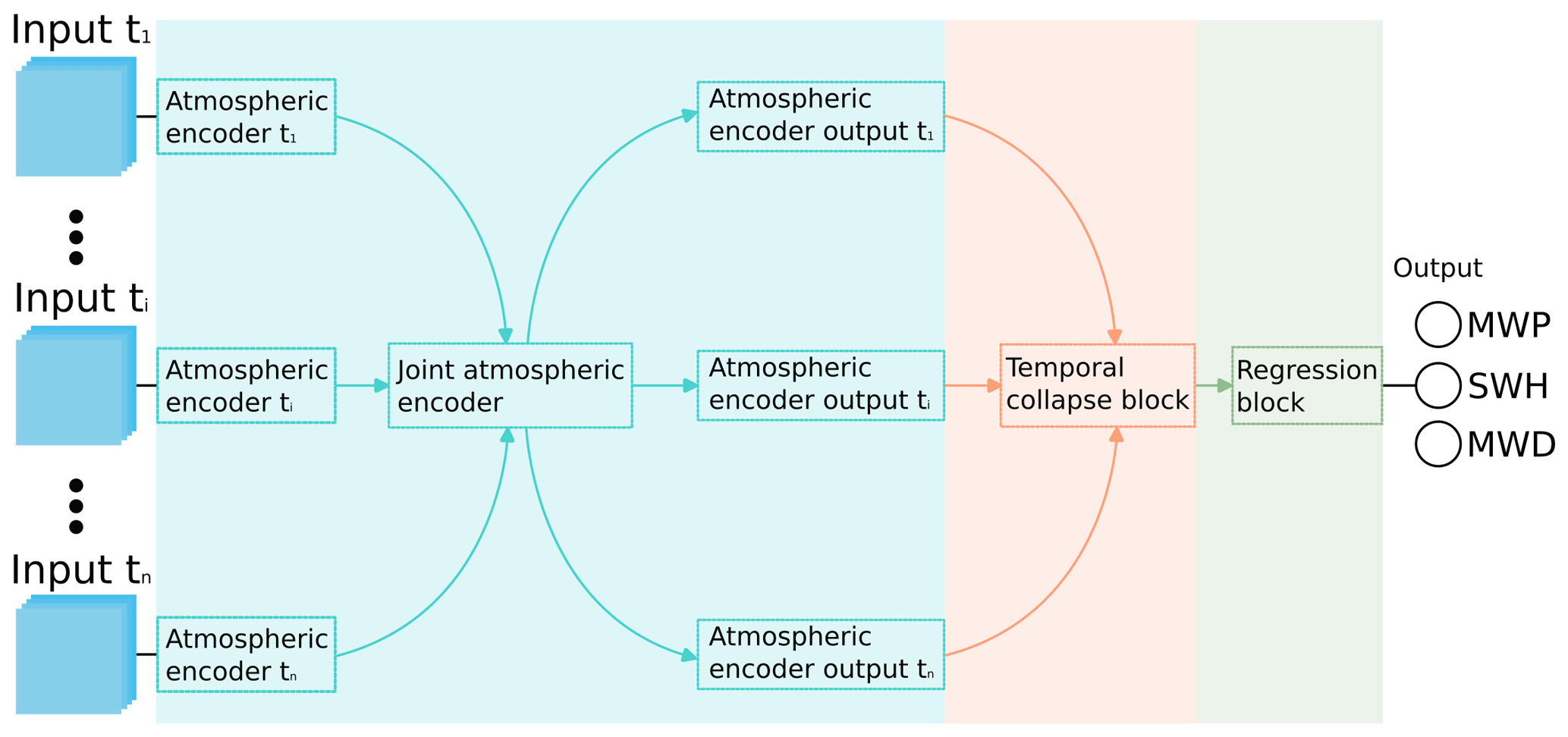
Figure 4 DELWAVE architecture overview. The network is comprised of three logically distinct sections. Each section is denoted using a different colour. The information in the network flows from left to right. Input t_i denotes the n time steps passed on to the network, while MWP, SWD, and MWD denote the mean wave period, significant wave height, and mean wave direction, respectively.

3.1.3 Temporal extent

The surface wave field at a specific location consists of the local wind sea and of the incoming swell, generated remotely in the hours preceding forecast time t. Consequently, predictions at time t require additional wind inputs from times preceding t. The number of preceding time steps was estimated using a deep-water dispersion relation for gravity waves, σ²(k)=gk, and the corresponding gravity wave phase speed:

$$\begin{array}{}\text{(9)}& c_f=\mathit{\sigma }/k=(g/k{)}^{\mathrm{1}/\mathrm{2}}=(g\mathit{\lambda }/\mathrm{2}\mathit{\pi }{)}^{\mathrm{1}/\mathrm{2}}.\end{array}$$

Using an estimate of surface wave wavelength, λ = 40 m, indicates that such waves traverse basin-scale distances in about 1.5 d. We consequently estimate that the wave field at a given location can be influenced by remotely generated swell over distances traversed by swell waves in about 1 to 1.5 d, corresponding to about 10–14 time steps in 3-hourly resolution input. We rounded this down to 10 temporally preceding time steps.

We therefore take 10 preceding wind inputs from consecutive time instants leading up to t – namely $[I_l^{t-\mathrm{10}},I_l^{t-\mathrm{9}},\mathrm{\dots },I_l^{t-\mathrm{1}},I_l^t]$. Repeating this for over four fields contained in the $I_l^t$ tensor (zonal wind, meridional wind, location encoding, and linear grid encoding), we end up with 11 time steps of four fields over a spatial grid of n_x×n_y cells. Hence, the dimensions of final concatenated input tensor are

$$\begin{array}{}\text{(10)}& \text{dim}\left(I_l\right)=[\mathrm{11},\mathrm{4},n_x,n_y]=[\mathrm{11},\mathrm{4},\mathrm{90},\mathrm{89}].\end{array}$$

3.2 DELWAVE model architecture

DELWAVE is composed of three logically distinct components, each responsible for a specific processing task, as depicted in Fig. 4. The atmospheric encoder is responsible for encoding the input fields for each time step into high-dimensional vectors. These vectors are then passed to the temporal collapse block, where they are merged into a single vector and attenuated based on the temporal importance of the individual inputs, as explained in Sect. 3.2.2 below. Finally, the regression block transforms this vector into the three outputs required. Individual blocks are described in more detail in the following subsections.

Additionally, let us define the notion of an encoder. An encoder is a sequence of transformations, a sub-neural network, which maps a specific input to a, usually, high-dimensional vector. This vector is said to be an encoding of the provided input, carrying information about it, albeit in an obtuse way. The encoder–decoder structure Cho et al. (2014), for example, is a common paradigm in machine learning that leverages this terminology.

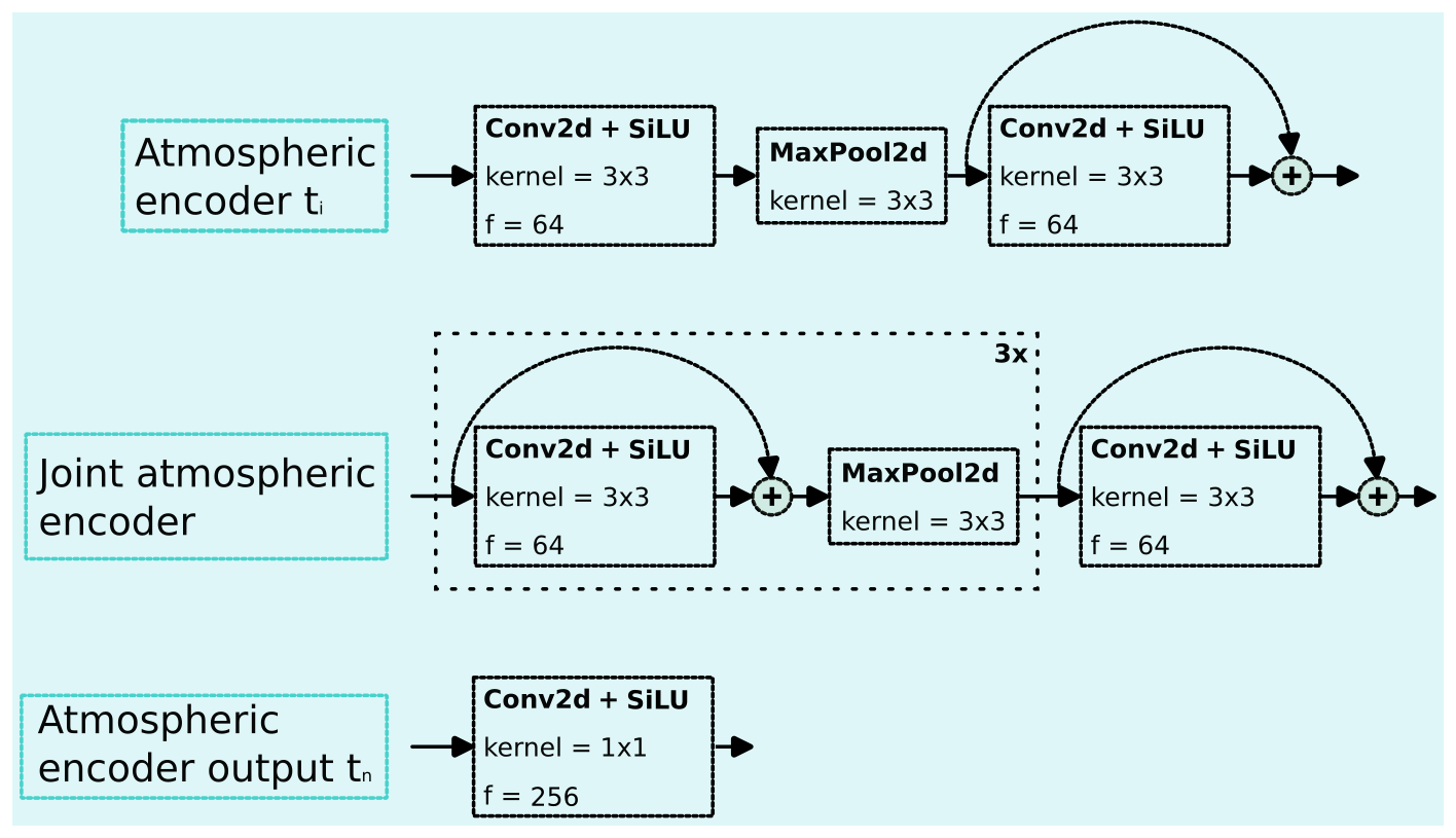
Figure 5 DELWAVE atmospheric encoder block sub-components. Each sub-component is shown in a separate row. The variable f denotes the number of output features of that operation and kernel denotes the kernel size of the convolution operation. Stride is always 1 for the convolution layers and 2 for the maximum pool layers. The activation function of choice is the sigmoid linear unit (SiLU) (Hendrycks and Gimpel, 2016).

3.2.1 Atmospheric encoder block

The atmospheric encoder block, displayed in Fig. 5, is constructed from three sub-components: the per-input atmospheric encoder, the joint atmospheric encoder, and the output atmospheric encoder.

Input atmospheric encoder. The input atmospheric encoder encodes each time step individually before passing them to the joint atmospheric encoder. Each per-time-step input tensor has its own input atmospheric encoder block. This is to ensure that the initial processing of the wind field with the location encoding is unique to each time step. The per-time-step encodings of spatial locations might be important for predicting wave characteristics at different time steps; therefore, per-input encoders add to the flexibility of the model being able to adapt to such requirements. However, using completely separate encoders for each time step would result in slow, hard-to-scale architectures with overfitting issues. Therefore, a shallow initial encoder structure for each time step is a good compromise between the two approaches. Here, shallow denotes an architecture with only a few layers, as is denoted in Fig. 5. Conversely, a deep neural network architecture constitutes of many tens of layers.

To be more formal about the atmospheric encoders, defined as A_j, the jth atmospheric encoder (in our case one of 11), each corresponds to one consecutive time step. Then, DELWAVE proceeds by encoding each time step of the input tensor with its corresponding atmospheric encoder. This results in the following set of atmospherically encoded input tensors:

$$\begin{array}{}\text{(11)}& \mathit{\left\{}{A}_{\mathrm{1}}\right(I_{l,\left(\mathrm{1}\right)}),\mathrm{\dots },A_{\mathrm{11}}(I_{l,\left(\mathrm{11}\right)}\left)\mathit{\right\}},\end{array}$$

where I_l,(j) denotes the jth time step from the input tensor I_l and A_j(I_l,(j)) denotes the encoded tensor. This set is then passed to the next transformation, the joint atmospheric encoder.

Joint atmospheric encoder. The joint atmospheric encoder is the primary extractor of important wind field features as it is also the encoder with the most layers. It is shared between time steps (we use the same joint atmospheric encoder to transform each per-time-step output of the previous block), since we care to locate important wind features independently of the time at which they occurred. For example, a specific wind pattern can occur at different time steps. Therefore, we can use the same wind pattern detector to locate and recognise the pattern irrespective of the time of occurrence. The approach of weight sharing between time steps also reduces the computational complexity and the number of required parameters and acts as a regularising method preventing overfitting. We denote this encoder, which is applied to all output of the individual atmospheric encoders and results in a single output tensor, as A_joint.

$$\begin{array}{}\text{(12)}& A_{\text{joint}}\left(A_{\mathrm{1}}\right(I_{l,\left(\mathrm{1}\right)}),\mathrm{\dots },A_{\mathrm{11}}(I_{l,\left(\mathrm{11}\right)}\left)\right).\end{array}$$

Output atmospheric encoder. The output atmospheric encoder selects the recognised wind features important for each time step. We do this using a convolution operation with a kernel size of 1, signifying a linear combination of the input features. The resulting per-time-step tensors of dimension $[b,\mathrm{256},\mathrm{4},\mathrm{4}]$, where b denotes the batch size, are summed across their last two dimensions, resulting in a 256-dimensional vector as the final output of this layer. These vectors serve as high-dimensional weather descriptors for individual time steps and contain wind information at each time step.

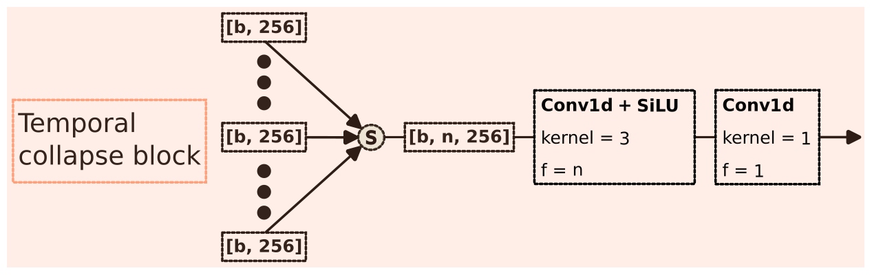
Figure 6 DELWAVE temporal collapse block. The variable n denotes the number of time steps used to train the model, and b denotes the batch size. The n weather feature vectors of dimension [b,256] are stacked to form a single tensor, which is then reduced to a single 256-dimensional vector by passing through the convolutional operations. Stride is always 1 for the convolution layers. The activation function of choice is the sigmoid linear unit (SiLU) (Hendrycks and Gimpel, 2016).

3.2.2 Temporal collapse block

The temporal collapse block, displayed in Fig. 6, collects the individual atmospheric vectors and encodes them into a single 256-dimensional vector. This is done by a sequence of two 1-dimensional convolution operations Conv1d (2024), where we set the kernel size and output feature count to 1 for the latter of the two. This essentially achieves a linear combination of the inputs across the time step dimension. The first convolution produces a new set of interleaved temporal feature vectors. The second block reduces these temporal feature vectors into a single vector by means of a linear combination.

3.2.3 Regression block

Finally, the regression block, displayed in Fig. 7, is comprised of consecutive fully connected layers with skip connections. This block produces the final outputs: MWP, SWH, and MWD. To prevent overfitting and improve performance on unseen data in the test dataset, a dropout with a removal probability of 0.2 is applied prior to each fully connected layer, except for the last one (the output, linear layer).

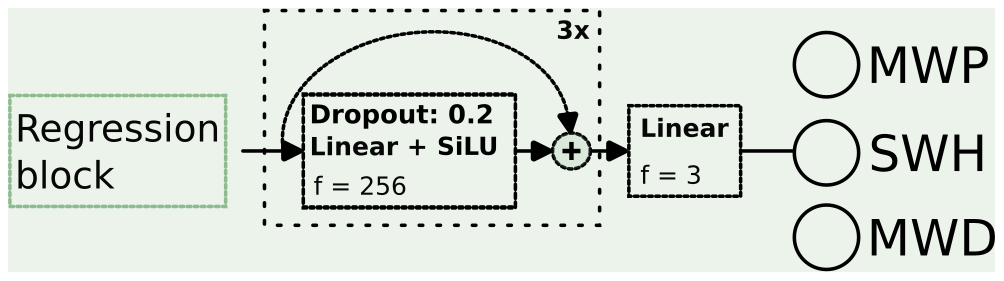
Figure 7 DELWAVE regression block reduces the output of the temporal collapse block into the final outputs: MWP, SWH, and MWD. The regression is conducted by a cascade of three dense skip connections followed by the final dense connection with three outputs. The activation function of choice is the sigmoid linear unit (SiLU) (Hendrycks and Gimpel, 2016).

3.3 Training protocol

The CTR period was used for training, while the SCE period was used for testing the final, developed model. The CTR data were further split into two parts: the actual training dataset (CTR_trn) and the validation dataset (CTR_vld). CTR_trn contains the first 80 % of the training data, while CTR_vld contains the remaining 20 %. The data for each location and for each variable (significant wave height, mean wave period, mean wave direction) are separately standardised to exhibit zero mean and a variance of 1. Prior to the standardisation, we log-transform significant wave heights as ln (SWH+1). We give arguments for this transformation in the following paragraphs. Then, at each training iteration, a random batch of training samples is collected and the model loss function, the root mean squared difference, defined in Eq. (6), is used to optimise DELWAVE's parameters, which are evaluated at these batches.

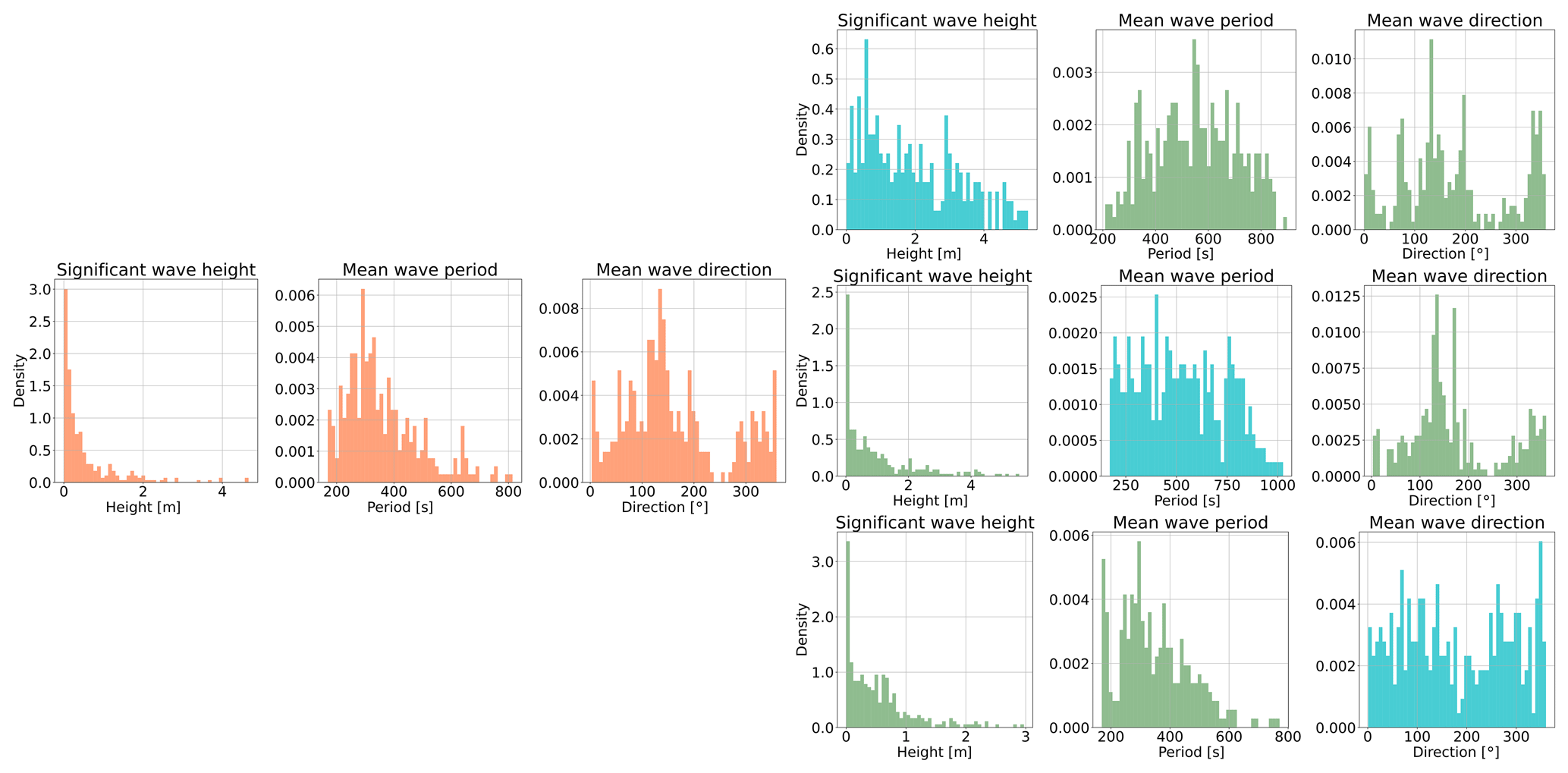
Figure 8 Random importance sampling's effect on the batch constitution during training. The single row on the left, with orange columns, represents the distributions of all three target variables in a random training batch without importance sampling. The three rows on the right display importance-sampled batches, each row belonging to a specific variable that was importance-sampled. The histograms coloured in blue contain those variables that were importance-sampled. Importance sampling results in more uniform distributions for the sampled variables, which indicates a more equal sampling of the target variable realisation space.

Neural networks often have difficulties predicting extreme events in the tails of the distributions because these events are by definition rare and the network rarely encounters them in the training set. To learn and model underrepresented values of the target variables better, we increased their presence in the training set by employing the so-called random importance sampling. We illustrate random importance sampling in Fig. 8. If we observe the distributions of the three target variables in a randomly sampled batch (left panel in Fig. 8), we can see that these are skewed. For example, the significant wave height is distributed similarly to a left-slanted gamma-like distribution with a very long tail. Therefore, the model is not exposed to the tail of the distribution frequently which inhibits efficient training in that part of the distribution. This results in systematic errors, where the regression accuracy for significant wave height drops with increasing height. This is understandable as samples with wave heights over 2 m constitute only a small fraction of the dataset, contributing less during training compared to samples with smaller wave heights.

Our implementation of importance sampling is conducted on the fly at batch acquisition. The reasons we do this on the fly as opposed to conducting this statically (oversampling before training and saving the new samples on disc) is the following: oversampling highly skewed distributions to a point of close uniformity would require a large number of additional samples. Since we had limited disc space, this was not an option. Therefore, we implemented single-variable importance sampling that oversamples one of the target variables at random for a given training batch. However, when we oversample one of the variables, the remaining usually remain biased. We can observe this effect in the skewed green histograms in Fig. 8, while the blue histograms are more uniform. To alleviate this issue, we alternated the sampling between the three target variables randomly to eliminate single-variable importance-sampling bias.

Furthermore, we alternated between regular sampling and importance sampling, where every second batch was randomly importance-sampled. This compromise offered the best performance out of the two approaches. We believe that this is due to the majority of data taking on only a small subset of values; thus, these values influence the loss more than the rare events. This is especially true for significant wave heights, where only 5 % of all samples across all locations exhibit wave heights over 2 m. Additionally, since fitting unbiased estimates of the tail of the distribution for significant wave heights was still challenging, we also penalised the network for misclassifying significant wave height twice as much as for the remaining two variables.

We conducted our training procedure in two stages. Since we trained our model on the Vega cluster (Institute of Information Science, 2023), we were limited by the maximum time our training could take up. A single run could last up to 2 d maximum; therefore, we first trained our model using the Adam solver (Kingma and Ba, 2014), with default PyTorch parameters, a learning rate of 10⁻³, and a weight decay of 10⁻⁶ for 2 d. Following this period, we extracted the model that performed on the validation dataset best, reinitialized the learning procedure with a reduced learning rate of 10⁻⁵, and retrained for 600 more epochs. We again took the model that performed on the validation dataset best and used it to compute the test dataset results we present in the following sections.

4 Temporal ablation study of the input

In this section, we investigate the impact of the number of time steps on the performance of the model. Adding multiple time steps results in inputting more information into the model; therefore, training performance might increase. However, due to overfitting, this performance might not be reflected in the actual accuracy using unseen data. Therefore, we conducted a preliminary comparison between five DELWAVE variants, each trained with a different number of input time steps. These variants are DELWAVE₂, DELWAVE₄, DELWAVE₈, DELWAVE₁₁, and DELWAVE₁₆, where the subscript denotes the number of time steps used. Here, each of the five variants uses n+1 time steps, where n denotes the number of previous time steps (in the case of DELWAVE₈, this means seven previous time steps, with the addition of the current one). The results of this study are presented in Table 1 and their validation loss during training in Fig. 9.

Table 1 Table containing the performance evaluations of DELWAVE, which we constructed by varying the number of time steps used during training, for three training locations: AA, MB, and OB. RMS denotes the root mean squared error, and the best-performing (with the lowest RMS) variant is in bold.

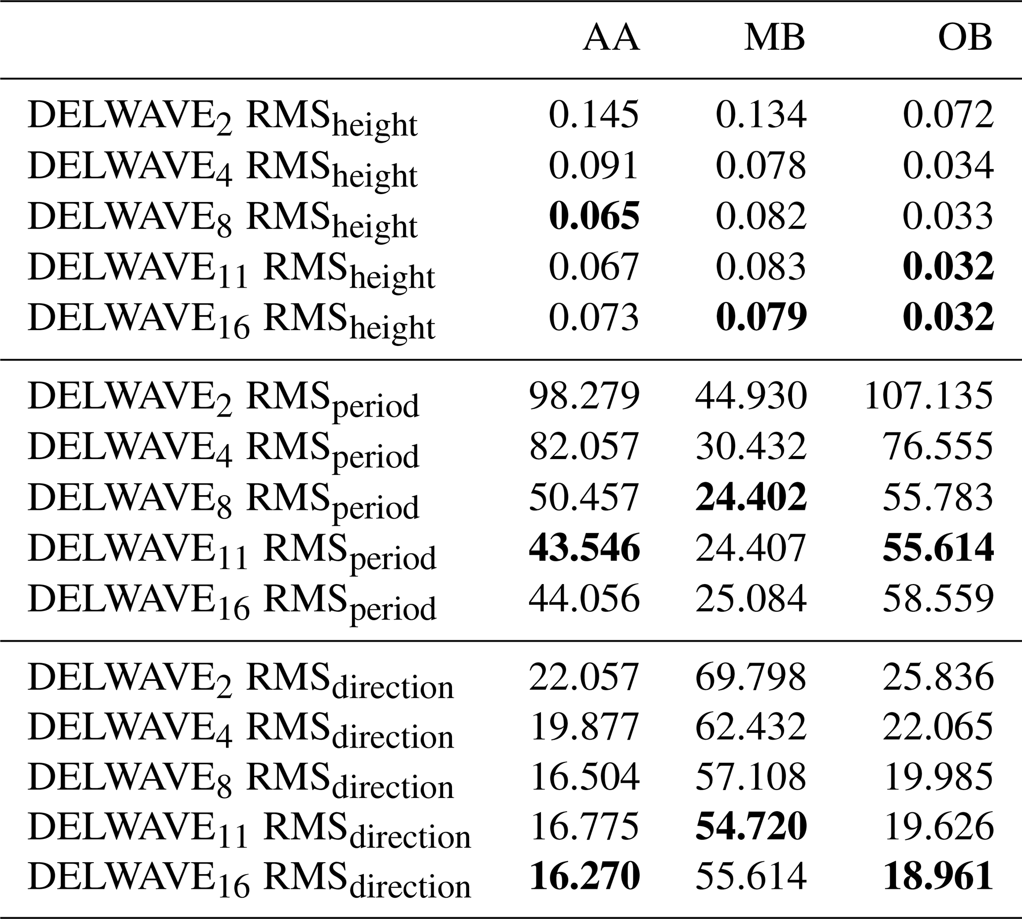
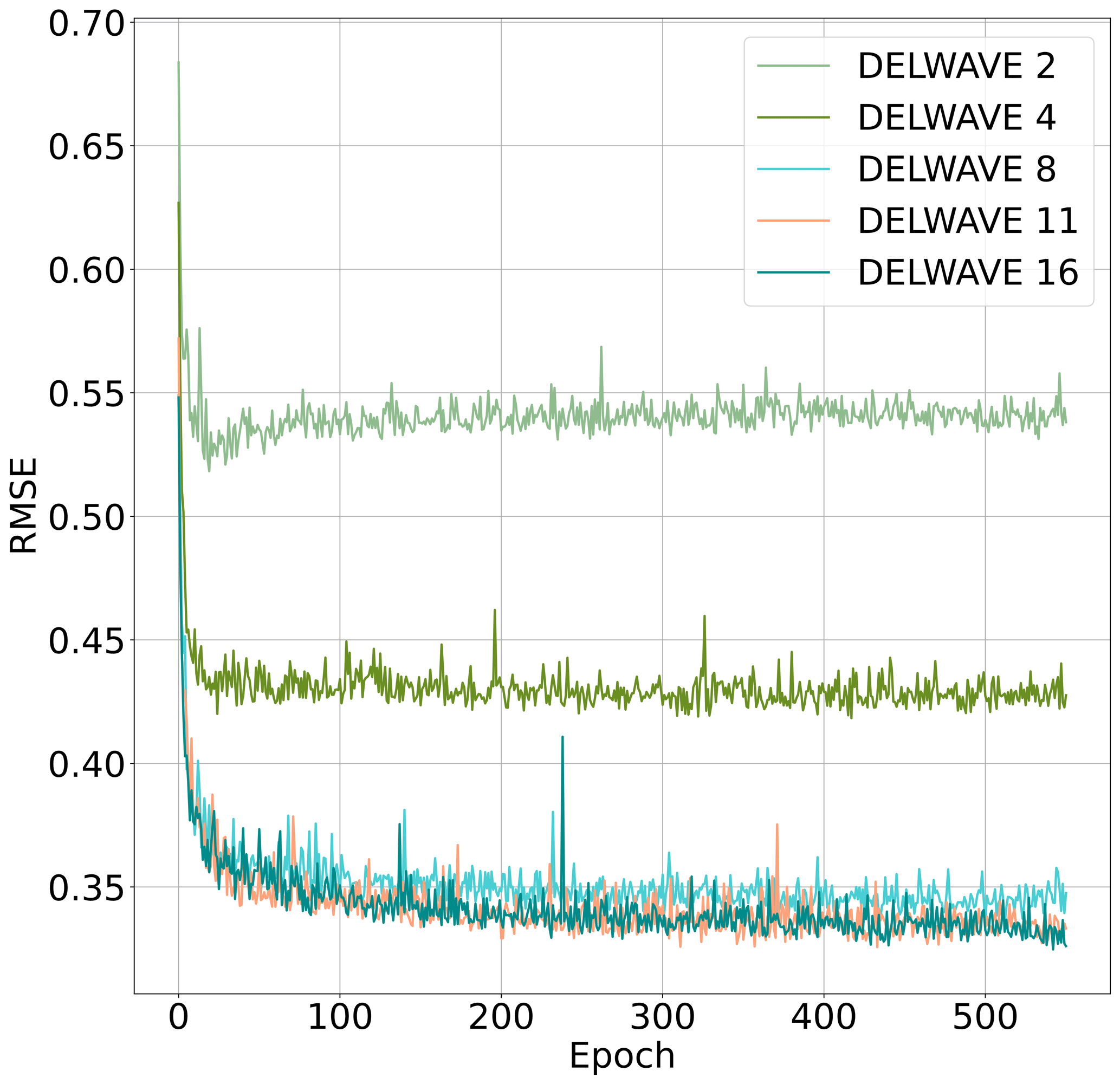
Figure 9 Root mean squared error in the validation dataset (averaged over all three variables) for all DELWAVE temporal ablation variants. The cutoff number of epochs is the amount achieved by DELWAVE₁₆ in 2 d of training since it is the slowest of all the variants.

We can observe the diminishing returns nature of adding time steps beyond the 11th time step; the performance seems to be roughly identical between DELWAVE₁₆ and DELWAVE₁₁. Also note that DELWAVE₁₆ contains more trainable parameters and is also slower to train compared to DELWAVE₁₁. DELWAVE₁₁ exhibits the best performance in four cases, which is equal to DELWAVE₁₆, followed by DELWAVE₈, with two cases. Similarly, we can observe that after the threshold of 11 time samples is reached, we enter the diminishing returns domain, where DELWAVE₁₆ offers negligible or even worse performance in some cases compared to DELWAVE₁₁. Therefore, we concluded that DELWAVE₁₁ is the most promising network variant for further training.

5 Results

In order to assess the potential and the possible limitations of the DELWAVE network, the analysis of the results is divided into three phases. After an overview of the performance of the network in reproducing the main overall properties of the SWAN time series (Sect. 5.1), the analysis focuses on two aspects of particular relevance for practical purposes – namely, the capability of reproducing storms (including, but not limited to, extreme events; Sect. 5.2) and their main properties and the capability of capturing the main features of the climate change signal (Sect. 5.3).

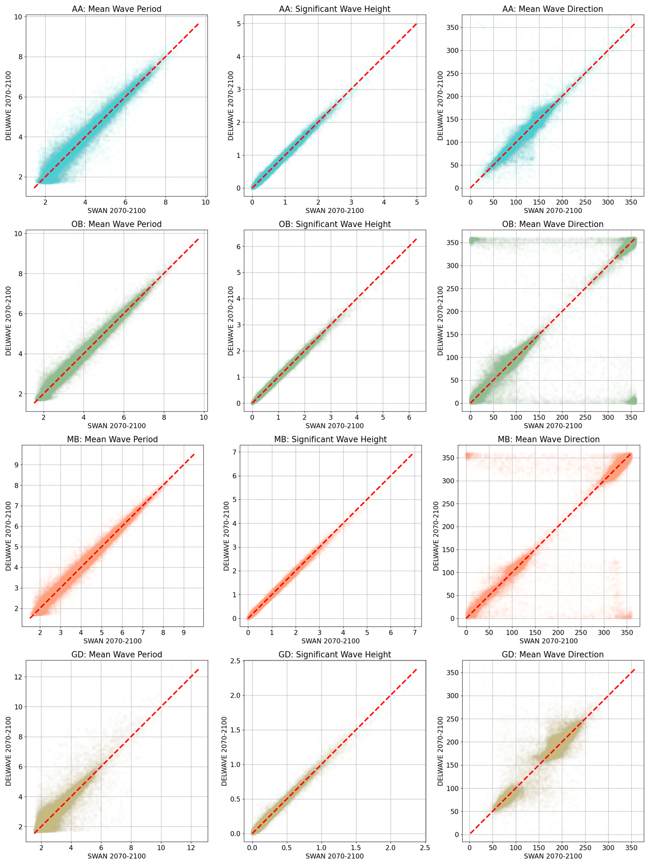
Figure 10 A scatterplot of DELWAVE forecasts (y axis) compared to their SWAN targets (x axis) the for mean wave period [s] (first column), significant wave height [m] (second column), and mean wave direction [°] (third column) at AA (first row), OB (second row), MB (third row), and GD (fourth row). Mean wave directions are listed in nautical notation (0° representing north, 90° representing east, etc.). The dashed diagonal line in each plot indicates a perfect forecast.

5.1 Deep network vs. SWAN in the far-future climate of 2071–2100

In this section, we present DELWAVE performance during the far-future period of 2071–2100, as benchmarked against SWAN simulations. In other words, SWAN simulations represent the ground truth DELWAVE aims to model. Figure 10 depicts DELWAVE–SWAN scatterplots of H_s, d, and $T_{\mathrm{m}-\mathrm{1},\mathrm{0}}$ at the locations of the Acqua Alta oceanographic tower (AA) and the Ortona and Monopoli buoys (OB and MB, respectively; see Fig. 2 for the locations). Results for other locations are provided in the Supplement.

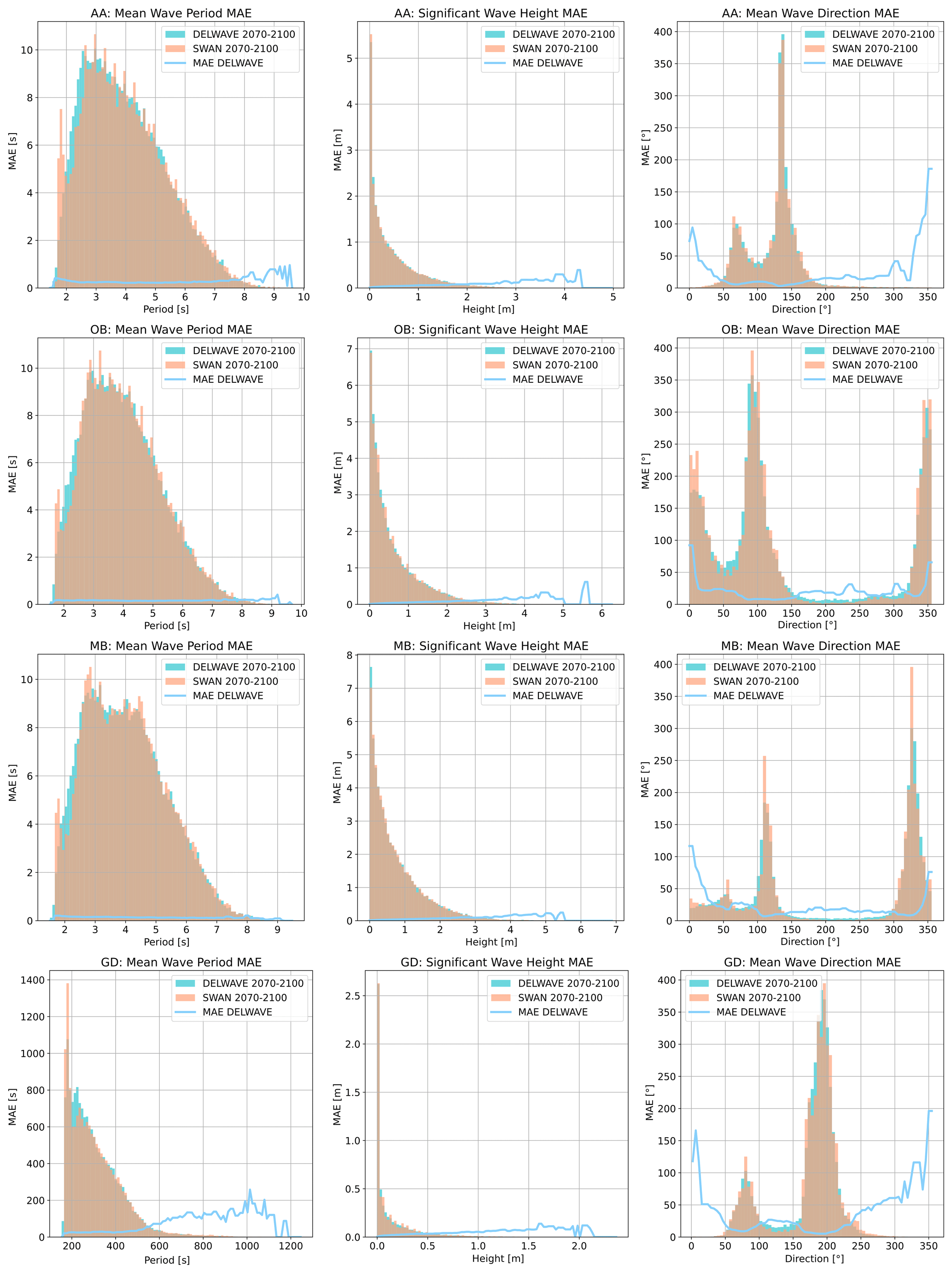
Figure 11 Histograms of DELWAVE vs. SWAN distributions of H_s (left column), d (middle column), and $T_{\mathrm{m}-\mathrm{1},\mathrm{0}}$ (right column) from the DELWAVE (turquoise bars) and SWAN models (brown bars) during the 2071–2100 time window at AA (first row), OB (second row), MB (third row), and GD (fourth row). Light blue lines are scaled on the y axis and depict MAE averaged over a number of samples in each bin.

We proceed by analysing DELWAVE performance using three related figures. Figure 10 depicts DELWAVE predictions for H_s, d, and $T_{\mathrm{m}-\mathrm{1},\mathrm{0}}$ compared to those from the SWAN model, obtained from the same wind fields, i.e. for the same forecasting time window. Figure 11 shows the overlaps of histograms of H_s, d, and $T_{\mathrm{m}-\mathrm{1},\mathrm{0}}$ from both DELWAVE and SWAN models. Note that close overlap of the distribution histograms from both models does not guarantee a good forecast since this overlap does not say anything about the synchronicity of both forecasts; one therefore needs to view Fig. 11 in conjunction with Fig. 10. Additionally, Fig. 11 illustrates how DELWAVE forecasting mean absolute errors change depending on which part of distribution we are modelling. Here, mean errors imply error averaging over all the forecasting samples in a specific distribution bin. Consequently, the error values are only well defined in the bins containing a large enough (e.g. over 100) number of samples. In what follows, we base our remarks on an interplay of messages from all three figures.

Location AA in the northern Adriatic (off the Venetian shore; see Fig. 2 for the location) is marked by an excellent performance in H_s and d prediction, indicated by the near-linear scatterplot displayed in Fig. 10. The same aspect of DELWAVE performance is illustrated via histogram distribution for the same three parameters in Fig. 11. Mean wave direction d (top row, right column of Fig. 11) exhibits two maximums related to two dominant Adriatic winds, northeasterly Bora at roughly 75° and southeasterly Scirocco at roughly 135°. Short wave periods at the AA location, on the other hand, seem to be the hardest to predict, as can be seen from in the left column in either Fig. 10 or Fig. 11. This is, to some extent, expected: long wave periods correspond to longer waves and consequently windy atmospheric conditions. Short periods, on the other hand, correspond to calm conditions, where the network is essentially modelling low-amplitude, short-wavelength, stochastic sea surface behaviour.

Similar observations can be made for OB and MB locations. SWAN H_s is modelled very reliably with DELWAVE. Multi-modal direction histograms at all locations are also reproduced to a high degree of accuracy, as can be seen from the middle column of Fig. 11. On the other hand, the network seems to be struggling to reproduce northerly directions (roughly 0° ± 10°) at this location. This leads to horizontal strips of incorrect predictions displayed in the scatterplot of the right column, second row in Fig. 10 and to a bump in mean absolute error in the histogram displayed at the same location in Fig. 11.

Figure 11 also hints at quantitative estimates of DELWAVE performance. When it comes to H_s predictions (middle column), errors at all locations grow with significant wave height from errors below 5 cm for H_s below 1 m to errors on the order of 10–15 cm for H_s over 3 m. DELWAVE predictions of mean wave direction d (right column) exhibit the smallest errors in the directional bins corresponding to prevalent wind patterns. In general, directional errors are below 25° and even lower at AA. High directional errors at 0 and 360° stem at least partly from the algorithm's false distinction between 0 and 360° directions.

Wave period $T_{\mathrm{m}-\mathrm{1},\mathrm{0}}$ predictions are illustrated in the left column of Fig. 11. At all locations, periods below 6 s are captured well by DELWAVE, with prediction errors below 0.25 s. Longer periods, however, likely corresponding to an incoming swell, exhibit more diverse behaviour. MB location wave periods seem to be captured more accurately in the long-period limit, with the forecast error dropping below 0.1 s. At the OB location, the errors in the long-period limit slightly rise from 0.2 to 0.3–0.5 s. The AA location, on the other hand, indicates a sharp rise in the $T_{\mathrm{m}-\mathrm{1},\mathrm{0}}$ prediction error, which reaches 1 s for the period above 8 s.

The error behaviour at the AA location is possibly explained by the differing roles played by the basin geometry, the local wind sea, and swell. Location AA is prevalently exposed to northeasterly Bora (blowing from roughly 75°) and to southeasterly Scirocco (blowing from 135°). In the case of Bora, the fetch is quite limited since Bora is a cross-basin wind. Therefore, we do not expect swell to play a major role at the AA location during Bora conditions: the wave field at the AA location must be determined by local wind conditions. The case of Scirocco is very different. Scirocco is an along-axis wind, with the largest fetch in the Adriatic Basin. This means that during Scirocco, the swell field at AA is determined to a large extent by non-local wind patterns in the south of the basin. Local wind conditions at the AA location are furthermore often a poor proxy for winds in the south Adriatic. Bora in the north (promoting short fetch and shorter wave periods) coinciding with Scirocco in the south (promoting long-period swell arriving at AA) is, for example, not unusual. These circumstances likely pose a challenge for the DELWAVE deep network, resulting in growing errors during longer wave periods (which most likely occur during Scirocco).

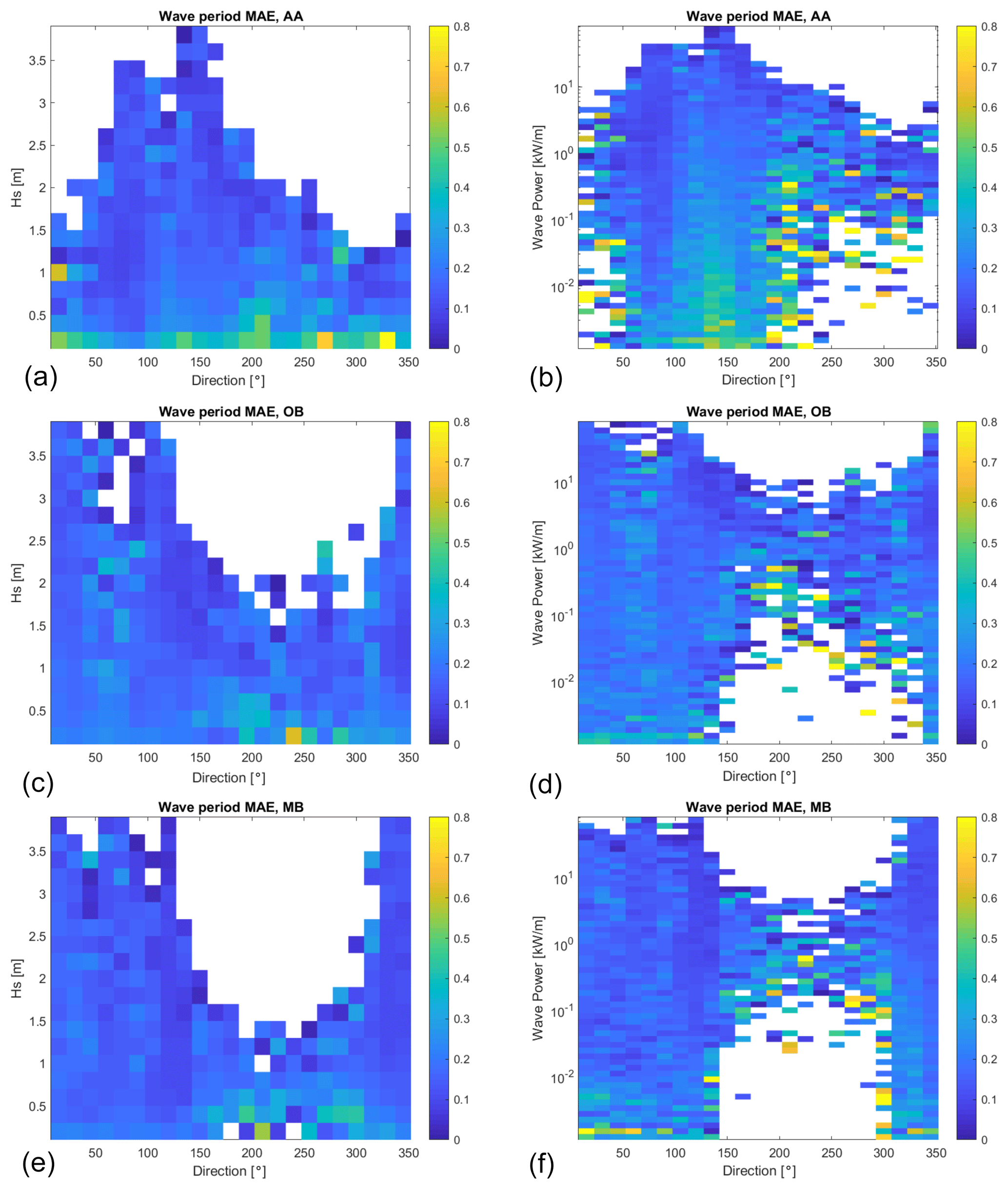
Figure 12 Comparison of the wave period (indicated by colour) relationship to significant wave height, H_s (a, c, and e; y axis), and to wave power (b, d, and f; y axis) in all directions (x axis) for AA (a, b), OB (c, d), and MB (e, f). The white parts in the plot refer to combinations of the direction and variable for which no occurrence was found in the data.

This explanation can be further substantiated by comparing wave period MAE to H_s, $T_{\mathrm{m}-\mathrm{1},\mathrm{0}}$, and wave power. The latter is computed from the linear theory to be

$$\begin{array}{}\text{(13)}& P={\displaystyle \frac{\mathit{\rho }{g}^{\mathrm{2}}}{\mathrm{64}\mathit{\pi }}}{H}_{\mathrm{s}}^{\mathrm{2}}{T}_{\mathrm{m}-\mathrm{1},\mathrm{0}},\end{array}$$

with ρ being the water density and g the acceleration due to gravity. This comparison is depicted in Fig. 12, which corroborates this interpretation and constrains DELWAVE limitations in capturing the basin-scale dynamics.

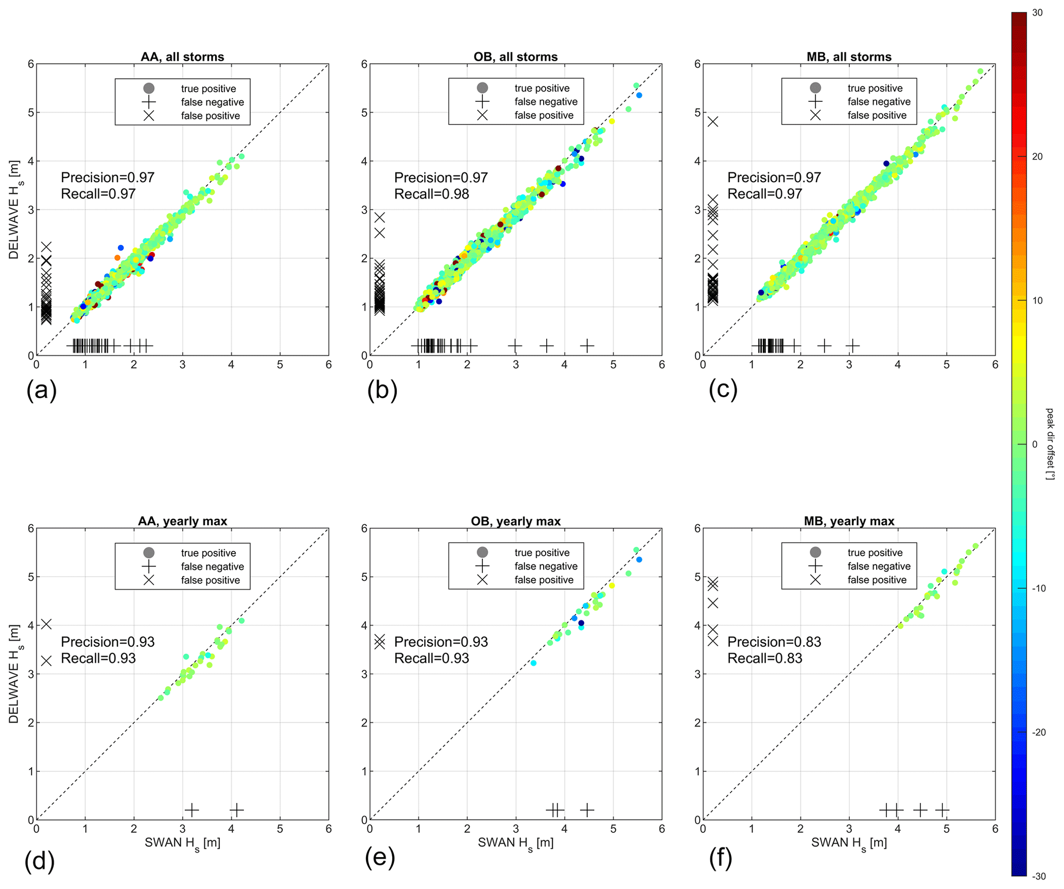
Figure 13 Comparison of SWAN and DELWAVE peak H_s values at AA, OB, and MB during all the storms (a, b, c) and for the annual maxima (d, e, f). The dashed diagonal line indicates a perfect match. The colour map represents the directional offset during the peak of each storm. Pluses and crosses along the plot axes represent false negatives (+) and false positives (×).

Figure 14 Examples of false negatives (a) and false positives (b) in the identification of storms (thick lines), following the method by Boccotti (2000) in the DELWAVE and SWAN H_s time series (thin lines). The dotted lines represent the reference threshold of $\mathrm{1.5}\stackrel{\mathrm{‾}}{H_{\mathrm{s}}}$ for each time series.

The concentration of the highest values of MAE at low values of H_s and P (left and right columns, respectively) confirms that largest errors tend to be associated with low-energy, nearly random sea states, even in the presence of relatively long waves along the main basin axis (Scirocco at AA), and thus with limited impacts on possible practical applications. It is further worth mentioning that a separate analysis, carried out by independently considering the rising and declining phases of the sea states (not shown), did not exhibit any preferential concentration of the higher values of MAE in either phase. Wave period error is therefore not systematically larger during either onset or calming of the storm, suggesting that it is not directly related to the sequential and monotonous temporal encoding of inputs within DELWAVE. Had this not been the case, we would have expected some error asymmetry with regard to the timing of the storm.

5.2 Storm analysis

The analysis of the storms was carried out by comparing the DELWAVE results to the SWAN time series during the period of 2071–2100. For each time series, the storms were identified following the method proposed by Boccotti (Boccotti, 2000) – namely, (i) finding the events with H_s larger than 1.5 times the mean value $\stackrel{\mathrm{‾}}{H_{\mathrm{s}}}$ of each respective series, (ii) merging the events parted by less than 10 h, and (iii) discarding those overall shorter than 12 h. Figure 13 compares SWAN and DELWAVE peak H_s and directions for each storm at AA, OB, and MB (the same is shown for the other locations in the Supplement), considering entire sets of storms occurring during the period separately and the annual maxima for each series. While the former provides a broader view on how DELWAVE reproduces the whole meteo-marine climate at each location, the latter aims at assessing its capability of addressing extreme events. The picture is flanked by a quantification of the DELWAVE precision (how many DELWAVE-predicted storms are actually present in the SWAN time series) and recall (how many SWAN-modelled storms are retrieved by DELWAVE). These two metrics are computed as

$$\begin{array}{}\text{(14)}& \text{precision}={\displaystyle \frac{\text{TP}}{\text{TP}+\text{FP}}},\text{recall}={\displaystyle \frac{\text{TP}}{\text{TP}+\text{FN}}},\end{array}$$

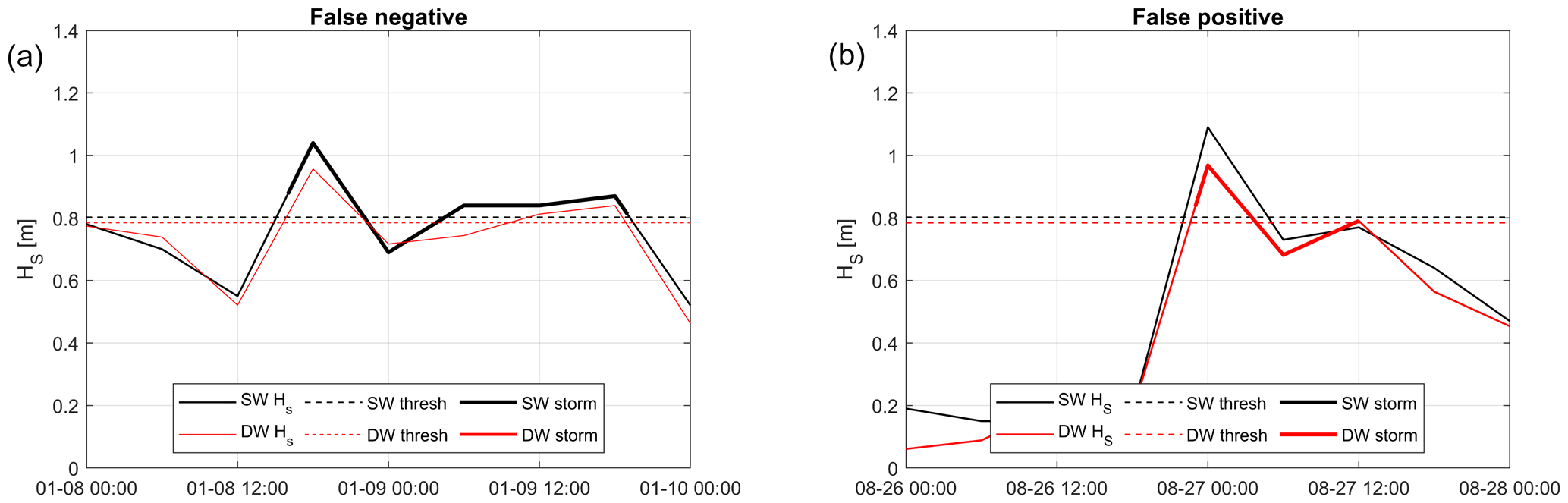
where TP, FP, and FN denote true positive (storm present in SWAN and predicted by DELWAVE), false positive (storm predicted by DELWAVE but not present in SWAN), and false negative (storm present in SWAN but not predicted by DELWAVE) classifications. Figure 14 shows an example of the application of Boccotti's method in SWAN and DELWAVE storms and the occurrence of false negatives and false positives.

All considered sets exhibit a satisfactory performance with very high scores (precision and recall ≥ 0.95) when all the storms are considered. When only annual maxima are taken into account, precision and recall are lower, though fairly high (≥ 0.8) and without an evidently prevailing directional offset. Considering the whole storm sets, most of the false negatives and positives are generally clustered among the weakest events. This can be explained by considering that, for particularly weak or short events, small absolute errors can mean large relative errors. Therefore, in a small H_s limit, a small error in the reproduction of H_s can already significantly impact whether the criteria for the identification of storms are met or not (Fig. 14).

This result seems to be in contradiction with the results for the yearly maxima sets, where prediction and recall scores decrease and the number of false negatives and positives increases. This contradiction is, however, only apparent and related to the propagation of H_s prediction errors downstream into the identification of the yearly maxima. More precisely, in this case, the mismatch does not seem related to the classification of an event as a storm but rather to its classification as a yearly maximum: in fact, a slight error in predicting the peak height of storm events can introduce some noise in the ranking of the events and, in particular, in the identification of the yearly maxima, leading to a mismatch between DELWAVE and SWAN. Nonetheless, as long as small errors in the prediction of the peak H_s are the cause for this mismatch, even if the events retrieved by DELWAVE are not exactly the ones resulting from the SWAN time series, their properties (or at least their peak H_s) should be quite close, which should be sufficient for most practical applications.

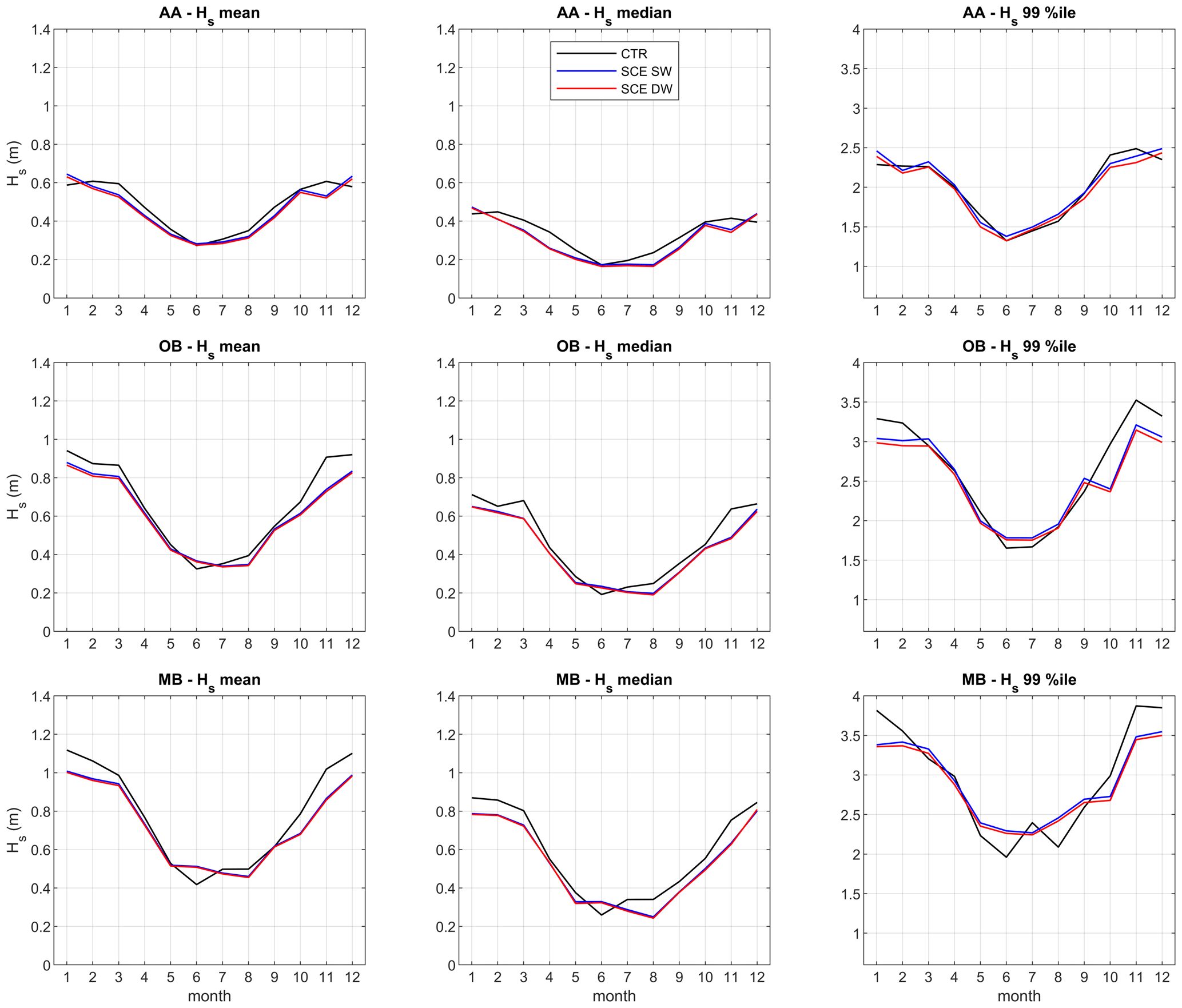
Figure 15 Comparison of SWAN (SW) and DELWAVE (DW) mean, median, and 99th-percentile H_s climatology statistics in the future scenario (2071–2100; SCE), with the SWAN-modelled statistics referring to the control period (1971–2000; CTR) at AA, OB, and MB, respectively.

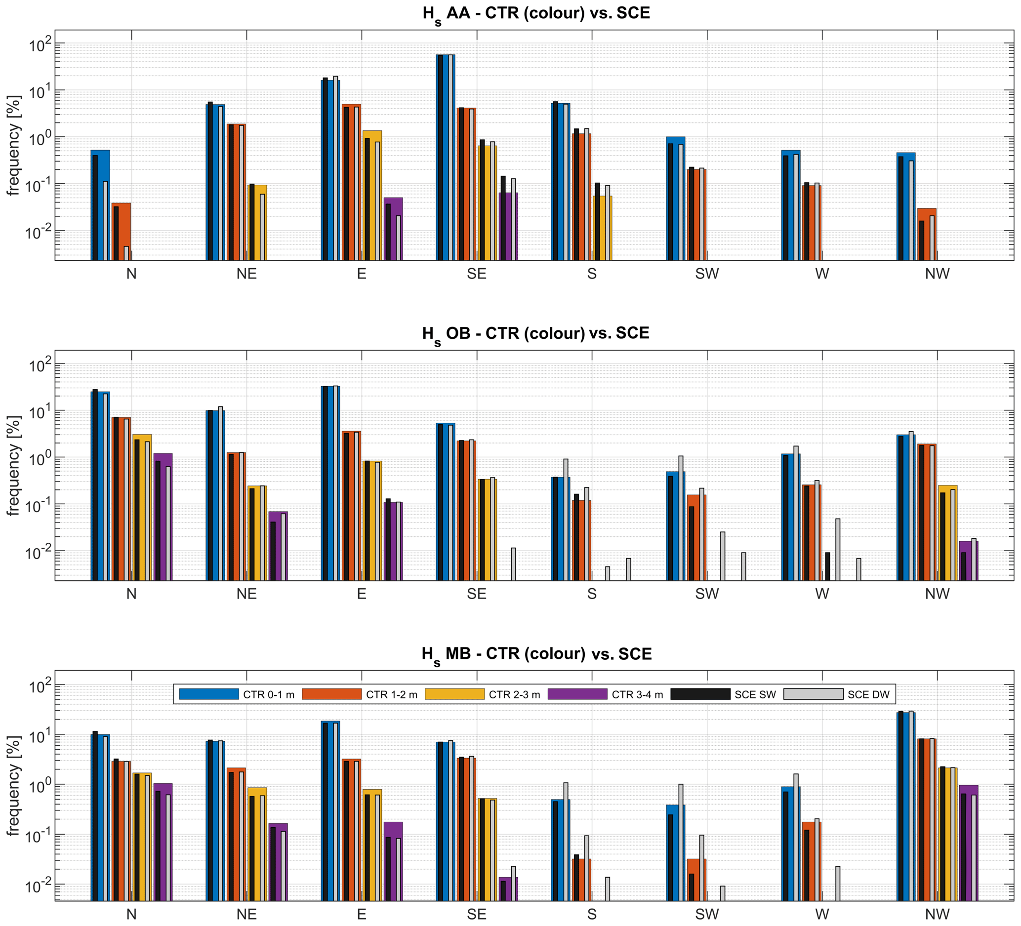
Figure 16 Comparison of SWAN (SW) and DELWAVE (DW) directional H_s statistics in the future scenario (2071–2100; SCE; black and grey bars, respectively), with the same quantities modelled by SWAN, in reference to the control period (1971–2000; CTR; coloured bars) at AA, OB, and MB, respectively.

5.3 Climate change features

One of the main scopes of DELWAVE is to provide a computationally cheap model emulation system capable of providing large ensemble predictions for wave climate at a multi-decadal scale. This kind of applications is, to some extent, complementary to the event-scale analysis of single storms and requires a specific assessment of the network capability of capturing the main statistical features of the climate signal. Figure 15 provides a twofold comparison of the climatological normals of the monthly mean, median, and 99th percentile of H_s at AA, OB, and MB (the same values for the other locations are provided as a Supplement) provided by SWAN and reproduced by DELWAVE. The statistics resulting from SWAN and from the DELWAVE time series are compared to each other in the end-of-century scenario (2071–2100; SCE), and both are compared to the statistics from the control condition (CTR), available only for SWAN in the 1971–2000 period. The good agreement between DELWAVE and SWAN is also confirmed when considering climatological statistics, with a small (≤ 5 %), though systematic, underestimate of 99th-percentile values, reflecting what was discussed in Sect. 5.1. Compared to the CTR climatologies, the mismatch between DELWAVE and SWAN is generally small compared to the difference between SCE and CTR conditions, suggesting that the noise possibly introduced by the model mimicking is weaker than the climate change signal in the considered locations. Not surprisingly, the only way in which the performance seems partially affected by seasonality is through the modulation of significant wave height and the tendency of the network to underestimate higher (and therefore wintry) values. Nevertheless, Fig. 15 shows that the potential modelling errors, introduced by the DELWAVE model, are substantially smaller than the difference between the scenario (2070–2100) and control periods (1970–2100).

Following a similar approach for the directional wave climate, the linearised wave roses in Fig. 16 show that the agreement between DELWAVE and SWAN allows us to capture important impacts of climate change in the wave regime not only in absolute terms, but also in response to projected shifts in the wind regimes. This is, for instance, the case of the slight weakening of Bora (NE) storms associated with an intensification of Scirocco (SE) events in the northern Adriatic Sea in the broader framework of a tendency towards an overall decrease in the storminess in most of the basin, suggested by Bonaldo et al. (2020) and confirmed by the DELWAVE projections.

6 Conclusions

We present a new point-prediction deep learning method for surface gravity wave emulation in epicontinental Adriatic Basin, which took about 2.5 d to train and can process more than 100 wind fields per second, to be used for large-ensemble prediction over synoptic to climate timescales. The DELWAVE input set consists of atmospheric winds during 1998–2000, and the test period is the far-future climate time window of 2071–2100. We have thoroughly analysed which architecture yields the best results for wave emulation and these efforts led us to the presented architecture of a convolution-based atmospheric encoder block, a temporal collapse block, and finally a regression block. We introduced random importance sampling for improved modelling of underpopulated tails of variable data distributions. Detailed ablation studies were performed to determine optimal performance regarding the input fields, temporal horizon of the training set, and network architecture. We demonstrated that DELWAVE reproduces SWAN model significant wave heights with a mean absolute error (MAE) between 5 and 10 cm, mean wave directions with a MAE of 10–25°, and mean wave period with a MAE of 0.2 s. The network is able to accurately emulate multi-modal distributions of mean wave directions, which are related to dominant wind regimes in the basin. An analysis of DELWAVE performance during storms was performed by employing threshold-based metrics of precision and recall. DELWAVE reached a very high score (both metrics over 95 %) of storm detection.

SWAN and DELWAVE time series are further compared to each other in the end-of-century scenario (2071–2100), and both are compared to control period of 1971–2000. Compared to control climatology over all wind directions, the mismatch between DELWAVE and SWAN is generally small compared to the difference between scenario and control conditions, suggesting that the noise introduced by surrogate modelling is substantially weaker than the climate change signal. There is a number of things we would like to explore further: it is currently not clear how to leverage Gaussian (or other) spatial encoding to generate, if possible, reliable predictions for locations which lie outside of the training set. This might open the door for dense predictions of the wave field, at least in the vicinities of input data locations. It would furthermore be interesting to introduce temporal dependence of the Gaussian variances in the spatial encoding matrix to help the network focus on wider areas of input data as we feed it data from a more distant past.

Future research and potential applications may also focus on the larger scales – for example, the entire Mediterranean Sea basin – using a high-resolution wind and waves model to boost DELWAVE training. The objective would be to explore the behaviour of numerical and machine learning models in diverse wind and wave regimes, as well as wind and marine storms, which exhibit distinct physical characteristics in a basin with highly diverse morphological and dynamic features.

Last but not least, another promising venue is offered by recent developments in the field of physics-informed machine learning. Here, the solution subspace is further constrained by additional loss terms, which nudge the learning process towards physically consistent solutions. Since the physical aspects of wind-driven surface gravity waves are known in substantial detail, we expect there to be some immediate benefits to introducing dynamics laws into the training. Last but not least, it would be interesting to study how well the network generalises to other domains and other models. All these will be topics of further research.