A general comprehensive evaluation method for cross-scale precipitation forecasts

With the development of refined numerical forecasts, problems such as score distortion due to the division of precipitation thresholds in both traditional and improved scoring methods for precipitation forecasts and the increasing subjective risk arising from the scale setting of the neighborhood spatial verification method have become increasingly prominent. To address these issues, a general comprehensive evaluation method (GCEM) is developed for cross-scale precipitation forecasts by directly analyzing the proximity of precipitation forecasts and observations in this study. In addition to the core indicator of the precipitation accuracy score (PAS), the GCEM system also includes score indices for insufficient precipitation forecasts, excessive precipitation forecasts, precipitation forecast biases, and clear/rainy forecasts. The PAS does not distinguish the magnitude of precipitation and does not delimit the area of influence; it constitutes a fair scoring formula with objective performance and can be suitable for evaluating rainfall events such as general and extreme precipitation. The PAS can be used to calculate the accuracy of numerical models or quantitative precipitation forecasts, enabling the quantitative evaluation of the comprehensive capability of various refined precipitation forecasting products. Based on the GCEM, comparative experiments between the PAS and threat score (TS) are conducted for two typical precipitation weather processes. The results show that relative to the TS, the PAS better aligns with subjective expectations, indicating that the PAS is more reasonable than the TS. In the case of an extreme-precipitation event in Henan, China, two high-resolution models were evaluated using the PAS, TS, and fraction skill score (FSS), verifying the evaluation ability of PAS scoring for predicting extreme-precipitation events. In addition, other indices of the GCEM are utilized to analyze the range and extent of both insufficient and excessive forecasts of precipitation, as well as the precipitation forecasting ability for different weather processes. These indices not only provide overall scores similar to those of the TS for individual cases but also support two-dimensional score distribution plots which can comprehensively reflect the performance and characteristics of precipitation forecasts. Both theoretical and practical applications demonstrate that the GCEM exhibits distinct advantages and potential promotion and application value compared to the various mainstream precipitation forecast verification methods.

1 Introduction

Precipitation is one of the most important forecasting elements in weather forecasting (Bi et al., 2016; Han et al., 2023). Short-duration heavy rainfall often leads to flooding and geological disasters, causing widespread and severe impacts (Zhong et al., 2022; Yang et al., 2023). Precipitation forecasts, as focuses and challenges in meteorological department operations, have drawn widespread attention from governments, societies, and the public (Bi et al., 2016; Hao et al., 2023). Scientifically evaluating precipitation forecasts helps people gain a clear understanding of the current precipitation forecast levels and maintain appropriate psychological expectations for such forecasts. Moreover, such evaluations assist forecasters in rationally analyzing the quality and characteristics of quantitative precipitation forecast systems and aid researchers in understanding the level, strengths, and weaknesses of various types of forecasting systems, which, in turn, offers valuable insights to improve these systems (Zhong et al., 2022; Zhang et al., 2022; J. Liu et al., 2022; Gofa et al., 2018). However, there are several shortcomings in the current precipitation verification approaches. For instance, with traditional scoring methods, small errors in the location or timing of convective features can lead to false alarms and missed events, and their utility is limited regarding diagnosing model errors such as a displaced forecast feature or an incorrect mode of convective organization; thus, traditional scoring methods often fail to reflect model performance improvements (Ahijevych et al., 2009). For high-resolution precipitation forecasts, even if the spatial distribution and intensity of precipitation are consistent with the observations, slight spatial and temporal deviations between forecasts and observations may still result in a large false alarm ratio and missed alarm ratio, leading to lower forecast scores (Zhao and Zhang, 2018). With the rapid development of seamless fine quantitative precipitation forecasts, the need for objective and rational evaluations of the accuracy and characteristics of precipitation forecasts has become increasingly important and urgent (Chen et al., 2021).

Precipitation forecast verification involves various methods, including traditional contingency-table-based classification verification and spatial verification methods. The traditional verification method can be traced back to 1884 when Finley introduced a dichotomous contingency table for tornado forecasts and evaluated these forecasts using the proportion correct scoring method (Finley, 1884). Subsequently, systematic attention was given to the evaluation of forecast classification methods, and Finley's forecast verification method became a classic example of the discussion of forecast scoring methods (Murphy, 1996). Gilbert (1884) proposed two scoring methods, namely the ratio of verification and the ratio of success in forecasting. The ratio of verification later became known as the threat score (TS) (Palmer and Allen, 1949) or the critical success index (Donaldson et al., 1975; Mason, 1989). The ratio of success is referred to as the Gilbert skill score (GSS) (Schaefer, 1990) or the equitable threat score (ETS) (Doswell et al., 1990; Gandin and Murphy, 1992). The TS encourages correct event forecasts (hits) and accounts for the impacts on the false alarm and missed alarm ratios, which can better guide forecasters or research and development personnel in making reasonable subjective and objective predictions compared to relying solely on simple “accuracy”. Meanwhile, the ETS eliminates the influence of random forecasts on the score, resulting in a fairer skill score (C. Liu et al., 2022).

In addition to the TS and ETS, the methods of traditional contingency-table-based classification verification include the Peirce skill score (PSS) (Peirce, 1884; Hanssen and Kuipers, 1965; Murphy and Daan, 1985; Flueck, 1987), Heidke skill score (HSS) (Doolittle, 1885, 1888; Heidke, 1926), probability of detection (POD), frequency bias (BIAS), accuracy (ACC), false alarm ratio (FAR), missing ratio (MR), and probability of false detection (POFD). The PSS is a fair score index that is equal to the hit rate minus the false detection probability; the HSS eliminates the influence of random forecasts, and the results can reflect the forecast skill (C. Liu et al., 2022). Many studies have reviewed and compared these two scoring methods (Doswell et al., 1990; Schaefer, 1990; Marzban, 1998; Mason, 2003). In extreme-weather-event verification (including severe convective weather such as short-duration heavy rainfall), the traditional scoring methods (such as the TS and ETS) for dichotomous events often yield scores of zero when the occurrence probability of the object being verified is very low. Therefore, Stephenson et al. (2008) proposed the extreme-dependency score (EDS) for evaluating extreme events. The EDS has the advantage that different forecast systems converge to different values and has no explicit dependence on the bias of the prediction system (Stephenson et al., 2008; Casati et al., 2008).

It has been more than a century since Gilbert (1884) proposed two scoring concepts, i.e., the ratio of verification and the ratio of success in forecasting (later known as the TS and ETS). The TS and ETS have been widely used for the performance evaluation of threshold-based event forecasts despite their evident shortcomings (Stephenson et al., 2008). Today, in various forecast verification applications, including high-resolution quantitative precipitation and extreme weather forecast verification, the TS and ETS remain mainstream approaches (Tang et al., 2017; Wei et al., 2019; Chen et al., 2021; Liu et al., 2023). With the continuous introduction of new scoring methods, several problems in traditional verification have been solved. However, the advantageous position of the TS remains unchallenged. Although the reasons for this are varied, its objectivity and practicality merit attention.

The traditional TS categorizes precipitation according to thresholds and performs verification using a dichotomous contingency table. The TS can be viewed as a measure of forecast accuracy that excludes hit forecasts for “non-occurrence” precipitation events (referred to as no precipitation), and its calculation formula is simple, objective, and standardized. However, there are two main limitations of the TS. First, precipitation is categorized by thresholds based on the contingency table, which has limitations in terms of classification. The drawback of artificially dividing precipitation into different threshold ranges is that it cannot guarantee that two adjacent precipitation values will always fall within the same threshold range. Slightly different precipitation values are not within the same threshold, which can lead to precipitation score distortion. The second limitation is related to the so-called “double-penalty” issue. With the development of high-resolution numerical weather forecasting and the shortening of the spacing between model grid points, some meso- and small-scale phenomena have been portrayed by models. However, it is difficult for high-resolution numerical forecasts to match the characteristics of the observed meso- and small-scale forecasts, resulting in traditional scoring methods often being unable to reflect these improvements in terms of model performance. Assuming a constant forecast area when there is a small deviation in the timing and location of events between a forecast and an observation, both “false alarms” and “missed alarms” will occur, which is referred to as the double-penalty phenomenon. This phenomenon leads to a score lower than the subjectively expected result, making it difficult to obtain appropriate verification scores when a forecast that “looks good” is not as good as one that “looks bad” (Ahijevych et al., 2009; Wilks, 2006; Ebert, 2008; Chen et al., 2021). For low-probability events with limited sample size for verification, such as torrential rain and short-term heavy rainfall, the double-penalty issue becomes more prominent. The TS and ETS for torrential rain are often at the unskilled end of the scoring values (Chen et al., 2019). In recent years, new mainstream scoring methods have addressed most of the abovementioned limitations but still have shortcomings. Such methods include the improved gradient decreasing method, which still results in poor scores for good forecasts, and the neighborhood spatial verification method, which has too many subjective components and may miss meso- and small-scale information.

Table 1 Gradient decrease scoring table for station-by-station (time) rainstorm forecasts. The values are normalized, i.e., score = original data $/$ 100.

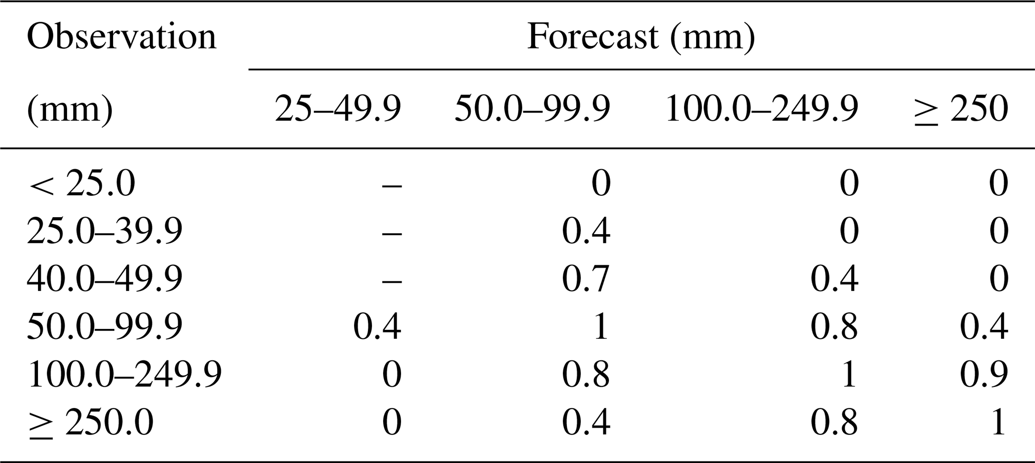
Table 2 Examples of station-specific rainstorm precipitation scoring.

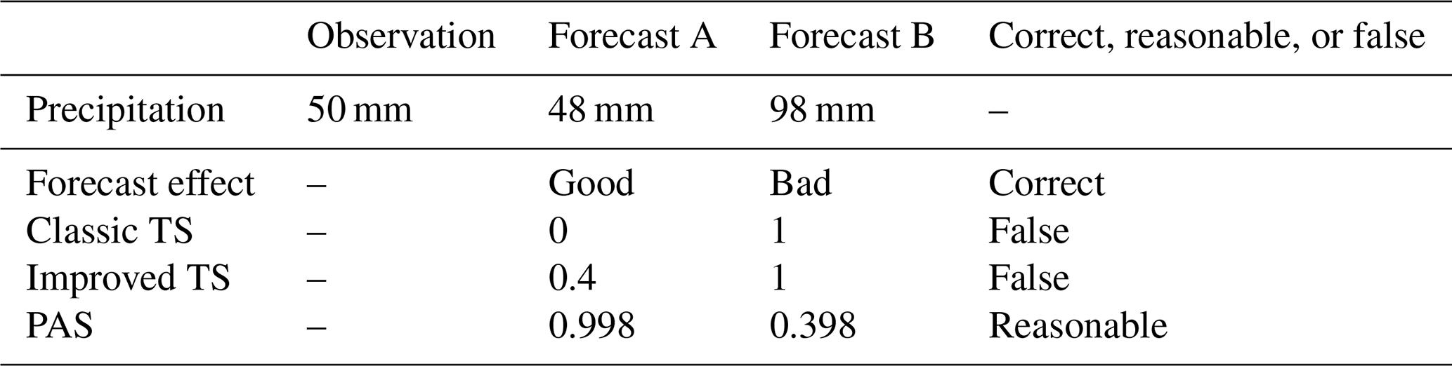
To address the limitations of threshold-based precipitation classification and improve the verification effect, e.g., the gradient decreasing method (hereinafter referred to as the magnitude-improved TS) is used to verify the accuracy of rainstorm forecasts (Yang et al., 2017), and appropriate weights are assigned to close forecast values to avoid scores of zero (Table 1). However, the magnitude-improved TS still has limitations. For example, if the observed 24 h accumulated precipitation is 50 mm when forecast A is 48 mm and forecast B is 98 mm, then forecast A is evidently better than forecast B. According to the original TS, forecast B scores 1 point, while forecast A does not score any points. For the magnitude-improved TS, forecast B scores 1 point as it still falls within the same magnitude category as the observed precipitation, while forecast A scores only 0.4 points; this still fails to reflect the fact that forecast A is superior to forecast B (Table 2). By employing the new scoring method, i.e., the precipitation accuracy score (PAS), which will be discussed later, forecast A scores 0.998 points, while forecast B scores 0.398 points, confirming the rationality and validity of this new method.

To address the double-penalty issue, a common approach is to employ the neighborhood spatial verification method (also known as the fuzzy method) which has two specific processing forms. The first approach is simple upscaling, which uses a certain method (such as value averaging, maximum, and value weighting) to select values within the scale range (Chen et al., 2019), adjusting the high-resolution forecast and observation information to a larger scale to reduce the accidental information of high-resolution data, and then using the traditional skill score (Yates et al., 2006; Weygandt et al., 2004). The other form is the improved neighborhood spatial verification method proposed by Roberts and Lean (2008). By referring to the Murphy skill score, this method obtains comprehensive evaluation information by comparing the occurrence frequency (probability) of the precipitation within different scale windows. If the forecasted occurrence frequency closely approximates the observed occurrence frequency, then the forecast is considered valuable (Zhao and Zhang, 2018). From the perspective of the precipitation occurrence probability within the analysis region, the precipitation occurrence probability for observations and forecasts is the ratio of the precipitation area to the analyzed area of the region, which is referred to as the fraction skill score (FSS). These two processing methods effectively solve the double-penalty problem, but neither can address the issue of the excessive smoothness of the precipitation fields during the upscaling process (Zhao and Zhang, 2018), which may result in the omission of some small- to mesoscale information (Zepeda-Arce et al., 2000).

The neighborhood spatial verification method considers values that are spatially and temporally adjacent between forecasts and observations during the matching process, thus relaxing the strict requirements for spatiotemporal matching (Ebert, 2008; Casati et al., 2008). However, since the determination of the neighborhood range is a rather subjective process, it hinders the standardization of verification scores and lacks comparability, which may negatively affect objective quantitative verification. Numerous experiments have shown that there is an obvious improvement in the scoring values after adopting the neighborhood spatial verification method (Chen et al., 2019), particularly for forecasts of large-magnitude precipitation. Nevertheless, the purpose of scoring is not to achieve a monotonous increase in scoring values but rather to follow the principle of objectivity as much as possible. Errors are errors and cannot be solved by simply lowering the standard. Instead, reasonable and fair criteria should be utilized to reflect the true extent of errors.

Currently, numerical weather forecasts and intelligent gridded forecasts have been developed to output high-resolution precipitation products, while precipitation observations, whether in the form of gridded or station data, are already high-resolution. Staying at the dichotomous classification level for precipitation verification not only wastes existing data resources but also fails to meet the evaluation requirements of refined forecasts. Therefore, to adapt to the development of refined forecasts, a new scoring method is needed. In light of this, a comprehensive verification index for precipitation forecasts is designed, and the following five aspects are considered. (1) The impact of categorical events on rainstorm forecasts should be reduced. Especially for the evaluation of high-resolution precipitation forecasts, the scoring method of continuous variables can be borrowed for reference. (2) The design of the scoring method should aim to minimize subjective factors such as the artificial range division and condition settings, ensuring scoring objectivity and comparability. (3) The designed scoring performance indices should possess ideal attributes such as fairness that is independent of climatological probability, suitability for extreme events, and boundedness as much as possible. (4) The devised scoring method should be easy to promote, concise, and efficient, with clear concepts and scientific rationality. (5) Different comprehensive verification indices for precipitation forecasts should reflect the forecasting performance and characteristics of high-resolution quantitative precipitation products from various perspectives.

In this study, on the basis of analyzing the limitations of traditional verification methods, as well as improved methods, a new general comprehensive evaluation method (GCEM) for cross-scale precipitation prediction is proposed. This method is applied and verified through practical examples. The remainder of this paper is organized as follows. Section 2 provides an overview of various scoring indices and their attributes in the GCEM and introduces the optimization processing method for the PAS index in the application. Through ideal experiments, the characteristics of the scoring methods are analyzed based on the score curves described in Sect. 3. Section 4 presents comparative experiments, including the new scoring method, the traditional scoring method, and the neighborhood spatial verification method based on typical cases. Finally, a summary and discussion are presented in Sect. 5.

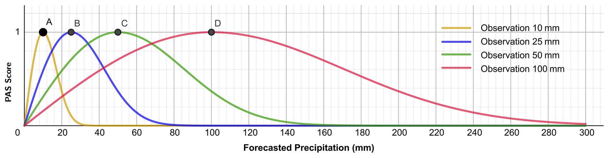
Figure 1 Schematic diagram of the precipitation accuracy score (PAS) curves when the observed precipitation amounts are 10, 25, 50, and 100 mm.

2 Cross-scale general comprehensive evaluation method

2.1 Overview of the general comprehensive evaluation method

To address the issues of “distorted scores due to the division of precipitation thresholds and increased subjective risks brought about by the setting of the neighborhood spatial verification method” in traditional and improved precipitation scoring methods, this study refers to the verification method for heavy-rainfall forecasts based on predictability (Chen et al., 2019) and combines the advantages of relative and absolute errors. A GCEM is constructed by directly analyzing the proximity of forecasted precipitation to observed precipitation. It primarily includes the PAS, and the expression of its core scoring function is as follows:

$$\begin{array}{}\text{(1)}& \mathrm{PAS}=\left\{\begin{array}{ll}\sin \left(\frac{\mathit{\pi }}{\mathrm{2}}\cdot \frac{x}{u}\right),& \mathrm{0}\le x<u\\ e^{-{\left(\frac{x-u}{u}\right)}^{\mathrm{2}}},& \mathrm{0}<u\le x,\end{array}\right.\end{array}$$

where PAS represents the scoring value, x is the forecasted precipitation (mm), and u is the observed precipitation (mm). The PAS falls between 0 and 1, where a higher score indicates a better precipitation forecast effect. When PAS = 1, it signifies a perfect forecast, indicating that the forecasted and observed precipitation match entirely. For Eq. (1), given the observation value u>0 mm, when the forecasted precipitation is 0 mm, then PAS = 0, indicating that the model has no forecast skill. When the forecasted precipitation amount is sufficiently large, PAS → 0, indicating no forecast skill as well (Fig. 1). Additionally, considering the large fluctuation characteristics of the function curve when the observed precipitation is less than 10 mm, Eq. (1) was smoothed and optimized (see Sect. 2.2 for details).

The GCEM system also includes the following indices:

1. An insufficient precipitation index (IPI), whose core scoring function expression is as follows:

   $$\begin{array}{}\text{(2)}& \mathrm{IPI}=\sin \left({\displaystyle \frac{\mathit{\pi }}{\mathrm{2}}}\cdot {\displaystyle \frac{x}{u}}\right)-\mathrm{1},\mathrm{0}\le x<u,\end{array}$$

   where IPI represents the scoring value, reflecting the degree of underestimation in precipitation forecasts when the forecasted value is less than the observed value. The IPI falls within [−1, 0), where a value closer to 0 indicates a lower degree of underestimation.

2. An excessive precipitation index (EPI), whose core scoring function expression is as follows:

   $$\begin{array}{}\text{(3)}& \mathrm{EPI}=\mathrm{1}-e^{-{\left(\frac{x-u}{u}\right)}^{\mathrm{2}}},\mathrm{0}<u<x,\end{array}$$

   where EPI represents the scoring value, reflecting the degree of overestimation in precipitation forecasts when the forecasted value exceeds the observed value. The EPI falls within (0, 1), where a value closer to 0 indicates a lower degree of overestimation.

3. An insufficient and excessive precipitation index (IEPI), whose core scoring function expression is as follows:

   $$\begin{array}{}\text{(4)}& \mathrm{IEPI}=\left\{\begin{array}{ll}\sin \left(\frac{\mathit{\pi }}{\mathrm{2}}\cdot \frac{x}{u}\right)-\mathrm{1},& \mathrm{0}\le x<u\\ \mathrm{1}-e^{-{\left(\frac{x-u}{u}\right)}^{\mathrm{2}}},& \mathrm{0}<u\le x,\end{array}\right.\end{array}$$

   where IEPI represents the scoring value, reflecting the degree of deviation of the forecasted precipitation from the observed precipitation. The IEPI falls within [−1, 1), where a value closer to 0 indicates a lower degree of forecast deviation. An IEPI less (more) than 0 indicates an insufficient (excessive) forecast, and an IEPI equal to 0 represents an unbiased forecast.

   Additional explanation is as follows: Eqs. (2)–(4) are a series of theoretical indicator formulas derived from Eq. (1); therefore, Eqs. (2)–(4) are referred as the core calculation formulas for the IPI, EPI, and IEPI, respectively. In practical applications, the optimized solution will be used (see Sect. 2.2) to calculate the IPI, EPI, and IEPI for the situations of u≥0.1 mm or x≥0.1 mm.

4. A PAS clear/rainy forecast accuracy score (PASC), whose scoring function expression is as follows:

   $$\begin{array}{}\text{(5)}& \mathrm{PASC}=\left\{\begin{array}{ll}\mathrm{1}& \mathrm{0}\le u<\mathrm{0.1}\text{ and }\mathrm{0}\le x<\mathrm{0.1}\\ {\mathrm{PAS}}_{\mathrm{|}ux\mathrm{0.1}}& u\ge \mathrm{0.1}\text{ or }x\ge \mathrm{0.1},\end{array}\right.\end{array}$$

   where PASC represents the PAS scoring value for clear/rainy forecasts. “$\mathrm{0}\le u<\mathrm{0.1}$ and $\mathrm{0}\le x<\mathrm{0.1}$” denotes the correctly forecasted non-precipitation event with PASC = 1. PAS_|ux0.1 denotes the overall PAS for precipitation forecasts under specific conditions where the observed precipitation u≥0.1 mm or the forecasted precipitation x≥0.1 mm.

The discussion below pertains to the characteristics of the PAS scoring method. As an ideal performance indicator, the PAS has the attributes of boundedness, fairness, sensitivity disparity, suitability for extreme events, and moderate symmetry.

1. Boundedness. The PAS scoring values range between 0 and 1. A PAS score of 1 represents an ideal forecast, while a score of 0 indicates that there is observed precipitation but no forecasted precipitation or that the forecasted precipitation is sufficiently large. The scoring range is consistent with that of traditional TS, making it easy to compare and evaluate the scoring methods and suitable for practical forecast verification applications.

2. Fairness. The PAS scoring method constitutes a scoring formula in an objective form without a subjective boundary definition. Precipitation forecasts are verified without magnitude or delimitation of the area of influence, and the closer to the observed situation the forecast is, the higher the score will be, which is fair.

3. Sensitivity disparity. According to the Chinese national standard GB/T 28592–2012 grade of precipitation on the classification of precipitation grades, the public is more sensitive to low-grade precipitation forecasts. As the rainfall intensity increases, so too will the public's sensitivity gradually decrease; that is, the public has a higher tolerance for errors in response to heavier-rainfall forecasts. In other words, large errors in the forecasts of heavy-rainfall events may be considered equivalent to smaller errors in weaker-rainfall events in terms of forecast scoring. As shown in Fig. 1, the intersection point on the PAS scoring curves for the observed precipitation amounts of 25 and 100 mm corresponds to a forecasted amount of 42.4 mm. That is, the forecast errors are 17.4 and 57.6 mm for the observed 24 h accumulated precipitation amounts of 25 and 100 mm, respectively, while the scores are both 0.62. From the perspective of forecast service effectiveness, this aligns with general public perception.

4. Suitability for extreme events. From the PAS scoring curves for forecasts corresponding to different observed precipitation amounts (u=10, 25, 50, and 100 mm) (Fig. 1), it is evident that the PAS scoring method performs well in evaluating precipitation event forecasts at the level of torrential rain and above. For example, when the observed precipitation is 100 mm, with forecasted amounts of 59 and 147.2 mm, the PASs are both 0.8, whereas the TSs are 0 and 1, and the improved TSs are 0.8 and 1, respectively. This result indicates that the PAS is suitable for scoring heavy-rainfall events, meeting the general applicability requirements as a scoring method that does not degrade due to extreme events.

5. Moderate symmetry. In Eq. (1), let the observed precipitation be the independent variable u and the forecasted precipitation be the parameter x. Similarly, for different magnitudes of forecasted precipitation (parameter x=10, 25, 50, and 100 mm) and observed precipitation (variable u) ranging from 0 to 300 mm, the corresponding scores are shown in Fig. 2. The scores also vary with the degree of proximity between forecasts and observations. Figures 1 and 2 exhibit similar trends but are not identical, illustrating that the PAS possesses moderate symmetry.

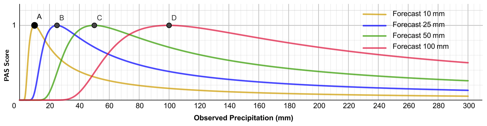
Figure 2 PAS curves corresponding to different forecasted precipitation amounts (10, 25, 50, and 100 mm).

2.2 PAS verification for precipitation forecasts

From the properties of the core verification function of the PAS, it is noted that when the observed precipitation u<10 mm, there is a large gradient in the PAS curve. A slight change in the forecasted value (x) can result in a large fluctuation in the PAS. To account for this characteristic, based on a comprehensive analysis in combination with the sensitivity of forecasters and the public to small-scale precipitation, a smoothing optimization scheme is applied to the PAS curve for accumulated precipitation below 10 mm. Similarly, the IPI, EPI, IEPI, and PASC curves are appropriately smoothed and optimized according to their respective definitions.

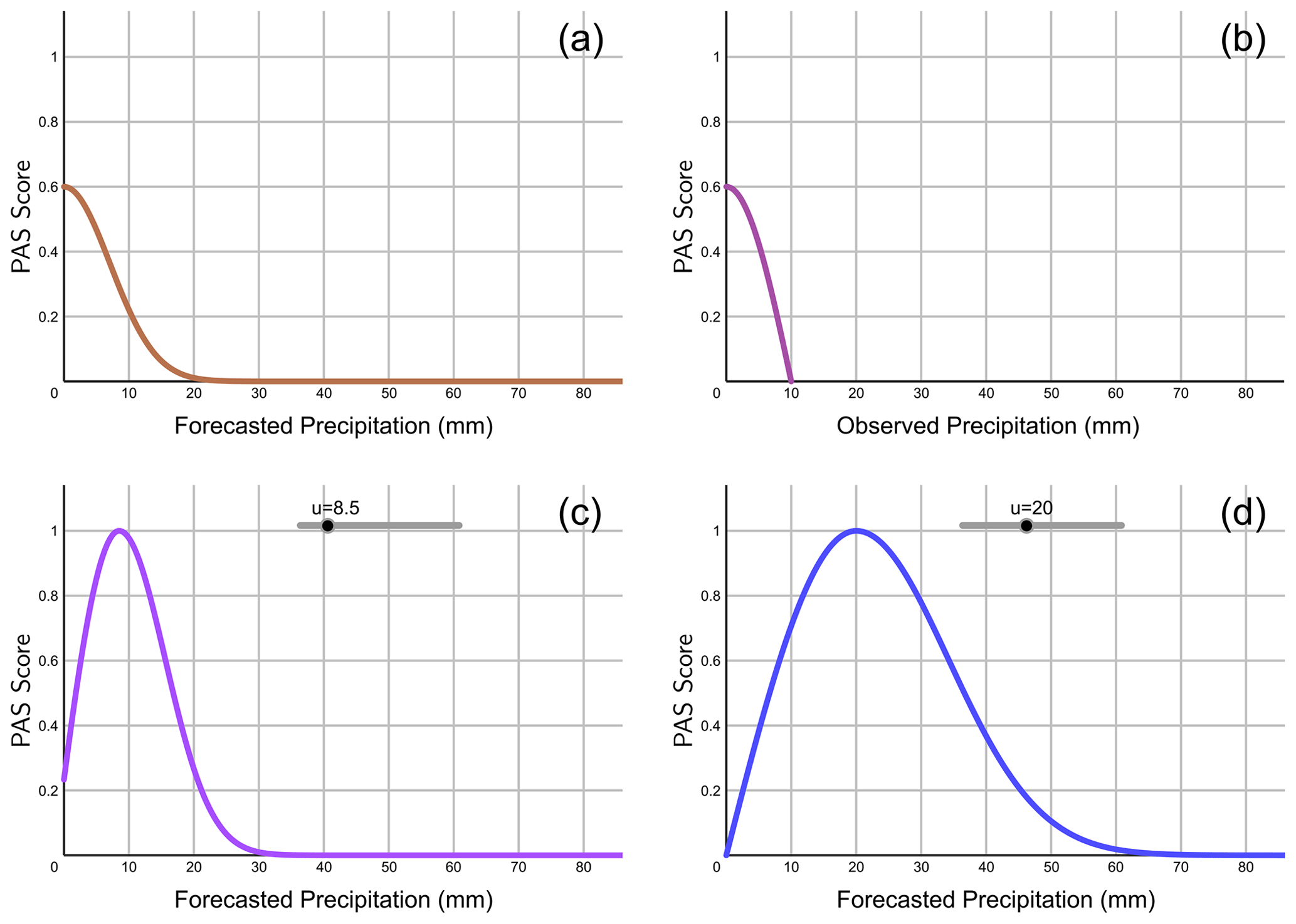
Figure 3 PAS curves of precipitation forecasts when (a) the observed precipitation u=0 mm and the forecasted precipitation x>0 mm, (b) the observed precipitation $\mathrm{0}<u<\mathrm{10}$ mm and the forecasted precipitation x=0 mm (the horizontal coordinate denotes the observed precipitation u), (c) the observed precipitation $\mathrm{0}<u<\mathrm{10}$ mm and the forecasted precipitation x>0 mm, and (d) the observed precipitation u≥10 mm.

The assumptions are as follows:

• 1.

  $\mathrm{PAS}=\mathrm{0.6}{\mathrm{PAS}}_{\mathrm{|}u\to \mathrm{0}}$ when u=0 mm and x≠0 mm; PAS_|u→0 denotes the PAS for the case of the observed precipitation at $\mathrm{0}<u\le \mathrm{0.1}$ mm.

• 2.

  $\mathrm{PAS}=\mathrm{0.6}{\mathrm{PAS}}_{\mathrm{|}x\to \mathrm{0}}$ when x=0 mm and $\mathrm{0}<u<\mathrm{10}$ mm; PAS_|x→0 denotes the PAS for the case of the forecasted precipitation at $\mathrm{0}<x\le \mathrm{0.1}$ mm.

• (a)

  When the observed precipitation is u=0 mm, and the forecasted precipitation is x>0 mm (Fig. 3a), let $\mathrm{PAS}=\mathrm{0.6}{\mathrm{PAS}}_{\mathrm{|}u\to \mathrm{0}}$, and then

  $$\begin{array}{}\text{(6)}& \mathrm{PAS}=\mathrm{0.6}{e}^{-{\left(\frac{x}{\mathrm{10}}\right)}^{\mathrm{2}}}x>\mathrm{0}.\end{array}$$
• (b)

  When the forecasted precipitation is x=0 mm, and the observed precipitation is $\mathrm{0}<u<\mathrm{10}$ mm (Fig. 3b), let $\mathrm{PAS}=\mathrm{0.6}{\mathrm{PAS}}_{\mathrm{|}x\to \mathrm{0}}$, and then

  $$\begin{array}{}\text{(7)}& \mathrm{PAS}=\begin{array}{l}\mathrm{0.6}\sin \left(\frac{\mathit{\pi }}{\mathrm{2}}\cdot \frac{\mathrm{10}-u}{\mathrm{10}}\right),\mathrm{0}<u<\mathrm{10}.\end{array}\end{array}$$

  The coefficient was set to 0.6. According to Eqs. (6)–(7), when the situation is the observation with u=0 mm and forecast with x=0.1 mm or the observation is u=0.1 mm and forecast is x=0 mm, then PAS = 0.6, suggesting that the forecast effect has just reached the standard, like when the ACC reaches 0.6, which indicates that the model forecast effect is available (Zhao and Zhang, 2018).

• (c)

  When the observed precipitation is $\mathrm{0}<u<\mathrm{10}$ mm, and the forecasted precipitation is x≠0 (Fig. 3c), then

  $$\begin{array}{}\text{(8)}& \mathrm{PAS}=\left\{\begin{array}{lll}\sin \left(\frac{\mathit{\pi }}{\mathrm{2}}\cdot \frac{x-u+\mathrm{10}}{\mathrm{10}}\right),& \mathrm{0}<x<u,& \mathrm{0}<u<\mathrm{10},\\ e^{-{\left(\frac{x-u}{\mathrm{10}}\right)}^{\mathrm{2}}},& u\le x,& \mathrm{0}<u<\mathrm{10}.\end{array}\right.\end{array}$$
• (d)

  When the observed precipitation is u≥10 mm (Fig. 3d), then

  $$\begin{array}{}\text{(9)}& \mathrm{PAS}=\left\{\begin{array}{lll}\sin \left(\frac{\mathit{\pi }}{\mathrm{2}}\cdot \frac{x}{u}\right),& \mathrm{0}\le x<u,& u\ge \mathrm{10},\\ e^{-{\left(\frac{x-u}{u}\right)}^{\mathrm{2}}},& u\le x,& u\ge \mathrm{10}.\end{array}\right.\end{array}$$

  To compare with the traditional scoring method, the new scoring method for precipitation forecasting adopts the “classification before verification, no classification during verification” approach. Scoring for precipitation processes over different accumulation periods is referenced but not limited to the commonly used precipitation classification approaches in practical operations, as shown in Tables 3–5.

Table 3 Classification of PAS for short-term heavy rainfall.

Table 4 Classification of PAS for 12 h accumulated precipitation.

Table 5 Classification of PAS for 24 h accumulated precipitation.

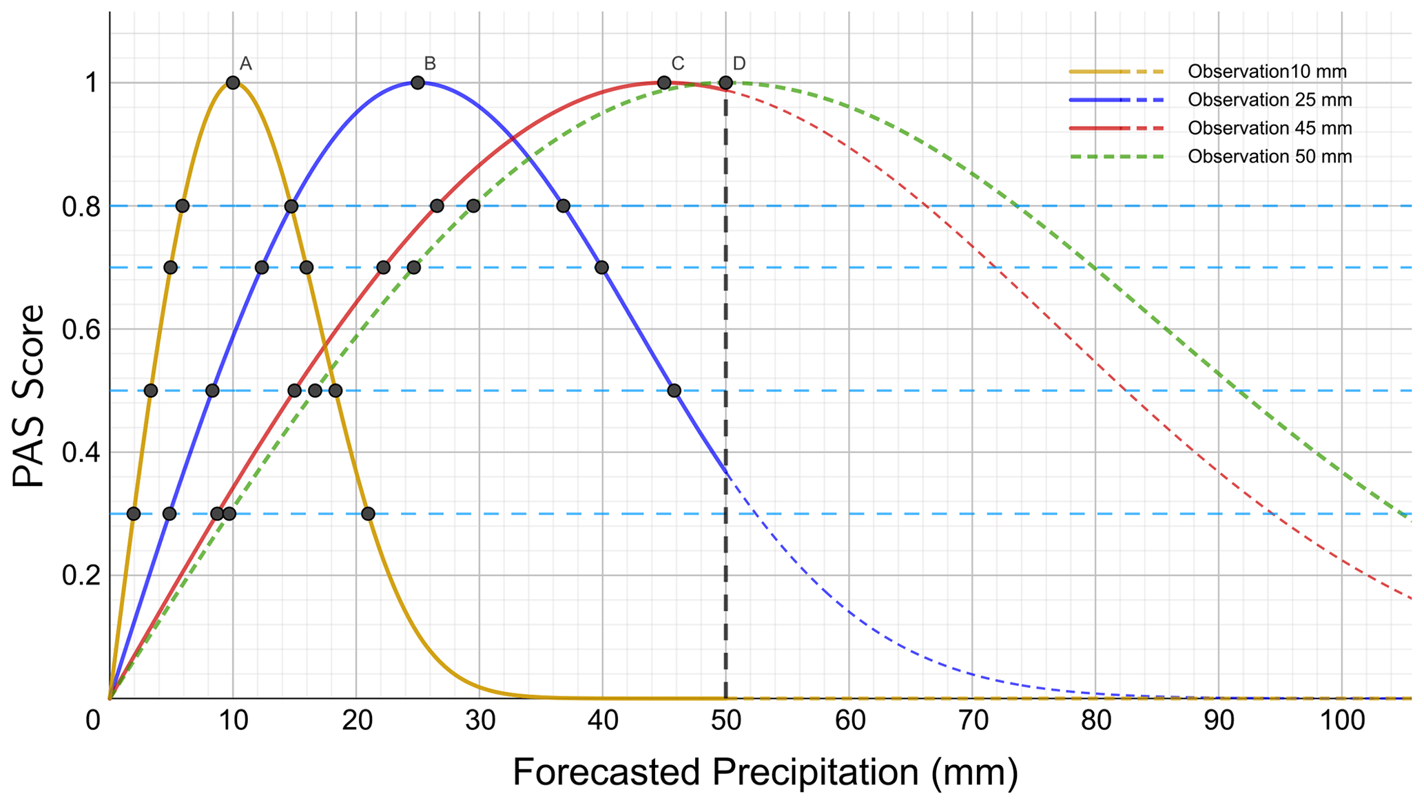
Figure 4 PAS curves of the forecasts under general precipitation conditions (u=10, 25, and 45 mm). The solid line part of the curve in the figure is involved in the comparison. The dashed line part is not involved in the comparison. The 10 mm observed precipitation is represented by the orange line, the 25 mm observed precipitation is represented by the blue line, the 45 mm observed precipitation is represented by the red line, and the 50 mm observed precipitation is represented by the green line.

Table 6 Examples of forecast verification scores for general precipitation (u=25, 50, and 100 mm).

3 Ideal experimental validation of the new verification method

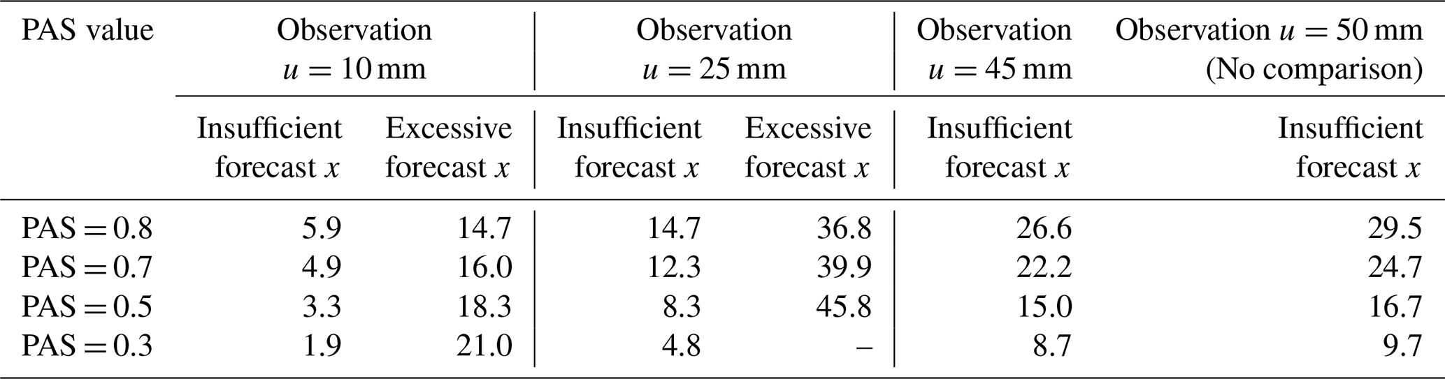
3.1 Validation of forecast scoring results for general precipitation

General precipitation refers to precipitation ranging from light rain to heavy rain, i.e., 24 h accumulated precipitation within [0.1, 50 mm). Figure 4 shows the schematic diagram of PAS scores for general precipitation. The forecasted amounts are compared under conditions when the 24 h accumulated precipitation is 10, 25, and 45 mm and the PAS scores are 0.8, 0.7, 0.5, and 0.3 (Table 6). When the observed precipitation is 10 mm, the forecasted amounts of 5.9 and 14.7 mm both have a PAS score of 0.8, with differences from the perfect forecast value (10 mm) of 4.1 and 4.7 mm, respectively; the forecasted amounts with a PAS score of 0.3 are 1.9 and 21.0 mm, differing by 8.1 and 11.0 mm from the perfect forecast value (10 mm), respectively. When the observed precipitation is 25 mm, the forecasted amounts with a PAS score of 0.8 are 14.7 and 36.8 mm, with differences from the perfect forecast value (25 mm) of 10.3 and 11.8 mm, respectively; the forecasts with a PAS score of 0.5 are 8.3 and 45.8 mm, differing by 16.7 and 20.8 mm from the perfect forecast value (25 mm), respectively.

For forecasts with the same observed precipitation and the same scores, the absolute errors in an insufficient forecast and observation are smaller than those of an excessive forecast and observation, and the higher the scores are, the closer the absolute errors in the forecasts will be. When the observed precipitation is 50 mm, only the insufficient precipitation forecast is scored since a precipitation forecast exceeding 50 mm is not considered within the scope of general precipitation evaluation. The scoring experimental results align with expectations.

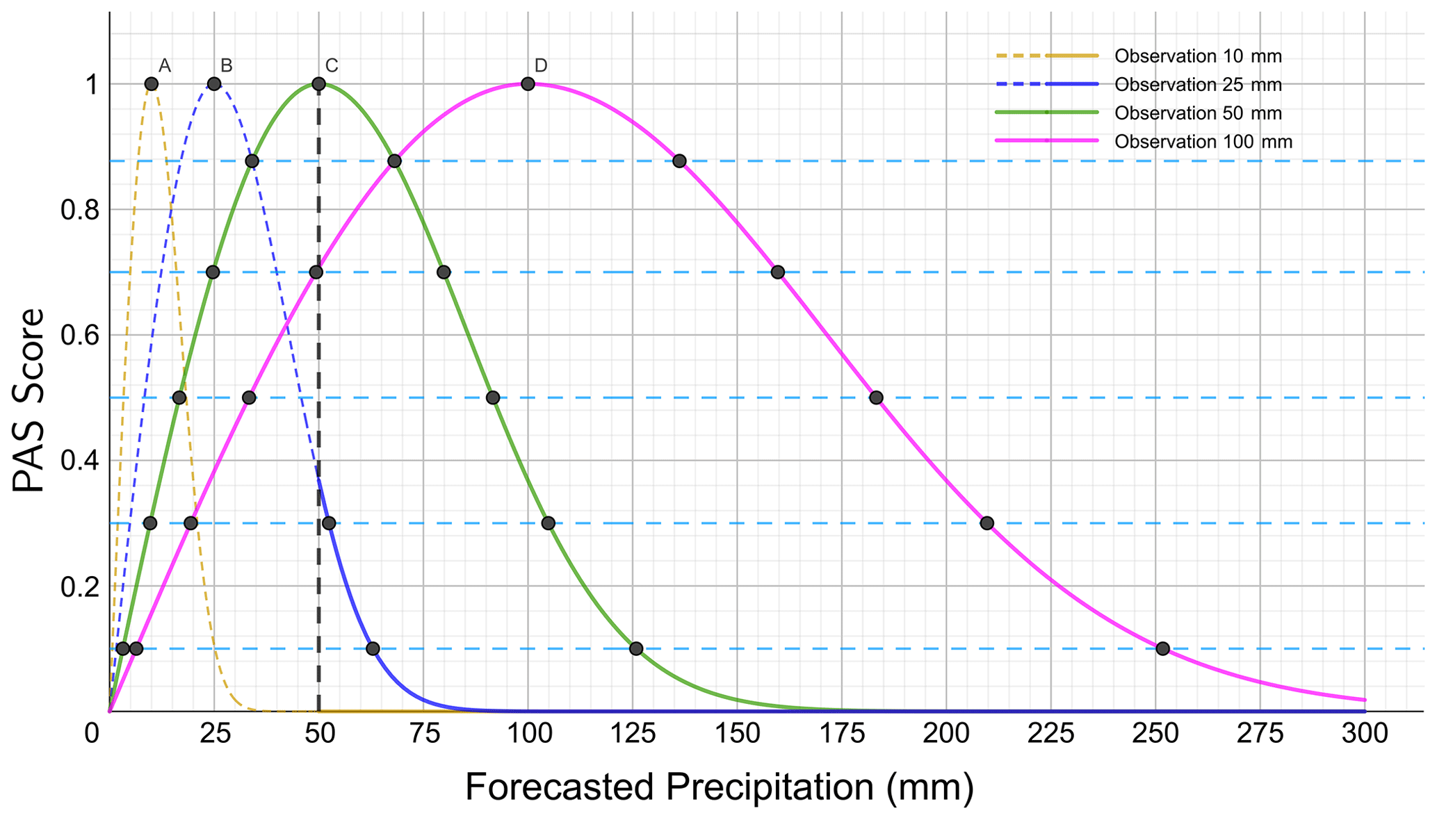
Figure 5 Same as Fig. 4 but for precipitation at the level of torrential rain and above (u=25, 50, and 100 mm). The solid line part of the curve in the figure is involved in the comparison. The dashed line part is not involved in the comparison. The 10 mm observed precipitation is represented by the orange line, the 25 mm observed precipitation is represented by the blue line, the 50 mm observed precipitation is represented by the green line, and the 100 mm observed precipitation is represented by the red line.

Table 7 Same as Table 6 but for precipitation at the level of torrential rain and above (u=25, 50, and 100 mm).

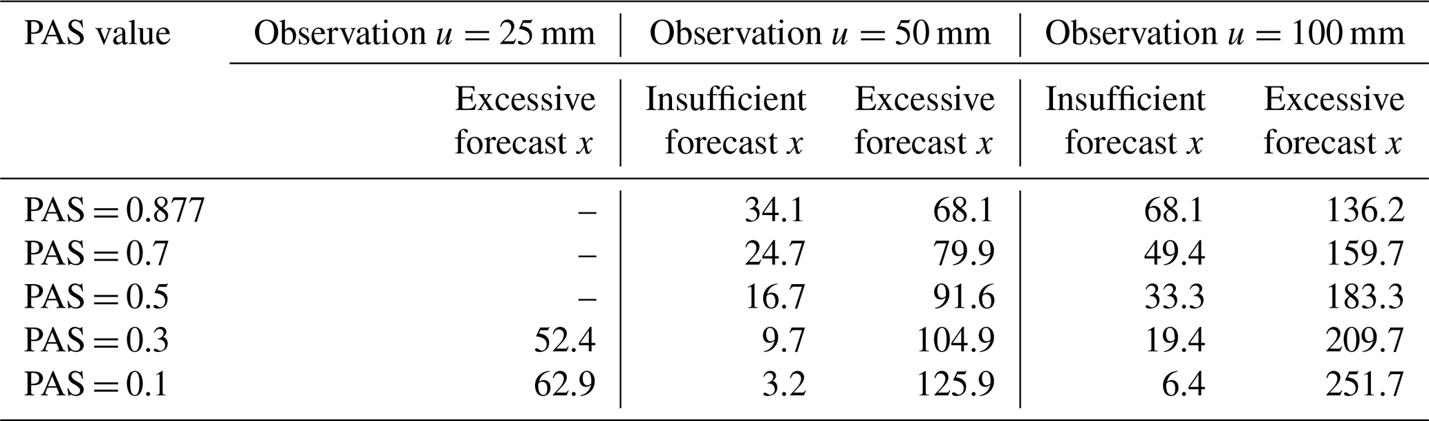
3.2 Validation of forecast scoring results for precipitation at the level of torrential rain and above

Figure 5 shows a schematic diagram of the PASs when the amount of precipitation exceeds the storm magnitude. The predicted precipitation is compared when the 24 h cumulative observed precipitation is 25, 50, and 100 mm with PAS scores of 0.877, 0.7, 0.5, 0.3, and 0.1 (Table 7). When the observed precipitation is 25 mm, only forecasts of ≥50 mm are involved in the rating, with PASs of 0.3 and 0.1 for forecasts of 52.4 and 62.9 mm, respectively.

When the PAS is 0.877 and the observed precipitation is 50 mm, the predicted values are 34.1 and 68.1 mm, respectively; when the observed precipitation is 100 mm, the predicted values are 68.1 and 136.2 mm, respectively. When the observed precipitation is 50 or 100 mm, the prediction is 68.1 mm, with a score of 0.877. The absolute error is 18.1 mm for the excessive precipitation forecast and 31.9 mm for the insufficient precipitation forecast. This result indicates that the scoring tolerance increases as the grade of observed precipitation increases and gradually expands through continuous changes, avoiding discontinuous increases caused by changes in magnitude.

When the observed precipitation is 50 mm and the PAS is 0.3, the insufficient forecast is 9.7 mm, and the excessive forecast is 104.9 mm. When the observed precipitation is 100 mm, the predictions for a PAS of 0.3 are 19.4 and 209.7 mm, respectively. When the observed precipitation is 50 mm, the insufficient forecast with a PAS of 0.1 is 3.2 mm, and the excessive forecast is 125.9 mm. When the observed precipitation is 100 mm, the predictions with a PAS of 0.1 are 6.1 and 251.7 mm, respectively.

Under constant observed precipitation conditions for forecasts with the same score, the absolute error between the insufficient forecast and the observed precipitation is smaller than that between the excessive forecast and the observed precipitation. The higher the score is, the smaller the absolute error between the forecast and the observation will be. Moreover, the scoring tolerance increases with increasing observed precipitation. The scoring experimental results conform to expectations.

4 Example-based comparative experiments for the new verification method

Different examples are selected for the new precipitation verification method, and its multifaceted characteristics are demonstrated through comparative experiments. In Sect. 4.1, two typical cases are selected, the performance characteristics of the PAS and TS are compared, and the indicators of insufficient and excessive forecasts and spatial verification in the GCEM are analyzed. In Sect. 4.2, a typical case of extreme-precipitation event is selected, and the forecast results of different high-resolution models using the PAS, TS, and FSS methods are evaluated to verify the advantages and characteristics of the new precipitation verification method for extreme-precipitation events.

4.1 Comparative experiments of two typical processes

4.1.1 Introduction of typical cases

Comparative experiments of PAS and traditional TS are conducted for 12 h accumulated precipitation for two typical cases. One case pertains to the precipitation weather process occurring during 00:00 to 12:00 UTC on 16 July 2019 (referred to as “Case 1”), which is dominated by a weak weather system. The other case relates to the precipitation weather process occurring during 00:00 to 12:00 UTC on 13 June 2020 (referred to as “Case 2”), which is predominantly associated with a strong weather system.

Both precipitation cases are associated with precipitation during the Meiyu period. Case 1 occurred during the Meiyu period of 2019 and was characterized by scattered precipitation under weak synoptic-scale forcing. The low-intensity shear line system is located south of the Yangtze River. There are two precipitation concentration areas: one at the intersection of Hunan province and Jiangxi province and the other covering the majority of Zhejiang province. The precipitation process in Case 2 (12–13 June) was the first round of widespread rainstorms during the Meiyu period of 2020, including heavy precipitation affected by a low-level vortex shear system. The western section of the low-level vortex shear is relatively stable, while the eastern section slightly presses southwards. Southwesterly airflow developed and pushed northwards, and a strong wind speed belt persisted for a long time in the Jianghuai region. Moreover, the Jianghan–Jianghuai region maintained a high-energy and high-moisture state, resulting in persistent heavy rainfall.

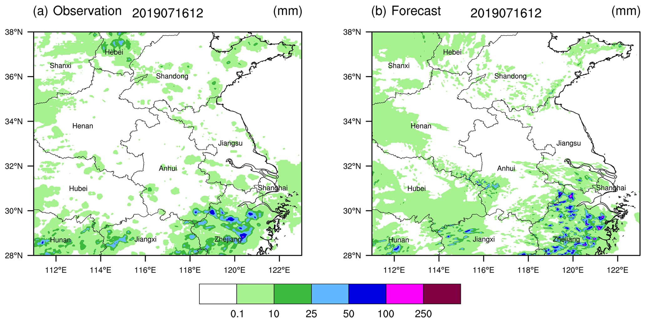
Figure 6 Accumulated precipitation (a) observed and (b) forecasted from 00:00 to 12:00 UTC on 16 July 2019.

A subjective analysis of these two weather processes reveals that for the event on 16 July 2019 (Fig. 6), the forecasted precipitation intensity and rainfall areas are relatively consistent with the observations. There are two distinct heavy-rainfall areas in the eastern and southern parts of the Yangtze River, with particularly high accuracy in forecasting scattered rainstorms in Zhejiang province located in the eastern section. In contrast, for the precipitation weather process on 13 June 2020 (Fig. 7), it is evident that there is an overestimation of the precipitation forecast.

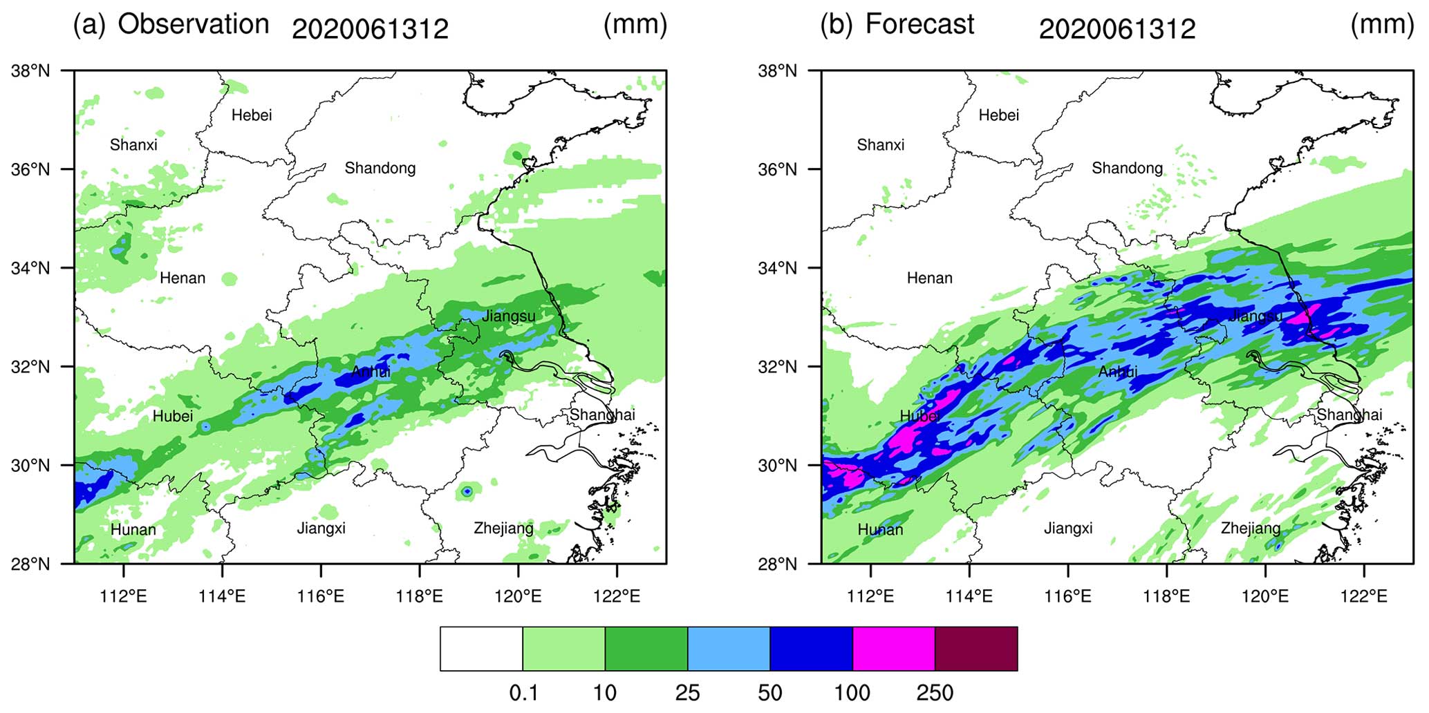
Figure 7 Accumulated precipitation (a) observed and (b) forecasted from 00:00 to 12:00 UTC on 13 June 2020.

4.1.2 Data and methods

The observed precipitation data are provided by the China Meteorological Administration multi-source merged precipitation analysis system (CMPAS), as developed by the National Meteorological Information Centre of China. The CMPAS integrates hourly precipitation data from nearly 40 000 automatic meteorological stations in China and provides radar-based quantitative precipitation estimation and satellite-retrieved precipitation products with a spatial resolution of 0.05° × 0.05°. The predicted precipitation data with 3 km resolution are from the Precision Weather Analysis and Forecasting System (PWAFS) model, a regionally refined forecast model, developed by the Jiangsu Provincial Meteorological Bureau. These data are output once per hour.

The specific methods are as follows.

1. Determine the verification domain and verification points. The verification domain covers the Huang–Huai region of China (28–38° N, 111–123° E). The verification points are defined based on the grid points of the observed precipitation data; their spatial resolution is 0.05° × 0.05°, and the total number of verification grid points is 48 000 (200×240).

2. Prepare the observed and forecasted precipitation data and interpolate the forecasted precipitation data onto the observed grid points. The observed 12 h accumulated precipitation data are derived by accumulating the hourly precipitation data from the CMPAS. The forecasted 12 h accumulated precipitation data are obtained by subtracting the zero-field data from the 12 h forecast field data. Since the grid points of the observed and forecasted precipitation data do not coincide, and the grid spacing is small, the nearest-neighbor method is used in this study to match the forecasted data to the grid points of the observed precipitation. Specifically, the forecasted data on the model grid nearest to the observed grid are used as the forecasted value at this observed grid.

3. Analyze the relationship between the forecasted precipitation and observed precipitation. The scores for each verification grid point and the overall scores for each verification area are calculated based on the scoring formula for each index in the GCEM system. Then, the verification result file is generated in NetCDF format. On this basis, distribution maps for the scores of various indices in the GCEM system are produced. Additionally, the total TS and clear/rainy TS for different precipitation magnitudes within the verification area is calculated based on the TS and clear/rainy TS formulas.

Table 8 PAS and TS of 12 h accumulated precipitation from 00:00 to 12:00 UTC on 16 July 2019.

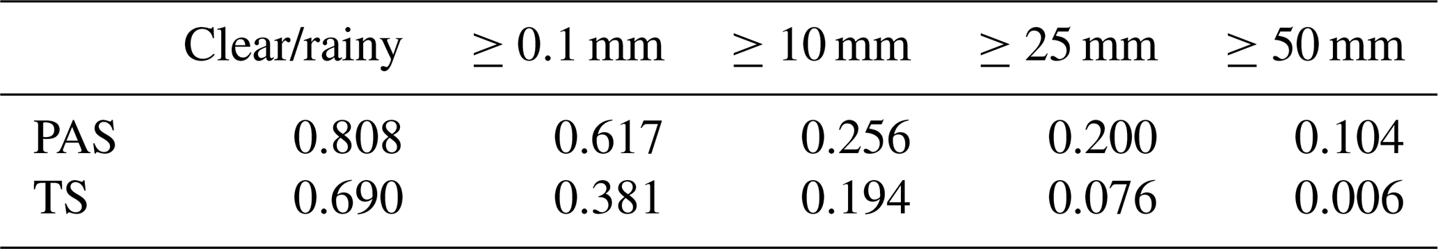
Table 9 Same as Table 8 but from 00:00 to 12:00 UTC on 13 June 2020.

4.1.3 Analysis of the comparative experiment results

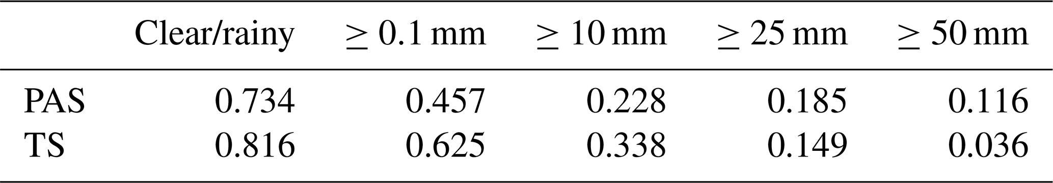
For the precipitation process on 16 July 2019, the traditional TSs for different rainfall categories, such as clear/rainy and 12 h accumulated precipitation of ≥0.1, ≥10 mm, ≥25, and ≥50 mm are all lower than the traditional TSs for the weather process on 13 June 2020. For example, the TS is 0.381 for 12 h accumulated precipitation of ≥0.1 mm during 00:00 to 12:00 UTC on 16 July 2019 (Table 8), while this score is 0.625 for that during 00:00 to 12:00 UTC on 13 June 2020 (Table 9), which differs from the subjective judgment.

For the precipitation process during 00:00 to 12:00 UTC on 16 July 2019, the PASs for clear/rainy and 12 h accumulated precipitation of ≥0.1, ≥10, and ≥25 mm are all higher than those for the precipitation process during 00:00 to 12:00 UTC on 13 June 2020. For instance, the overall PAS is 0.617 for 12 h accumulated precipitation of ≥0.1 mm during 00:00 to 12:00 UTC on 16 July 2019. This PAS is higher than the PAS of 0.457 for the precipitation process during 00:00 to 12:00 UTC on 13 June 2020, which aligns with the subjective judgment.

For the precipitation process during 00:00 to 12:00 UTC on 16 July 2019, the PAS for each magnitude is higher than the corresponding TS, thereby addressing the issue of TSs being lower. For the precipitation process during 00:00 to 12:00 UTC on 13 June 2020, the PASs for clear/rainy and the magnitudes of ≥0.1 and ≥10 mm are lower than the corresponding TSs, whereas the PASs for the magnitudes of ≥25 and ≥50 mm are higher than the corresponding TSs. This result indicates that the PAS is different from the magnitude-improved TS and the neighborhood spatial verification method. Both the magnitude-improved TS and the neighborhood spatial verification method increase the tolerance, leading to a monotonous increase in scores. This result also demonstrates that the PAS has good discrimination ability for extreme events. The PAS assigns scores based on the proximity of the forecast to the observation, making it more reliable for precipitation evaluation than the TS.

4.1.4 Analysis of the indices in the new verification method

Modern forecast verification is based mainly on spatial verification methods to compensate for the shortcomings of traditional methods. The literature review of Gilleland et al. (2009) defines four main categories of the methods: neighborhood, scale separation, features-based, and field deformation (Ahijevych et al., 2009). These methods can analyze more comprehensively in specific individual cases but seem to be less able to provide direct overall scoring results than traditional scoring methods in the statistics of long time series. GCEM is based on point-to-point scoring statistics without a radius of influence, no isolation of features at each scale, and no definition of objects in the forecast and observation to analyze the similarity of the objects or to fit the forecast objects through deformation operations. However, the GCEM still has spatial attributes that can discriminate spatial forecast characteristics (e.g., insufficient or excessive forecasting scenarios) for different categories of precipitation, and the GCEM can carry out statistical verification of long time series and produce overall scoring results.

Regarding the issue of analyzing the sources of errors from the verification results, objectively tracing these errors back from a single score can only determine whether an error was “insufficient” (missed alarm) or “excessive” (false alarm). However, the advantage of the GCEM lies in its ability to decompose the score for each verification point and examine the forecasting performance at each point, which is different from the dichotomous evaluation approach with only 0 and 1 outputs. These indices not only provide overall scores for individual cases similar to the TS but also offer two-dimensional score distribution plots which can comprehensively reflect the performance and characteristics of precipitation forecasts.

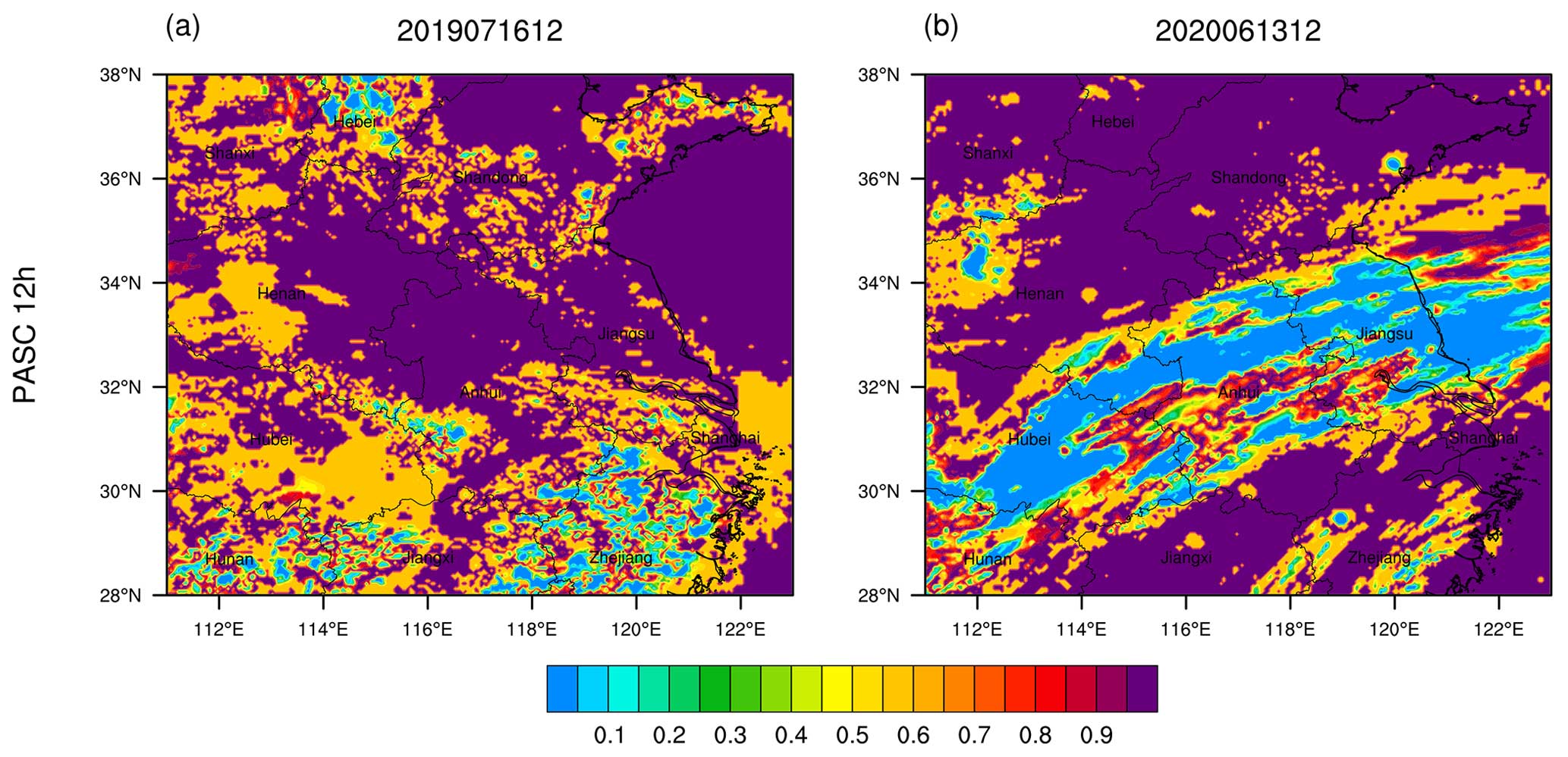
Figure 8 Distributions of the PAS clear/rainy forecast accuracy score (PASC) of 12 h accumulated precipitation for (a) Case 1 from 00:00 to 12:00 UTC on 16 July 2019 and (b) Case 2 from 00:00 to 12:00 UTC on 13 June 2020.

Figure 8 shows the distributions of the 12 h accumulated precipitation PASC scores. In these two cases, due to the high accuracy of non-precipitation forecasts, the overall PASC scores are relatively high. However, for Case 1, the scores in Zhejiang are lower and scattered within a small area. In contrast, for Case 2, there is a large area occupying most of the Jianghuai region with low scores. Therefore, the PASC score of Case 1 (0.808) is higher than that of Case 2 (0.734).

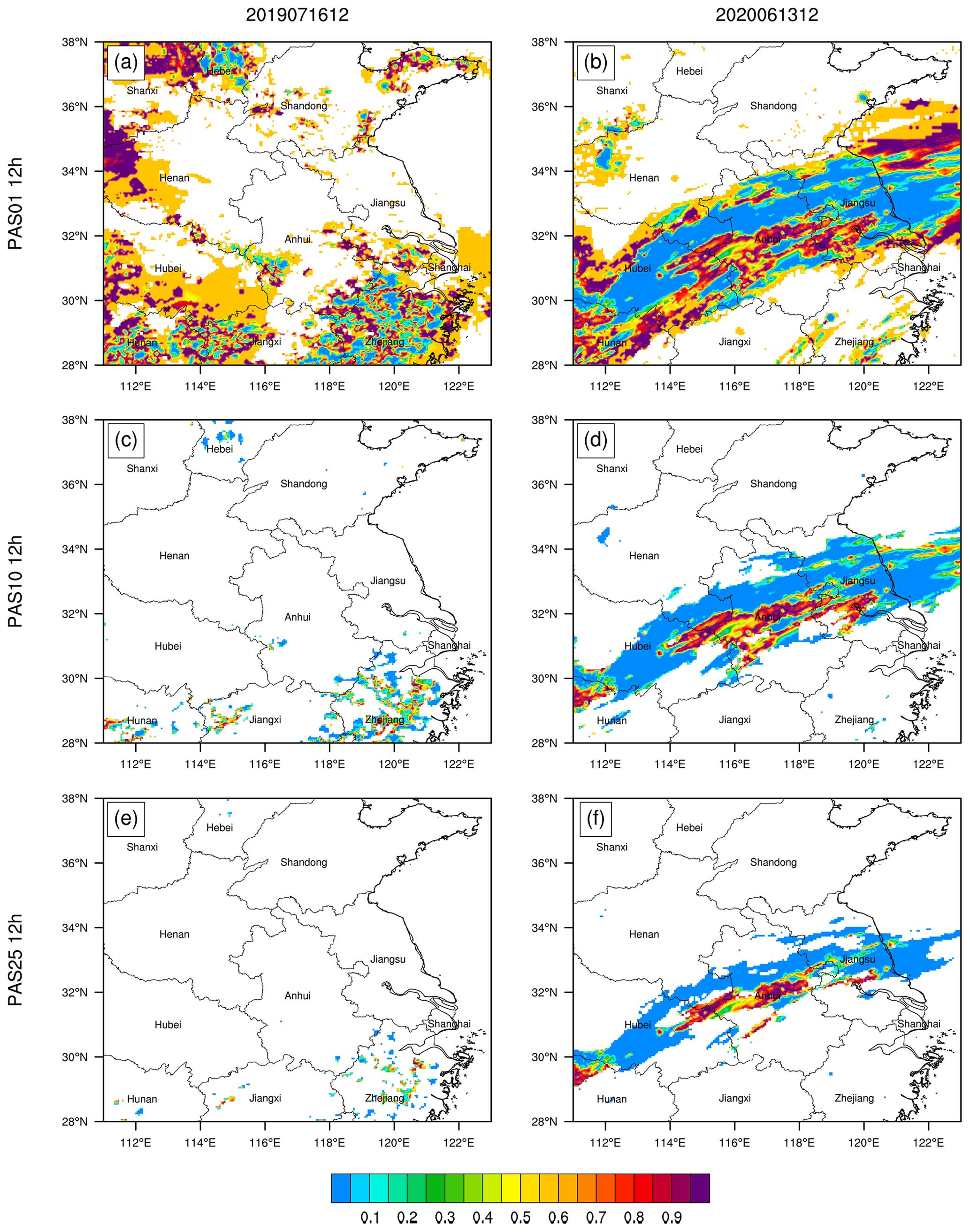
Figure 9 Distributions of PAS of 12 h accumulated precipitation of ≥0.1 mm for (a) Case 1 from 00:00 to 12:00 UTC on 16 July 2019 and (b) Case 2 from 00:00 to 12:00 UTC on 13 June 2020, of ≥10 mm for (c) Case 1 and (d) Case 2, and of ≥25 mm for (e) Case 1 and (f) Case 2.

Figure 9 shows the PAS distributions of 12 h accumulated precipitation with magnitudes of ≥0.1, ≥10, and ≥25 mm. The blank points in the figure are the points that are excluded in the scoring, following the scoring principle of “classification before verification, no classification during verification” described in Sect. 2. From the PAS distributions of different magnitudes, for Case 1, the high and low scores in the Zhejiang region are scattered among them. In contrast, for Case 2, the scoring areas in the Jianghuai region have a larger area of low scores than high scores. Therefore, Case 1 has higher PASs for the three categories (≥0.1, ≥10, and ≥25 mm) than Case 2, and the distributions also allow distinguishing the areas with better and worse forecasting performance.

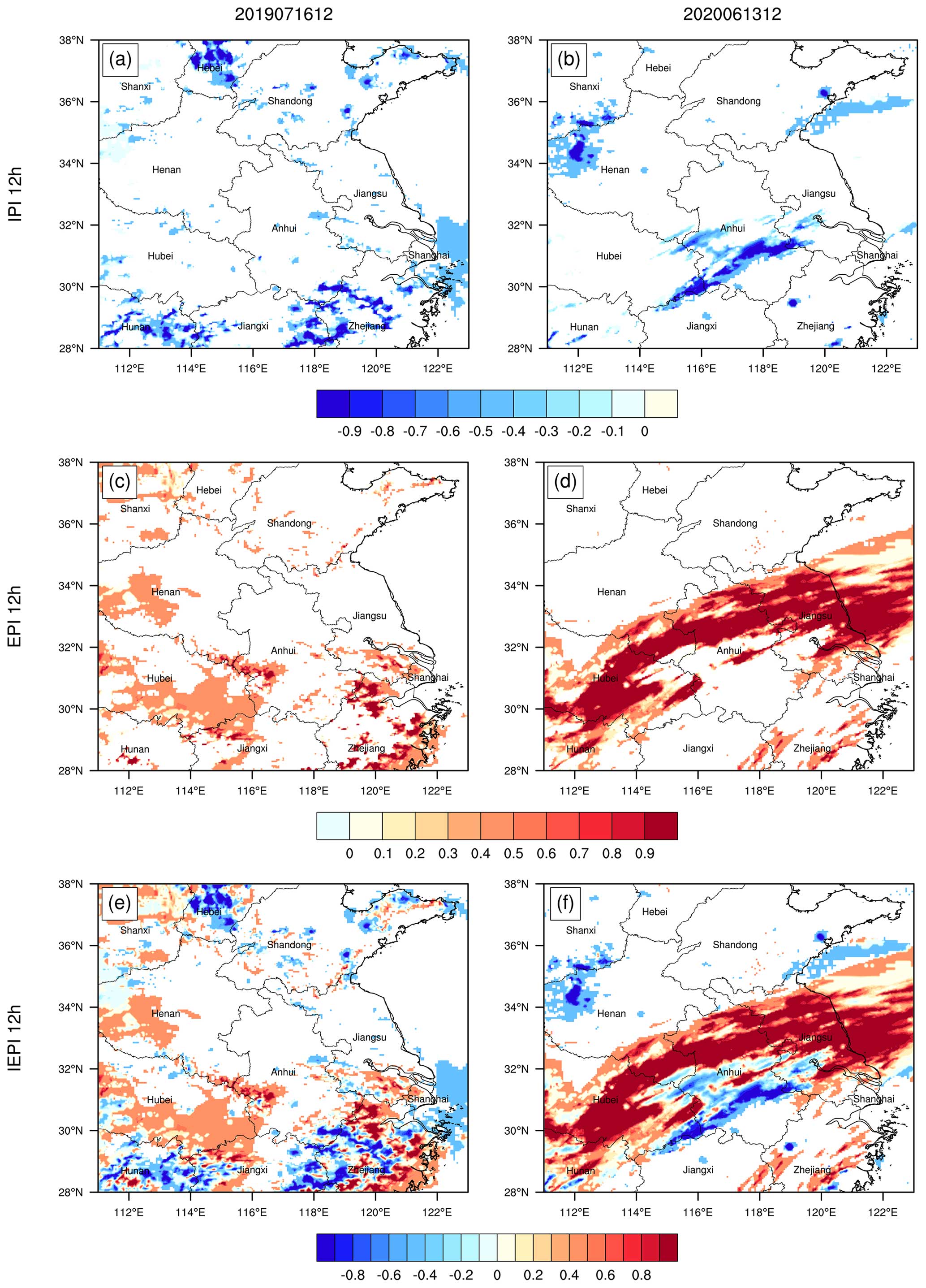
Figure 10 Distributions of IPI of 12 h accumulated precipitation for (a) Case 1 from 00:00 to 12:00 UTC on 16 July 2019 and (b) Case 2 from 00:00 to 12:00 UTC on 13 June 2020, EPI for (c) Case 1 and (d) Case 2, and IEPI for (e) Case 1 and (f) Case 2.

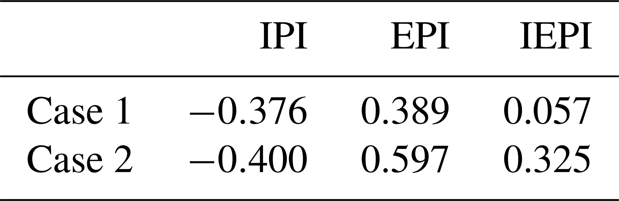
Figure 10 shows the IPI, EPI, and IEPI distributions of 12 h accumulated precipitation. In terms of the IPI, for Case 1, the large-value IPI areas are located at the intersection of Anhui, Zhejiang, and Jiangxi in the Hunan–Jiangxi region, as well as in the southern part of Hebei. For Case 2, the large-value IPI areas are situated along the Yangtze River in Anhui and Jiangxi, as well as at the intersection of Henan and Shanxi. The IPIs for Case 1 and Case 2 are −0.376 and −0.400, respectively, indicating that Case 2 shows a slightly higher level of insufficient forecasts (Table 10). In terms of the EPI, for Case 1, the large-value EPI areas are in Zhejiang and Jiangxi. In contrast, for Case 2, the large-value EPI areas are located in most of Hunan, Hubei, Anhui and Jiangsu, exhibiting a wide southwest–northeast orientation with a large area and degree. The EPI for Case 2 is larger than that for Case 1. The IEPI is a comprehensive reflection of under- and over-precipitation, and its value reflects the degree of insufficient and excessive precipitation forecasts. From the distributions of insufficient and excessive precipitation forecasts in Case 1, it is evident that the insufficient and excessive forecasts are roughly equivalent, with an IEPI of 0.057. However, for Case 2, the distribution of the excessive forecasts is obviously larger than that of the insufficient forecasts, with an IEPI of 0.325. This result indicates that Case 2 has poorer forecasting performance, with larger excessive forecasts being an important factor.

Table 10 Accuracy indices of insufficient precipitation forecast (IPI), excessive precipitation forecast (EPI), and insufficient and excessive precipitation forecast (IEPI) of 12 h accumulated precipitation for two precipitation processes.

Consequently, analyzing the locations of insufficient and excessive precipitation forecasts from the figures in conjunction with the characteristics of the forecasting process can provide useful insights for improving forecasts.

4.2 Comparison experiment of extreme-rainfall events

4.2.1 Introduction of the “July 2021” extreme-rainstorm event in Henan, China

From 17 to 23 July 2021, a rare extreme-rainstorm event occurred in Henan province, China. The extremely heavy rainstorm started in the southeastern region of Henan province on the morning of 17 July, then extended to the northern region, and ended on the morning of 23 July, lasting more than 6 d. The rainstorm occurred against the background of a typhoon, Huang–Huai vortex, shear line, and convergence line and was caused by the coupling of the low-level jet and boundary layer jet combined with the uplift of terrain (Wang et al., 2022; Su et al., 2021; Shi et al., 2021).

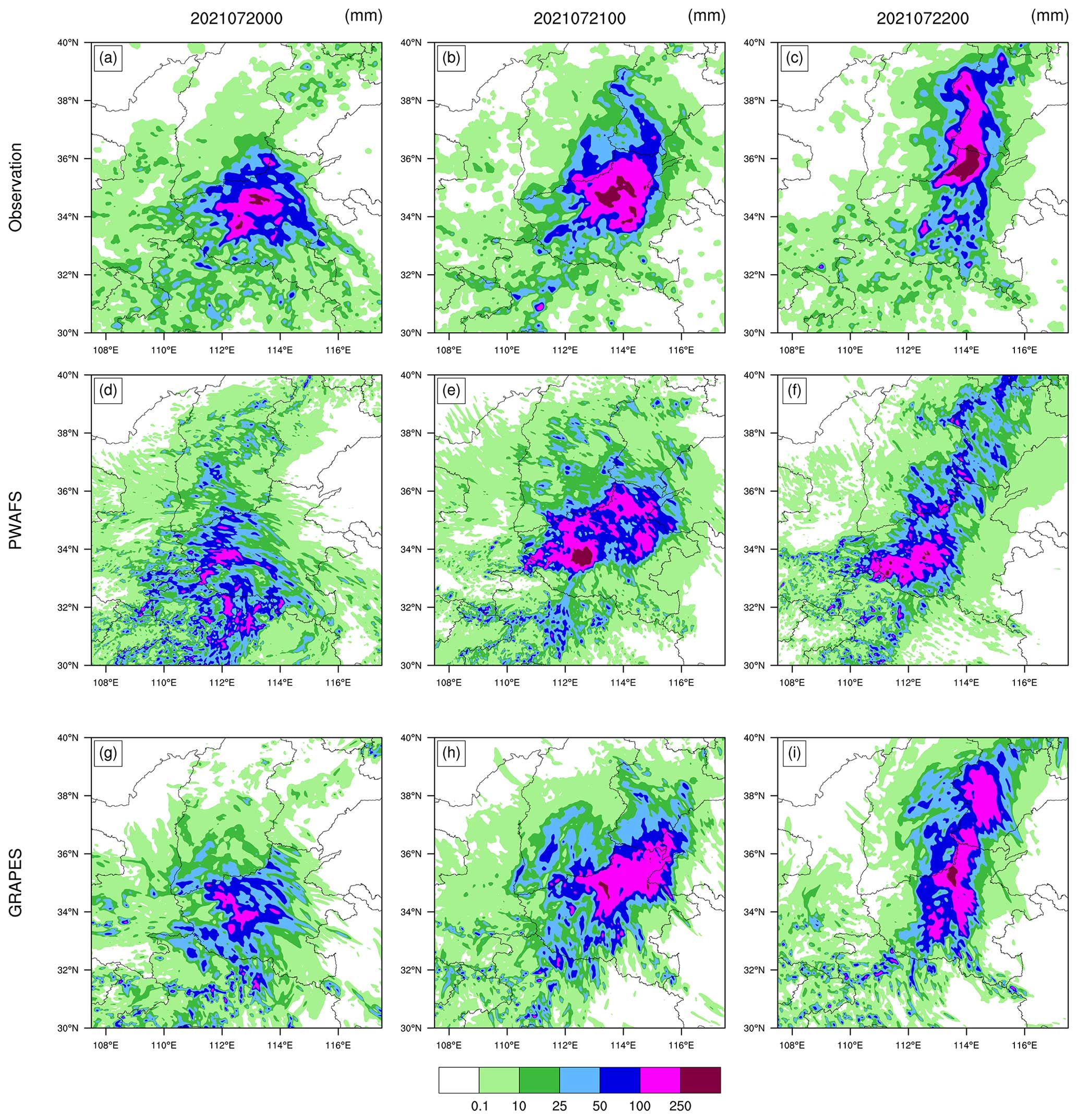
Figure 11 Distribution of observed and forecasted 24 h accumulated precipitation. (a) Observation, (d) PWAFS, and (g) GRAPES from 00:00 UTC on 19 July to 00:00 UTC on 20 July 2021. (b) Observation, (e) PWAFS, and (h) GRAPES from 00:00 UTC on 20 July to 00:00 UTC on 21 July 2021. (c) Observation, (f) PWAFS, and (i) GRAPES from 00:00 UTC on 21 July to 00:00 UTC on 22 July 2021.

The period from 00:00 UTC on 18 July to 00:00 UTC on 22 July 2021 is the concentrated period of heavy precipitation. To facilitate the study, the heavy-rainstorm process is divided into three periods: (1) 00:00 UTC on 19 July–00:00 UTC on 20 July 2021, (2) 00:00 UTC on 20 July–00:00 UTC on 21 July 2021, and (3) 00:00 UTC on 21 July–00:00 UTC on 22 July 2021 (Fig. 11a–c).

4.2.2 Data and methods

The observed precipitation data are provided by the CMPAS, with a spatial resolution of 0.05° × 0.05°, similar to the case in Sect. 4.1. The forecast data come from two models. One is the PWAFS model, which has a horizontal resolution of 3 km, similar to the case in Sect. 4.1. The other is the Global/Regional Assimilation and PrEdiction System (GRAPES) model independently developed by the China Meteorological Administration, which has a horizontal resolution of 3 km.

1. Determine the verification domain and verification points. The verification domain covers the region of 30–40° N, 107.5–117.5° E. The verification points are defined based on the grid points of the observed precipitation data; their spatial resolution is 0.05° × 0.05°, and the total number of verification grid points is 40 401 (201×201).

2. Prepare the observed and forecasted precipitation data and interpolate the forecasted precipitation data onto the observed grid points. The 24 h cumulative precipitation observation data of the three periods were obtained from the 24 h precipitation data of the CMPAS. The forecast precipitation data in the three periods are the cumulative precipitation with a forecast time of 12 to 36 h (Fig. 11d–i). For the case described in Sect. 4.1, the nearest-neighbor method is used to match the forecast data to the grid points of the observed precipitation.

3. Analyze the relationship between the forecasted precipitation and observed precipitation. PAS, TS, and FSS were compared for the extreme-rainstorm event in Henan, China.

As mentioned earlier, the FSS belongs to the neighborhood category of spatial verification methods and is an advanced evaluation method that has been widely used in recent years. It can still yield valuable scores when the model prediction intensity is spatially biased and can also represent the scale information of forecasting skills. Therefore, in this case, the FSS scoring method was added for comparative experiments. For FSS verification, 15, 25, 45, 75, and 120 km are used as the neighborhood distances.

The brief steps of FSS calculation are as follows: (1) determine the domain scope. Set the neighborhood point to n, such that when n=3 (n is odd), the neighborhood range is 15 km × 15 km. (2) Calculate the spatial density in the observed binary observation fields (Eq. 10). (3) Calculate the spatial density in the binary forecast fields (Eq. 11). (4) Calculate FSS_(n) (Eq. 12). (Please refer to the article of Roberts and Lean (2008) for details.)

$$\begin{array}{}\text{(10)}& {\displaystyle }\begin{array}{rl}O\left(n\right)\left(i,j\right)& ={\displaystyle \frac{\mathrm{1}}{n^{\mathrm{2}}}}{\sum }_{k=\mathrm{1}}^n\\ & \cdot {\sum }_{i=\mathrm{1}}^n{I}_{\mathrm{o}}\left[i+k-\mathrm{1}-{\displaystyle \frac{n-\mathrm{1}}{\mathrm{2}}},j+l-\mathrm{1}-{\displaystyle \frac{n-\mathrm{1}}{\mathrm{2}}}\right]\end{array},\text{(11)}& {\displaystyle }\begin{array}{rl}M\left(n\right)\left(i,j\right)& ={\displaystyle \frac{\mathrm{1}}{n^{\mathrm{2}}}}{\sum }_{k=\mathrm{1}}^n\\ & \cdot {\sum }_{i=\mathrm{1}}^n{I}_{\mathrm{M}}\left[i+k-\mathrm{1}-{\displaystyle \frac{n-\mathrm{1}}{\mathrm{2}}},j+l-\mathrm{1}-{\displaystyle \frac{n-\mathrm{1}}{\mathrm{2}}}\right]\end{array},\text{(12)}& {\displaystyle }{\mathrm{\text{FSS}}}_{\left(n\right)}=\mathrm{1}-{\displaystyle \frac{\frac{\mathrm{1}}{N_x{N}_y}{\sum }_{i=\mathrm{1}}^{N_x}{\sum }_{j=\mathrm{1}}^{N_y}{\left[O_{\left(n\right)i,j}-M_{\left(n\right)i,j}\right]}^{\mathrm{2}}}{\frac{\mathrm{1}}{N_x{N}_y}\left[{\sum }_{i=\mathrm{1}}^{N_x}{\sum }_{j=\mathrm{1}}^{N_y}{O}_{\left(n\right)i,j}^{\mathrm{2}}+{\sum }_{i=\mathrm{1}}^{N_x}{\sum }_{j=\mathrm{1}}^{N_y}{M}_{\left(n\right)i,j}^{\mathrm{2}}\right]}},\end{array}$$

where i ranges from 1 to N_x, N_x is the number of columns in the domain,  j ranges from 1 to N_y, and N_y is the number of rows. I_o and I_M are binary fields. O_(n)(i, j) is the resultant field of observed fractions for a square of length n. M_(n)(i, j) is the resultant field of model forecast fractions obtained.

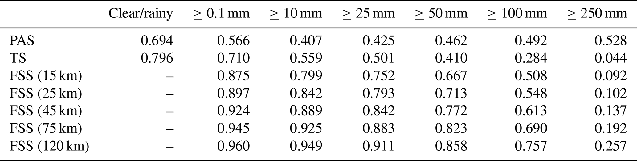
Table 11 PAS, TS, and FSS scores of PWAFS 24 h accumulated precipitation from 00:00 UTC on 19 July to 00:00 UTC on 20 July 2021.

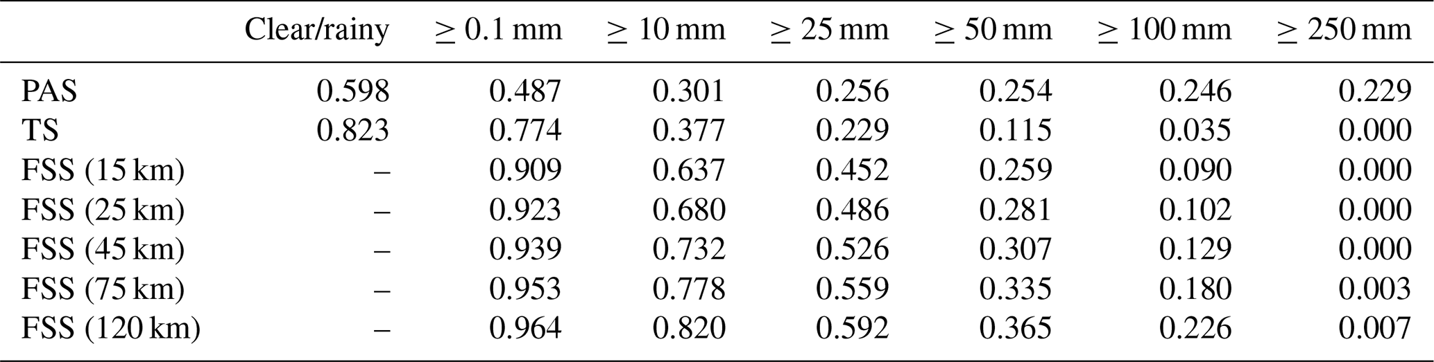
Table 12 PAS, TS, and FSS scores of PWAFS 24 h accumulated precipitation from 00:00 UTC on 20 July to 00:00 UTC on 21 July 2021.

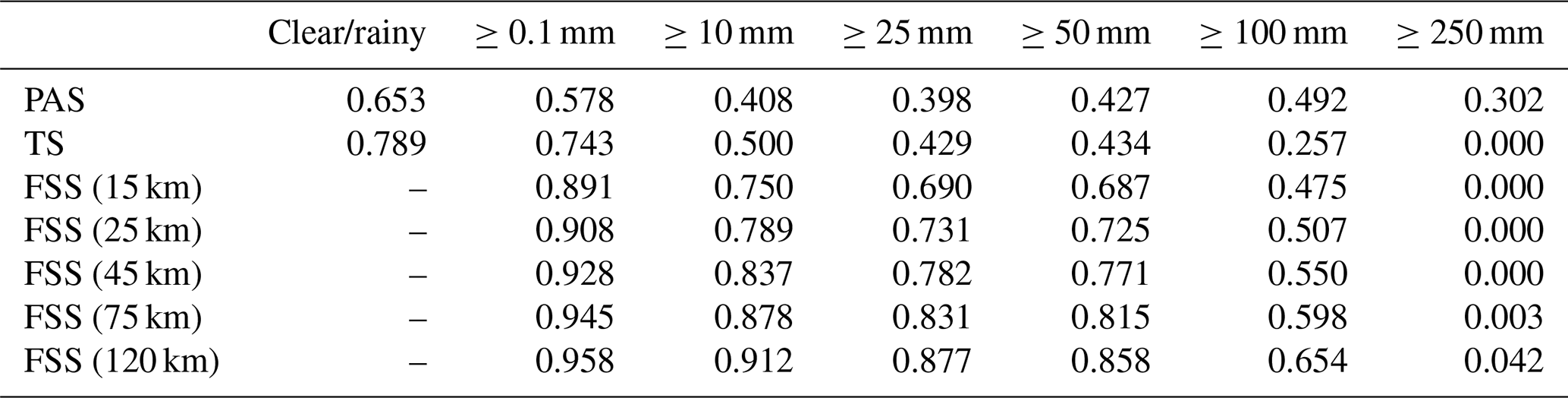
Table 13 PAS, TS, and FSS scores of PWAFS 24 h accumulated precipitation from 00:00 UTC on 21 July to 00:00 UTC on 22 July 2021.

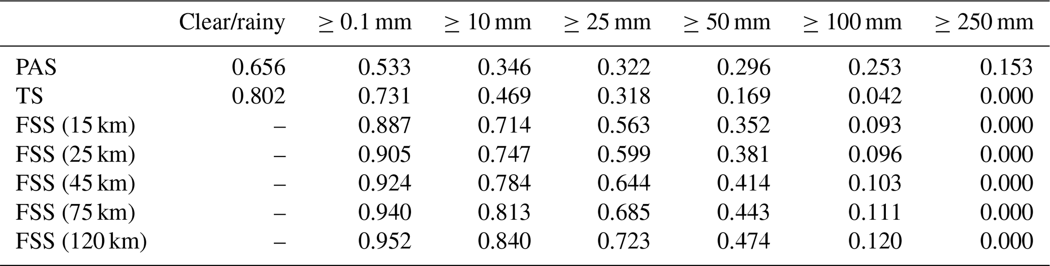
Table 14 PAS, TS, and FSS scores of GRAPES 24 h accumulated precipitation from 00:00 UTC on 19 July to 00:00 UTC on 20 July 2021.

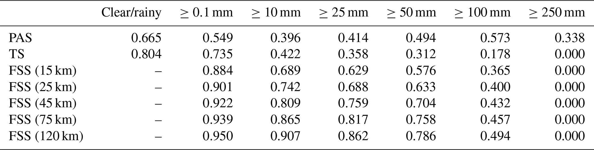
Table 15 PAS, TS, and FSS scores of GRAPES 24 h accumulated precipitation from 00:00 UTC on 20 July to 00:00 UTC on 21 July 2021.

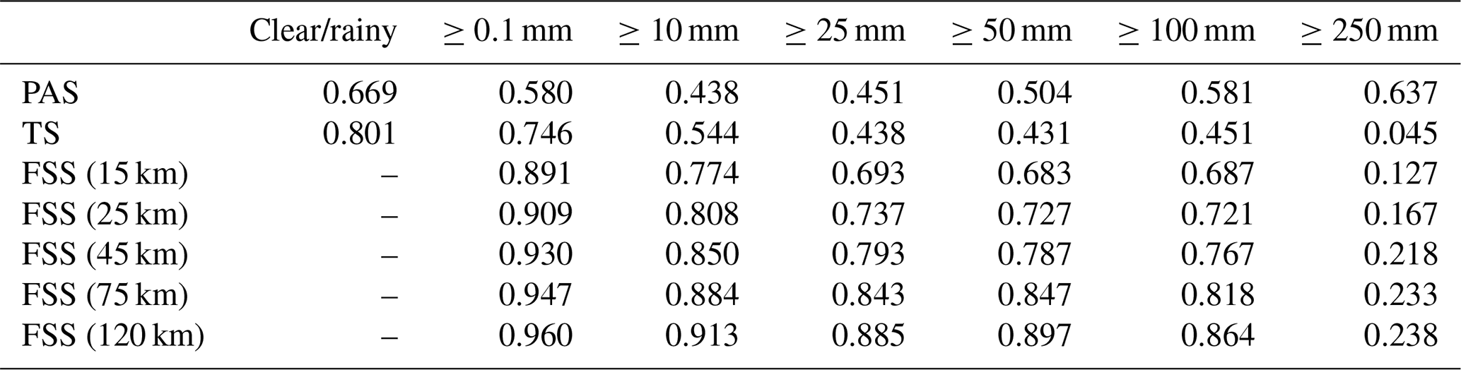
Table 16 PAS, TS, and FSS scores of GRAPES 24 h accumulated precipitation from 00:00 UTC on 21 July to 00:00 UTC on 22 July 2021.

4.2.3 Analysis of the comparative experiment results

1. Questionnaire survey of the effectiveness of model forecasting.

   In total, 52 questionnaires were completed by 32 researchers and 20 forecasters. The names of the PWAFS and GRAPES models used for comparison were omitted and replaced with Model 1 and Model 2, respectively.

   The survey results show that 52 people believe that the forecasting effect for periods A and C of Model 2 (GRAPES) is good, 19 people believe that the forecasting effect for period B of Model 1 (PWAFS) is good, and 33 people believe that the forecasting effect for period B of Model 2 (GRAPES) is good. A total of 52 people think that Model 2 (GRAPES) is good in general.

2. Indices analysis and comparison between the two models.

   The high-resolution regional models used for evaluation are (1) PWAFS 3 km and (2) GRAPES 3 km, and the modeled precipitation is the accumulated precipitation of 24 h in the forecast for 12–36 h. The evaluation results are as follows (Tables 11–16).

   The results show that in this process, the evaluation results of different methods on the forecast skill of the PWAFS and GRAPES models are basically consistent and in line with the subjective evaluation statistical results. However, PAS scores have obvious advantages in the evaluation of rainstorms and above, especially for extreme rainstorms. It can be seen from the six rating scales that the TS and FSS have almost no ability to evaluate precipitation above 250 mm, and the scores are generally at the unskilled end of 0 and no more than 0.2 (Chen et al., 2019). The PAS scores can also distinguish differences and provide different scores for situations where the forecasting effect is good.

   For example, when evaluating precipitation above 250 mm, the scores of TS for PWAFS in all three periods are 0.000, and the scores of GRAPES in the three periods are 0.000, 0.045, and 0.044. The scores of FSS (45 km) for the PWAFS in all three periods are 0.000, and the scores of GRAPES in the three periods are 0.000, 0.218, and 0.137, respectively. This indicates that the TS and FSS (45 km) have little ability to assess the heavy rainfall of this process.

   The PAS scores for PWAFS in the three periods are 0.229, 0.302, and 0.153, and those for GRAPES in the three periods are 0.338, 0.637, and 0.528, indicating that PAS has the ability to evaluate heavy rainstorms (above 250 mm) in this process. The evaluation results show that GRAPES is superior to PWAFS when predicting heavy rainfall.

   The evaluation capabilities of PAS, TS, and FSS for precipitation above 100 mm are further analyzed. The scores of TS for the PWAFS (GRAPES) are 0.035, 0.257, and 0.042 (0.178, 0.451, and 0.284) in the three periods, respectively. The scores of FSS (45 km) are 0.129, 0.550, and 0.103 (0.432, 0.767, and 0.613) for the PWAFS (GRAPES) in the three periods, respectively. The evaluation effect of FSS (45 km) is better than that of TS. The evaluation feature of FSS is to examine the predictability scale of the model to reflect its predictive ability; however, due to the subjectivity of selecting neighborhood scales, its score lacks comparability. While the PAS scores are 0.246, 0.492, and 0.253 (0.573, 0.581, and 0.492) for the PWAFS (GRAPES) in the three periods, it can be seen that the PAS also has a good ability to assess heavy rainstorms in this process.

   In small-magnitude precipitation (above light and moderate rain) verification, the FSS scores tend to approach 1 as the neighborhood distance expands, making it difficult to compare forecast differences between models. The PAS scores can also distinguish the differences in forecast effectiveness for small-magnitude precipitation.

In conclusion, different scoring methods were used to evaluate the skill of different models to predict extreme-precipitation events in July 2021 in Henan, China, and the evaluation characteristics of different scoring methods were indicated. The results show that the PAS scoring method has obvious advantages in the evaluation of extreme-precipitation events and can also reflect the differences in the small-magnitude precipitation forecasting effects of the models well compared to those of the TS and FSS methods.

5 Discussion and conclusion

By analyzing the advantages and disadvantages of the traditional TS, magnitude-improved TS, and neighborhood spatial verification methods, a new precipitation verification method, GCEM, was designed and constructed from the perspective of the proximity of the forecast to the observation. This method consists of the core indicator of the PAS, as well as multiple indicators such as IPI, EPI, IEPI, and PASC.

The PAS index consists of sine and e exponential functions. Additionally, considering the characteristics of large fluctuations in the function curves when observed precipitation is less than 10 mm, the formula has been smoothed for optimization. The PAS method adopts the principle of “classification before verification, no classification during verification”, which can serve as an alternative to skill scores such as the TS and ETS for verifying quantitative precipitation forecasts. This method is characterized by objective and transparent rules and easy generalization. Moreover, this approach possesses attributes of an ideal precipitation scoring method, such as fairness, boundedness, and moderate symmetry. Therefore, it can be used to calculate the accuracy of numerical models or quantitative precipitation forecasts, as well as evaluate the comprehensive forecasting capabilities of various refined quantitative precipitation forecast products. The GCEM can also evaluate the performance of numerical forecasts on clear/rain forecasts, as well as insufficient precipitation forecasts, excessive precipitation forecasts, and precipitation forecast biases. In addition to the overall score, two-dimensional score distribution maps can be generated for each index in the GCEM system. These maps offer a comprehensive reflection of the precipitation forecasting performance of the numerical models and serve as a reference for improving model forecasts.

This new verification method is validated based on the forecast scoring results for general precipitation and precipitation at the level of torrential rain and above, and the verification results align with expectations. Comparative experiments are also conducted on two typical processes using the new verification method. For Case 1, the subjective judgment is relatively good, but the TS is lower. Conversely, for Case 2, the subjective judgment is poorer, yet the TS is higher. Verification using the PAS reveals that forecasts with better subjective judgment receive higher scores, and forecasts with poorer subjective judgment receive lower scores. Therefore, PAS aligns with public expectations.

The PAS, TS, and FSS methods were used to compare and verify the July 2021 extreme-precipitation event in Henan, China, to reflect the evaluation characteristics of different scoring methods. The results show that the PAS scoring method can not only reflect the difference in the small-magnitude precipitation forecast effect of models but also has obvious advantages in the evaluation of extreme-precipitation events.

In addition, the National Meteorological Centre of China conducted a long-term series of large-scale sample testing on this method in 2023. Based on the ECMWF model's 24 and 48 h precipitation forecasts from March 2022 to February 2023, the assessment results show that compared to the TS, the PAS is less affected by the randomness of the sample, and the relative size relationship of different time forecast scores is more stable.

From the construction of the GCEM to ideal experiments and case analysis, it is evident that this evaluation system, especially the PAS method, is a suitable method for quantitative precipitation evaluation. However, the PAS still has subjective flaws, such as the determination of coefficients in the PAS expression (0.6 in Eqs. 6 and 7) when the observed or forecasted precipitation is 0 mm. Once these coefficients are determined, they apply to all precipitation scoring, thus becoming an objective component in practice.