The community-centered freshwater biogeochemistry model unified RIVE v1.0: a unified version for water column

Research on mechanisms of organic matter degradation, bacterial activities, phytoplankton dynamics, and other processes has led to the development of numerous sophisticated water quality models. The earliest model, dating back to 1925, was based on first-order kinetics for organic matter degradation. The community-centered freshwater biogeochemistry model RIVE was initially developed in 1994 and has subsequently been integrated into several software programs such as Seneque-Riverstrahler, pyNuts-Riverstrahler, ProSe/ProSe-PA, and Barman. After 30 years of research, the use of different programming languages including QBasic, Visual Basic, Fortran, ANSI C, and Python, as well as parallel evolution and the addition of new formalisms, raises questions about their comparability.

This paper presents a unified version of the RIVE model for the water column, including formalisms for bacterial communities (heterotrophic and nitrifying), primary producers, zooplankton, nutrients, inorganic carbon, and dissolved oxygen cycles. The unified RIVE model is open-source and implemented in Python 3 to create pyRIVE 1.0 and in ANSI C to create C-RIVE 0.32. The organic matter degradation module is validated by simulating batch experiments. The comparability of the pyRIVE 1.0 and C-RIVE 0.32 software is verified by modeling a river stretch case study. The case study considers the full biogeochemical cycles (microorganisms, nutrients, carbon, and oxygen) in the water column, as well as the effects of light and water temperature. The results show that the simulated concentrations of all state variables, including microorganisms and chemical species, are very similar for pyRIVE 1.0 and C-RIVE 0.32. This open-source project highly encourages contributions from the freshwater biogeochemistry community to further advance the project and achieve common objectives.

1 Introduction

Modeling the water quality of a freshwater system (river, lake, or reservoir) is critical to understanding and managing its functioning. The functioning of a freshwater system is the result of complex interrelated biogeochemical processes. The first water quality model developed by Streeter and Phelps (1925) describes the degradation of organic matter (OM) in a river. The organic matter, measured globally by biochemical oxygen demand in 5 d (BOD5), is considered to be degraded according to first-order kinetics. Although dating back more than a century (the study was completed in 1915, but publication was delayed to 1925 due to World War I; Hellweger, 2015), this model is still widely used to represent the dynamics of organic matter in water quality modeling (Hellweger, 2015).

While the role of microorganisms in the degradation of organic matter has been acknowledged since the end of the 19th century, there is an important limitation of this type of representation. The microbiological nature of the organic matter degradation process and the bacterial population dynamics intrinsically involved are completely obscured. They are implicitly taken into account only through a biodegradability constant of organic matter and its dependence on temperature. Microbial biogeochemical work in the 1980s–1990s led to the elucidation of the detailed mechanisms of the organic matter degradation process and the associated heterotrophic bacterial activities (Fuhrman and Azam, 1982; Azam et al., 1983; Somville and Billen, 1983; Servais et al., 1985; Rego et al., 1985; Fontigny et al., 1987; Servais et al., 1987; Billen et al., 1988; Servais et al., 1989; Billen et al., 1990; Garnier et al., 1992a, b). This new corpus of knowledge led to the development and the formulation of the biogeochemical model RIVE (Billen et al., 1994; Garnier and Billen, 1994). It is capable of simulating the degradation of OM in freshwater systems and the associated oxygen consumption by bacterial activities, which is more realistic than the model of Streeter and Phelps (1925). In the RIVE model, the HSB model (Billen and Servais, 1989; Billen, 1991) is used to represent the degradation of organic matter and heterotrophic bacterial activities. This model simulates the exoenzymatic hydrolysis of particulate and dissolved organic matter (split into biodegradable and refractory pools), including high-weight polymers, into small monomeric substrates. These substrates are subsequently assimilated by bacteria for their growth and respiration.

Apart from the degradation of organic matter, the AQUAPHY model (Lancelot et al., 1991) is used to simulate the dynamics of phytoplankton in the RIVE model (Billen et al., 1994). The model explicitly simulates photosynthesis of phytoplankton, growth, mortality, and respiration processes. In addition to water temperature, the photosynthesis depends on the light intensity, while growth is controlled by nutrient availability and small organic metabolites. The small organic metabolites are formed either directly by photosynthesis or by catabolysis of reserve products. This conceptualization allows for the growth of phytoplankton during dark periods. In addition, the model also introduces a limiting factor of nutrients in the growth of phytoplankton and considers the cycling of nutrients during the life cycle of phytoplankton.

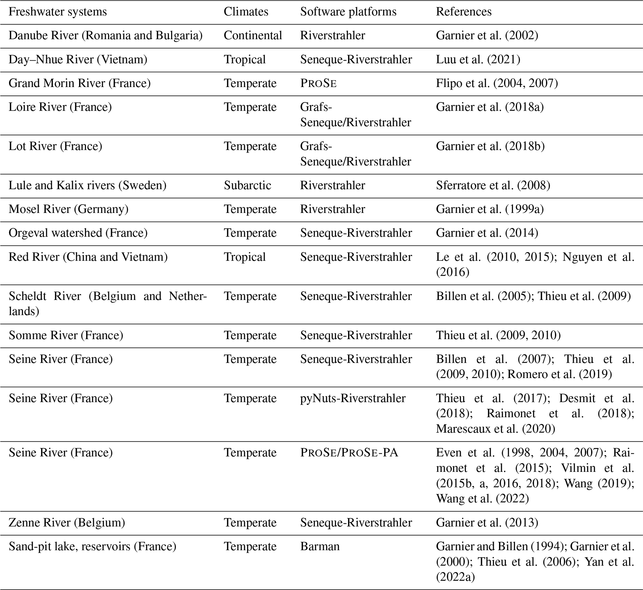
Since its initial development by Billen et al. (1994), the RIVE model has co-existed within several software packages (Table A1) developed for different aquatic compartments and supported by the PIREN-Seine program (https://www.piren-seine.fr/, last access: 20 December 2023). The RIVE model was firstly applied in river systems using the Riverstrahler drainage network approach (Billen et al., 1994; Garnier et al., 1995). It was initially coded in QBasic and later on piloted by a GIS graphical interface, Seneque-Riverstrahler (Visual Basic; Ruelland et al., 2007). And it is now fully integrated within the pyNuts-Riverstrahler (https://gitlab.in2p3.fr/rive/pynuts/, last access: 20 December 2023) Python framework (Thieu et al., 2017). It can model the biogeochemical functioning of hydrographic networks at scales ranging from local to continental. The RIVE model was also applied to lentic freshwater systems like regulated reservoirs (Barman software, Garnier et al., 2000; Thieu et al., 2006; Yan et al., 2022a – Table A1) or to simulate hydro-biodynamic functioning of highly human-impacted river systems (ProSe software – Even et al., 1998, 2004, 2007; Flipo et al., 2004; Vilmin et al., 2015b; ProSe-PA software – Wang et al., 2019, 2023a, https://gitlab.com/prose-pa/prose-pa last access: 20 December 2023; developed in ANSI C coupled with a self-developed lex and yacc parser; Table A1). The RIVE model is also coupled with the Soil & Water Assessment Tool (SWAT) to simulate the water quality of the Vienne basin, France (Manteaux et al., 2023), and incorporated into the QUAL-NET model (Minaudo et al., 2018) to simulate river eutrophication in the drainage network of the middle Loire River corridor, France. Moreover, the RIVE model is implemented into the VEMALA V3 model to simulate phosphorus and nitrogen loading in Finnish watersheds (Korppoo et al., 2017).

Based on the above implementations, different versions of the RIVE model code have successfully simulated a large variety of freshwater systems (lake or reservoirs, river systems) across the world. The parameter values were determined through laboratory experiments or calibrated with observation data (Garnier et al., 1992a; Servais and Garnier, 1993; Garnier and Billen, 1994; Billen et al., 1994; Garnier et al., 1995). These applications (Table A1) were carried out for different networks and scales as well as various degrees of anthropogenic impacts in a wide climatic gradient using either Riverstrahler (possibly with its Seneque or pyNuts environments) or ProSe/ProSe-PA, such as the Seine River (France) (Billen et al., 1994; Garnier et al., 1995; Even et al., 1998, 2004, 2007; Billen et al., 2007; Servais et al., 2007; Thieu et al., 2009, 2010; Vilmin et al., 2015b, a; Aissa-Grouz et al., 2016; Vilmin et al., 2016; Desmit et al., 2018; Vilmin et al., 2018; Romero et al., 2019; Marescaux et al., 2020; Wang et al., 2022), the Danube River (Romania and Bulgaria) (Garnier et al., 2002), the Red River (China and Vietnam) (Le et al., 2010, 2015; Nguyen et al., 2016) and its distributary the Day–Nhue River (Luu et al., 2021), the Lule and Kalix rivers (Sweden) (Sferratore et al., 2008), the Scheldt river (Belgium and Netherlands) (Billen et al., 2005; Thieu et al., 2009), the Zenne River (Belgium) (Garnier et al., 2013), the Mosel River (Germany) (Garnier et al., 1999a), the Somme River (France) (Thieu et al., 2009, 2010), the Loire River (France) (Garnier et al., 2018a), the Lot River (France) (Garnier et al., 2018b), and the Orgeval watershed (France) (Flipo et al., 2004, 2007; Garnier et al., 2014). Moreover, the RIVE model has also been applied to stagnant systems (e.g., sand-pit lake – Lake Crétail, France, Garnier and Billen, 1994; reservoirs – Marne, Aube, Seine, France, Garnier et al., 2000; Yan et al., 2022a).

After 30 years of research, the parallel evolutions of these codes, the numerical adaptations inherent in programming languages (QBasic, Visual Basic, Fortran, Python, and ANSI C), and the addition of new formalisms raise the question of their comparability. The identification of a unified version of the RIVE model is then necessary. A project aiming at unifying these RIVE implementations was undertaken. The unified version brings together all recent developments, especially the ones achieved with Python and ANSI C programming languages. This action will strengthen the collaboration of the research teams involved in the development of the model. This paper presents a unified version of RIVE for the water column (called unified RIVE v1.0) with a presentation of the formalisms for the biogeochemical cycles. That integrates the bacterial communities (heterotrophic and nitrifying), primary producers, zooplankton, and fate of detritic organic matter either particulate or dissolved and as biodegradable and refractory, as well as the associated nutrients and dissolved oxygen cycles. The most recent developments in modeling inorganic forms of carbon are also presented. The unified RIVE v1.0 included in pyRIVE 1.0 (tested with Python 3 versions up to 3.10 release) and C-RIVE 0.32 is open-source and therefore available to the scientific community. A numerical experiment is then introduced to evaluate the comparability of the pyRIVE 1.0 and C-RIVE 0.32 through a systematic comparison of simulations produced under controlled conditions. We thus establish a reference framework to evaluate different implementations (programming languages, performance – comparability) of the unified RIVE v1.0 formulation that continues to evolve in several water quality models.

2 Model description

The unified RIVE v1.0 model simulates the cycling of carbon, nutrients, and oxygen within a freshwater system (river, lake, reservoir). Biogeochemical cycles are simulated with a community-centered or agent-based model. That means that the freshwater system functioning is explicitly modeled, taking into consideration the activities of microorganisms such as phytoplankton, zooplankton, heterotrophic bacteria, and nitrifying bacteria. Additionally, it accounts for physical processes like oxygen re-aeration and dilution. This modeling approach is developed in relation to water temperature, macronutrients, and organic matter, (particulate, dissolved, and biodegradable fractions). The organic matter degradation, nitrifying bacteria dynamics, primary producer dynamics, zooplankton dynamics, nutrients, and inorganic carbon cycling are described subsequently. A high number of model parameters are used to characterize the microorganisms' properties and most of them have been determined through field or laboratory experiments under controlled conditions. This paper presents a focus on the conceptualization of the unified RIVE v1.0 model in the water column exclusively. While the RIVE model does have applications for sediment dynamics and its interaction with the water column (Even et al., 2004; Thouvenot et al., 2007; Billen et al., 2015; Vilmin et al., 2015a, 2016; Yan et al., 2022b), relevant community-centered efforts need to be made in future work, which is not the focus of this study.

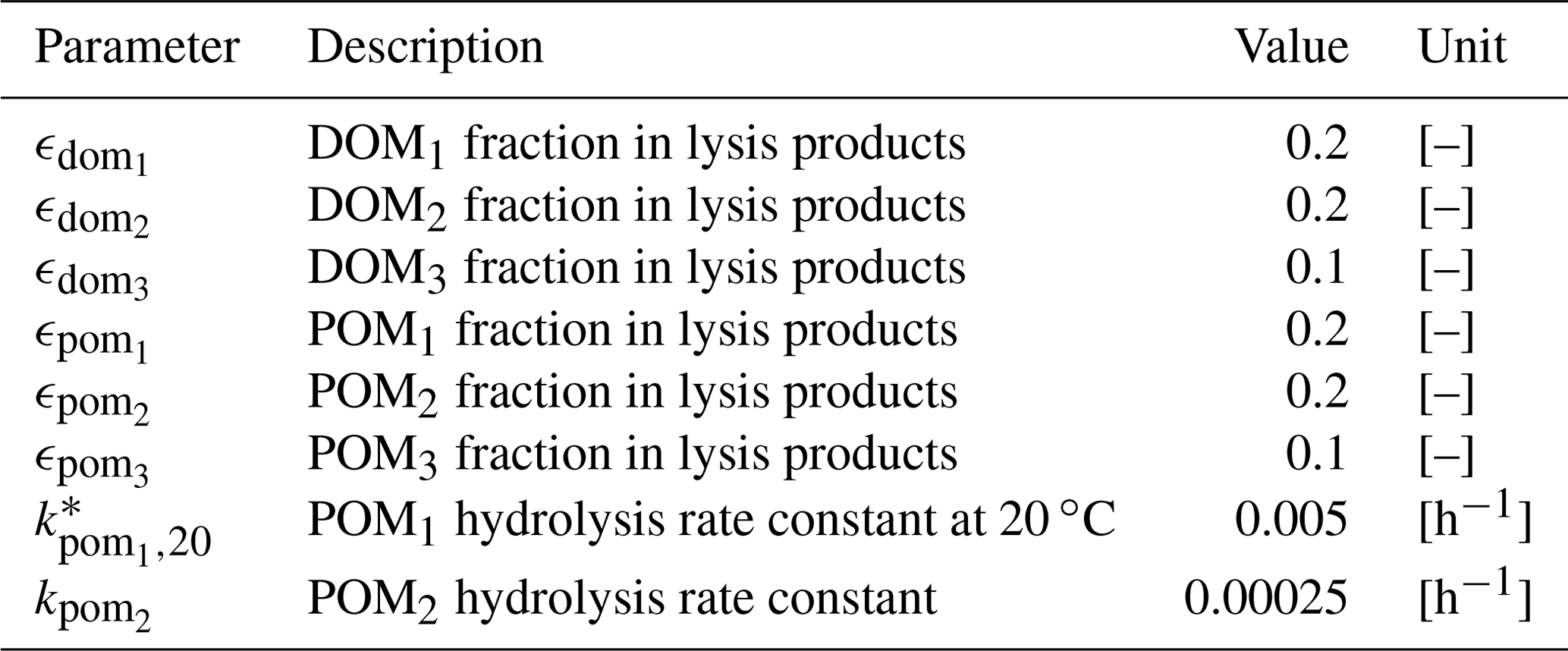
2.1 Organic matter degradation

The mechanisms of organic matter degradation by the activity of heterotrophic bacteria are represented using the HSB model (Billen and Servais, 1989; Billen, 1991). It contains three variables: H represents high-weight polymers (large molecules), which form the majority of dissolved and particulate organic matter but must be exoenzymatically hydrolyzed to be accessible to heterotrophic bacteria; S represents small monomeric substrates (SMSs), directly accessible to microbial uptake; and B represents heterotrophic bacteria that absorb the substrates for their growth and respiration (Fig. 1). In diagrams of this paper (for instance the HSB model, Fig. 1), the state variables are shown as circles and represent either concentrations or stocks entering and leaving the (biogeochemical) processes. The biogeochemical processes are represented by squares.

The high-weight polymer (total organic carbon) is conceptually divided for each phase (dissolved – HD; particulate – HP) into three pools. Each pool is characterized by a specific biodegradability: (1) rapidly biodegradable in 5 d (HD₁ and HP₁), (2) slowly biodegradable in 45 d (HD₂ and HP₂), and (3) refractory (HD₃ and HP₃).

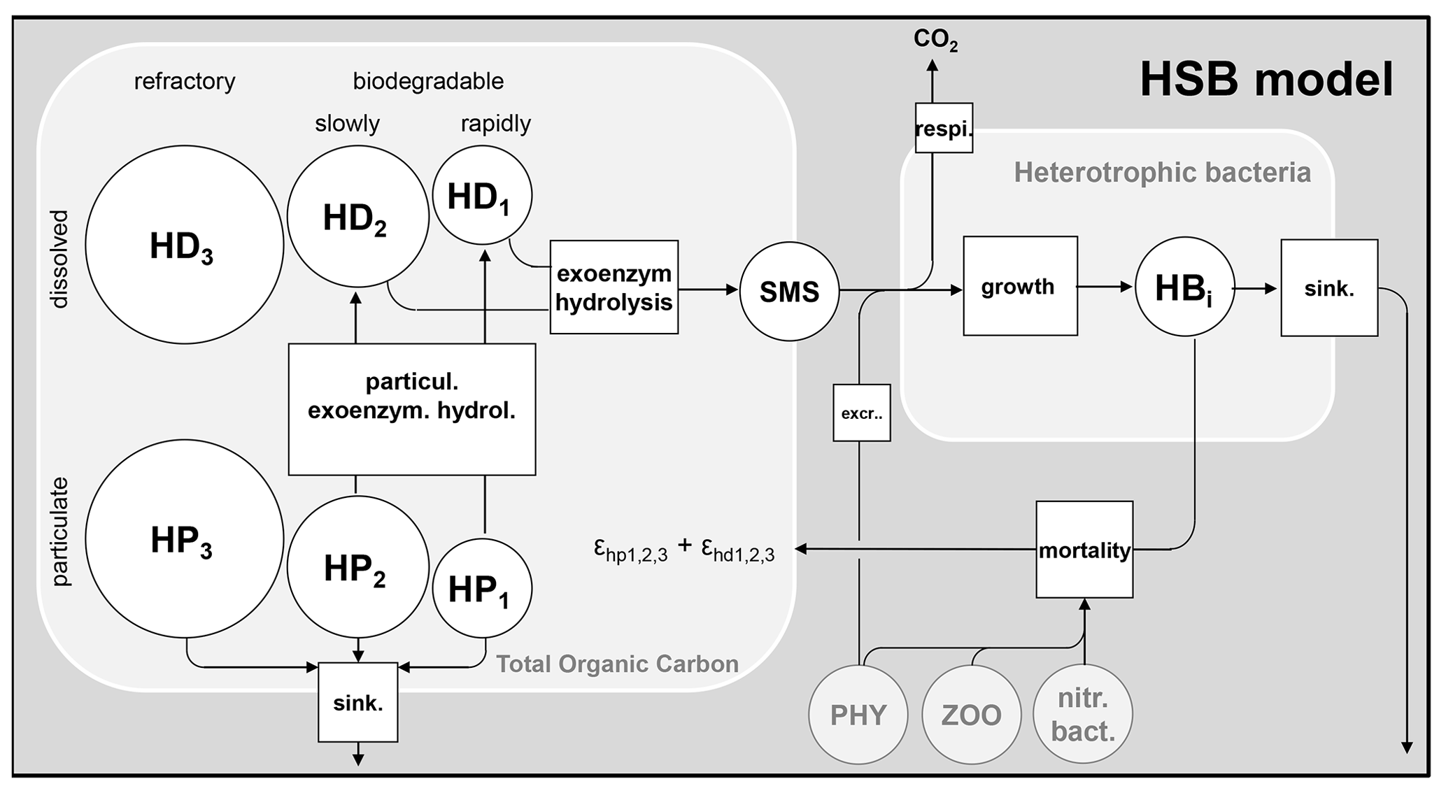
Figure 1 Flowchart of the HSB model. HD: dissolved high-weight polymer; HP: particulate high-weight polymer; SMS: small monomeric substrate; HB: heterotrophic bacteria; PHY: phytoplankton; ZOO: zooplankton; nitr. bact.: nitrifying bacteria; extr. excretion of phytoplankton; sink.: sinking. respi.: respiration; ${\mathit{ϵ}}_{\mathrm{hp}\mathrm{1},\mathrm{2},\mathrm{3}}$ and ${\mathit{ϵ}}_{\mathrm{hd}\mathrm{1},\mathrm{2},\mathrm{3}}$: proportion to convert dead biomass to HP and HD.

2.1.1 Heterotrophic bacteria dynamics

The dynamic of heterotrophic bacteria is explicitly simulated, including growth, mortality, and respiration. The growth of heterotrophic bacteria depends on water temperature and the availability of small monomeric substrate (SMS). The dependence is represented by the Monod equation (Monod, 1949). A maximal substrate uptake rate at 20 ^∘C (b_max20,hb) and a bacterial growth yield (Y_hb) are used to calculate the growth rate of heterotrophic bacteria (${\mathit{\mu }}_{{\mathrm{hb}}_i}$) (Eq. 3). The fraction of uptake not used for growth (1−Y_hb) is respired.

$$\begin{array}{}\text{(1)}& {\displaystyle }{b}_{{\mathrm{hb}}_i}=b_{\max \mathrm{20},{\mathrm{hb}}_i}f(T{)}_{{\mathrm{hb}}_i}{\displaystyle \frac{\left[\mathrm{SMS}\right]}{\left[\mathrm{SMS}\right]+K_{\mathrm{sms},{\mathrm{hb}}_i}}}\text{(2)}& {\displaystyle }f(T{)}_{{\mathrm{hb}}_i}={\displaystyle \frac{e^{-\frac{{\left(T-T_{\mathrm{opt},{\mathrm{hb}}_i}\right)}^{\mathrm{2}}}{{\mathit{\sigma }}_{{\mathrm{hb}}_i}^{\mathrm{2}}}}}{e^{-\frac{{\left(\mathrm{20}-T_{\mathrm{opt},{\mathrm{hb}}_i}\right)}^{\mathrm{2}}}{{\mathit{\sigma }}_{{\mathrm{hb}}_i}^{\mathrm{2}}}}}}\text{(3)}& {\displaystyle }{\mathit{\mu }}_{{\mathrm{hb}}_i}=Y_{{\mathrm{hb}}_i}{b}_{{\mathrm{hb}}_i}\end{array}$$

Here, $b_{{\mathrm{hb}}_i}$ is the effective substrate uptake rate of the ith species of heterotrophic bacteria [h⁻¹], $b_{\max \mathrm{20},{\mathrm{hb}}_i}$ is the maximal substrate uptake rate of the ith species of heterotrophic bacteria at 20 ^∘C [h⁻¹], [SMS] is the small monomeric substrate concentration [mgC L⁻¹], $K_{\mathrm{sms},{\mathrm{hb}}_i}$ is the half-saturation constant for small monomeric substrate of the ith species of heterotrophic bacteria [mgC L⁻¹], $f(T{)}_{{\mathrm{hb}}_i}$ is the water temperature weight of the ith species of heterotrophic bacteria at T ^∘C [–], $T_{\mathrm{opt},{\mathrm{hb}}_i}$ is the optimal temperature of the ith species of heterotrophic bacteria for its growth [^∘C], ${\mathit{\sigma }}_{{\mathrm{hb}}_i}$ is the range of temperature for the ith species of heterotrophic bacteria [^∘C], $Y_{{\mathrm{hb}}_i}$ is the bacterial growth yield of the ith species of heterotrophic bacteria [–], and ${\mathit{\mu }}_{{\mathrm{hb}}_i}$ is the effective growth rate of the ith species of heterotrophic bacteria [h⁻¹]

A sinking velocity (vs_hb) is associated with each particulate species to represent particulate sinking by gravity. The mortality of heterotrophic bacteria is simulated by first-order kinetics (Eq. 4). The dead biomass of living species is converted into varying types of organic matter content, including both dissolved and particulate forms, based on specified proportions (ϵ_hd and ϵ_hp, Fig. 1).

$$\begin{array}{}\text{(4)}& \begin{array}{rl}& {\displaystyle \frac{\mathrm{d}\left[{\mathrm{HB}}_i\right]}{\mathrm{d}t}}=({\mathit{\mu }}_{{\mathrm{hb}}_i}-k_{\mathrm{d}\mathrm{20},{\mathrm{hb}}_i}f(T{)}_{{\mathrm{hb}}_i}-k_{\mathrm{sink},{\mathrm{hb}}_i}\left)\right[{\mathrm{HB}}_i]\\ & k_{\mathrm{sink},{\mathrm{hb}}_i}={\displaystyle \frac{{\mathrm{vs}}_{{\mathrm{hb}}_i}}{\mathrm{depth}}}\end{array}\end{array}$$

Here, ${\mathit{\mu }}_{{\mathrm{hb}}_i}$ is the effective growth rate of the ith species of heterotrophic bacteria [h⁻¹], $k_{\mathrm{d}\mathrm{20},{\mathrm{hb}}_i}$ is the mortality rate of the ith species of heterotrophic bacteria at 20 ^∘C [h⁻¹], $k_{\mathrm{sink},{\mathrm{hb}}_i}$ is the sinking rate of the ith species of heterotrophic bacteria [h⁻¹], [HB_i] is the biomass concentration of the ith species of heterotrophic bacteria [mgC L⁻¹], $f(T{)}_{{\mathrm{hb}}_i}$ is the water temperature weight at T ^∘C defined by Eq. (2) [–], ${\mathrm{vs}}_{{\mathrm{hb}}_i}$ is the sinking velocity of the ith species of heterotrophic bacteria [m h⁻¹], and “depth” represents the water depth [m].

2.1.2 Hydrolysis of high-weight polymer

The particulate biodegradable high-weight polymer (HP₁ and HP₂) is firstly hydrolyzed to the dissolved biodegradable high-weight polymer (HD₁ and HD₂). The dissolved biodegradable high-weight polymer is then hydrolyzed exoenzymatically to small monomeric substrate (Fig. 1). The hydrolysis of HP is represented by first-order kinetics (Eq. 5), while a Michaelis–Menten function (Michaelis and Menten, 1913) is used to express the exoenzymatic hydrolysis of HD (Eq. 6).

$$\begin{array}{}\text{(5)}& \begin{array}{rl}{\displaystyle \frac{\mathrm{d}\left[{\mathrm{HP}}_i\right]}{\mathrm{d}t}}& =-k_{{\mathrm{hp}}_i}\times \left[{\mathrm{HP}}_i\right]+\left(\sum _j{k}_{\mathrm{d}\mathrm{20},j}f\left(T{)}_j\right[\mathrm{LS}{]}_j\right)\\ & {\mathit{ϵ}}_{{\mathrm{hp}}_i}-k_{\mathrm{sink},{\mathrm{hp}}_i}\left[{\mathrm{HP}}_i\right]\end{array}\end{array}$$

Here, [HP_i] is the concentration of particulate high-weight polymer $i\in \mathit{\{}\mathrm{1},\mathrm{2}\mathit{\}}$ [mgC L⁻¹], $k_{{\mathrm{hp}}_i}$ is the hydrolysis rate of HP_i ($i\in \mathit{\{}\mathrm{1},\mathrm{2}\mathit{\}}$) [h⁻¹], f(T)_j is the water temperature weight of the jth living species at T ^∘C defined as in Eq. 2 [–], k_d20,j is the mortality rate of the jth living species (such as phytoplankton, zooplankton, bacteria) at 20 ^∘C [h⁻¹], [LS]_j is the concentration of the jth living species [mgC L⁻¹], ${\mathit{ϵ}}_{{\mathrm{hp}}_i}$ is the proportion to convert the dead biomass to HP_i ($i\in \mathit{\{}\mathrm{1},\mathrm{2}\mathit{\}}$) [–], and $k_{\mathrm{sink},{\mathrm{hp}}_i}$ is the sinking rate for HP_i ($i\in \mathit{\{}\mathrm{1},\mathrm{2}\mathit{\}}$) [h⁻¹].

$$\begin{array}{}\text{(6)}& \begin{array}{rl}{\displaystyle \frac{\mathrm{d}\left[{\mathrm{HD}}_i\right]}{\mathrm{d}t}}& =-\sum _k\left(e_{\max \mathrm{20},{\mathrm{hd}}_i,h{b}_k}f(T{)}_{{\mathrm{hb}}_k}{\displaystyle \frac{\left[{\mathrm{HD}}_i\right]}{\left[{\mathrm{HD}}_i\right]+K_{{\mathrm{hd}}_i,{\mathrm{hb}}_k}}}\right.\\ & \left.\left[{\mathrm{HB}}_k\right]\right)+k_{{\mathrm{hp}}_i}\times \left[{\mathrm{HP}}_i\right]\\ & +\left(\sum _j{k}_{\mathrm{d}\mathrm{20},j}f\left(T{)}_j\right[\mathrm{LS}{]}_j\right){\mathit{ϵ}}_{{\mathrm{hd}}_i}\end{array}\end{array}$$

Here, [HD_i] is the concentration of dissolved high-weight polymer ($i\in \mathit{\{}\mathrm{1},\mathrm{2}\mathit{\}}$) [mgC L⁻¹], $e_{\max \mathrm{20},{\mathrm{hd}}_i,{\mathrm{hb}}_k}$ is the maximum hydrolysis rate of HD_i at 20 ^∘C related to HB_k and $i\in \mathit{\{}\mathrm{1},\mathrm{2}\mathit{\}}$ [h⁻¹], $f(T{)}_{{\mathrm{hb}}_k}$ is the water temperature weight of the kth species of heterotrophic bacteria at T ^∘C (Eq. 2) [–], $K_{{\mathrm{hd}}_i,{\mathrm{hb}}_k}$ is the half-saturation constant for HD_i related to HB_k and $i\in \mathit{\{}\mathrm{1},\mathrm{2}\mathit{\}}$ [mgC L⁻¹], [HB_k] is the concentration of the kth species of heterotrophic bacteria [mgC L⁻¹], k_d20,j is the mortality rate of the jth living species (such as phytoplankton, zooplankton, bacteria) at 20 ^∘C [h⁻¹], f(T)_j is the water temperature weight of the jth living species at T ^∘C defined as in Eq. (2) [–], [LS]_j is the concentration of the jth living species [mgC L⁻¹], and ${\mathit{ϵ}}_{{\mathrm{hd}}_i}$ is the proportion to convert the dead biomass to HD_i and $i\in \mathit{\{}\mathrm{1},\mathrm{2}\mathit{\}}$ [–].

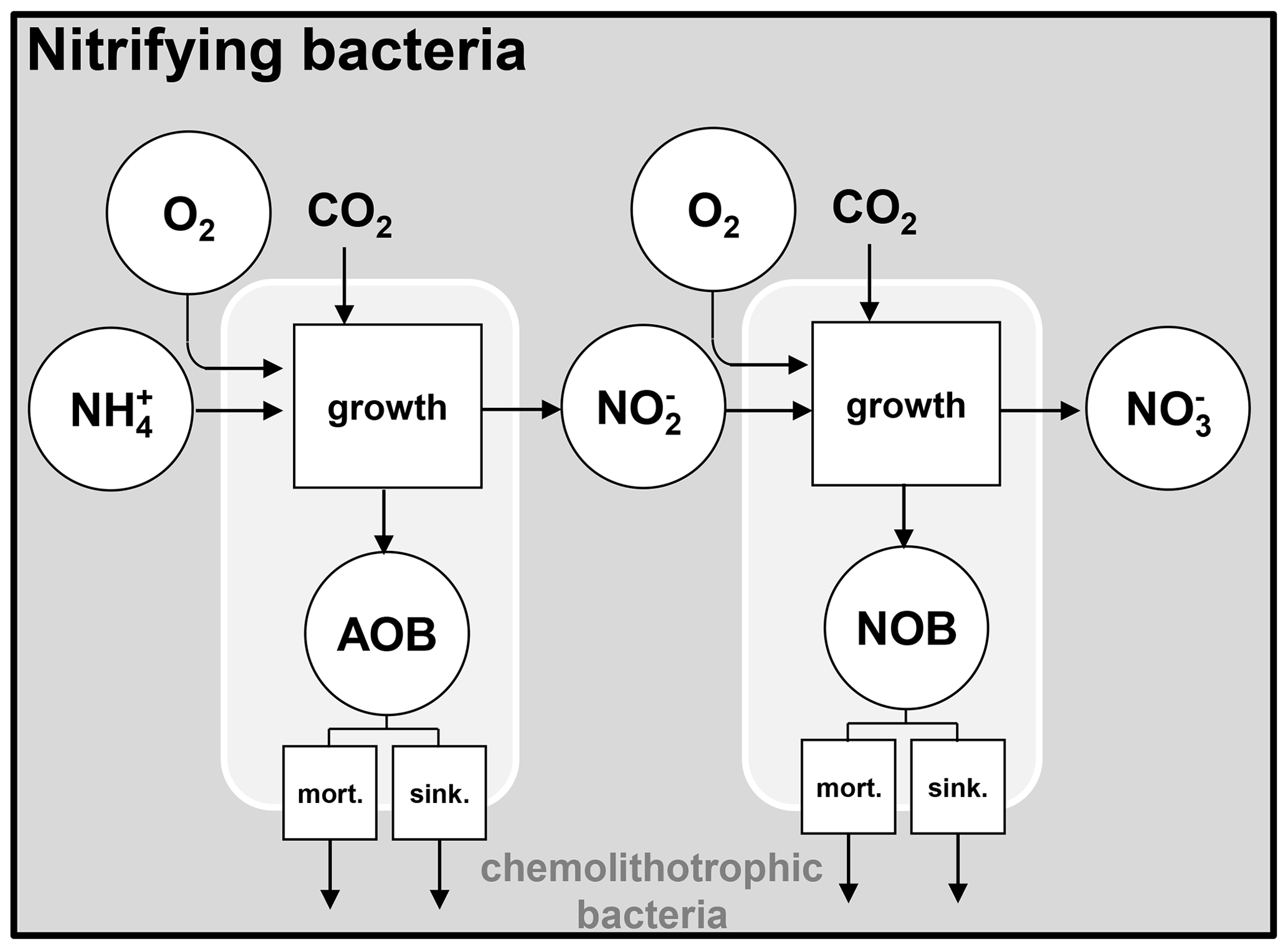
Figure 2 Nitrifying bacteria dynamics. AOB: ammonia-oxidizing bacteria; NOB: nitrite-oxidizing bacteria; mort.: mortality; sink.: sinking.

2.2 Nitrifying bacteria dynamics

The unified RIVE v1.0 model includes the description of the nitrification microbial process, mediated by two types of nitrifying bacteria. They are respectively responsible for the production of nitrite (${\mathrm{NH}}_{\mathrm{4}}^{+}+\frac{\mathrm{3}}{\mathrm{2}}{\mathrm{O}}_{\mathrm{2}}⟶{\mathrm{NO}}_{\mathrm{2}}^{-}+{\mathrm{2}\mathrm{H}}^{+}+{\mathrm{H}}_{\mathrm{2}}\mathrm{O}$) and nitrate (${{\mathrm{NO}}_{\mathrm{2}}}^{-}+\frac{\mathrm{1}}{\mathrm{2}}{\mathrm{O}}_{\mathrm{2}}⟶{\mathrm{NO}}_{\mathrm{3}}^{-}$). The nitrifying bacteria get energy by oxidizing NH${}_{\mathrm{4}}^{+}$ (ammonium) and NO${}_{\mathrm{2}}^{-}$ (nitrite) for their growth. These two bacteria are named AOB (ammonia-oxidizing bacteria) and NOB (nitrite-oxidizing bacteria) (Brion and Billen, 1998). The growth of nitrifying bacteria is limited by the availability of ammonium, nitrite, and oxygen, which is represented with Monod functions (Eq. 7). The effect of water temperature is also taken into account.

$$\begin{array}{}\text{(7)}& {\displaystyle }\begin{array}{rl}{\mathit{\mu }}_{\mathrm{aob}}& ={\mathit{\mu }}_{\max \mathrm{20},\mathrm{aob}}f(T{)}_{\mathrm{aob}}\left({\displaystyle \frac{\left[{\mathrm{NH}}_{\mathrm{4}}^{+}\right]}{\left[{\mathrm{NH}}_{\mathrm{4}}^{+}\right]+K_{{\mathrm{nh}}_{\mathrm{4}},\mathrm{aob}}}}\right)\\ & \left({\displaystyle \frac{\left[{\mathrm{O}}_{\mathrm{2}}\right]}{\left[{\mathrm{O}}_{\mathrm{2}}\right]+K_{{\mathrm{o}}_{\mathrm{2}},\mathrm{aob}}}}\right)\end{array}\text{(8)}& {\displaystyle }\begin{array}{rl}{\mathit{\mu }}_{\mathrm{nob}}& ={\mathit{\mu }}_{\max \mathrm{20},\mathrm{nob}}f(T{)}_{\mathrm{nob}}\left({\displaystyle \frac{\left[{\mathrm{NO}}_{\mathrm{2}}^{-}\right]}{\left[{\mathrm{NO}}_{\mathrm{2}}^{-}\right]+K_{{\mathrm{no}}_{\mathrm{2}},\mathrm{nob}}}}\right)\\ & \left({\displaystyle \frac{\left[{\mathrm{O}}_{\mathrm{2}}\right]}{\left[{\mathrm{O}}_{\mathrm{2}}\right]+K_{{\mathrm{o}}_{\mathrm{2}},\mathrm{nob}}}}\right)\end{array}\end{array}$$

Here, μ_aob and μ_nob are the effective growth rates of AOB and NOB [h⁻¹], μ_max20,aob and μ_max20,nob are the maximal growth rates of AOB and NOB at 20 ^∘C, respectively [h⁻¹], f(T)_aob and f(T)_nob are the water temperature weight at T ^∘C defined as in Eq. (2) [–], $K_{{\mathrm{nh}}_{\mathrm{4}},\mathrm{aob}}$ and $K_{{\mathrm{no}}_{\mathrm{2}},\mathrm{nob}}$ are the half-saturation constants for NH${}_{\mathrm{4}}^{+}$ (AOB) and for NO${}_{\mathrm{2}}^{-}$ (NOB) [mgN L⁻¹], and $K_{{\mathrm{o}}_{\mathrm{2}},\mathrm{aob}}$ and $K_{{\mathrm{o}}_{\mathrm{2}},\mathrm{nob}}$ are the half-saturation constants for oxygen (AOB and NOB) [mgO₂ L⁻¹].

The mortality and sinking of nitrifying bacteria are simulated the same way as for other living species.

$$\begin{array}{}\text{(9)}& {\displaystyle \frac{\mathrm{d}\left[\mathrm{AOB}\right]}{\mathrm{d}t}}=({\mathit{\mu }}_{\mathrm{aob}}-k_{\mathrm{d}\mathrm{20},\mathrm{aob}}f(T{)}_{\mathrm{aob}}-k_{\mathrm{sink},\mathrm{aob}}\left)\right[\mathrm{AOB}]\text{(10)}& {\displaystyle \frac{\mathrm{d}\left[\mathrm{NOB}\right]}{\mathrm{d}t}}=({\mathit{\mu }}_{\mathrm{nob}}-k_{\mathrm{d}\mathrm{20},\mathrm{nob}}f(T{)}_{\mathrm{nob}}-k_{\mathrm{sink},\mathrm{nob}}\left)\right[\mathrm{NOB}]\end{array}$$

Here, μ_aob and μ_nob are the effective growth rates of AOB and NOB defined by Eqs. (7) and (8) [h⁻¹], k_d20,aob and k_d20,nob are the mortality rates of AOB and NOB at 20 ^∘C [h⁻¹], k_sink,aob and k_sink,nob are the sinking rates of AOB and NOB [h⁻¹], f(T)_aob and f(T)_nob are the water temperature weights at T ^∘C defined as in Eq. (2) [–], and [AOB] and [NOB] are the concentrations of AOB and NOB [mgC L⁻¹].

2.3 Primary producer dynamics

The behavior of primary producers is represented using the AQUAPHY model (Lancelot et al., 1991). Biomass of a phytoplankton species is composed of three different cellular constituents (Fig. 3):

• a.

  the structural and functional macromolecules of the cell, F, mainly proteins, chlorophyll, and structural lipids (such as membranes);

• b.

  polysaccharides playing the role of reserve products, R;

• c.

  monomeric (amino acids) and oligomeric precursors for macromolecular synthesis, S.

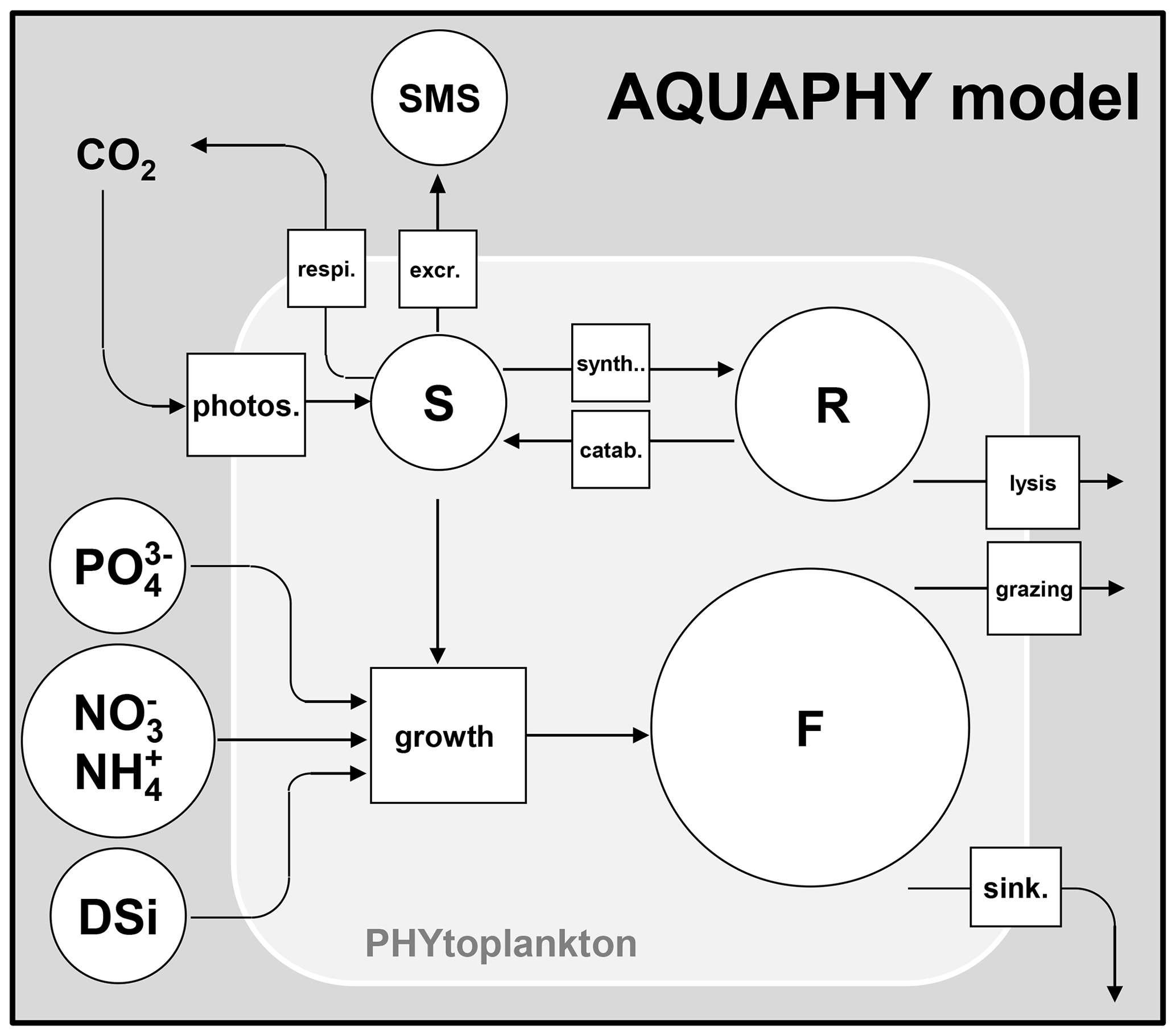
Figure 3 Description of the AQUAPHY model. F: functional macromolecules of the cell; R: reserve products; S: monomeric (amino acids) and oligomeric precursors for macromolecular synthesis. Phytoplankton biomass equals the sum of the three cellular constituents (F, R, S). SMS: small monomeric substrate. photos.: photosynthesis; respi.: respiration; excr.: excretion; synth.: synthesis; catab.: catabolysis; sink.: sinking

At any time, the biomass of the jth phytoplankton species (mgC L⁻¹), [PHY]_j, is equal to the sum of the three internal constituents (Eq. 11), [F]_j, [R]_j, and [S]_j :

$$\begin{array}{}\text{(11)}& [\mathrm{PHY}{]}_j=[\mathrm{F}{]}_j+[\mathrm{R}{]}_j+[\mathrm{S}{]}_j.\end{array}$$

The most common way of measuring phytoplankton biomass is using the chlorophyll a concentration (µg chl a L⁻¹). A carbon to chlorophyll a ratio of 35 mgC µg chl a⁻¹ is therefore considered to convert experimental data into phytoplankton biomass. The initial proportions of different constituents (F, R, S) are fixed (Lancelot et al., 1991). They are only used to determine the initial concentrations of the three cellular constituents and their concentrations in incoming water fluxes for each phytoplankton species. According to Lancelot et al. (1991), the structural and functional macromolecules of the cell ([F]_j) account for about 85 % of the phytoplankton biomass ([PHY]_j), while the reserve products ([R]_j) account for about 10 % of the biomass. The remainder (5 %) of the biomass constitutes the small precursors for macromolecules synthesis ([S]_j). These proportions of F, S, and R are updated at each time step for each phytoplankton species.

2.3.1 Photosynthesis

The photosynthesis process forms small precursors (S) by fixing carbon dioxide. Its rate is determined by the photosynthesis–irradiance relationship (Platt et al., 1980) including three parameters (Eq. 12) and the active irradiance (I(z), µE m⁻² s⁻¹).

$$\begin{array}{}\text{(12)}& \begin{array}{rl}P(z{)}_{{\mathrm{phy}}_j}& =P_{\max \mathrm{20},{\mathrm{phy}}_j}f(T{)}_{{\mathrm{phy}}_j}\\ & \left(\mathrm{1}-e^{-\frac{{\mathit{\alpha }}_{{\mathrm{phy}}_j}I\left(z\right)}{P_{\max \mathrm{20},{\mathrm{phy}}_j}f\left(T\right)}}\right)e^{-\frac{{\mathit{\beta }}_{{\mathrm{phy}}_j}I\left(z\right)}{P_{\max \mathrm{20},{\mathrm{phy}}_j}f\left(T\right)}}\end{array}\end{array}$$

Here, $P(z{)}_{{\mathrm{phy}}_j}$ is the photosynthesis rate of the jth phytoplankton species at water depth z m [h⁻¹], $P_{\max \mathrm{20},{\mathrm{phy}}_j}$ is the maximal photosynthesis rate of the jth phytoplankton species at 20 ^∘C [h⁻¹], $f(T{)}_{{\mathrm{phy}}_j}$ is the water temperature weight of the jth phytoplankton species at T ^∘C defined as in Eq. (2) [–], ${\mathit{\alpha }}_{{\mathrm{phy}}_j}$ is the photosynthetic efficiency of the jth phytoplankton species [h⁻¹ (µE m⁻² s⁻¹)⁻¹], ${\mathit{\beta }}_{{\mathrm{phy}}_j}$ is the photoinhibition capacity of the jth phytoplankton species [h⁻¹ (µE m⁻² s⁻¹)⁻¹], and I(z) is photosynthetically active radiation (PAR) or active irradiance in the water column at depth z m [µE m⁻² s⁻¹] or [W m⁻²].

The averaged photosynthesis rate of the jth phytoplankton species over water column is obtained by integrating P(z):

$$\begin{array}{}\text{(13)}& p_{{\mathrm{phy}}_j}={\displaystyle \frac{{\int }_{\mathrm{0}}^{\mathrm{depth}}P(z{)}_{{\mathrm{phy}}_j}\mathrm{d}z}{\mathrm{depth}}},\end{array}$$

where depth is the water height [m] and $p_{{\mathrm{phy}}_j}$ is the averaged photosynthesis rate over the water column [h⁻¹].

The active irradiance at water depth z m (I(z)) follows the Beer–Lambert law (Eq. 14). The decrease in active irradiance from the water surface to water bottom is represented by the light extinction coefficient (η). The extinction coefficient is composed of three parts: pure water (η_base), suspended solid (η_ss), and algal self-shading (η_chl a).

$$\begin{array}{}\text{(14)}& \begin{array}{rl}& I\left(z\right)=I_{\mathrm{0}}{e}^{-\mathit{\eta }z}\\ & \mathit{\eta }={\mathit{\eta }}_{\mathrm{base}}+{\mathit{\eta }}_{\mathrm{chl}a}\left[\mathrm{chl}a\right]+{\mathit{\eta }}_{\mathrm{ss}}\left[\mathrm{SS}\right]\end{array}\end{array}$$

Here, I(z) is the active irradiance at water depth z [µE m⁻² s⁻¹ or W m⁻²], I₀ is photosynthetically active radiation (PAR) or active irradiance at the water surface measured by the photosynthetic photon¹ flux density (PPFD) [µE m⁻² s⁻¹ or W m⁻²], η is the light extinction coefficient [m⁻¹], η_base is the light extinction coefficient related to pure water [m⁻¹], η_chl a is the linear algal self-shading light extinction coefficient [m⁻¹ (µg chl a L⁻¹)⁻¹], η_ss is the light extinction coefficient related to suspended solid [m⁻¹ (mg L⁻¹)⁻¹], [chl a] is the total chlorophyll a concentration [µg chl a L⁻¹], and [SS] is the suspended solid concentration [mg L⁻¹].

2.3.2 Growth

The growth of phytoplankton involves the transformation of small precursors (S) into structural and functional macromolecules (F), which also requires the uptake of dissolved inorganic nutrients (nitrogen – N, phosphorus – P, silicon – Si) from the environment (Fig. 3). The nutrients can potentially limit phytoplankton growth if their quantities are insufficient. The limitation of nutrients is represented using multiple Monod functions (Eq. 15). The maximum growth rate (${\mathit{\mu }}_{\max ,{\mathrm{F}}_{\mathrm{j}}}$) is itself weighted by a limitation based on the availability of small precursors (S). The limitation by dissolved silica (DSi) is applied only for diatoms (DIA).

$$\begin{array}{}\text{(15)}& {\displaystyle }{\mathit{\mu }}_{{\mathrm{F}}_j}={\mathit{\mu }}_{\max \mathrm{20},{\mathrm{F}}_{\mathrm{j}}}f(T{)}_{{\mathrm{phy}}_j}\left({\displaystyle \frac{\frac{\left[{\mathrm{S}}_j\right]}{\left[{\mathrm{F}}_j\right]}}{\frac{\left[{\mathrm{S}}_j\right]}{\left[{\mathrm{F}}_j\right]}+K_{\mathrm{S},{\mathrm{phy}}_j}}}\right)\mathrm{Nut}\mathit{\_}\lim \text{(16)}& {\displaystyle }\begin{array}{rl}& \mathrm{Nut}\mathit{\_}\lim =\min \left({\displaystyle \frac{\left[\mathrm{DIN}\right]}{\left[\mathrm{DIN}\right]+K_{\mathrm{N},{\mathrm{phy}}_j}}},{\displaystyle \frac{\left[\mathrm{DIP}\right]}{\left[\mathrm{DIP}\right]+K_{\mathrm{P},{\mathrm{phy}}_j}}},\right.\\ & \left.{\displaystyle \frac{\left[\mathrm{DSi}\right]}{\left[\mathrm{DSi}\right]+K_{\mathrm{Si},{\mathrm{phy}}_j}}}\right)\\ & \mathrm{or}\mathrm{Nut}\mathit{\_}\lim =\min \left({\displaystyle \frac{\left[\mathrm{DIN}\right]}{\left[\mathrm{DIN}\right]+K_{\mathrm{N},{\mathrm{phy}}_j}}},{\displaystyle \frac{\left[\mathrm{DIP}\right]}{\left[\mathrm{DIP}\right]+K_{\mathrm{P},{\mathrm{phy}}_j}}}\right)\end{array}\end{array}$$

Here, ${\mathit{\mu }}_{{\mathrm{F}}_j}$ is the effective growth rate of functional macromolecules for the jth phytoplankton species [h⁻¹], ${\mathit{\mu }}_{\max \mathrm{20},{\mathrm{F}}_j}$ is the maximal growth rate of functional macromolecules for the jth phytoplankton species at 20 ^∘C [h⁻¹], $f(T{)}_{{\mathrm{phy}}_j}$ is the water temperature weight of the jth phytoplankton species at T ^∘C defined as in Eq. (2) [–], [S_j] and [F_j] are the concentrations of small precursors and functional macromolecules for the jth phytoplankton species [mgC L⁻¹], $K_{\mathrm{S},{\mathrm{phy}}_j}$ is the half-saturation constant for small precursors of the jth phytoplankton species [–], Nut_lim is the nutrient-limiting factor [–], [DIN], [DIP], and [DSi] are the concentrations of dissolved inorganic nitrogen ($\left[\mathrm{DIN}\right]=\left[{\mathrm{NO}}_{\mathrm{3}}^{-}\right]+\left[{\mathrm{NH}}_{\mathrm{4}}^{+}\right]$, mgN L⁻¹), dissolved inorganic phosphorus ($\left[\mathrm{DIP}\right]=\left[{\mathrm{PO}}_{\mathrm{4}}^{\mathrm{3}-}\right]$, mgP L⁻¹), and dissolved silica (DSi, mgSi L⁻¹), $K_{\mathrm{N},{\mathrm{phy}}_j}$ and $K_{\mathrm{P},{\mathrm{phy}}_j}$ are the half-saturation constants for dissolved inorganic nitrogen and phosphorus of the jth phytoplankton species [mgN L⁻¹ and mgP L⁻¹], and $K_{\mathrm{Si},{\mathrm{phy}}_j}$ is the half-saturation constant for dissolved silica in the case of diatoms [mgSi L⁻¹].

2.3.3 Respiration

The respiration rate of phytoplankton (r_phy) is divided into two components (Eq. 17): one (R_m,phy) ensuring the survival of the cell (maintenance process) and the other (R_μ,phy) corresponding to the energetic cost of growth.

$$\begin{array}{}\text{(17)}& r_{{\mathrm{phy}}_j}=R_{\mathrm{m}\mathrm{20},{\mathrm{phy}}_j}f(T{)}_{{\mathrm{phy}}_j}+{\mathit{\mu }}_{{\mathrm{F}}_j}{R}_{\mathit{\mu },{\mathrm{phy}}_j}\end{array}$$

Here, $r_{{\mathrm{phy}}_j}$ is the respiration rate of the jth phytoplankton species [h⁻¹], $R_{\mathrm{m}\mathrm{20},{\mathrm{phy}}_j}$ is the maintenance respiration rate of the jth phytoplankton species at 20 ^∘C [h⁻¹], $f(T{)}_{{\mathrm{phy}}_j}$ is the water temperature weight of the jth phytoplankton species at T ^∘C defined as in Eq. (2) [–], $R_{\mathit{\mu },{\mathrm{phy}}_j}$ is the respiration for the energetic cost of the jth phytoplankton species [–], and ${\mathit{\mu }}_{{\mathrm{F}}_j}$ is the effective growth rate of the jth phytoplankton species (Eq. 15) [h⁻¹].

2.3.4 Excretion

Included later by Garnier et al. (1998), the phytoplankton excretion (e_phy) includes two terms: a constant excretion rate (E_cst,phy) and another that depends on the photosynthesis rate (E_phot,phy). The product of excretion is the small monomeric substrate (SMS), assimilated directly by heterotrophic bacteria for their growth and respiration (Fig. 1).

$$\begin{array}{}\text{(18)}& e_{{\mathrm{phy}}_j}=E_{\mathrm{cst},{\mathrm{phy}}_j}+p_{{\mathrm{phy}}_j}{E}_{\mathrm{phot},{\mathrm{phy}}_j}\end{array}$$

Here, $e_{{\mathrm{phy}}_j}$ is the excretion rate of the jth phytoplankton species [h⁻¹], $E_{\mathrm{cst},{\mathrm{phy}}_j}$ is the basic excretion rate of the jth phytoplankton species [h⁻¹], $E_{\mathrm{phot},{\mathrm{phy}}_j}$ is the excretion of the jth phytoplankton species related to photosynthesis [–], and $p_{{\mathrm{phy}}_j}$ is the photosynthesis rate of the jth phytoplankton species (Eq. 13) [h⁻¹].

The variation of small monomeric substrate (SMS) can then be established (Eq. 19).

$$\begin{array}{}\text{(19)}& {\displaystyle \frac{\mathrm{d}\left[\mathrm{SMS}\right]}{\mathrm{d}t}}=\mathrm{hydr}-\sum _i{b}_{{\mathrm{hb}}_i}\left[{\mathrm{HB}}_i\right]+\sum _j{e}_{{\mathrm{phy}}_j}\left[{\mathrm{F}}_j\right]\end{array}$$

Here, hydr is the hydrolysis of the dissolved high-weight polymers HD₁ and HD₂ (Eq. 6) [mgC L⁻¹ h⁻¹], $b_{{\mathrm{hb}}_i}$ is the effective rate of substrate uptake by the ith heterotrophic bacteria species (Eq. 3) [h⁻¹], [HB_i] is the biomass concentration of the ith species of heterotrophic bacteria [mgC L⁻¹], $e_{{\mathrm{phy}}_j}$ is the effective excretion rate of the jth phytoplankton species (Eq. 18) [h⁻¹], and [F_j] is the concentration of functional macromolecules for the jth phytoplankton species [mgC L⁻¹].

2.3.5 Synthesis and catabolysis of reserve products

The carbon fixed in the cell by photosynthesis forms small precursors (S) that can be transformed, either into functional macromolecules (F) or into reserve products (R). The synthesis of reserve products is limited by the $\frac{\left[\mathrm{S}\right]}{\left[\mathrm{F}\right]}$ ratio based on a Michaelis–Menten-like function (Eq. 20).

$$\begin{array}{}\text{(20)}& s_{\mathrm{R},{\mathrm{phy}}_j}=s_{\mathrm{R},\max \mathrm{20},{\mathrm{phy}}_j}f(T{)}_{{\mathrm{phy}}_j}{\displaystyle \frac{\frac{\left[{\mathrm{S}}_j\right]}{\left[{\mathrm{F}}_j\right]}}{\frac{\left[{\mathrm{S}}_j\right]}{\left[{\mathrm{F}}_j\right]}+K_{\mathrm{S},{\mathrm{phy}}_j}}}\end{array}$$

Here, $s_{\mathrm{R},{\mathrm{phy}}_j}$ is the synthesis rate of reserve products of jth phytoplankton species [h⁻¹], $s_{\mathrm{R},\max \mathrm{20},{\mathrm{phy}}_j}$ is the maximal synthesis rate of reserve products of jth phytoplankton species at 20 ^∘C [h⁻¹], $f(T{)}_{{\mathrm{phy}}_j}$ is the water temperature weight of jth phytoplankton species at T ^∘C defined as in Eq. (2) [–], [S_j] and [F_j] are the concentrations of small precursors and functional macromolecules for the jth phytoplankton species [mgC L⁻¹], and $K_{\mathrm{S},{\mathrm{phy}}_j}$ is the half-saturation constant for small precursors of the jth phytoplankton species [–].

Reserve products (R) are likely to be catabolized to produce small precursors (S). A first-order kinetic (c_R,phy, h⁻¹) is used to represent catabolysis of a reserve product.

2.3.6 Extinction of phytoplankton

Three ways of phytoplankton extinction are implemented in the unified RIVE v1.0: lysis, sinking, and grazing by zooplankton (Sect. 2.4.1). The phytoplankton lysis is represented by first-order kinetics using a mortality rate (k_d20,phy, h⁻¹). For ease of presentation, all three processes are assumed in an overall extinction rate d_phy (h⁻¹).

$$\begin{array}{}\text{(21)}& \begin{array}{rl}{d}_{{\mathrm{phy}}_j}& =k_{\mathrm{d}\mathrm{20},{\mathrm{phy}}_j}f(T{)}_{{\mathrm{phy}}_j}+k_{\mathrm{sink},{\mathrm{phy}}_j}\\ & +\sum _i{\displaystyle \frac{b_{{\mathrm{zoo}}_i}\left[{\mathrm{ZOO}}_i\right]}{{\sum }_{k=\mathrm{1}}^{\mathrm{NS}}\left[{\mathrm{PHY}}_k\right]}}\end{array}\end{array}$$

Here, $d_{{\mathrm{phy}}_j}$ is the extinction rate of the jth phytoplankton species [h⁻¹], $k_{\mathrm{d}\mathrm{20},{\mathrm{phy}}_j}$ is the mortality rate of the jth phytoplankton species at 20 ^∘C [h⁻¹], $f(T{)}_{{\mathrm{phy}}_j}$ is the water temperature weight of jth phytoplankton species at T ^∘C defined as in Eq. (2) [–], $k_{\mathrm{sink},{\mathrm{phy}}_j}$ is the sinking rate of the jth phytoplankton species [h⁻¹], $b_{{\mathrm{zoo}}_i}$ is the grazing rate of the ith zooplankton species (Eq. 26, Sect. 2.4.1) [h⁻¹], [ZOO_i] is the zooplankton concentration of the ith zooplankton species [mgC L⁻¹], and ${\sum }_{k=\mathrm{1}}^{\mathrm{NS}}\left[{\mathrm{PHY}}_k\right]$ is the total phytoplankton concentration (with NS the number of phytoplankton species grazed by zooplankton) [mgC L⁻¹].

2.3.7 Phytoplankton budgets

According to the processes related to phytoplankton (photosynthesis, growth, mortality, etc.), different budgets can be established for the jth phytoplankton species as follows.

$$\begin{array}{}\text{(22)}& {\displaystyle }\begin{array}{rl}{\displaystyle \frac{\mathrm{d}\left[{\mathrm{S}}_j\right]}{\mathrm{d}t}}& =(p_{{\mathrm{phy}}_j}-r_{{\mathrm{phy}}_j}-{\mathit{\mu }}_{{\mathrm{F}}_j}-s_{\mathrm{R},{\mathrm{phy}}_j})\left[{\mathrm{F}}_j\right]\\ & +c_{\mathrm{R},{\mathrm{phy}}_j}\left[{\mathrm{R}}_j\right]-e_{{\mathrm{phy}}_j}\left[{\mathrm{F}}_j\right]-d_{{\mathrm{phy}}_j}\left[{\mathrm{S}}_j\right]\end{array}\text{(23)}& {\displaystyle \frac{\mathrm{d}\left[{\mathrm{R}}_j\right]}{\mathrm{d}t}}=s_{\mathrm{R},{\mathrm{phy}}_j}\left[{\mathrm{F}}_j\right]-c_{\mathrm{R},{\mathrm{phy}}_j}\left[{\mathrm{R}}_j\right]-d_{{\mathrm{phy}}_j}\left[{\mathrm{R}}_j\right]\text{(24)}& {\displaystyle \frac{\mathrm{d}\left[{\mathrm{F}}_j\right]}{\mathrm{d}t}}=({\mathit{\mu }}_{{\mathrm{F}}_j}-d_{{\mathrm{phy}}_j})\left[{\mathrm{F}}_j\right]\text{(25)}& {\displaystyle }\begin{array}{rl}{\displaystyle \frac{\mathrm{d}\left[{\mathrm{PHY}}_j\right]}{\mathrm{d}t}}& =(p_{{\mathrm{phy}}_j}-r_{{\mathrm{phy}}_j}-e_{{\mathrm{phy}}_j})\left[{\mathrm{F}}_j\right]\\ & -d_{{\mathrm{phy}}_j}\left[{\mathrm{PHY}}_j\right]\end{array}\end{array}$$

Here, $p_{{\mathrm{phy}}_j}$ is the photosynthesis rate of the jth phytoplankton species (Eq. 13) [h⁻¹], $r_{{\mathrm{phy}}_j}$ is the respiration rate of the jth phytoplankton species (Eq. 17) [h⁻¹], ${\mathit{\mu }}_{{\mathrm{F}}_j}$ is the growth rate of the jth phytoplankton species (Eq. 15) [h⁻¹], $s_{\mathrm{R},{\mathrm{phy}}_j}$ is the synthesis rate of reserve products of the jth phytoplankton species (Eq. 20) [h⁻¹], $c_{\mathrm{R},{\mathrm{phy}}_j}$ is the catabolysis rate of reserve products of the jth phytoplankton species [h⁻¹], $e_{{\mathrm{phy}}_j}$ is the excretion rate of the jth phytoplankton species (Eq. 18) [h⁻¹], $d_{{\mathrm{phy}}_j}$ is the extinction rate of the jth phytoplankton species (Eq. 21) [h⁻¹], [S_j], [F_j], and [R_j] are the concentrations of [S_j], [F_j], and [R_j] for the jth phytoplankton species [mgC L⁻¹], and [PHY_j] is the biomass concentration of the jth phytoplankton species [mgC L⁻¹].

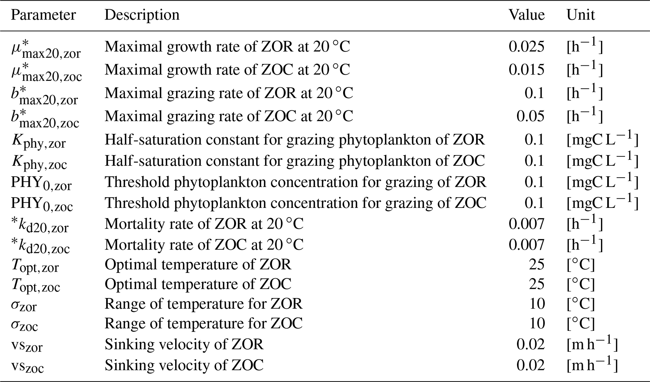
2.4 Zooplankton dynamics

The zooplankton dynamics include grazing on phytoplankton as well as growth, respiration, mortality, and sinking (Fig. 4).

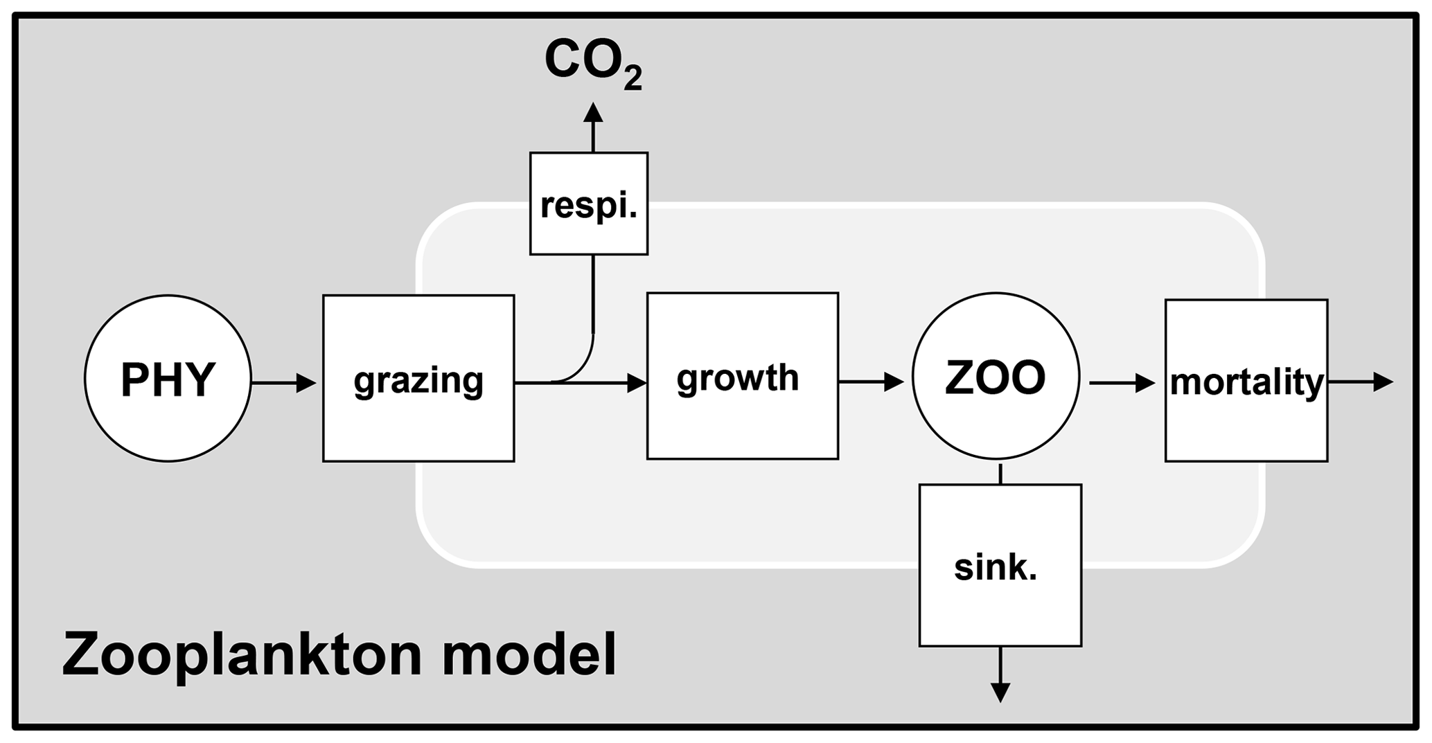
Figure 4 Dynamics of zooplankton. PHY: phytoplankton species; ZOO: zooplankton species; respi.: respiration; sink.: sinking.

2.4.1 Grazing and growth

Grazing on phytoplankton by zooplankton and growth of zooplankton are expressed based on a maximal grazing rate at 20 ^∘C (b_max20,zoo) limited by the phytoplankton biomass based on a Monod function (Eq. 26). The grazing of zooplankton takes place only when the total phytoplankton biomass exceeds a certain threshold ([PHY₀]). No specific preference for grazing on particular phytoplankton species is considered among zooplankton species. Instead, the phytoplankton biomass grazed by the ith species of zooplankton is divided proportionally among each species of phytoplankton (Eq. 21). The growth rate of zooplankton is considered proportional to the grazing rate using a growth yield factor (Eq. 27).

$$\begin{array}{}\text{(26)}& {\displaystyle }\begin{array}{rl}{b}_{{\mathrm{zoo}}_i}& =b_{\max \mathrm{20},{\mathrm{zoo}}_i}f(T{)}_{{\mathrm{zoo}}_i}\\ & {\displaystyle \frac{\left({\sum }_j^{\mathrm{NS}}\left[{\mathrm{PHY}}_j\right]-[{\mathrm{PHY}}_{\mathrm{0}}{]}_{{\mathrm{zoo}}_i}\right)}{\left({\sum }_j^{\mathrm{NS}}\left[{\mathrm{PHY}}_j\right]-[{\mathrm{PHY}}_{\mathrm{0}}{]}_{{\mathrm{zoo}}_i}\right)+K_{\mathrm{phy},{\mathrm{zoo}}_i}}}\end{array}\text{(27)}& {\displaystyle }{\mathit{\mu }}_{{\mathrm{zoo}}_i}=Y_{{\mathrm{zoo}}_i}{b}_{{\mathrm{zoo}}_i}\end{array}$$

Here, $b_{{\mathrm{zoo}}_i}$ is the effective grazing rate of the ith zooplankton species [h⁻¹], $b_{\max \mathrm{20},{\mathrm{zoo}}_i}$ is the maximal grazing rate of the ith zooplankton species at 20 ^∘C [h⁻¹], $f(T{)}_{{\mathrm{zoo}}_i}$ is the water temperature weight of the ith zooplankton species at T ^∘C defined as in Eq. (2) [–], ${\sum }_j^{\mathrm{NS}}\left[{\mathrm{PHY}}_j\right]$ is the total phytoplankton biomass with NS the number of phytoplankton species grazed by zooplankton [mgC L⁻¹], $[{\mathrm{PHY}}_{\mathrm{0}}{]}_{{\mathrm{zoo}}_i}$ is the phytoplankton biomass threshold above which grazing takes place for the ith zooplankton species [mgC L⁻¹], $K_{\mathrm{phy},{\mathrm{zoo}}_i}$ is the half-saturation constant for phytoplankton biomass of the ith zooplankton species [mgC L⁻¹], ${\mathit{\mu }}_{{\mathrm{zoo}}_i}$ is the growth rate of the ith zooplankton species [h⁻¹], and $Y_{{\mathrm{zoo}}_i}$ is the growth yield of the ith zooplankton species [–].

2.4.2 Respiration and mortality

Grazed phytoplankton not used for zooplankton growth is respired (Fig. 4). The rate of respiration is then obtained by $(\mathrm{1}-Y_{\mathrm{zoo}})\times b_{\mathrm{zoo}}$. The mortality of zooplankton is simulated by first-order kinetics (k_d20,zoo).

$$\begin{array}{}\text{(28)}& {\displaystyle }{r}_{{\mathrm{zoo}}_i}=(\mathrm{1}-Y_{{\mathrm{zoo}}_i})\times b_{{\mathrm{zoo}}_i}\text{(29)}& {\displaystyle }\begin{array}{rl}{\displaystyle \frac{\mathrm{d}\left[{\mathrm{ZOO}}_i\right]}{\mathrm{d}t}}& =\left(Y_{{\mathrm{zoo}}_i}{b}_{{\mathrm{zoo}}_i}-k_{\mathrm{d}\mathrm{20},{\mathrm{zoo}}_i}f(T{)}_{{\mathrm{zoo}}_i}\right.\\ & \left.-k_{\mathrm{sink},{\mathrm{zoo}}_i}\right)\left[{\mathrm{ZOO}}_i\right]\end{array}\end{array}$$

Here, $r_{{\mathrm{zoo}}_i}$ is the respiration rate of the ith zooplankton species [h⁻¹], $Y_{{\mathrm{zoo}}_i}$ is the growth yield of the ith zooplankton species [–], $b_{{\mathrm{zoo}}_i}$ is the effective grazing rate of the ith zooplankton species (Eq. 26) [h⁻¹], $k_{\mathrm{d}\mathrm{20},{\mathrm{zoo}}_i}$ is the mortality rate of the ith zooplankton species at 20 ^∘C [h⁻¹], $f(T{)}_{{\mathrm{zoo}}_i}$ is the water temperature weight of the ith zooplankton species at T ^∘C defined as in Eq. (2) [–], $k_{\mathrm{sink},{\mathrm{zoo}}_i}$ is the sinking rate of the ith zooplankton species [h⁻¹], and [ZOO_i] is the biomass concentration of the ith zooplankton species [mgC L⁻¹].

2.5 Nutrient cycling

As shown above, several processes related to nutrients are taken into account: uptake by phytoplankton, mineralization, nitrification, and denitrification (Figs. 5 and 6).

2.5.1 Uptake of nutrients (N, P, Si) by phytoplankton

The Redfield–Conley stoichiometry ($\mathrm{C}:\mathrm{N}:\mathrm{P}:\mathrm{Si}$ $=\mathrm{106}:\mathrm{16}:\mathrm{1}:\mathrm{42}$; – Redfield et al., 1963; Conley et al., 1989) is used to determine the composition of carbon, nitrogen, and phosphorus in organic matter. Constant $\mathrm{C}/\mathrm{N}$, $\mathrm{C}/\mathrm{P}$, and $\mathrm{C}/\mathrm{Si}$ mass ratios are considered to calculate the uptake of nutrients associated with phytoplankton growth.

$$\begin{array}{}\text{(30)}& {\displaystyle \frac{\mathrm{d}\left[\mathrm{uptN}\right]}{\mathrm{d}t}}=\sum _i{\displaystyle \frac{({\mathit{\mu }}_{{\mathrm{F}}_i}+e_{{\mathrm{phy}}_i})\left[{\mathrm{F}}_i\right]}{\mathrm{C}/\mathrm{N}}}\text{(31)}& {\displaystyle }{\mathrm{uptNH}}_{\mathrm{4}}^{+}=\min \left(\right[{\mathrm{NH}}_{\mathrm{4}}^{+}],\mathrm{uptN}{\left({\displaystyle \frac{\left[{{\mathrm{NH}}_{\mathrm{4}}}^{+}\right]}{\left[{{\mathrm{NH}}_{\mathrm{4}}}^{+}\right]+\left[{{\mathrm{NO}}_{\mathrm{3}}}^{-}\right]}}\right)}^{\mathrm{0.025}})\text{(32)}& {\displaystyle }{\mathrm{uptNO}}_{\mathrm{3}}^{-}=\mathrm{uptN}-{\mathrm{uptNH}}_{\mathrm{4}}^{+}\text{(33)}& {\displaystyle \frac{\mathrm{d}\left[\mathrm{uptP}\right]}{\mathrm{d}t}}=\sum _i{\displaystyle \frac{({\mathit{\mu }}_{{\mathrm{F}}_i}+e_{{\mathrm{phy}}_i})\left[{\mathrm{F}}_i\right]}{\mathrm{C}/\mathrm{P}}}\text{(34)}& {\displaystyle \frac{\mathrm{d}\left[\mathrm{uptSi}\right]}{\mathrm{d}t}}={\displaystyle \frac{{\mathit{\mu }}_{\mathrm{F},dia}\left[F_{\mathrm{dia}}\right]}{\mathrm{C}/\mathrm{Si}}}\end{array}$$

Here, ${\mathit{\mu }}_{{\mathrm{F}}_i}$ is the effective growth rate of the ith phytoplankton species (Eq. 15) [h⁻¹], $e_{{\mathrm{phy}}_i}$ is the excretion rate of the ith phytoplankton species (Eq. 18) [h⁻¹], [F_i] represents the functional macromolecule concentration of the ith phytoplankton species [mgC L⁻¹], $\left[{\mathrm{NH}}_{\mathrm{4}}^{+}\right]$ and $\left[{\mathrm{NO}}_{\mathrm{3}}^{-}\right]$ are the concentrations of ammonium and nitrate [mgN L⁻¹], uptN is the uptake of nitrogen for phytoplankton growth [mgN L⁻¹], ${\mathrm{uptNH}}_{\mathrm{4}}^{+}$ is the uptake of NH${}_{\mathrm{4}}^{+}$ for phytoplankton growth [mgN L⁻¹], ${\mathrm{uptNO}}_{\mathrm{3}}^{-}$ is the uptake of NO${}_{\mathrm{3}}^{-}$ for phytoplankton growth [mgN L⁻¹], uptP is the uptake of phosphorus for phytoplankton growth [mgP L⁻¹], $\mathrm{C}/\mathrm{N}$ is the carbon to nitrogen mass ratio [mgC mgN⁻¹], $\mathrm{C}/\mathrm{P}$ is the carbon to phosphorus mass ratio [mgC mgP⁻¹], $\mathrm{C}/\mathrm{Si}$ is the carbon to silica mass ratio [mgC mgSi⁻¹], uptSi is the uptake of silica for diatom growth [mgSi L⁻¹], μ_F,dia is the effective growth rate of diatoms [h⁻¹], and [F_dia] is the functional macromolecule (F) concentration of diatoms [mgC L⁻¹]

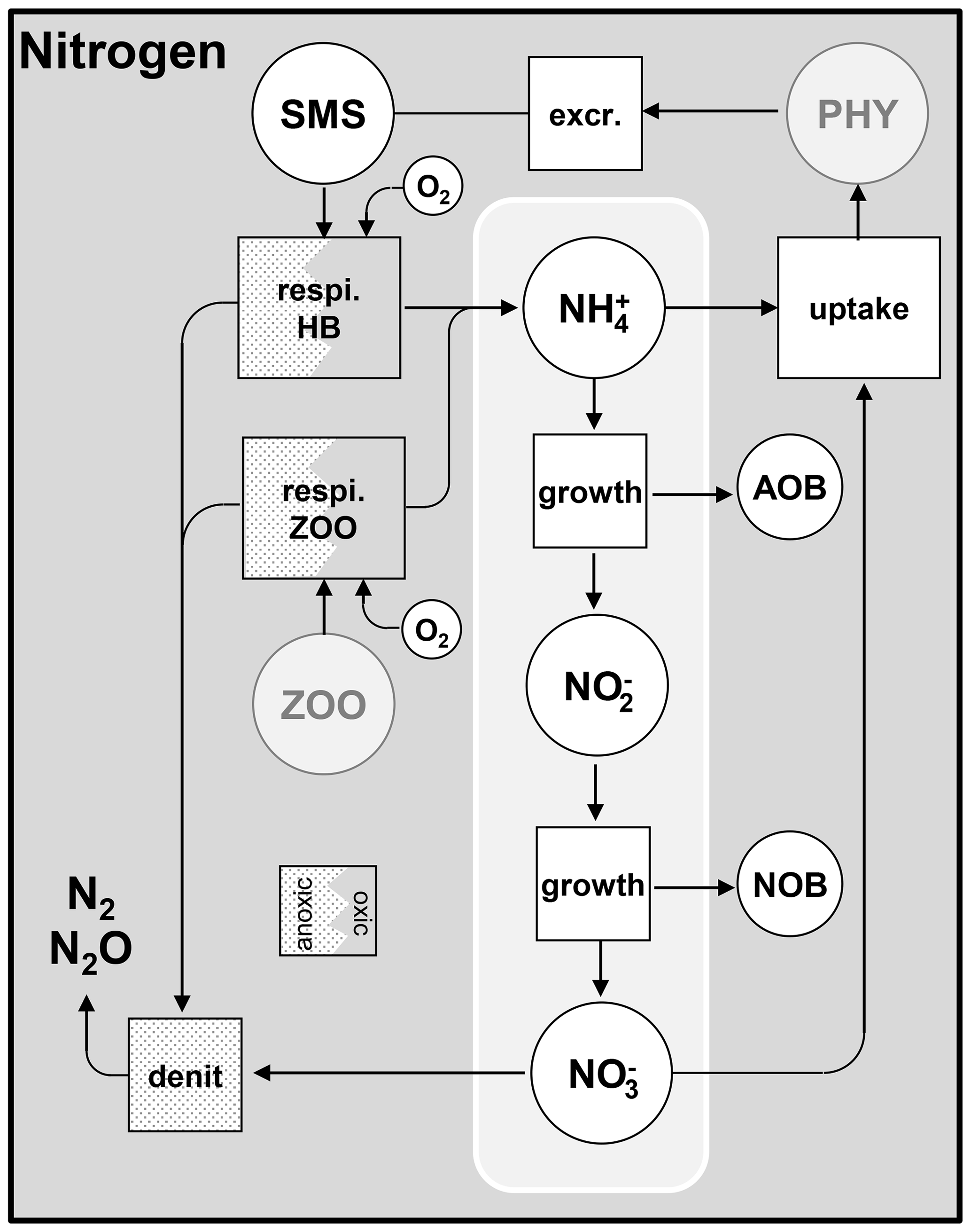
Figure 5 Cycling of nitrogen. PHY: phytoplankton species; HB: heterotrophic bacteria; ZOO: zooplankton species; AOB: ammonia-oxidizing bacteria; NOB: nitrite-oxidizing bacteria; respi.: respiration; excr.: excretion; denit: denitrification.

2.5.2 Release of nutrients by mineralization

The mineralization of organic matter by heterotrophic bacteria and zooplankton is achieved by its oxidation through respiration (Fig. 5). The process consumes organic matter and releases nitrogen and phosphorus from the fraction that is not assimilated for growth of heterotrophic bacteria and zooplankton.

$$\begin{array}{}\text{(35)}& {\displaystyle }\mathrm{respHB}=\sum _i(\mathrm{1}-Y_{{\mathrm{hb}}_i})b_{{\mathrm{hb}}_i}\left[{\mathrm{HB}}_i\right]\text{(36)}& {\displaystyle }\mathrm{respZOO}=\sum _j(\mathrm{1}-Y_{{\mathrm{zoo}}_j})b_{{\mathrm{zoo}}_j}\left[{\mathrm{ZOO}}_j\right]\text{(37)}& {\displaystyle }\mathrm{relN}={\displaystyle \frac{\mathrm{respHB}}{\mathrm{C}/\mathrm{N}}}+{\displaystyle \frac{\mathrm{respZOO}}{\mathrm{C}/\mathrm{N}}}\text{(38)}& {\displaystyle }\mathrm{relP}={\displaystyle \frac{\mathrm{respHB}}{\mathrm{C}/\mathrm{P}}}+{\displaystyle \frac{\mathrm{respZOO}}{\mathrm{C}/\mathrm{P}}}\end{array}$$

Here, respHB is the respiration of heterotrophic bacteria species [mgC L⁻¹ h⁻¹], $Y_{{\mathrm{hb}}_i}$ is the growth yield of the ith heterotrophic bacteria species [–], $b_{{\mathrm{hb}}_i}$ is the effective rate of substrate uptake by the ith heterotrophic bacteria species (Eq. 1) [h⁻¹], [HB_i] is the concentration of the ith heterotrophic bacteria species [mgC L⁻¹], respZOO is the respiration of zooplankton species [mgC L⁻¹ h⁻¹], $Y_{{\mathrm{zoo}}_j}$ is the growth yield of the jth zooplankton species [–], $b_{{\mathrm{zoo}}_j}$ is the effective grazing rate of the jth zooplankton species (Eq. 26) [h⁻¹], [ZOO_j] is the concentration of the jth zooplankton species [mgC L⁻¹], relN is the release of nitrogen [mgN L⁻¹ h⁻¹], $\mathrm{C}/\mathrm{N}$ is the carbon to nitrogen mass ratio [mgC mgN⁻¹], relP is the release of phosphorus [mgP L⁻¹ h⁻¹], and $\mathrm{C}/\mathrm{P}$ is the carbon to phosphorus mass ratio [mgC mgP⁻¹].

2.5.3 Nitrification and denitrification

As mentioned in Sect. 2.2, the nitrification process (Figs. 2 and 5) is related to the growth of AOB (ammonia-oxidizing bacteria) and NOB (nitrite-oxidizing bacteria). Growth yields ($Y_{{\mathrm{aob}}_i}$ and $Y_{{\mathrm{nob}}_j}$) are used to describe the amount of nitrogen consumed by nitrifying bacteria (Eqs. 39 and 40). Denitrification occurs when dissolved oxygen is not present in sufficient quantity (Fig. 5).

$$\begin{array}{}\text{(39)}& {\displaystyle }{\mathrm{nitr}}_{\mathrm{aob}}=\sum _i{\displaystyle \frac{{\mathit{\mu }}_{{\mathrm{aob}}_i}}{Y_{{\mathrm{aob}}_i}}}\left[{\mathrm{AOB}}_i\right]\text{(40)}& {\displaystyle }{\mathrm{nitr}}_{\mathrm{nob}}=\sum _j{\displaystyle \frac{{\mathit{\mu }}_{{\mathrm{nob}}_j}}{Y_{{\mathrm{nob}}_j}}}\left[{\mathrm{NOB}}_j\right]\end{array}$$

Here, ${\mathit{\mu }}_{{\mathrm{aob}}_i}$ and ${\mathit{\mu }}_{{\mathrm{nob}}_j}$ are the effective growth rates of the ith AOB species (Eq. 7) and the jth NOB species (Eq. 8) [h⁻¹], $Y_{{\mathrm{aob}}_i}$ and $Y_{{\mathrm{nob}}_j}$ are the growth yields of the ith AOB species and the jth NOB species [mgC mgN⁻¹], nitr_aob is nitrification calculated as ${\mathrm{NH}}_{\mathrm{4}}^{+}+\frac{\mathrm{3}}{\mathrm{2}}{\mathrm{O}}_{\mathrm{2}}⟶{\mathrm{NO}}_{\mathrm{2}}^{-}+{\mathrm{H}}_{\mathrm{2}}\mathrm{O}+\mathrm{2}{\mathrm{H}}^{+}$ [mgN L⁻¹ h⁻¹], nitr_nob is nitrification calculated as ${\mathrm{NO}}_{\mathrm{2}}^{-}+\frac{\mathrm{1}}{\mathrm{2}}{\mathrm{O}}_{\mathrm{2}}⟶{\mathrm{NO}}_{\mathrm{3}}^{-}$ [mgN L⁻¹ h⁻¹], and [AOB_i] and [NOB_j] are the biomass concentrations of the ith AOB species and the jth NOB species [mgC L⁻¹].

The budgets of ${\mathrm{NO}}_{\mathrm{3}}^{-}$, ${\mathrm{NH}}_{\mathrm{4}}^{+}$, and ${\mathrm{NO}}_{\mathrm{2}}^{-}$ can then be established.

$$\begin{array}{}\text{(41)}& {\displaystyle \frac{\mathrm{d}\left[{\mathrm{NO}}_{\mathrm{3}}^{-}\right]}{\mathrm{d}t}}=-\mathrm{denit}+{\mathrm{nitr}}_{\mathrm{nob}}-{\displaystyle \frac{{\mathrm{uptNO}}_{\mathrm{3}}^{-}}{\mathrm{d}t}}\text{(42)}& {\displaystyle \frac{\mathrm{d}\left[{\mathrm{NH}}_{\mathrm{4}}^{+}\right]}{\mathrm{d}t}}=\mathrm{relN}-{\mathrm{nitr}}_{\mathrm{aob}}-{\displaystyle \frac{{\mathrm{uptNH}}_{\mathrm{4}}^{+}}{\mathrm{d}t}}\text{(43)}& {\displaystyle \frac{\mathrm{d}\left[{\mathrm{NO}}_{\mathrm{2}}^{-}\right]}{\mathrm{d}t}}={\mathrm{nitr}}_{\mathrm{aob}}-{\mathrm{nitr}}_{\mathrm{nob}}\end{array}$$

Here, denit is denitrification [mgN L⁻¹ h⁻¹], nitr_nob is nitrification by NOB (Eq. 40) [mgN L⁻¹ h⁻¹], nitr_aob is nitrification by AOB (Eq. 39) [mgN L⁻¹ h⁻¹], $\frac{{\mathrm{uptNO}}_{\mathrm{3}}^{-}}{\mathrm{d}t}$ is the uptake of NO${}_{\mathrm{3}}^{-}$ by phytoplankton growth (Eq. 32) [mgN L⁻¹ h⁻¹], relN is the release of nitrogen by respiration of heterotrophic bacteria and zooplankton (Eq. 37) [mgN L⁻¹ h⁻¹], and $\frac{{\mathrm{uptNH}}_{\mathrm{4}}^{+}}{\mathrm{d}t}$ is the uptake of NH${}_{\mathrm{4}}^{+}$ by phytoplankton growth (Eq. 31) [mgN L⁻¹ h⁻¹].

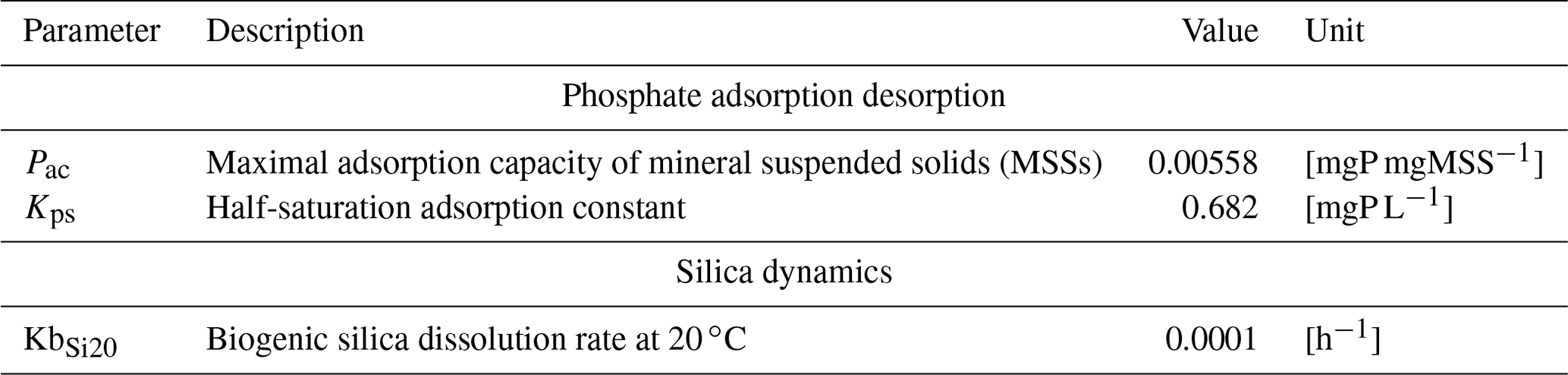
2.5.4 Phosphate adsorption desorption

Orthophosphate (PO${}_{\mathrm{4}}^{\mathrm{3}-}$) is released by mineralization and taken up by phytoplankton exactly as inorganic nitrogen (Fig. 6). Once released in the water column, however, orthophosphates are subject to a process of adsorption–desorption on mineral suspended solids (MSSs) to form PIP (particulate inorganic phosphorus). In addition, the impact of sediment dynamics on P fluxes should be considered in future work with unified RIVE. Vilmin et al. (2015a) showed that P fluxes are mainly driven by hydrological conditions and sediment-related processes in the Seine River system.

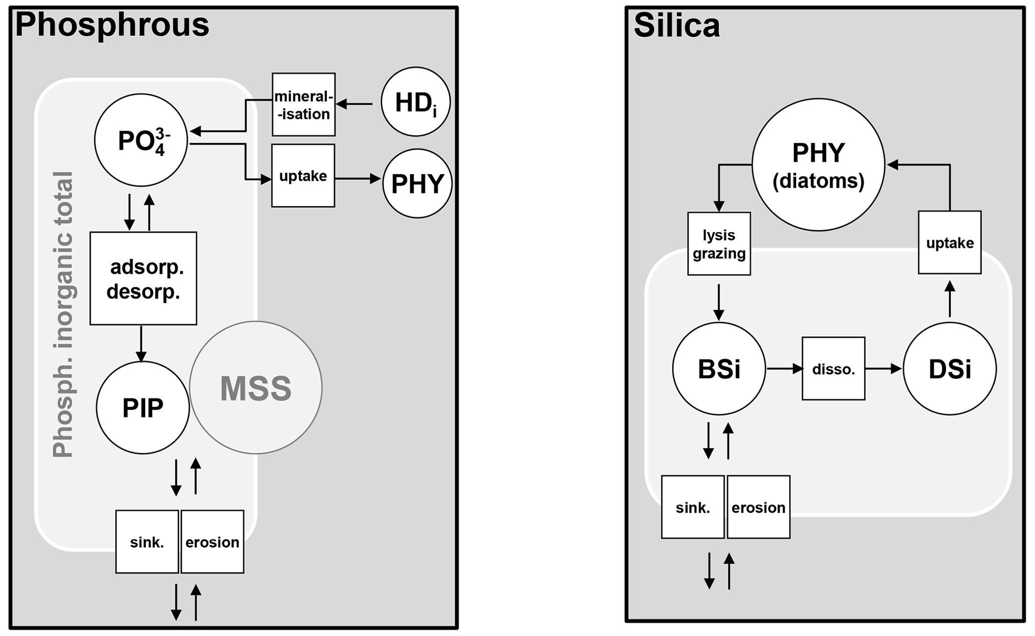
Figure 6 Phosphorus and silica dynamics. HD: dissolved high-weight polymer; PHY: phytoplankton; PIP: particulate inorganic phosphorus; MSS: mineral suspended solids; BSi: biogenic silica; DSi: dissolved silica; adsorp.: adsorption; desorp.: desorption; sink.: sinking; disso. dissolution.

The process is represented according to an instantaneous hyperbolic equilibrium relationship of the form

$$\begin{array}{}\text{(44)}& {\displaystyle \frac{\left[\mathrm{PIP}\right]}{\left[\mathrm{MSS}\right]}}=P_{\mathrm{ac}}\times {\displaystyle \frac{\left[{\mathrm{PO}}_{\mathrm{4}}^{\mathrm{3}-}\right]}{\left[{\mathrm{PO}}_{\mathrm{4}}^{\mathrm{3}-}\right]+K_{\mathrm{ps}}}},\end{array}$$

with $\frac{\left[\mathrm{PIP}\right]}{\left[\mathrm{MSS}\right]}$ the inorganic P content of MSS [mgP mgMSS⁻¹], [PIP] and [MSS] the concentrations of PIP and MSS [mgP L⁻¹ and mgMSS L⁻¹], P_ac the maximum adsorption capacity of MSS [mgP mgMSS⁻¹], $\left[{\mathrm{PO}}_{\mathrm{4}}^{\mathrm{3}-}\right]$ the concentration of orthophosphate [mgP L⁻¹], and K_ps the half-saturation adsorption constant [mgP L⁻¹].

Considering this equilibrium to be instantaneously reached implies that a relationship exists between the variables PIP, MSS, PO${}_{\mathrm{4}}^{\mathrm{3}-}$, and TIP (total inorganic phosphorus):

$$\begin{array}{}\text{(45)}& \left[\mathrm{TIP}\right]=\left[{\mathrm{PO}}_{\mathrm{4}}^{\mathrm{3}-}\right]+\left[\mathrm{PIP}\right].\end{array}$$

This equilibrium relationship can be written as

$$\begin{array}{}\text{(46)}& \left[{\mathrm{PO}}_{\mathrm{4}}^{\mathrm{3}-}\right]={\displaystyle \frac{\begin{array}{c}\left(\left[\mathrm{TIP}\right]-P_{\mathrm{ac}}\times \left[\mathrm{MSS}\right]-K_{\mathrm{ps}}\right)+\\ \sqrt{{\left(-\left[\mathrm{TIP}\right]+P_{\mathrm{ac}}\times \left[\mathrm{MSS}\right]+K_{\mathrm{ps}}\right)}^{\mathrm{2}}+\mathrm{4}\times \left[\mathrm{TIP}\right]\times K_{\mathrm{ps}}}\end{array}}{\mathrm{2}}},\end{array}$$

with $\left[{\mathrm{PO}}_{\mathrm{4}}^{\mathrm{3}-}\right]$ the concentration of orthophosphate [mgP L⁻¹], [TIP] and [MSS] the concentrations of TIP and MSS [mgP L⁻¹ and mgMSS L⁻¹], P_ac the maximal adsorption capacity of MSS [mgP mgMSS⁻¹], and K_ps the half-saturation adsorption constant [mgP L⁻¹].

2.5.5 Silica dynamics

Dissolved silica (DSi) is produced by the dissolution of dead frustules of diatoms (designated as biogenic silica, BSi). Rock weathering contributes also dissolved silica, while it is considered null in unified RIVE v1.0. DSi is taken up by the growth of diatoms (Fig. 6). Biogenic silica is produced by the lysis and grazing of diatoms; it settles down and dissolves according to first-order kinetics, dependent on water temperature (Rickert et al., 2002):

$$\begin{array}{}\text{(47)}& {\displaystyle }{\mathrm{BSi}}_{\mathrm{disso}.}={\mathrm{Kb}}_{\mathrm{Si}}\times \left[\mathrm{BSi}\right],\text{(48)}& {\displaystyle }{\mathrm{Kb}}_{\mathrm{Si}}={\mathrm{Kb}}_{\mathrm{Si}\mathrm{20}}\times {\mathrm{ftp}}_{\mathrm{Si}}\left(T\right),\text{(49)}& {\displaystyle }{\mathrm{ftp}}_{\mathrm{Si}}\left(T\right)=\exp \left({\displaystyle \frac{\mathrm{60}\mathrm{000}}{\mathrm{8.314}}}\times \left({\displaystyle \frac{\mathrm{1}}{\mathrm{275}}}-{\displaystyle \frac{\mathrm{1}}{\mathrm{273}+T}}\right)\right),\end{array}$$

with Kb_Si20 the dissolution rate of biogenic silica at 20 ^∘C [h⁻¹], [BSi] the concentration of biogenic silica [mgSi L⁻¹], and T the water temperature [^∘C].

2.6 Dissolved oxygen

Dissolved oxygen is especially influenced by photosynthesis and respiration. Re-aeration at the water–air interface is also included in the unified RIVE v1.0 model. Sediment dynamics are important for sediment oxygen demand (not shown here). Vilmin et al. (2016) showed that benthic respiration accounts for one-third of the total Seine River respiration. Relevant efforts toward sediment dynamics need to be made in future work, which is not the focus of this study. An oxygen budget can then be established (Eq. 50).

$$\begin{array}{}\text{(50)}& {\displaystyle }\begin{array}{rl}{\displaystyle \frac{\mathrm{d}\left[{\mathrm{O}}_{\mathrm{2}}\right]}{\mathrm{d}t}}& =\mathrm{rea}+{\displaystyle \frac{\mathrm{32}}{\mathrm{12}}}\left(\sum _i\left(p_{{\mathrm{phy}}_i}-r_{{\mathrm{phy}}_i}\right)\left[{\mathrm{F}}_i\right]-\mathrm{respHB}\right.\\ & \left.-\sum _j{r}_{{\mathrm{zoo}}_j}\left[{\mathrm{ZOO}}_j\right]\right)-{\displaystyle \frac{\mathrm{32}}{\mathrm{14}}}\left({\displaystyle \frac{\mathrm{3}}{\mathrm{2}}}{\mathrm{nitr}}_{\mathrm{aob}}+{\displaystyle \frac{\mathrm{1}}{\mathrm{2}}}{\mathrm{nitr}}_{\mathrm{nob}}\right)\end{array}\text{(51)}& {\displaystyle }\mathrm{rea}={\displaystyle \frac{k_{\mathrm{rea}}}{\mathrm{depth}}}\left(\right[{\mathrm{O}}_{\mathrm{2}}{]}_{\mathrm{sat}}-\left[{\mathrm{O}}_{\mathrm{2}}\right])\end{array}$$

Here, k_rea is the re-aeration coefficient [m h⁻¹], “depth” indicates water height [m], [O₂]_sat is the saturated concentration of dissolved oxygen in water [mgO₂ L⁻¹], [O₂] is the concentration of dissolved oxygen in water [mgO₂ L⁻¹], $\frac{\mathrm{32}}{\mathrm{12}}$ is the molar mass ratio between dissolved oxygen and carbon [mgO₂ mgC⁻¹], $p_{{\mathrm{phy}}_i}$ is the photosynthesis rate of the ith phytoplankton species (Eq. 13) [h⁻¹], $r_{{\mathrm{phy}}_i}$ is the respiration rate of the ith phytoplankton species (Eq. 17) [h⁻¹], [F_i] is the functional biomass concentration of the ith phytoplankton species [mgC L⁻¹], respHB is the respiration of all heterotrophic bacteria species (Eq. 35) [mgC L⁻¹ h⁻¹], $r_{{\mathrm{zoo}}_j}$ is the respiration rate of the jth zooplankton species (Eq. 28) [h⁻¹], [ZOO_j] is the biomass concentration of the jth zooplankton species [mgC L⁻¹], $\frac{\mathrm{32}}{\mathrm{14}}$ is the molar mass ratio between dissolved oxygen and nitrogen [mgO₂ mgN⁻¹], nitr_aob is nitrification to produce nitrite by oxidizing ${\mathrm{NH}}_{\mathrm{4}}^{+}$ (Eq. 39, with $\frac{\mathrm{3}}{\mathrm{2}}$ the stoichiometric coefficient) [mgN L⁻¹ h⁻¹], and nitr_nob is nitrification to produce nitrate by oxidizing ${\mathrm{NO}}_{\mathrm{2}}^{-}$ (Eq. 40, with $\frac{\mathrm{1}}{\mathrm{2}}$ the stoichiometric coefficient) [mgN L⁻¹ h⁻¹].

2.7 Inorganic carbon

An inorganic carbon module is implemented in unified RIVE v1.0. The carbonate system is described by a set of equations (named the CO₂ module) based on a previous representation provided by Gypens et al. (2004) and adapted for freshwater environments (Marescaux et al., 2020). In this module, four state variables are defined: dissolved inorganic carbon – DIC, total alkalinity – TA, acidity – pH, and aqueous carbon dioxide – CO₂((aq)).

2.7.1 CO₂ flux at the air–water interface

The DIC is defined as the sum of three dissolved carbonate species:

$$\begin{array}{}\text{(52)}& \left[\mathrm{DIC}\right]=\left[{\mathrm{H}}_{\mathrm{2}}{\mathrm{CO}}_{\mathrm{3}}\right]+\left[{\mathrm{HCO}}_{\mathrm{3}}^{-}\right]+\left[{\mathrm{CO}}_{\mathrm{3}}^{\mathrm{2}-}\right].\end{array}$$

The calculation of pH is derived from Culberson (1980) using TA and DIC. Then the aqueous carbon dioxide (CO₂ (aq)) is derived from the carbonate chemical equilibrium using DIC and pH (Marescaux et al., 2020; Yan et al., 2022a).

$$\begin{array}{}\text{(53)}& \left[{\mathrm{CO}}_{\mathrm{2}}\right(\mathrm{aq}\left)\right]={\displaystyle \frac{\left[\mathrm{DIC}\right]\frac{\left[{\mathrm{H}}^{+}\right]}{K_{\mathrm{1}}}}{\left(\mathrm{1}+\frac{\left[{\mathrm{H}}^{+}\right]}{K_{\mathrm{1}}}+\frac{K_{\mathrm{2}}}{\left[{\mathrm{H}}^{+}\right]}\right)}}\end{array}$$

Here, K₁ and K₂ are the equilibrium constants of carbonate equilibrium reactions (Stumm and Morgan, 1996) [mol L⁻¹], [H⁺] is the concentration of hydrogen ions with pH $=-\log \left(\right[H^{+}\left]\right)$ [mol L⁻¹], and [DIC] is the concentration of dissolved inorganic carbon [mgC L⁻¹].

The flux of CO₂ at the water–air interface ($F_{{\mathrm{CO}}_{\mathrm{2}}}$, gC m⁻² h⁻¹) is calculated based on Fick's first law (Fick, 1855) with a gas transfer velocity of CO₂ ($k_{{\mathrm{CO}}_{\mathrm{2}}}$).

$$\begin{array}{}\text{(54)}& F_{{\mathrm{CO}}_{\mathrm{2}}}=k_{{\mathrm{CO}}_{\mathrm{2}}}\left(\right[{\mathrm{CO}}_{\mathrm{2}}\left(\mathrm{sat}\right)]-[{\mathrm{CO}}_{\mathrm{2}}\left(\mathrm{aq}\right)\left]\right)\end{array}$$

Here, k_co2 is the gas transfer velocity of CO₂ [m h⁻¹], [CO₂(sat)] is the solubility of CO₂ in water calculated based on Henry's law (Weiss, 1974) [mgC L⁻¹], and [CO₂(aq)] is the aqueous carbon dioxide concentration [mgC L⁻¹].

The gas transfer velocity of CO₂ (k_co2) depends on water temperature and k₆₀₀ (gas transfer velocity of CO₂ for a Schmidt number of 600, corresponding to a temperature of 20 ^∘C in freshwater). According to Wilke and Chang (1955), Jähne et al. (1987), and Wanninkhof (1992), the gas transfer velocity of CO₂ (k_co2) at water temperature T (^∘C) can be calculated as

$$\begin{array}{}\text{(55)}& {\displaystyle }{k}_{\mathrm{co}\mathrm{2}}=k_{\mathrm{600}}\sqrt{{\displaystyle \frac{\mathrm{600}}{S{c}_{{\mathrm{CO}}_{\mathrm{2}}}\left(T\right)}}},\end{array}$$

where k₆₀₀ (m h⁻¹) is the gas transfer velocity of CO₂ for a Schmidt number of 600, and $S{c}_{{\mathrm{CO}}_{\mathrm{2}}}\left(T\right)$ is the Schmidt number (dimensionless) calculated with the water temperature in degrees Celsius (^∘C). The $S{c}_{{\mathrm{CO}}_{\mathrm{2}}}\left(T\right)$ can be determined as,=

$$\begin{array}{}\text{(56)}& \begin{array}{rl}S{c}_{{\mathrm{CO}}_{\mathrm{2}}}\left(T\right)& =\mathrm{1911.1}-\mathrm{118.11}T+\mathrm{3.4527}{T}^{\mathrm{2}}\\ & -\mathrm{0.04132}{T}^{\mathrm{3}}.\end{array}\end{array}$$

2.7.2 Budgets of TA and DIC

Processes such as respiration, photosynthesis, nitrification, denitrification, and input flows affect TA and DIC. The unified RIVE v1.0 considers these processes explicitly.

$$\begin{array}{}\text{(57)}& {\displaystyle }\begin{array}{rl}{\displaystyle \frac{\mathrm{dTA}}{\mathrm{d}t}}& =\left[\left({\displaystyle \frac{\mathrm{14}}{\mathrm{106}}}\times {\displaystyle \frac{(\mathrm{respPHY}+\mathrm{respHB}+\mathrm{respZOO})}{\mathrm{12}}}\right)\right.\\ & +{\displaystyle \frac{(\mathrm{denit}-\mathrm{2}\cdot {\mathrm{nitr}}_{\mathrm{aob}})}{\mathrm{14}}}+\left({\displaystyle \frac{\mathrm{17}}{\mathrm{106}}}\times {\displaystyle \frac{{\mathrm{uptNO}}_{\mathrm{3}}^{-}}{\mathrm{uptN}}}-{\displaystyle \frac{\mathrm{15}}{\mathrm{106}}}\right.\\ & \left.\left.\times {\displaystyle \frac{{\mathrm{uptNH}}_{\mathrm{4}}^{+}}{\mathrm{uptN}}}\right)\times {\displaystyle \frac{\sum ({\mathit{\mu }}_{{\mathrm{F}}_i}+e_{{\mathrm{phy}}_i})\left[{\mathrm{F}}_i\right]}{\mathrm{12}}}\right]\\ & \times \mathrm{1000}+{\mathrm{TA}}_{\mathrm{Net}\mathit{\_}\mathrm{Input}}\end{array}\text{(58)}& {\displaystyle }\begin{array}{rl}{\displaystyle \frac{\mathrm{dDIC}}{\mathrm{d}t}}& =(\mathrm{respPHY}+\mathrm{respHB}+\mathrm{respZoo})+\mathrm{denit}\\ & \times {\displaystyle \frac{\mathrm{12}}{\mathrm{14}}}\times {\displaystyle \frac{\mathrm{5}}{\mathrm{4}}}-\sum p_{{\mathrm{phy}}_i}\left[{\mathrm{F}}_i\right]+{\displaystyle \frac{F_{{\mathrm{CO}}_{\mathrm{2}}}}{\mathrm{depth}}}\\ & +{\mathrm{DIC}}_{\mathrm{Net}\mathit{\_}\mathrm{Input}}\end{array}\end{array}$$

Here, TA_{Net_input} (µmol L⁻¹ h⁻¹) and DIC_{Net_input} (mgC L⁻¹ h⁻¹) are the net input fluxes. The respiration of all phytoplankton, bacteria, and zooplankton species (respPHY, respHB, respZOO; mgC L⁻¹ h⁻¹) transforms organic carbon to CO₂ by full oxidization. The denitrification (denit, mgN L⁻¹ h⁻¹) is also considered in the calculation of TA and DIC. $F_{{\mathrm{CO}}_{\mathrm{2}}}$ (gC m⁻² h⁻¹) is the CO₂ flux at the air–water interface, and “depth” is the water depth (m). $\frac{\mathrm{14}}{\mathrm{106}},\frac{\mathrm{17}}{\mathrm{106}},\frac{\mathrm{15}}{\mathrm{106}}$, and $\frac{\mathrm{5}}{\mathrm{4}}$ are the stoichiometry coefficients of biogeochemical processes (Marescaux et al., 2020).

2.8 Kinetic parameters in the unified RIVE model

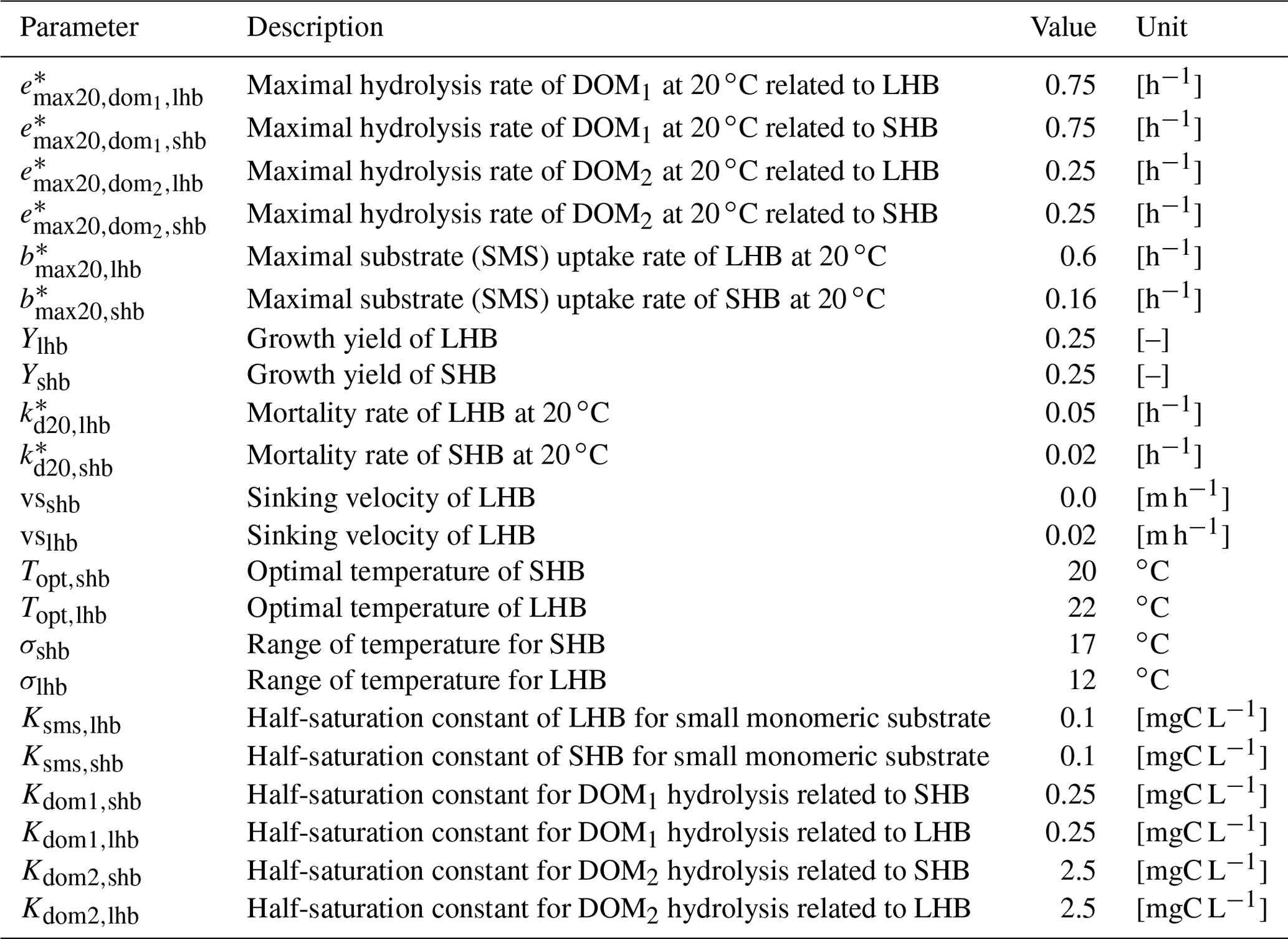
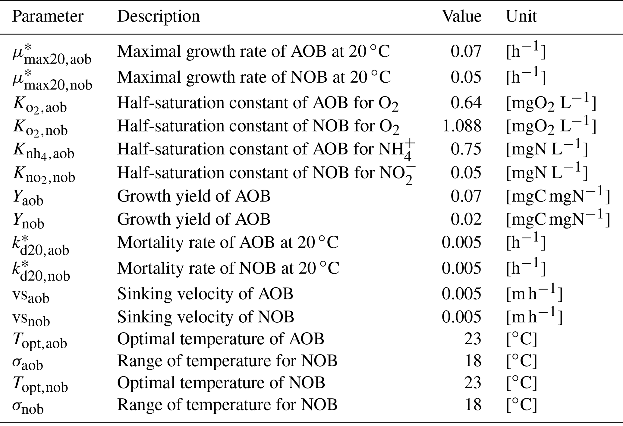
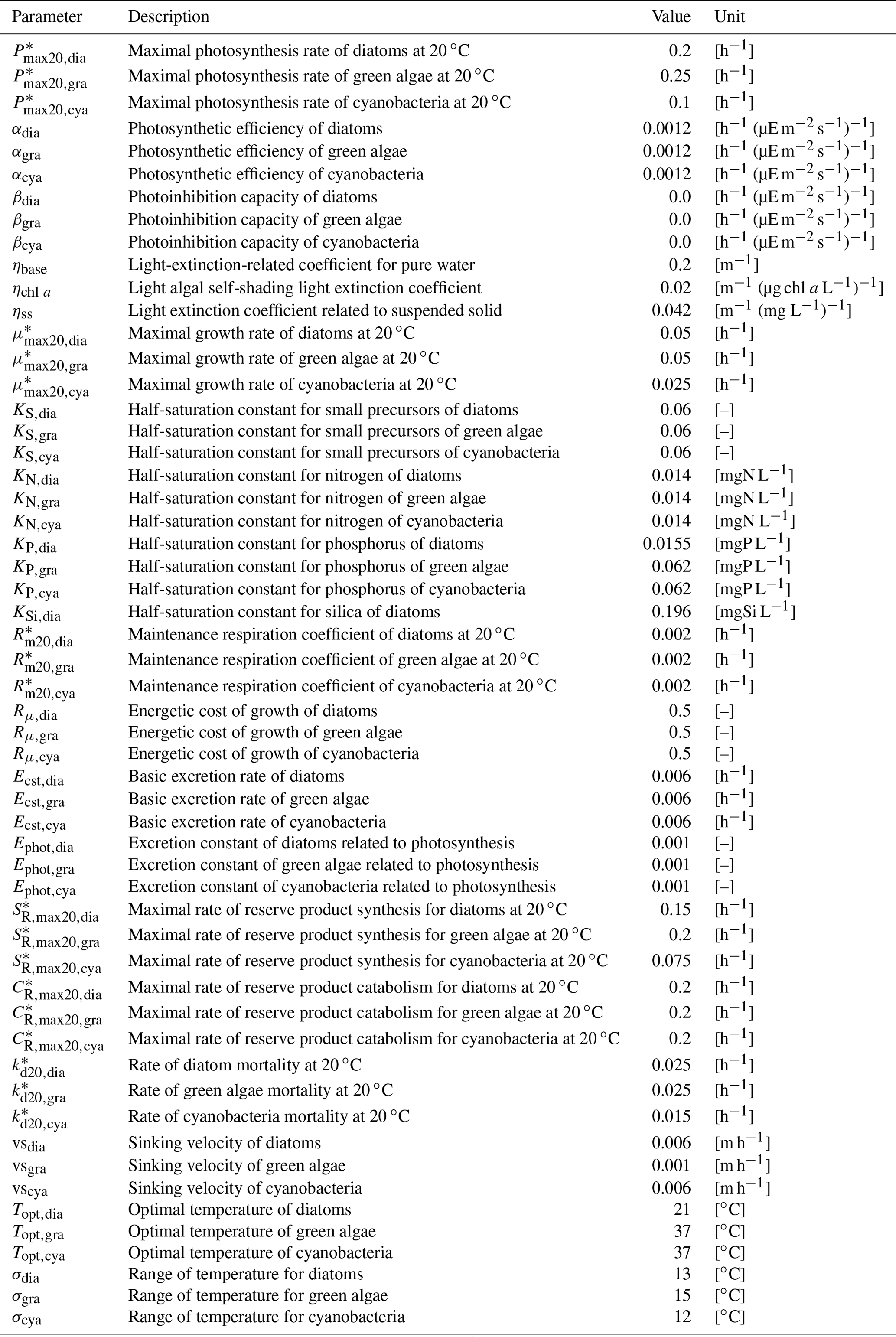
A total of 120 parameters are used to describe the aforementioned processes considering three phytoplankton species and two heterotrophic bacteria species. Some of them depend on water temperature and are calculated with a water temperature function (Eq. 2). Their definitions and reference values are provided in Appendix B.

3 Results

3.1 Digital implementation with Python 3 (pyRIVE 1.0) or ANSI C (C-RIVE 0.32)

The above unified governing equations are implemented in Python 3 to create pyRIVE 1.0 (https://doi.org/10.48579/PRO/Z9ACP1; Thieu et al., 2023) and in ANSI C to create C-RIVE 0.32 (https://doi.org/10.5281/zenodo.7849609; Wang et al., 2023b), respectively. A Jupyter Notebook is used for pedagogical exercises with pyRIVE 1.0, while C-RIVE 0.32 needs to be compiled with gcc under a Linux or a MAC OS operating system. In addition, the user interface of C-RIVE 0.32 uses its own parser based on flex and bison, which allows the software to read ASCII files.

In practice, the number of living species is predefined in pyRIVE 1.0, while we have the ability to define as many species as desired in C-RIVE 0.32 (Table 1). For instance, three communities of phytoplankton (DIA: diatoms; GRA: green algae; CYA: cyanobacteria), two populations of heterotrophic bacteria distinct in their growth rate and size (small one SHB and large one LHB; Garnier et al., 1992a), and two zooplankton communities (ZOR: rotifer and ZOC, micro-crustaceans; Billen et al., 1994; Garnier et al., 1995, 2000) are predefined in pyRIVE 1.0.

In addition, the TIP (total inorganic phosphorus) is considered to be a state variable in pyRIVE 1.0. PO${}_{\mathrm{4}}^{\mathrm{3}-}$ and PIP are derived from it according to Eqs. (45) and (46). TIP is subject to release by heterotrophic bacteria and zooplankton respiration (Eq. 38), uptake by phytoplankton, and settling of PIP together with MSS. However, the PO${}_{\mathrm{4}}^{\mathrm{3}-}$ is treated as a state variable and released by respiration (Eq. 38) in C-RIVE 0.32 and only PIP (particulate inorganic phosphorus) is derived from the Eq. (44).

Table 1 Number of living species defined in pyRIVE 1.0 and C-RIVE 0.32 which implement the unified RIVE v1.0.

Table 2 Initial concentrations and boundary conditions.

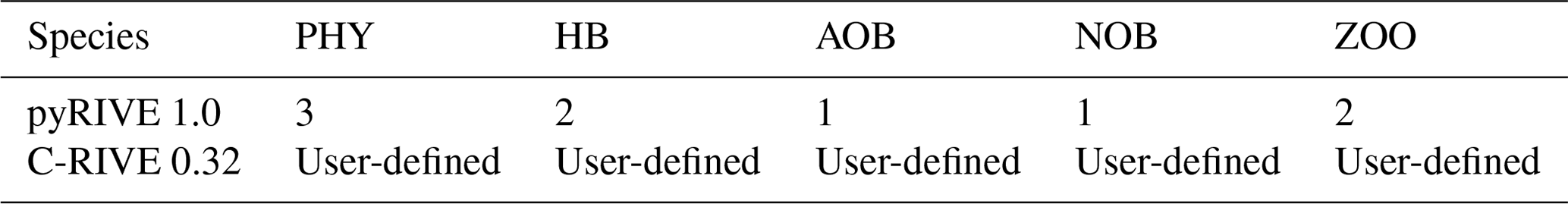
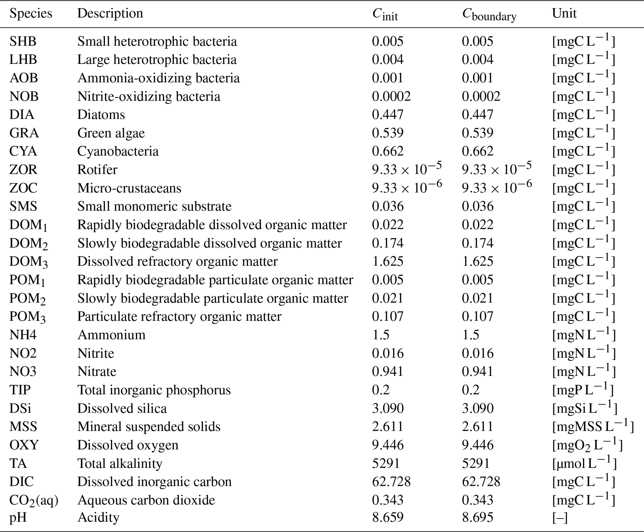
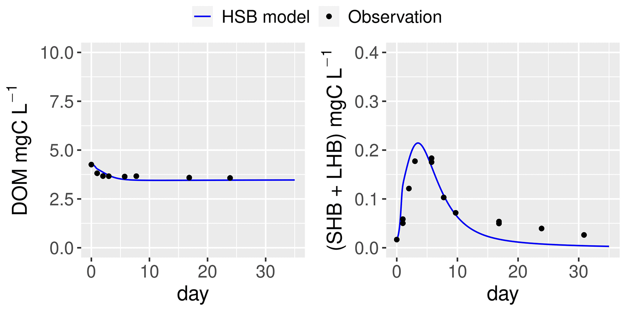
Figure 7 Simulation by the HSB model (unified RIVE v1.0) of the dynamics of heterotrophic bacteria in a filtered and reinoculated sample from drainage pond water (Seine basin, France) taken in February 2021 (Garnier et al., 2021). DOM: dissolved organic matter; SHB: small heterotrophic bacteria.

3.2 Modeling the organic matter degradation by unified RIVE v1.0 (HSB model)

The ability of the HSB model (Fig. 1) to simulate organic matter degradation has been verified by modeling two batch experiments conducted by Garnier et al. (2021). Two water samples were used in the study. One sample was obtained from a drainage pond in the Seine basin, France, in February 2021 (Fig. 7). The other sample was taken from an urban sewage collector in Rosny-sur-Seine, France, in February 2021 (Fig. 8). These samples were incubated in the dark at a temperature of 21 ^∘C for a period of 45 d, during which aerobic bacteria consumed organic matter (Servais et al., 1995). Only DOM and bacterial biomass are measured during batch experiments and then used to show validation. The HSB model is able to effectively reproduce the concentrations of dissolved organic matter and bacterial biomass with a trial–error adjustment of its parameter values (Figs. 7 and 8). The parameter values are kept the same for both water samples.

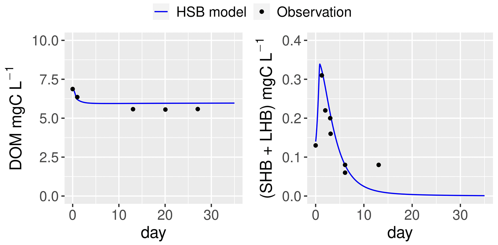
Figure 8 Simulation by the HSB model (unified RIVE v1.0) of the dynamics of heterotrophic bacteria in a filtered and reinoculated sample from urban sewage water (Rosny-sur-Seine, France) taken in February 2021 (Garnier et al., 2021). DOM: dissolved organic matter; SHB: small heterotrophic bacteria; LHB: large heterotrophic bacteria.

Figure 9 Geometric and hydraulic description of a river stretch.

3.3 A river stretch simulated with unified RIVE v1.0: pyRIVE 1.0 vs. C-RIVE 0.32

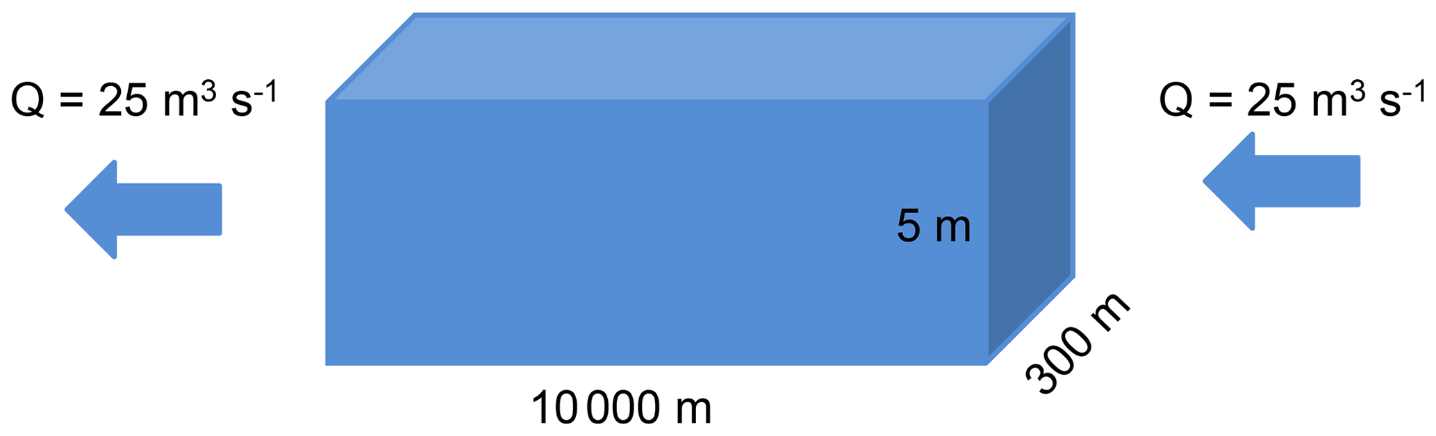
A river stretch with a Strahler order of 8 (Fig. 9) is designed to compare the results simulated by two versions of unified RIVE v1.0 implemented in pyRIVE 1.0 and C-RIVE 0.32. The case study allows us to compare the two versions of unified RIVE v1.0 under transient contrasting conditions (i) between species communities and (ii) temporally for each species community.

3.3.1 River stretch morphology and hydraulic conditions

The stretch measures 10 000 m long and 300 m in width. To simplify the boundary conditions, the upstream inflow and downstream outflow are fixed at 25 m³ s⁻¹, which corresponds to a residence time of 7 d. The water height is fixed at 5 m.

3.3.2 Simulation settings and evaluation strategy

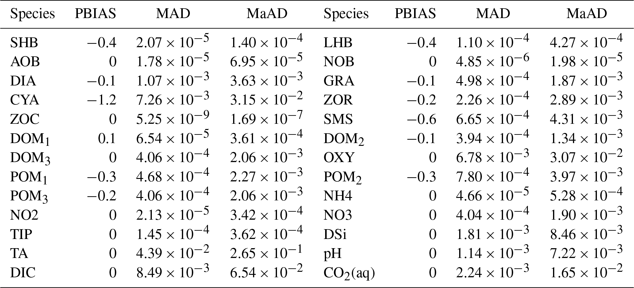
The concentrations of all water quality variables of inflow are defined as their initial concentrations in the stretch and remain constant during the simulation (Table 2). Since this paper focuses on the conceptualization of the unified RIVE v1.0 in the water column, no exchange between the benthic layer and water column is considered. The time step of the simulation is 6 min and a simulation period of 365 d is considered. To compare the results of the two digital implementations of unified RIVE v1.0, daily concentrations at 00:00 are plotted. Three statistical criteria (PBIAS: percent bias, %; MAD: mean absolute difference; MaAD: maximum absolute difference) are calculated to evaluate the similarity of the two sets of results. The closer the criteria are to 0, the more similar the concentrations simulated by the two software packages are (pyRIVE 1.0 and C-RIVE 0.32).

$$\begin{array}{}\text{(59)}& {\displaystyle }\mathrm{PBIAS}=\mathrm{100}{\displaystyle \frac{{\sum }_{i=\mathrm{1}}^N(C_i-{\mathrm{Py}}_i)}{{\sum }_{i=\mathrm{1}}^N{\mathrm{Py}}_i}}\text{(60)}& {\displaystyle }\mathrm{MAD}={\displaystyle \frac{{\sum }_{i=\mathrm{1}}^N|C_i-{\mathrm{Py}}_i|}{N}}\text{(61)}& {\displaystyle }\mathrm{MaAD}=\max \left(\right|C_i-{\mathrm{Py}}_i\left|\right)\end{array}$$

Here, C_i represents the concentrations simulated by C-RIVE 0.32 (in ANSI C) and Py_i those simulated by pyRIVE 1.0 (in Python 3). N is the number of values.

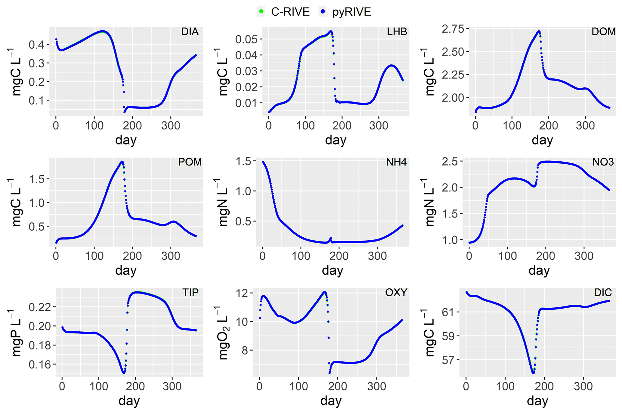
Figure 10 Simulated concentrations of main species by pyRIVE 1.0 and C-RIVE 0.32. See Table 2 for their definitions.

Table 3 Statistical criteria for comparing the simulated variables by pyRIVE 1.0 and C-RIVE 0.32 which implement the unified RIVE v1.0. PBIAS: percent bias [%]; MAD: mean absolute difference; MaAD: maximum absolute The unit of MAD and MaAD depends on the species. It can be [mgC L⁻¹], [mgN L⁻¹], [mgP L⁻¹], [mgSi L⁻¹], or [µmol L⁻¹].

3.3.3 Simulated concentrations of water quality variables

The concentrations simulated by pyRIVE 1.0 and C-RIVE 0.32 are very similar (and superimposed) for all water quality variables (Fig. 10). A maximum absolute difference (MaAD) of 0.0307 mgO₂ L⁻¹, which is relatively low, is obtained for dissolved oxygen concentration. The mean absolute difference (MAD) for dissolved oxygen concentration is 0.00678 mgO₂ L⁻¹ (Table 3) and the corresponding percent bias (PBIAS) is 0 %. The MaAD of 0.0307 mgO₂ L⁻¹ for dissolved oxygen is the cause of the depletion of CYA S (small precursors S of cyanobacteria, Fig. 3) at the beginning of the simulation (not shown here). To correct this depletion of CYA S, the growth of functional macromolecules (CYA F) is reduced according to the availability of CYA S in C-RIVE 0.32. This is why the simulated concentrations of CYA (cyanobacteria) depict a MaAD of 0.0321 mgC L⁻¹ between pyRIVE 1.0 and C-RIVE 0.32. Due to this auto-correction in C-RIVE 0.32, the simulated concentrations of CYA by C-RIVE 0.32 are slightly smaller than those simulated by pyRIVE 1.0 (PBIAS $=-\mathrm{1.2}\mathit{\%}$). The values of PBIAS also indicate the similarity between the concentrations simulated by pyRIVE 1.0 and C-RIVE 0.32. Except for CYA, the discrepancies of other variables are extremely low compared to their concentrations (PBIAS ≤0.6 %). More than half of simulated variables have a PBIAS of 0 %.

4 Discussion

The results show the ability of the unified RIVE v1.0 to correctly simulate the organic matter degradation and the similarity of its two digital implementations (pyRIVE 1.0 and C-RIVE 0.32). Here, we discuss the biogeochemical cycling simulated by unified RIVE v1.0 in the water column (Sect. 4.1), the model limitations, and the future developments (Sect. 4.3), as well as its benefits for the scientific community (Sect. 4.4).

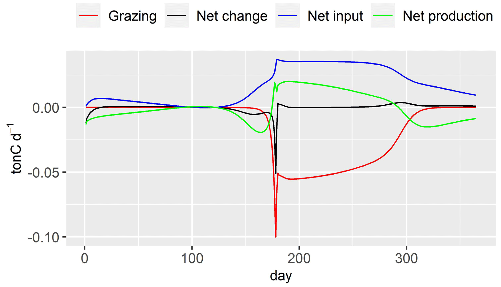
Figure 11 Budget fluxes of DIA (ton C d⁻¹). Grazing: zooplankton grazing fluxes; net production: Eq. (25); net input: input flux–output flux; net change: daily variation of DIA in the river stretch.

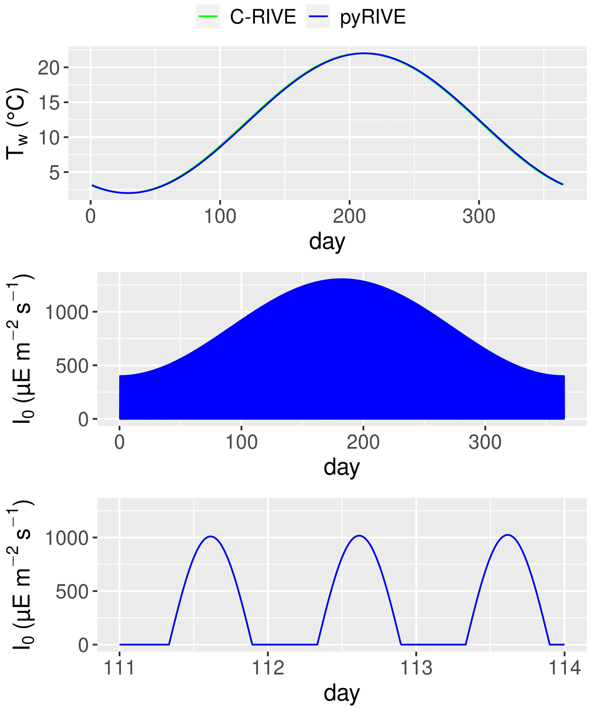
Figure 12 Simulated water temperature, active irradiance, and zoom of active irradiance for days 111–114.

4.1 Biogeochemical cycling in water column simulated by unified RIVE v1.0

The unified RIVE v1.0 simulates the dynamics of microorganisms involving biogeochemical cycling, although the boundary conditions are defined as constant for modeling a river stretch (Fig. 9). Here we interpret the dynamics of diatoms (DIA) and large heterotrophic bacteria (LHB). For this purpose, the budget fluxes of DIA and LHB are calculated.

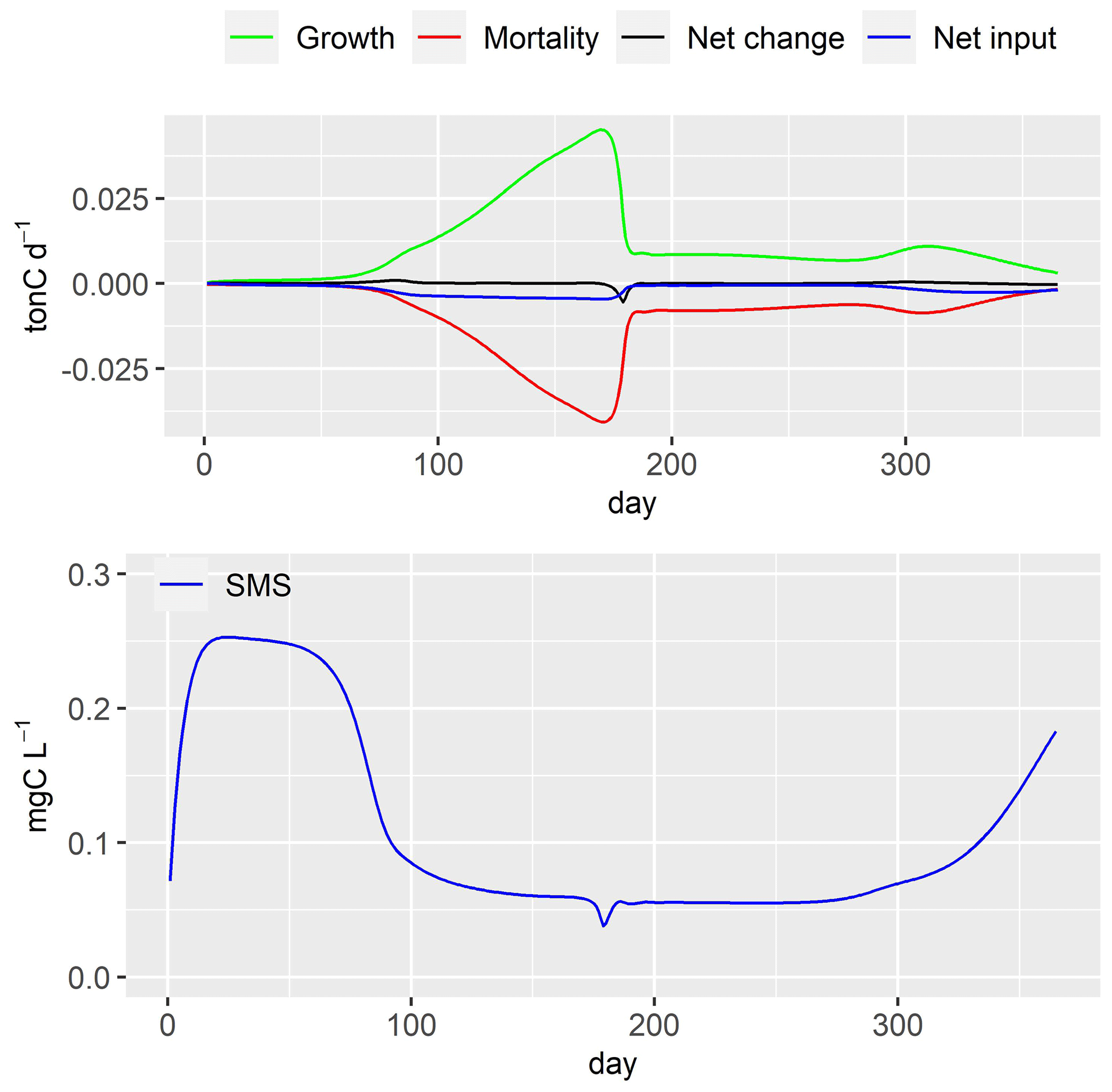
Figure 13 Large heterotrophic bacteria (LHB) dynamics and simulated concentrations of small monomeric substrate (SMS). Net change: daily variation of LHB in river stretch; net input: input flux–output flux.

The decrease in DIA biomass from day 1 to day 15 is related to the low water temperature and low active irradiance, which limit its photosynthesis (Figs. 10, 12). The optimal temperature for the growth of DIA is 21 ^∘C, while the water temperature is lower than 3 ^∘C (Fig. 12). The low photosynthesis rate leads to negative net production (Fig. 11, green line), which is the difference between the fluxes of photosynthesis and the combined fluxes of respiration, mortality, and excretion. During this period, while the input factors play a positive role, the net change in DIA is still negative (Fig. 11, black line). Over the following days, as the water temperature and active irradiance increase (Fig. 12), the net production shows an increase. However, it still remains negative. The net change in DIA shifts to a positive direction due to a combination of net input and net production, leading to a simulated increase in DIA biomass. This trend continues until day 130 when the maximum DIA biomass is reached (Fig. 10). The decline in DIA biomass simulated from day 130 onwards is due to a combination of factors. Firstly, the input factor could be contributing to the decrease when the DIA biomass exceeds the concentration of DIA in input flow (0.447 mgC L⁻¹, Table 2, Fig. 10). Additionally, the net production rate also plays a role (Fig. 11). Although the photosynthesis rate increases with water temperature and active irradiance until day 179 (not shown here), it is not enough to compensate for the other processes occurring in the diatom population (days 150–170), resulting in an overall decrease in biomass. Despite the positive contributions of net input and net production to DIA biomass around day 175, a significant decrease in biomass occurred due to zooplankton grazing (Fig. 11, red line). Two factors impact the zooplankton dynamics: water temperature and the half-saturation constant of grazing (Eq. 26). The optimal temperature for zooplankton is 25 ^∘C and the half-saturation constant of grazing for zooplankton is set to 0.4 mgC L⁻¹. Then, equilibrium of DIA biomass is simulated until day 260 (Fig. 10), which means that the net production and net input in DIA biomass are balanced by the grazing of zooplankton. The input in DIA biomass primarily contributes to the increase in DIA biomass from day 260 (Fig. 11). As the water temperature and active irradiance decrease during this time, the net production of DIA decreases and changes to negative by day 292.

The growth rate of large heterotrophic bacteria (LHB) increases (Fig. 13) with the increase in water temperature, causing a rise in LHB biomass until day 170 (Fig. 10). The fast decrease in small monomeric substrate (SMS) around day 175, synchronized with the grazing of zooplankton (Fig. 11), causes a decrease in growth rate of LHB. Its mortality rate is not impacted (not shown here). Consequently, this leads to a significant reduction in LHB biomass around day 175 (Fig. 10). The biomass of LHB remains stable until day 260. After that, it increases in conjunction with the rise in SMS concentration, which is synchronized with the increase in phytoplankton biomass.

4.2 Complexity and strengths of the RIVE model

Complexity can be understood in terms of the large number of variables represented and interacting with each other. The RIVE model is a multi-element, multi-form model and the kinetics it represents inevitably incorporate a large number of parameters. This is especially true as the RIVE model has opted for an explicit representation of the living communities (bacteria, phytoplankton, zooplankton, etc.) involved in the carbon and nutrient cycles. The model has thus become more complex over time and the addition of new processes (and therefore new parameters) has, as far as possible, been systematically based on experimental work in the laboratory or in the field to reduce the ranges of uncertainty around the kinetic parameters.

The RIVE model is designed as a tool for generating knowledge about the functioning of freshwater ecosystems, and therefore it documents a large number of biogeochemical processes, whether they are expressed weakly or strongly in a given freshwater ecosystem. The underlying hypothesis is that environmental factors control the intensity with which the various processes involved in the overall functioning of a hydrosystem are expressed.

Nevertheless, some work has specifically focused on analyzing the influence of RIVE parameters, particularly those controlling oxygen levels (Wang et al., 2018). This work identified key physical and physiological parameters. Based on the result of sensitivity analysis, a continuous oxygen data assimilation scheme has been developed (Prose-PA, Wang et al., 2019, 2022). The data assimilation allows determining the physiological properties of microorganisms by integrating the associated uncertainties over time. The recent work of Hasanyar et al. (2023) has also helped to better quantify the sensitivity of oxygen to bacterial kinetics parameters as well as those relating to the composition of organic matter with the aim of parsimonious simplification of the number of parameters.

In these two examples, RIVE (C-RIVE) biogeochemical modeling is implemented in much more complex modeling platforms (particle filter, data assimilation, etc.) and the various analyses (sensitivity, uncertainties, etc.) are also supported by an overall assessment of the performance of the model applied to the Seine River.

4.3 Model limitations and future developments of unified RIVE

Currently, the unified RIVE v1.0 presented in this paper describes only the biogeochemical processes in the water column. Comparison of benthic processes and simulations have not been investigated yet. Previous studies showed that sediment plays an important role in the metabolism of river (Vilmin et al., 2016) and lakes (Yan et al., 2022b). A unified sediment module should be further elaborated based on existing modules (Even et al., 2004; Flipo et al., 2004; Thouvenot et al., 2007; Billen et al., 2015; Vilmin et al., 2015b) and implemented into unified RIVE. This sediment module will have to take into account not only the dissolved exchanges between the water column and the sediment but also the resuspension of particulates.

In addition, the unified RIVE v1.0 simulates phytoplankton dynamics, but periphyton or macrophyte development is not implemented in current versions. Flipo et al. (2004) showed that periphyton plays a major role in carbon cycling (primary productivity) in small rivers, not only in the carbon stock fixed at the bottom of the river but also in the carbon enrichment downstream of the river. These limitations should be considered in future developments.

4.4 Benefit of the unified RIVE model

The unified RIVE provides a set of governing equations of freshwater biogeochemical processes across different software platforms, such as pyNuts-Riverstrahler (Billen et al., 1994; Garnier et al., 1995; Thieu et al., 2017), ProSe-PA (Wang et al., 2019, 2023a), SWAT-RIVE (Manteaux et al., 2023), QUAL-NET (Minaudo et al., 2018), VEMALA V3 (Korppoo et al., 2017), and Barman (Garnier et al., 2000; Thieu et al., 2006; Yan et al., 2022b), while incorporating the latest developments. The unity of the kinetics is important for facilitating and reinforcing the collaboration nationally or internationally within different research teams. Thanks to the unity property formerly pointed out by the river continuum concept (Vannote et al., 1980), the software packages based on unified RIVE can leverage the already identified parameter values, regardless of the location in the network (Garnier et al., 2020). This feature is of great interest to the different research teams involved in freshwater quality research, for instance river metabolism (Odum, 1956; Garnier and Billen, 2007; Escoffier et al., 2018; Gurung et al., 2019; Rodríguez-Castillo et al., 2019; Garnier et al., 2020; Segatto et al., 2020; Battin et al., 2023) or nutrient cycling (Garnier et al., 1999b; Alexander et al., 2002; Garnier et al., 2002; Billen et al., 2007; Lauerwald et al., 2013; Lindenschmidt et al., 2019; Maavara et al., 2020; Marescaux et al., 2020; Yan et al., 2022a).

Open science has become increasingly popular and even indispensable in the scientific community as it allows for easier accessibility and the reproduction of scientific results. The unified RIVE project, as an open-source project, allows for the dissemination and wider use of the RIVE biogeochemical model by creating a public repository with different programming languages.

5 Conclusions

This paper presents a conceptual freshwater biogeochemistry model: unified RIVE v1.0, programmed in Python 3 and ANSI C. The degradation of organic matter by heterotrophic bacteria and the dynamics of primary producers (phytoplankton) and zooplankton including carbon cycling and nutrient cycling are described exhaustively. In unified RIVE v1.0, organic matter is degraded via bacteria activity, which is simulated by an HSB model. According to the results, the HSB model is able to model the organic matter degradation and bacterial dynamics in batch experiments. A case study is designed to compare the simulations of the two digital implementations (Python 3 for pyRIVE 1.0 and ANSI C for C-RIVE 0.32). These implementations simulate similar concentrations of all state variables including microorganisms, organic carbon, nutrients, and inorganic carbon.

The river stretch case study allows us to compare the two implementations of unified RIVE V1.0 under transient contrasting conditions involving complex biogeochemical cycles. The specific dynamics of each simulated species depend on different limiting factors. The calculation of photosynthesis of phytoplankton (diatoms, Chlorophyceae, cyanobacteria) takes into account the light that naturally presents a day–night variation. The development of diatoms specifically takes into account the dissolved silica in the simulated environment. The growth of microorganisms depends on the quantity of nutrients (primary producer, nitrifying bacteria) and the small monomeric substrate (heterotrophic bacteria). In addition, the effect of water temperature is also taken into account for the physiology of the simulated microorganism communities (photosynthesis, growth, respiration, mortality).

Finally, unified RIVE being an open-source project, contributions from the freshwater biogeochemistry community are strongly encouraged to achieve a better understanding of freshwater ecosystem functioning and further investigate the future of river systems in a changing world.

Appendix A: Various implementations of the RIVE model and its applications in different freshwater systems

Garnier et al. (2002)Luu et al. (2021)Flipo et al. (2004, 2007)Garnier et al. (2018a)Garnier et al. (2018b)Sferratore et al. (2008)Garnier et al. (1999a)Garnier et al. (2014)Le et al. (2010, 2015); Nguyen et al. (2016)Billen et al. (2005); Thieu et al. (2009)Thieu et al. (2009, 2010)Billen et al. (2007); Thieu et al. (2009, 2010); Romero et al. (2019)Thieu et al. (2017); Desmit et al. (2018); Raimonet et al. (2018); Marescaux et al. (2020)Even et al. (1998, 2004, 2007); Raimonet et al. (2015); Vilmin et al. (2015b, a, 2016, 2018); Wang (2019); Wang et al. (2022)Garnier et al. (2013)Garnier and Billen (1994); Garnier et al. (2000); Thieu et al. (2006); Yan et al. (2022a)

Table A1 Various implementations of the RIVE model and its applications in different freshwater systems.

Appendix B: Parameter values for unified RIVE v1.0

The 120 parameter values necessary for running unified RIVE v1.0 are provided hereafter.

Table B1 Parameters related to heterotrophic bacteria.

^* Parameters depend on water temperature and are multiplied by $f\left(T\right)=\frac{e^{-\frac{(T-T_{\mathrm{opt}}{)}^{\mathrm{2}}}{{\mathit{\sigma }}^{\mathrm{2}}}}}{e^{-\frac{(\mathrm{20}-T_{\mathrm{opt}}{)}^{\mathrm{2}}}{{\mathit{\sigma }}^{\mathrm{2}}}}}$, where T is water temperature in ^∘C.

Table B2 Parameters related to nitrifying bacteria.

^* Parameters depend on water temperature and are multiplied by $f\left(T\right)=\frac{e^{-\frac{(T-T_{\mathrm{opt}}{)}^{\mathrm{2}}}{{\mathit{\sigma }}^{\mathrm{2}}}}}{e^{-\frac{(\mathrm{20}-T_{\mathrm{opt}}{)}^{\mathrm{2}}}{{\mathit{\sigma }}^{\mathrm{2}}}}}$, where T is water temperature in ^∘C.

Table B3 Parameters related to primary producer dynamics.

^* Parameters depend on water temperature and are multiplied by $f\left(T\right)=\frac{e^{-\frac{(T-T_{\mathrm{opt}}{)}^{\mathrm{2}}}{{\mathit{\sigma }}^{\mathrm{2}}}}}{e^{-\frac{(\mathrm{20}-T_{\mathrm{opt}}{)}^{\mathrm{2}}}{{\mathit{\sigma }}^{\mathrm{2}}}}}$, where T is water temperature in ^∘C.

Table B4 Parameters for organic matter dynamics.

^* Parameters depend on water temperature and are multiplied by $f\left(T\right)=\frac{e^{-\frac{(T-T_{\mathrm{opt}}{)}^{\mathrm{2}}}{{\mathit{\sigma }}^{\mathrm{2}}}}}{e^{-\frac{(\mathrm{20}-T_{\mathrm{opt}}{)}^{\mathrm{2}}}{{\mathit{\sigma }}^{\mathrm{2}}}}}$, where T is water temperature in ^∘C.

Table B5 Zooplankton parameters.

^* Parameters depend on water temperature and are multiplied by $f\left(T\right)=\frac{e^{-\frac{(T-T_{\mathrm{opt}}{)}^{\mathrm{2}}}{{\mathit{\sigma }}^{\mathrm{2}}}}}{e^{-\frac{(\mathrm{20}-T_{\mathrm{opt}}{)}^{\mathrm{2}}}{{\mathit{\sigma }}^{\mathrm{2}}}}}$, where T is water temperature in ^∘C.

Table B6 Phosphate- and silica-related parameters.