the Creative Commons Attribution 4.0 License.
the Creative Commons Attribution 4.0 License.
 | 24 May 2024
Simple process-led algorithms for simulating habitats (SPLASH v.2.0): robust calculations of water and energy fluxes
David Sandoval
Iain Colin Prentice
Rodolfo L. B. Nóbrega
The current representation of key processes in land surface models (LSMs) for estimating water and energy balances still relies heavily on empirical equations that require calibration oriented to site-specific characteristics. When multiple parameters are used, different combinations of parameter values can produce equally acceptable results, leading to a risk of obtaining “the right answers for the wrong reasons”, compromising the reproducibility of the simulations and limiting the ecological interpretability of the results. To address this problem and reduce the need for free parameters, here we present novel formulations based on first principles to calculate key components of water and energy balances, extending the already parsimonious SPLASH model v.1.0 (Davis et al., 2017, GMD). We found analytical solutions for many processes, enabling us to increase spatial resolution and include the terrain effects directly in the calculations without unreasonably inflating computational demands. This calibration-free model estimates quantities such as net radiation, evapotranspiration, condensation, soil water content, surface runoff, subsurface lateral flow, and snow-water equivalent. These quantities are derived from readily available meteorological data such as near-surface air temperature, precipitation, and solar radiation, as well as soil physical properties. Whenever empirical formulations were required, e.g., pedotransfer functions and albedo–snow cover relationships, we selected and optimized the best-performing equations through a combination of remote sensing and globally distributed terrestrial observational datasets. Simulations at global scales at different resolutions were run to evaluate spatial patterns, while simulations with point-based observations were run to evaluate seasonal patterns using data from hundreds of stations and comparisons with the VIC-3L model, demonstrating improved performance based on statistical tests and observational comparisons. In summary, our model offers a more robust, reproducible, and ecologically interpretable solution compared to more complex LSMs.
- Article
(29536 KB) - Full-text XML
- BibTeX
- EndNote


Robust representations of water and energy fluxes provide essential foundations for the analysis of interactions and feedbacks within the soil, atmosphere, and vegetation continuum in complex land surface models (LSMs) (Wang et al., 2014; Prentice et al., 2015). These fluxes are greatly shaped by complex topography, which determines the amount of solar energy received at the surface, and by gradients of atmospheric pressure, temperature, and moisture, soil development, and gravitational potential energy, which together control vegetation dynamics and the emergent spatial patterns of ecosystem composition and structure (Tromp-van Meerveld and McDonnell, 2006; Körner, 2021; Sarmiento, 1986). Current models represent the complexity of topographic effects in various simplified ways, for example through discretization of the spatial continuum into hydrological response units (Grayson and Blöschl, 2000; Rodell et al., 2004) or predefined biomes (Liang et al., 1996) or stochastic representation of terrain and land cover at subgrid scales (Lawrence et al., 2019; Liang and Xie, 2001). Or, alternatively, models designed for large-scale applications may simply disregard terrain effects (Davis et al., 2017). This approach has arisen because models typically divide the soil–vegetation–atmosphere column into layers, or small storages, resulting in a large computational demand. So, to run models at higher resolution would increase the required computing power exponentially (Clark et al., 2017).
Although the higher precision of numerical schemes increases the accuracy of the models, the representation of some core hydrological processes still relies on empirical equations that require site-specific calibration (Clark et al., 2017). One outcome of this process is that different combinations of parameter values can produce equally acceptable results, implying a risk of obtaining “the right answers for the wrong reasons” (Grayson and Blöschl, 2000; Prentice et al., 2015), compromising the reproducibility of simulations and limiting the ecological interpretability of the results obtained.
The use of optimization algorithms for multiple parameters in ever more complex models may not necessarily improve matters and, indeed, may hide the inadequacy of concepts such as “field capacity” and “permanent wilting point” when representing one of the most important ecological quantities, the soil water availability to plants. Although these constructs make sense conceptually, they can be misleading. For example, field capacity is described as the remaining water in the soil after drainage has ceased (Kramer and Boyer, 1995; Veihmeyer and Hendrickson, 1931). Still, its value is found in laboratory tests using small soil cores, and it is arbitrarily assumed to be equivalent to the water left after applying 33 kPa of suction (or 10 kPa in sandy soils). The permanent wilting point by definition depends on the plant as well as soil properties. Nonetheless, it is assumed by convention to be equivalent to the water left after applying 1.5 MPa of suction (Kirkham, 2005). Such values are upscaled globally using pedotransfer functions (PTFs), assuming they represent conditions found in nature, but their validity is virtually impossible to test using current LSMs.
The SPLASH model (Davis et al., 2017) is a highly parsimonious, multi-purpose set of algorithms mainly designed for ecohydrological and bioclimatic analysis (see, e.g., Harrison et al., 2010; Gallego-Sala and Prentice, 2012; Ukkola et al., 2015). Even though the original SPLASH assumes a flat cell, neglecting terrain influence on the fluxes, it includes explicit effects of elevation on biophysical quantities with minimum meteorological inputs. At its core, it conceptualizes the daily cycles of water and energy fluxes, and it solves their respective budgets using analytical integrals at a daily time step (Cramer and Prentice, 1988; Davis et al., 2017). We propose new formulations to extend the original SPLASH using theory and concepts based on first principles, thus minimizing the need for free parameters while allowing the representation of processes in complex terrain.
To improve the calculations of the energy fluxes we adapted SPLASH v1.0 mathematical framework to use shortwave radiation as input instead of cloudiness as a proxy for it. Furthermore, we included terrain (slope and aspect) effects on the analytical integrals of the daily energy fluxes and updated the empirical functions used to estimate net longwave radiation.
Since one of the main applications of SPLASH is to infer the water limitation on photosynthesis (Wang et al., 2014; Stocker et al., 2018), we no longer consider the available plant water capacity to be a constant value and added the calculation of subsurface flows. Here, we enhanced SPLASH with an analytical solution for the Green–Ampt equation to calculate daily infiltration, including corrections for slope effects, and analytical solutions for lateral flow, water viscosity effects on hydraulic conductivity, and Dunne and/or Hortonian runoff generation. To upgrade the “bucket model” used in the estimation of soil water content in SPLASH we have included soil hydrophysical properties estimated by PTFs and proposed a theoretical field capacity found by equilibrating gravity with capillarity force. This new version of SPLASH also includes an analytical solution to estimate soil moisture at any depth and a simple snowpack module, which accounts for snowfall occurrence, snow mass balance, and effects on albedo. Processes that still require empirical formulations in the model (i.e., snowfall occurrence, snow albedo feedback, and the effect of soil physical properties on the water retention curve) were optimized using “big data” from remote sensing and in situ measurements.
Some simplifications were adopted in order to allow analytical solutions based on the prevalence of shallow soils and impervious bedrock in mountain regions around the world.
-
The drop of the saturated hydraulic conductivity with depth is neglected.
-
Soil moisture redistribution through the soil profile (down to 2 m) takes no longer than 1 d.
-
Water fluxes in the soil column are in a steady state.
-
The shape of the moisture profile follows Hilberts et al. (2005) and Fan et al. (2007).
-
The snow temperature is 0 °C, so implicitly the energy required to raise the snow temperature is neglected.
The proposed analytical solutions greatly reduce the computational demand compared to numerical schemes, enabling the model to perform calculations using global high-resolution datasets at daily or monthly time steps and to provide emergent spatial patterns of key model outputs such as net radiation, snowpack size, lateral flow, surface runoff, condensation, evapotranspiration, and soil water content.
The inputs of the model are precipitation, solar radiation, and air temperature. To derive terrain information (slope, aspect, and upslope contributing area) the algorithm requires a digital elevation model (DEM) when the grid functionality is used, but, if used with site-specific data (i.e., station data), these variables should be computed beforehand. To estimate some soil hydrophysical properties, the algorithm also requires soil texture, organic matter content, and thickness.
2.1 Energy fluxes
2.1.1 Surface solar radiation
The original formulation for extraterrestrial solar radiation flux I0 (W m−2) from SPLASH (Davis et al., 2017) is defined as
where ISC is the solar constant (W m−2), dr (unitless) is the distance factor, and cos θz is inclination factor. The effects of the slope inclination and orientation on the surface solar radiation were included by using a more complex formulation of cos θz, parameterized after Allen et al. (2006) as follows.
Here, δ (rad) is the declination angle between Earth's Equator and the sun at solar noon and describes the seasonal changes at different latitude ϕ (rad); the hour angle h (rad) describes the sun's position above the horizon, s (rad) is the slope inclination, and γ (rad) is the slope orientation, or aspect, being γ=0 for slopes oriented due south with its values increasing clockwise.
The hour angle when the solar radiation flux reaches the horizon or sunset hour hs was found by replacing Eq. (2) in Eq. (1), setting Io=0, and solving for h.
Furthermore, to simplify the notation, Eq. (3) can be rewritten as
where and . To account for the occurrences of polar days (i.e., no sunset) or polar nights (i.e., no sunrise), hs is set to π when and to zero when , respectively. Here, to approximate the value of sin (hs), the analytical solution proposed by Allen et al. (2006) is used as follows:
where
Note that if we evaluate Eq. (3) for flat surfaces (s=0), it becomes , which is the original SPLASH equation described by Davis et al. (2017).
The daily accumulated incoming radiation (MJ m−2 d−1) is calculated as twice the integral of Eq. (1), with cos (θz(h)) ranging from solar noon (h=0) to sunset (h=hs), times the atmosphere's transmittance τ (unitless).
To exploit datasets of daily average incoming shortwave radiation (SW) (W m−2) and phase out the empirical parameters in the previous model version, which uses the classic Ångström–Prescott formula and cloudiness data, we set H=SW (W m−2) ×86 400 (s d−1) in Eq. (7). Then multiplying both sides of Eq. (7) by (1−βSW), we solve for τ ISC dr (1−βSW) to match the original formulation of the variable rw (W m−2) as follows:
where βSW is the albedo and the other variables are previously defined.
2.1.2 Net surface radiation
The net radiation flux at the surface, IN (W m−2), is defined as the difference between the net shortwave radiation flux, ISW (W m−2), and the net longwave radiation flux, ILW (W m−2),
where ISW is computed simply as the fraction of the incoming shortwave radiation flux not reflected by the albedo, βSW (unitless):
ILW is computed in a similar fashion as the original SPLASH by merging empirical formulations for clear and cloudy skies, both fitted using eddy covariance data from the whole FLUXNET database, thus replacing the old empirical formulations from Monteith and Unsworth (1990) and Linacre (1968) used in the first version.
Here, k1−4 represents empirical coefficients, Tair (°C) is the daily mean near-surface air temperature, and Sf (unitless) is the sunshine fraction, derived from a general form of the Ångström–Prescott equation, with parameters fitted from global databases according to Suehrcke et al. (2013).
Here, k5 and k6 represent empirical coefficients, τ is the atmosphere's transmittance, calculated as the ratio between TOA solar radiation and surface SW data, and τo is the clear-sky atmospheric transmittance, computed following Allen (1996). Values for the coefficients are provided in the Table 1.
Kopp and Lean (2011)Federer (1968)Wang and Zeng (2010); Barry (1996)Linacre (1968)Suehrcke et al. (2013)Suehrcke et al. (2013)Monteith and Unsworth (1990)Monteith and Unsworth (1990)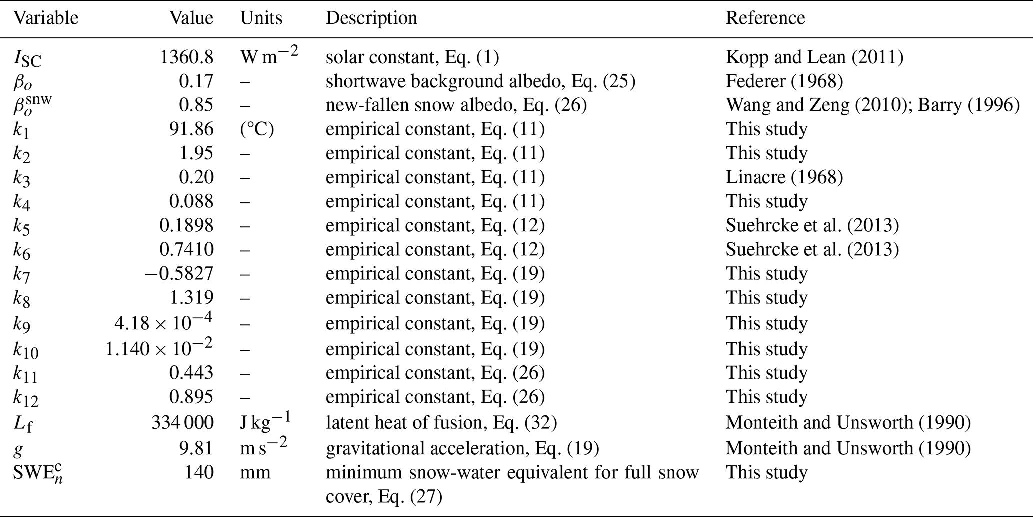
The daily accumulated net radiation, HN (MJ m−2 d−1), is calculated as net positive (daytime approximately) and net negative (nighttime approximately), and the threshold between and is the hour angle when ISW equals ILW (hn) (Fig. 1). It is found by setting IN=0 in Eq. (9) as follows:
For cases where the net radiation is always positive () hn is limited to π, while for the opposite cases, where the net radiation is always negative (), hn is limited to zero.
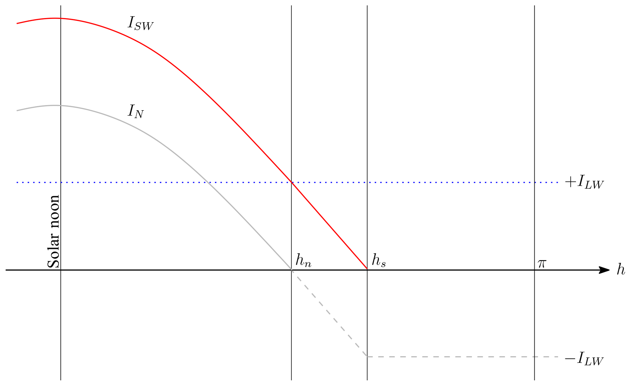
Figure 1Conceptualization of the net radiation flux between solar noon (i.e., h=0) and solar midnight (i.e., h=π) after Davis et al. (2017).
Therefore, as described by Davis et al. (2017), is defined as twice the integral of IN from solar noon to the flux cross-over hour angle hn (Eq. 14), while is calculated as twice the integral of IN between hn and solar midnight (h=π) (Eq. 15).
2.2 Water fluxes and storages
2.2.1 Snowfall
The freezing temperature of the water, 0.0 °C, is the usual threshold to categorize rainfall as snowfall in several models (Pomeroy and Brun, 2001); however, other atmospheric variables like cloudiness, atmospheric pressure, and relative humidity define the snowfall formation (Jennings et al., 2018), therefore changing this temperature threshold in a narrow range across locations (Kienzle, 2008). Here, to get the rainfall–snowfall proportion it is usual to find, among different methods in the literature, linear approximations based on air temperature (Harder and Pomeroy, 2014; Marks et al., 1999; Orth and Seneviratne, 2015) or simply 100 % of the precipitation falling below 0.0 °C assigned as snowfall (Bergström, 1995; Dirmeyer et al., 2006), which might lead to miscalculations in some regions like the Alps, where up to 80 % of its annual precipitation might be in the form of snowfall (Barry, 2008).
Therefore, in the current version of the model a sigmoid curve is used to describe the rain–snow proportion (frain) following Kienzle (2008), who fit empirical equations using 64 years of measurements of rainfall–snowfall proportions from 113 Canadian stations as follows:
where Ttm (°C) is the monthly temperature threshold for the 50 % of rain–snow occurrence, and Trm (°C) is the monthly range of temperatures for snowfall occurrence, both calculated according to Eqs. (17) and (18).
Here, mi is a monthly index (from 1 to 12), and Tr (°C) is the annual range of temperatures for snowfall occurrence, found to be 13 °C as a first approximation by Kienzle (2008). Tt (°C) is the annual threshold for snowfall formation, defined for each year as the annual maximum air temperature when the probability of snowfall occurrence p(snow) equals or exceeds 0.5.
p(snow) was estimated using a binary logistic regression, following the method and datasets provided by Jennings et al. (2018), but reducing the number of explanatory variables to air temperature Tair (°C), elevation z (m a.s.l.), and latitude ϕ (°) as follows (Appendix A4.4):
where , and k10 are coefficients (Table 1). Then, the snowfall is calculated by
2.2.2 Snowmelt
Snowmelt (Sm) (mm d−1) was calculated using a simple relationship between available energy and the size of the snowpack SWE (mm) (snow-water equivalent) as follows:
where SWE is the size of the snowpack expressed as snow-water equivalent (mm), (MJ m−2 d−1) is the daytime accumulated net radiation, ρw (kg m−3) is the water density at 0 °C, Lf (J kg−1) is the latent heat of fusion, and 1000 is the factor to convert m3 to liters. Following Barry (2008), we assumed direct sublimation to be negligible; however, if there is residual energy after the melting occurs, we directed that energy to evaporate Sm, with the flux hereafter denoted simply as “sublimation” (Eswe), which reduces the amount of Sm reaching the soil or producing runoff:
where (MJ m−2 d−1) is the daytime available energy (daytime accumulated net radiation – energy used in melting), Econ (m3 J−1) is the energy-to-water equivalent conversion factor (Davis et al., 2017), and 1000 is the factor to convert m3 to liters. Thus, the water from snowmelt reaching the soil is
2.2.3 Snowpack
The size of the snowpack, expressed as snow-water equivalent SWE (mm), is computed as a simple balance using the previous-day SWE, inputs, and outputs as follows:
The effect of the snow on the albedo was formulated as a simple weighted average using the snow cover fraction, following Wang and Zeng (2010), Roesch and Roeckner (2006), and Niu and Yang (2007),
where βo the is background albedo (Federer, 1968), and βsnw is the snow albedo, calculated according to the age of the snow, following the widely used formulation from the US Army Corps of Engineers (1956).
Here is the albedo of the new-fallen snow, nd is the number of days since a snowfall event greater than 3 mm (Chen et al., 2014), and k11 and k12 are empirical constants. The snow cover fraction (fsnw) from Eq. (25) was estimated using a simple hyperbolic function following Dickinson et al. (1986) and Barry (1996).
Here, SWEc is the snow-water equivalent where fsnw starts to saturate.
The optimized parameters of Eqs. (26) and (27) using remote sensing and ground observations are listed in Table 1.
2.2.4 Infiltration
The infiltration flux rate i (mm h−1) was conceptualized as a two-stage process, which can happen independently or one after another according to the magnitudes of the incoming flux r (mm h−1) (rain and snowmelt) and the infiltration capacity of the soil (Fig. 2).
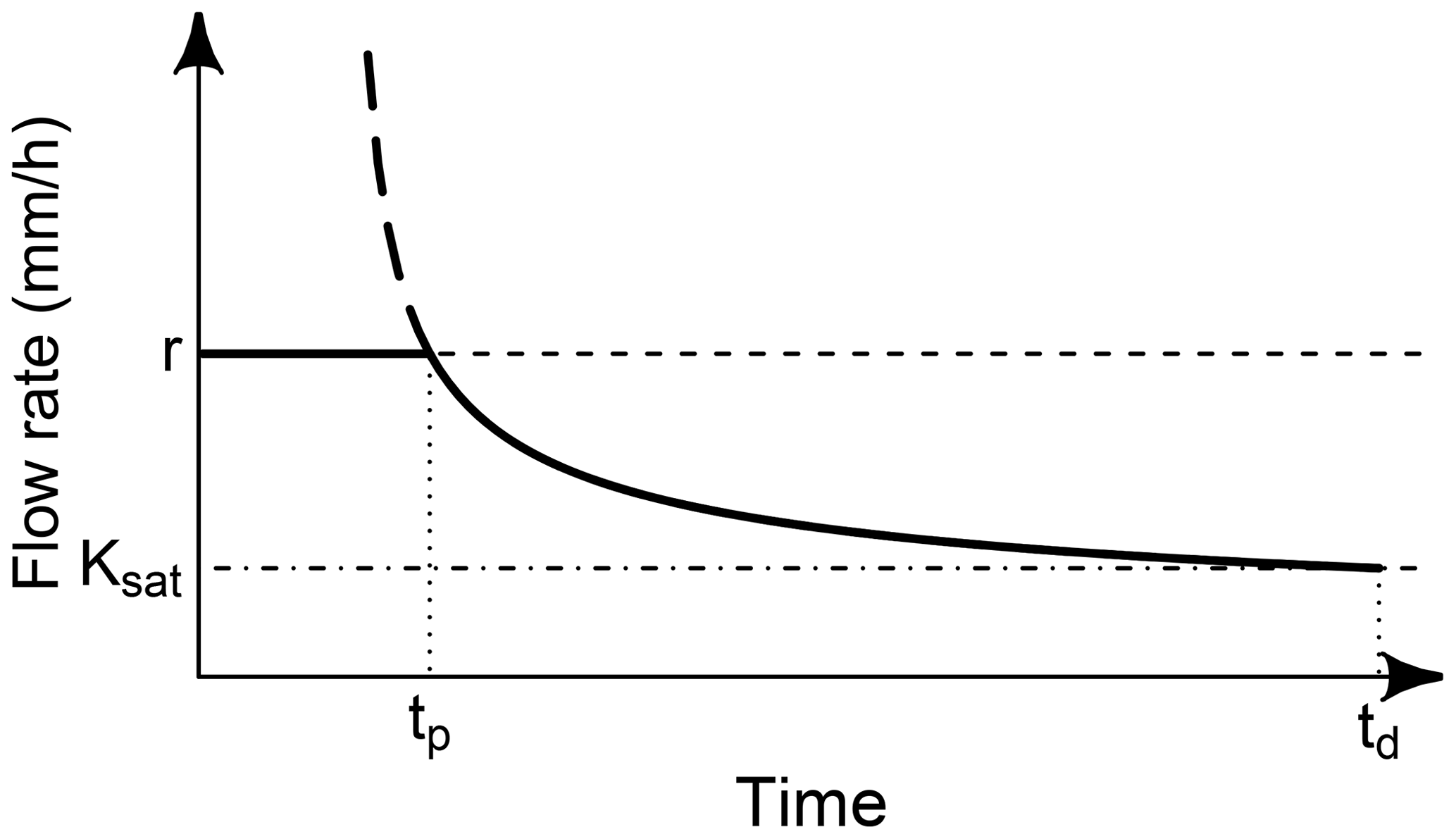
Figure 2Conceptualization of the infiltration process with a constant rainfall r (modified from Tindall et al., 1999). Here, Ksat is the saturated hydraulic conductivity, and tp and td stand for ponding and duration times, respectively.
The first stage, usual when the soil is dry, describes an infiltration rate lower than the infiltration capacity; thus, it is limited by the rainfall and snowmelt rate and lasts until the water flux starts to pond at tp (Vereecken et al., 2019; Assouline, 2013). A second stage describes the system once the water starts to pond on the surface. Here the infiltration rate is limited by the infiltration capacity, which in turn decreases inversely to the water content of the soil, reaching its minimum value (equivalent to Ksat) at saturation following the Green–Ampt formulation, as described by Assouline (2013) and Tindall et al. (1999):
where Ksat (mm h−1) is the saturated hydraulic conductivity, θt,sat (m3 m−3) represents the volumetric soil water content at the time t and at saturation (sat), respectively, I(t) is the cumulative infiltration at the time t, and ψf (mm) is the capillary head at the wetting front, which according to Tindall et al. (1999) is calculated as
with λ being the pore size distribution index (unitless) and ψb (mm) the air-entry pressure, both shaping parameters of the soil water retention curve proposed by Brooks and Corey (1964) (referred to as the BC model hereafter).
Therefore, the ponding time tp can be found by setting Eq. (28) equals to r, which yields
Moreover, to account for the slope (s) effects on tp, the factor is used to reduce tp, following the analysis of Morbidelli et al. (2018); thus, the cumulative infiltration is defined as follows.
Here, td is the duration of the precipitation event, and Δθ is the difference between θsat and the previous θ at the near soil surface, which is calculated using an analytical solution of the Brooks and Corey (1964) model with the previous-day moisture and the depth of the profile (See Sect. 2.7).
The set of equations presented above still requires rainfall intensity and the event's duration to perform the calculations; however, the “minimum inter-event time”, which is used to define a precipitation event, is not consistent in the literature and varies according to the author, location, and application, ranging from 15 min to 24 h (Dunkerley, 2008; Molina-Sanchis et al., 2016), making it difficult to define criteria for global applications. Therefore, as a simplification, an average daily rainfall duration was proposed instead, similar conceptually to the design storm, which is used in calculations for infrastructure design (Smith and Parlange, 1978). In this way, to find the average daily rainfall duration, the daily number of hours with precipitation and the daily precipitation amount were extracted from the Global Satellite Mapping of Precipitation (GsMap v6.0) dataset during the 2000–2014 period (Mega et al., 2014; Yamamoto and Shige, 2015) using the Google Earth Engine (GEE) platform, and the most frequent value was chosen (6 h).
The parameters λ and ψb, which shape the BC model, and Ksat were estimated using pedotransfer functions detailed in Saxton and Rawls (2006), which use soil texture and soil organic matter (SOM) as inputs.
To account for the effects of temperature and atmospheric pressure on the water viscosity and hence on Ksat (Fig. 3), we used the formula described by Hillel (1998):
where ki (m2) is the soil's intrinsic permeability, ρ (kg m−3) is the water density, g (m s−2) is gravitational acceleration, and η (Pa s) is the dynamic viscosity. Thus, we simply used Ksat from the pedotransfer functions, assuming at standard conditions to find ki, which was later replaced in Eq. (32) using actual environmental conditions.
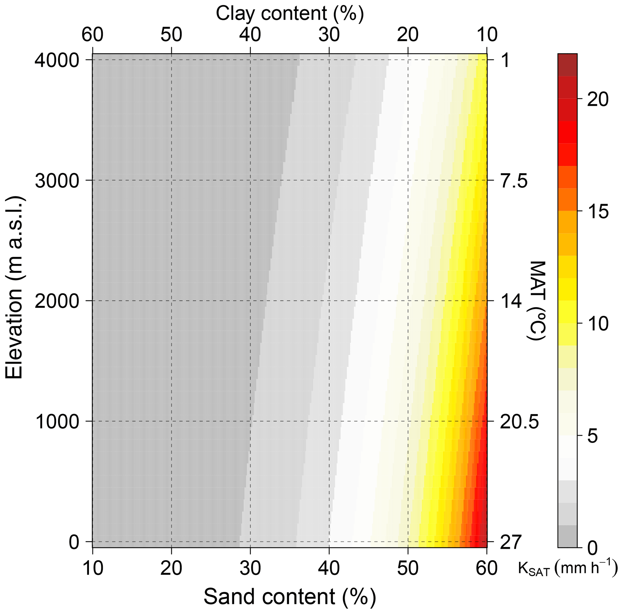
Figure 3Effects of elevation (atmospheric pressure and temperature) on the saturated hydraulic conductivity using a hypothetical soil with 10 % SOM, 30 % silt, and varying sand and clay.
2.2.5 Surface runoff
The runoff formulation considers the different generation mechanisms: the saturation excess overland runoff ROD (mm d−1) (Dunne runoff), which is produced after the soil becomes saturated and is frequent in humid climates or riparian areas (Vereecken et al., 2019), and the infiltration excess overland runoff ROH (mm d−1) (Hortonian runoff), which is produced when the precipitation rate exceeds the infiltration capacity and is more frequent in semi-arid climates (Grayson and Blöschl, 2000; Vereecken et al., 2019):
where r (mm d−1) is water input (rainfall + snowmelt), I (mm d−1) is the infiltration, and Wn,sat (mm) represents the actual and soil water content at saturation, respectively.
Therefore, the daily total RO is simply defined as
2.2.6 Lateral flow
The lateral flow in one cell was defined at steady state as
where qin (mm d−1) is the water draining into the cell from the upslope contributing area and qout (mm d−1) is the water draining out from the cell.
The lateral outgoing flow qout (mm d−1) was conceptualized using some of the TOPMODEL ideas (Beven and Kirby, 1979) on the profile transmissivity (soil hydraulic conductivity K integrated over the soil column) and the hydraulic gradient defined by local topography tan (s) as follows:
where w is the width of the profile's cross-section and Ai is the area of the cell, used here to convert the volumetric flow through the cross-section to equivalent water column units over the cell.
In order to solve the transmittance, the soil moisture distribution through the profile was conceptualized following Hilberts et al. (2005) and Fan et al. (2007) (Fig. 4) with hydrostatic equilibrium at the water table (Remson and Randolph, 1962). Here, the soil moisture redistribution after infiltration was assumed to last less than 1 d within the first 2 m of soil depth, implying a permanent shape of the moisture profile.
Similarly to Fan et al. (2007), due to the lack of information on how Ksat decreases with depth, the model assumes Ksat to be constant through the first 2 m of depth, extending the original 1.5 m proposed by Fan et al. (2007).
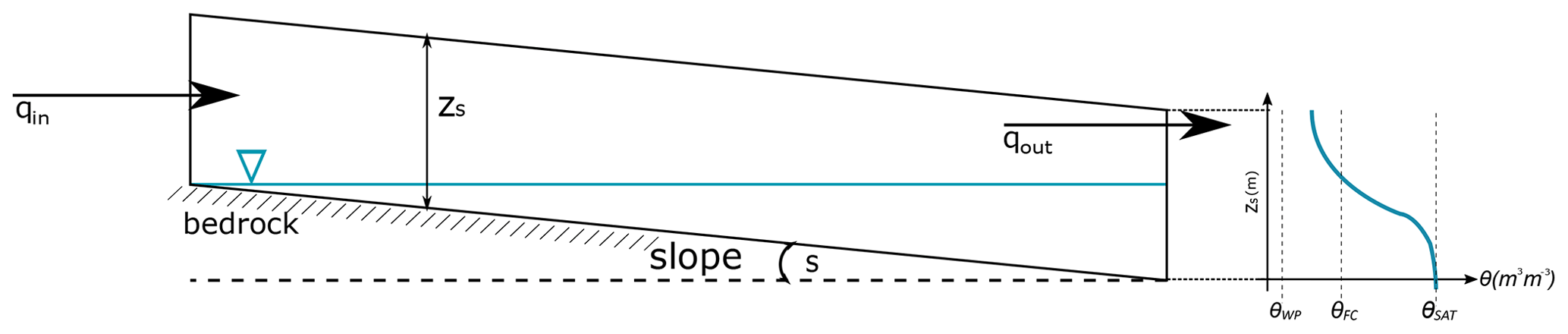
Figure 4Conceptualization of the soil moisture profile in a shallow soil column, after Hilberts et al. (2005) and Fan et al. (2007). We assumed a cell with low spatial resolution and next to a stream.
Therefore, we defined the transmissivity of the profile as the sum of the transmissivities in the unsaturated and saturated parts of the profile as follows:
Thus, to approximate the distribution of θ(z) through the unsaturated part of the soil column, the BC model was used with the total soil water potential (matric+gravitational) after Hino et al. (1988) and Beldring et al. (1999):
where θr (m3 m−3) is the residual soil water content, ψm (mm) is the soil matric potential, and ψg(z) (mm) is the gravitational potential.
The hydraulic conductivity, K(θ) (mm h−1), was defined according to Brooks and Corey (1964) as follows:
Therefore, replacing Eq. (38) in Eq. (39) and solving the integral analytically for the unsaturated part, the transmissivity is defined as
where zwtd (m) is the depth to the water table, found when .
The transmissivity in the saturated part of the profile Tsat is calculated as
The lateral incoming flux qin was formulated using a simple linear reservoir model (Buytaert et al., 2004; Yang et al., 2018; Vogel and Kroll, 1996), with a decaying volumetric flux as a function of time:
where Qf is the final flux after the time t and Qo (m3 d−1) is the initial volumetric flow soon after the precipitation event. If we set the cease of drainage at field capacity we get
where Qfc (m3 d−1) is the volumetric flow after the time t (d), and Kb is the recession constant (unitless), which was found using the drainable porosity; see Appendix A. Therefore, the total volume result of a daily (1 d) recharge (R>0) over the upslope area (Fig. 5), theoretically, can be approximated by
where Au is the upslope area (m2), R is the recharge (mm d−1), which is defined as infiltration minus evapotranspiration and t0 is the time at Qo.
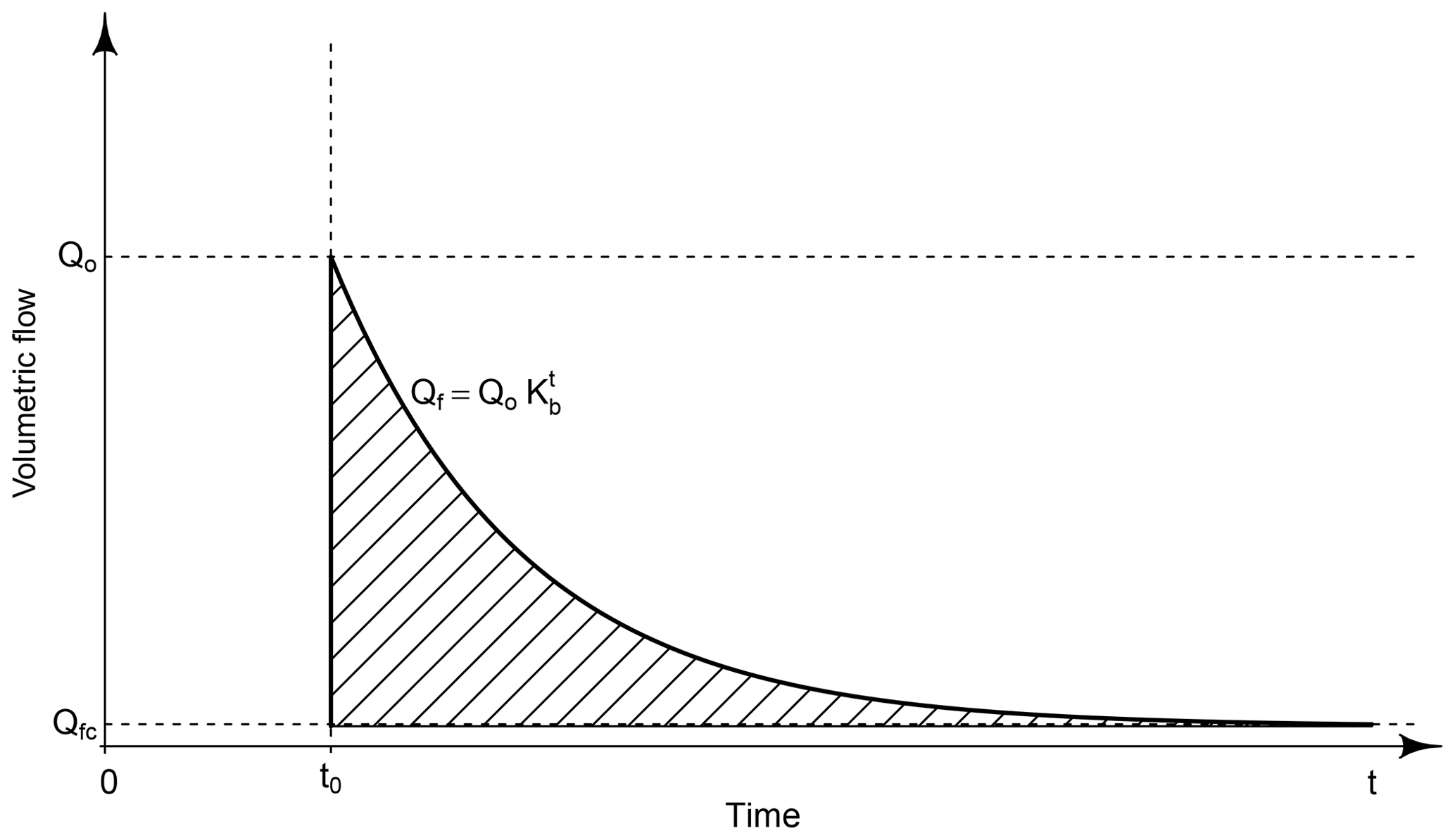
Figure 5Conceptualization of the recharge from the upslope after one precipitation at t0 using a simple linear reservoir model. The shaded area represents Eq. (44).
Therefore, if we find t from both Eqs. (43) and (44), we can set
which, solving for Qo yields
where Qfc can be found by setting θ to field capacity in Eqs. (38) and (40). Thus,
2.2.7 Evapotranspiration
The actual evapotranspiration, (mm d−1), is computed following the original formulation of Davis et al. (2017) with modifications to account for the reduction in available energy, which is diverted to snow melting and sublimation, if any. It starts by defining the actual instantaneous evapotranspiration Ea (mm h−1) as the minimum between supply SW (mm h−1) and demand Dp (mm h−1) rates (Federer, 1982).
Then, the daily integration of this flux is computed using an analogous form to the daily energy flux calculation (Fig. 6) as follows:
where h (rad) is the hour angle and hi is the cross-over angle when the supply is equal to the demand.
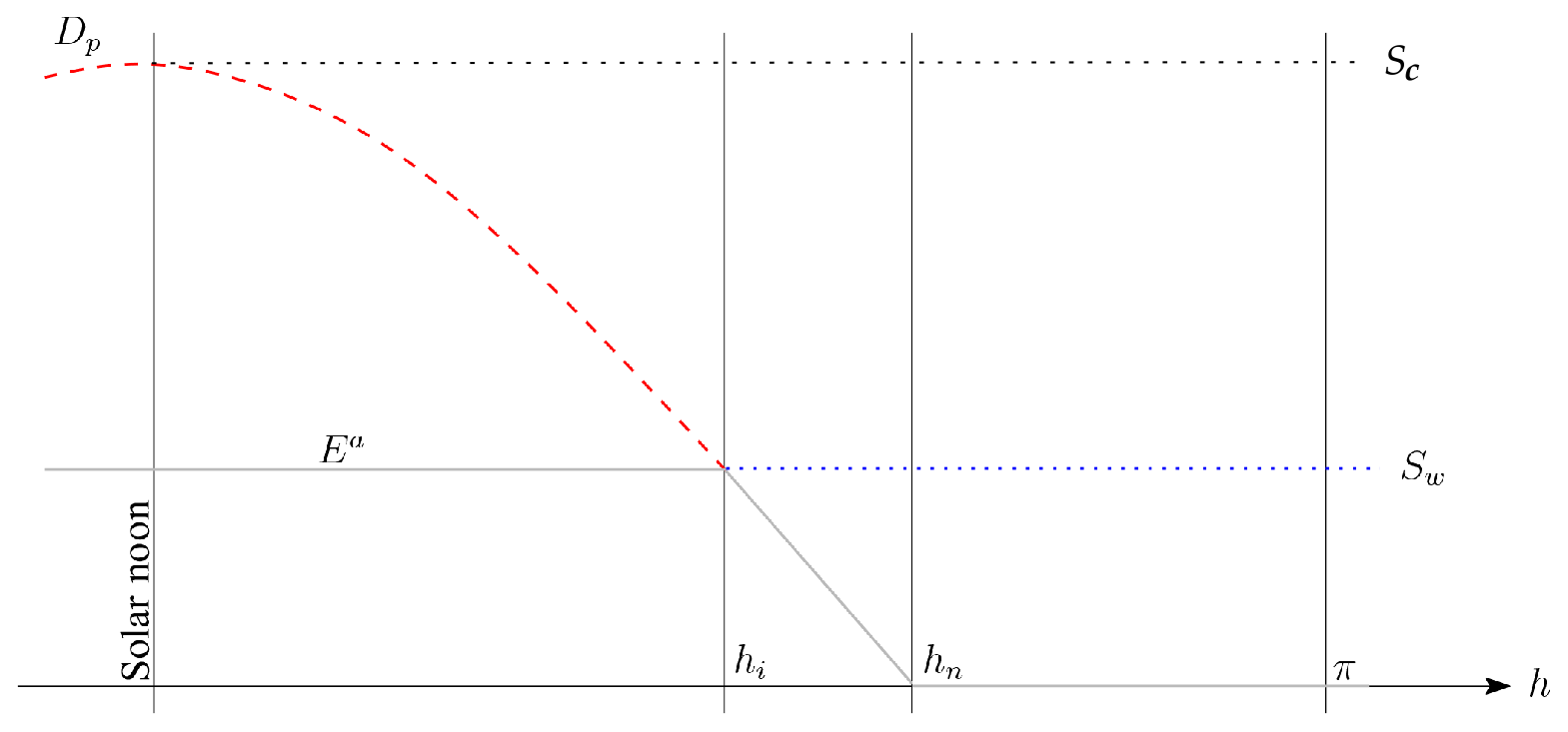
Figure 6Conceptualization of the actual instantaneous evapotranspiration flux between solar noon (i.e., h=0) and solar midnight (i.e., h=π), modified from Davis et al. (2017). The evaporative demand Dp (red dashed line) is maximum at solar noon, equivalent to the maximum supply rate, Sc. The actual supply rate SW is constant throughout the day and depends on soil moisture limitations.
The evaporative demand Dp is defined following the Priestley and Taylor (1972) formulation for potential evapotranspiration:
where IN (W m−2) is the instantaneous net radiation, and Econ (m3 J−1) is the energy-to-water conversion factor, defined following the Priestley–Taylor theory (hereafter PT), with adjustments proposed by Yang and Roderick (2019), which reproduce the feedback between the surface temperature and Ea (hence their effect on IN), thus replacing the need for a Priestley–Taylor αPT coefficient.
Here, Lv (J kg−1) is the latent heat of vaporization, ρw (kg m−3) is the water density, s (Pa K−1) is the slope of the temperature–pressure curve, γ (Pa K−1) is the psychrometric constant, and 0.24 is the constant defined by Yang and Roderick (2019). Equations for temperature and pressure dependencies to calculate ρw and γ were used, while only temperature-dependent equations were used for s and Lv (Davis et al., 2017).
The stress factor controlling the evaporative supply rate SW was conceptualized as a piecewise linear function, where we assumed the stress follows the depletion of the water content in the plant-available water region (Fig. 7).
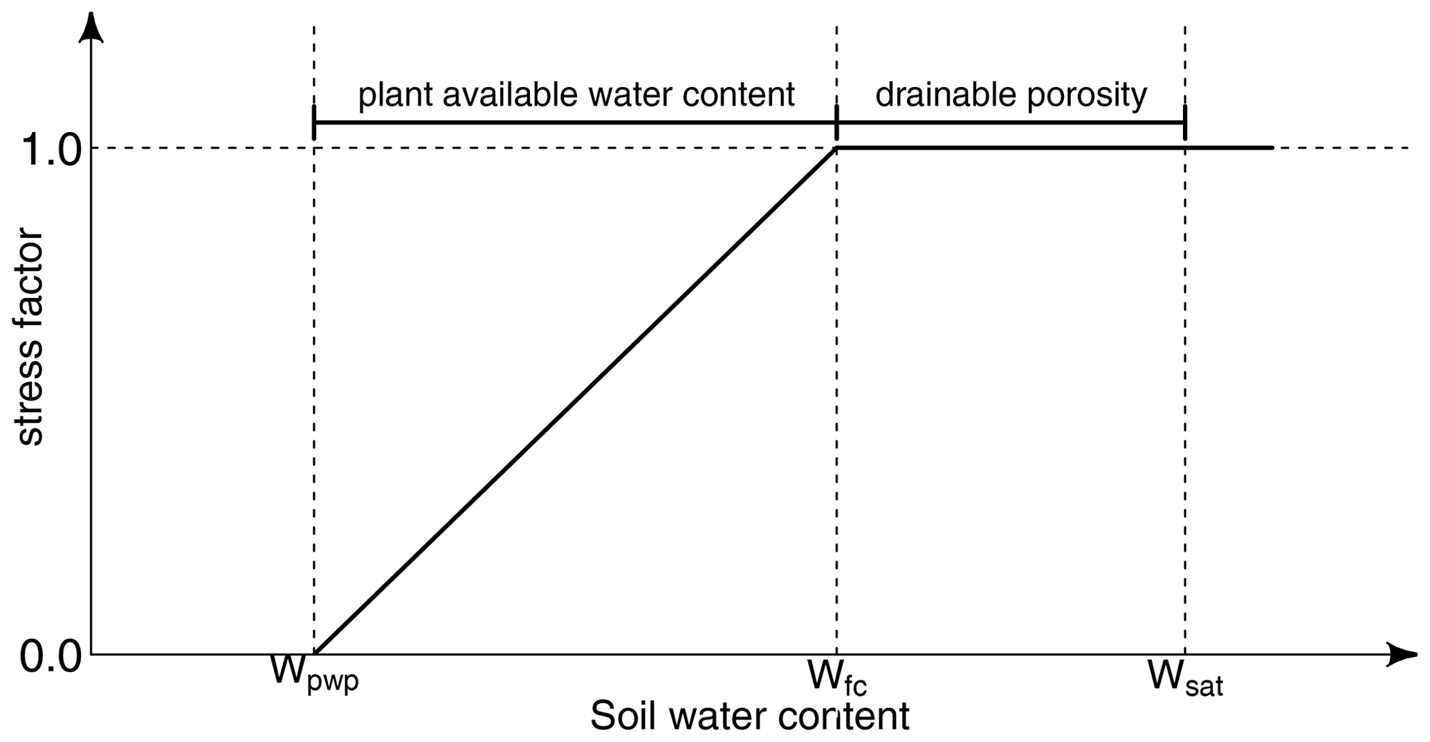
Therefore, SW is defined as
where Sc (mm h−1) is the maximum evaporative supply rate, and Wn−1 is the previous-day soil water content.
Here, Davis et al. (2017) adopt Sc as a constant, following Federer (1982); however, Federer (1982) points out that this value should change according to morphological traits of the vegetation (i.e., root density and depth).
Therefore, since , and under well-watered conditions SW=Sc, Sc with a value higher than the maximum Dp (at solar noon) will not affect the resultant Ea.
Thus, to estimate Sc so it applies for non-vegetated areas as well, the supply rate is approximated as the maximum rate of evaporation as follows:
where, to simplify the notation, rx (mm m2 W−1 h−1) is equal to 3.6×10⁶ Econ.
The upper limit of Eq. (52) is the water content at field capacity Wfc (mm), which was defined as the amount of water held after the drainage ceased (Kramer and Boyer, 1995). This was calculated by setting the total water potential to equilibrium, following Remson and Randolph (1962):
where the matric potential ψm was calculated following Saxton and Rawls (2006):
with
where θ33 is the volumetric water content at 33 kPa (usually assumed to be field capacity), θ1500 is the volumetric water content at 1500 kPa, and z (m) is the depth of the soil profile. Then, using the minimum between 2 m and the depth to the bedrock as a reference plane, the gravitational potential is defined as
Therefore, Wfc can be found by replacing Eqs. (55) to (57) in Eq. (54) and solving for Wn (see Appendix A for intermediate steps).
The lower limit of Eq. (52) is defined as the water content at permanent wilting point Wpwp (mm), which was computed as
In order to adopt the best option to compute soil hydrophysical properties (θ33, θ1500,θsat and Ksat) and hence the thresholds proposed, a set of the most widely used PTFs in LSMs were evaluated (Van Looy et al., 2017) and tested with a global dataset of soil physical properties which was compiled from different sources. The models, ranging in complexity, from the most simple mathematical formulations are described in Table 2.
Cosby et al. (1984)Balland et al. (2008)Saxton and RawlsTóth et al. (2015)(Zhang and Schaap, 2017)Table 2Evaluated pedotransfer functions and their use in land surface models.
* MLR, multiple linear regression; ANN, artificial neural network; RT, regression tree; LR, linear regression; NLR, nonlinear regression.
Thus, finally Eq. (49) is solved analytically as
where the intersection hour angle hi is found by setting Eq. (50) equal to Eq. (52) and solving for h:
2.2.8 Condensation
The daily dew formed by condensation Cn (mm d−1) is assumed to represent 10 % of the water equivalent (Eq. 52) of the negative net radiation (Eq. 15) (Jones, 2013). The remnant energy is assumed to be lost as convective heat. Thus,
2.2.9 Soil water content
Once inputs and outputs are calculated, the total soil water content Wn (mm) can now be calculated using a simple balance expression, with the previous-day soil water content Wn−1 as follows:
Furthermore, to calculate the water content (SWC) (mm) accumulated to any depth (z′) for further comparison with the observations, if we assume the same moisture profile from Eq. (26), it can be defined as
2.3 Initial conditions
The SPLASH algorithm assumed steady-state conditions as the initial state for the simulations, which is reached by looping n times the first year of data until the water balance is preserved.
3.1 Point-scale simulations
Point-scale simulations with the SPLASH model were run at individual sites (Figs. 8 and 10) with their entire daily time series of meteorological measurements. Due to different variables measured by the different networks of monitoring, the performance evaluation with the pooled data was done separately per network. The statistics used for the evaluation were the coefficient of determination (R2), the root mean squared error (RMSE), bias, and the slope of the regression for observations vs. simulations. To evaluate the seasonal patterns of fluxes and storages, all the results were aggregated as daily means and grouped by climate zone using the Köppen–Geiger climate classification system (Beck et al., 2018). Only direct measurements were used for the performance evaluations, while some indirect observations were estimated using the variation with previous-day observations to visualize seasonal patterns of some fluxes (e.g., Sf and Sme). To complement the analysis and interpretation of the results, simulations with the three-layer variable infiltration capacity model (VIC-3L) (Liang et al., 1996; Liang and Xie, 2001) were performed using the same inputs and in the same way as SPLASH, without local calibration.
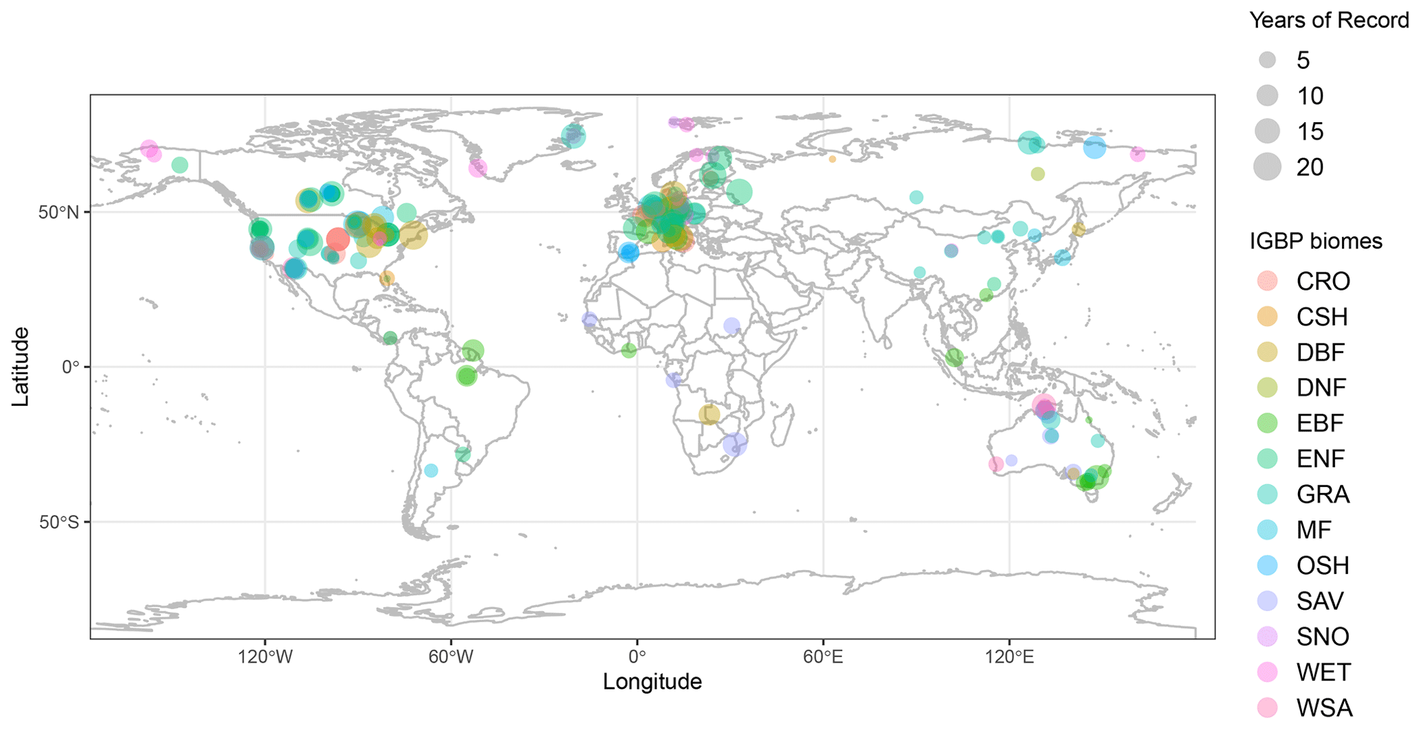
Figure 8FLUXNET stations used for the ILW parameter calibration.
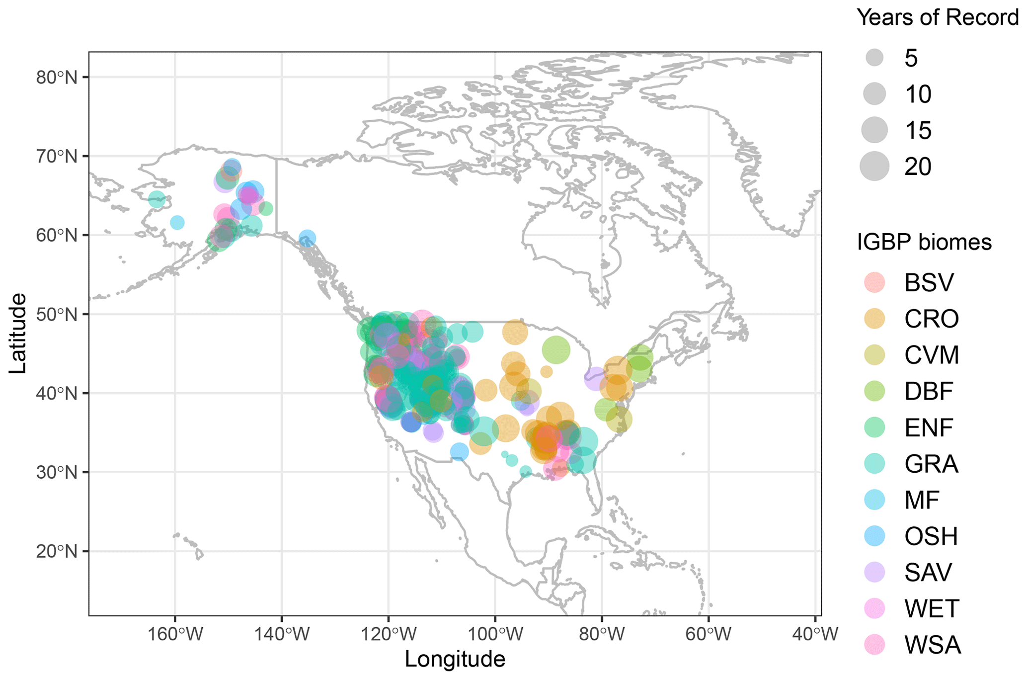
Figure 9SNOTEL stations used for albedo and snow cover analysis.
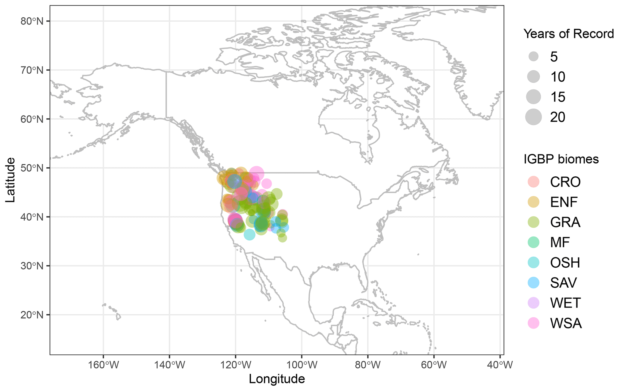
Figure 10SNOTEL soil moisture and SWE validation sites.
Vegetation properties, soil parameters, and initial soil moisture, all required by VIC-3L, were extracted at the site locations from Schaperow and Li (2020). Extra forcing data required by the VIC-3L, like wind speed and vapor pressure, not measured at the SNOwpack TELemetry (SNOTEL) sites, were extracted from the daily high-resolution GRIDMET (Abatzoglou, 2013) and DAYMET (Thornton et al., 2020) datasets, respectively. Since some quantities computed by SPLASH are not standard outputs of the VIC-3L model (e.g., and Cn), some calculations were applied to obtain comparable outputs (Appendix A3.1). To compare seasonal patterns of soil moisture a relative moisture content was calculated with the observations and results from SPLASH in the same way as the VIC output:
where Wsat is the water content (mm) at saturation. Wn and Wpwp are as defined in Sect. 2.2.7.
3.2 Spatially distributed simulations
Spatially distributed simulations were performed to visualize major spatial patterns of the fluxes and storages, test the computational performance of the model at different resolutions, and evaluate how the global parameters and assumptions of the model hold.
Global simulations were run at a resolution of 5 km, regional simulations (e.g., North America) at a resolution of 1 km, and micro-catchments at a resolution of 90 m. Since the model lacks a routing algorithm, to test the runoff–lateral flow simulations against streamflow observations, yearly aggregated quantities were used.
VIC spatially distributed simulations of runoff across the US were obtained from Kao et al. (2022). These simulations, conducted independently, employed VIC calibrated with historical hydrological data and were exclusively used for evaluating streamflow against SPLASH simulations run with identical inputs (i.e., DAYMET, Thornton et al., 2018).
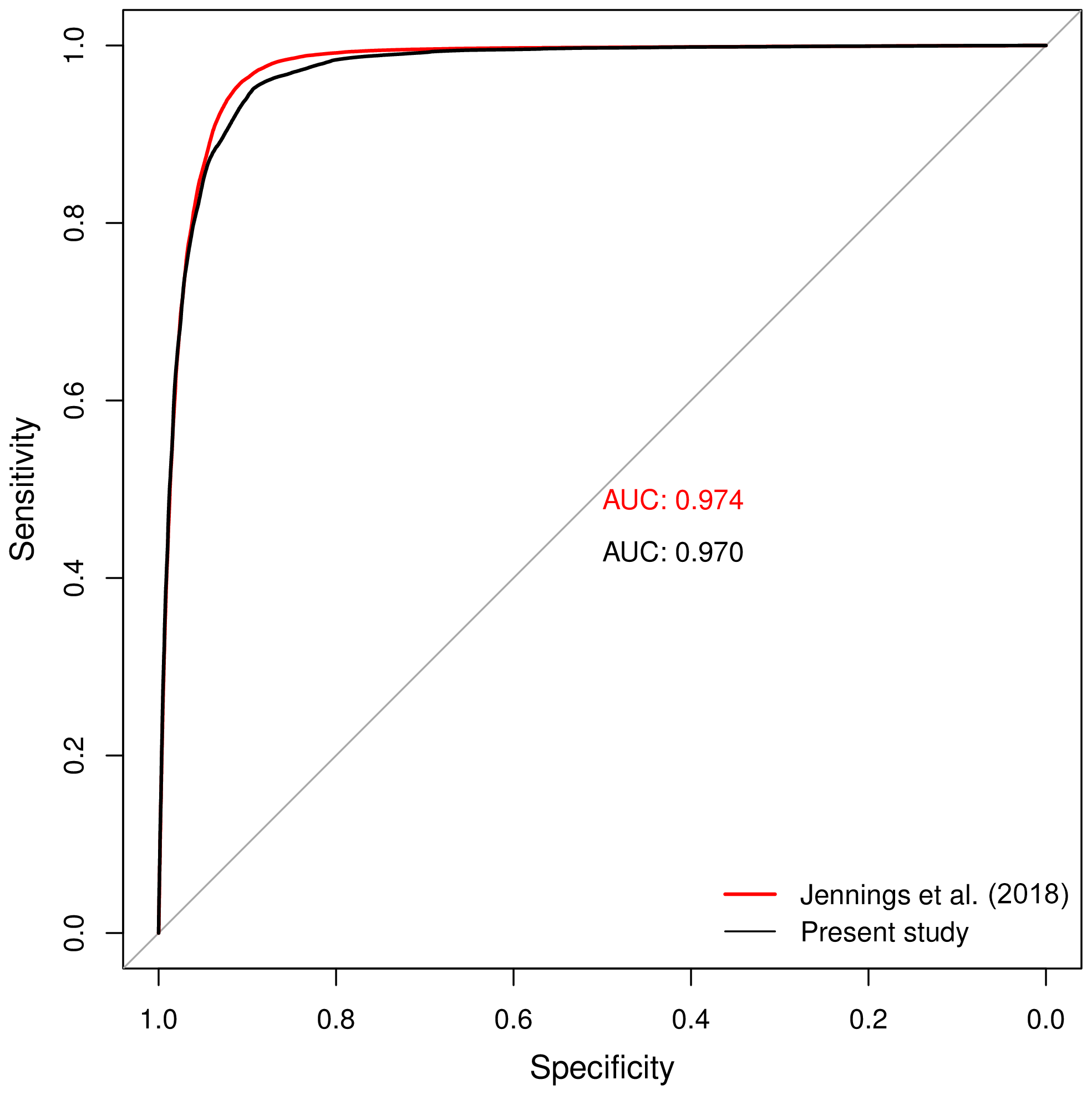
Parameters from the selected equations (pedotransfer functions) were optimized using the Nash–Sutcliffe (NSE) coefficient, which relates the variance of the residuals to the variance of the data as the objective function (Nash and Sutcliffe, 1970; Gupta and Kling, 2011). Here, an NSE closer to 1.0 expresses ideal estimates. The probabilistic model for snowfall occurrence was fitted using a binomial family generalized linear model (GLM), while the albedo-related functions were fitted using nonlinear least squares. To assess the accuracy of the snowfall probability estimation, the receiver operating characteristic (ROC) curve was used, which plots the true positive rate (specificity) against the false positive rate (sensitivity) using a probability of 0.5 as a threshold. Here the area under the curve (AUC) closer to 1.0 expresses a better overall prediction (Fawcett, 2006).
5.1 Eddy covariance towers
Data from the whole FLUXNET database (Pastorello et al., 2020), comprising 212 stations distributed around the world (Fig. 8), were used to update the empirical functions to compute net longwave radiation, superseding the equations formulated by Monteith and Unsworth (1990) and Linacre (1968) used in the first version of SPLASH.
All the data were aggregated to daily means, while the originally reported latent heat flux was transformed to its equivalent in water flux density (mm d−1) by using the heat of vaporization corrected for field conditions.
To test the validity of the theorized daily cycles and cross-over angles, positive values of net radiation were subsetted and aggregated daily, which in theory should be equivalent to Eq. (14). A simple threshold for measured albedo of 0.3 was used to identify snow presence; then, latent heat measurements when snow was present were excluded from the estimations of daily evapotranspiration and condensation, trying to prevent the latent heat used in melting, refreeze, and sublimation from introducing error into the evaluations.
5.2 Meteorological and hydrometric stations
To estimate the parameters used in the snow cover and albedo functions, 315 stations reporting snow-water equivalent or snow depth from the SNOwpack TELemetry (SNOTEL) network (Serreze et al., 1999), managed by the US Natural Resources Conservation (NCAR) service, were used together with remote sensing data (Fig. 9); most of these stations also report solar radiation, precipitation, air temperature, and volumetric soil moisture at different depths.
To evaluate the model, we subset sites in mountain regions with joint measurements of snow, soil physical properties (i.e., texture, bulk density, and SOM), and soil moisture deeper than 30 cm, resulting in 127 sites (Table A5). Data from the DAYMET database (Thornton et al., 2018) were used whenever the solar radiation was not reported (Fig. 10).
To fit the binary logistic regression used to estimate the probability of snowfall occurrence p(snow), the dataset described by Jennings et al. (2018) was used, which comprises 11 924 stations distributed over the Northern Hemisphere, adding a total of 17 810 805 binary observations of snowfall (Fig. 11).

Figure 11Stations providing snowfall observations from the Jennings et al. (2018) dataset.
To test the model capabilities predicting streamflow, with its improvements accounting for slope, small watersheds with areas between 5 and 2000 km2 located in mountain regions of Canada and the USA were selected from the global GSIM database (Do et al., 2018) due to the quality of the available forcing data over these regions. The GSIM database provides curated streamflow data from multiple sources and geographic watershed boundaries (Fig. 12). Only watersheds with natural cover higher than 90 % and streamflow data covering at least 10 years since 1980 were subset (Table A6), resulting in 15 963 station years. Here, the separation of surface runoff and baseflow was done following the method described by Ladson et al. (2013).
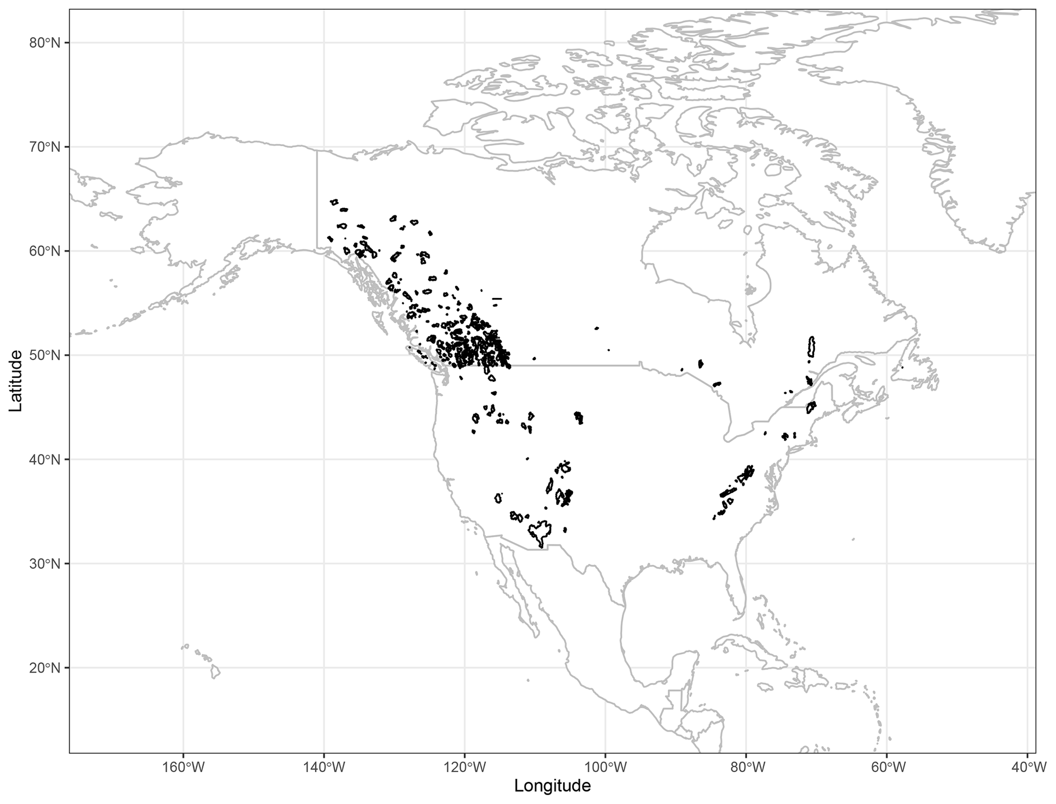
Figure 12GSIM watersheds for streamflow validation.
To evaluate the spatial patterns produced by the model with long-term data, hydrometeorological and soil moisture measurements from the Rietholzbach Research Catchment were used. These datasets are publicly available and described by Seneviratne et al. (2012) and Hirschi et al. (2017). To test the model in regions where the rainfall and runoff response is mainly dominated by subsurface flow (Crespo et al., 2011; Correa et al., 2020), hydrometeorological data from the tropical Andes, compiled by Ochoa-Tocachi et al. (2018), were used.
5.3 Soil physical properties and terrain
To calibrate the pedotransfer functions which compute field capacity (θ33) and wilting point (θ1500) a dataset containing data on water retention, texture, organic matter content (SOM), and bulk density was compiled from the US Natural Resources Conservation service through the “soilDB” R package (Skovlin and Roecker, 2018) and the “Wosis” databases (Batjes et al., 2020). Both databases have global coverage and resulted in a total of 68 567 usable samples (at least one of the response variables (θfc or θwp) and all the predictors) out of 324 380 (Fig. 13).
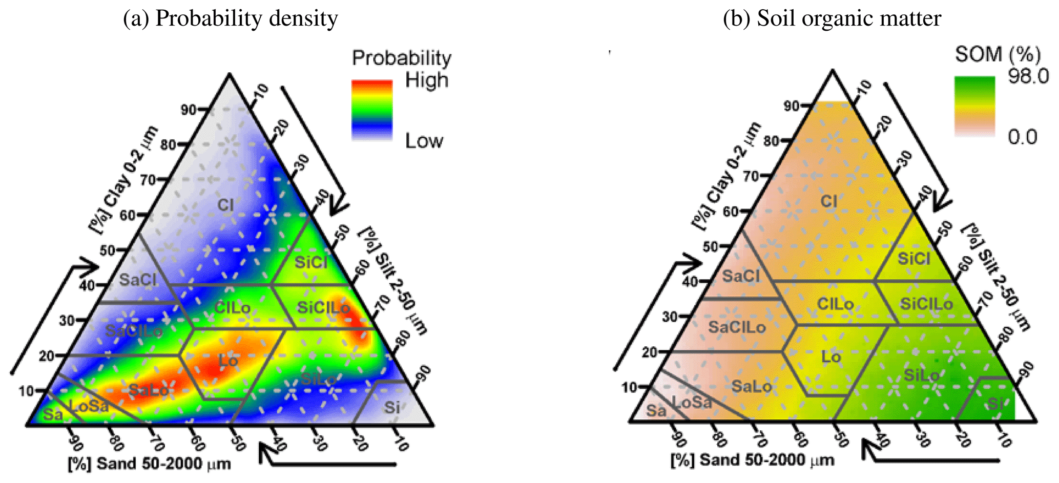
Figure 13θfc and θwp measurements used to calibrate the pedotransfer functions. (a) Probability density of the soil samples according to their textural classes. (b) Average soil organic matter content of the samples per textural class.
To optimize the functions to estimate soil moisture at saturation (θsat) and saturated hydraulic conductivity (Ksat) data were gathered from the HYBRAS (Ottoni et al., 2018), SWIG (Rahmati et al., 2018), UNSODA (Leij et al., 1996), and University of Florida (IFAS, 2007) datasets for a total of 9346 usable samples out of 15 160 (Fig. 14).
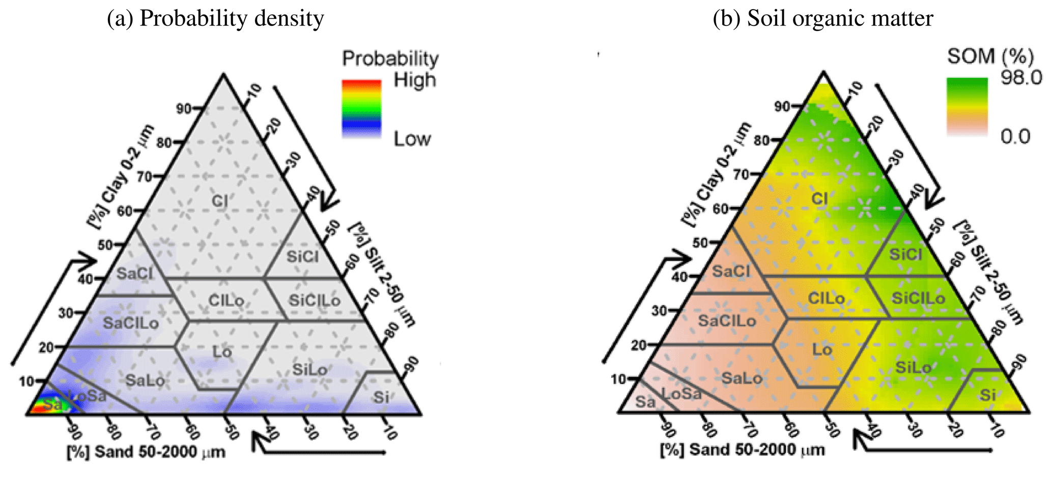
Figure 14Ksat and θsat measurements used to calibrate the pedotransfer functions. (a) Probability density of the samples according to their textural classes. (b) Average soil organic matter content of the samples per textural class.
To test the model for the EC sites, abovementioned soil physical properties were retrieved from the SoilGrids.org (https://soilgrids.org/, last access: 26 January 2021) dataset (Hengl et al., 2017), while the “soilDB” R package (Skovlin and Roecker, 2018) was used to retrieve soil data at SNOTEL sites.
Slope, slope orientation (aspect), and upslope area were computed using the TauDEM software (Tarboton, 2016) from the global SRTM digital elevation model resampled to 250 m (Jarvis et al., 2008).
5.4 Remote sensing
To fit the functions that calculate the snow cover fraction and the snow cover effect on the albedo, data from the MODIS MOD10A1 500m daily product (Hall et al., 2016) were compared against 15 years (2001–2015) of daily data from the 315 SNOTEL stations described previously in this section (Fig. 9).
Information on the biome classification, used to interpret the data, was gathered from the simple typology defined by the International Geosphere–Biosphere Programme (IGBP), available as a MODIS product (MOD12Q1) (Friedl et al., 2019).
To assess the spatial patterns of evapotranspiration in selected small watersheds, the SEBAL algorithm (Bastiaanssen et al., 1998a, b), implemented in Google Earth Engine (GEE) by Laipelt et al. (2021), was used with Landsat 5 atmospherically corrected surface reflectances from 1994–2007 and Landsat 8 from 2014.
To propose a reasonable assumption for the duration of a precipitation event, the global hourly precipitation GsMAP dataset was used. This dataset has 0.1° resolution and was built using retrievals from NASA's satellite constellation, including infrared, microwave, and radar sensors (20 sensors), merged and corrected with NOAA’s ground stations (Mega et al., 2014; Yamamoto and Shige, 2015). Since the gauge count is also available within the dataset, only pixels with three or more gauges were used to extract and analyze the hourly data using GEE.
5.5 Spatially distributed forcing
For the global simulations at 5 km of resolution, monthly precipitation data from Beck et al. (2019) were resampled and subset to 2010–2016, and air temperature was obtained from the Terraclim dataset (Abatzoglou et al., 2018), together with the solar radiation produced by Ryu et al. (2018), which uses MODIS atmospheric and albedo retrievals as some of the inputs.
For regional simulations (e.g., North America), 1 km resolution temperature and precipitation from CHELSA (Karger et al., 2017) were used, while the solar radiation from Ryu et al. (2018) was downscaled using the theoretical effects of terrain described in Sect. 2.1.1. Elevation datasets at 1 and 5 km resolution used in the respective runs were obtained from Amatulli et al. (2018). While the soil data were resampled from the global 250 m SoilGrids dataset (Hengl et al., 2017) (sand, clay, organic matter, coarse fraction, and bulk density), the soil depth and thickness were averaged between SoilGrids and the Pelletier et al. (2016) datasets.
6.1 Fitting and optimization results
6.1.1 Net longwave radiation functions
Quadratic equations were the best fit for both incoming and outgoing longwave radiation during clear-sky conditions, noticeably improving the predictions for temperatures below 0 °C, particularly useful for regions at high elevations (Fig. 15a and b). The net longwave equation, resulting from algebraically subtracting LWIN−LWOUT, showed a very small quadratic coefficient, which was neglected to adopt a simpler linear equation (Fig. 15c).
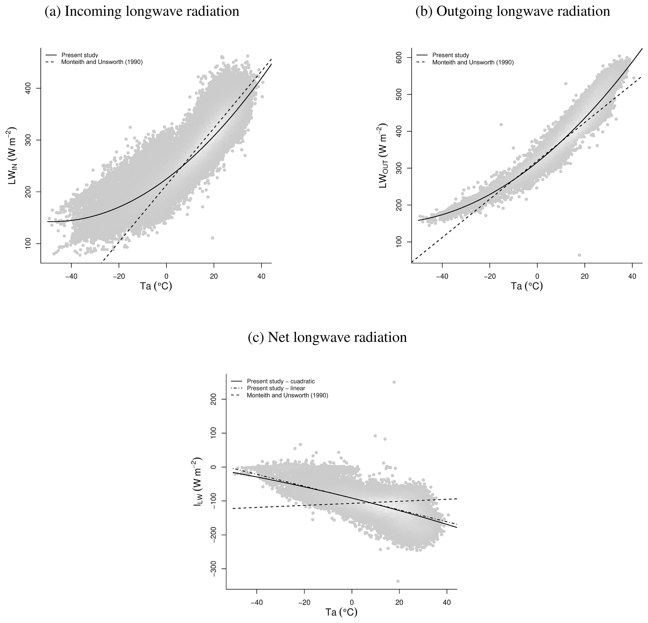
Figure 15Clear-sky longwave radiation as a function of air temperature. (a) Clear-sky incoming longwave radiation. (b) Clear-sky outgoing longwave radiation. (c) Clear-sky net longwave radiation.
6.1.2 Snowfall probability
The performance of the snowfall occurrence calculation resulted in an AUC of 0.97 (Fig. 16), which considering a maximum value of 1.0 suggests that this method is highly accurate.
6.1.3 Snow cover fraction and snow albedo correction
The simple hyperbolic function used to describe the response of the snow cover fraction to the size of the snowpack suggests that the inflection starts when the SWE reaches 140 mm, and most of the variation in snow cover (up to 80 %) happens in the first 1000 mm of SWE. Moreover, the standard deviations of SWE aggregated by biomes show that in the sampled period values higher than 1000 mm are uncommon (Fig. 17a).
The snow aging function suggests that a reduction of about 50 % of the albedo can happen in the first 10 d without new snow falling and the lowest albedo can reach 0.4 (Fig. 17b).
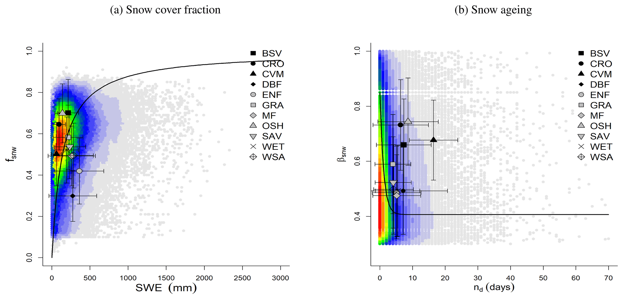
Figure 17Ground-based observations of snow against satellite retrievals. The color scale represents the plotted point density, where blue indicates lower densities and red indicates higher densities. (a) Daily snow cover fraction from MODIS (fsnw) vs. daily SNOTEL SWE. The black line shows the optimized Eq. (27). (b) MODIS albedo (βsnw) when the snow cover exceeds 70 % vs. days without fresh snowfall (nd) from the daily SNOTEL SWE. The black line shows the optimized Eq. (26).
6.1.4 Pedotransfer functions
From the models tested (Table 2), the nonlinear equations from Balland et al. (2008), which were fit to the largest dataset, outperformed the other models. Further optimization of these equations (Eqs. A25a, A25b, A25c) using the full dataset employed for this evaluation yielded a slight improvement of around 10 % for field capacity (θ33) and saturation (θsat) (Fig. 20). The new parameters are detailed in Table A1.
Here, θ1500 is wilting point (water held at 1500 kPa), θ33 is field capacity (water held at 33 kPa), θsat is saturation, Ksat is the saturated hydraulic conductivity, and, SAND, CLAY, and SOM refer to sand, clay, and organic matter contents (%). a, b, and c are constants with the subscripts referring to wilting point, field capacity, or hydraulic saturated conductivity, respectively, ρb is the bulk density, and ρp is the particle density, calculated as follows (Balland et al., 2008):
Ksat estimated by the Saxton and Rawls (2006) PTF was the best-performing model; however, it leads to unrealistic values when the drainable porosity (θsat−θ33) is relatively high. Thus a simple saturating curve was adopted here, which yields similar estimations to Saxton and Rawls (2006) at the lower end of the drainable porosity but flattens at a fitted Ksat maximum of 623 mm h−1.
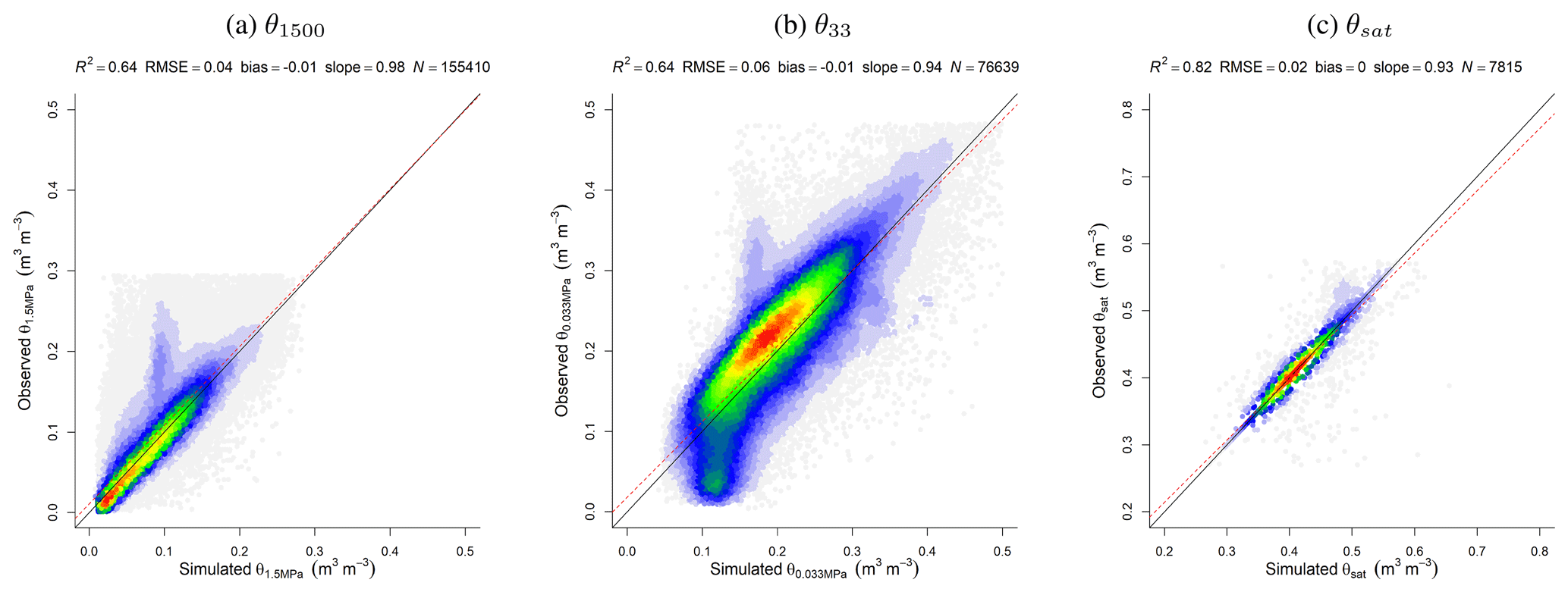
Figure 18Correlation of observed and simulated values of soil hydrophysical properties. The color scale represents the plotted point density, where blue indicates lower densities and red indicates higher densities. (a) Permanent wilting point (θ1500). (b) Field capacity (θ33). (c) Soil porosity or saturation point (θsat).
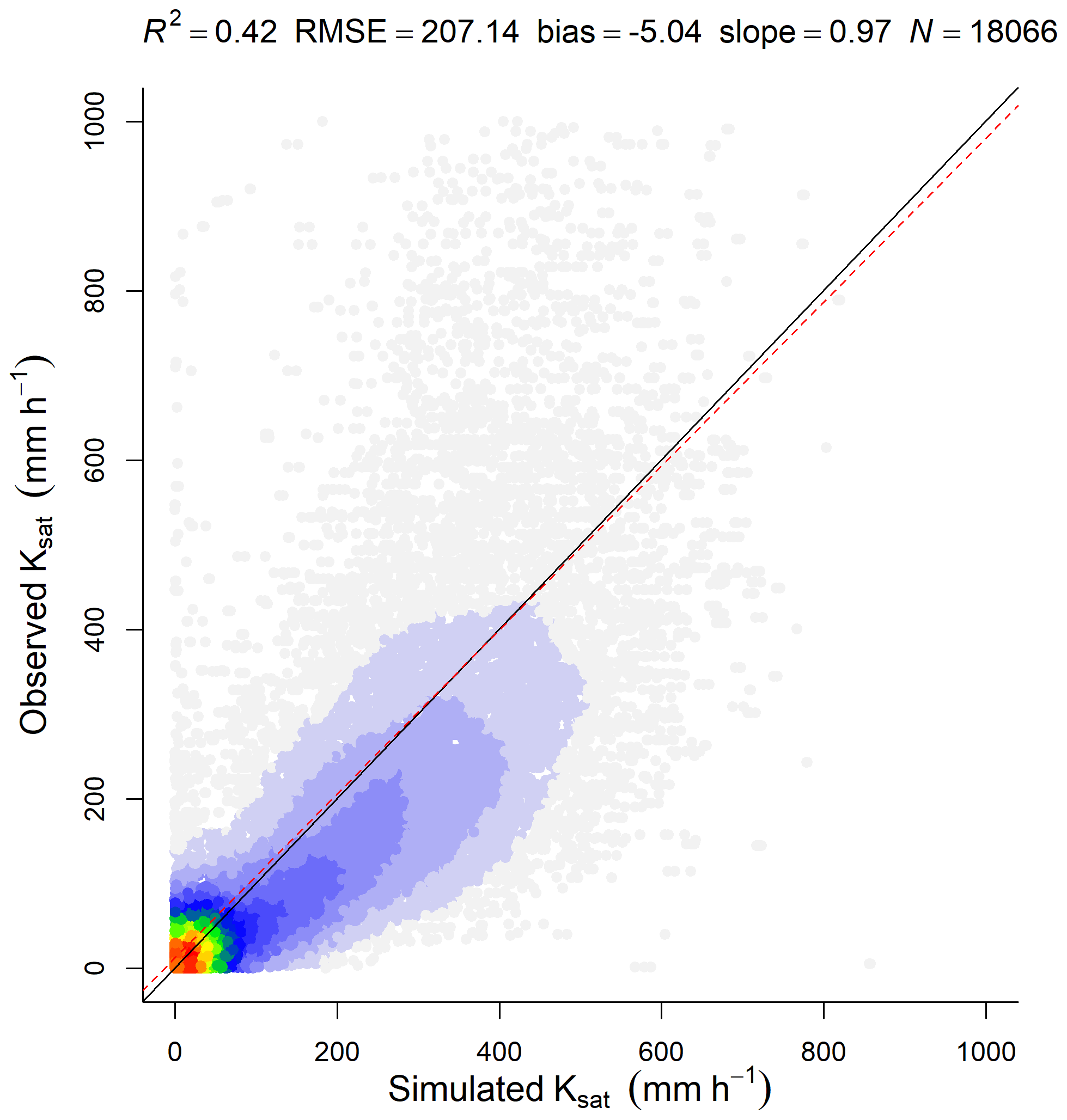
Figure 19Correlation of observed and simulated values of saturated hydraulic conductivity Ksat. The color scale represents the plotted point density, where blue indicates lower densities and red indicates higher densities.
6.2 Fluxes
6.2.1 Net longwave radiation
The evaluation of ILW shows the values clustering around −100 and 0 W m2; nonetheless, the simple linear model was able to explain 70 % of the variance with a very low bias (−0.11) (Fig. 20).
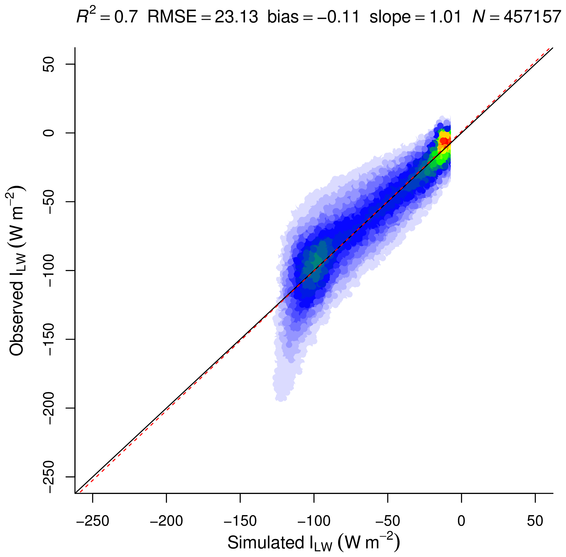
Figure 20Correlation of observed and simulated values of ILW, with data from all the sites pooled. The color scale represents the plotted point density, where blue indicates lower densities and red indicates higher densities.
6.2.2 Daytime net radiation
The daytime net radiation, or positive net radiation, was compared against 87 EC sites distributed over mountain regions covering several biomes. The comparison, using all the data pooled at daily resolution shows, that the model is able to explain more than 70 % of the observations' variance with a very small bias (Fig. 21). The evaluation also shows that the highest overestimation happens in ecosystems with sparse vegetation (BSV biome).
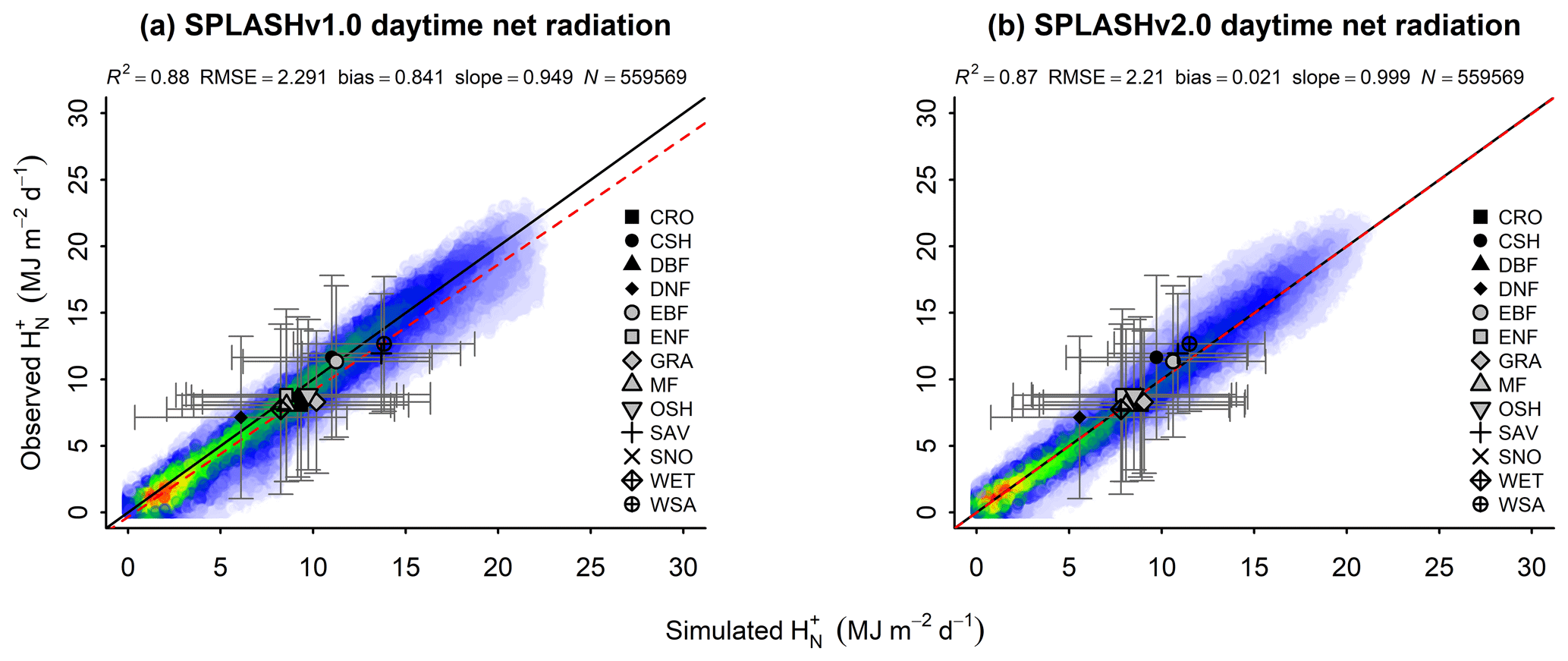
Figure 21Correlation of observed and simulated values of with data from all the sites pooled. The color scale represents the plotted point density, where blue indicates lower densities and red indicates higher densities. (a) Simulations with SPLASH v1.0. (b) Simulations with SPLASH v2.0.
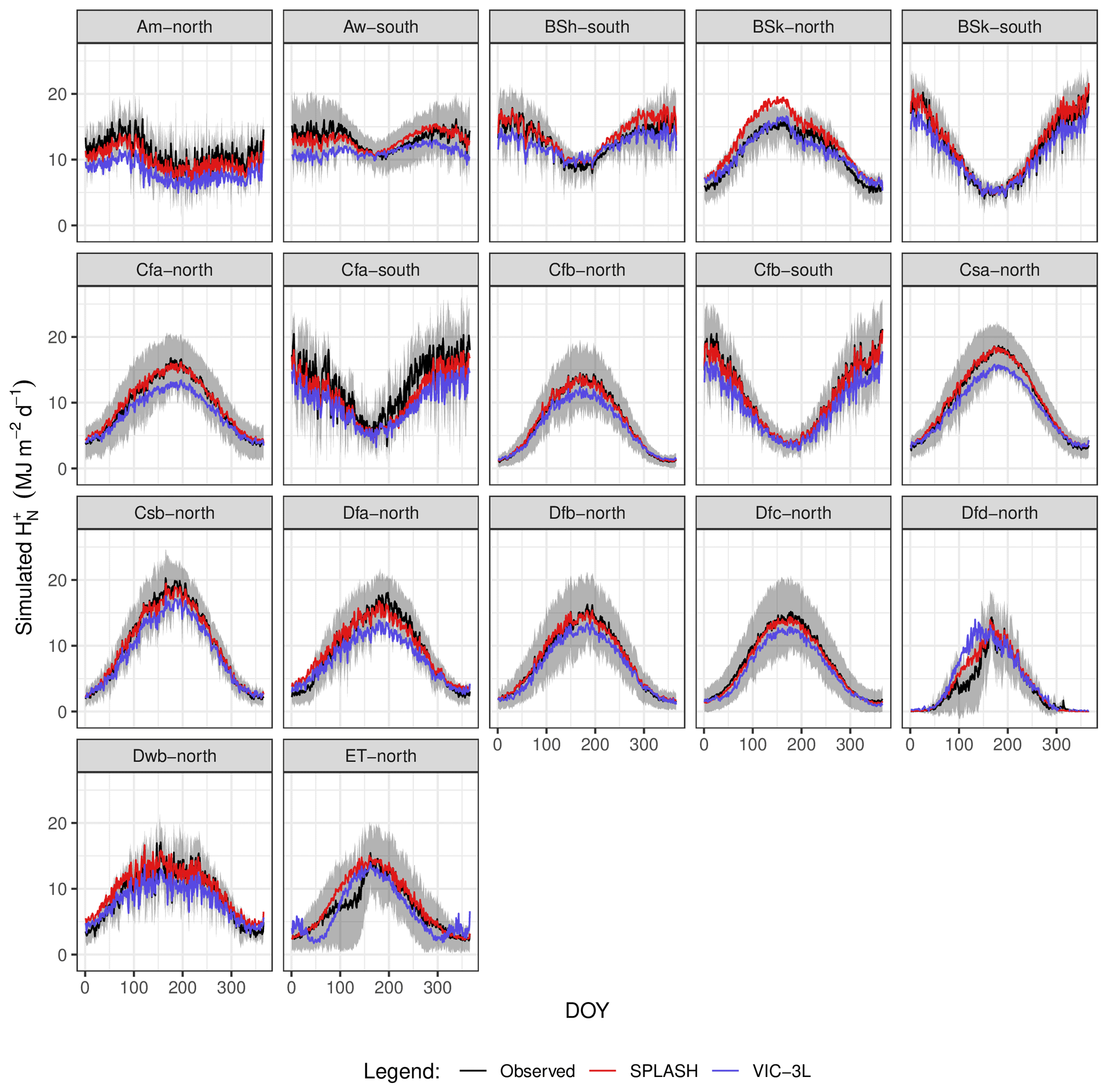
The seasonal patterns of averaged by climate zone show a classic bell-shaped curve, peaking during the summer months, with greater deviations from the mean appearing in climate zones with no dry season (Cfb, Dfc). SPLASH simulations reproduce the observations more closely than the VIC results in most of the climate zones, noticeably outperforming VIC in climate zones with dry summers (Csa, Csb). SPLASH overestimation happens primarily in cold deserts during summer months (BWk), while underestimation is noticeable in temperate zones with no dry season (Cfa) and in the hot steppe (BSh), both during summer months (Fig. 22).
6.2.3 Evapotranspiration
The performance evaluation of using the data from all the EC stations shows the model reproducing 50 % of the variance of daily observations with a small bias and the slope of the regression of observations simulations equal to 0.072. The standard deviation of the data aggregated by biome, in the observation axis, shows that at a daily time step is highly variable, and there is no clear difference between woody and herbaceous ecosystems. The evaluation shows a greater underestimation for evergreen broadleaf forests (EBF), while the greater overestimation happens in deciduous broadleaf forests (DBF). Furthermore, the lowest is shown by ecosystems with sparse vegetation (OSH) and the highest by EBF (Fig. 23).
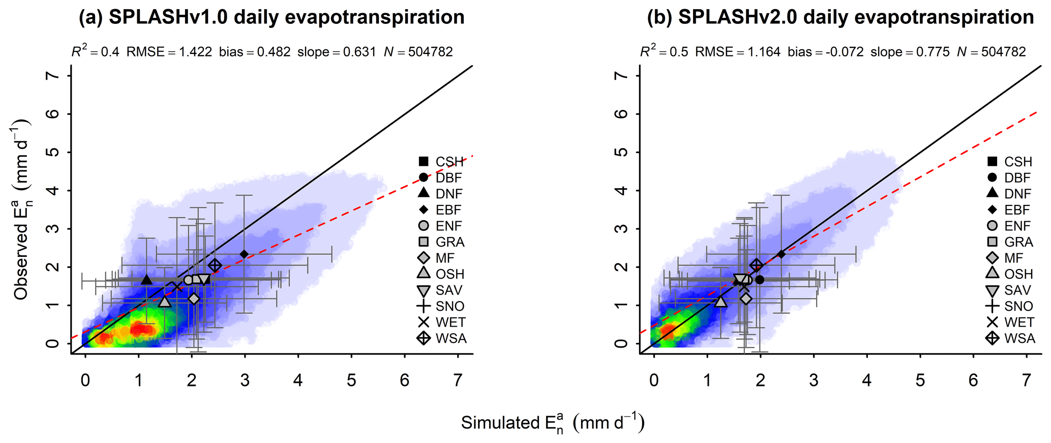
Figure 23Correlation of observed and simulated values of with data from all the sites pooled. The color scale represents the plotted point density, where blue indicates lower densities and red indicates higher densities. (a) Simulations with SPLASH v1.0. (b) Simulations with SPLASH v2.0.
The seasonal patterns of broadly follow the pattern of in zones with no water limitations (Cf* and Cf* types), and the polar tundra exhibits similar patterns but with a higher difference between summer and winter months. Arid zones (BS* and BW* types) show a very different pattern compared to . SPLASH simulations correctly reproduced most of the seasonal patterns and for certain climate zones (BSk, Csb, Dsc) outperformed VIC simulations. Although SPLASH captures the overall seasonal patterns, it overestimates at Dsc sites, while, similarly to the VIC results, it underestimates in the polar tundra (ET) and at the Cfb sites in the Southern Hemisphere (Fig. 24).
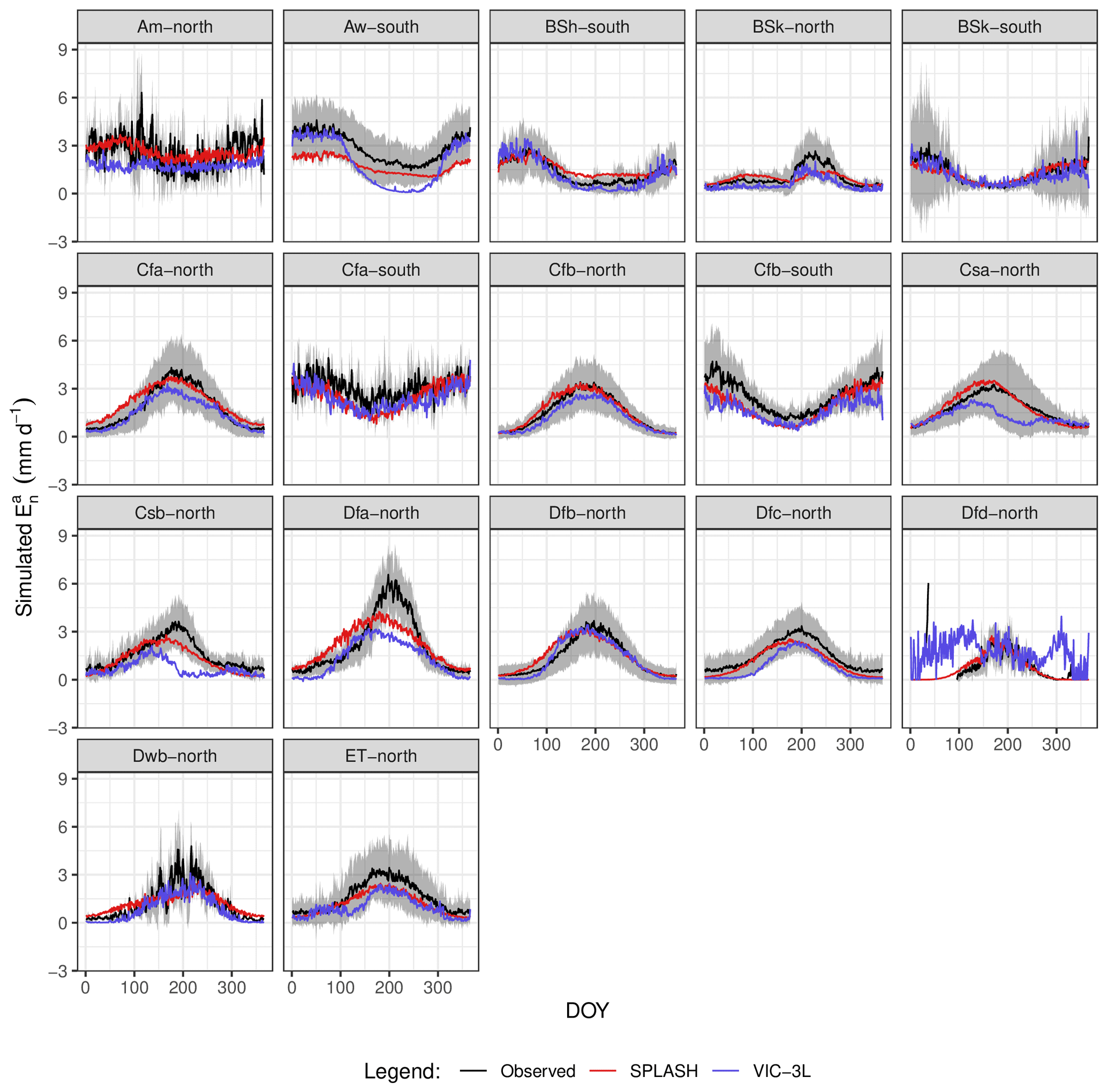
Figure 24Mean seasonal cycle of per climate zone. The gray areas show 1 SD from the observed mean. Climate zones are described in Table A3.
At a global scale, SPLASH produces major spatial patterns that roughly follow the distribution of the Köppen–Geiger climate zones. In northern latitudes it overestimates during summer months; nonetheless, it outperforms VIC-3L, which produces high values during winter (Fig. 25).
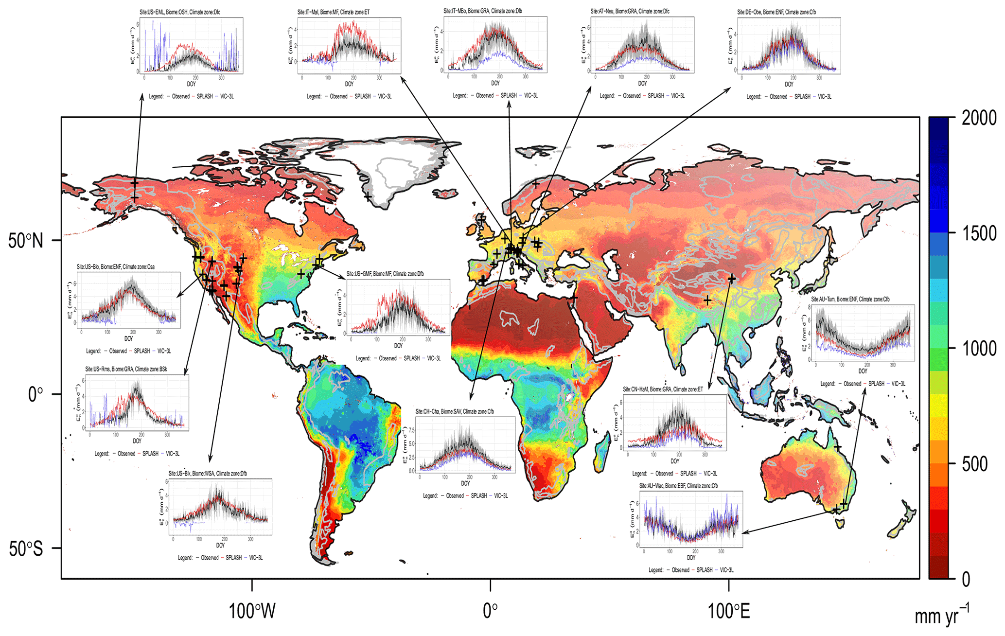
Figure 25Spatial patterns of mean annual Ea for the period 2010–2016 at 5 km resolution along with site simulation examples from the mountains. Inset plots show seasonal cycles where observations are in black, SPLASH v2.0 simulations are in red, and VIC-3L simulations are in blue. The gray areas show 1 SD from the observed mean.
The simulations, with the long-term data from Rietholzbach, exhibit good overall agreement with the lysimeter-based observations (Fig. 26c). However, a minor but systematic overestimation happens during the spring months. Here, the spatial patterns produced by SPLASH show higher magnitudes on south-facing slopes and at the valley bottom close to the outlet, coinciding with the area where a small forest is present (Seneviratne et al., 2012) (Fig. 26c). These patterns contrast with the spatially distributed LE, calculated from Landsat 5 retrievals, which shows a more uniform LE, except for a few forest patches, where LE spikes (Fig. 26d). Both datasets barely agree over the small forest at the valley bottom.
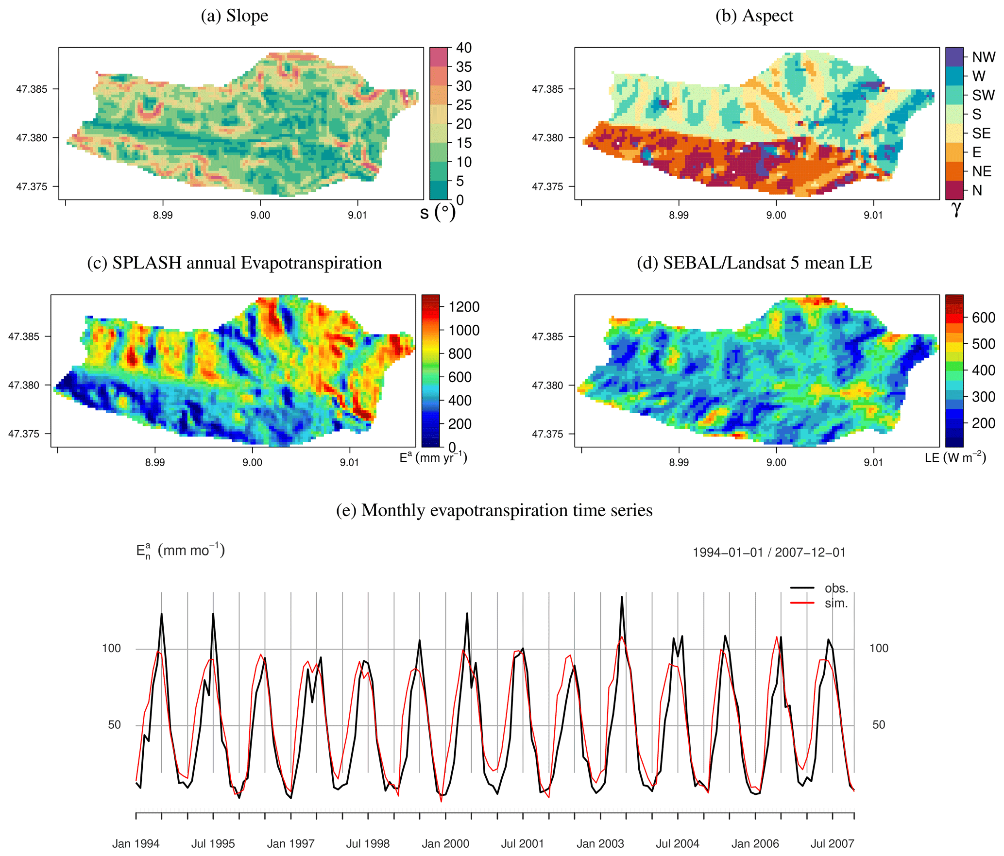
Figure 26Spatial and temporal patterns of evapotranspiration in a small wet temperate watershed in Rietholzbach, Switzerland. (a) Slope in degrees. (b) Slope orientation; N stands for north, S for south, and so on. (c) Mean annual simulated evapotranspiration 1994–2007. (d) Mean instantaneous LE from L5's clear-sky pixels during 1994–2007. (e) Time series of monthly evapotranspiration, as well as simulated and lysimeter-based observations.
In the tropical watershed, the spatial patterns of produced by SPLASH (Fig. 27c) show better agreement with the RS LE than in the temperate watershed, as shown by some emergent cold spots in the northern part of the watershed (Fig. 27e). Moreover, in both datasets, slopes facing the Equator show higher magnitudes compared to flat areas; however, in the SPLASH results, this difference is stronger than in the RS LE estimation.
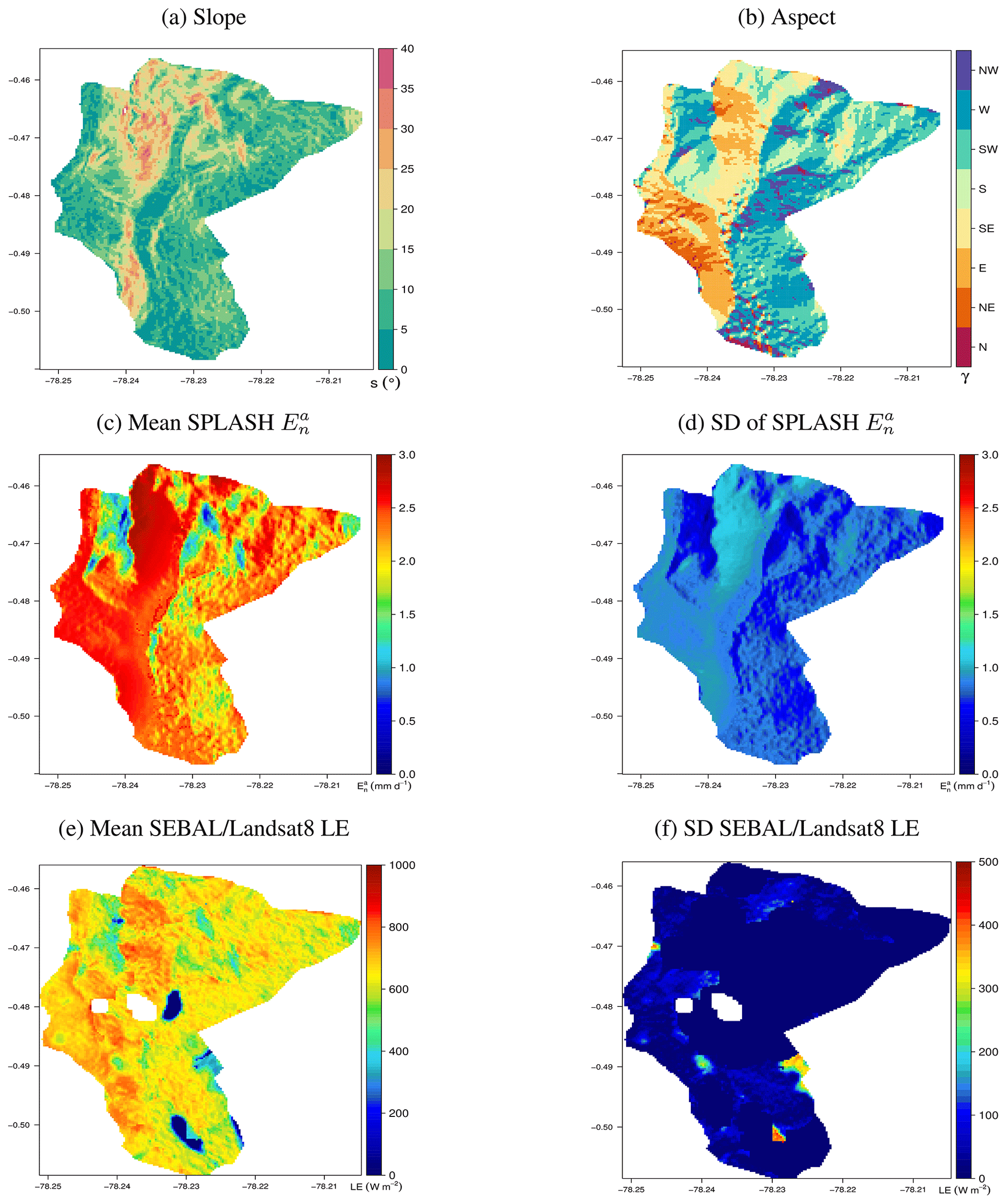
Figure 27Spatial patterns of daily evapotranspiration in a wet tropical watershed in Jatunhuayco, Ecuador. (a) Slope in degrees. (b) Slope orientation; N stands for north, S for south, and so on. (c) Mean daily evapotranspiration during 2014. (d) Standard deviation of the daily evapotranspiration during 2014. (e) Mean instantaneous LE from L8's clear-sky pixels during 2014. (f) Standard deviation of the instantaneous LE from L8's clear-sky pixels during 2014.
6.2.4 Condensation
The model showed the poorest performance simulating Cn, capturing only around 18 % of the variance, with a bias of 0.913. The slope of the regression of observations vs. simulations points to overestimations at high simulated values; however, it shows a massive improvement from version 1.0 (Fig. 28). Most of the observations seem to cluster in the 0–10 mm yr−1 range, with the greatest underestimation occurring in broadleaf evergreen forests, while Cn is overestimated in barren and sparsely vegetated ecosystems.
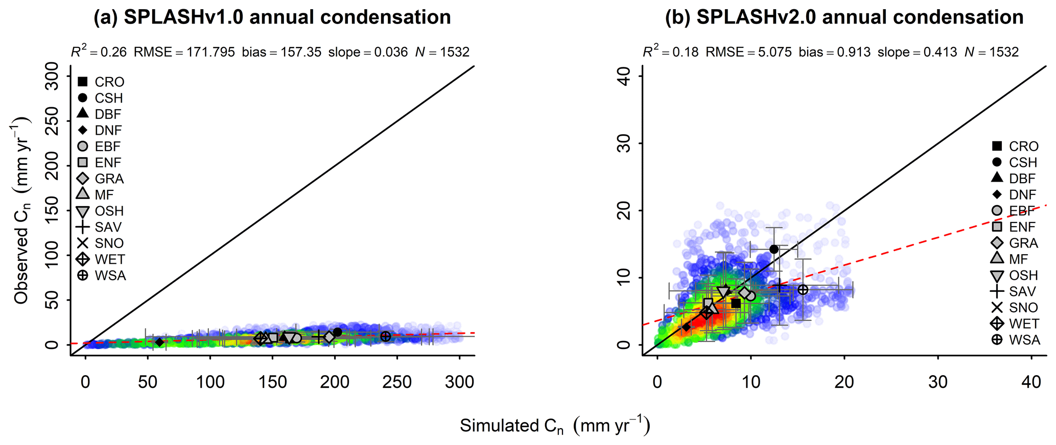
Figure 28Correlation of observed and simulated values of Cn with data from all the sites pooled. The color scale represents the plotted point density, where blue indicates lower densities and red indicates higher densities. (a) Simulations with SPLASH v1.0. (b) Simulations with SPLASH v2.0.
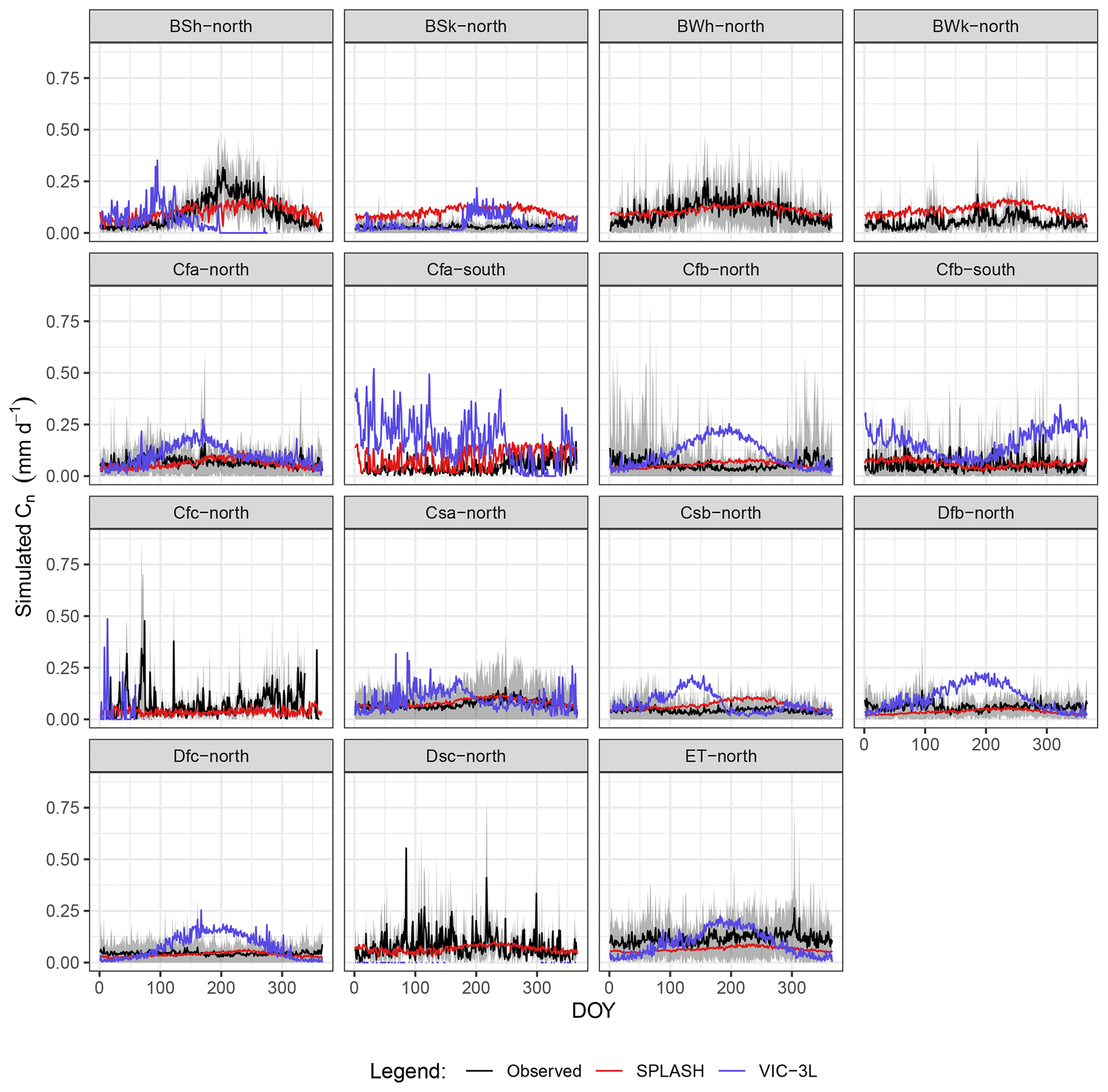
Just arid climate zones (B* types) showed seasonal patterns of Cn and potentially important magnitudes, and both dimensions are captured by SPLASH. However, the SPLASH model is still underestimating Cn in the hot steppe (BSh) and overestimating Cn in the cold steppe and desert (e.g., BSk and BWk). In some climate zones with no apparent seasonal pattern and with random peaks through the year (e.g., Cfc and Dsc) the SPLASH model shows a smother prediction, underestimating all the peaks. Compared to the VIC simulations, the SPLASH model seems to reproduce the general patterns more reasonably (Fig. 29).
6.2.5 Snowfall
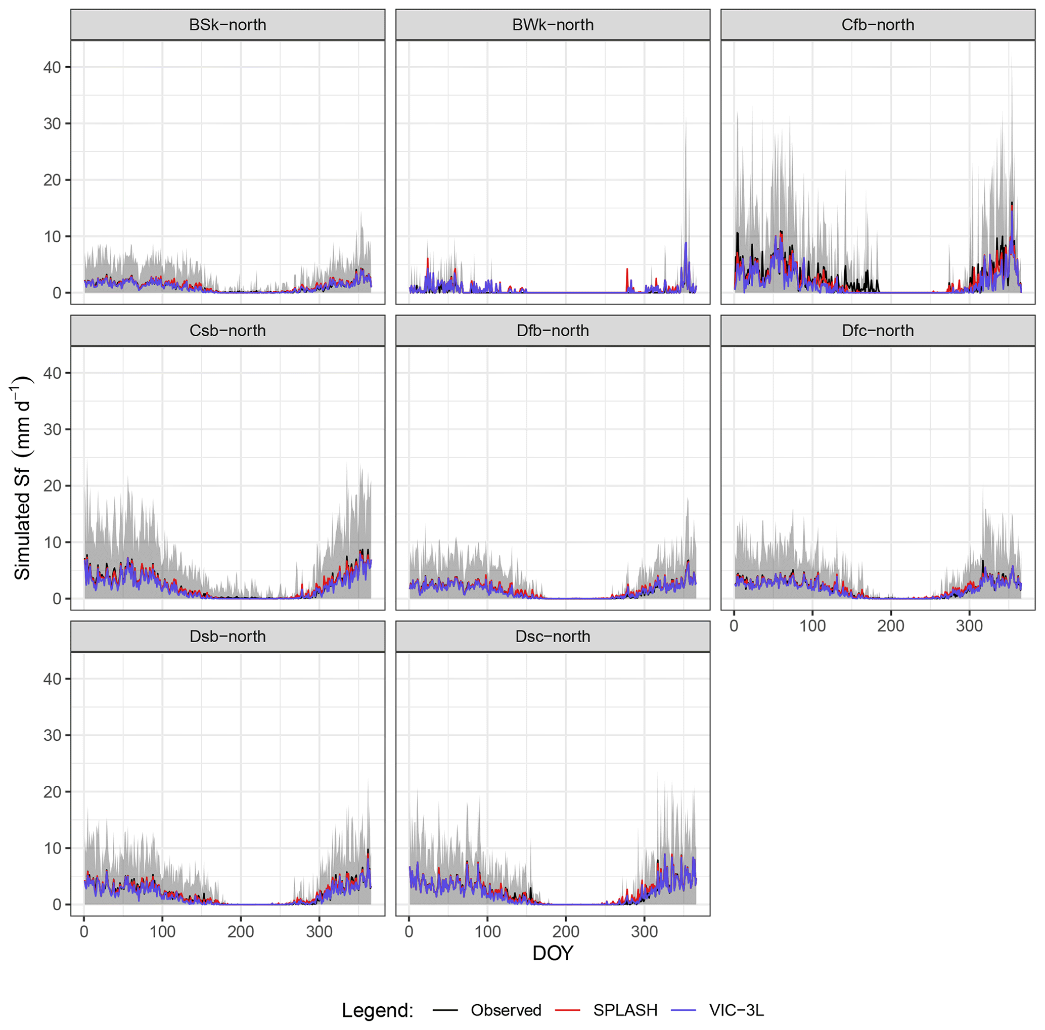
The seasonal patterns of Sf show differences in the magnitudes between climate zones with and without a dry season only in temperate types (Cfb, Csb), while wet continental (Df*) types did not show noticeable differences with their dry counterparts (Ds*). Arid climates (B*), on the other hand, showed the lowest magnitudes. The patterns simulated by SPLASH match the observations for all the climate zones almost perfectly, in agreement with the VIC simulations as well. Some underestimation is noticeable at the end of the winter in the wet temperate zone (Cfb) (Fig. 30).
6.2.6 Snowmelt
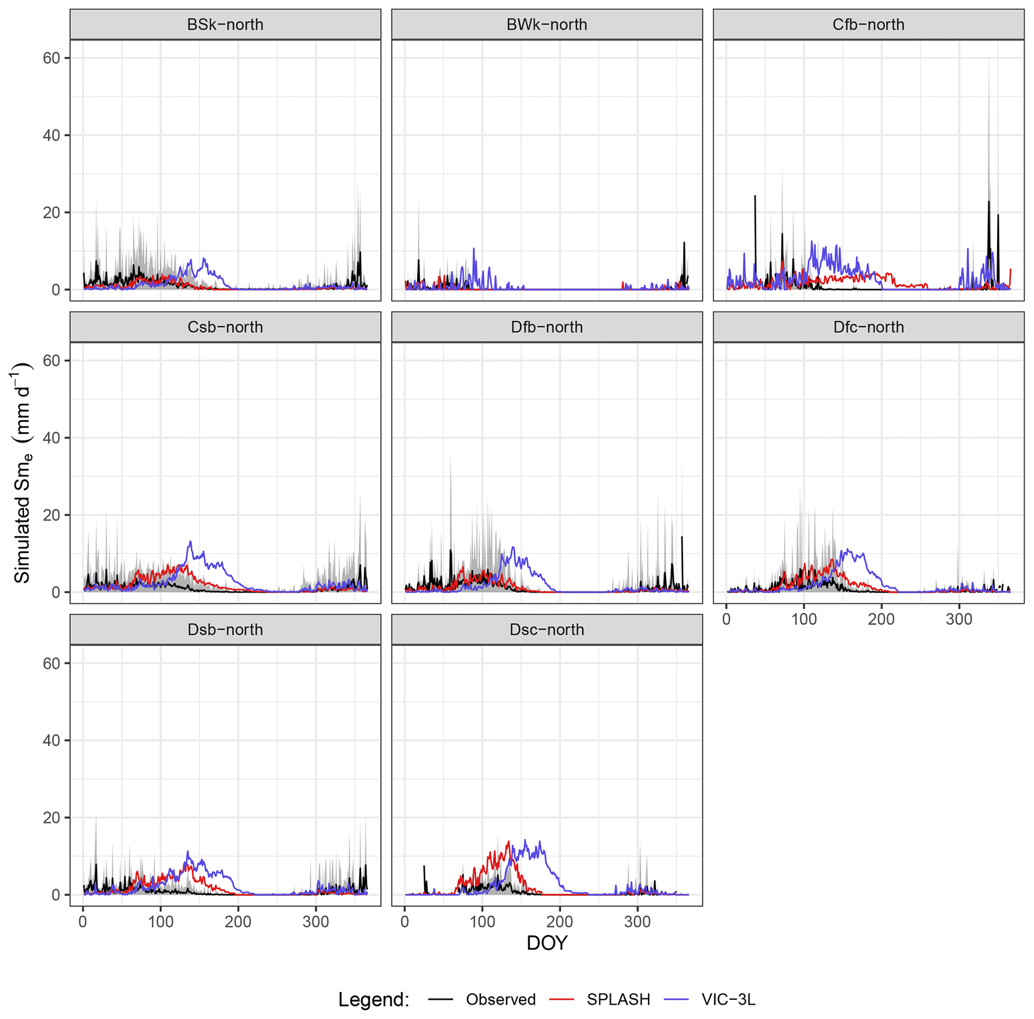
Seasonal patterns of Sm appear more clearly in the continental climate zones (D* types) with an expected peak at the beginning of spring; the other climate zones apparently do not show a general pattern. The SPLASH model was able to simulate the start of the melting process in all the climate zones; however, it captures the seasonal pattern only in wet continental climates (Df*), while overestimating Sm in their dry counterparts (Ds*). Overall the seasonal patterns from SPLASH seem to agree with the simulations better than the results of the VIC model, which shows a temporal lag at the start and peak of the melting period (Fig. 31).
6.2.7 Surface runoff and lateral flow
The SPLASH simulations of total streamflow (TSF) (RO+qout) in the watersheds were able to explain 71 % of the variation, while the estimations of surface runoff accounted for 69 % of the variation. The bias in both analyses shows a systematic underestimation of this flux, especially at the lower end (Fig. 32).
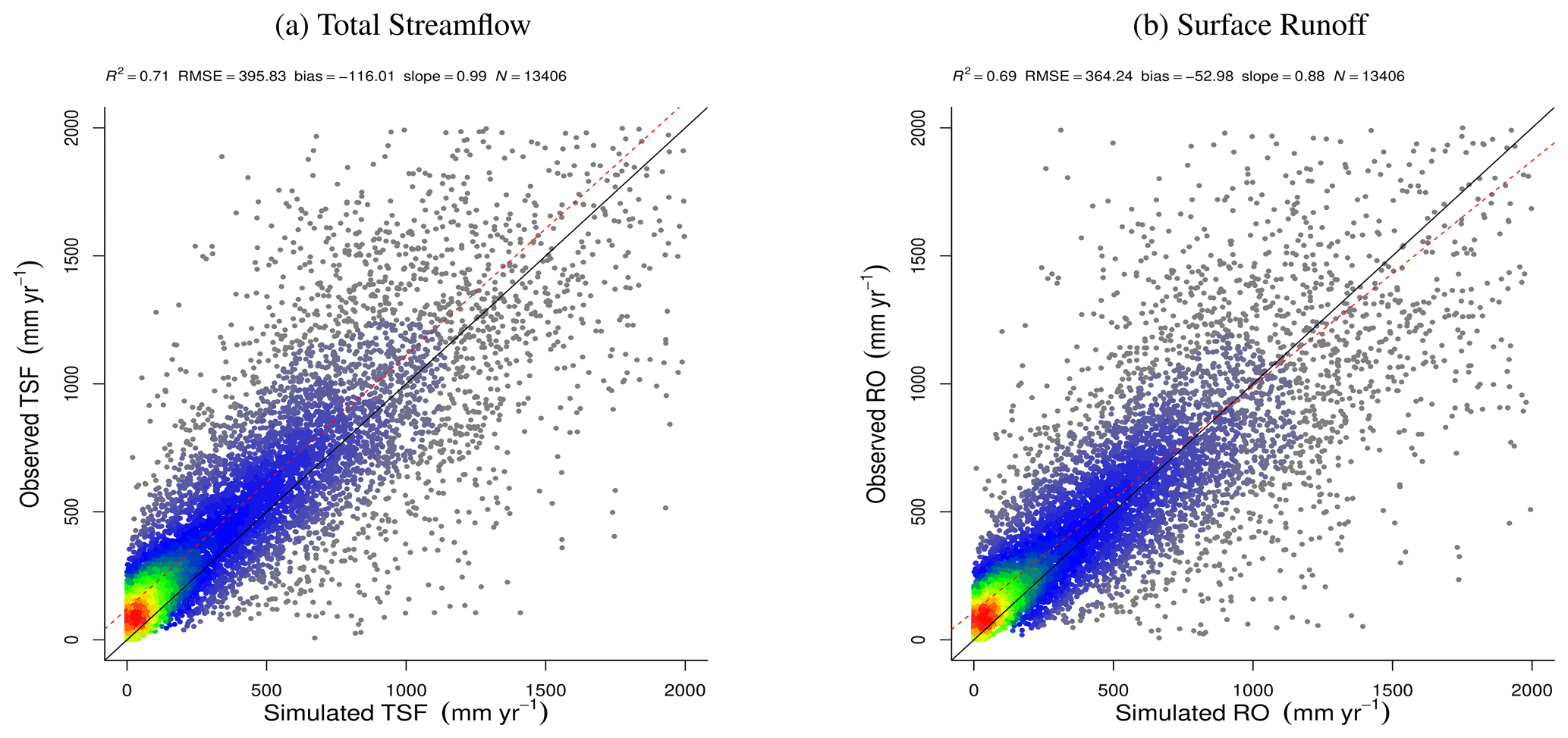
Figure 32Correlation of observed and simulated values of discharge with data from all the watersheds pooled. The color scale represents the plotted point density, where blue indicates lower densities and red indicates higher densities. (a) Total streamflow. (b) Surface runoff.
SPLASH simulations of TSF and RO in the same watersheds as VIC showed that although VIC achieved slightly better performance, SPLASH can achieve very similar R2 values. The slope of simulated vs. observed data suggests that SPLASH, without any local calibration, can reach 80 % of the accuracy of VIC calibrated with historical data (Fig. 33).
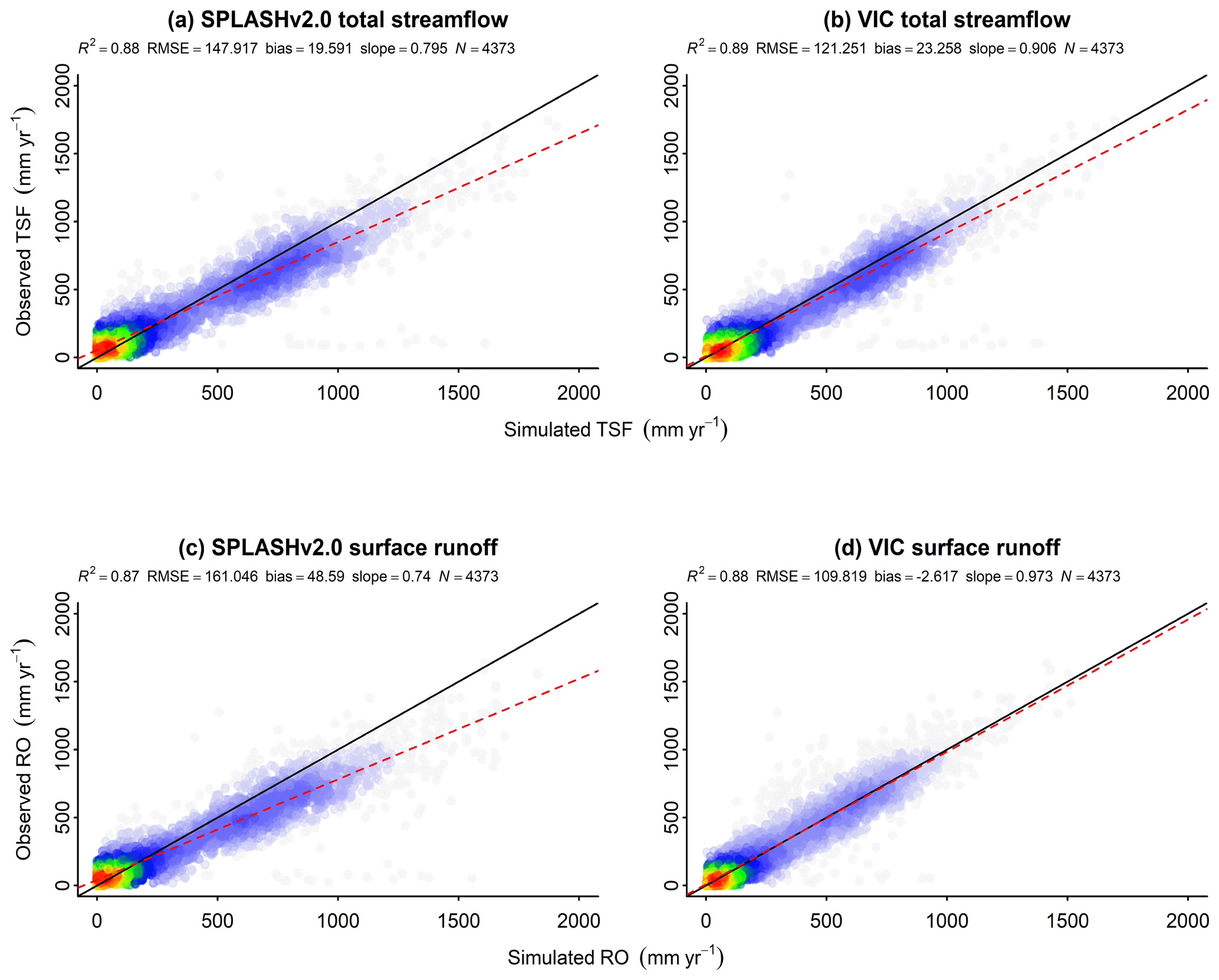
Figure 33Correlation of observed and simulated values of discharge with data from all the watersheds pooled. The color scale represents the plotted point density, where blue indicates lower densities and red indicates higher densities. (a) Total streamflow. (b) Surface runoff.
Tracking down the source of the systematic underestimation by analyzing the time series of observed and simulated TSF from Rietholzbach in detail, the underestimation appeared greater during winter months when the precipitation is below the average. On the other hand, when the precipitation is peaking, overestimation occurs in some years, seemingly without showing any systematic pattern (Fig. 34f).
The simulated time series of baseflow index BFI roughly follows the temporal dynamics of the observations. Overestimations appear in the winter months due to the underestimations of surface RO during these months (Fig. 34e). Furthermore, the spatial patterns resulting from the simulation show that the runoff is higher in areas surrounding the stream, which emerges from the flux accumulation at the valley bottom (Fig. 34b).
Moreover, the lateral flow is mostly produced in the north-facing slopes and in some areas next to the main stream, upslope from the main outlet. The BFI is close to 1 in most of the watershed, except in areas close to the stream, suggesting that most of the simulated hydrological response is subsurface flow (Fig. 34a).
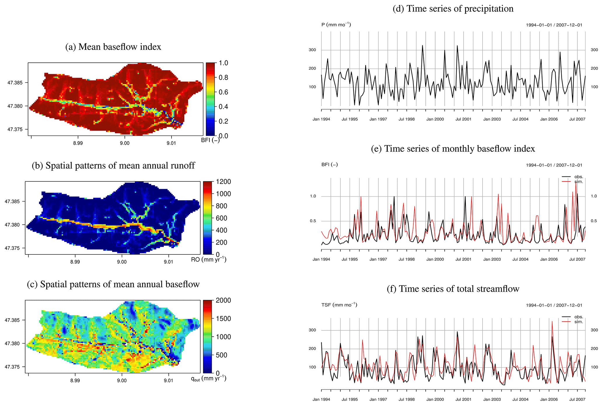
Figure 34Spatial and temporal patterns of runoff in a small wet temperate watershed in Rietholzbach, Switzerland. (a) Spatial patterns of mean soil water content in the first 2 m during 1994–2007. (b) Spatial patterns of mean annual runoff during 1994–2007. (c) Spatial patterns of mean annual baseflow during 1994–2007. (d) Time series of precipitation 1994–2007. (e) Time series of SWC in the first 1 m of depth during 1994–2007. (f) Time series of total streamflow during 1994–2007.
The monthly means of BFI from the long-term data from Rietholzbach suggest that the underestimation of surface RO is indeed systematic and the major discrepancies appear in November and December (Fig. 35).
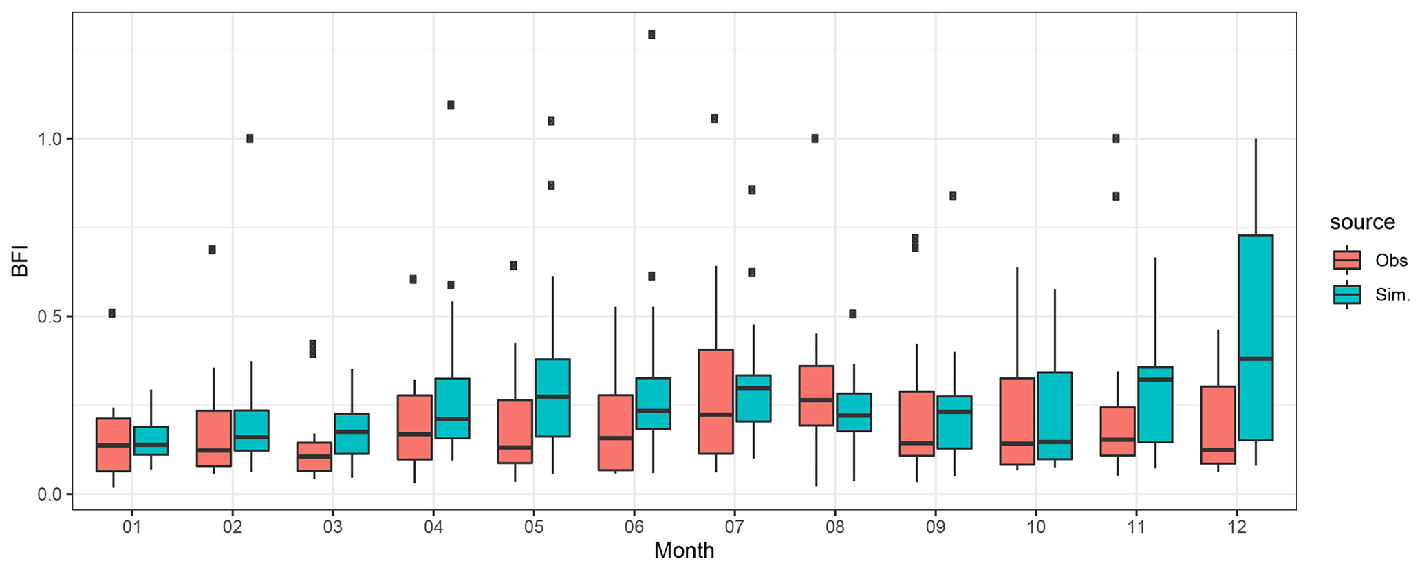
Figure 35Mean monthly BFI for 1994–2007 in a small wet temperate watershed in Rietholzbach, Switzerland, for the period 1994–2007.
At a daily time step, the results of the simulation in the tropical watershed show that the performance of SPLASH simulating fast storm response is poor, and the model fails in capturing the expected runoff peaks during relatively big storms at a daily timescale (Fig. 36e). Nonetheless, the spatial patterns generated by SPLASH in this small watershed reproduce mostly saturation excess runoff in areas close to the streams (Fig. 36a), while the simulated lateral flow appears stable spatially and over time (Fig. 36c and d).
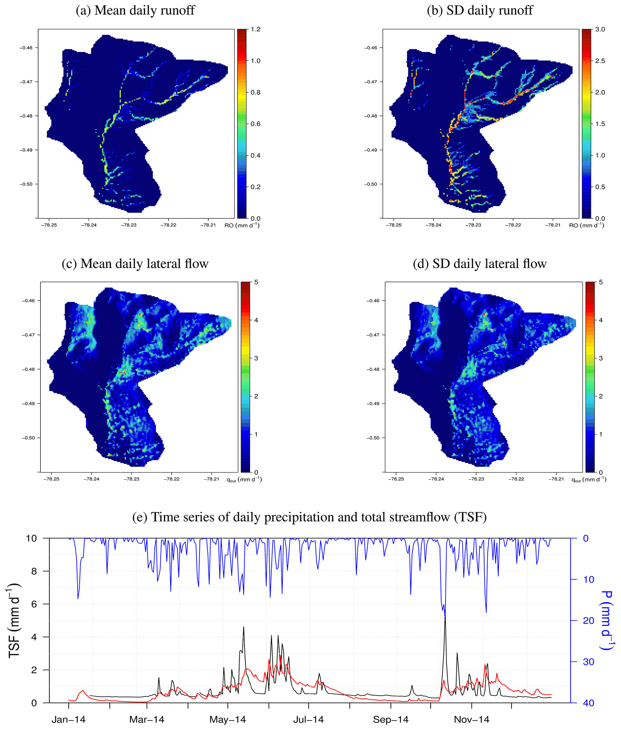
Figure 36Spatial and temporal patterns of daily fluxes in a tropical small watershed in Jatunhuayco, Ecuador. (a) Mean daily runoff during 2014. (b) Standard deviation of the daily runoff in 2014. (c) Mean daily lateral flow during 2014. (d) Standard deviation of the daily lateral flow during 2014. (e) Time series of daily precipitation and total streamflow during 2014.
6.3 Storages
6.3.1 Snow-water equivalent
The simple formulations proposed to simulate SWE were able to explain 88 % of the observed variation across 127 SNOTEL sites located in mountain regions. The mean value of the observations aggregated by biome shows that SWE in evergreen needleleaf forest (ENF) is the largest among the biomes, while the lowest value was from open–deciduous canopies (OSH, DBF). The bias suggests that SPLASH is underestimating SWE at low values; however, the huge variation of the observations in all biomes suggests that the differences are not significant (Fig. 37).
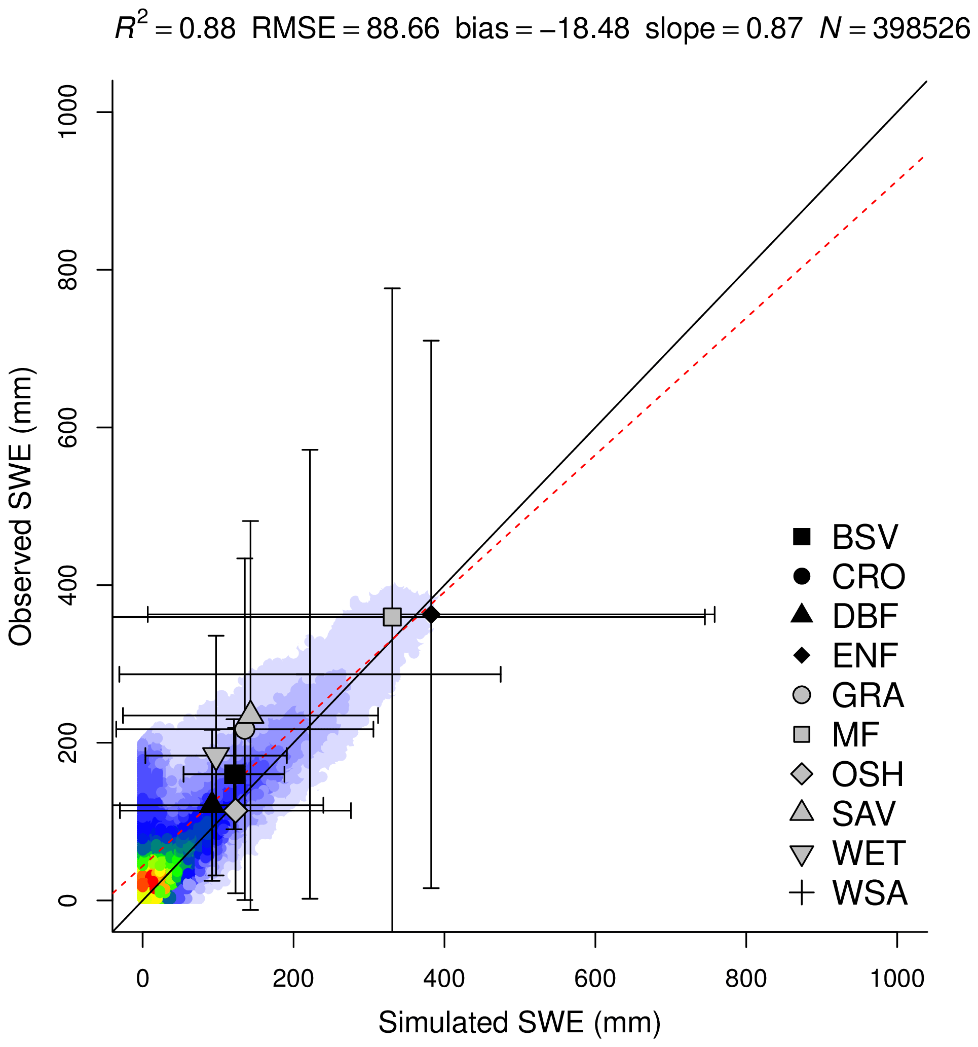
Figure 37Correlation of observed and simulated values of daily SWE, with values of all sites pooled. The color scale represents the plotted point density, where blue indicates lower densities and red indicates higher densities.
The seasonal patterns of SWE depict the well-known bell-shaped curve during winter with great deviations from the seasonal mean. Here, the sites in the temperate climate zones without a dry season showed the greatest deviation (Cfb). The SPLASH model was able to reproduce the seasonal patterns in all the climate zones. It underestimates, to different degrees, the averages within the range of the observations, which contrasts with the overestimation of the VIC simulations. Nonetheless, SPLASH captures the length of the snow-covered period almost perfectly, failing only in the Cfb zone, where it overestimates SWE during the melting period; here VIC outperforms SPLASH (Fig. 38).
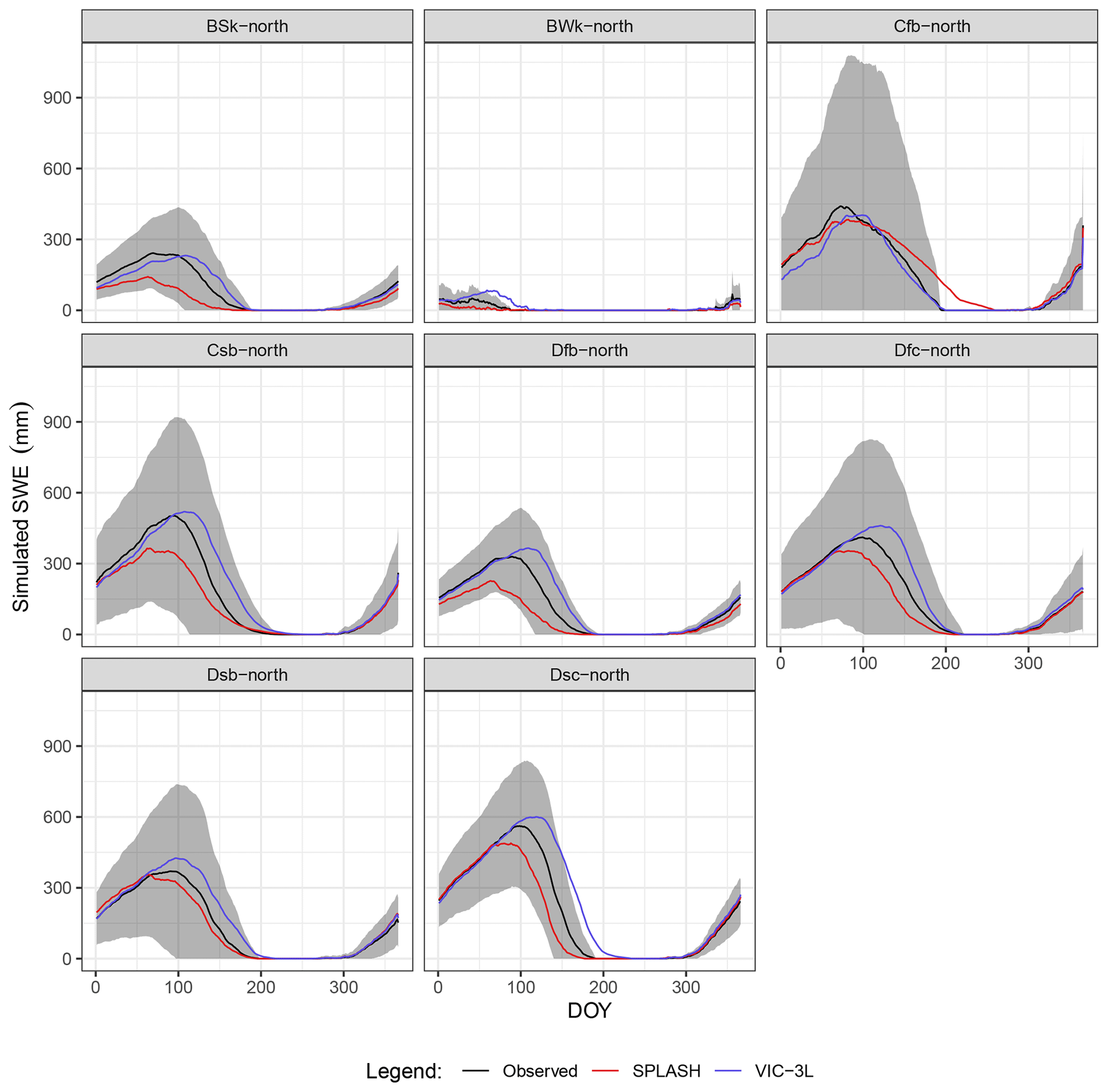
Figure 38Mean seasonal cycle of SWE per climate zone. The gray areas show 1 SD from the observed mean. Climate zones are described in Table A3.
The spatially distributed high-resolution simulation over North America showed strong patterns defined by the topography, with higher SWE over the mountain regions and variations according to the slope exposure. A well-defined lower boundary for the snow-covered area emerged in the eastern US around 40° of latitude, coinciding with the transition from climates Cfa to Dfa, while on mountain summits the simulated SWE fades at around 35° (Fig. 39).
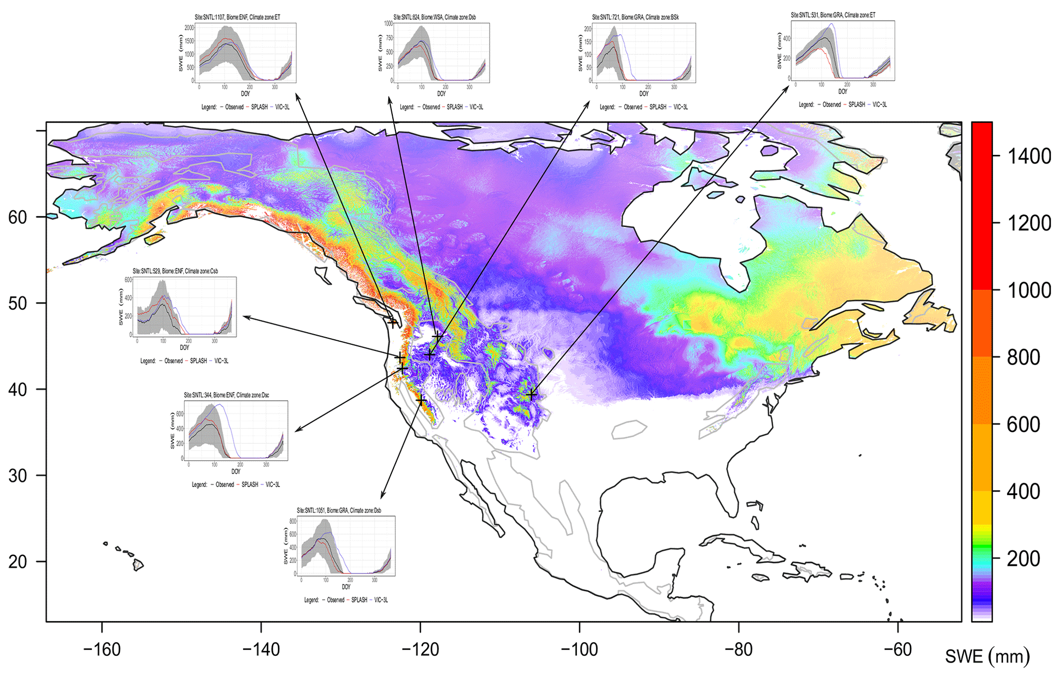
Figure 39Spatial patterns of mean monthly maximum SWE for the period 2010–2016 over North America at 1 km resolution, along with site simulation examples from the mountains. The gray areas show 1 SD from the observed mean.
6.3.2 Soil water content
The performance evaluation of daily SWC was done with data from stations measuring soil moisture deeper than 30 cm located in the mountain regions, resulting in 16 EC (Fig. 40a) and 127 SNOTEL (Fig. 40b) stations. Comparison among biomes was not possible due to the different depths of measurement at each station. This shows, for example, because of mostly superficial measurements, wetlands at the lower end of the observation axis (Fig. 40b). Nevertheless, the SPLASH model was able to explain 86 % of the variation in the EC dataset, which is around 7 times smaller than the SNOTEL dataset where SPLASH explained 54 % of the variation. The evaluation also shows that SWC was overestimated by the SPLASH model in grassland ecosystems (GRA) and in open shrublands (OSH) (Fig. 40).
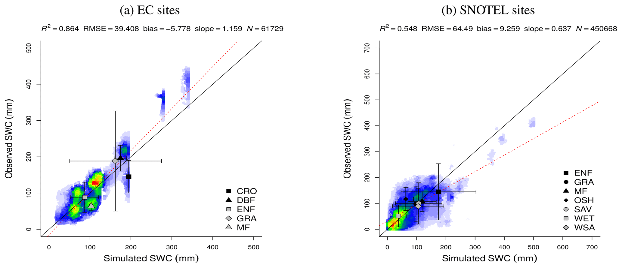
Figure 40Correlation of observed and simulated values of daily SWC, with values of all sites pooled. The color scale represents the plotted point density, where blue indicates lower densities and red indicates higher densities.
The seasonal patterns of Θ, extracted from the data and simulations at SNOTEL sites, show a sinusoidal shape in all the climate zones. The highest point appears during the first half of the spring and the lowest point by the end of the summer. Most of the climate zones show huge deviations from the mean, especially the zones without a dry season (e.g., Cfb, Dfc), except for the cold desert (BWk) where this variation is smaller.
The SPLASH model shows reasonable agreement of the seasonal pattern for climate zones with warm and dry summers (i.e., Csb, Dsb) and for the cold steppe (BSk). In these climate zones, SPLASH reproduces the seasonality in a better way than VIC.
In some continental climates (Dfb, Dfc, Dsc), SPLASH produces a similar pattern to the observed mean but downshifted inside the expected deviation. In these climate zones, the VIC model approaches the observed mean only during spring–summer months. In the warm-summer temperate climate with no dry season (Cfb), SPLASH is not able to reproduce the seasonal pattern, and the amplitude of the sinusoidal shape is too small to match the observations. Here, VIC agrees with the observations briefly during winter. In the cold desert (BWk) SPLASH does not produce a seasonal pattern, and the average through the year remains close to the minimum. Here VIC overestimates Θ during spring and produces negative values during the spring and summer months (Fig. 41).
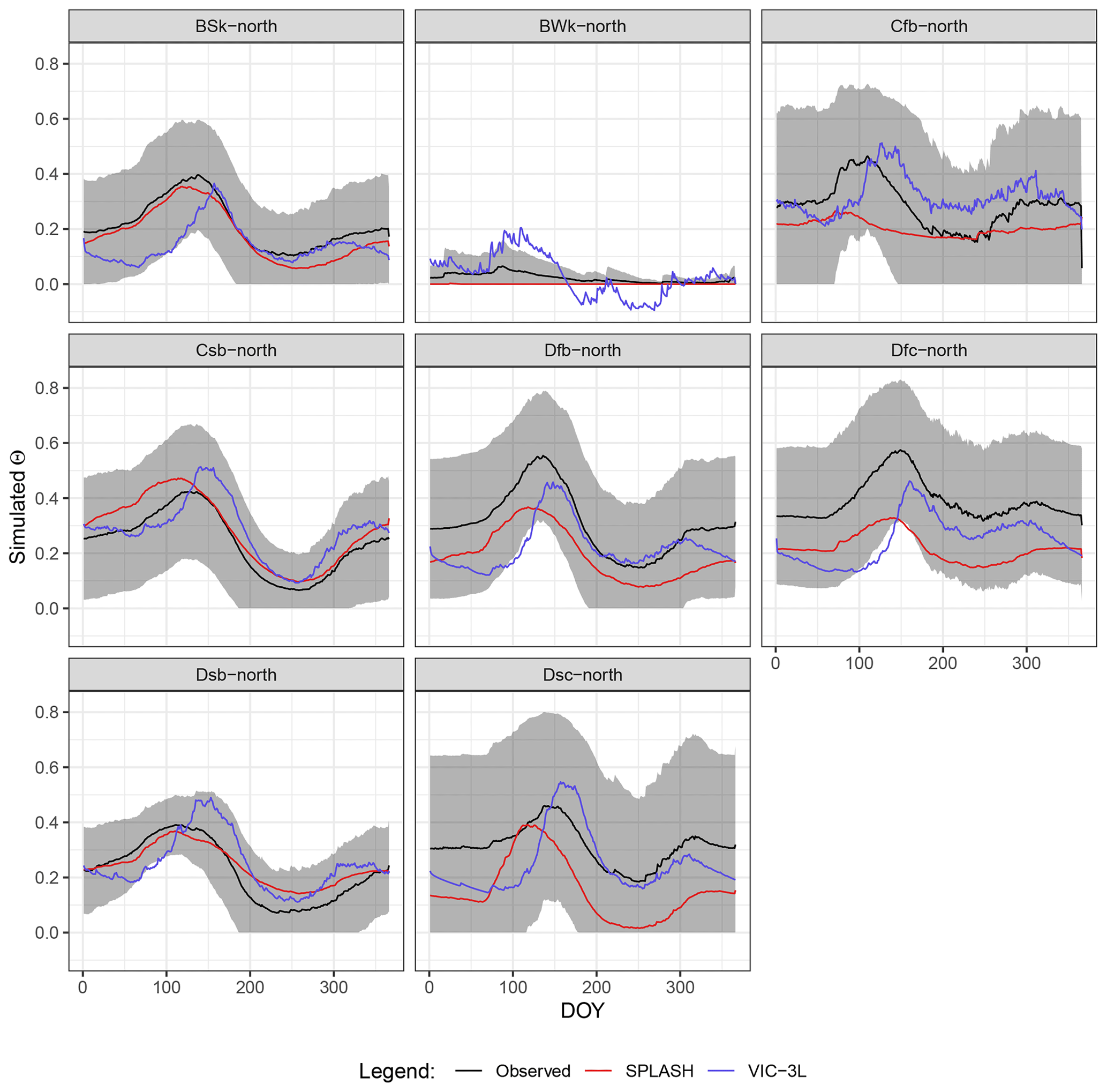
Figure 41Mean seasonal cycle of Θ per climate zone. The gray areas show 1 SD from the observed mean. Climate zones are described in Table A3.
The spatially distributed simulation of relative soil moisture saturation shows that the patterns of the annual average roughly follow the global climate zone distribution. At this resolution, the model was incapable of reproducing the streams and most of the mountain regions emerged as areas half- to low-saturated (Fig. 42).
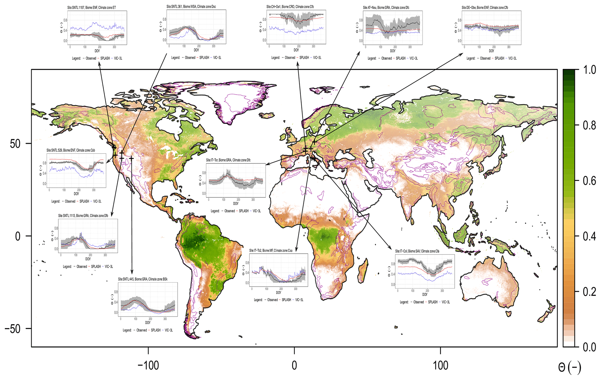
Figure 42Spatial patterns of mean annual Θ for the period 2010–2016 at 5 km resolution along with site simulation examples from the mountains. The gray areas show 1 SD from the observed mean.
The spatial patterns of the total soil water content in the temperate watershed show an emergent accumulation at the valley bottom, shaping the stream. Here, the SD is very small, suggesting that the valley bottom remains wet most of the year (Fig. 43d).
The different patterns over north- and south-facing slopes show the former with more water content over the latter but more variations over time. The emergent variations in the north-facing slope are shaped by the inclination of the slope, while on the south-facing slope, this pattern seems to follow the aspect (Fig. 43c).
The time series of soil water content over the first meter of depth was poorly reproduced by SPLASH, and in some years the simulation matches the observations (e.g., 2006); however, in most of the years the droughts are underestimated and the peaks are overestimated (Fig. 43e).
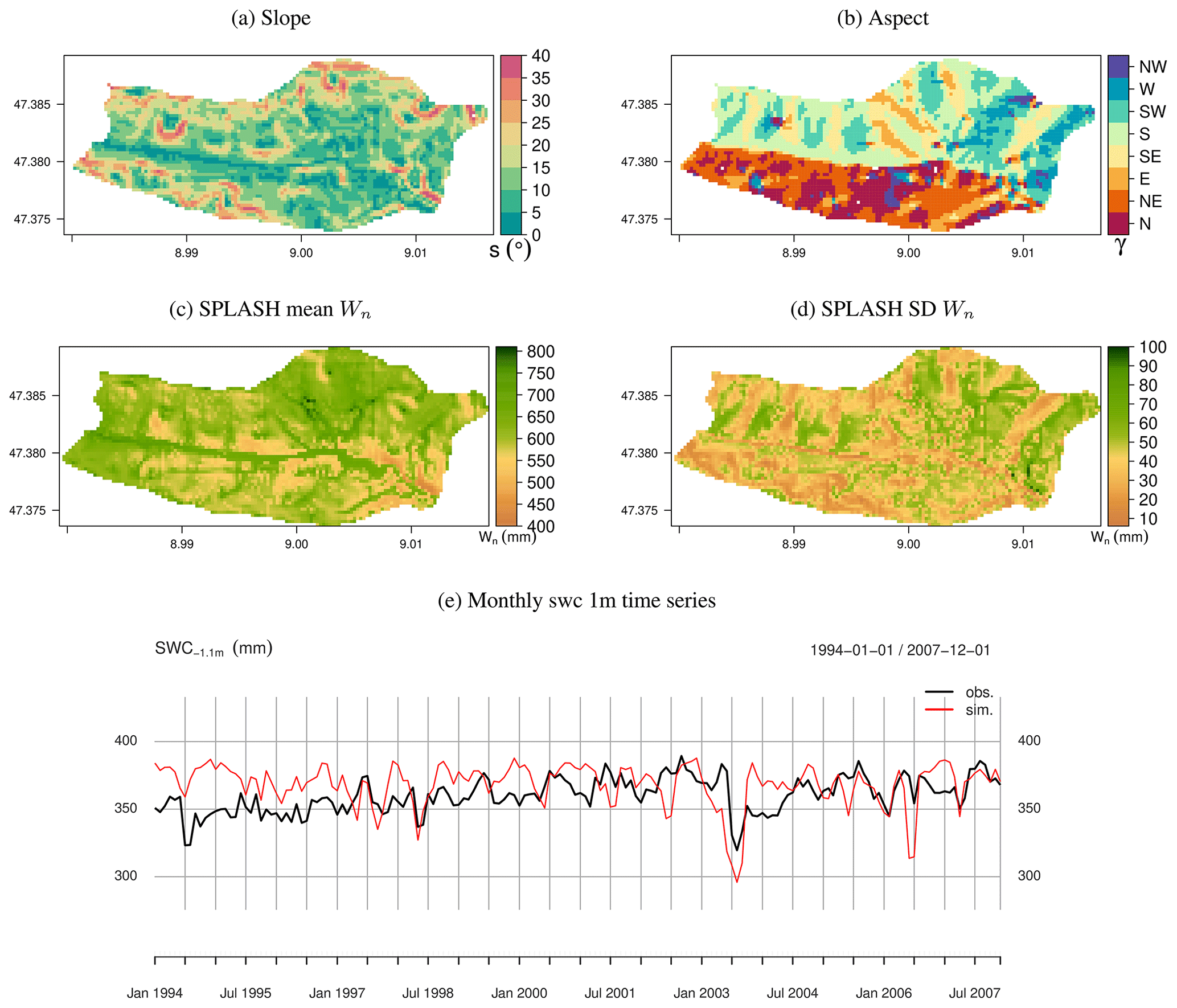
Figure 43Spatial and temporal patterns of soil water content in a small wet temperate watershed in Rietholzbach, Switzerland. (a) Slope in degrees. (b) Slope orientation; N stands for north, S for south, and so on. (c) Mean annual simulated soil water content in the whole column during 1994–2007. (d) The standard deviation of the daily soil water content in the whole column during 1994–2007. (e) Time series of monthly soil water content, simulated and observed over the first 1 m of depth.
In the tropical watershed, the spatial patterns of the daily average Wn show the emergent stream at the valley bottom; according to the simulations the daily water content here is more variable than in the rest of the watershed (Fig. 44d), contrary to the temperate watershed where this pattern was opposite. Here the east–west aspects define the spatial patterns, and the eastern flanks show less water content than their western counterparts (Fig. 44c).
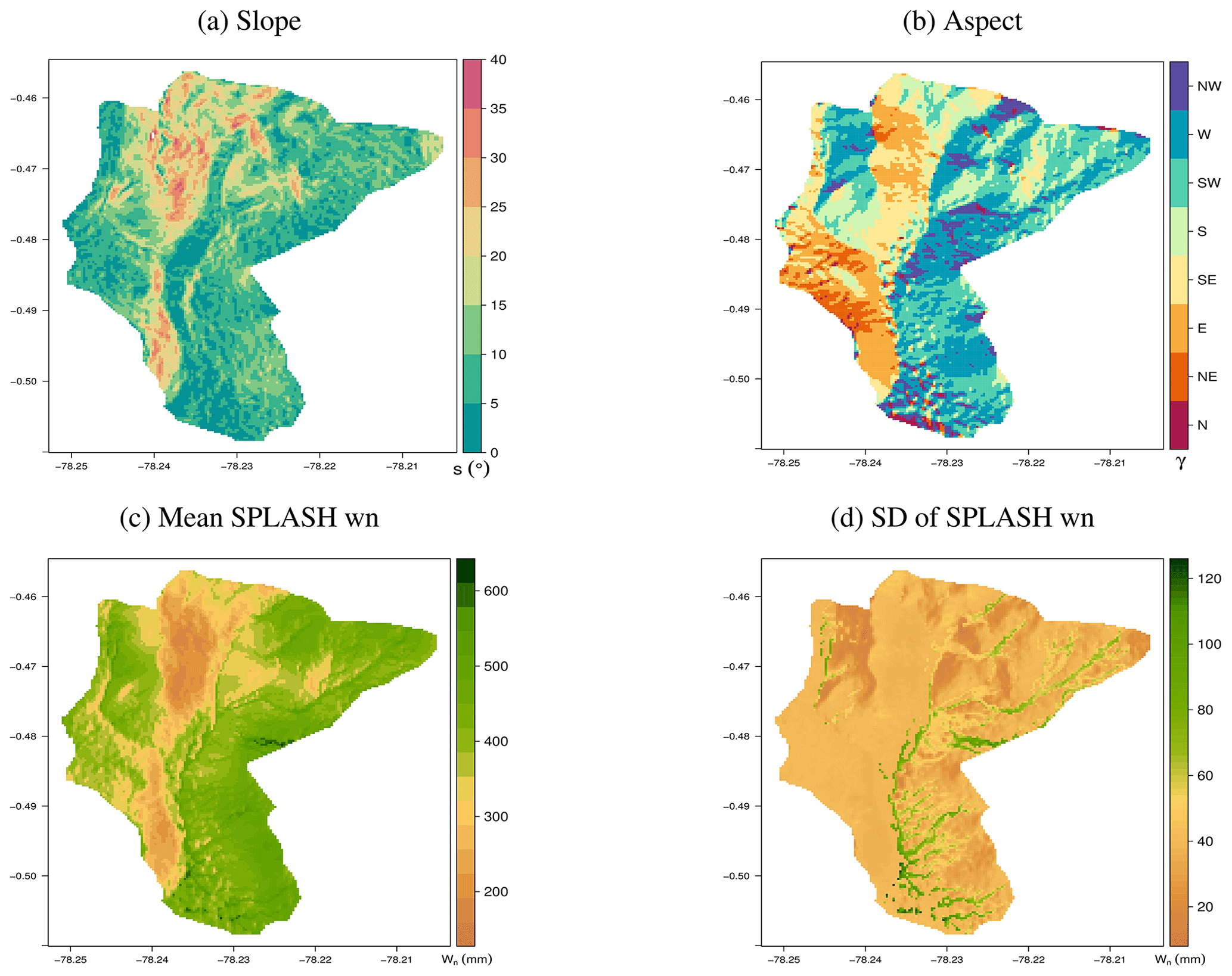
Figure 44Spatial patterns of daily soil water content in a wet tropical watershed in Jatunhuayco, Ecuador. (a) Slope in degrees. (b) Slope orientation; N stands for north, S for south, and so on. (c) Mean daily soil water content during 2014. (d) Standard deviation of the daily soil water content during 2014.
The updated SPLASH model showed reasonable agreement with the observations in all the fluxes analyzed here without any local calibration or prescribed land cover information. The data requirements to run the model (precipitation, solar radiation, air temperature, elevation, and soil texture) are modest; the open-source code, compiled in a ready-to-use package, facilitates replication.
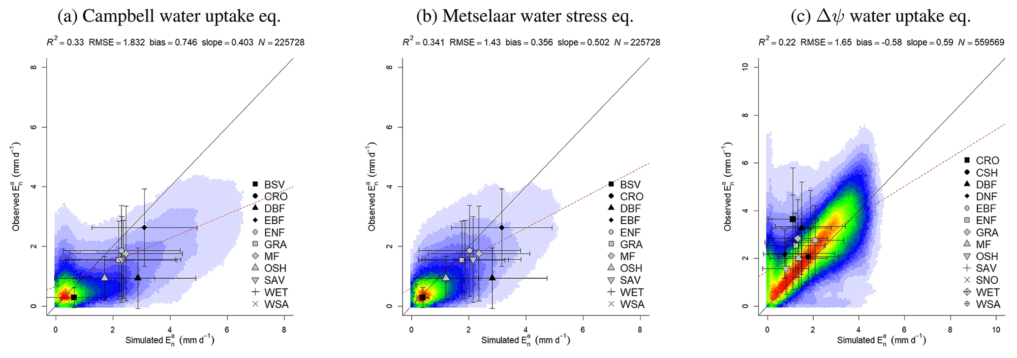
Figure 45Simulation experiments against EC observations using different soil water stress and water uptake functions. The color scale represents the plotted point density, where blue indicates lower densities and red indicates higher densities. (a) Using the Campbell and Norman (1998) water uptake function at mountain sites. (b) Using the Metselaar and de Jong van Lier (2007) water stress function and a constant Sc=1.05 (mm h−1) (Federer, 1982) at mountain sites. (c) Using the gradient of water potential soil-leaf Δψ to drive the water uptake in the entire FLUXNET database.
The analytical approach used to solve the energy and water fluxes allowed the model to run with high-resolution data on global scales without using statistical–dynamical flux parameterizations or hydrological unit responses. Emergent patterns produced by the model follow the natural accumulation of soil moisture downslope. Most of the fluxes and storages analyzed here agree with – and sometimes outperform – the more complex VIC-3L model, which was chosen for comparison due to its wide use in ecohydrological applications and its well-known good performance.
SPLASH assumes background albedo, a parameter particularly crucial due to its synergy with water fluxes, to be constant for all biomes. This contrasts with the VIC model, which uses monthly albedo per vegetation class (Gao et al., 2009). Nonetheless, SPLASH showed overall good agreement of with the observations, suggesting that the snow effect on the albedo is much stronger than the effects of the phenology in snow-covered regions (Xiao et al., 2017). This global albedo assumption, however, is more likely to be the cause of the discrepancy of in ecosystems with sparse vegetation cover (e.g., BSV and OSH), where the extent of exposed soil and its moisture status modify the albedo (Campbell and Norman, 1998; Barry, 2008).
Although the ground heat flux is ignored by the model, an improvement in the calculation of is noticed relative to the previous version (Davis et al., 2017), where the overestimation in the arid desert (BWh) is fixed with the new parameterization of the longwave radiation and the overestimation in the polar tundra (ET) is corrected by the new included feedback of snow albedo.
Simulated actual evapotranspiration () is underestimated to various degrees in all biomes. As model performance for is high, this suggests that the discrepancies are related to the empirical parameterization of the water supply and uptake (SW). Theoretically, this should be driven by the soil-to-leaf-water potential gradient (Δψ) (Prentice et al., 2014), thus reflecting different plant strategies to deal with drought. However, when this idea was tested during the development stage, the performance of the simulations decreased (Fig. 45c), probably due to the calculation method used for the leaf water potential and its assumptions (both taken from the literature): the canopy well coupled to the atmosphere at pre-dawn (thus Ts=Ta) and the relative water content of the leaf close to saturation (Appendix A4).
Although in this version of SPLASH, we propose a physically based calculation for the upper threshold of SW, its response to the water deficit is conceptualized as a linear function, which has been reported as the most simple and reasonable empirical description (e.g., Federer, 1982). Nonetheless, several authors report more complex formulations depicting convex (Campbell and Norman, 1998), concave (Metselaar and de Jong van Lier, 2007), or trapezoidal (Feddes and Raats, 2004) shapes. Some of these formulations were tested during the development stage of the model, with no significant improvement over the simple linear formulation (Fig. 45).
From this experimentation, the assumption made on the maximum supply rate Sc as the maximum rate of evaporation yielded the best approximations. This assumption makes more sense in bare-ground areas; however, in vegetated areas, this value should reflect the plant controls on transpiration, which ideally needs to be addressed with ideas based on eco-evolutionary optimality theory (Harrison et al., 2021).
Since SPLASH seems to reproduce the evapotranspiration better over non-water-limited areas, in such areas, slopes facing the Equator (south-facing slopes in the Northern Hemisphere) should, in theory, show higher values than their opposite-facing counterparts, which receive less radiation (Körner, 2021; Chapin et al., 2011).
This spatial pattern is indeed produced by SPLASH in the Rietholzbach experimental catchment. However, here the latent heat calculated from the Landsat 5 retrievals does not show any strong differences between north- and south-facing slopes. It is still unclear if the spatial patterns from Landsat are correct; the SEBAL algorithm used the calculate LE is limited to clear-sky pixels only, and thus a large amount of data was excluded from the calculation. Furthermore, this algorithm computes an instantaneous (at the satellite overpass), and then it assumes this proportion is constant through the day, so the daily Ea can be calculated from the daily accumulated Rn measured on the ground (Bastiaanssen et al., 1998a). Therefore, a more accurate estimation from SEBAL would involve terrain-corrected independent calculations of Rn at Landsat spatial resolution, which were unavailable at the time of this comparison. Land use in Rietholzbach also plays a key role in shaping the spatial patterns of LE.
SPLASH in theory reflects the environment the plants experience. The spin-up routine produces an initial state of equilibrium, and thus in areas with natural vegetation the spatial patterns produced by SPLASH should reflect this vegetation cover to some degree. This is shown in the agreement (to some extent) of the spatial patterns of produced by SPLASH compared with the Landsat 8 LE in the tropical watershed, which always had natural vegetation. This microclimatic gradient created by the slope and aspect is particularly important to explain outlier populations existing beyond their major distribution zone, which can colonize their surroundings during rapid climatic changes (Chapin et al., 2011).
Although the results presented here are encouraging, more rigorous comparisons are needed to evaluate how well the fluxes produced by SPLASH reflect patterns of naturally occurring vegetation.
The less-than-optimal performance of SPLASH simulating condensation is mainly due to the lack of other environmental variables needed to calculate the dew point and surface temperature, such as air humidity, wind speed, and aerodynamic resistance. Nonetheless, the simple assumption made to estimate this flux (10 % of ) reproduces the seasonal Cn better than VIC. The major discrepancies of VIC's Cn happen during the spring–summer months, suggesting that some of the heat lost as Cn (latent) is actually lost from the surface by convection, cooling the leaves. The yearly magnitudes of dew formed by Cn suggest that its impact on the water balance is minimal in most climate zones, except for hot arid climate zones (BSh), where Cn has ecological importance, in agreement with the observations reported by Guo et al. (2016) and Yu et al. (2020).
The size of the snowpack (SWE) simulated by SPLASH agrees more than 80 % with the observations; however, its seasonal patterns show a systematic underestimation in most of the climate zones. Since the seasonal patterns of the snowfall (Sf) produced by SPLASH match the observations in all the climate zones, the snowmelt (Sm) is reasonably well predicted in the steppe (BSk) and the wet continental climates (Df*). In these climate zones, the discrepancies seem to be due to the redistribution of snow by the wind, which is greatly dependent on the structure of the vegetation (Barry, 2008; Pomeroy and Brun, 2001) and is not considered by the model. In dry continental and temperate climates (Ds*, Csb), on the other hand, SPLASH systematically underestimates SWE. Here the cause is more likely to be neglecting the “cold content” of the snow, which in turn causes an overestimation of Sm. This effect is stronger at high elevations where the temperature is lower; here VIC delivers better estimations than SPLASH (Fig. 45). Moreover, despite the discrepancies in the simulated magnitudes at these sites, the duration of the snow-covered period is reasonably predicted, considering that the multi-annual variation can be up to 1 month (Körner, 2021).
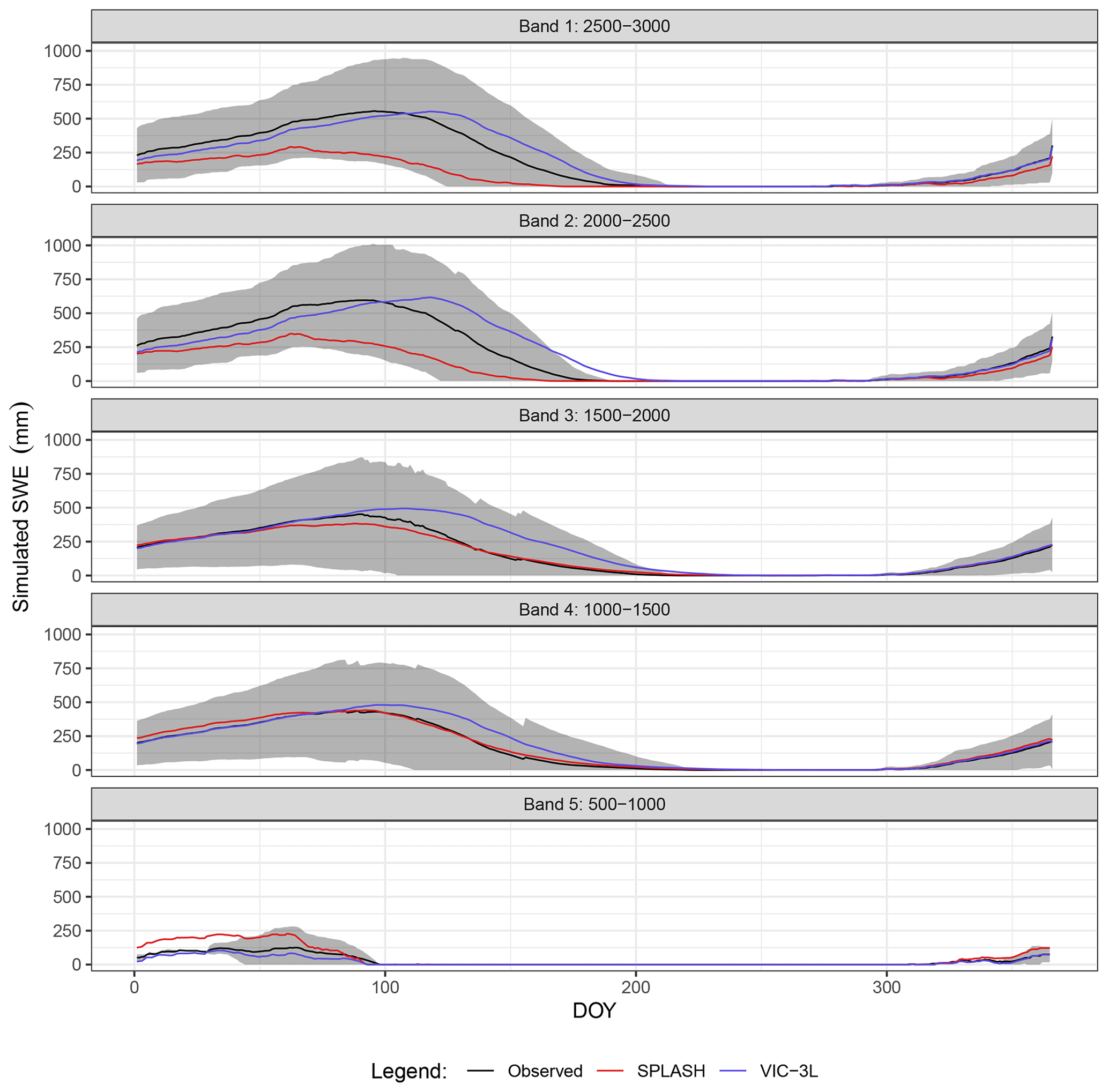
Figure 46Mean seasonal cycle of SWE over dry temperate climates (Csb) per elevation band. Results aggregated every 500 m a.s.l. The lines show the means, while the gray shaded area shows the SD.
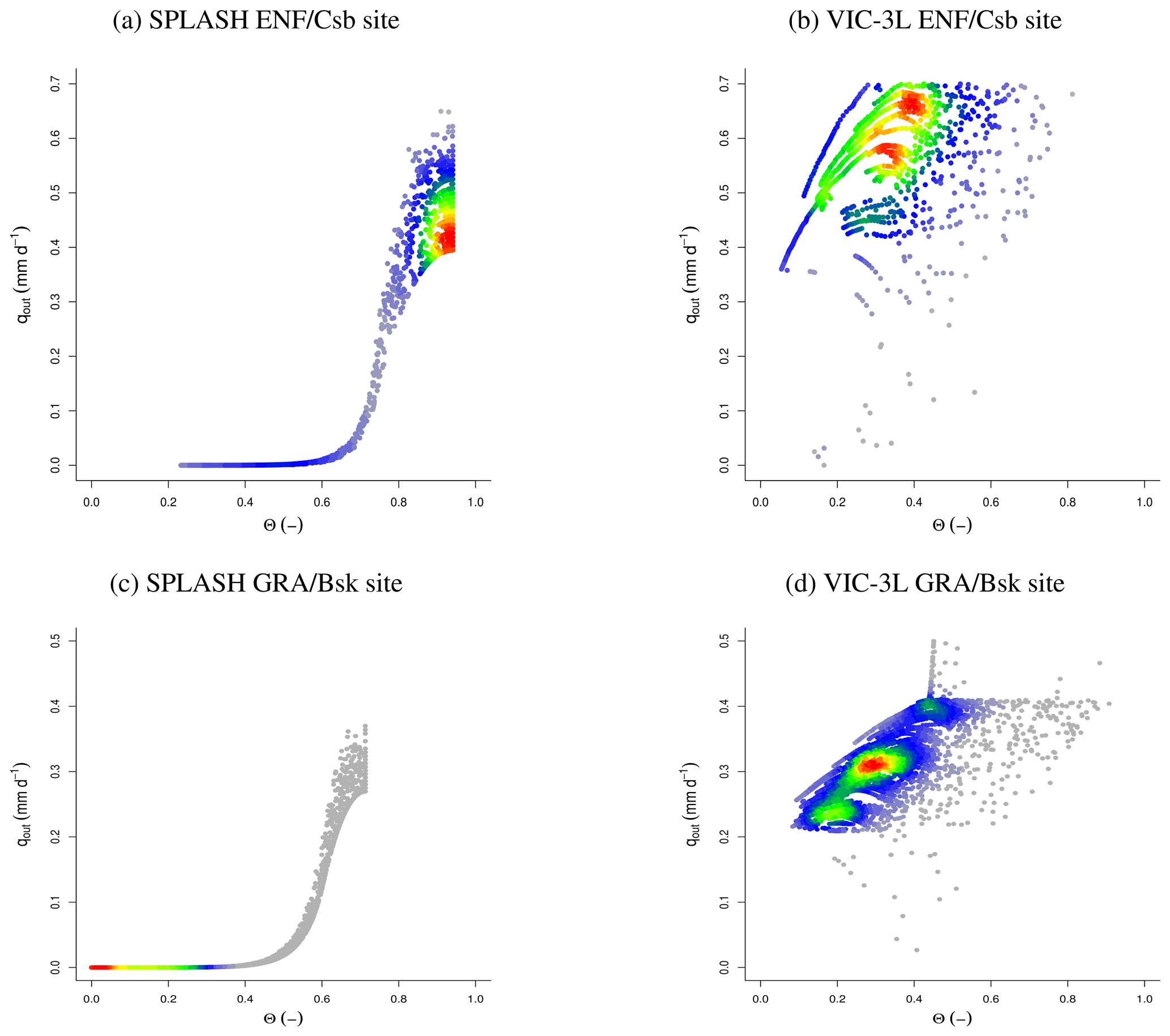
Figure 47Emergent response of the lateral flow to soil moisture from an ENF in a temperate climate, with a dry and warm summer (Csb) (site SNTL:529), simulated from (a) SPLASH and (b) VIC-3L. The same relationship from a GRA in an arid cold steppe (Bsk) (site SNTL:871), simulated from (c) SPLASH and (d) VIC-3L.
Although in theory, different sets of parameters in the snow albedo functions, depending on the complexity of the canopy, should yield more accurate predictions (e.g., Romanov, 2003), the performance of SPLASH simulating SWE shows that one set of parameters is able to deliver reasonable approximations for all types of biomes. Such an approximation was possible using roughly 106 of RS and ground data points spawned over 15 years at 315 stations during the optimization process. The use of one set of parameters is nothing new and has been done for a long time; however, in previous studies, the number of observations and available tools limited the spatial representativity of these calibrations (Clark et al., 2017). Nonetheless, the parameters found in SPLASH for the snow albedo decay function are consistent with the values proposed in the Noah model by Livneh et al. (2010), although in SPLASH there are no different sets of parameters for accumulation and melt seasons.
The spatial patterns of the surface runoff generated by SPLASH in the small watersheds show that most of this flux is generated in the saturated zone in the valley bottom, in agreement with what is expected in montane regions (Grayson and Blöschl, 2000; Weizu and Freer, 1995).
Moreover, the spatial patterns of BFI produced by SPLASH in Rietholzbach agree with previous studies which show that most of the streamflow is produced by subsurface flow, especially interflow (Von Freyberg et al., 2014; Gurtz et al., 2003). However, the poor performance of SPLASH simulating the daily surface runoff in the Andean catchment suggests that the assumption made for the event duration does not hold for this area, or the saturated zone close to the stream, which controls this flux in Andean catchments (Correa et al., 2020), is underestimated.
Although the simulations of soil moisture are overall reasonable and the results mostly matched the temporal dynamics of the observations, two recurrent errors were observed among the simulations (or a combination of these errors): the resultant soil moisture appears up- or downshifted randomly (first error), or the amplitude of the variations is different from what is observed (second error).
The first type of error seems to be related to the estimation of the bucket size, which in turn is defined by the pedotransfer functions and soil data. Although the pedotransfer functions were optimized with a global dataset, which covers a wide spectrum of textural classes with a wide range of SOM combinations, the empirical nature of these equations is a well-documented source of error (Pachepsky et al., 2015; Van Looy et al., 2017; Paschalis et al., 2022). This error might explain why the evapotranspiration and total streamflow agree with the observations in Rietholzbach, but the performance of the soil moisture simulation was very poor.
The second type of error was less recurrent with the SNOTEL dataset, which includes actual measurements of soil properties, suggesting that the data obtained from SoilGrids for the EC sites might be a source of this error. The coarser volumetric fraction (stoniness) in particular can reduce the size of the bucket dramatically here. However, a rigorous evaluation and sensitivity analysis are needed to define this source of error in a broader modeling context.
The spatial patterns of soil moisture at a global scale show how the assumption of the model of a maximum depth breaks the hydrological connectivity in large watersheds. Here, the model forces the water to flow down instead of laterally if the bedrock is not in the first 2 m of depth. On the other hand, in small watersheds, the hydrological connectivity emerges from the conceptualization of the model accumulating the moisture at the valley bottom and shaping the streams.
Furthermore, the lateral flow simulated by SPLASH is strongly related to the soil water content, consistent with what has been reported in Rietholzbach (Teuling et al., 2010) and in Andean watersheds (Crespo et al., 2011).
The exponential decay of the saturated conductivity with depth, widely used in TOPMODEL-type models, was deliberately excluded from the model. The saturated hydraulic conductivity is highly dependent on the organic matter content and was calculated using a weighted average (by depth) of SOM as an input. Since SOM generally decreases exponentially with depth (Kramer and Gleixner, 2008; Hobley and Wilson, 2016; Bai et al., 2016) this estimated Ksat should be reproducing the decay to some degree. However, the available data used for the optimization of the pedotransfer functions calculating Ksat were biased towards sandy and loamy-sand soils, affecting the performance in the rest of the textural classes.
The lateral flow equation proposed here is based on the profile transmissivity, originally proposed by TOPMODEL and the assumption of steady-state flow. However, it has been reported that the steady-state flow assumption holds better in wet catchments with high hydraulic gradients. In dry catchments or during dry periods, areas of the catchment may lose their hydrological connectivity (Woods et al., 1997; Tague and Band, 2001).
Analyzing the response of the lateral flow to soil moisture generated by SPLASH, the minimum qout reflects stable gravity-driven drainage (which in shallow soils defines the baseflow), while the maximum qout appears as pulses resulting from individual precipitation events, mimicking the behavior of the interflow (Fig. 47a). This response is consistent in both wet and arid sites, albeit with varying magnitudes (Fig. 47c).
In VIC3-L, however, qout reaches values of the order of hundreds (truncated in the figure), while soil moisture is not even saturated (Fig. 47b). In the comparable region of the analysis, the upper envelope of the scattered points shows a linear threshold and a sharp transition to a plateau. The flux here seems to display relatively high values when the soil moisture is close to the wilting point, which is theoretically impossible.
Despite the limitations discussed, the updated SPLASH model provides fast and parsimonious means to generate robust estimates of water and energy budgets across regions, regardless of their topographic complexity and spatial scale. The calibration-free approach enhances the model’s portability and the ecological interpretability of the results. Moreover, since the structure of the model contains fewer moving parts than any other LSMs, it facilitates formulating ecologically driven working hypotheses on why results do not match the observations in the case of big discrepancies. With targeted refinements, SPLASH could become an even more robust tool for ecohydrological modeling and for exploring hydrological impacts of global change.
A1 Recession constant
Analyzing the flux from one cell, according to the linear reservoir model (Eq. 42) and the BC model (Eq. 39), the maximum (initial) lateral flux will happen when the soil is saturated. In the same way, it will be close to zero at field capacity. Thus, if we set the volume of the drainable porosity equal to the total volume drained by Eq. (42), then
Solving both Eqs. (42) and (A1) for t, we can set
Therefore, solving Eq. (A2) for Kb, we get
A2 Actual field capacity
Replacing Eqs. (55), (56b), and (57) in Eq. (54) yields
Then, converting units to SI and simplifying, we can substitute
where 1000 is a factor to correct the units. This can be rearranged to
Thus, solving Eq. (A3) for θ,
A3 Comparable quantities from the VIC-3L model
A3.1 from
VIC-3L provides daily (W m−2) as output, so the comparable quantity representing the total input of energy can be found as
Among the outputs from the VIC-3L model are ISWmax and ILW, so if at solar noon (h=0) and at h=hn, ISW=ILW, then
where ISW=ILW, and ISW=0 at h=hs also implies the line
Solving for hs yields
Then, the area representing is
A3.2 Cn from latent heat components
VIC-3L provides daily average of the net latent heat as output, along with its components used to melt or refreeze soil and snow, so Cn was computed simply as the remnant negative latent heat after the components were subtracted from the net latent heat.
Here, the factor transforms from W m−2 to mm d−1 assuming constant water density and vaporization heat of 2260 kJ kg−1.
A4 Water uptake and water stress functions
A4.1 Water uptake from Δψ
Transpiration can be defined following Campbell and Norman (1998) as
where ψs is the soil water potential, ψL the leaf water potential, and Rp the total plant hydraulic resistance from the root to the leaf.
Then, without soil moisture limitations (ψs=0), the transpiration becomes
Then, solving Eq. (A15) for Rp and replacing in Eq. (A14) results in
where ψL is found using the first law of thermodynamics: , where dU is the change in internal energy, dQ is the instantaneous heat input, and PdV is the work done at constant pressure.
So, if and from the ideal gas law, assuming dQ=0 at pre-dawn, then
where Vw is the molar volume, and and are the actual and saturation vapor pressure at the leaf surface; its proportion was assumed as 0.98 (Nobel, 1983).
A4.2 Water uptake from Campbell and Norman (1998)
A4.3 Water stress function from Metselaar and de Jong van Lier (2007)
with the following.
Here, λ is a parameter for the BC water retention model, A is an empirical parameter defining the curvature of the function, θwp θs, θ, and θr are the volumetric water content at wilting point, saturation, and residual levels, respectively, and Sc=1.05 (mm h−1) after Federer (1982).
A4.4 Rainfall event duration
The rainfall duration followed a Pareto distribution (Fig. A1a). Events lasting between 0 and 1 h had the highest frequency, while around 80 % of the events lasted less than 6 h (Fig. A1b). Here 6 h was the chosen parameter.
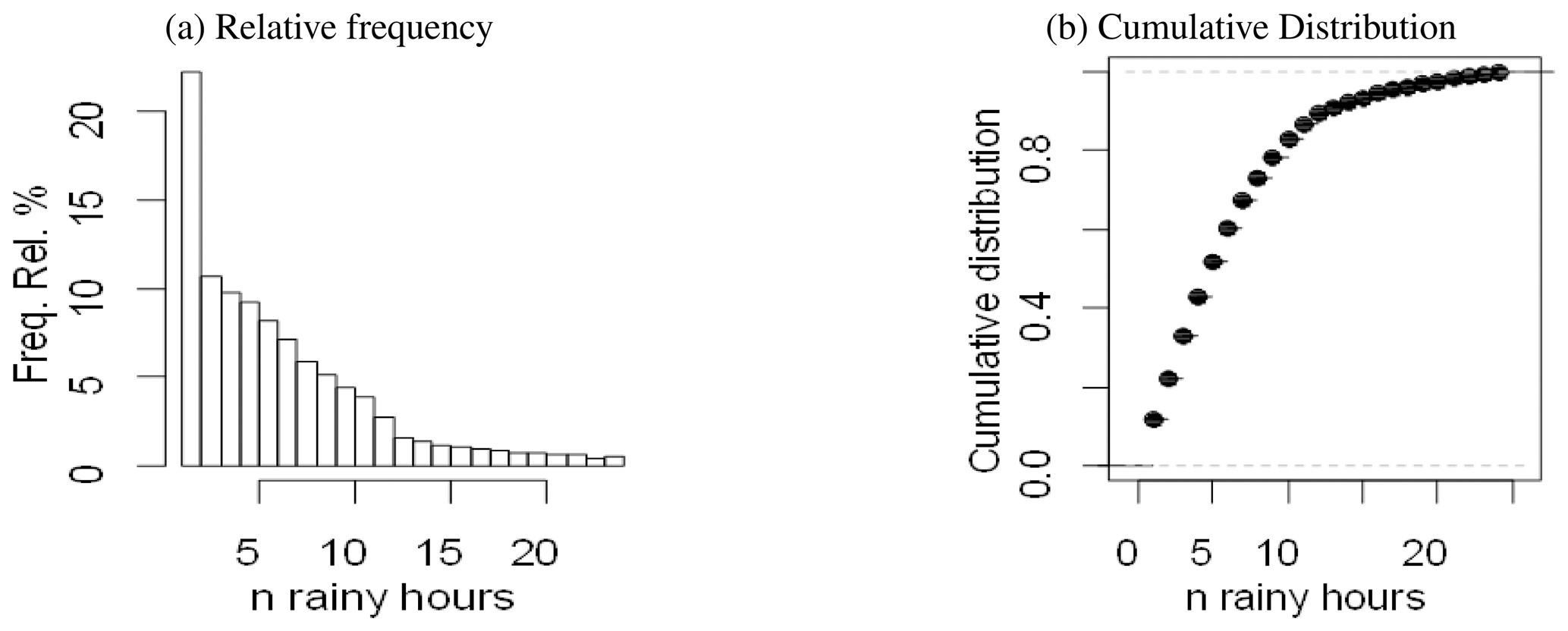
Figure A1Distribution of daily rainy-hour counts from GsMap global hourly data for 2000–2014. (a) Relative frequencies. (b) Cumulative probability.
A5 Pedotransfer functions
From the models tested (Table 2), the equations from Balland et al. (2008), which use the largest dataset and nonlinear formulations, outperformed the other models with the explained variance exceeding 60 % for permanent wilting point (θ1500), field capacity (θ33), and saturation (θsat) (Fig. A2).
The PTFs for computing Ksat showed poor performances for all the models, and most of the measurements seem to cluster around 0 to 50 mm h−1, which is only captured by the Cosby et al. (1984) model. Overall, the explained variance of all the models did not reach 10 % (Fig. A3). Here, Ksat values exceeding 526 mm h−1 were considered to be outliers (percentile 90 %) and excluded from the analysis; similar maximum values were presented by Van Looy et al. (2017).
Ksat estimated by the Saxton and Rawls (2006) PTF was the best-performing model; however, it leads to unrealistic values when the drainable porosity (θsat−θ33) is relatively high. So, a simple exponential saturating curve was adopted here, which yields similar estimations to Saxton and Rawls (2006) at the lower end of the drainable porosity but it flattens at a fitted Ksat maximum of 623 mm h−1.
Furthermore, to improve these estimations, the equations from Balland et al. (2008) (Eqs. A25a, A25b, A25c, A25d) were optimized using the full dataset employed for this evaluation, resulting in the parameters detailed in Table A1.
Here, θ1500 is the wilting point (water held at 1500 kPa), θ33 is the field capacity (water held at 33 kPa), θsat is saturation, Ksat is the saturated hydraulic conductivity, and SAND, CLAY ,and SOM refer to sand, clay, and organic matter contents (%). a, b, and c are constants with the subscripts referring to wilting point, field capacity, or hydraulic saturated conductivity, respectively; ρb is the bulk density, and ρp is the particle density, calculated as follows (Balland et al., 2008):
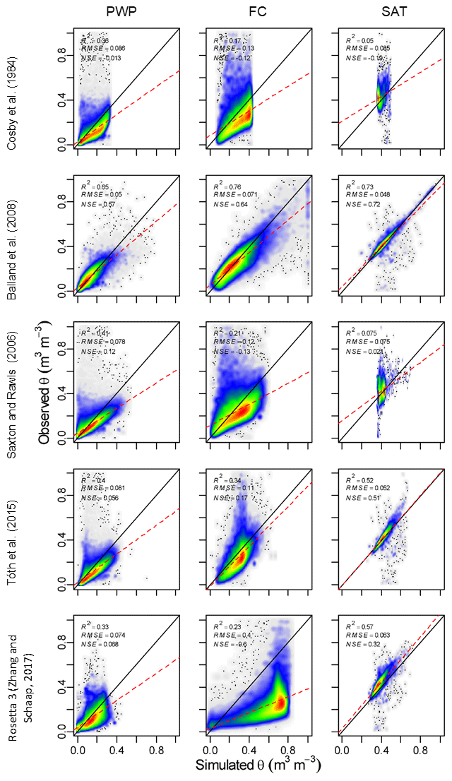
Figure A2Evaluation of different pedotransfer functions to estimate θ1500, θ33, and θsat for n=68 567. The color scale represents the plotted point density, where blue indicates lower densities and red indicates higher densities.
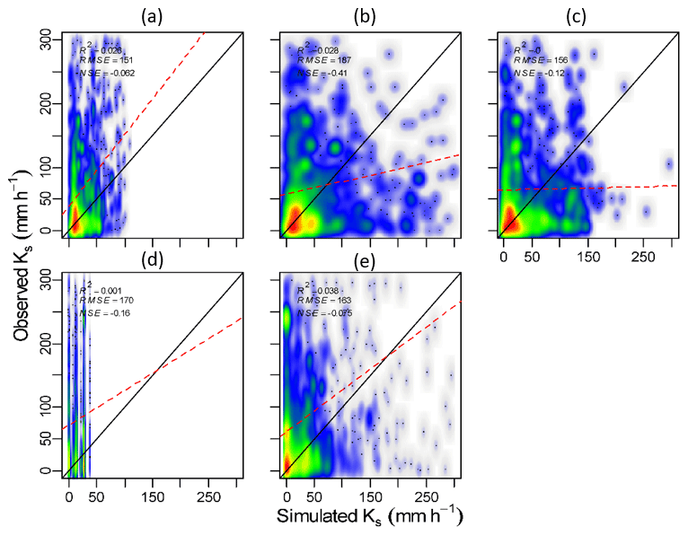
Figure A3Evaluation of different pedotransfer functions to estimate Ksat. The color scale represents the plotted point density, where blue indicates lower densities and red indicates higher densities. (a) Cosby et al. (1984). (b) Balland et al. (2008). (c) Saxton and Rawls (2006). (d) Tóth et al. (2015). (e) Rosetta 3 (Zhang and Schaap, 2017).
Table A1Updated parameters for the Balland et al. (2008) PTFs.
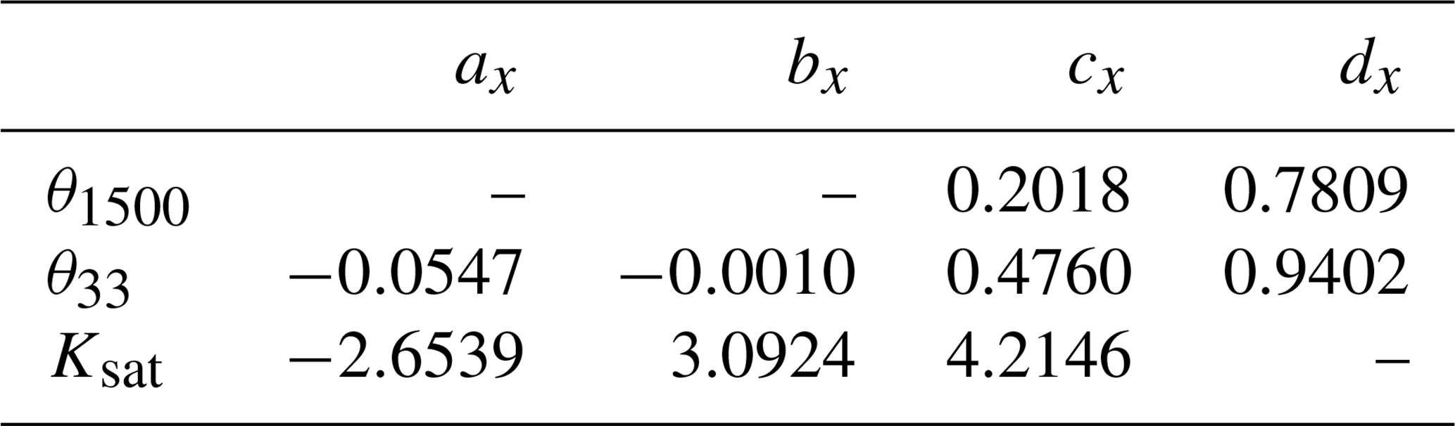
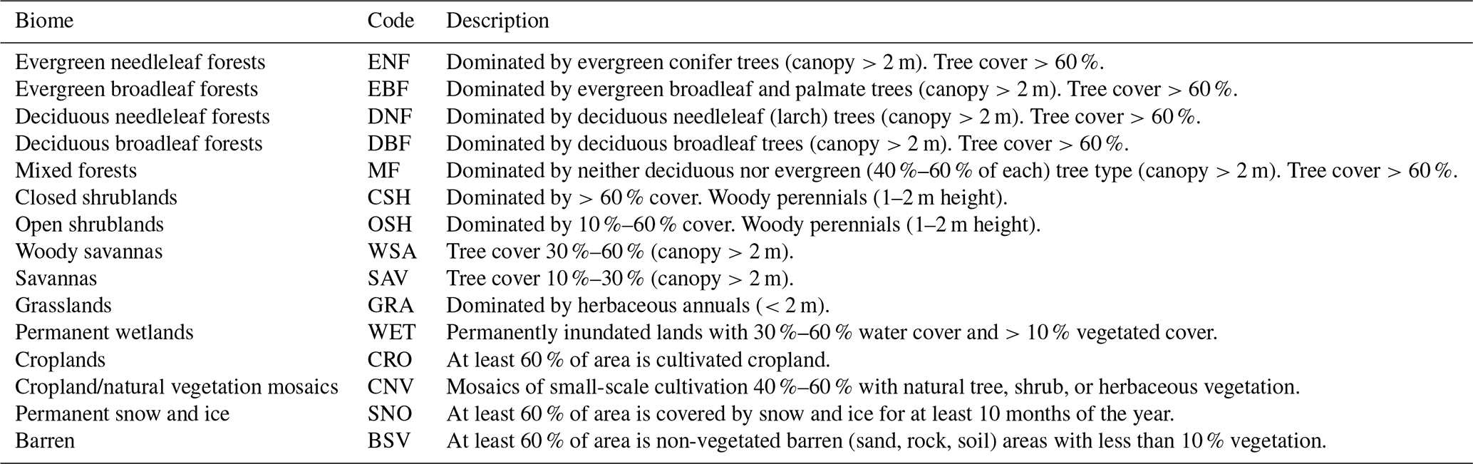
Table A3Köppen–Geiger climate zones after Beck et al. (2018). Tcold is the air temperature of the coldest month (°C); Thot is the air temperature of the warmest month (°C); Tmon10 is the number of months with air temperature >10 °C (unitless); Pdry is the precipitation in the driest month (mm per month); Psdry is the precipitation in the driest month in summer (mm per month); Pwdry is precipitation in the driest month in winter (mm per month); Pswet is precipitation in the wettest month in summer (mm per month); Pwwet is precipitation in the wettest month in winter (mm per month). if >70 % of precipitation falls in winter, and if >70 % of precipitation falls in summer; otherwise, .
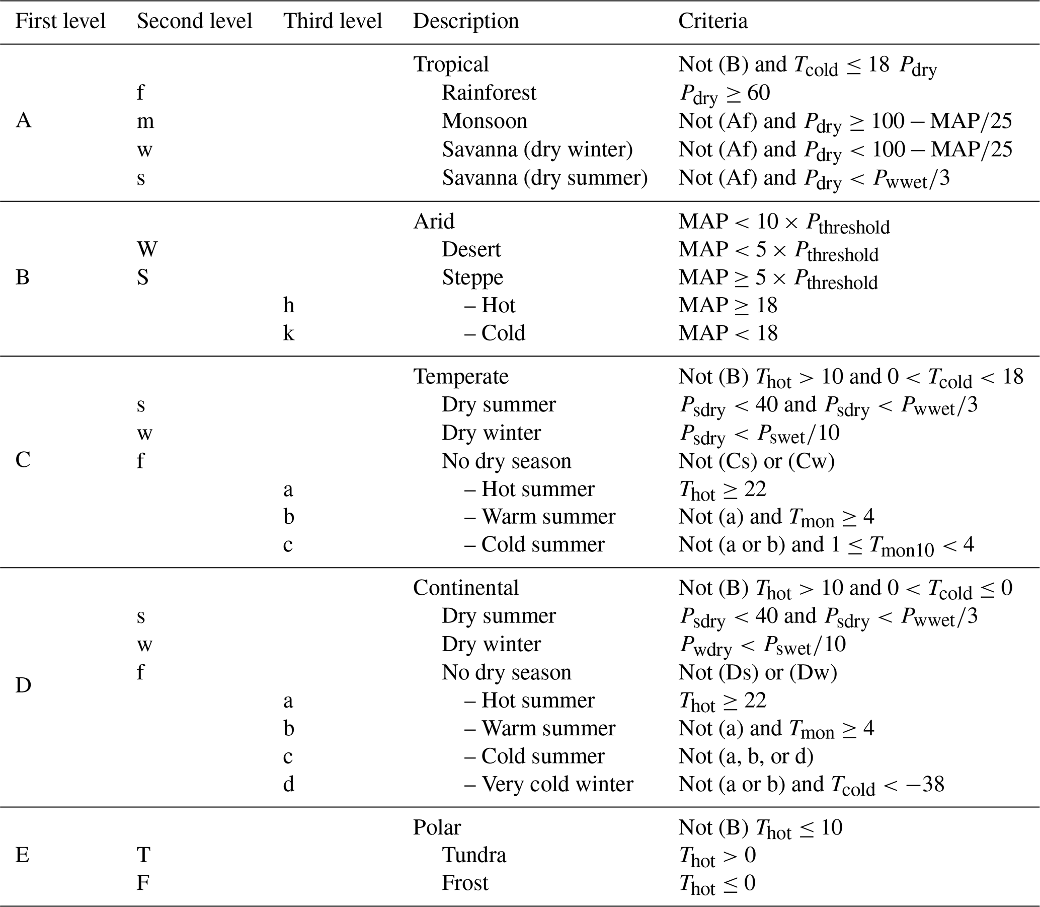
Table A4Eddy covariance stations used in the performance evaluation. Lat. is latitude (°), Long. is longitude (°), and Net. is the network; here FLX, EUR, and AME stand for FLUXNET, EuropeFlux, and AmeriFlux, respectively. Climate refers to the Köppen–Geiger climate zone and “biome” as defined by the IGBP (Table A2) (Friedl et al., 2019). Elev. is the elevation in m a.s.l., Slop. and Asp. are the slope (°) and aspect (°), respectively, and Au. is the upslope draining area (km2).
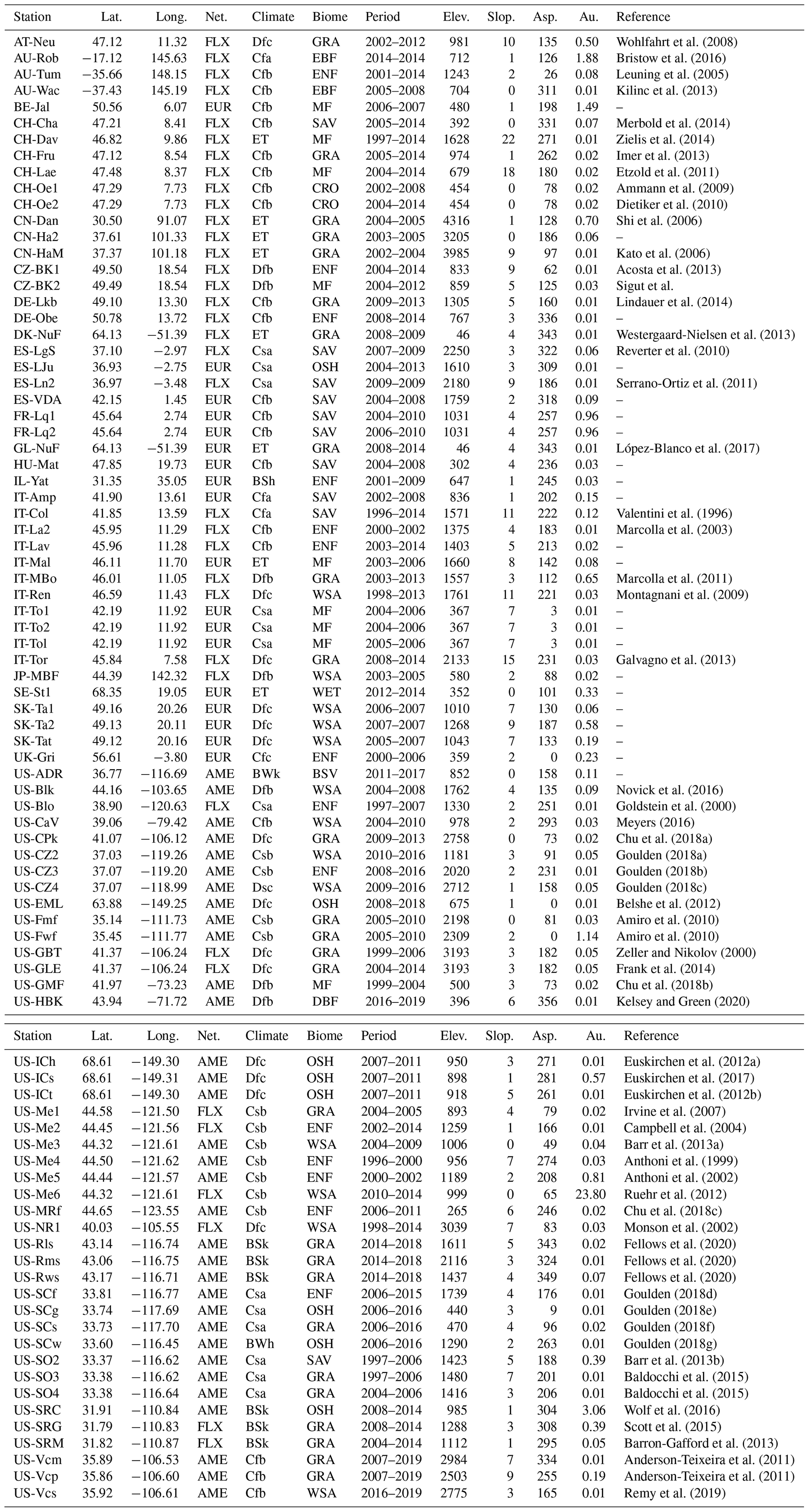
Table A5SNOTEL stations used in the performance evaluation. Lat. is latitude (°), Long. is longitude (°), and Climate refers to the Köppen–Geiger climate zone with “biome” as defined by the IGBP (Table A2) (Friedl et al., 2019). Elev. is the elevation in m a.s.l., Slop. and Asp. are the slope (°) and aspect (°), respectively, Au. is the upslope draining area (km2), and depth is the maximum depth of the soil profile (m) where the soil moisture was measured.
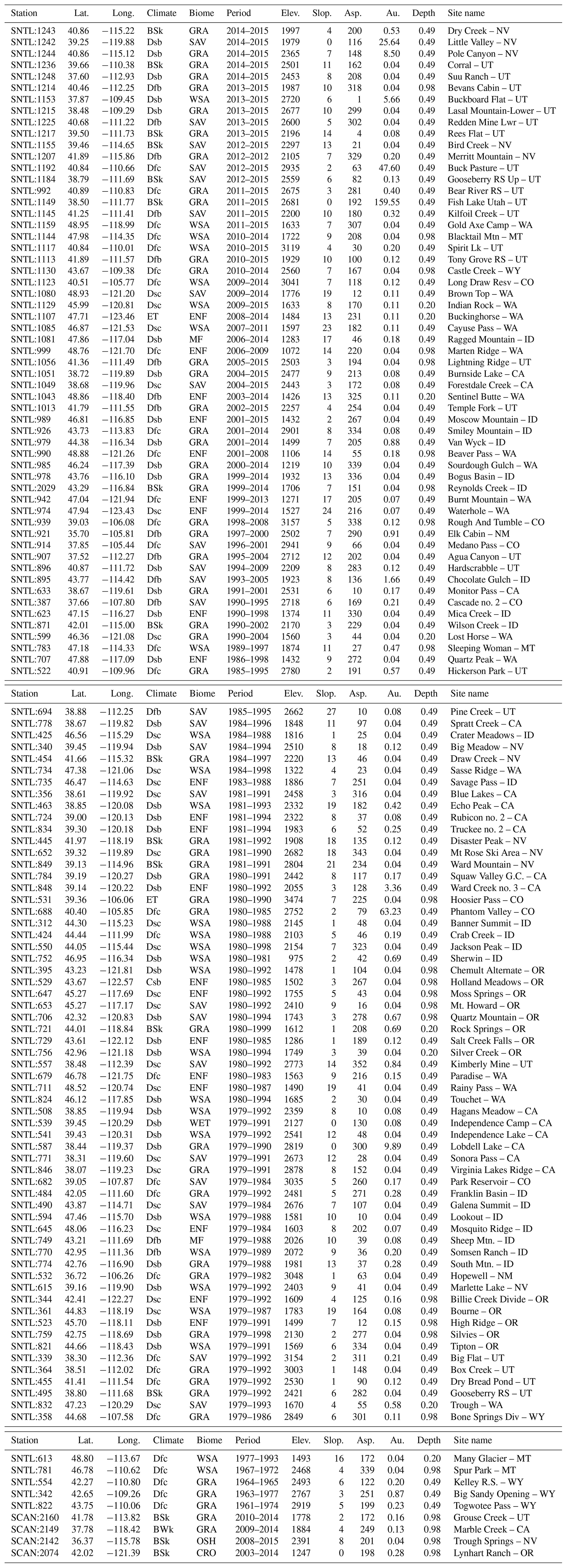
Table A6GSIM hydrometric stations used in the streamflow performance evaluation. Lat. is latitude (°), Long. is longitude (°), Climate refers to the three largest Köppen–Geiger climate zones in the watershed, and “biome” refers to the three largest biomes in the watershed, as defined by the IGBP (Table A2) (Friedl et al., 2019). Elev. is the elevation range in m a.s.l. Area is the watershed area (km2), and “river” lists the river name and country.

The equations and methods presented in this chapter were coded in C++ to improve the speed of the computation. Aiming for replicability, the codes were wrapped in an open-source R package called “rsplash” available on Zenodo at https://doi.org/10.5281/zenodo.10047627, (Sandoval, 2023) and on GitHub at https://github.com/dsval/rsplash (last access: 7 August 2023). The algorithms can either run at site scale or be spatially distributed on a grid. The package is coded to automatically exploit parallel computing capabilities when required. A companion R package called “splashTools” was created (https://github.com/dsval/splashTools, last access: 26 January 2021; DOI: https://doi.org/10.5281/zenodo.11220559, Sandoval, 2024) including all the wrappers and original code for downloading and pre-processing forcing and soil data from the US Natural Resources Conservation Services, SoilGrids, FLUXNET, and other cited sources. All the datasets used in this research are open-access and available through their respective sources cited in the text (see Sect. 5, “Methods: input data”).
DS: conceptualization, software, and writing (original draft preparation). ICP: writing (review and editing), supervision. RLBN: writing (review and editing).
The contact author has declared that none of the authors has any competing interests.
Publisher's note: Copernicus Publications remains neutral with regard to jurisdictional claims made in the text, published maps, institutional affiliations, or any other geographical representation in this paper. While Copernicus Publications makes every effort to include appropriate place names, the final responsibility lies with the authors.
This research is a contribution to the Land Ecosystem Models based On New Theory, obseRvations and ExperimEnts (LEMONTREE) project funded through the generosity of Eric and Wendy Schmidt by recommendation of the Schmidt Futures program.
This research has been supported by the European Research Council H2020 (grant no. 787203) and the Ecuadorian Secretaría de Educación Superior, Ciencia, Tecnología e Innovación (grant no. CZ02-000388-2017).
This paper was edited by Tomomichi Kato and reviewed by two anonymous referees.
Abatzoglou, J. T.: Development of gridded surface meteorological data for ecological applications and modelling, Int. J. Climatol., 33, 121–131, https://doi.org/10.1002/joc.3413, 2013. a
Abatzoglou, J. T., Dobrowski, S. Z., Parks, S. A., and Hegewisch, K. C.: TerraClimate, a high-resolution global dataset of monthly climate and climatic water balance from 1958–2015, Scientific Data, 5, 170191, https://doi.org/10.1038/sdata.2017.191, 2018. a
Acosta, M., Pavelka, M., Montagnani, L., Kutsch, W., Lindroth, A., Juszczak, R., and Janouš, D.: Soil surface CO2 efflux measurements in Norway spruce forests: Comparison between four different sites across Europe – from boreal to alpine forest, Geoderma, 192, 295–303, https://doi.org/10.1016/j.geoderma.2012.08.027, 2013. a
Allen, R. G.: Assessing Integrity of Weather Data for Reference Evapotranspiration Estimation, J. Irrig. Drain. E., 122, 97–106, https://doi.org/10.1061/(ASCE)0733-9437(1996)122:2(97), 1996. a
Allen, R. G., Trezza, R., and Tasumi, M.: Analytical integrated functions for daily solar radiation on slopes, Agr. Forest Meteorol., 139, 55–73, https://doi.org/10.1016/j.agrformet.2006.05.012, 2006. a, b
Amatulli, G., Domisch, S., Tuanmu, M.-N., Parmentier, B., Ranipeta, A., Malczyk, J., and Jetz, W.: A suite of global, cross-scale topographic variables for environmental and biodiversity modeling, Scientific Data, 5, 180040, https://doi.org/10.1038/sdata.2018.40, 2018. a
Amiro, B. D., Barr, A. G., Barr, J. G., Black, T. A., Bracho, R., Brown, M., Chen, J., Clark, K. L., Davis, K. J., Desai, A. R., Dore, S., Engel, V., Fuentes, J. D., Goldstein, A. H., Goulden, M. L., Kolb, T. E., Lavigne, M. B., Law, B. E., Margolis, H. A., Martin, T., McCaughey, J. H., Misson, L., Montes-Helu, M., Noormets, A., Randerson, J. T., Starr, G., and Xiao, J.: Ecosystem carbon dioxide fluxes after disturbance in forests of North America, J. Geophys. Res., 115, G00K02, https://doi.org/10.1029/2010JG001390, 2010. a, b
Ammann, C., Spirig, C., Leifeld, J., and Neftel, A.: Assessment of the nitrogen and carbon budget of two managed temperate grassland fields, Agr. Ecosyst. Environ., 133, 150–162, https://doi.org/10.1016/j.agee.2009.05.006, 2009. a
Anderson-Teixeira, K. J., Delong, J., Fox, A., Brese, D. A., and Litvak, M.: Differential responses of production and respiration to temperature and moisture drive the carbon balance across a climatic gradient in New Mexico, Glob. Change Biol., 17, 410–424, https://doi.org/10.1111/j.1365-2486.2010.02269.x, 2011. a, b
Anthoni, P. M., Law, B. E., and Unsworth, M. H.: Carbon and water vapor exchange of an open-canopied ponderosa pine ecosystem, Agr. Forest Meteorol., 95, 151–168, https://doi.org/10.1016/S0168-1923(99)00029-5, 1999. a
Anthoni, P. M., Unsworth, M. H., Law, B. E., Irvine, J., Baldocchi, D. D., Tuyl, S. V., and Moore, D.: Seasonal differences in carbon and water vapor exchange in young and old-growth ponderosa pine ecosystems, Agr. Forest Meteorol., 111, 203–222, https://doi.org/10.1016/S0168-1923(02)00021-7, 2002. a
Assouline, S.: Infiltration into soils: Conceptual approaches and solutions, Water Resour. Res., 49, 1755–1772, https://doi.org/10.1002/wrcr.20155, 2013. a, b
Bai, J., Zhang, G., Zhao, Q., Lu, Q., Jia, J., Cui, B., and Liu, X.: Depth-distribution patterns and control of soil organic carbon in coastal salt marshes with different plant covers, Scientific Reports, 6, 34835, https://doi.org/10.1038/srep34835, 2016. a
Baldocchi, D., Sturtevant, C., and Contributors, F.: Does day and night sampling reduce spurious correlation between canopy photosynthesis and ecosystem respiration?, Agr. Forest Meteorol., 207, 117–126, https://doi.org/10.1016/j.agrformet.2015.03.010, 2015. a, b
Balland, V., Pollacco, J. A., and Arp, P. A.: Modeling soil hydraulic properties for a wide range of soil conditions, Ecol. Model., 219, 300–316, https://doi.org/10.1016/j.ecolmodel.2008.07.009, 2008. a, b, c, d, e, f, g, h
Barr, A., Richardson, A., Hollinger, D., Papale, D., Arain, M., Black, T., Bohrer, G., Dragoni, D., Fischer, M., Gu, L., Law, B., Margolis, H., McCaughey, J., Munger, J., Oechel, W., and Schaeffer, K.: Use of change-point detection for friction–velocity threshold evaluation in eddy-covariance studies, Agr. Forest Meteorol., 171-172, 31–45, https://doi.org/10.1016/j.agrformet.2012.11.023, 2013a. a
Barr, A., Richardson, A., Hollinger, D., Papale, D., Arain, M., Black, T., Bohrer, G., Dragoni, D., Fischer, M., Gu, L., Law, B., Margolis, H., McCaughey, J., Munger, J., Oechel, W., and Schaeffer, K.: Use of change-point detection for friction–velocity threshold evaluation in eddy-covariance studies, Agr. Forest Meteorol., 171-172, 31–45, https://doi.org/10.1016/j.agrformet.2012.11.023, 2013b. a
Barron-Gafford, G. A., Scott, R. L., Jenerette, G. D., Hamerlynck, E. P., and Huxman, T. E.: Landscape and environmental controls over leaf and ecosystem carbon dioxide fluxes under woody plant expansion, J. Ecol., 101, 1471–1483, https://doi.org/10.1111/1365-2745.12161, 2013. a
Barry, R. G.: The parameterization of surface albedo for sea ice and its snow cover, Prog. Phys. Geog., 20, 63–79, 1996. a, b
Barry, R. G.: Mountain Weather and Climate, Cambridge University Press, 3rd edn., ISBN 9780521862950, 2008. a, b, c, d
Bastiaanssen, W., Menenti, M., Feddes, R., and Holtslag, A.: A remote sensing surface energy balance algorithm for land (SEBAL). 1. Formulation, J. Hydrol., 212–213, 198–212, https://doi.org/10.1016/S0022-1694(98)00253-4, 1998a. a, b
Bastiaanssen, W., Pelgrum, H., Wang, J., Ma, Y., Moreno, J., Roerink, G., and van der Wal, T.: A remote sensing surface energy balance algorithm for land (SEBAL). 2. Validation, J. Hydrol., 212–213, 213–229, https://doi.org/10.1016/S0022-1694(98)00254-6, 1998b. a
Batjes, N. H., Ribeiro, E., and van Oostrum, A.: Standardised soil profile data to support global mapping and modelling (WoSIS snapshot 2019), Earth Syst. Sci. Data, 12, 299–320, https://doi.org/10.5194/essd-12-299-2020, 2020. a
Beck, H. E., Zimmermann, N. E., McVicar, T. R., Vergopolan, N., Berg, A., and Wood, E. F.: Present and future Köppen-Geiger climate classification maps at 1-km resolution, Scientific Data, 5, 180214, https://doi.org/10.1038/sdata.2018.214, 2018. a, b
Beck, H. E., Wood, E. F., Pan, M., Fisher, C. K., Miralles, D. G., van Dijk, A. I. J. M., McVicar, T. R., and Adler, R. F.: MSWEP V2 Global 3-Hourly 0.1° Precipitation: Methodology and Quantitative Assessment, B. Am. Meteorol. Soc., 100, 473–500, https://doi.org/10.1175/BAMS-D-17-0138.1, 2019. a
Beldring, S., Gottschalk, L., Seibert, J., and Tallaksen, L.: Distribution of soil moisture and groundwater levels at patch and catchment scales, Agr. Forest Meteorol., 98–99, 305–324, https://doi.org/10.1016/S0168-1923(99)00103-3, 1999. a
Belshe, E. F., Schuur, E. A. G., Bolker, B. M., and Bracho, R.: Incorporating spatial heterogeneity created by permafrost thaw into a landscape carbon estimate, J. Geophys. Res.-Biogeo., 117, G01026, https://doi.org/10.1029/2011JG001836, 2012. a
Bergström, S.: The HBV model, in: Computer Models of Watershed Hydrology, edited by: Singh, V., Water Resources Publications, Highlands Ranch, CO, 443–476, ISBN 0918334918, 1995. a
Beven, K. J. and Kirby, M. J.: A physically based, variable contributing area model of basin hydrology, Hydrol. Sci. B., 24, 43–69, https://doi.org/10.1080/02626667909491834, 1979. a
Bristow, M., Hutley, L. B., Beringer, J., Livesley, S. J., Edwards, A. C., and Arndt, S. K.: Quantifying the relative importance of greenhouse gas emissions from current and future savanna land use change across northern Australia, Biogeosciences, 13, 6285–6303, https://doi.org/10.5194/bg-13-6285-2016, 2016. a
Brooks, R. H. and Corey, A. T.: Hydraulic Properties of Porous Media, Transactions of the ASAE, 7, 0026–0028, https://doi.org/10.13031/2013.40684, 1964. a, b, c
Buytaert, W., De Bièvre, B., Wyseure, G., and Deckers, J.: The use of the linear reservoir concept to quantify the impact of changes in land use on the hydrology of catchments in the Andes, Hydrol. Earth Syst. Sci., 8, 108–114, https://doi.org/10.5194/hess-8-108-2004, 2004. a
Campbell, G. S. and Norman, J. M.: An Introduction to Environmental Biophysics, Springer New York, New York, NY, ISBN 978-0-387-94937-6, https://doi.org/10.1007/978-1-4612-1626-1, 1998. a, b, c, d, e
Campbell, J. L., Sun, O. J., and Law, B. E.: Disturbance and net ecosystem production across three climatically distinct forest landscapes, Global Biogeochem. Cy., 18, GB4017, https://doi.org/10.1029/2004GB002236, 2004. a
Chapin, F. S. I., Matson, P. A., and Vitousek, P. M.: Principles of Terrestrial Ecosystem Ecology, Springer New York, New York, NY, ISBN 978-1-4419-9503-2, https://doi.org/10.1007/978-1-4419-9504-9, 2011. a, b
Chen, A., Li, W., Li, W., and Liu, X.: An observational study of snow aging and the seasonal variation of snow albedo by using data from Col de Porte, France, Chinese Sci. Bull., 59, 4881–4889, https://doi.org/10.1007/s11434-014-0429-9, 2014. a
Chu, H., Baldocchi, D. D., Poindexter, C., Abraha, M., Desai, A. R., Bohrer, G., Arain, M. A., Griffis, T., Blanken, P. D., O'Halloran, T. L., Thomas, R. Q., Zhang, Q., Burns, S. P., Frank, J. M., Christian, D., Brown, S., Black, T. A., Gough, C. M., Law, B. E., Lee, X., Chen, J., Reed, D. E., Massman, W. J., Clark, K., Hatfield, J., Prueger, J., Bracho, R., Baker, J. M., and Martin, T. A.: Temporal Dynamics of Aerodynamic Canopy Height Derived From Eddy Covariance Momentum Flux Data Across North American Flux Networks, Geophys. Res. Lett., 45, 9275–9287, https://doi.org/10.1029/2018GL079306, 2018a. a
Chu, H., Baldocchi, D. D., Poindexter, C., Abraha, M., Desai, A. R., Bohrer, G., Arain, M. A., Griffis, T., Blanken, P. D., O'Halloran, T. L., Thomas, R. Q., Zhang, Q., Burns, S. P., Frank, J. M., Christian, D., Brown, S., Black, T. A., Gough, C. M., Law, B. E., Lee, X., Chen, J., Reed, D. E., Massman, W. J., Clark, K., Hatfield, J., Prueger, J., Bracho, R., Baker, J. M., and Martin, T. A.: Temporal Dynamics of Aerodynamic Canopy Height Derived From Eddy Covariance Momentum Flux Data Across North American Flux Networks, Geophys. Res. Lett., 45, 9275–9287, https://doi.org/10.1029/2018GL079306, 2018b. a
Chu, H., Baldocchi, D. D., Poindexter, C., Abraha, M., Desai, A. R., Bohrer, G., Arain, M. A., Griffis, T., Blanken, P. D., O'Halloran, T. L., Thomas, R. Q., Zhang, Q., Burns, S. P., Frank, J. M., Christian, D., Brown, S., Black, T. A., Gough, C. M., Law, B. E., Lee, X., Chen, J., Reed, D. E., Massman, W. J., Clark, K., Hatfield, J., Prueger, J., Bracho, R., Baker, J. M., and Martin, T. A.: Temporal Dynamics of Aerodynamic Canopy Height Derived From Eddy Covariance Momentum Flux Data Across North American Flux Networks, Geophys. Res. Lett., 45, 9275–9287, https://doi.org/10.1029/2018GL079306, 2018c. a
Clark, M. P., Bierkens, M. F. P., Samaniego, L., Woods, R. A., Uijlenhoet, R., Bennett, K. E., Pauwels, V. R. N., Cai, X., Wood, A. W., and Peters-Lidard, C. D.: The evolution of process-based hydrologic models: historical challenges and the collective quest for physical realism, Hydrol. Earth Syst. Sci., 21, 3427–3440, https://doi.org/10.5194/hess-21-3427-2017, 2017. a, b, c
Corps of Engineers: Summary report of the snow investigations, snow hydrology, Army Engineer Division, Portland, US, https://usace.contentdm.oclc.org/digital/collection/p266001coll1/id/4172/ (last access: 5 May 2021), 1956. a
Correa, A., Ochoa-Tocachi, B. F., Birkel, C., Ochoa-Sánchez, A., Zogheib, C., Tovar, C., and Buytaert, W.: A concerted research effort to advance the hydrological understanding of tropical páramos, Hydrol. Process., 34, 4609–4627, https://doi.org/10.1002/hyp.13904, 2020. a, b
Cosby, B. J., Hornberger, G. M., Clapp, R. B., and Ginn, T. R.: A Statistical Exploration of the Relationships of Soil Moisture Characteristics to the Physical Properties of Soils, Water Resour. Res., 20, 682–690, https://doi.org/10.1029/WR020i006p00682, 1984. a, b, c
Cramer, W. and Prentice, I. C.: Simulation of regional soil moisture deficits on a European scale, Norsk Geogr. Tidsskr., 12, 149–151, https://doi.org/10.1080/00291958808552193, 1988. a
Crespo, P. J., Feyen, J., Buytaert, W., Bücker, A., Breuer, L., Frede, H.-G., and Ramírez, M.: Identifying controls of the rainfall–runoff response of small catchments in the tropical Andes (Ecuador), J. Hydrol., 407, 164–174, https://doi.org/10.1016/j.jhydrol.2011.07.021, 2011. a, b
Davis, T. W., Prentice, I. C., Stocker, B. D., Thomas, R. T., Whitley, R. J., Wang, H., Evans, B. J., Gallego-Sala, A. V., Sykes, M. T., and Cramer, W.: Simple process-led algorithms for simulating habitats (SPLASH v.1.0): robust indices of radiation, evapotranspiration and plant-available moisture, Geosci. Model Dev., 10, 689–708, https://doi.org/10.5194/gmd-10-689-2017, 2017. a, b, c, d, e, f, g, h, i, j, k, l, m, n
Dickinson, R. E., Henderson-Sellers, A., Kennedy, P. J., and Wilson, M. F.: Biosphere-Atmosphere Transfer Scheme (BATS) for the NCAR Community Climate Model, https://doi.org/10.5065/D6668B58, 1986. a
Dietiker, D., Buchmann, N., and Eugster, W.: Testing the ability of the {DNDC} model to predict CO2 and water vapour fluxes of a {S}wiss cropland site, Agr. Ecosyst. Environ., 139, 396–401, https://doi.org/10.1016/j.agee.2010.09.002, 2010. a
Dirmeyer, P. A., Gao, X., Zhao, M., Guo, Z., Oki, T., and Hanasaki, N.: GSWP-2: Multimodel analysis and implications for our perception of the land surface, B. Am. Meteorol. Soc., 87, 1381–1397, https://doi.org/10.1175/BAMS-87-10-1381, 2006. a
Do, H. X., Gudmundsson, L., Leonard, M., and Westra, S.: The Global Streamflow Indices and Metadata Archive (GSIM) – Part 1: The production of a daily streamflow archive and metadata, Earth Syst. Sci. Data, 10, 765–785, https://doi.org/10.5194/essd-10-765-2018, 2018. a
Dunkerley, D.: Identifying individual rain events from pluviograph records: a review with analysis of data from an Australian dryland site, Hydrol. Process., 22, 5024–5036, https://doi.org/10.1002/hyp.7122, 2008. a
Etzold, S., Ruehr, N. K., Zweifel, R., Dobbertin, M., Zingg, A., Pluess, P., Häsler, R., Eugster, W., and Buchmann, N.: The Carbon Balance of Two Contrasting Mountain Forest Ecosystems in {S}witzerland: Similar Annual Trends, but Seasonal Differences, Ecosystems, 14, 1289–1309, https://doi.org/10.1007/s10021-011-9481-3, 2011. a
Euskirchen, E. S., Bret-Harte, M. S., Scott, G. J., Edgar, C., and Shaver, G. R.: Seasonal patterns of carbon dioxide and water fluxes in three representative tundra ecosystems in northern Alaska, Ecosphere, 3, 4, https://doi.org/10.1890/ES11-00202.1, 2012a. a
Euskirchen, E. S., Bret-Harte, M. S., Scott, G. J., Edgar, C., and Shaver, G. R.: Seasonal patterns of carbon dioxide and water fluxes in three representative tundra ecosystems in northern Alaska, Ecosphere, 3, 4, https://doi.org/10.1890/ES11-00202.1, 2012b. a
Euskirchen, E. S., Bret-Harte, M. S., Shaver, G. R., Edgar, C. W., and Romanovsky, V. E.: Long-Term Release of Carbon Dioxide from Arctic Tundra Ecosystems in Alaska, Ecosystems, 20, 960–974, https://doi.org/10.1007/s10021-016-0085-9, 2017. a
Fan, Y., Miguez-Macho, G., Weaver, C. P., Walko, R., and Robock, A.: Incorporating water table dynamics in climate modeling: 1. Water table observations and equilibrium water table simulations, J. Geophys. Res.-Atmos., 112, D10125, https://doi.org/10.1029/2006JD008111, 2007. a, b, c, d, e
Fawcett, T.: An introduction to ROC analysis, Pattern Recogn. Lett., 27, 861–874, https://doi.org/10.1016/j.patrec.2005.10.010, 2006. a
Feddes, R. A. and Raats, P. A.: Parameterizing the soil – water – plant root system, in: Unsaturated-zone Modeling: Progress, Challenges and Applications, edited by: Feddes, R., de Rooij, G., and van Dam, J., Springer Netherlands, https://edepot.wur.nl/35358 (last access: 29 March 2019), 2004. a
Federer, C. A.: Spatial Variation of Net Radiation, Albedo and Surface Temperature of Forests, J. Appl. Meteorol., 7, 789–795, https://doi.org/10.1175/1520-0450(1968)007<0789:SVONRA>2.0.CO;2, 1968. a, b
Federer, C. A.: Transpirational supply and demand: Plant, soil, and atmospheric effects evaluated by simulation, Water Resour. Res., 18, 355–362, https://doi.org/10.1029/WR018i002p00355, 1982. a, b, c, d, e, f
Fellows, A. W., Flerchinger, G. N., Seyfried, M. S., Biederman, J. A., and Lohse, K. A.: Winter CO2 Efflux From Sagebrush Shrublands Distributed Across the Rain‐to‐Snow Transition Zone, J. Geophys. Res.-Biogeo., 125, e2019JG005325, https://doi.org/10.1029/2019JG005325, 2020. a, b, c
Frank, J. M., Massman, W. J., Ewers, B. E., Huckaby, L. S., and Negrõn, J. F.: Ecosystem fluxes are explained by hydraulically limited gas exchange during tree mortality from spruce bark beetles, J. Geophys. Res.-Biogeo., 119, 1195–1215, https://doi.org/10.1002/2013JG002597, 2014. a
Friedl, M., Gray, J., and Sulla-Menashe, D.: MCD12Q2 MODIS/Terra+Aqua Land Cover Dynamics Yearly L3 Global 500m SIN Grid V006, NASA EOSDIS Land Processes Distributed Active Archive Center [data set], https://doi.org/10.5067/MODIS/MCD12Q2.006, 2019. a, b, c, d
Gallego-Sala, A. V. and Prentice, I. C.: Blanket peat biome endangered by climate change, Nat. Clim. Change, 3, 152–155, https://doi.org/10.1038/nclimate1672, 2012. a
Galvagno, M., Wohlfahrt, G., Cremonese, E., Rossini, M., Colombo, R., Filippa, G., Julitta, T., Manca, G., Siniscalco, C., Morra Di Cella, U., and Migliavacca, M.: Phenology and carbon dioxide source/sink strength of a subalpine grassland in response to an exceptionally short snow season, Environ. Res. Lett., 8, 25008, https://doi.org/10.1088/1748-9326/8/2/025008, 2013. a
Gao, H., Tang, Q., Shi, X., Zhu, C., Bohn, T., Su, F., Sheffield, J., Pan, M., Lettenmaier, D., and Wood, E. F.: Water budget record from Variable Infiltration Capacity (VIC) model. Algorithm Theoretical Basis Document, Version 1.2, in: Algorithm theoretical basis document for terrestrial water cycle data records, Department of Civil and Environmental Engineering, University of Washington, 120–173, https://eprints.lancs.ac.uk/id/eprint/89407/1/Gao_et_al_VIC_2014.pdf (last access: 21 June 2021), 2009. a
Goldstein, A. H., Hultman, N. E., Fracheboud, J. M., Bauer, M. R., Panek, J. A., Xu, M., Qi, Y., Guenther, A. B., and Baugh, W.: Effects of climate variability on the carbon dioxide, water, and sensible heat fluxes above a ponderosa pine plantation in the Sierra Nevada (CA), Agr. Forest Meteorol., 101, 113–129, https://doi.org/10.1016/S0168-1923(99)00168-9, 2000. a
Goulden, M.: AmeriFlux US-CZ2 Sierra Critical Zone, Sierra Transect, Ponderosa Pine Forest, Soaproot Saddle, AmeriFlux [data set], https://doi.org/10.17190/AMF/1419510, 2018a. a
Goulden, M.: AmeriFlux US-CZ3 Sierra Critical Zone, Sierra Transect, Sierran Mixed Conifer, P301, AmeriFlux [data set], https://doi.org/10.17190/AMF/1419512, 2018b. a
Goulden, M.: AmeriFlux US-CZ4 Sierra Critical Zone, Sierra Transect, Subalpine Forest, Shorthair, AmeriFlux [data set], https://doi.org/10.17190/AMF/1419511, 2018c. a
Goulden, M.: AmeriFlux US-SCf Southern California Climate Gradient – Oak/Pine Forest, AmeriFlux [data set], https://doi.org/10.17190/AMF/1419503, 2018d. a
Goulden, M.: AmeriFlux US-SCg Southern California Climate Gradient – Grassland, AmeriFlux [data set], https://doi.org/10.17190/AMF/1419502, 2018e. a
Goulden, M.: AmeriFlux US-SCs Southern California Climate Gradient – Coastal Sage, AmeriFlux [data set], https://doi.org/10.17190/AMF/1419501, 2018f. a
Goulden, M.: AmeriFlux US-SCw Southern California Climate Gradient – Pinyon/Juniper Woodland, AmeriFlux [data set], https://doi.org/10.17190/AMF/1419504, 2018g. a
Grayson, R. B. and Blöschl, G.: Spatial patterns in catchment hydrology: observations and modelling, Cambridge University Press, ISBN 9780521633161, 2000. a, b, c, d
Guo, X., Zha, T., Jia, X., Wu, B., Feng, W., Xie, J., Gong, J., Zhang, Y., and Peltola, H.: Dynamics of Dew in a Cold Desert-Shrub Ecosystem and Its Abiotic Controls, Atmosphere, 7, 32, https://doi.org/10.3390/atmos7030032, 2016. a
Gupta, H. V. and Kling, H.: On typical range, sensitivity, and normalization of Mean Squared Error and Nash-Sutcliffe Efficiency type metrics, Water Resour. Res., 47, 2–4, https://doi.org/10.1029/2011WR010962, 2011. a
Gurtz, J., Zappa, M., Jasper, K., Lang, H., Verbunt, M., Badoux, A., and Vitvar, T.: A comparative study in modelling runoff and its components in two mountainous catchments, Hydrol. Process., 17, 297–311, https://doi.org/10.1002/hyp.1125, 2003. a
Hall, D. K., Salomonson, V. V., and Riggs, G. A.: MODIS/Terra Snow Cover Daily L3 Global 500m Grid. Version 6, NASA National Snow and Ice Data Center Distributed Active Archive Center [data set], https://doi.org/10.5067/MODIS/MOD10A1.006, 2016. a
Harder, P. and Pomeroy, J. W.: Hydrological model uncertainty due to precipitation-phase partitioning methods, Hydrol. Process., 28, 4311–4327, https://doi.org/10.1002/hyp.10214, 2014. a
Harrison, S. P., Prentice, I. C., Barboni, D., Kohfeld, K. E., Ni, J., and Sutra, J.-P.: Ecophysiological and bioclimatic foundations for a global plant functional classification, J. Veg. Sci., 21, 300–317, https://doi.org/10.1111/j.1654-1103.2009.01144.x, 2010. a
Harrison, S. P., Cramer, W., Franklin, O., Prentice, I. C., Wang, H., Brännström, Å., Boer, H., Dieckmann, U., Joshi, J., Keenan, T. F., Lavergne, A., Manzoni, S., Mengoli, G., Morfopoulos, C., Peñuelas, J., Pietsch, S., Rebel, K. T., Ryu, Y., Smith, N. G., Stocker, B. D., and Wright, I. J.: Eco‐evolutionary optimality as a means to improve vegetation and land‐surface models, New Phytol., 231, 2125–2141, https://doi.org/10.1111/nph.17558, 2021. a
Hengl, T., Mendes de Jesus, J., Heuvelink, G. B. M., Ruiperez Gonzalez, M., Kilibarda, M., Blagotić, A., Shangguan, W., Wright, M. N., Geng, X., Bauer-Marschallinger, B., Guevara, M. A., Vargas, R., MacMillan, R. A., Batjes, N. H., Leenaars, J. G. B., Ribeiro, E., Wheeler, I., Mantel, S., and Kempen, B.: SoilGrids250m: Global gridded soil information based on machine learning, PLOS ONE, 12, e0169748, https://doi.org/10.1371/journal.pone.0169748, 2017. a, b
Hilberts, A. G. J., Troch, P. A., and Paniconi, C.: Storage-dependent drainable porosity for complex hillslopes, Water Resour. Res., 41, W06001, https://doi.org/10.1029/2004WR003725, 2005. a, b, c
Hillel, D.: Environmental Soil Physics: Fundamentals, Applications, and Environmental Considerations, Academic Press, ISBN 9780123485250, 1998. a
Hino, M., Odaka, Y., Nadaoka, K., and Sato, A.: Effect of initial soil moisture content on the vertical infiltration process – A guide to the problem of runoff-ratio and loss, J. Hydrol., 102, 267–284, https://doi.org/10.1016/0022-1694(88)90102-3, 1988. a
Hirschi, M., Michel, D., Lehner, I., and Seneviratne, S. I.: A site-level comparison of lysimeter and eddy covariance flux measurements of evapotranspiration, Hydrol. Earth Syst. Sci., 21, 1809–1825, https://doi.org/10.5194/hess-21-1809-2017, 2017. a
Hobley, E. U. and Wilson, B.: The depth distribution of organic carbon in the soils of eastern Australia, Ecosphere, 7, e01214, https://doi.org/10.1002/ecs2.1214, 2016. a
IFAS: Florida Soil Characterization Retrieval System, https://web.archive.org/web/20210415035753/https://soils.ifas.ufl.edu/flsoils/databaseintro.asp (last access: 25 August 2021), 2007. a
Imer, D., Merbold, L., Eugster, W., and Buchmann, N.: Temporal and spatial variations of soil CO2, CH4 and N2O fluxes at three differently managed grasslands, Biogeosciences, 10, 5931–5945, https://doi.org/10.5194/bg-10-5931-2013, 2013. a
Irvine, J., Law, B. E., and Hibbard, K. A.: Postfire carbon pools and fluxes in semiarid ponderosa pine in Central Oregon, Glob. Change Biol., 13, 1748–1760, https://doi.org/10.1111/j.1365-2486.2007.01368.x, 2007. a
Jarvis, A., Reuter, H., Nelson, A., and Guevara, E.: Hole-filled SRTM for the globe Version 4, available from the CGIAR-CSI SRTM 90m Database, http://srtm.csi.cgiar.org (last access: 25 August 2021), 2008. a
Jennings, K. S., Winchell, T. S., Livneh, B., and Molotch, N. P.: Spatial variation of the rain-snow temperature threshold across the Northern Hemisphere, Nat. Commun., 9, 1148, https://doi.org/10.1038/s41467-018-03629-7, 2018. a, b, c, d
Jones, H. G.: Plants and Microclimate, Cambridge University Press, Cambridge, ISBN 9780511845727, https://doi.org/10.1017/CBO9780511845727, 2013. a
Kao, S.-C., Ashfaq, M., Rastogi, D., Gangrade, S., Uria Martinez, R., Fernandez, A., Konapala, G., Voisin, N., Zhou, T., Xu, W., Gao, H., Zhao, B., and Zhao, G.: The Third Assessment of the Effects of Climate Change on Federal Hydropower, Tech. rep., Oak Ridge National Laboratory (ORNL), Oak Ridge, TN (United States), ISBN 1800553684, https://doi.org/10.2172/1887712, 2022. a
Karger, D. N., Conrad, O., Böhner, J., Kawohl, T., Kreft, H., Soria-Auza, R. W., Zimmermann, N. E., Linder, H. P., and Kessler, M.: Climatologies at high resolution for the earth's land surface areas, Scientific Data, 4, 170122, https://doi.org/10.1038/sdata.2017.122, 2017. a
Kato, T., Tang, Y., Gu, S., Hirota, M., Du, M., Li, Y., and Zhao, X.: Temperature and biomass influences on interannual changes in CO2 exchange in an alpine meadow on the Qinghai-Tibetan Plateau, Glob. Change Biol., 12, 1285–1298, https://doi.org/10.1111/j.1365-2486.2006.01153.x, 2006. a
Kelsey, E. P. S. U. and Green, M. C. W. R. U.: AmeriFlux US-HBK Hubbard Brook Experimental Forest, AmeriFlux [data set], https://doi.org/10.17190/AMF/1634881, 2020. a
Kienzle, S. W.: A new temperature based method to separate rain and snow, Hydrol. Process., 22, 5067–5085, https://doi.org/10.1002/hyp.7131, 2008. a, b, c
Kilinc, M., Beringer, J., Hutley, L. B., Tapper, N. J., and McGuire, D. A.: Carbon and water exchange of the world's tallest angiosperm forest, Agr. Forest Meteorol., 182-183, 215–224, https://doi.org/10.1016/j.agrformet.2013.07.003, 2013. a
Kopp, G. and Lean, J. L.: A new, lower value of total solar irradiance: Evidence and climate significance, Geophys. Res. Lett., 38, L01706, https://doi.org/10.1029/2010GL045777, 2011. a
Körner, C.: Plant ecology at high elevations, Alpine Plant Life, 3rd edn., 1–7, https://doi.org/10.1007/978-3-030-59538-8_1, 2021. a
Körner, C.: Alpine Plant Life, Springer International Publishing, Cham, Switzerland, 3rd edn., ISBN 978-3-030-59537-1, https://doi.org/10.1007/978-3-030-59538-8, 2021. a, b
Kramer, C. and Gleixner, G.: Soil organic matter in soil depth profiles: Distinct carbon preferences of microbial groups during carbon transformation, Soil Biol. Biochem., 40, 425–433, https://doi.org/10.1016/j.soilbio.2007.09.016, 2008. a
Kramer, P. J. and Boyer, J. S.: Water Relations of Plants and Soils, Academic Press, New York, ISBN 9780080924113, 1995. a, b
Ladson, A. R., Brown, R., Neal, B., and Nathan, R.: A standard approach to baseflow separation using the Lyne and Hollick filter, Australasian Journal of Water Resources, 17, 25–34, https://www.tandfonline.com/doi/pdf/10.7158/13241583.2013.11465417 (last access: 23 January 2023), 2013. a
Laipelt, L., Henrique Bloedow Kayser, R., Santos Fleischmann, A., Ruhoff, A., Bastiaanssen, W., Erickson, T. A., and Melton, F.: Long-term monitoring of evapotranspiration using the SEBAL algorithm and Google Earth Engine cloud computing, ISPRS J. Photogramm., 178, 81–96, https://doi.org/10.1016/j.isprsjprs.2021.05.018, 2021. a
Lawrence, D. M., Fisher, R. A., Koven, C. D., Oleson, K. W., Swenson, S. C., Bonan, G., Collier, N., Ghimire, B., van Kampenhout, L., Kennedy, D., Kluzek, E., Lawrence, P. J., Li, F., Li, H., Lombardozzi, D., Riley, W. J., Sacks, W. J., Shi, M., Vertenstein, M., Wieder, W. R., Xu, C., Ali, A. A., Badger, A. M., Bisht, G., van den Broeke, M., Brunke, M. A., Burns, S. P., Buzan, J., Clark, M., Craig, A., Dahlin, K., Drewniak, B., Fisher, J. B., Flanner, M., Fox, A. M., Gentine, P., Hoffman, F., Keppel-Aleks, G., Knox, R., Kumar, S., Lenaerts, J., Leung, L. R., Lipscomb, W. H., Lu, Y., Pandey, A., Pelletier, J. D., Perket, J., Randerson, J. T., Ricciuto, D. M., Sanderson, B. M., Slater, A., Subin, Z. M., Tang, J., Thomas, R. Q., Val Martin, M., and Zeng, X.: The Community Land Model Version 5: Description of New Features, Benchmarking, and Impact of Forcing Uncertainty, J. Adv. Model. Earth Sy., 11, 4245–4287, https://doi.org/10.1029/2018MS001583, 2019. a
Leij, F., Alves, W., van Genuchten, M. T., and Williams, J.: Unsoda Unsaturated Soil Hydraulic Database, UNSODA 1.0 User's Manual, Report EPA/600/R-96/095, Tech. rep., US Environmental Protection Agency, Ada, Oklahoma, https://cfpub.epa.gov/si/si_public_record_report.cfm?Lab=NRMRL&dirEntryId=124868 (last access: 14 June 2019), 1996. a
Leuning, R., Cleugh, H. A., Zegelin, S. J., and Hughes, D.: Carbon and water fluxes over a temperate Eucalyptus forest and a tropical wet/dry savanna in Australia: measurements and comparison with MODIS remote sensing estimates, Agr. Forest Meteorol., 129, 151–173, https://doi.org/10.1016/j.agrformet.2004.12.004, 2005. a
Liang, X. and Xie, Z.: A new surface runoff parameterization with subgrid-scale soil heterogeneity for land surface models, Adv. Water Resour., 24, 1173–1193, https://doi.org/10.1016/S0309-1708(01)00032-X, 2001. a, b
Liang, X., Wood, E. F., and Lettenmaier, D. P.: Surface Soil Moisture Parameterization of the VIC-2L Model: Evaluation and Modifications, Journal of Global and Planetary Change, 13, 195–206, https://doi.org/10.1016/0921-8181(95)00046-1, 1996. a, b
Linacre, E. T.: Estimating the net-radiation flux, Agr. Meteorol., 5, 49–63, https://doi.org/10.1016/0002-1571(68)90022-8, 1968. a, b, c
Lindauer, M., Schmid, H., Grote, R., Mauder, M., Steinbrecher, R., and Wolpert, B.: Net ecosystem exchange over a non-cleared wind-throw-disturbed upland spruce forest–Measurements and simulations, Agr. Forest Meteorol., 197, 219–234, https://doi.org/10.1016/j.agrformet.2014.07.005, 2014. a
Livneh, B., Xia, Y., Mitchell, K. E., Ek, M. B., and Lettenmaier, D. P.: Noah LSM Snow Model Diagnostics and Enhancements, J. Hydrometeorol., 11, 721–738, https://doi.org/10.1175/2009JHM1174.1, 2010. a
López-Blanco, E., Lund, M., Williams, M., Tamstorf, M. P., Westergaard-Nielsen, A., Exbrayat, J.-F., Hansen, B. U., and Christensen, T. R.: Exchange of CO2 in Arctic tundra: impacts of meteorological variations and biological disturbance, Biogeosciences, 14, 4467–4483, https://doi.org/10.5194/bg-14-4467-2017, 2017. a
Kirkham, M. B.: Field Capacity, Wilting Point, Available Water, and the Non-Limiting Water Range, Principles of Soil and Plant Water Relations, 101–115, https://doi.org/10.1016/B978-0-12-420022-7.00010-0, 2005. a
Marcolla, B., Pitacco, A., and Cescatti, A.: Canopy architecture and turbulence structure in a coniferous forest, Bound.-Lay. Meteorol., 108, 39–59, https://doi.org/10.1023/A:1023027709805, 2003. a
Marcolla, B., Cescatti, A., Manca, G., Zorer, R., Cavagna, M., Fiora, A., Gianelle, D., Rodeghiero, M., Sottocornola, M., and Zampedri, R.: Climatic controls and ecosystem responses drive the inter-annual variability of the net ecosystem exchange of an alpine meadow, Agr. Forest Meteorol., 151, 1233–1243, https://doi.org/10.1016/j.agrformet.2011.04.015, 2011. a
Marks, D., Domingo, J., Susong, D., Link, T., and Garen, D.: A spatially distributed energy balance snowmelt model for application in mountain basins, Hydrol. Process., 13, 1935–1959, https://doi.org/10.1002/(SICI)1099-1085(199909)13:12/13<1935::AID-HYP868>3.0.CO;2-C, 1999. a
Mega, T., Ushio, T., Kubota, T., Kachi, M., Aonashi, K., and Shige, S.: Gauge adjusted global satellite mapping of precipitation (GSMaP_Gauge), in: 2014 XXXIth URSI General Assembly and Scientific Symposium (URSI GASS), Beijing, China, 16–23 August 2014, ISBN 978-1-4673-5225-3, https://doi.org/10.1109/URSIGASS.2014.6929683, 2014. a, b
Merbold, L., Eugster, W., Stieger, J., Zahniser, M., Nelson, D., and Buchmann, N.: Greenhouse gas budget (CO2, CH4 and N2O) of intensively managed grassland following restoration, Glob. Change Biol., 20, 1913–1928, https://doi.org/10.1111/gcb.12518, 2014. a
Metselaar, K. and de Jong van Lier, Q.: The Shape of the Transpiration Reduction Function under Plant Water Stress, Vadose Zone J., 6, 124–139, https://doi.org/10.2136/vzj2006.0086, 2007. a, b, c
Meyers, T. N.: AmeriFlux US-CaV Canaan Valley, AmeriFlux [data set], https://doi.org/10.17190/AMF/1246042, 2016. a
Molina-Sanchis, I., Lázaro, R., Arnau-Rosalén, E., and Calvo-Cases, A.: Rainfall timing and runoff: The influence of the criterion for rain event separation, J. Hydrol. Hydromech., 64, 226–236, https://doi.org/10.1515/johh-2016-0024, 2016. a
Monson, R. K., Turnipseed, A. A., Sparks, J. P., Harley, P. C., Scott-Denton, L. E., Sparks, K., and Huxman, T. E.: Carbon sequestration in a high-elevation, subalpine forest, Glob. Change Biol., 8, 459–478, https://doi.org/10.1046/j.1365-2486.2002.00480.x, 2002. a
Montagnani, L., Manca, G., Canepa, E., Georgieva, E., Acosta, M., Feigenwinter, C., Janous, D., Kerschbaumer, G., Lindroth, A., Minach, L., Minerbi, S., Mölder, M., Pavelka, M., Seufert, G., Zeri, M., and Ziegler, W.: A new mass conservation approach to the study of CO2 advection in an alpine forest, J. Geophys. Res.-Atmos., 114, D07306, https://doi.org/10.1029/2008JD010650, 2009. a
Monteith, J. L. and Unsworth, M.: Principles of Environmental Physics, Elsevier, 4th edn., ISBN 9780123869104, https://doi.org/10.1016/C2010-0-66393-0, 1990. a, b, c, d
Morbidelli, R., Saltalippi, C., Flammini, A., and Govindaraju, R. S.: Role of slope on infiltration: A review, J. Hydrol., 557, 878–886, https://doi.org/10.1016/j.jhydrol.2018.01.019, 2018. a
Nash, J. and Sutcliffe, J.: River flow forecasting through conceptual models part I – A discussion of principles, J. Hydrol., 10, 282–290, https://doi.org/10.1016/0022-1694(70)90255-6, 1970. a
Niu, G. Y. and Yang, Z. L.: An observation-based formulation of snow cover fraction and its evaluation over large North American river basins, J. Geophys. Res.-Atmos., 112, D21101, https://doi.org/10.1029/2007JD008674, 2007. a
Nobel, P. S.: Biophysical Plant Physiology and Ecology, W. H. Freeman, San Francisco/New York, 608 pp., ISBN 9780716714477, 1983. a
Novick, K. A., Ficklin, D. L., Stoy, P. C., Williams, C. A., Bohrer, G., Oishi, A. C., Papuga, S. A., Blanken, P. D., Noormets, A., Sulman, B. N., Scott, R. L., Wang, L., and Phillips, R. P.: The increasing importance of atmospheric demand for ecosystem water and carbon fluxes, Nat. Clim. Change, 6, 1023–1027, https://doi.org/10.1038/nclimate3114, 2016. a
Ochoa-Tocachi, B. F., Buytaert, W., Antiporta, J., Acosta, L., Bardales, J. D., Célleri, R., Crespo, P., Fuentes, P., Gil-Ríos, J., Guallpa, M., Llerena, C., Olaya, D., Pardo, P., Rojas, G., Villacís, M., Villazón, M., Viñas, P., and De Bièvre, B.: High-resolution hydrometeorological data from a network of headwater catchments in the tropical Andes, Scientific Data, 5, 180080, https://doi.org/10.1038/sdata.2018.80, 2018. a
Ottoni, M. V., Ottoni Filho, T. B., Schaap, M. G., Lopes-Assad, M. L. R., and Rotunno Filho, O. C.: Hydrophysical Database for Brazilian Soils (HYBRAS) and Pedotransfer Functions for Water Retention, Vadose Zone J., 17, 170095, https://doi.org/10.2136/vzj2017.05.0095, 2018. a
Pachepsky, Ya., Rajkai, K., and Tóth, B.: Pedotransfer in soil physics: trends and outlook – A review, Agrokém. Talajtan, 64, 339–360, https://doi.org/10.1556/0088.2015.64.2.3, 2015. a
Paschalis, A., Bonetti, S., Guo, Y., and Fatichi, S.: On the Uncertainty Induced by Pedotransfer Functions in Terrestrial Biosphere Modeling, Water Resour. Res., 58, e2021WR031871, https://doi.org/10.1029/2021WR031871, 2022. a
Pastorello, G., Trotta, C., Canfora, E., Chu, H., Christianson, D., Cheah, Y.-W., Poindexter, C., Chen, J., Elbashandy, A., Humphrey, M., Isaac, P., Polidori, D., Reichstein, M., Ribeca, A., van Ingen, C., Vuichard, N., Zhang, L., Amiro, B., Ammann, C., Arain, M. A., Ardö, J., Arkebauer, T., Arndt, S. K., Arriga, N., Aubinet, M., Aurela, M., Baldocchi, D., Barr, A., Beamesderfer, E., Marchesini, L. B., Bergeron, O., Beringer, J., Bernhofer, C., Berveiller, D., Billesbach, D., Black, T. A., Blanken, P. D., Bohrer, G., Boike, J., Bolstad, P. V., Bonal, D., Bonnefond, J.-M., Bowling, D. R., Bracho, R., Brodeur, J., Brümmer, C., Buchmann, N., Burban, B., Burns, S. P., Buysse, P., Cale, P., Cavagna, M., Cellier, P., Chen, S., Chini, I., Christensen, T. R., Cleverly, J., Collalti, A., Consalvo, C., Cook, B. D., Cook, D., Coursolle, C., Cremonese, E., Curtis, P. S., D'Andrea, E., da Rocha, H., Dai, X., Davis, K. J., Cinti, B. D., de Grandcourt, A., Ligne, A. D., De Oliveira, R. C., Delpierre, N., Desai, A. R., Di Bella, C. M., di Tommasi, P., Dolman, H., Domingo, F., Dong, G., Dore, S., Duce, P., Dufrêne, E., Dunn, A., Dušek, J., Eamus, D., Eichelmann, U., ElKhidir, H. A. M., Eugster, W., Ewenz, C. M., Ewers, B., Famulari, D., Fares, S., Feigenwinter, I., Feitz, A., Fensholt, R., Filippa, G., Fischer, M., Frank, J., Galvagno, M., Gharun, M., Gianelle, D., Gielen, B., Gioli, B., Gitelson, A., Goded, I., Goeckede, M., Goldstein, A. H., Gough, C. M., Goulden, M. L., Graf, A., Griebel, A., Gruening, C., Grünwald, T., Hammerle, A., Han, S., Han, X., Hansen, B. U., Hanson, C., Hatakka, J., He, Y., Hehn, M., Heinesch, B., Hinko-Najera, N., Hörtnagl, L., Hutley, L., Ibrom, A., Ikawa, H., Jackowicz-Korczynski, M., Janouš, D., Jans, W., Jassal, R., Jiang, S., Kato, T., Khomik, M., Klatt, J., Knohl, A., Knox, S., Kobayashi, H., Koerber, G., Kolle, O., Kosugi, Y., Kotani, A., Kowalski, A., Kruijt, B., Kurbatova, J., Kutsch, W. L., Kwon, H., Launiainen, S., Laurila, T., Law, B., Leuning, R., Li, Y., Liddell, M., Limousin, J., Lion, M., Liska, A. J., Lohila, A., López-Ballesteros, A., López-Blanco, E., Loubet, B., Loustau, D., Lucas-Moffat, A., Lüers, J., Ma, S., Macfarlane, C., Magliulo, V., Maier, R., Mammarella, I., Manca, G., Marcolla, B., Margolis, H. A., Marras, S., Massman, W., Mastepanov, M., Matamala, R., Matthes, J. H., Mazzenga, F., McCaughey, H., McHugh, I., McMillan, A. M. S., Merbold, L., Meyer, W., Meyers, T., Miller, S. D., Minerbi, S., Moderow, U., Monson, R. K., Montagnani, L., Moore, C. E., Moors, E., Moreaux, V., Moureaux, C., Munger, J. W., Nakai, T., Neirynck, J., Nesic, Z., Nicolini, G., Noormets, A., Northwood, M., Nosetto, M., Nouvellon, Y., Novick, K., Oechel, W., Olesen, J. E., Ourcival, J.-M., Papuga, S. A., Parmentier, F.-J., Paul-Limoges, E., Pavelka, M., Peichl, M., Pendall, E., Phillips, R. P., Pilegaard, K., Pirk, N., Posse, G., Powell, T., Prasse, H., Prober, S. M., Rambal, S., Rannik, Ü., Raz-Yaseef, N., Rebmann, C., Reed, D., de Dios, V. R., Restrepo-Coupe, N., Reverter, B. R., Roland, M., Sabbatini, S., Sachs, T., Saleska, S. R., Sánchez-Cañete, E. P., Sanchez-Mejia, Z. M., Schmid, H. P., Schmidt, M., Schneider, K., Schrader, F., Schroder, I., Scott, R. L., Sedlák, P., Serrano-Ortíz, P., Shao, C., Shi, P., Shironya, I., Siebicke, L., Šigut, L., Silberstein, R., Sirca, C., Spano, D., Steinbrecher, R., Stevens, R. M., Sturtevant, C., Suyker, A., Tagesson, T., Takanashi, S., Tang, Y., Tapper, N., Thom, J., Tomassucci, M., Tuovinen, J.-P., Urbanski, S., Valentini, R., van der Molen, M., van Gorsel, E., van Huissteden, K., Varlagin, A., Verfaillie, J., Vesala, T., Vincke, C., Vitale, D., Vygodskaya, N., Walker, J. P., Walter-Shea, E., Wang, H., Weber, R., Westermann, S., Wille, C., Wofsy, S., Wohlfahrt, G., Wolf, S., Woodgate, W., Li, Y., Zampedri, R., Zhang, J., Zhou, G., Zona, D., Agarwal, D., Biraud, S., Torn, M., and Papale, D.: The FLUXNET2015 dataset and the ONEFlux processing pipeline for eddy covariance data, Scientific Data, 7, 225, https://doi.org/10.1038/s41597-020-0534-3, 2020. a
Pelletier, J. D., Broxton, P. D., Hazenberg, P., Zeng, X., Troch, P. A., Niu, G., Williams, Z., Brunke, M. A., and Gochis, D.: A gridded global data set of soil, intact regolith, and sedimentary deposit thicknesses for regional and global land surface modeling, J. Adv. Model. Earth Sy., 8, 41–65, https://doi.org/10.1002/2015MS000526, 2016. a
Pomeroy, J. W. and Brun, E.: Physical Properties of Snow, in: Snow Ecology: An Interdisciplinary Examination of Snow-covered Ecosystems, edited by: Jones, H. G., Pomeroy, J. W., Walker, D. A., and Hoham, R. W., Cambridge University Press, 45–126, ISBN 9780521188890, 2001. a, b
Prentice, I. C., Dong, N., Gleason, S. M., Maire, V., and Wright, I. J.: Balancing the costs of carbon gain and water transport: Testing a new theoretical framework for plant functional ecology, Ecol. Lett., 17, 82–91, https://doi.org/10.1111/ele.12211, 2014. a
Prentice, I. C., Liang, X., Medlyn, B. E., and Wang, Y.-P.: Reliable, robust and realistic: the three R's of next-generation land-surface modelling, Atmos. Chem. Phys., 15, 5987–6005, https://doi.org/10.5194/acp-15-5987-2015, 2015. a, b
Priestley, C. H. B. and Taylor, R. J.: On the Assessment of Surface Heat Flux and Evaporation Using Large-Scale Parameters, Mon. Weather Rev., 100, 81–92, https://doi.org/10.1175/1520-0493(1972)100<0081:OTAOSH>2.3.CO;2, 1972. a
Rahmati, M., Weihermüller, L., Vanderborght, J., Pachepsky, Y. A., Mao, L., Sadeghi, S. H., Moosavi, N., Kheirfam, H., Montzka, C., Van Looy, K., Toth, B., Hazbavi, Z., Al Yamani, W., Albalasmeh, A. A., Alghzawi, M. Z., Angulo-Jaramillo, R., Antonino, A. C. D., Arampatzis, G., Armindo, R. A., Asadi, H., Bamutaze, Y., Batlle-Aguilar, J., Béchet, B., Becker, F., Blöschl, G., Bohne, K., Braud, I., Castellano, C., Cerdà, A., Chalhoub, M., Cichota, R., Císlerová, M., Clothier, B., Coquet, Y., Cornelis, W., Corradini, C., Coutinho, A. P., de Oliveira, M. B., de Macedo, J. R., Durães, M. F., Emami, H., Eskandari, I., Farajnia, A., Flammini, A., Fodor, N., Gharaibeh, M., Ghavimipanah, M. H., Ghezzehei, T. A., Giertz, S., Hatzigiannakis, E. G., Horn, R., Jiménez, J. J., Jacques, D., Keesstra, S. D., Kelishadi, H., Kiani-Harchegani, M., Kouselou, M., Kumar Jha, M., Lassabatere, L., Li, X., Liebig, M. A., Lichner, L., López, M. V., Machiwal, D., Mallants, D., Mallmann, M. S., de Oliveira Marques, J. D., Marshall, M. R., Mertens, J., Meunier, F., Mohammadi, M. H., Mohanty, B. P., Pulido-Moncada, M., Montenegro, S., Morbidelli, R., Moret-Fernández, D., Moosavi, A. A., Mosaddeghi, M. R., Mousavi, S. B., Mozaffari, H., Nabiollahi, K., Neyshabouri, M. R., Ottoni, M. V., Ottoni Filho, T. B., Pahlavan-Rad, M. R., Panagopoulos, A., Peth, S., Peyneau, P.-E., Picciafuoco, T., Poesen, J., Pulido, M., Reinert, D. J., Reinsch, S., Rezaei, M., Roberts, F. P., Robinson, D., Rodrigo-Comino, J., Rotunno Filho, O. C., Saito, T., Suganuma, H., Saltalippi, C., Sándor, R., Schütt, B., Seeger, M., Sepehrnia, N., Sharifi Moghaddam, E., Shukla, M., Shutaro, S., Sorando, R., Stanley, A. A., Strauss, P., Su, Z., Taghizadeh-Mehrjardi, R., Taguas, E., Teixeira, W. G., Vaezi, A. R., Vafakhah, M., Vogel, T., Vogeler, I., Votrubova, J., Werner, S., Winarski, T., Yilmaz, D., Young, M. H., Zacharias, S., Zeng, Y., Zhao, Y., Zhao, H., and Vereecken, H.: Development and analysis of the Soil Water Infiltration Global database, Earth Syst. Sci. Data, 10, 1237–1263, https://doi.org/10.5194/essd-10-1237-2018, 2018. a
Remson, I. and Randolph, J. R.: Review of some elements of soil-moisture theory, Professional paper 411-D, USGS, Washington, http://pubs.usgs.gov/pp/0411d/report.pdf (last access: 9 March 2022), 1962. a, b
Remy, C. C., Krofcheck, D. J., Keyser, A. R., Litvak, M. E., Collins, S. L., and Hurteau, M. D.: Integrating Species‐Specific Information in Models Improves Regional Projections Under Climate Change, Geophys. Res. Lett., 46, 6554–6562, https://doi.org/10.1029/2019GL082762, 2019. a
Orth, R. and Seneviratne, S. I.: Introduction of a simple-model-based land surface dataset for Europe, Environ. Res. Lett., 10, 044012, https://doi.org/10.1088/1748-9326/10/4/044012, 2015. a
Reverter, B. R., Sánchez-Cañete, E. P., Resco, V., Serrano-Ortiz, P., Oyonarte, C., and Kowalski, A. S.: Analyzing the major drivers of NEE in a Mediterranean alpine shrubland, Biogeosciences, 7, 2601–2611, https://doi.org/10.5194/bg-7-2601-2010, 2010. a
Rodell, M., Houser, P. R., Jambor, U., Gottschalck, J., Mitchell, K., Meng, C.-j., Arsenault, K., Cosgrove, B., Radakovich, J., Bosilovich, M., Entin, J. K., Walker, J. P., Lohmann, D., and Toll, D.: The Global Land Data Assimilation System, B. Am. Meteorol. Soc., 85, 381–394, https://doi.org/10.1175/BAMS-85-3-381, 2004. a
Roesch, A. and Roeckner, E.: Assessment of snow cover and surface albedo in the ECHAM5 general circulation model, J. Climate, 19, 3828–3843, https://doi.org/10.1175/JCLI3825.1, 2006. a
Romanov, P.: Mapping and monitoring of the snow cover fraction over North America, J. Geophys. Res., 108, 8619, https://doi.org/10.1029/2002JD003142, 2003. a
Ruehr, N. K., Martin, J. G., and Law, B. E.: Effects of water availability on carbon and water exchange in a young ponderosa pine forest: Above- and belowground responses, Agr. Forest Meteorol., 164, 136–148, https://doi.org/10.1016/j.agrformet.2012.05.015, 2012. a
Ryu, Y., Jiang, C., Kobayashi, H., and Detto, M.: MODIS-derived global land products of shortwave radiation and diffuse and total photosynthetically active radiation at 5 km resolution from 2000, Remote Sens. Environ., 204, 812–825, https://doi.org/10.1016/j.rse.2017.09.021, 2018. a, b
Sandoval, D.: dsval/rsplash: Simple process-led algorithms for simulating habitats (SPLASH v.2.0): calibration-free calculations of water and energy fluxes (GMD_preprint), Zenodo [code and data set], https://doi.org/10.5281/zenodo.10047627, 2023. a
Sandoval, D.: dsval/splashTools: splashTools (splashTools), Zenodo [code], https://doi.org/10.5281/zenodo.11220559, 2024. a
Sarmiento, G.: Ecological features of climate in high tropical mountains, in: High Altitude Tropical Biogeography, edited by: Vuilleumier, F. and Monasterio, M., Oxford University Press, 11–45, ISBN 0-19-503625-5, 1986. a
Saxton, K. E. and Rawls, W. J.: Soil Water Characteristic Estimates by Texture and Organic Matter for Hydrologic Solutions, Soil Sci. Soc. Am. J., 70, 1569–1578, https://doi.org/10.2136/sssaj2005.0117, 2006. a, b, c, d, e, f, g, h
Schaperow, J. and Li, D.: VICGlobal: soil and vegetation parameters for the Variable Infiltration Capacity hydrological model (Version 1.6c), Zenodo [data set], https://doi.org/10.5281/zenodo.4059993, 2020. a
Scott, R. L., Biederman, J. A., Hamerlynck, E. P., and Barron-Gafford, G. A.: The carbon balance pivot point of southwestern U.S. semiarid ecosystems: Insights from the 21st century drought, J. Geophys. Res.-Biogeo., 120, 2612–2624, https://doi.org/10.1002/2015JG003181, 2015. a
Seneviratne, S. I., Lehner, I., Gurtz, J., Teuling, A. J., Lang, H., Moser, U., Grebner, D., Menzel, L., Schroff, K., Vitvar, T., and Zappa, M.: Swiss prealpine Rietholzbach research catchment and lysimeter: 32 year time series and 2003 drought event, Water Resour. Res., 48, W06526, https://doi.org/10.1029/2011WR011749, 2012. a, b
Serrano-Ortiz, P., Marañón-Jiménez, S., Reverter, B. R., Sánchez-Cañete, E. P., Castro, J., Zamora, R., and Kowalski, A. S.: Post-fire salvage logging reduces carbon sequestration in Mediterranean coniferous forest, Forest Ecol. Manag., 262, 2287–2296, https://doi.org/10.1016/j.foreco.2011.08.023, 2011. a
Serreze, M. C., Clark, M. P., Armstrong, R. L., McGinnis, D. A., and Pulwarty, R. S.: Characteristics of the western United States snowpack from snowpack telemetry (SNOTEL) data, Water Resour. Res., 35, 2145–2160, https://doi.org/10.1029/1999WR900090, 1999. a
Shi, P., Sun, X., Xu, L., Zhang, X., He, Y., Zhang, D., and Yu, G.: Net ecosystem CO2 exchange and controlling factors in a steppe–Kobresia meadow on the Tibetan Plateau, Sci. China Ser. D, 49, 207–218, https://doi.org/10.1007/s11430-006-8207-4, 2006. a
Sigut, L., Havrankova, K., Jocher, G., Pavelka, M., Janouš, D., Czerny, R., Stanik, K., and Trusina, J.: FLUXNET2015 CZ-BK2 Bily Kriz grassland, Fluxnet [data set], https://doi.org/10.18140/FLX/1440144. a
Skovlin, J. and Roecker, S.: soilDB: Soil Database Interface, R package version 2.3., https://cran.r-project.org/package=soilDB (last access: 27 May 2021), 2018. a, b
Smith, R. E. and Parlange, J. Y.: A parameter‐efficient hydrologic infiltration model, Water Resour. Res., 14, 533–538, https://doi.org/10.1029/WR014i003p00533, 1978. a
Stocker, B. D., Zscheischler, J., Keenan, T. F., Prentice, I. C., Peñuelas, J., and Seneviratne, S. I.: Quantifying soil moisture impacts on light use efficiency across biomes, New Phytol., 218, 1430–1449, https://doi.org/10.1111/nph.15123, 2018. a
Suehrcke, H., Bowden, R. S., and Hollands, K. G.: Relationship between sunshine duration and solar radiation, Sol. Energy, 92, 160–171, https://doi.org/10.1016/j.solener.2013.02.026, 2013. a, b, c
Tague, C. L. and Band, L. E.: Evaluating explicit and implicit routing for watersdhed hydro-ecological models of forest hydrology at the small catchment scale, Hydrol. Process., 15, 1415–1439, https://doi.org/10.1002/hyp.171, 2001. a
Tarboton, D. G.: Terrain analysis using digital elevation models in hydrology (TauDEM), https://web.archive.org/web/20131021162131/http://www.nrac.wvu.edu:80/classes/resm575/readings/tarboton.pdf (last access: 8 July 2018), 2016. a
Teuling, A. J., Lehner, I., Kirchner, J. W., and Seneviratne, S. I.: Catchments as simple dynamical systems: Experience from a Swiss prealpine catchment, Water Resour. Res., 46, W10502, https://doi.org/10.1029/2009WR008777, 2010. a
Thornton, M., Shrestha, R., Wei, Y., Thornton, P., Kao, S., and Wilson, B.: Daymet: Daily Surface Weather Data on a 1-km Grid for North America. Version 4., ORNL DAAC, Oak Ridge, Tennessee, USA [data set], https://doi.org/10.3334/ORNLDAAC/1840, 2020. a
Thornton, P., Thornton, M., Mayer, B., Wei, Y., Devarakonda, R., Vose, R., and Cook., R.: Daymet: Daily Surface Weather Data on a 1-km Grid for North America, Version 3, ORNL DAAC, Oak Ridge, Tennessee, USA [data set], https://doi.org/10.3334/ORNLDAAC/1328, 2018. a, b
Tindall, J. A., Kunkel, J. R., and Anderson, D. E.: Unsaturated zone hydrology for scientist and engineers, Prentice Hall, ISBN 9780136607137, 1999. a, b, c
Tóth, B., Weynants, M., Nemes, A., Makó, A., Bilas, G., and Tóth, G.: New generation of hydraulic pedotransfer functions for Europe, Eur. J. Soil Sci., 66, 226–238, https://doi.org/10.1111/ejss.12192, 2015. a, b
Tromp-van Meerveld, H. J. and McDonnell, J. J.: On the interrelations between topography, soil depth, soil moisture, transpiration rates and species distribution at the hillslope scale, Adv. Water Resour., 29, 293–310, https://doi.org/10.1016/j.advwatres.2005.02.016, 2006. a
Ukkola, A. M., Prentice, I. C., Keenan, T. F., van Dijk, A. I. J. M., Viney, N. R., Myneni, R. B., and Bi, J.: Reduced streamflow in water-stressed climates consistent with CO2 effects on vegetation, Nat. Clim. Change, 6, 75–78, https://doi.org/10.1038/nclimate2831, 2015. a
Valentini, R., De Angelis, P., Matteucci, G., Monaco, R., Dore, S., and Scarascia Mugnozza, G. E.: Seasonal net carbon dioxide exchange of a beech forest with the atmosphere, Glob. Change Biol., 2, 199–207, https://doi.org/10.1111/j.1365-2486.1996.tb00072.x, 1996. a
Van Looy, K., Bouma, J., Herbst, M., Koestel, J., Minasny, B., Mishra, U., Montzka, C., Nemes, A., Pachepsky, Y. A., Padarian, J., Schaap, M. G., Tóth, B., Verhoef, A., Vanderborght, J., van der Ploeg, M. J., Weihermüller, L., Zacharias, S., Zhang, Y., and Vereecken, H.: Pedotransfer Functions in Earth System Science: Challenges and Perspectives, Rev. Geophys., 55, 1199–1256, https://doi.org/10.1002/2017RG000581, 2017. a, b, c
Veihmeyer, F. U. o. C. and Hendrickson, A. U. o. C.: The moisture equivalent as a measure of the field capacity of soils, Soil Sci., 32, 181–194, 1931. a
Vereecken, H., Weihermüller, L., Assouline, S., Šimůnek, J., Verhoef, A., Herbst, M., Archer, N., Mohanty, B., Montzka, C., Vanderborght, J., Balsamo, G., Bechtold, M., Boone, A., Chadburn, S., Cuntz, M., Decharme, B., Ducharne, A., Ek, M., Garrigues, S., Goergen, K., Ingwersen, J., Kollet, S., Lawrence, D. M., Li, Q., Or, D., Swenson, S., Vrese, P., Walko, R., Wu, Y., and Xue, Y.: Infiltration from the Pedon to Global Grid Scales: An Overview and Outlook for Land Surface Modeling, Vadose Zone J., 18, 180191, https://doi.org/10.2136/vzj2018.10.0191, 2019. a, b, c
Vogel, R. M. and Kroll, C. N.: Estimation of baseflow recession constants, Water Resour. Manag., 10, 303–320, https://doi.org/10.1007/BF00508898, 1996. a
Von Freyberg, J., Radny, D., Gall, H. E., and Schirmer, M.: Implications of hydrologic connectivity between hillslopes and riparian zones on streamflow composition, J. Contam. Hydrol., 169, 62–74, https://doi.org/10.1016/j.jconhyd.2014.07.005, 2014. a
Wang, H., Prentice, I. C., and Davis, T. W.: Biophsyical constraints on gross primary production by the terrestrial biosphere, Biogeosciences, 11, 5987–6001, https://doi.org/10.5194/bg-11-5987-2014, 2014. a, b
Wang, Z. and Zeng, X.: Evaluation of snow albedo in land models for weather and climate studies, J. Appl. Meteorol. Clim., 49, 363–380, https://doi.org/10.1175/2009JAMC2134.1, 2010. a, b
Weizu, G. and Freer, J.: Patterns of surface and subsurface runoff generation, Tracer Technologies for Hydrological Systems, 229, 265–273, 1995. a
Westergaard-Nielsen, A., Lund, M., Hansen, B. U., and Tamstorf, M. P.: Camera derived vegetation greenness index as proxy for gross primary production in a low Arctic wetland area, ISPRS J. Photogramm., 86, 89–99, https://doi.org/10.1016/j.isprsjprs.2013.09.006, 2013. a
Wohlfahrt, G., Hammerle, A., Haslwanter, A., Bahn, M., Tappeiner, U., and Cernusca, A.: Seasonal and inter-annual variability of the net ecosystem CO2 exchange of a temperate mountain grassland: Effects of weather and management, J. Geophys. Res., 113, D08110, https://doi.org/10.1029/2007JD009286, 2008. a
Wolf, S., Keenan, T. F., Fisher, J. B., Baldocchi, D. D., Desai, A. R., Richardson, A. D., Scott, R. L., Law, B. E., Litvak, M. E., Brunsell, N. A., Peters, W., and van der Laan-Luijkx, I. T.: Warm spring reduced carbon cycle impact of the 2012 US summer drought, P. Natl. Acad. Sci. USA, 113, 5880–5885, https://doi.org/10.1073/pnas.1519620113, 2016. a
Woods, R. a., Sivapalan, M., and Robinson, J. S.: Modeling the spatial variability of subsurface runoff using a topographic index, Water Resour. Res., 33, 1061–1073, https://doi.org/10.1029/97WR00232, 1997. a
Xiao, L., Che, T., Chen, L., Xie, H., and Dai, L.: Quantifying snow albedo radiative forcing and its feedback during 2003–2016, Remote Sensing, 9, 883, https://doi.org/10.3390/rs9090883, 2017. a
Yamamoto, M. K. and Shige, S.: Implementation of an orographic/nonorographic rainfall classification scheme in the GSMaP algorithm for microwave radiometers, Atmos. Res., 163, 36–47, https://doi.org/10.1016/j.atmosres.2014.07.024, 2015. a, b
Yang, H., Choi, H. T., and Lim, H.: Applicability assessment of estimation methods for baseflow recession constants in small forest catchments, Water, 10, 1074, https://doi.org/10.3390/w10081074, 2018. a
Yang, Y. and Roderick, M. L.: Radiation, surface temperature and evaporation over wet surfaces, Q. J. Roy. Meteor. Soc., 145, 1118–1129, https://doi.org/10.1002/qj.3481, 2019. a, b
Yu, R., Zhang, Z., Lu, X., Chang, I. S., and Liu, T.: Variations in dew moisture regimes in desert ecosystems and their influencing factors, Wiley Interdisciplinary Reviews: Water, 7, e1482, https://doi.org/10.1002/wat2.1482, 2020. a
Zeller, K. F. and Nikolov, N. T.: Quantifying simultaneous fluxes of ozone, carbon dioxide and water vapor above a subalpine forest ecosystem, Environ. Pollut., 107, 1–20, https://doi.org/10.1016/S0269-7491(99)00156-6, 2000. a
Zhang, Y. and Schaap, M. G.: Weighted recalibration of the Rosetta pedotransfer model with improved estimates of hydraulic parameter distributions and summary statistics (Rosetta3), J. Hydrol., 547, 39–53, https://doi.org/10.1016/j.jhydrol.2017.01.004, 2017. a, b
Zielis, S., Etzold, S., Zweifel, R., Eugster, W., Haeni, M., and Buchmann, N.: NEP of a Swiss subalpine forest is significantly driven not only by current but also by previous year's weather, Biogeosciences, 11, 1627–1635, https://doi.org/10.5194/bg-11-1627-2014, 2014. a
- Abstract
- Introduction
- Methods: model description
- Methods: simulation protocol and performance evaluation
- Methods: fitting and optimization of empirical functions
- Methods: input data
- Results
- Discussion
- Appendix A: Derivations and extended mathematical analysis
- Code and data availability
- Author contributions
- Competing interests
- Disclaimer
- Acknowledgements
- Financial support
- Review statement
- References