the Creative Commons Attribution 4.0 License.
the Creative Commons Attribution 4.0 License.
 | 26 May 2024
Comparison of the Coastal and Regional Ocean COmmunity model (CROCO) and NCAR-LES in non-hydrostatic simulations
Baylor Fox-Kemper
Nobuhiro Suzuki
Patrick Marchesiello
Peter P. Sullivan
Paul S. Hall
Advances in coastal modeling and computation provide the opportunity to examine non-hydrostatic and compressible fluid effects at very small scales, but the cost of these new capabilities and the accuracy of these models versus trusted non-hydrostatic codes has yet to be determined. Here the Coastal and Regional Ocean COmmunity model (CROCO, v1.2) and the National Center for Atmospheric Research large-eddy simulation (NCAR-LES) model are compared, with a focus on their simulation accuracy and computational efficiency. These models differ significantly in numerics and capabilities, so they are run on common classic problems of surface-forced, boundary-layer turbulence. In terms of accuracy, we compare turbulence statistics, including the effect of the explicit subgrid-scale (SGS) parameterization, the effect of the second (dilatational) viscosity, and the sensitivity to the speed of sound, which is used as part of the CROCO compressible turbulence formulation. To gauge how far CROCO is from the NCAR-LES, we first compare the NCAR-LES with two other non-hydrostatic Boussinesq approximation LES codes (PALM and Oceananigans), defining the notion and magnitude of accuracy for the LES and CROCO comparison. To judge efficiency of CROCO, strong and weak scaling simulation sets vary different problem sizes and workloads per processor, respectively. Additionally, the effects of 2D decomposition of CROCO and NCAR-LES and supercomputer settings are tested. In summary, the accuracy comparison between CROCO and the NCAR-LES is similar to the NCAR-LES compared to other LES codes. However, the additional capabilities of CROCO (e.g., nesting, non-uniform grid, and realism of ocean configuration in general) and its weakly compressible formulation come with roughly an order of magnitude of additional costs, despite efforts to reduce them by adjusting the second viscosity and speed of sound as far as accuracy allows. However, a new variant of the non-hydrostatic CROCO formulation is currently undergoing prototype testing and should enable faster simulations by releasing the stability constrain by the free surface. Overall, when the additional features of CROCO are needed (nesting, complex topography, etc.) additional costs are justified, while in idealized settings (a rectangular domain with periodic boundary conditions) the NCAR-LES is faster in arriving at nearly the same result.
- Article
(7259 KB) - Full-text XML
- BibTeX
- EndNote


Coastal ocean modeling using limited domain sizes and open boundaries has been a standard practice for decades (Mellor, 1998; Haidvogel et al., 2008). As computing power has increased, the opportunity to simulate conditions that exceed the limits for standard oceanographic model approximations (Fox-Kemper et al., 2019) have arisen in the coastal modeling context (e.g., Boussinesq incompressibility, hydrostasy, and the traditional approximation of the Coriolis force). Sharp topographic features, strong internal waves and submesoscales, boundary-layer turbulence, sea level rise, and ice–ocean phase transitions and many other phenomena of coastal interest could be more directly simulated with these assumptions relaxed, rather than relying on parameterizations or numerical fixes to approximate the impacts of smaller scales. By contrast, large-eddy simulation codes have long been used that do not make the hydrostatic approximation to study three-dimensional turbulence, but these codes often rely on numerical approaches (e.g., Fourier spectral methods) that make them unable to handle realistic topography and other aspects of coastal modeling. This paper is an evaluation of these different types of codes alongside problems for which they can be directly compared for accuracy and efficiency.
The Coastal and Regional Ocean COmmunity model (CROCO) is a modeling platform for the regional and coastal ocean primarily supported by French institutes working on environmental sciences and applied mathematics (IRD, INRIA, IFREMER, CNRS, and SHOM). Built on a version (ROMS_AGRIF) of the Regional Ocean Modeling System and the non-hydrostatic kernel of SNH (a pseudo-compressible solver developed in Toulouse), CROCO has the objective to resolve problems of very fine-scale coastal areas through nesting while at the same time operating as a standard coarse-resolution coastal modeling system (Debreu et al., 2016). Activating the non-Boussinesq and non-hydrostatic kernel (NBQ) of CROCO is the precondition to solving the pseudo-compressible Navier–Stokes equations, allowing direct simulation of complex non-hydrostatic physical problems such as overturning and three-dimensional turbulence. The simulations carried out here were in version 1.0 of CROCO (Fan et al., 2023a), and similar results were obtained with version 1.2. Non-hydrostatic effects become important when the horizontal and vertical scales of motion are similar (Wedi and Smolarkiewicz, 2009; Fox-Kemper et al., 2019), and they are required in the study of small-scale phenomena in the ocean which are not in hydrostatic balance (Marshall et al., 1997). CROCO and ROMS_AGRIF have long been applied to solve problems at coastal-scale or mesoscale ocean problems, such as coupled biogeochemical simulations and submesoscale and river plume simulations, where applying a resolution of more than 1 km is standard. In this paper, CROCO NBQ is used at meter-scale resolution within a total domain size and depth of 100 to 300 m. In ocean model simulations, the turbulence tends to moderate with increasing depth. Figure 1 shows that the resulting water mean velocity as simulated by CROCO is sheared as depth increases; the degree to which this occurs results from the activity and momentum transported vertically by turbulence.
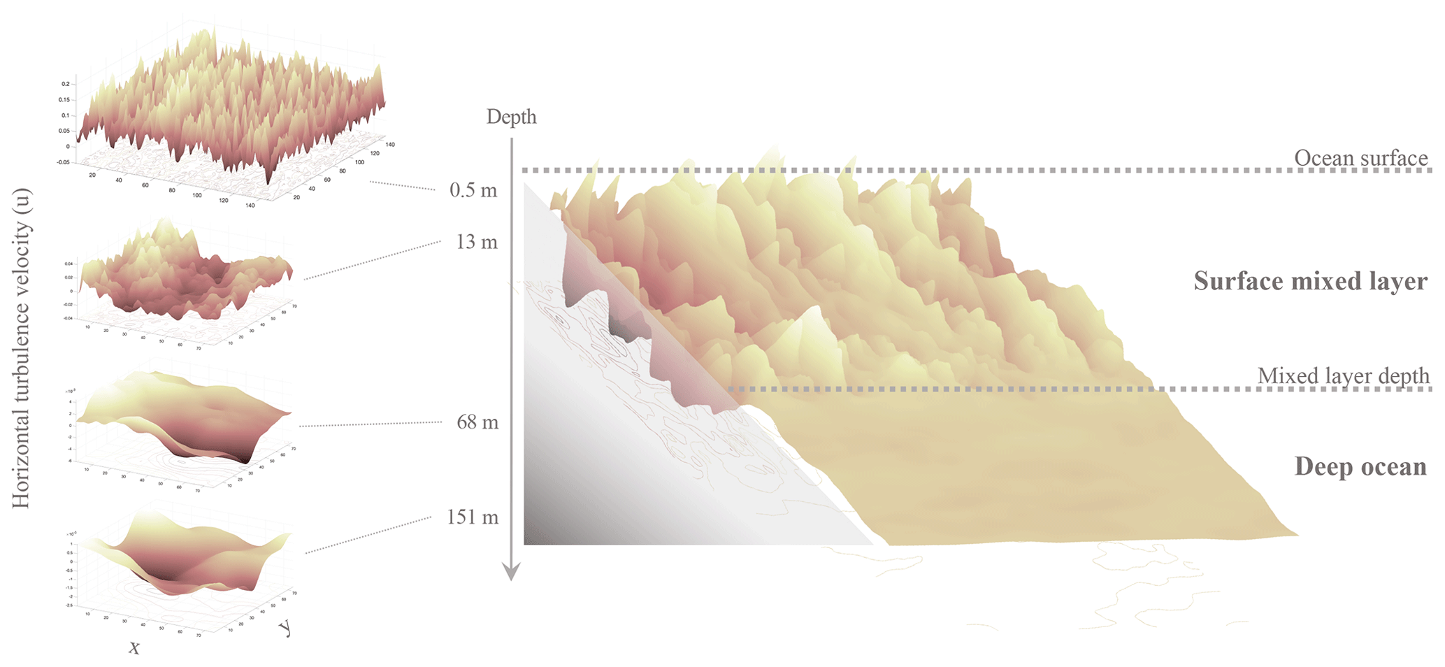
Figure 1A snapshot of a horizontal component of the water velocity simulated by CROCO changes increasing depth, illustrating the turbulent behavior of the CROCO model simulation.
The addition of a non-hydrostatic solver is a rare feature to incorporate into a coastal model such as CROCO, but some applications on small-scale coastal dynamics will require nonhydrostatic capability. The scalings of the fluid equations for common oceanographic problems (e.g., McWilliams, 1985) indicate that the dimensionless vertical momentum equation has two key parameters determining if hydrostasy will be adequate: the aspect ratio and Froude number (ratio of vertical shear to buoyancy frequency).
When non-hydrostatic effects are important, the aspect ratio approaches 1, and the stratification is not stronger than the shear, so the resulting turbulent motions are nearly isotropic.
Ocean large-eddy simulations (LESs) are usually used in the non-hydrostatic regime, and thus these models solve the non-hydrostatic equations.
Typically, non-hydrostatic ocean models also employ the Boussinesq approximation (Marshall et al., 1997). In CROCO, the implementation of non-hydrostatic physics takes advantage of compressible fluid dynamics to arrive at a simplified numerical implementation. In CROCO, the degree of compressibility can be varied by changing the speed of sound in the model, but it cannot be chosen to be infinite (i.e., incompressible). Importantly, for this paper, the speed of sound does not need to be realistic in order to simulate conditions similar to those in non-hydrostatic Boussinesq approximation LES. The lower the speed of sound is, the larger the time steps can be in CROCO, and thus the more efficient the model becomes. Section 2 explores the sensitivity of CROCO results to changing the speed of sound and other parameters that arise only in compressible fluid models.
In order to test the accuracy and computational efficiency of CROCO, an idealized ocean setting is applied as a benchmark (Fan et al., 2023c), where the proven National Center for Atmospheric Research large-eddy simulation (NCAR-LES, Fan et al., 2023b) model can be used to evaluate the performance of CROCO. The setting is doubly periodic, horizontally homogeneous turbulence forced with winds and/or convective cooling at the surface, following the class of simulations developed for the study of entrainment (Li and Fox-Kemper, 2017) and anisotropy (Li and Fox-Kemper, 2020) modeling. NCAR-LES (Moeng, 1984; Sullivan et al., 1994), PALM (Raasch and Schröter, 2001), and Oceananigans (Ramadhan et al., 2020) are branches of the LES model family which are also compared in preliminary testing to see how much those models differ. These LES models are more similar to one another than NCAR-LES and CROCO (they are all Boussinesq non-hydrostatic models, while CROCO in non-hydrostatic mode solves the compressible fluid equations), but they still differ in capabilities, numerics, code language, and subgrid schemes. The purpose of comparing these three LES models is to demonstrate the level of agreement among “standard” LES models, including the NCAR-LES model, which can serve as a guide in the NCAR-LES versus CROCO comparisons. The inter-model spread of the three LES models provides a measure of the level of uncertainty due to subgrid-scale (SGS) parameterizations, numerical schemes, etc., without the Boussinesq versus compressible fluid aspect of the NCAR-LES versus CROCO comparisons. In the subsequent analyses with CROCO, the NCAR-LES model is the focus of comparison.
In this paper, the comparisons between CROCO and NCAR-LES are divided into two major aspects: model prediction accuracy (Sect. 2) and computational efficiency (Sect. 3). The descriptions of these three LES models are presented in Sect. 2.5. In the accuracy and LES comparisons, essential turbulence statistics form the basis, and the results include the effects in CROCO of varying the explicit SGS parameterization, the second viscosity, the speed of sound, and the time step. In the efficiency comparison, the computational time for each time step is recorded to measure the model efficiency, and the factors which limit the time step in each model are discussed. Strong and weak scaling are examined in simulations set for different problem sizes and workload per processor, respectively. The impacts of varying the Message Passing Interface (MPI) parallelization of CROCO and 2D decomposition of NCAR-LES, as well as the settings of the Cheyenne supercomputer, are discussed.
In this section, we compare the turbulence statistics simulated by the NCAR boundary-layer LES model (Moeng, 1984; Sullivan et al., 1994; Sullivan and Patton, 2011) and the Coastal and Regional Ocean COmmunity (CROCO) non-Boussinesq (NBQ) model (Auclair et al., 2018; Marchesiello et al., 2021). In addition, we test the sensitivity of the turbulence statistics to certain constants specific to the CROCO NBQ model.
All simulations in this section use the following configuration. The grid has 256 uniformly spaced points in each direction (including the NCAR-LES pseudo-spectral collocation grid). The domain size is 320 m × 320 m horizontally and 163.84 m vertically. The horizontal resolution Δx=Δy is 1.25 m, and the vertical resolution Δz is 0.64 m. The vertical Coriolis parameter f is , and the horizontal Coriolis parameter is set to zero. The density ρ is given by a linear equation of state without salinity, namely , with the reference density ρ0=1000 kg m−3, reference temperature θ0=13.554 °C, thermal expansion coefficient °C−1, and potential temperature θ. Initially, there is a mixed layer with θ=14 °C above m, and below that depth, the temperature linearly decreases to 12.8 °C at z=163.84 m, providing a nearly uniform buoyancy frequency of N=0.0044 s−1 ≈43f below the mixed layer. The bottom boundary uses a rigid free-slip surface and no-flux conditions. In the fields of atmospheric dynamics and oceanography, the Brunt–Väisälä frequency, also known as the buoyancy frequency, quantifies the stability of a fluid in response to vertical displacements, such as those induced by convection. At the upper boundary, uniform wind stress in the x direction and uniform surface heat flux Q* are applied where the upper-boundary temperature flux is given by with specific heat capacity cp=3985 . The gravitational acceleration g is 9.81 m s−2. During the initial spin-up period, the wind stress and the surface heat flux increase to their full values over 51 min (5 % of the inertial period). After this period, they stay constant. Four combinations of the waterside friction velocity U* and the surface heat flux Q* are considered, namely (0.006 m s−1; 5 W m−2), (0.006 m s−1; 50 W m−2), (0.012 m s−1; 5 W m−2), and (0.012 m s−1; 50 W m−2).
The NCAR-LES model uses a two-part SGS eddy viscosity model of Sullivan et al. (1994) designed to improve the LES accuracy in comparison to the similarity theory (Monin and Obukhov, 1954) near the surface at z=0 m. Their SGS model constants Ck and Cϵ in their Eqs. (4) and (11) are 0.1 and 0.93, respectively. We configure their SGS model such that it reduces to a simpler form (their Eq. 1) below m. With rough approximations, this simpler model can be related to the Smagorinsky (1963) model with a relatively large value of the corresponding Smagorinsky constant Cs=0.18 (their Eq. 14). The NCAR-LES uses the pseudo-spectral method (Fox and Orszag, 1973) for the horizontal derivatives and second-order-centered finite differences for the vertical derivatives (Moeng, 1984). The resolved vertical temperature flux is determined using a second-order near-monotonic scheme (Beets and Koren, 1996). The higher third of wavenumbers are zeroed out to remove aliasing of unresolved scales (Orszag, 1971). The time stepping utilizes a third-order Runge–Kutta scheme (Sullivan et al., 1996). More information is given in the model description papers (Moeng, 1984; Sullivan et al., 1994; Sullivan and Patton, 2011).
The CROCO NBQ model offers several options for the SGS parameterizations. In this paper, we consider two options, namely the use of only numerical diffusion and the SGS model of Lilly (1962). The former avoids adding any explicit SGS terms and implicitly relies only on numerical diffusion. Here, the WENO5-Z improved version of the fifth-order-weighted essentially non-oscillatory scheme (Borges et al., 2008) is used for all advection terms (see Auclair et al., 2018, and Marchesiello et al., 2021, for more information). Unless explicitly mentioned otherwise, the CROCO runs shown here use the numerical-only option for the SGS parameterization because we are interested in understanding the performance of (unavoidable) numerical diffusion before adding explicit SGS terms (and associated parameters) which make the model behavior more complex. We test the explicit SGS effect only briefly in Sect. 2.2.
2.1 NCAR-LES model vs. CROCO NBQ model
Here, we compare the NCAR-LES model with the CROCO NBQ model. As we will see shortly, the results show that these two models produce very similar boundary-layer flows, with differences comparable to those among the different LES (Sect. 2.5).
The CROCO model uses a time-splitting method and uses two different time steps for the so-called fast and slow modes. In this subsection, all of the CROCO runs use a slow-mode time step of 0.5 s and a fast-mode time step of 0.019 s. We tested many different time steps, and these values are closest to the largest stable values for the configuration used. To match the slow-mode time step, the NCAR model runs in this section use a time step of 0.5 s as well. However, note that the NCAR model can be run with a much larger time step, and it has the capability of adjusting its time step based on an embedded Runge–Kutta multiple-order approach; namely, the Courant–Friedrichs–Lewy (CFL) time step which the NCAR model finds when running with adjustable time-stepping is about 7 s for the runs with m s−1 and about 3 s for the runs with m s−1. Thus, when used with this reduced time step, the NCAR model is roughly 6 to 14 times slower.
The CROCO NBQ model has two constants related to the fast mode, namely the speed of sound cs and the second viscosity (also called bulk viscosity, volume viscosity, or dilatational viscosity) λ. Because we are not interested in sound waves, we may use an unphysically small value of cs and an unphysically large value of λ to relax the sound-related CFL constraint by slowing and damping these waves, respectively. In this subsection, we use cs=3 m s−1, and , which are about 500 times slower and 400 times more viscous than in seawater. As discussed in Sect. 2.4 and 2.3, the unphysical values of these constants affect turbulence statistics negligibly.
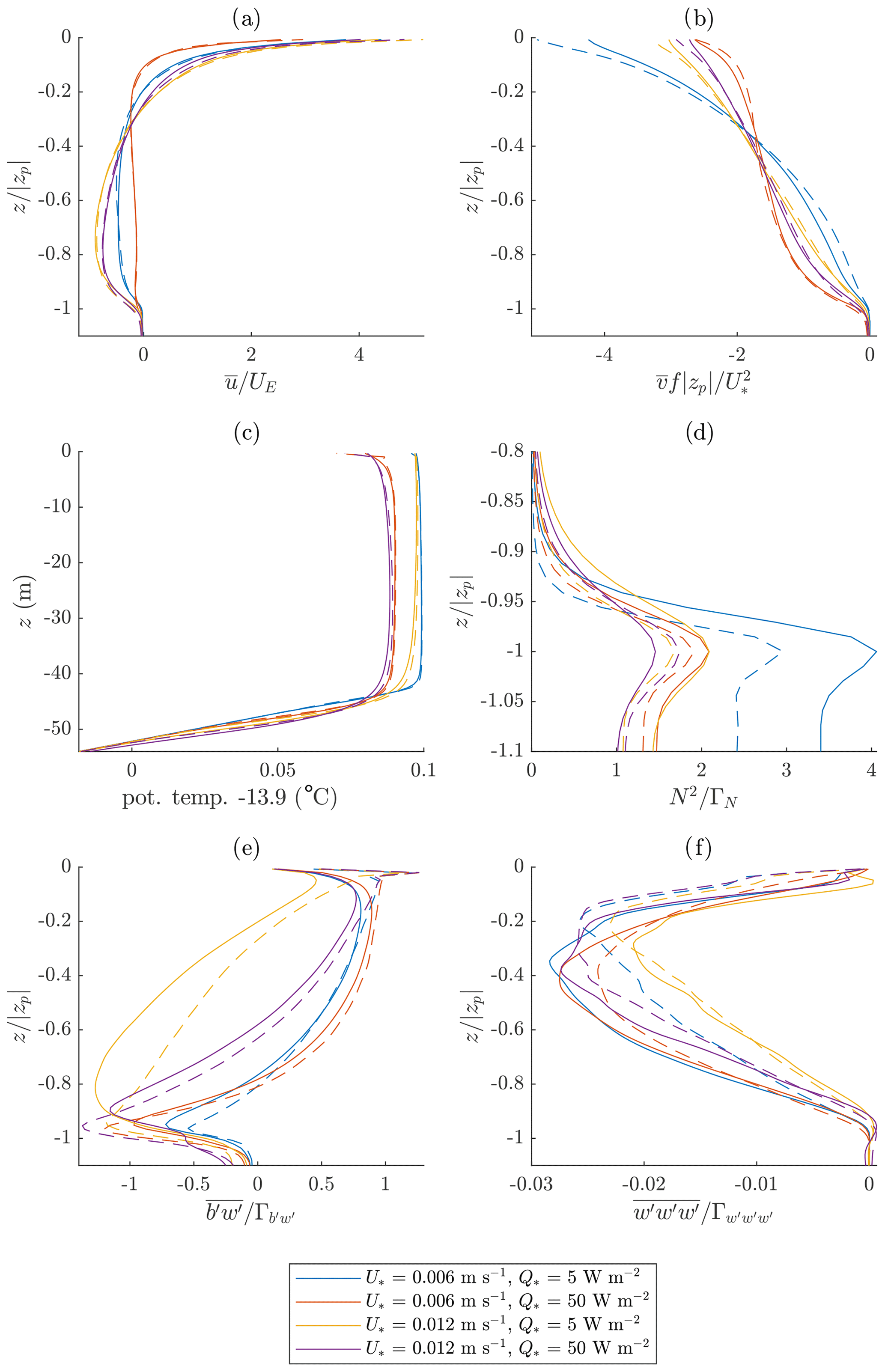
Figure 2Comparison between the NCAR-LES model (solid) and the CROCO NBQ model (dashed). The line color indicates the surface forcing as shown in the legend.
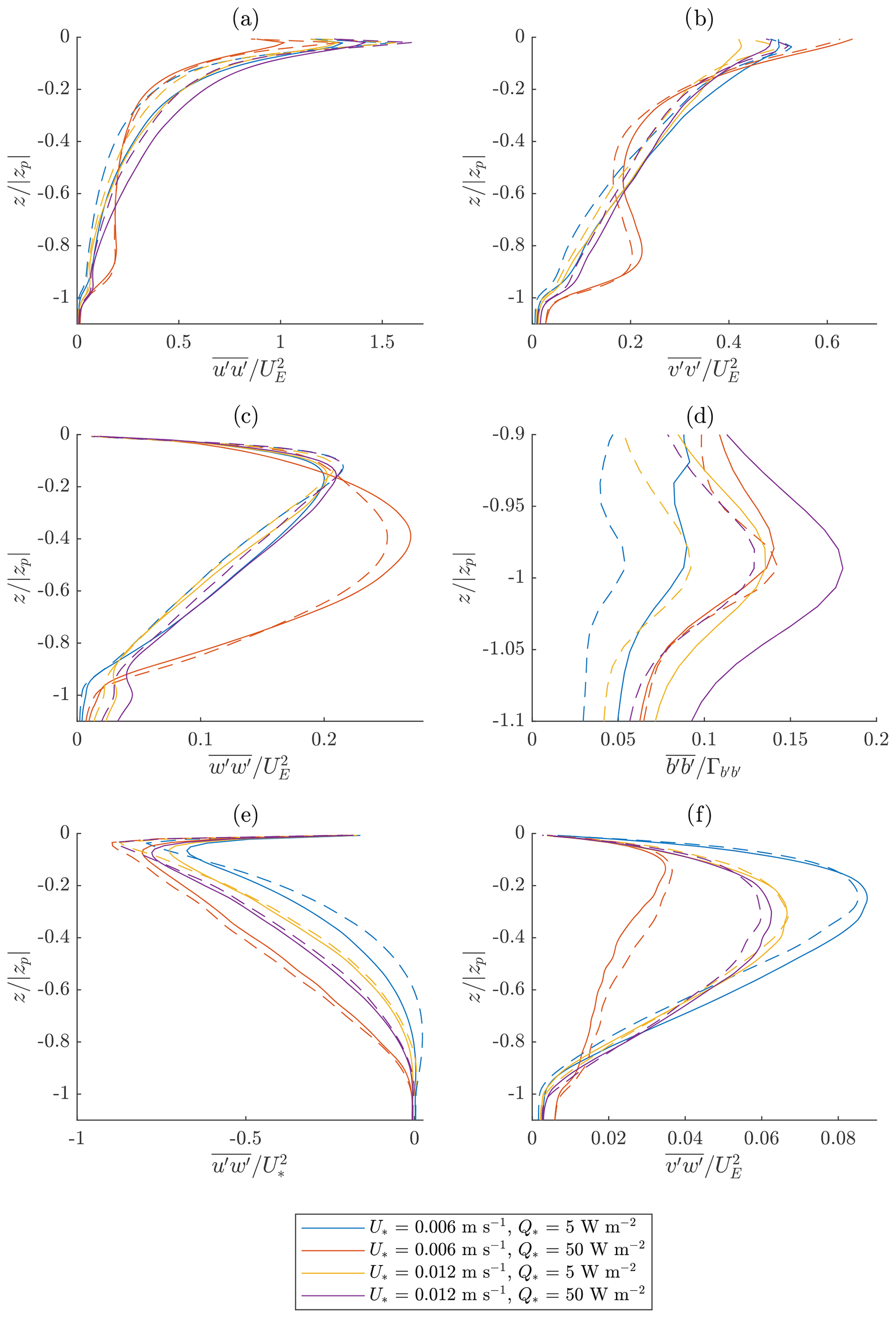
Figure 3Comparison between the NCAR-LES model (solid) and the CROCO NBQ model (dashed). The line color indicates the surface forcing as shown in the legend.
Figures 2 and 3 show the vertical profiles of various flow properties.1 Hereafter, we use the following symbols: the horizontal average and the turbulent fluctuation for any quantity ϕ, the buoyancy , the buoyancy frequency , and the horizontally averaged depth zp of the mixed-layer base defined as the z coordinate of the N2 maximum.
2.1.1 Scaling of turbulent properties
To understand these figures, let us first explain the non-dimensionalization used. Figures 2a and 3a, b, c, and f show quantities related to the turbulent kinetic energy (TKE) and the TKE shear production, such as the mean shear and a Reynolds stress component. These quantities are largely governed by the energy input to the water rather than the wind stress or surface heat flux. Therefore, we introduce a characteristic scale E* of the surface energy flux:
where is the surface current in the wind stress direction, and is the surface buoyancy flux. The first term on the right-hand side is the flux of the work done by the wind stress, and the second term is a rough approximation of the flux of available potential energy.2 For ease of notation, we use an energy-flux-based velocity scale
While and are also related to the TKE shear production, they are largely constrained by other factors. Therefore, we use other scalings to non-dimensionalize them. Figure 2b uses the vertically averaged Ekman transport velocity because is roughly constrained by the Ekman balance. Figure 3e uses the wind stress because is constrained by the wind stress.
In Fig. 2d, we use a stratification-scale ΓN pertinent to pycnocline entrainment, where
and Δe is a length scale3, and
is a rough depth scale of the wind-driven boundary layer4, and
is a rough scale of the energy flux at zp causing pycnocline entrainment.5 Unlike the available potential energy input, the wind energy input is largely dissipated near the surface and is not directly used for pycnocline entrainment. Therefore, Eq. (7) assumes an exponential decay of the wind energy available to pycnocline entrainment. Note that, for a pycnocline buoyancy frequency , is the energy necessary to mix the Δe thickness of the pycnocline water with the adjacent mixed-layer water located between zw and zp where mostly the convective turbulence has to entrain the pycnocline water and lift it up to the Ekman-layer bottom zw (where a larger amount of wind energy is available for the mixing above). Therefore, the normalized-buoyancy frequency in Fig. 2d indicates how strong the pycnocline stratification is relative to the energy input available for the pycnocline entrainment.
In Fig. 2e, we use a two-part buoyancy flux scale
where the first term is the scale relevant near the surface, and the second term is the scale relevant near the boundary-layer bottom. The non-dimensional constant in the second term is used only to make the normalized value at zp close to −1.
Figure 2f uses the energy-flux-based scale for but modified with a non-dimensional function ϕs as
because is very sensitive to the turbulence structure. When , the turbulence develops distinct convective rolls spanning the whole boundary-layer depth, while in other cases convective rolls are much weaker, and the turbulence structures in the upper part of the boundary layer are more similar to the pure wind-driven turbulence – which mainly consists of smaller-scale and more disturbed tilted vortexes – and the turbulence structures in the lower part of the boundary layer are similar to pure convective plumes. Convective rolls utilize both wind energy and available potential energy constructively and channel these energies into bands of strong w′. In contrast, the turbulence in the other cases uses wind energy to mix the water in the upper part of the boundary layer and thereby partially distracts the available potential energy coming in from the surface. As a result, due to convective rolls is much stronger. Therefore, to make the order of the normalized values similar, we use ϕs=5 when and ϕs=1 otherwise.
Figure 3d shows near zp. It is dominated by internal waves and isopycnal deformation due to the boundary-layer turbulence reaching zp. The non-dimensionalization is done relative to the stratification and the energy input to these processes, namely
2.1.2 Comparison of results
Figure 2a, b, and c show that the simulated mean flows are very similar. The only somewhat notable differences are (1) that the CROCO surface velocity tends to be slightly higher, (2) that the CROCO surface temperature tends to be slightly lower, and (3) that the CROCO pycnocline entrainment is weaker. The weaker entrainment in CROCO can be seen more clearly in the comparison of the deepening mixed layers in Fig. 4.
The CROCO runs produced weaker mixed-layer deepening, although Fig. 2d shows that CROCO runs had either a similar or greater amount of energy flux reaching the mixed-layer base.6 Furthermore, despite the slower mixed-layer deepening in the CROCO runs, CROCO tends to have a slightly stronger resolved buoyancy flux at the mixed-layer base (Fig. 2e). This implies that the NCAR model's faster entrainment occurs because NCAR model's explicit SGS diffusion is larger than CROCO's implicit (numerical-only) SGS diffusion. Note that the NCAR model also has only second-order advection in the vertical with up-winding, so even though it is centered, it may have higher-order diffusion and dispersion effects, while CROCO has fifth-order advection with implicit diffusion entering only at the highest orders. This point is reiterated in Sect. 2.2, where we add explicit SGS diffusion terms to a CROCO run.
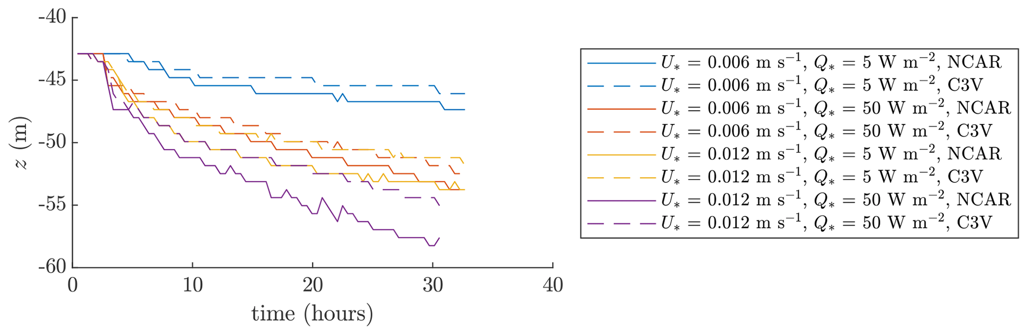
Figure 4Time series of the mixed-layer base depth zp. C3V in the legend refers to the CROCO NBQ run with the speed of sound cs=3 m s−1 and the second viscosity . The difference in the mixed-layer deepening occurs mainly because NCAR's explicit SGS diffusion is larger than CROCO's implicit SGS (that is, only numerical) diffusion.
Figures 2e and f and 3a, b, c, e, and f show that the resolved turbulence statistics are overall very similar. Note that a difference of up to about 10 % should be considered negligible for the domain size used and the time window lengths used for averaging. Experimentation by varying time steps (not shown) gives this level of difference, reflecting that different realizations of instantaneous chaotic turbulent flow that do not alter the turbulence statistics can differ by this amount. This order of difference is likewise justified by the comparison among the LES in Sect. 2.5, which approach 10 % differences in many of the same variables even though the averaging in those LES comparison figures is over an entire inertial period. Especially, the profiles of , , and fluctuate strongly and require significant averaging to obtain a well-sampled profile. However, near the surface, where the turbulence structures tend to be small, the statistics are more robust even for these quantities. Thus, the resolved turbulence quantities near the surface tend to be robustly stronger for the CROCO runs. This stronger resolved turbulence is closely related to the difference in the SGS parameterization, which becomes significant near the surface. Generally, a stronger SGS diffusion tends to weaken the resolved turbulence. Therefore, the result here suggests that CROCO's numerical diffusion is weaker than the explicit SGS diffusion of the NCAR model. As shown in Sect. 2.2, the difference in the resolved turbulence quantities significantly reduces when the CROCO model uses an explicit SGS diffusion additionally to the (unavoidable) numerical diffusion.
Figures 3c and d show that the variances of the resolved w and b in the stratified part of the water () tend to be larger with the NCAR model. This is partially due to the slightly smaller UE and Eb in the NCAR runs. However, this tendency persists in the dimensional variances as well. Contrary to these variances, the resolved buoyancy flux (Fig. 2e) at the same depths tends to be less with the NCAR model. Therefore, the NCAR runs have stronger internal waves (that have no buoyancy flux when they are not growing or decaying) and less resolved turbulent mixing. It is not clear why this is the case, but one hypothesis was that these waves are more easily supported by the horizontal pseudo-spectral numerics of the NCAR-LES, and another hypothesis is that the fifth-order WENO (weighted essentially non-oscillatory) scheme in CROCO is damping these waves. Further experimentation with different numerics in CROCO is possible but is beyond the scope of this comparison paper. However, no similar effect is seen when comparing the different LES schemes in Figs. 10–11.
To further investigate this difference, the spectra of 1D discrete fast Fourier transform (FFT) modes and the circularly integrated 2D energy spectra of u′, v′, w′, and b′ are shown in Figs. 5 and 6. These figures are made using the data taken from special runs with a larger horizontal domain size of 640 m × 640 m in order to have more wavenumbers and for better statistics, and the results are very similar to the baseline domain size of 320 m × 320 m. These spectra are taken from three different regions, namely the mixed-layer interior ( m), the entrainment layer ( m), and the pycnocline interior ( m). Overall, the NCAR and CROCO simulations tend to differ with respect to the spectral heads and tails. The difference in the high wavenumber tail is likely due to the dealiasing truncation in the NCAR runs which is not likely to resemble the high wavenumber numerical diffusion in the CROCO approach. Note that this difference occurs over roughly the upper third of wavenumbers for which the dealiasing is applied. The deviations at low wavenumber are due to the integral constraints of 〈w〉=0 and due to the buoyancy anomaly over the whole domain being linked to vertical fluxes. Thus, the small-scale deviations and large-scale deviations are linked. In u’ and v’, there are not meaningful large-scale deviations. We show only the spectra from the case with because the differences between the NCAR and CROCO simulations have similar tendency for all other cases.
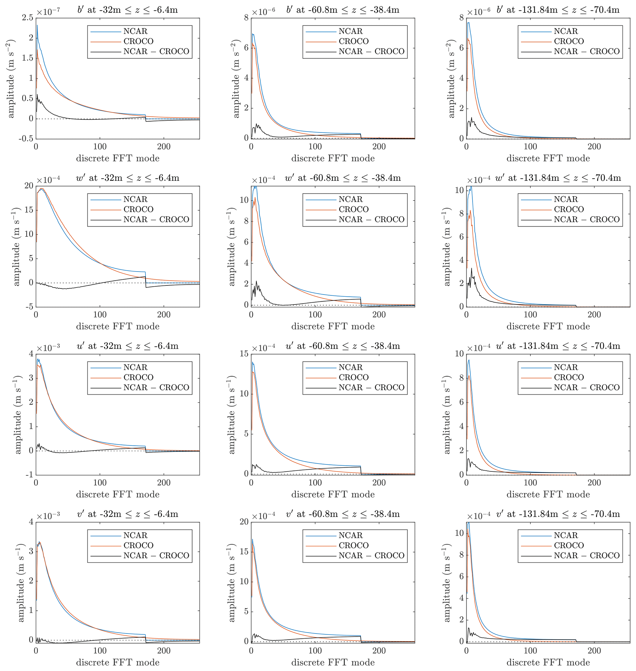
Figure 5Comparison of the 1D discrete FFT spectra with . Each spectrum is smoothed by averaging over the vertical range shown in each title, as well as averaging over 21 h and each horizontal direction.
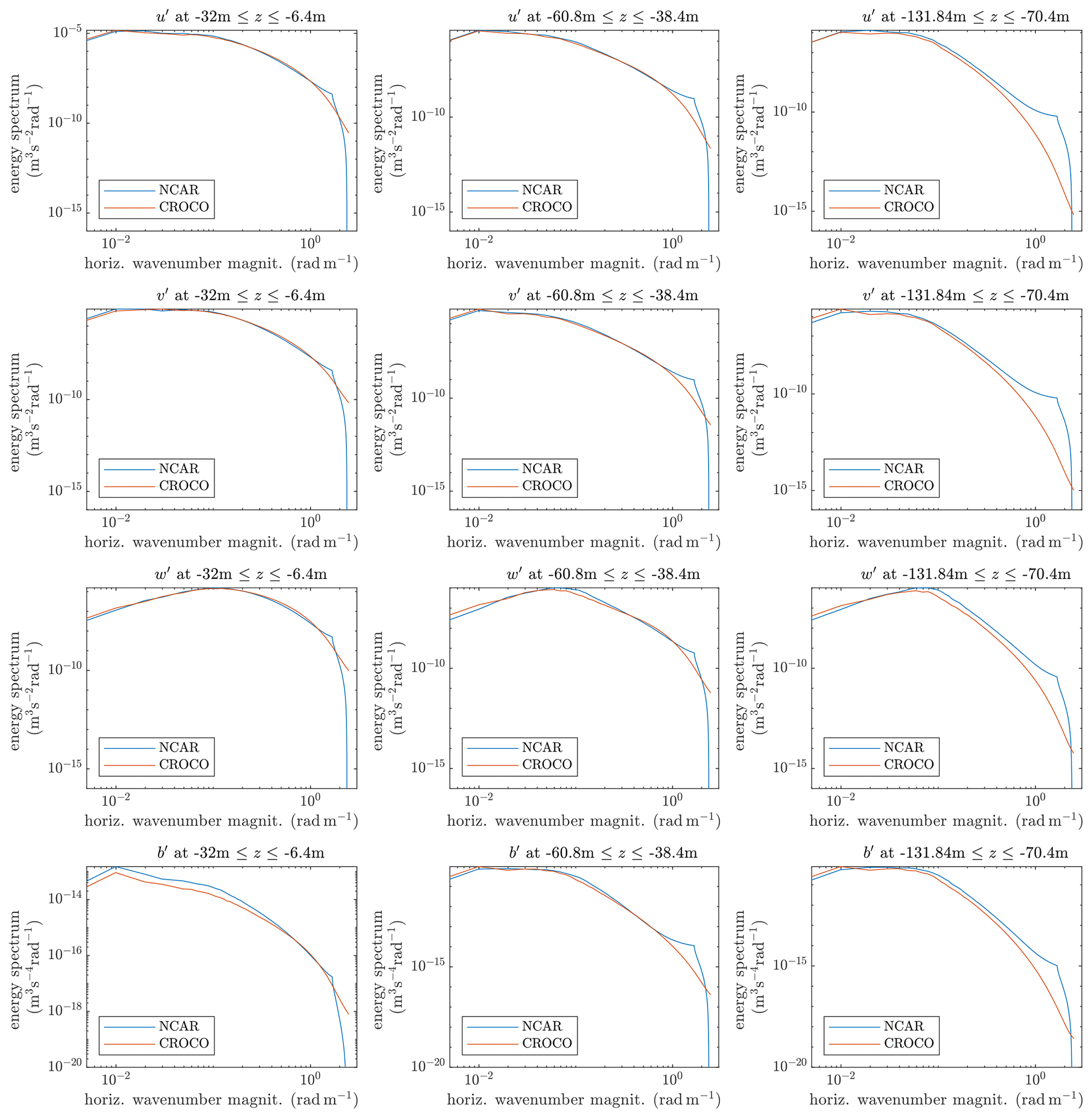
Figure 6Comparison of the 2D spectra averaged in circular rings at constant horizontal wavenumber magnitude from the runs with . Each spectrum is smoothed by averaging over the vertical range shown in each title, as well as averaging over 21 h.
2.2 The effect of the explicit SGS parameterization
This subsection shows how explicit SGS diffusion terms affect the results in Sect. 2.1. For this reason, we focus on the case with because this case has the largest difference in the mixed-layer deepening, which is the most significant difference observed in the previous subsection. Here, the CROCO NBQ run uses a modified version of the SGS parameterization by Lilly (1962), namely
where
and the indexes are , , and . The summation convention is used, and the model parameters are the Smagorinsky constant Cs, Prandtl number Pr, and a mixing threshold constant CR. The SGS terms become zero when a Richardson-like number exceeds CR. As mentioned in the introduction to Sect. 2, the NCAR model's SGS parameterization below m is roughly relatable to the Smagorinsky model with Cs=0.18. Therefore, we test Cs=0.17 and 0.2 with CROCO. These values of Cs, together with a large value of Pr, produce the mixed-layer deepening comparable to the NCAR model run, as shown in Fig. 7, where the mixed-layer deepening with (0.17, 0.25, 3) and (0.2, 1, 4) is shown. Note also that the net entrainment in the CROCO implicit plus explicit diffusion cases (C3VS and C3VS2) is greater that the implicit-only diffusion, which is important to verify as occasionally net effects can in fact become larger under implicit-only diffusion if the gradients sharpen in response (Bachman et al., 2017). The results in Fig. 7 demonstrate that the difference in the entrainment and mixed-layer deepening seen in the previous subsection is due primarily to the SGS parameterization always present in the NCAR-LES, and the numerical-only diffusion of the CROCO runs is less than the combined numerical plus explicit diffusion of the NCAR model and the C3VS cases.
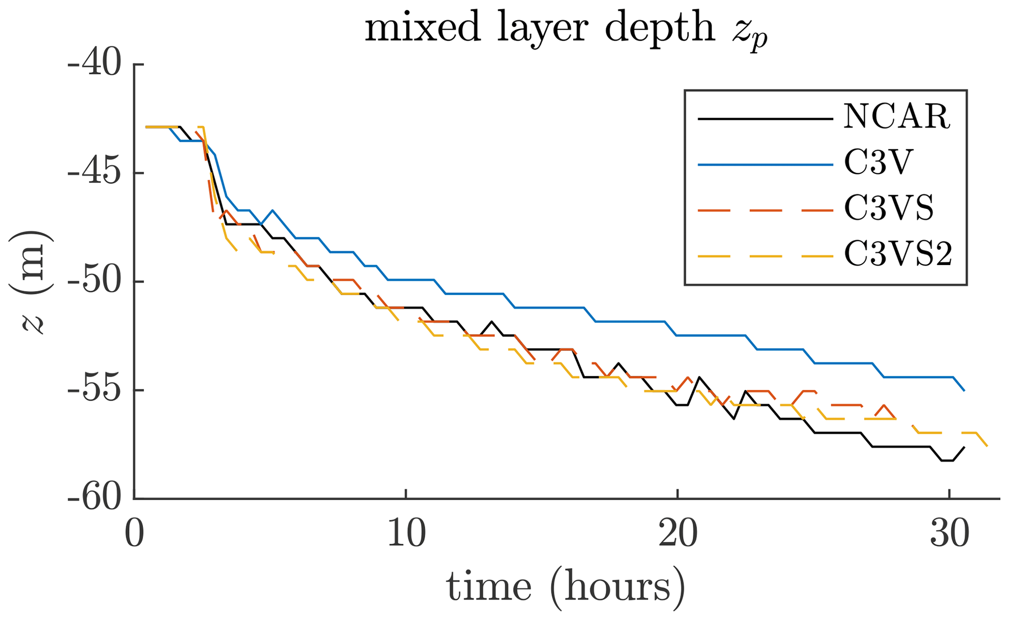
Figure 7Time series of the mixed-layer base depth zp. The CROCO NBQ runs (C3V, C3VS, and C3VS2 in the legend) use the speed of sound cs=3 m s−1 and the second viscosity . C3V uses only numerical diffusion. C3VS and C3VS2 use an explicit SGS parameterization (11)–(18) with (0.17, 0.25, 3) and (0.2, 1, 4), respectively.
The previous subsection also showed that the resolved turbulence quantities near the surface tend to be larger with the CROCO model without an explicit SGS parameterization. This difference also significantly reduces with the addition of the explicit SGS parameterization, as shown in Figs. 8 and 9.7
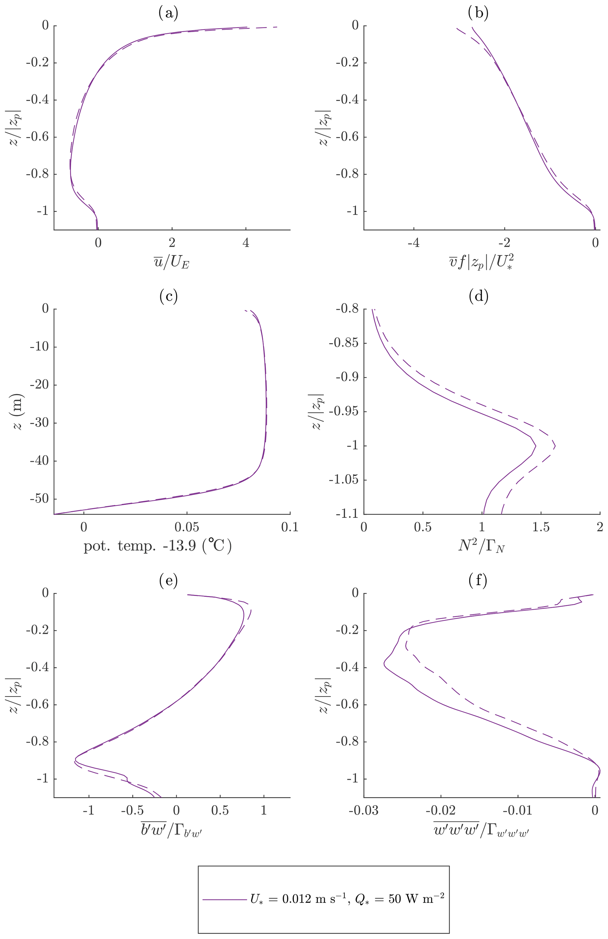
Figure 8Comparison between the NCAR run (solid) and the C3VS CROCO run (dashed) including explicit SGS dissipation with (0.17, 0.25, and 3). Compare this to the purple lines in Fig. 2 which show the same forcing but for the CROCO C3V case with only implicit dissipation.

Figure 9Comparison between the NCAR run (solid) and the C3VS CROCO run (dashed) including explicit SGS dissipation with (0.17, 0.25, 3). Compare this to the purple lines in Fig. 3 which show the same forcing but for the CROCO C3V case with only implicit dissipation.
A stronger near-surface diffusion weakens the resolved turbulence. There are some small remaining differences, but they are expected because different explicit SGS parameterizations are used in the NCAR and CROCO models.
In summary, the NCAR results and the CROCO results are overall very comparable. There are some minor differences, but most of them are due to the different SGS parameterization. The only notable difference that may not be attributable to the SGS parameterization difference is that the NCAR model runs tend to produce more internal waves in the stratified part.
2.3 The effect of the second viscosity parameter
For the CROCO NBQ model runs, an unphysically large value of the second viscosity λ may be used to aggressively dissipate (near-grid-scale) pseudo-acoustic waves and stabilize the simulation. Therefore, we tested whether an unphysically large value of λ affects the turbulence statistics. We evaluated two types of CROCO runs having the speed-of-sound parameter cs=202 m s−1. One simulation uses , and the other uses for and for all other values of . The results show that the turbulence statistics are not significantly affected.
By increasing λ, the additional viscosity does have the effect of stabilizing marginal numerical instabilities so that the optimal slow-mode time step increases from 0.15 s to 0.2 s for the case with (0.006 m s−1; 5 W m−2) and from 0.04 s to 0.08 s for the cases with (0.012 m s−1; 5 W m−2) and (0.012 m s−1; 50 W m−2). However, for the case with (0.006 m s−1; 50 W m−2), increasing λ does not lead to an increase in the slow-mode time, which stays at 0.25 s. The optimal fast-mode time step is unaffected by λ and is about 0.0038 s for all values of . Therefore, increasing damping using λ speeds up the simulations only slightly.
2.4 Sensitivity to the speed-of-sound parameter
Reducing the speed-of-sound parameter cs in the CROCO NBQ model allows a larger time step by relaxing the CFL condition related to pseudo-acoustic waves. Here, we study the effect of reducing the value of cs to a value 500 times slower than nature, cs=3 m s−1. The results show that the resolved turbulence statistics are largely insensitive to the value of cs between cs=3 m s−1 and cs=202 m s−1. However, it should be noted that cs should not be smaller than the fastest speed of the process that needs to be properly simulated (for example, the barotropic wave speed in the case of geophysical applications).
Most statistics have only small differences that should be considered negligible for the given limited domain size (not shown). The only possibly non-negligible difference appears in the internal wave strength seen below for the cases with m s−1. It is unclear why the intensity of internal waves is sensitive to changing the speed of sound. However, note that the differences among the two CROCO simulations that differ in terms of the speed of sound are not as big as the differences between the NCAR and CROCO internal wave strength in previous comparisons.
Decreasing cs without increasing λ makes simulations unstable and is not recommended. By decreasing cs together with increasing λ, the optimal slow-mode and fast-mode time steps increase to 0.5 and 0.019 s, respectively, for all optimized runs, amounting to more than 5 times faster simulations.
2.5 Comparison between LES models
NCAR-LES was developed at NCAR to simulate planetary-boundary-layer turbulence (Moeng, 1984) and extended to include the effects of ocean surface waves when applied to the ocean-surface-boundary-layer turbulence (McWilliams et al., 1997). The spatial discretization is pseudo-spectral in the horizontal and the finite difference in the vertical. It uses a modified Smagorinsky subgrid-scale (SGS) closure that evolves a prognostic equation for the SGS turbulent kinetic energy (TKE) (Deardorff, 1980; Sullivan et al., 1994).
The Parallelized Large-Eddy Simulation Model (PALM) was developed at Leibniz Universität Hannover (Germany) as a turbulence-resolving LES model for atmospheric- and oceanic-boundary-layer flows, specifically designed to run on massive parallel computer architectures (Raasch and Schröter, 2001; Maronga et al., 2015). It uses a modified version of the Deardorff (1980) SGS parameterization similar to the NCAR-LES. But the spatial discretization is finite differences in both the horizontal and vertical directions. An upwind-biased fifth-order differencing scheme for advection terms in combination with a third-order Runge–Kutta time-stepping scheme is used in PALM (Wicker and Skamarock, 2002).
Both NCAR-LES and PALM have been widely used in simulating atmospheric- and oceanic-boundary-layer turbulence under various idealized and realistic conditions, while Oceananigans is a new (v0.83.0 is used here), fast, and user-friendly software package for numerical simulations of geophysical fluid dynamics developed at the Massachusetts Institute of Technology in the Julia programming language (Ramadhan et al., 2020). Oceananigans uses a spatial discretization that is a finite volume, and it can be configured as an LES with various combinations of SGS, advection, and time-stepping schemes. For this particular comparison, we are using the anisotropic minimum dissipation closure (Verstappen, 2018) combined with third-order Runge–Kutta time-stepping and fifth-order WENO advection.
Ideally, the differences in the discretization and SGS closure schemes among the three LES models should not affect the horizontally and temporally averaged turbulence statistics for the ocean-surface-boundary-layer problem, as long as the grid cells are small enough to capture the dominant turbulent structures and the model domain is large enough to collect robust statistics. Here we assess to what extent this assumption is valid using two idealized cases: a case dominated by wind-driven shear turbulence with and a case dominated by convective turbulence with . In both cases, we run PALM and Oceananigans using a consistent domain size and resolution such as NCAR-LES.
Figures 10 and 11 compare the vertical profiles of the horizontal mean turbulence statistics averaged over the last inertial period (∼ 17 h) for the two idealized cases, respectively. As expected, the three LES models give largely consistent results for the turbulence statistics examined here in the two idealized cases. The most notable differences are confined near the surface or at the base of the boundary layer where entrainment is important, which highlights where the differences in SGS closure and numerical schemes have their greatest impact (note that the turbulence statistics shown here are all well resolved). The seemingly large discrepancies in Figs. 10c and 11a, d are due to the normalization and constraints imposed at the surface; the buoyancy flux is small in the wind-driven shear-turbulence-dominant case, and the momentum flux is small in the convective-turbulence-dominant case. Thus, the variables which are most strongly forced at the surface are in closest agreement when normalized by the surface forcing (Li and Fox-Kemper, 2017; Skitka et al., 2020). Indeed, the simulated momentum flux in the first case (Fig. 10d) and buoyancy flux in the second case (Fig. 11) show the best agreement among the three LES models. The vertical velocity skewness (), cross-wind velocity component (), temperature variance (), and stratification () (Fig. 10b, e, and f and Fig. 11b, e, and f) are not as strongly constrained by the surface forcing and are subject to more variability among the models, especially at the surface and base of the boundary layer where entrainment occurs.
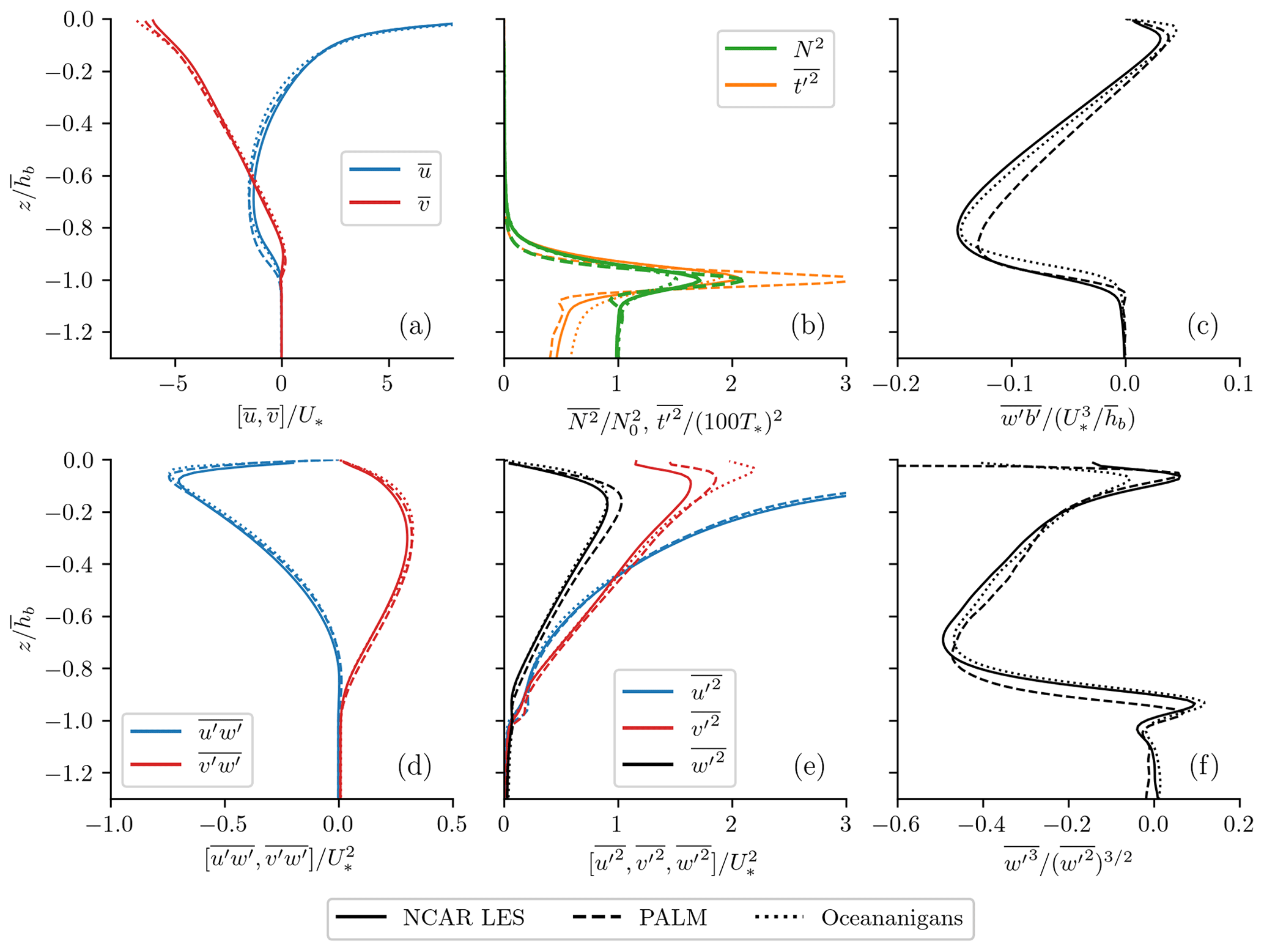
Figure 10A comparison of the horizontally and temporally averaged turbulence statistics among NCAR-LES (solid), PALM (dashed), and Oceananigans (dotted) in a case dominated by wind-driven shear turbulence. The normalized turbulence statistics include (a) horizontal velocity, , normalized by the friction velocity U*; (b) stratification (black), , normalized by its value below the boundary layer, , and temperature variance (purple), , and normalized by a characteristic temperature ; (c) buoyancy flux, , normalized by , hb refers to the mixed-layer depth; (d) momentum flux, , normalized by ; (e) velocity variance, , normalized by ; and (f) the skewness, . The turbulence statistics are averaged over the last inertial period (∼ 17 h) to reduce the effects of inertial oscillation.
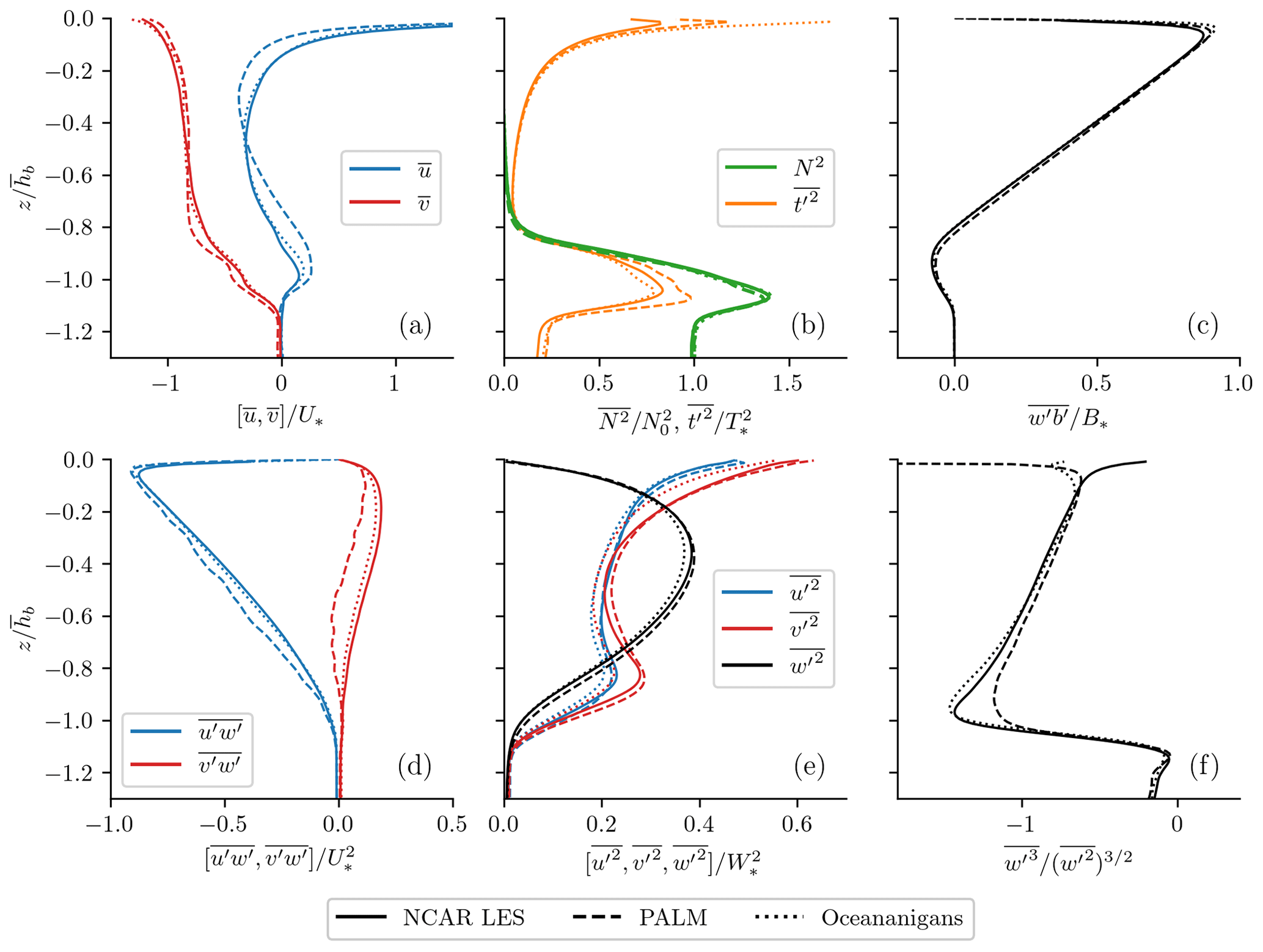
Figure 11Same as Fig. 10, except that the turbulence statistics are for a case dominated by convective turbulence, and the buoyancy flux in panel (c) is normalized by the surface buoyancy flux B*. The three components of the velocity variance in panel (e) are normalized by , where is a convective velocity scale.
2.6 A rough comparison between vertically stretched CROCO and NCAR-LES
In reproducing Li and Fox-Kemper (2017) with both NCAR-LES and CROCO, there were notable differences. However, in that comparison, many parameters differed between the models (e.g., stretched vertical grid and subgrid model) in addition to the numerics. Hence, a more detailed comparison in which gridding was more tightly matched and subgrid schemes were explored was carried out (see the preceding subsections in Sect. 2). In this final subsection, a comparison between CROCO and NCAR-LES in more typical configurations (where they are not matched in gridding and subgrid schemes) is shown to illustrate discrepancies under more realistic configurations. The preceding comparisons were motivated by the desire to better understand a set of calculations comparing CROCO to NCAR-LES under realistic conditions and typical setups for CROCO and NCAR-LES in 16 previously published scenarios with different combinations of surface wind and cooling from Li and Fox-Kemper (2017). Surface wind and cooling conditions are correspondingly matched for each case. Similar to the accuracy comparisons above, the simulation cases of both CROCO and NCAR-LES models are based on the domain size of 320 m × 320 m × 163.84 m in the directions. The computational cells are grids in each direction, which corresponds to a horizontal resolution of m. The vertical grids of the NCAR-LES are uniform, with a vertical resolution of dz=0.64 m. The vertical grids of CROCO, however, were unequal. The CROCO grid points were stretched to be finer near the surface and coarser near the bottom of the domain, as is commonly configured in CROCO and other ROMS applications.
These comparisons spanned a wider range of convective forcing (over a factor of 100) and a wider range of wind stresses (a factor of 4) than the comparisons in the previous sections. The largest differences among the simulations, however, were consistent with the preceding results. According to the comparison of horizontal () and vertical () momentum flux and the turbulence kinetic energy (TKE), the turbulence intensity was slightly weaker in CROCO, which is a similar result to the tendencies in the above comparisons. However, as we have seen in some cases, this difference can change according to the SGS scheme and averaging windows. Following a comparison of the buoyancy frequency (N2) and vertical buoyancy flux (), CROCO had weaker vertical heat transport and entrainment, similar to the differences observed in Figs. 2 and 3, and now these differences can be largely attributed to differences in SGS dissipation rather than numerics. Overall, these comparisons suggest that even in the case of a moderately stretched vertical grid, comparable results are to be expected from CROCO as in a uniform grid LES.
Many factors affect the model computing efficiency, such as the structure and assignment of computing platform, MPI parallelization, 2D decomposition of the model, and some specific physical parameterizations, particularly ones that have consequences for the stability and allowable time step size. In this section, we compared the computational efficiency of the CROCO and NCAR-LES models.
3.1 Computing platform – Cheyenne supercomputer
The number and allocation of nodes and processors used for computing and the availability of threads matter for the model efficiency. In this study, the Cheyenne supercomputer is used for efficiency tests. The Cheyenne supercomputer, built for NCAR, operates as one of the world’s most energy-efficient and high-performance computers. Cheyenne consists of 4032 dual-socket nodes with 2.3 GHz Intel Xeon E5-2697V4 processors with 18 cores each for a total of 145 152 cores and a peak performance of 5.34 PetaFLOPS. Nodes have either 64 GB or 128 GB RAM (DDR4-2400) and networked using Mellanox EDR InfiniBand high-speed interconnects with a bandwidth of 25 GBps, bidirectional, per link. The simulations presented in this paper all ran on Cheyenne with exclusive use of the nodes. In each efficiency test, the number of nodes, the number of CPUs per node, the number of MPI processes, and the number of OpenMP threads can be specified.
Combinations of nodes and CPUs per node with different problem sizes and the total number of processors were tested. When the problem size and total number of processors are fixed, we find that the combination of more nodes and fewer CPUs per node makes the CROCO model compute more efficiently. When fewer processors per node are used, most systems still typically charge for the unused processors on each node, so this is not more efficient overall; it is just more efficient per processor in use. However, this combination of the selection of nodes and CPUs per node is more costly, and so it is typically better to stick to affordable and moderate numbers despite the higher performance because more nodes requested to Cheyenne make jobs wait longer in the waiting queue and thus the overall time to complete runs is longer although the computing time is shorter.
3.2 NCAR-LES 2D decomposition
NCAR-LES uses pseudo-spectral discretization in the horizontal. Fast Fourier transforms (FFTs) are used to evaluate horizontal derivatives, which requires global data at all grid points in the direction along which the derivatives are evaluated. Thus, a simple domain decomposition in the two horizontal directions would need the frequent exchange of a large amount of data between different processors, which limits the computational performance. To address this, a 2D domain decomposition is used in NCAR-LES (Sullivan and Patton, 2008) in which each processor operates on constricted “pencils” that include all the grid points in a specific direction so that horizontal derivatives along that direction can be evaluated on a single processor with FFT. To evaluate the derivatives in the other direction, a transpose is performed before the evaluation of derivatives, and another transpose is performed afterwards. The combination of transposes and ghost point exchange uses specific communication patterns between only the subsets of processors, and no global communication is needed. Therefore, large numbers of grid points can be used, and it scales pretty well on thousands of processors. The 2D decomposition of NCAR-LES is schematized in Fig. 12, which illustrates the structure of the total number of processors used in the computational process.
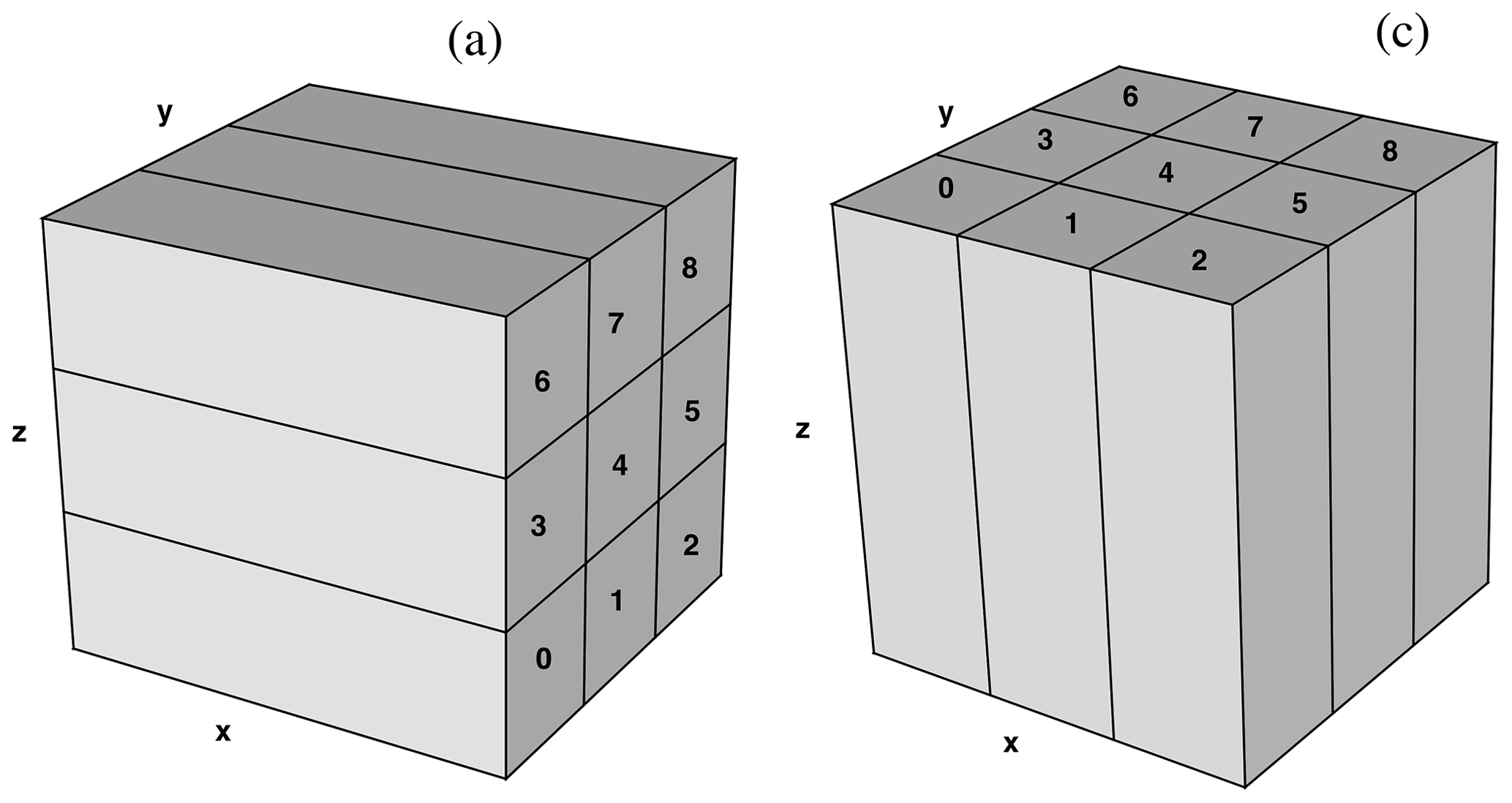
Figure 122D domain decomposition on nine processors. (a) Base state with y–z decomposition. (b) x–y decomposition used in the tridiagonal matrix inversion of the pressure Poisson equation (Sullivan and Patton, 2008).
3.3 CROCO MPI parallelization
CROCO is currently supported by two parallelization options, MPI and OpenMP, which, respectively, represent distributed memory and shared memory. The awareness of CROCO MPI or OpenMP settings is necessary to be defined as needed, and the use of MPI or OpenMP is exclusive. According to the test results, when the OpenMP is not called for during compilation in CROCO, the computing time with or without OpenMP threads on Cheyenne does not affect timing, so it offers no advantages. In this paper, CROCO is used without OpenMP and with MPI, which means only one thread is used for each processor on Cheyenne, and the decomposition of processors and distribution across nodes impact the computing efficiency. The following discussion focuses on the MPI parallelization option.
The structure of CROCO MPI decomposition is divided into the XI and ETA direction, NP_XI and NP_ETA, in CROCO, and the codes represent the number of the processor assignment in XI and ETA horizontal directions, respectively. When NP_XI =3 and NP_ETA =3 are set, the MPI parallelization structure is shown in Fig. 12c. In order to match the number of processors used in Cheyenne, the product of NP_XI and NP_ETA should be as the same as the product of the number of nodes, and the number of CPUs per node should also be matched. Different combinations of NP_XI and NP_ ETA were tested under the frameworks of different combinations of the problem size and total number of processors in the Cheyenne environment.
3.4 Efficiency test results
The performance of the model efficiency for varying problem sizes and workload per processor are shown in Figs. 13 and 14. NP = NPz × NPx × NPy, where NPz, NPx, and NPy are the number of processors in the vertical and horizontal directions, respectively. In each figure, the vertical axis is the computing time per time step t multiplied by NP and divided by total work size (i.e., number of grid points or a similar work with a logarithmic multiplier to handle the Fourier pseudo-spectral costs). Nz is the number of vertical levels, and Nx and Ny are the horizontal grid points.8
Figure 13 shows the computational time per grid point for different combinations of problem size (an example of strong scaling). For a given number of total processors NP, the symbol indicates the result found with the most optimal combination of MPI parallelization or 2D decomposition after experimentation with different parallelism on that problem size. As the number of processors increases, the running time increases under the same problem size, reflecting the cost associated with communication among processors. Relatedly, with the same number of processors, a low problem size can take more computing time than a high problem size. The CROCO model shows slightly worse performance per time step on small problems and a potential for better performance in both scaling and cost per time step on large problems. However, given that the time steps allowed in the NCAR-LES are much larger for these problems than in the CROCO version due to (1) the Boussinesq approximation instead of compressible fluids (avoiding the limitations of the speed of sound) and (2) the numerical choices made in our CROCO setup, the cost per simulated time interval tends to be 6 to 14 times higher in CROCO, although it may be further improved by changing the number of fast (barotropic and pseudo-acoustic) subcycles if appropriate.
Figure 14 shows the computational time per grid point per slow (baroclinic) time step for a fixed amount of work per processor (an example of weak scaling). The different numbers of barotropic time steps (NDTFAST) between each baroclinic time step have great influence on computing efficiency in this case. Most intuitively, it can be seen that the runtime of CROCO greatly increases when NDTFAST is increased, reflecting the cost of additional barotropic time step subcycling. Under weak scaling, the efficiency of the NCAR-LES decreases slightly with larger processor counts. The CROCO efficiency tends toward decreases at first, but then changes in parallelism can recoup some of the losses on high processor counts. CROCO and LES exhibit a similar simulation accuracy and computational efficiency per time step. Nevertheless, in specific idealized test scenarios where compressibility and barotropic flow, for which CROCO has specialized capabilities, are not significant factors, these capabilities restrict the time step in CROCO to be 6 to 14 times shorter, depending on the strength of forcing. Figure 14 shows similar speed per time step in NCAR-LES and CROCO, with 2 times better weak scaling in CROCO when using fewer barotropic subcycling time steps (NDTFAST = 11) and 2 times worse weak scaling in CROCO when using more barotropic subcycles (NDTFAST = 65).
In the weak scaling comparison, significant experimentation using different 2D decompositions for models, different node configurations, and different CPU_per_node choices was carried out to optimize these settings for each processor count and computation size. The structure of the optimal processor grid distributions is not always a square layout. It is possible, but unlikely, that a more efficient configuration exists that was not tried. These aspects affect the workload per processor and also the comparison results and are the reason why some scaling results are slightly more or less efficient than expected in certain configurations.
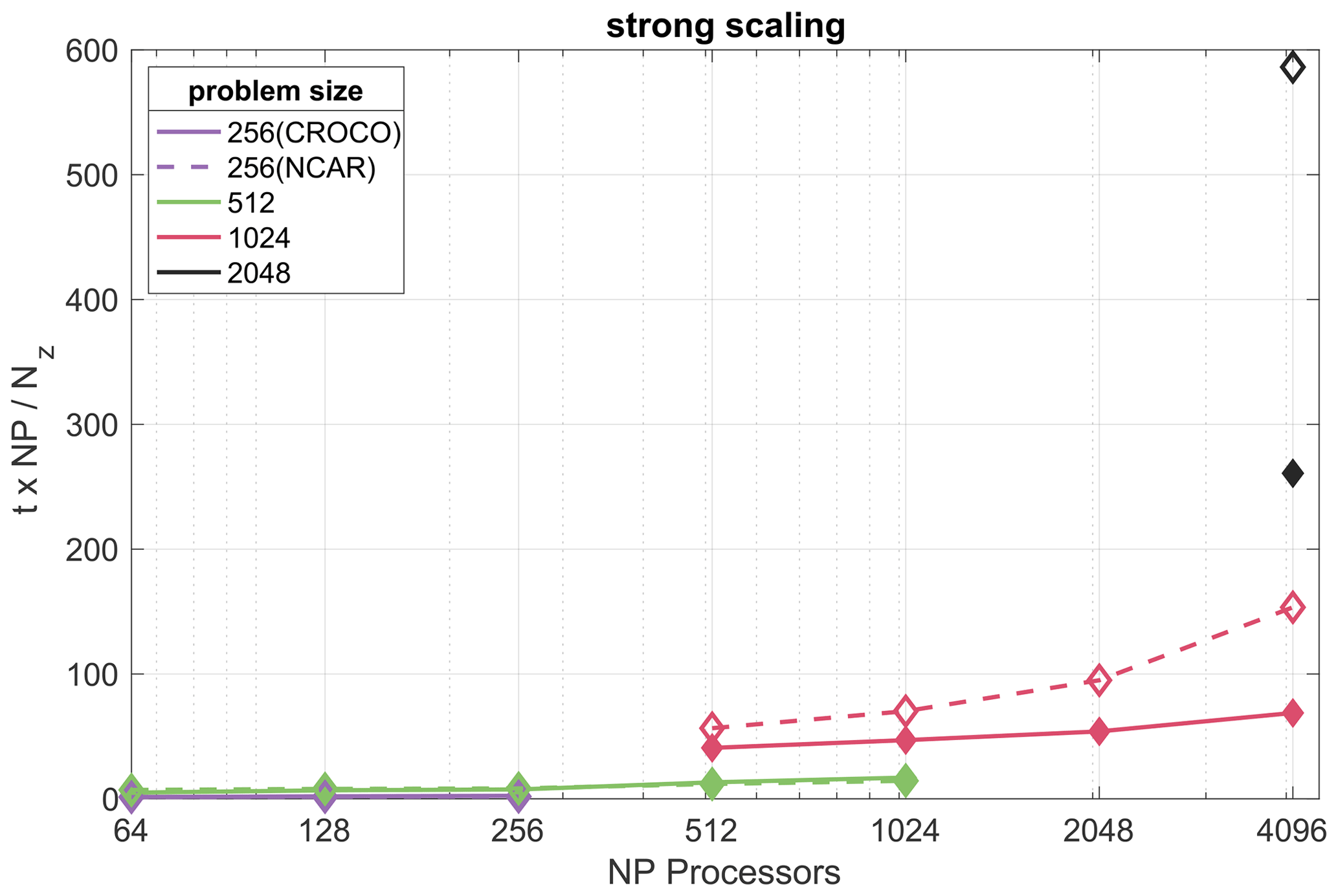
Figure 13Computational time per grid point per time step for different combinations of problem size for CROCO (solid) and NCAR-LES (dashed), as an example of strong scaling. NDTFAST = 200. (a) Purple lines and symbols problem size 2563. (b) Green lines and symbols 5123. (c) Red lines and symbols 10243. (d) Black symbol 20483.
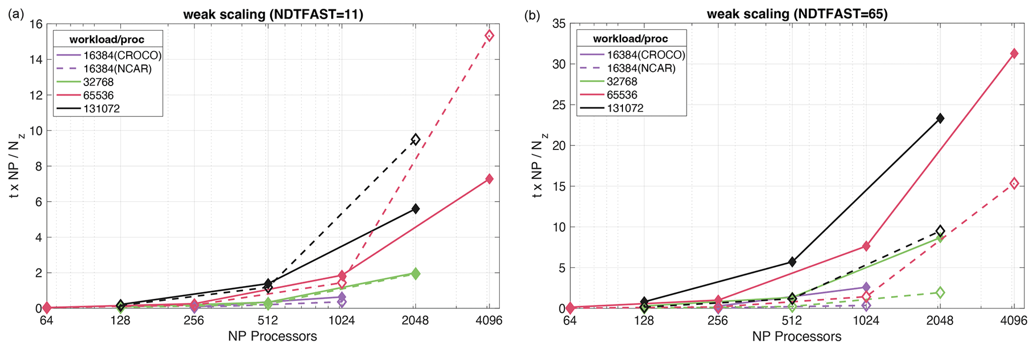
Figure 14Computational time per grid point for a fixed amount of work (i.e., same number of slow time steps and grid points) per processor (an example of weak scaling) with 11 fast (barotropic and pseudo-acoustic) time steps per slow (baroclinic) time step (a) and 65 fast time steps per slow time step (b).
In order to evaluate the performance of the ocean model CROCO with non-hydrostatic kernels, this paper uses NCAR-LES as a benchmark for comparison. The study begins with a comparison of several different LES versions, and then, because of their close agreement, only NCAR-LES is used elsewhere. Two comparison aspects of CROCO and NCAR-LES are simulation accuracy and computational efficiency.
In the accuracy tests, the effect of the explicit SGS parameterization, the second viscosity parameter, and the speed-of-sound parameter are varied to understand these key factors impacting simulation accuracy. Once these parameters are considered, the NCAR-LES results and the CROCO results are overall within expected variations. The simulated mean flows are very similar. The only notable differences are (1) that the CROCO surface velocity tends to be slightly higher, (2) that the CROCO surface temperature tends to be slightly lower, and (3) that the CROCO pycnocline entrainment is weaker. These effects are best explained by noting that CROCO's numerical diffusion is weaker than the explicit SGS plus implicit diffusion of the NCAR model. The NCAR runs have stronger internal waves (contributing no buoyancy flux when statistically steady) and less resolved turbulent mixing. There are other minor differences, but most of them are expected due to the different SGS parameterization and limited averaging windows. Overall, the differences between CROCO and the NCAR-LES are similar to the differences between three different LES codes. The only notable difference that may not be attributable to the SGS parameterization difference is that the NCAR model runs tend to produce more internal waves where higher stratification is present, a result that is also sensitive to the speed-of-sound setting in CROCO. As for the effect of the second (dilatation) viscosity parameter, increasing λ damps marginally unstable modes but allows only moderately larger time steps. Decreasing the speed of sound from 202 to 3 m s−1 allowed a factor of 5 times faster simulations with negligible changes to the solution accuracy. However, this is a simulation-specific adjustment, and such a large reduction in the speed of sound is likely to have consequences in other simulated scenarios. A rough comparison between CROCO on a stretched vertical grid and NCAR-LES on a uniform grid finds that the stretched grid does not significantly magnify the model discrepancies in this setting.
In efficiency tests, based on the Cheyenne supercomputer platform, the difference between CROCO and NCAR-LES performance at weak and strong scaling on their computational parallelization and 2D decomposition was found. The strong scaling represents the computational time per grid point per time step for different combinations of processors for each problem size, and the weak scaling represents computational time per grid point for a fixed amount of work per processor. In both cases, the computational efficiency of CROCO and NCAR-LES per time step is comparable. The number of fast subcycle time steps in CROCO affects its efficiency, but it ranged from 2 times to half as expensive as NCAR-LES per time step. To sum up, CROCO and LES are comparable on their simulation accuracy and computational efficiency per time step.
However, in these idealized test cases where the advantages of a weak compressibility approach to realistic simulations (where CROCO has specialized capabilities) are unimportant, these capabilities limit the time step in CROCO to be 6 to 14 times smaller, depending on the strength of the forcing. CROCO optimizations are ongoing and will be documented in future publications; using the Runge–Kutta version of CROCO may allow approximately a doubling of time step length (Lemarié et al., 2015). Avoiding the fifth-order WENO scheme also makes CROCO faster, although with possibly larger dispersion errors. A new variant on the CROCO nonhydrostatic numerics (removing the need for solving non-hydrostatic modes at the free surface, which severely constrain the time step) is in prototype testing and should allow much faster simulations. The version of NCAR-LES used here can also be sped up by 10 %–15 % using a new Fourier transform package (MKL FFT).
The only simulation result difference between CROCO and NCAR-LES that was not attributable to the SGS parameterization differences is that NCAR-LES tends to produce slightly more internal waves. The CROCO solutions were found to be insensitive to the values of the second viscosity and the speed of sound over wide ranges. Therefore, an artificially large value of the second viscosity and an artificially small value of speed of sound were used to increase the time step stably and accurately, as long as the speed of sound is faster than the speed of the fastest process that needs to be properly simulated (this constraint will be eased with the new variant currently being tested). Overall, when the additional features of CROCO are needed (nesting, complex topography, free surface, etc.), these additional costs can be justified, while in idealized settings, in a rectangular domain with mathematically well-defined periodic boundary conditions, the NCAR-LES is faster at arriving at nearly the same result.
The latest CROCO ROMS code is available for download at http://croco-ocean.org (Auclair et al., 2024). The latest NCAR-LES model is available upon request to pps@ucar.edu. The versions of the code compared here are available at https://doi.org/10.5281/zenodo.8431670 (Fan et al., 2023a) and https://doi.org/10.5281/zenodo.8431732 (Fan et al., 2023b).
The simulation data underlying this paper are available from the permanent archive of the Brown Digital Repository at https://doi.org/10.26300/vpdb-v266 (Fan et al., 2023c).
XF, NS, QL, and BFK conceived the project. XF, NS, and QL ran the simulations. PM, FA, and PS contributed expertise on the CROCO and NCAR-LES models. All authors participated in the writing. XF organized the writing contributions. This project is XF's Master's degree project, and BFK is her advisor.
The contact author has declared that none of the authors has any competing interests.
Publisher's note: Copernicus Publications remains neutral with regard to jurisdictional claims made in the text, published maps, institutional affiliations, or any other geographical representation in this paper. While Copernicus Publications makes every effort to include appropriate place names, the final responsibility lies with the authors.
Baylor Fox-Kemper and Xiaoyu Fan and computing at Brown University were supported by the National Science Foundation (NSF) (grant no. 1655221). Time on Cheyenne was supplied by the Computational and Information Systems Laboratory at the National Center for Atmospheric Research (Computational and Information Systems Laboratory, 2019). Qing Li acknowledges support from the Center for Ocean Research in Hong Kong and Macau. The collaboration of Nobuhiro Suzuki has been supported by Innovation, Information & Biologisation-Fonds (I2B-Fonds). The comments of two anonymous reviewers greatly improved the clarity of the paper.
This research has been supported by the National Science Foundation Office of Integrative Activities no. 1655221.
This paper was edited by P. N. Vinayachandran and reviewed by two anonymous referees.
Auclair, F., Bordois, L., Dossmann, Y., Duhaut, T., Paci, A., Ulses, C., and Nguyen, C.: A non-hydrostatic non-Boussinesq algorithm for free-surface ocean modelling, Ocean Model., 132, 12–29, https://doi.org/10.1016/j.ocemod.2018.07.011, 2018. a, b
Auclair, F., Benshila, R., Capet, X., Debreu, L., Dumas, F., Jullien, S., and Marchesiello, P.: Coastal and Regional Ocean COmmunity model, https://www.croco-ocean.org/, last access: 8 May 2024. a
Bachman, S. D., Fox-Kemper, B., and Pearson, B.: A Scale-Aware Subgrid Model for Quasigeostrophic Turbulence, J. Geophys. Res.-Oceans, 122, 1529–1554, https://doi.org/10.1002/2016JC012265, 2017. a
Beets, C. and Koren, B.: Large-eddy simulation with accurate implicit subgrid-scale diffusion, Department of Numerical Mathematics Rep., NM-R9601, pp. 24, 1996. a
Borges, R., Carmona, M., Costa, B., and Don, W. S.: An improved weighted essentially non-oscillatory scheme for hyperbolic conservation laws, J. Comput. Phys., 227, 3191–3211, https://doi.org/10.1016/j.jcp.2007.11.038, 2008. a
Computational and Information Systems Laboratory: Cheyenne: HPE/SGI ICE XA System (Climate Simulation Laboratory), National Center for Atmospheric Research, Boulder, Colorado, https://doi.org/10.5065/D6RX99HX, 2019. a
Deardorff, J. W.: Stratocumulus-Capped Mixed Layers Derived from a Three-Dimensional Model, Bound.-Lay. Meteorol., 18, 495–527, https://doi.org/10.1007/BF00119502, 1980. a, b
Debreu, L., Auclair, F., Benshila, R., Capet, X., Dumas, F., Julien, S., and Marchesiello, P.: Multiresolution in CROCO (Coastal and Regional Ocean Community model), in: EGU General Assembly Conference Abstracts, EGU2016-15272-1, 2016. a
Fan, X., Fox-Kemper, B., Suzuki, N., Li, Q., Marchesiello, P., Auclair, F., Sullivan, P., and Hall, P.: CROCO code as used in “Comparison of the Coastal and Regional Ocean Community Model (CROCO) and NCAR-LES in Non-hydrostatic Simulations”, Zenodo [code], https://doi.org/10.5281/zenodo.8431670, 2023a. a, b
Fan, X., Fox-Kemper, B., Suzuki, N., Li, Q., Marchesiello, P., Auclair, F., Sullivan, P., and Hall, P.: NCAR-LES code as used in “Comparison of the Coastal and Regional Ocean Community Model (CROCO) and NCAR-LES in Non-hydrostatic Simulations”, Zenodo [code], https://doi.org/10.5281/zenodo.8431732, 2023b. a, b
Fan, X., Li, Q., Fox-Kemper, B., and Nobuhiro, S.: Data for Comparison of the coastal and regional ocean community model (CROCO) and NCAR-LES in non-hydrostatic simulations, Brown University Open Data Collection, Brown Digital Repository [data set], https://doi.org/10.26300/vpdb-v266, 2023c. a, b
Fox, D. G. and Orszag, S. A.: Pseudospectral approximation to two-dimensional turbulence, J. Comput. Phys., 11, 612–619, https://doi.org/10.1016/0021-9991(73)90141-1, 1973. a
Fox-Kemper, B., Adcroft, A., Boening, Claus W., C. W., Chassignet, E. P., Curchitser, E., Danabasoglu, G., Eden, C., England, M. H., Gerdes, R., Greatbatch, R. J., Griffies, S. M., Hallberg, R. W., Hanert, E., Heimbach, P., Hewitt, H. T., Hill, C. N., Komuro, Y., Legg, S., Le Sommer, J., Masina, S., Marsland, S. J., Penny, S. G., Qiao, F., Ringler, T. D., Treguier, A. M., Tsujino, H., Uotila, P., and Yeager, S. G.: Challenges and Prospects in Ocean Circulation Models, Front. Mar. Sci., 6, 65, https://doi.org/10.3389/fmars.2019.00065, 2019. a, b
Haidvogel, D. B., Arango, H., Budgell, W. P., Cornuelle, B. D., Curchitser, E., Di Lorenzo, E., Fennel, K., Geyer, W. R., Hermann, A. J., Lanerolle, L., Levin, J., McWilliams, J. C., Miller, A. J., Moore, A. M., Powell, T. M., Shchepetkin, A. F., Sherwood, C. R., Signell, R. P., Warner, J. C., and Wilkin, J.: Ocean forecasting in terrain-following coordinates: Formulation and skill assessment of the Regional Ocean Modeling System, J. Comput. Phys., 227, 3595–3624, 2008. a
Lemarié, F., Debreu, L., Madec, G., Demange, J., Molines, J.-M., and Honnorat, M.: Stability constraints for oceanic numerical models: implications for the formulation of time and space discretizations, Ocean Model., 92, 124–148, 2015. a
Li, Q. and Fox-Kemper, B.: Assessing the Effects of Langmuir Turbulence on the Entrainment Buoyancy Flux in the Ocean Surface Boundary Layer, J. Phys. Oceanogr., 47, 2863–2886, https://doi.org/10.1175/JPO-D-17-0085.1, 2017. a, b, c, d
Li, Q. and Fox-Kemper, B.: Anisotropy of Langmuir Turbulence and the Langmuir-Enhanced Mixed Layer Entrainment, Phys. Rev. Fluids, 5, 013803, https://doi.org/10.1103/PhysRevFluids.5.013803, 2020. a
Lilly, D. K.: On the numerical simulation of buoyant convection, Tellus, 14, 148–172, https://doi.org/10.3402/tellusa.v14i2.9537, 1962. a, b
Marchesiello, P., Auclair, F., Debreu, L., McWilliams, J., Almar, R., Benshila, R., and Dumas, F.: Tridimensional nonhydrostatic transient rip currents in a wave-resolving model, Ocean Model., 163, 101816, https://doi.org/10.1016/j.ocemod.2021.101816, 2021. a, b
Maronga, B., Gryschka, M., Heinze, R., Hoffmann, F., Kanani-Sühring, F., Keck, M., Ketelsen, K., Letzel, M. O., Sühring, M., and Raasch, S.: The Parallelized Large-Eddy Simulation Model (PALM) version 4.0 for atmospheric and oceanic flows: model formulation, recent developments, and future perspectives, Geosci. Model Dev., 8, 2515–2551, https://doi.org/10.5194/gmd-8-2515-2015, 2015. a
Marshall, J., Hill, C., Perelman, L., and Adcroft, A.: Hydrostatic, quasi-hydrostatic, and nonhydrostatic ocean modeling, J. Geophys. Res.-Oceans, 102, 5733–5752, 1997. a, b
McWilliams, J. C.: A uniformly valid model spanning the regimes of geostrophic and isotopic, stratified turbulence: Balanced turbulence, J. Atmos. Sci., 42, 1773–1774, 1985. a
McWilliams, J. C., Sullivan, P. P., and Moeng, C.-H.: Langmuir Turbulence in the Ocean, J. Fluid Mech., 334, 1–30, https://doi.org/10.1017/S0022112096004375, 1997. a
Mellor, G. L.: Users guide for a three dimensional, primitive equation, numerical ocean model, Program in Atmospheric and Oceanic Sciences, Princeton University Princeton, NJ, 1998. a
Moeng, C.-H.: A Large-Eddy-Simulation Model for the Study of Planetary Boundary-Layer Turbulence, J. Atmos. Sci., 41, 2052–2062, https://doi.org/10.1175/1520-0469(1984)041<2052:ALESMF>2.0.CO;2, 1984. a, b, c, d, e
Monin, A. and Obukhov, A.: Basic laws of turbulent mixing in the surface layer of the atmosphere, Contrib. Geophys. Inst. Acad. Sci. USSR, 151, e187, 1954. a
Orszag, S. A.: On the Elimination of Aliasing in Finite-Difference Schemes by Filtering High-Wavenumber Components, J. Atmos. Sci., 28, 1074–1074, https://doi.org/10.1175/1520-0469(1971)028<1074:OTEOAI>2.0.CO;2, 1971. a
Raasch, S. and Schröter, M.: PALM – A Large-Eddy Simulation Model Performing on Massively Parallel Computers, Meteorol. Z., 10, 363–372, https://doi.org/10.1127/0941-2948/2001/0010-0363, 2001. a, b
Ramadhan, A., Wagner, G., Hill, C., Campin, J.-M., Churavy, V., Besard, T., Souza, A., Edelman, A., Ferrari, R., and Marshall, J.: Oceananigans.Jl: Fast and Friendly Geophysical Fluid Dynamics on GPUs, J. Open Source Softw., 5, 2018, https://doi.org/10.21105/joss.02018, 2020. a, b
Skitka, J., Marston, J. B., and Fox-Kemper, B.: Reduced-Order Quasilinear Model of Ocean Boundary-Layer Turbulence, J. Phys. Oceanogr., 50, 537–558, https://doi.org/10.1175/JPO-D-19-0149.1, 2020. a
Smagorinsky, J.: General circulation experiments with the primitive equations: I. The basic experiment, Mon. Weather Rev., 91, 99–164, 1963. a
Sullivan, P., McWilliams, J., and Moeng, C.: A subgrid-scale model for large-eddy simulation of planetary boundary-layer flows, Bound.-Lay. Meteorol., 71, 247–276, https://doi.org/10.1007/BF00713741, 1994. a, b, c, d, e
Sullivan, P., McWilliams, J., and Moeng, C.: A grid nesting method for large-eddy simulation of planetary boundary-layer flows, Bound.-Lay. Meteorol., 80, 167–202, https://doi.org/10.1007/BF00119016, 1996. a
Sullivan, P. P. and Patton, E. G.: A highly parallel algorithm for turbulence simulations in planetary boundary layers: Results with meshes up to 2048 3, in: 18th Symposium on Boundary Layers and Turbulence, 2008. a, b, c
Sullivan, P. P. and Patton, E. G.: The Effect of Mesh Resolution on Convective Boundary Layer Statistics and Structures Generated by Large-Eddy Simulation, J. Atmos. Sci., 68, 2395–2415, https://doi.org/10.1175/JAS-D-10-05010.1, 2011. a, b
Verstappen, R.: How Much Eddy Dissipation Is Needed to Counterbalance the Nonlinear Production of Small, Unresolved Scales in a Large-Eddy Simulation of Turbulence?, Comput. Fluids, 176, 276–284, https://doi.org/10.1016/j.compfluid.2016.12.016, 2018. a
Wedi, N. P. and Smolarkiewicz, P. K.: A framework for testing global non-hydrostatic models, Q. J. Roy. Meteor. Soc., 135, 469–484, 2009. a
Wicker, L. J. and Skamarock, W. C.: Time-Splitting Methods for Elastic Models Using Forward Time Schemes, Mon. Weather Rev., 130, 2088–2097, https://doi.org/10.1175/1520-0493(2002)130<2088:TSMFEM>2.0.CO;2, 2002. a
Each profile is an average of 21 samples taken every 1/40 (about 25 min) of the inertial period during t= 4.7 to 13.6 h. At each given time, the normalized profiles are computed using the characteristic scales at that time. Then, the final profiles are made by averaging these normalized profiles. The time window is kept short, about 9 h, because the simulated flow is not in a statistically steady state due to mixed-layer deepening and entrainment. In all simulations, the boundary-layer thickness reaches the initial mixed-layer thickness within 4 h from t=0 s when the flow has no motion.
Here, for notational simplicity, we use a positive value when energy is coming into the water.
The length scale Δe is independent of the flow. Therefore, an arbitrary value may be used. Here we arbitrarily use Δe=1 m.
The factor 4.5 is an empirical non-dimensional coefficient. Equation (6) is related to the standard thickness of the Ekman layer derived, assuming a constant vertical eddy viscosity. Here, however, we relate the wind-driven boundary-layer thickness to the surface energy flux because the eddy viscosity does not have to be vertically uniform but is still roughly related to the surface energy flux.
When the wind energy mixes the surface water very well and thereby significantly distracts the available potential energy due to the surface cooling, it may be more appropriate to use instead in the second term.
That is, the normalized-buoyancy frequency of the pycnocline tends to be smaller for the CROCO runs, while the dimensional N2 of the pycnocline is the same for both NCAR and CROCO runs. This is a result of a slightly larger in the CROCO runs, which leads to a larger UE, a deeper zw, a smaller zw−zp, a larger Eb, and a larger ΓN.
Each profile is an average of 21 samples taken every 1/40 of the inertial period during t= 4.7 to 13.6 h.
In Sullivan and Patton (2008), a different scaling for horizontal effort was used because the NCAR-LES is pseudo-spectral: Mx = Nx logNx, with Nx the number of grid points in the x direction or a similar formula for the y direction. This scaling is not used here because CROCO is not pseudo-spectral.