LB-SCAM: a learning-based method for efficient large-scale sensitivity analysis and tuning of the Single Column Atmosphere Model (SCAM)

The single-column model, with its advantages of low computational cost and fast execution speed, can assist users in gaining a more intuitive understanding of the impact of parameters on the simulated results of climate models. It plays a crucial role in the study of parameterization schemes, allowing for a more direct exploration of the influence of parameters on climate model simulations. In this paper, we employed various methods to conduct sensitivity analyses on the 11 parameters of the Single Column Atmospheric Model (SCAM). We explored their impact on output variables such as precipitation, temperature, humidity, and cloud cover, among others, across five test cases. To further expedite experimentation, we utilized machine learning methods to train surrogate models for the aforementioned cases. Additionally, three-parameter joint perturbation experiments were conducted based on these surrogate models to validate the combined parameter effects on the results. Subsequently, targeting the sensitive parameter combinations identified from the aforementioned experiments, we further conducted parameter tuning for the corresponding test cases to minimize the discrepancy between the results of SCAM and observational data. Our proposed method not only enhances model performance but also expedites parameter tuning speed, demonstrating good generality at the same time.

1 Introduction

Earth system models (ESMs) are important tools to help people recognize and understand the effects of global climate change. The Community Earth System Model (CESM) is one of the most popular and widely used ESMs, which includes atmosphere, ocean, land, and other components (Hurrell et al., 2013). Of these components, the Community Atmosphere Model (CAM) (Neale et al., 2010; Zhang et al., 2018) plays an important role as the atmospheric component of CESM. Most of the physics parts in CAM are described as parameterization schemes with tunable parameters that are often derived from limited measurements or theoretical assumptions. However, since CAM needs to simulate all the grids, it takes a long time and a large number of resources to run. Thus, the Single Column Atmospheric Model (SCAM) (Bogenschutz et al., 2013; Gettelman et al., 2019) has been developed as a cheaper and more efficient alternative model for the purpose of tuning physics parameters (Bogenschutz et al., 2020). And in order to tune the parameters, we often need to conduct a large number of simulated experiments. This will result in significant computational costs. Meanwhile, SCAM only needs to simulate one single column, and only one process is required for each run of one case to complete the simulation. As a result, SCAM becomes a natural tool for studying how the parameters would affect the uncertainty in the modeling results, and the use of SCAM for large-scale experiments is more practicable due to its advantage of lower requirements for computing resources.

Climate models are among some of the most complex models; we can abstract it as a function with numerous independent and dependent variables, and there is uncertainty between them. In research, identifying independent variables that significantly affect the dependent variable can help to quickly understand the relationship between them. Sensitivity analysis (SA) is an important method used to achieve this purpose (Saltelli et al., 2010). A rich set of numerical and statistical methods have been developed over the years to study the uncertainty in models in many different domains, ranging from natural sciences and engineering to risk management in finance and social sciences (Saltelli et al., 2008). SA of climate models generally involves two steps: generating representative samples with different values of parameters using a specific sampling method and exploring and identifying the sensitivity metrics between the model output and the parameters to study. Typical approaches include the Morris one-at-a-time (MOAT) method that uses the Morris sampling scheme (Morris, 1991), which generates samples uniformly and has a good computing efficiency, and the variance-based Sobol method that generally requires a lot more samples to achieve a good coverage of the space (Sobol, 1967; Saltelli, 2002). Other similar ideas to achieve a good representation of the sample space with a quasi-random sequence include the quasi-Monte Carlo (QMC) (Caflisch, 1998) and Latin hypercube (LHC) (McKay et al., 2000) sampling methods. The samples obtained from these sampling methods can be combined with sensitivity analysis methods such as Sobol (Sobol, 1967), high-dimensional model representation (HDMR, Li et al., 2010), a random balance design Fourier amplitude sensitivity test (RBD-FAST, Goffart et al., 2015), and a delta moment-independent measure (Plischke et al., 2013). This allows for an assessment of the individual parameter impacts on global outcomes, as well as the interrelationships between pairs, i.e., second-order sensitivity.

However, in practical applications, the number of parameters that need to be tuned is often more than two. When tuning multiple parameters, considering the intricate connections between them, there will inevitably be mutual influences. Just like the three-body problem in astronomy, when simultaneously tuning three or more parameters, the complexity will be much greater than tuning each of these three parameters individually. Therefore, whether the sensitivity analysis results obtained based on existing methods can accurately provide us with the optimal combination of multiple parameters is a question worth considering. Investigating the overall impact of combined parameters on the system output is worthy of further exploration. This holds true for climate models as well.

After we have determined the combination of parameters to be tuned, we can then tune them to improve the performance of the model. With a general goal of achieving modeling results as close to the observations as possible, we can apply different optimization methods, such as the genetic algorithm (GA) (Mitchell, 1996), differential evolution (DE) (Storn and Price, 1997), and particle swarm optimization (PSO) (Kennedy and Eberhart, 2002), to identify the most suitable set of parameters.

Continuous efforts have been put into the tunable parameters in climate models, especially for the their physics parameterization schemes (Yang et al., 2013; Guo et al., 2015; Pathak et al., 2021). Yang et al. (2013) analyzed the sensitivity of nine parameters in the ZM deep convection scenario for CAM5 and used the simulated stochastic approximation annealing method to optimize the precipitation performance in different regions by zoning. Zou et al. (2014) conducted a sensitivity analysis for seven parameters in the MIT–Emanuel cumulus parameterization scheme in RegCM3. The precipitation optimization process for the CORDEX East Asia domain was carried out using the multiple very fast simulated annealing method.

For all the stages mentioned above, the computing cost of running the model becomes a major constraining factor that stops us from exploring more samples and identifying more optimal solutions. People sometimes use surrogates (such as a generalized linear model – GLM; Nelder and Wedderburn, 1972) instead of the actual model to further reduce the computing cost. For example, the study of the sensitivity of simulated shallow cumulus and stratocumulus clouds to the tunable parameters of the subnormal uniform cloud layer (CLUBB) (Guo et al., 2015) investigated the sensitivity of 16 specific parameters using the QMC sampling method and GLM as a surrogate, with experiments on three different cases (BOMEX, RICO, and DYCOMS-II RF01). A key problem to consider for the SA stage is to achieve a balance between the accuracy and economy of computing (Saltelli et al., 2008). Another study (Pathak et al., 2021) used the single-column case ARM97 to explore eight parameters related to the cloud processes, with Sobol as the sampling method and spectral projection (SP) and basis pursuit denoising (BPDN) as the surrogate model. In an ideal case, a more thorough study of the parameters that can provide more concrete guidance for the parameter selection would require a joint SA and tuning of different single-column cases, as well as a combinational study of the most sensitive parameters. There are toolkits such as PSUADE (Tong, 2016), DAKOTA (Dalbey et al., 2021), and STATA (Harada, 2012) that can implement SA and tuning. These software tools have made remarkable contributions to advancing the development of generic frameworks. However, with the progress of high-performance computing, usability and ease of deployment have become crucial aspects for existing application scenarios. Particularly, in recent years, rapid advancements in fields like machine learning have made it meaningful to leverage machine learning methods to accelerate research progress.

In this paper, to facilitate researchers in better utilizing SCAM and to support a more efficient and convenient parameter tuning for the physical schemes in SCAM, we propose a learning-based method, LB-SCAM, for efficient large-scale SA and tuning. In summary, our proposed LB-SCAM mainly makes the following contributions.

1. We selected 11 parameters from three different physical schemes in SCAM, sampled them within a certain range, and utilized machine learning methods to train surrogate models for the response of model outputs to parameter variations. We then selected five typical cases from SCAM and trained individual surrogate models for each of them. This further enhances the efficiency of conducting large-scale parameter testing for SCAM.

2. With the samples obtained in the previous step, we conducted sensitivity analyses using five typical sensitivity analysis methods to assess the impact of these 11 parameters on four output variables in SCAM. Additionally, based on the surrogate models trained in the previous step, we conducted single-parameter and three-parameter joint perturbation experiments separately. This allowed us to identify, for each case, the most sensitive combination of three parameters.

3. Building upon the first two steps, we further conducted a parameter optimization process for the mentioned cases and variables. Additionally, we delved deeper into the patterns observed in the total precipitation (PRECT) variable. This exploration included examining the distribution patterns in the three-dimensional parameter space and identifying distinct characteristics among the various cases.

Using our proposed LB-SCAM, we conducted an extensive set of SA and tuning experiments for five cases of SCAM, targeting precipitation performance. In addition to SA analysis, which provides sensitivity evaluation of each single parameter, we were able to study the sensitivity of combinations of three, four, or even five arbitrary parameters. During the tuning stage, our improved optimization scheme (targeting the same parameters) resulted in a 24.4 % increase in the accuracy of precipitation output compared to control experiments. Furthermore, it achieved a more than 50 % reduction in computing cost compared to using only the optimization algorithm.

2 Enabling a workflow of SA and parameter tuning

2.1 Model description

This paper focuses on the single-column model of the atmospheric model CAM5, i.e., SCAM5 (Bogenschutz et al., 2012), extracted from CESM version 1.2.2, one of the two versions that are efficiently supported on the Sunway TaihuLight Supercomputer (Fu et al., 2016). Our research in this paper is mainly based on five typical cases in SCAM5, as shown in Table 1. Among the five cases, two cases are located in the Southern Great Plains, which mainly study land convection. The other three cases are located in the tropics and mainly study tropical convection (Thompson et al., 1979; Webster and Lukas, 1992; May et al., 2008).

Table 1 The five typical SCAM cases studied in this paper.

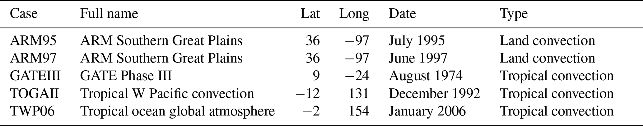
Table 2 The inclusion of variables in the IOP files of the SCAM cases studied in this paper.

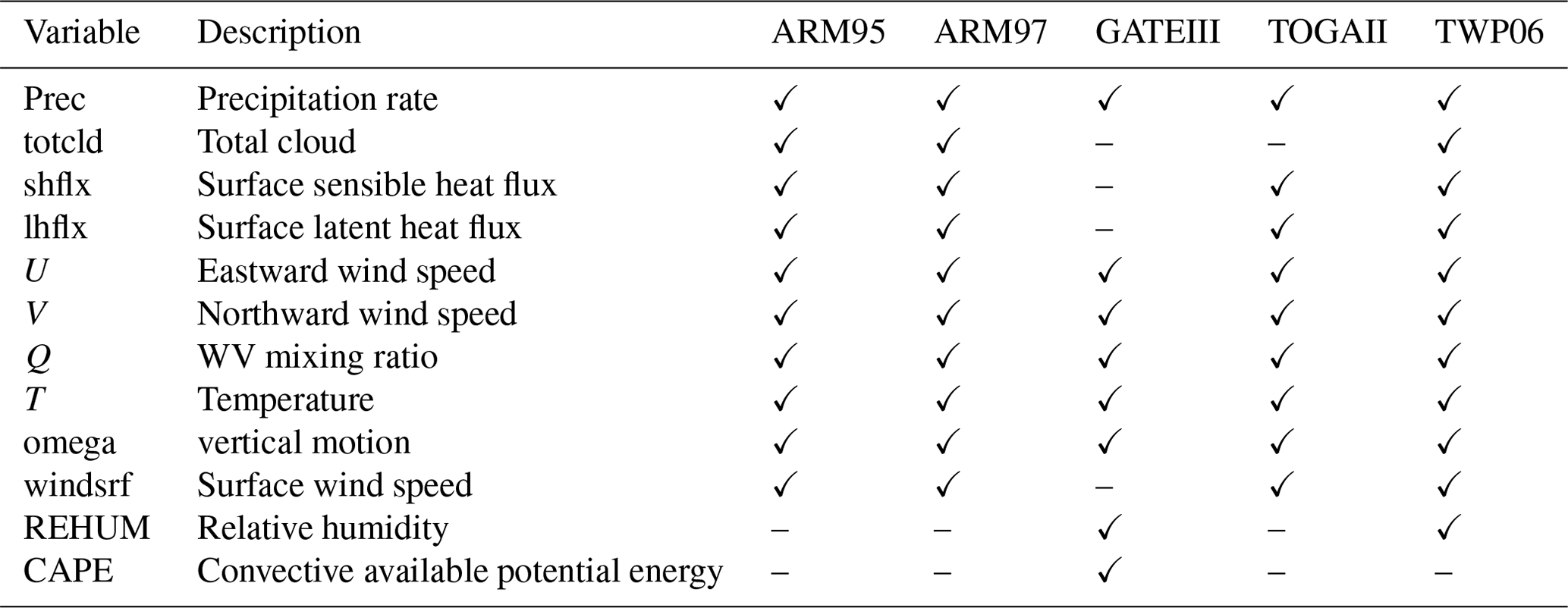
Table 3 The variables under study in this paper and their respective meanings.

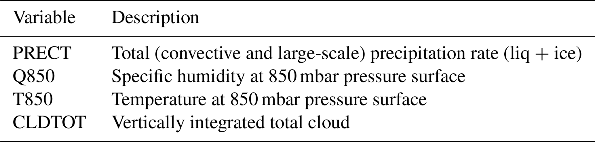
Table 4 List of parameters in the framework that can be tuned and applied to the experiment.

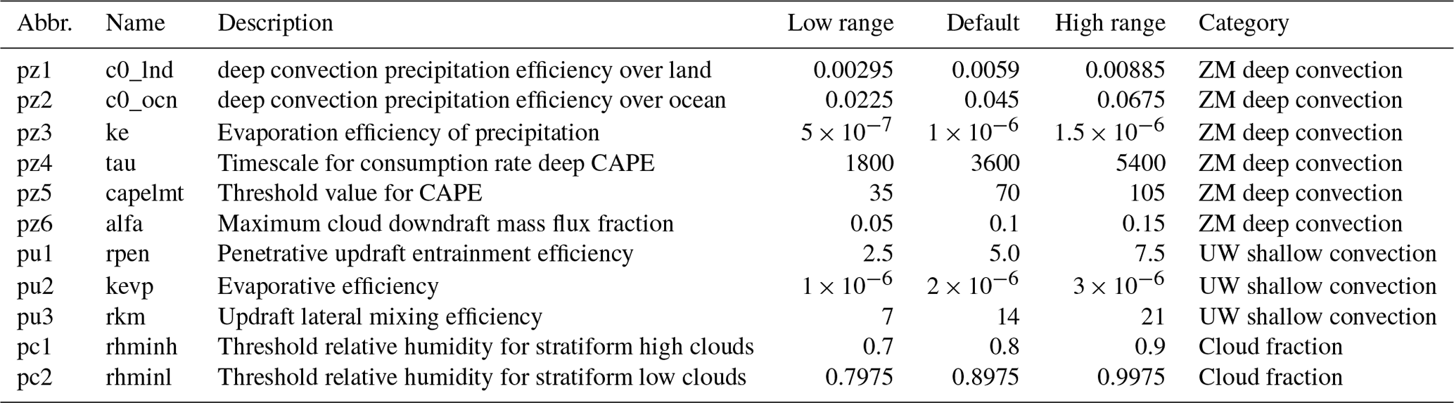
As shown in Tables 2 and 3, the number of observations included in the IOPs (intensive observation periods, Gettelman et al., 2019) file varies from case to case. In order to explore a joint parametric sensitivity analysis and tuning across all the five cases, we pick the intersection of the data owned by these cases, PRECT, Q850, T850, and CLDTOT, as the main research subject. The parameters listed in Table 4 are the main study targets (Qian et al., 2015) in this paper and the ones tested in the workflow. The parameters are selected from the ZM deep convection scheme (Zhang, 1995), the UW shallow convection scheme (Park, 2014), and cloud fraction (Gettelman et al., 2008). In the experiments in this paper, the lower and upper bounds of each parameter are 50 % and 150 % of the default value, respectively. For parameters with physical constraints, such as cldfrc_rhminh and cldfrc_rhminl, the values are ratios, so they are not more than 1.

In the original version of SCAM, only some of the parameters to be studied are tunable, while the rest are hard-coded in the model. To improve the flexibility of the model so that the 11 parameters we want to study are tunable, we have modified the source code of the model to support the tuning and study of a wider range of parameters. The corresponding Fortran source code and the XML documentation are also modified accordingly.

2.2 The workflow of sampling, SA, and parameter tuning

The submission of assignments and the collection of results are important issues when carrying out a large number of model experiments at the same time. Prior to conducting the experiments, the user is often presented with a broad set of boundaries of the parameters to be tuned, and the specific configuration of each experiment has to be decided in detail according to these ranges of values. After a large number of experiments have been completed, as the output of SCAM is stored in binary files in NetCDF format, the precipitation variables we want to study need to be extracted from a large number of output files in order to proceed to the next step. It is therefore necessary to provide the researcher with an automated experiment diagnosis process. In general, which parameters to tune and how to tune them are questions that deserve our attention.

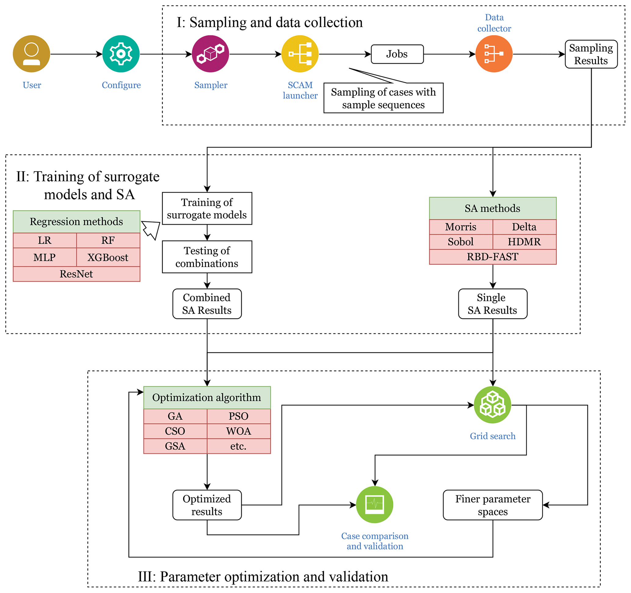
Figure 1 The overall workflow of the proposed method. Part I involves sampling and collecting results from parallel instances. In Part II, traditional SA methods are utilized to derive sensitivities of individual parameters, while simultaneously reusing the samples to develop learning-based surrogate models. By combining these surrogate models, we can then perform joint sensitivity analysis of a set of parameters. Guided by the SA results from Part II, Part III conducts parameter tuning, also using the surrogate models. The SCAM launcher, the data collector, and the jobs therein represent the batch execution of the SCAM cases, which is further explained in Fig. 2.

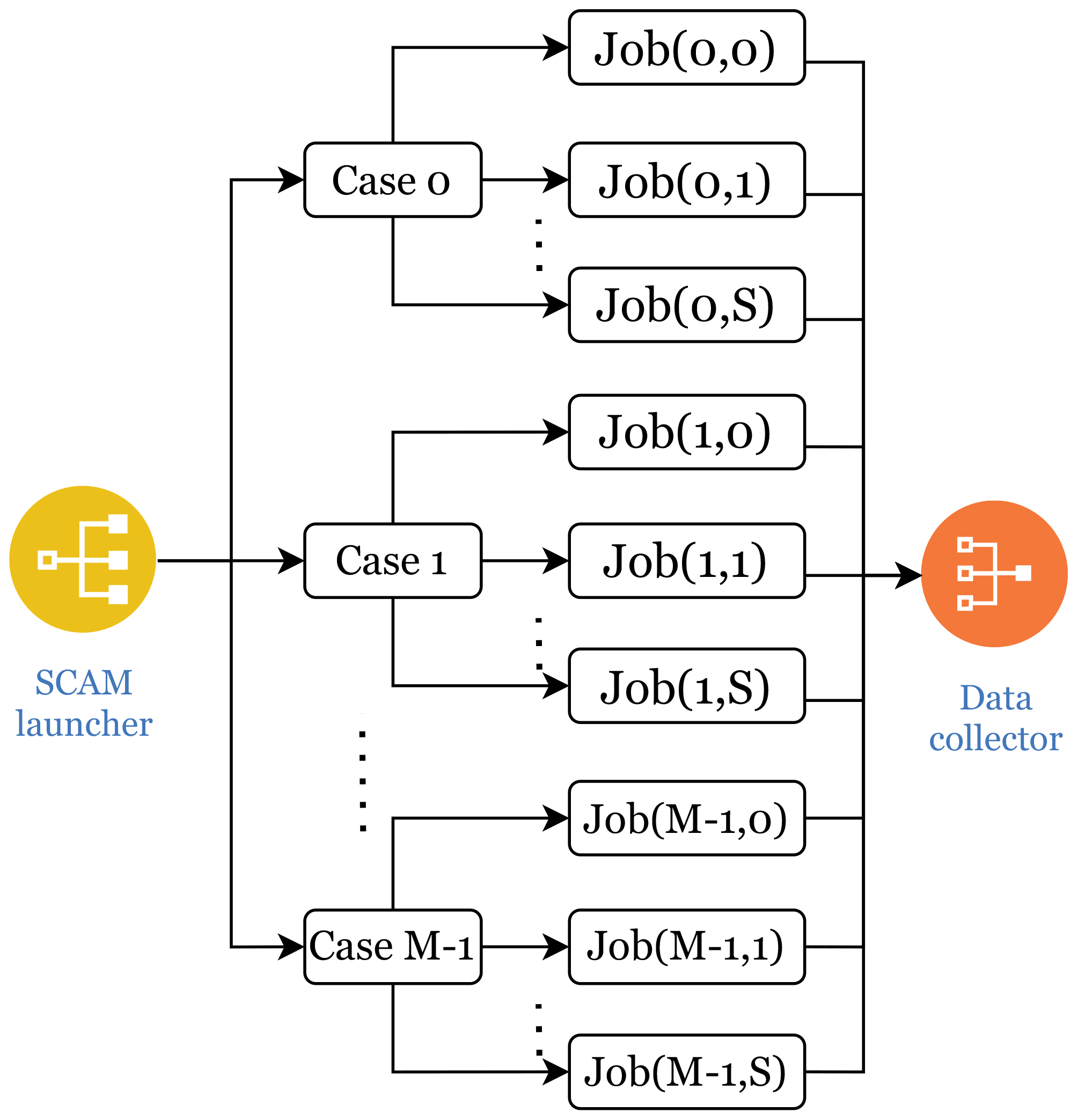
Figure 2 A detailed parallelism schematic is provided for running a large number of instances of multiple cases simultaneously. In this process, the launcher simultaneously initiates the required SCAM tasks, while the data collector gathers the results of their runs.

Based on the above needs, we have designed the SCAM parameter sampling, SA, tuning and analysis workflow. We integrate the collection and processing script for the post-sampling results. It supports a fully automated parameter tuning and diagnostic analysis process, a large number of concurrent model tests, and the search for the best combination of parameter values for SCAM performance within a given parameter space. Also, with the help of the training surrogate model, more parameter fetches can be tested in less time. The simulation results of the real model will be used as validation. This will further accelerate the degree of automation of scientific workflows (Guo et al., 2023) and thus accelerate conducting research in this area of Earth system models.

The overview of the whole scientific workflow is shown in Fig. 1. In order to make full use of computing resources and complete the sampling process as soon as resources allow, the proposed method supports parallel sampling processes, as shown in Fig. 2. Since SCAM is a single-process task and the computation time per execution is also short, it is feasible to execute a large batch of SCAM instances during the sampling stage.

Specifically for the application scenario in this paper, the execution process of the workflow is as follows.

1. Sampling and data collection (shown as Part I in Fig. 1). In this part, our tool generates the sequence of samples to investigate in the sampling step. Our tool currently supports the Sobol sequence, which can later be used by the Sobol, delta (Plischke et al., 2013), HDMR (Li et al., 2010), and RBD (Plischke et al., 2013) SA methods, as well as the Morris sampling sequence, which can later be used by the MOAT method (Morris, 1991). Users are suggested to adjust the size of the sequence according to the currently available computational resources. As the results of this step will be used as the training set for generating the surrogate model, users are encouraged to run a large batch when parallel resources are available to improve the performance of the resulting surrogate model. The process of launching the parallel cases and collecting the results is handled by the SCAM launcher and collector.

2. Surrogate model training and sensitivity analysis (shown as Part II in Fig. 1). Based on the sampling results from the Morris or the Sobol sequence, we integrate existing methods, such as MOAT, Sobol, delta, HDMR, and RBD, to achieve their individual evaluations of each single parameter's sensitivity, as well as a comparison result of these methods. We also use the sampling results of the Saltelli sequence and the Morris sequence to train regression including neural network (NN)-based surrogate models. In this section, different regression methods are used to compare their fits and the best fitting method to train the final surrogate model. With the efficiency to project a result in seconds rather than minutes, we can apply it for evaluation of sensitivities of a combination of multiple parameters.

3. Parameter tuning and validation (shown as Part III in Fig. 1). With the NN-based surrogate model to cover expanded search space with less time, we also propose an optimization method that combines grid searches by the surrogate model, which achieves better results with less computing time. The results of parameter tuning are then validated by running real SCAM cases. In addition, at the very end, we perform a comparison on the optimization results between the joint optimization across five cases and the independent optimization of the five cases. Results demonstrate the correlation of different cases and the potential of performing grid-specific tuning in the future.

3 Methodology

3.1 Sampling of SCAM

As an important preprocedure, the sampling provides the basis for analysis of SA. It will generate a sequence of changing inputs and parameters to observe the corresponding change in the output. The different mathematical approach that we take to perform sampling would certainly affect the features that can be captured from the system.

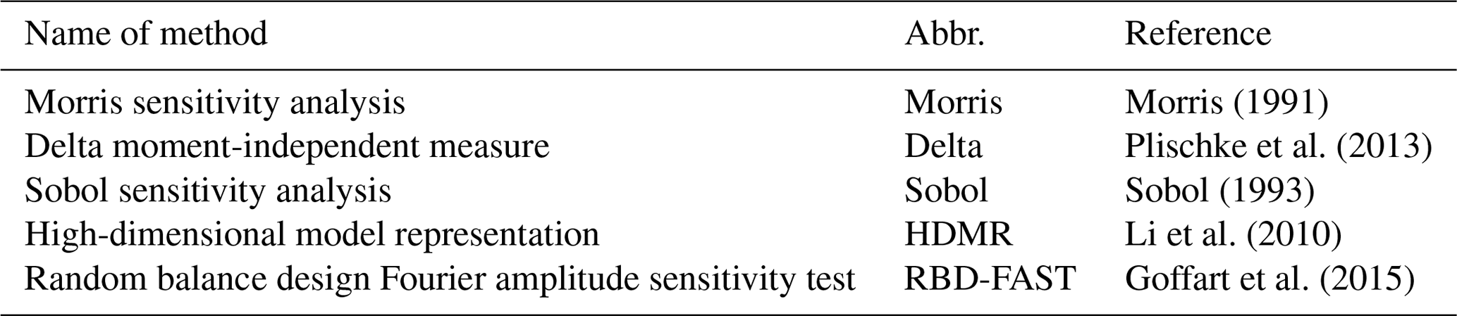
In our proposed workflow, we integrate both Morris and Saltelli for the sampling step in our tuning workflow, as both of them are still used in many climate-model-related SA studies (Pathak et al., 2021). The Morris sampling drives the MOAT SA module afterwards, while the Saltelli sampling drives four different SA modules (Sobol, delta, HDMR, and RBD-FAST) shown in Table 5.

After sampling, we will conduct a preliminary analysis of the sampled results to find out the proportion distribution in which the output results are better than the control trials under different values of each parameter. RMSE (root mean square error) will be used to measure the error between the output and the observed values and is defined as follows:

$$\begin{array}{}\text{(1)}& \mathrm{RMSE}=\sqrt{{\displaystyle \frac{\mathrm{1}}{N}}\sum _{i=\mathrm{1}}^N(y_i-{\widehat{y}}_i{)}^{\mathrm{2}}},\end{array}$$

where ${\widehat{y}}_i$ is the output at the ith time step of the current sample, while y_i is the observation at the corresponding time step.

Morris (1991)Plischke et al. (2013)Sobol (1993)Li et al. (2010)Goffart et al. (2015)

Table 5 SA methods integrated into the workflow and used as a cross-reference for the proposed method.

3.2 Training a learning-based surrogate model

A surrogate model is an important tool to speed up our large-scale parametric experiments. It can replace the running process of the original model, thus saving computing resources. The essence of training surrogate models for SCAM is a regression analysis problem. In this paper, we introduce the following regression methods to generate surrogate models. These include linear regression (LR, Yan et al., 2015), but also ensemble learning methods such as random forest (RF, Breiman, 2001) and eXtreme Gradient Boosting (XGBoost, Wang et al., 2018). Meanwhile, we also incorporate methods that use neural networks, such as multilayer perceptron (MLP, Tang et al., 2016) and residual network (ResNet, He et al., 2016; Shi et al., 2022).

In order to integrate the various regression analysis methods described above, we have designed an adaptive scheme to determine the method that best captures the nonlinear characteristics of the original model, thus obtaining the most appropriate surrogate model. To maintain an acceptable level of accuracy in the surrogate models, we opt to train separate models for each distinct SCAM case. The underlying assumption is that the model should learn the different patterns present in various SCAM case locations. Given that the Saltelli sequence of samples provides a comprehensive representation of the entire parameter space, we anticipate the model to perform well across different parameter combinations. Furthermore, we will conduct ablation experiments on the hyperparameters during the surrogate model training process to determine the most suitable hyperparameters, leading to better training.

3.3 Sensitivity analysis for a single parameter and combinations of parameters (enabled by the NN-based surrogate model)

The SA methods, similar to the climate model itself, have corresponding uncertainties. These methods provide the best estimation of each parameter's sensitivity based on their respective analytical principles. Therefore, each method may have its advantages and disadvantages in different ranges of parameter values.

As a result, in our workflow shown in Fig. 1, we choose to integrate multiple SA methods, including the ones that can be built on the Sobol sequence, such as delta, HDMR, RBD-FAST, and the Morris method, which is still used often for climate models due to its efficiency advantage. The integration of multiple methods enables us to better evaluate the uncertainty of different SA methods. As the sensitivity values calculated by the different methods are of different orders of magnitude, these sensitivities have been normalized using the min–max method for comparison purposes.

The parameters may interact with each other, and the effects of multiple parameters on the simulation results may be superimposed. Therefore, tuning multiple parameters generally has a more significant effect than tuning a single parameter. With the help of commonly used sensitivity analysis methods mentioned above, it is easy to obtain the sensitivity of individual parameters. However, in cases where we need to identify and tune a set of parameters in combination, both the sensitivity analysis and the tuning task would require a significantly increased level of computational resources.

An obvious benefit of using a surrogate model for training is its rapid computational speed. Since the model has been trained, the time required to output the surrogate results is significantly reduced. Therefore, we can explore as many combinations of parameters as possible with fewer computational resources. By applying the trained surrogate model, we can assess the maximum fluctuation in the output of each case when tuning different numbers of parameters simultaneously. This will aid in our decision-making process to determine the scale of meaningful and beneficial large-scale multi-parameter perturbation tests.

The utilization of the learning-based surrogate model, on the other hand, offers a more feasible solution to this problem. Since the surrogate model has a very short running time and almost does not require consideration of job queuing time, it enables the completion of a large-scale parameter experiment in a short time.

3.4 Parameter tuning enhanced with NN-based surrogate model and grid search

After the most sensitive sets of parameters have been found, the stage of optimization will begin.

In the optimization stage, on the basis of combining the existing optimization algorithms (such as GA, PSO, WOA), we propose an enhanced optimization method based on grid search. By using grid search, the search scope can be further narrowed before and during the call to the existing optimization algorithm so as to improve the efficiency of searching for better solutions. The process is as follows.

1. Determine the overall parameter space range for conducting the grid search based on the initial setup of the experiments.

2. The simulation output values corresponding to these grids are calculated using the surrogate model. Subsequently, the best-performing points are selected, and a new finer-grained search space is determined based on the aggregation of these points.

3. The optimization algorithm is executed in the newly defined space, and depending on the available computational resources, it is determined whether SCAM is invoked to compute in each iteration round. Additionally, the final results will also be validated by substituting them into SCAM.

4. If the same optimization result is obtained in three consecutive iterations or if there is less than a certain threshold of improvement compared to the last, the grid search operation of the first two steps is performed again, further reducing the search space, as illustrated in Algorithm 1. In this step, a new parameter space will be constructed with the position of the current best point at the center and the distance of each parameter from the last best point as the radius.

5. After refining the parameter search space, if the result remains unchanged, the optimization process can be considered complete, and SCAM can be run again using the derived parameters to verify the optimization results.

Algorithm 1 Optimization process combined with grid search.

if $Y_i-Y_{i-\mathrm{1}}<\mathit{ϵ}$ and $Y_{i-\mathrm{1}}-Y_{i-\mathrm{2}}<\mathit{ϵ}$ then

for j=1 to j=p do

if $x_{j,i}-|x_{j,i}-x_{j,i-\mathrm{3}}|>X_{j,\min }$ then

$X_{j,\min }^{*}=x_{j,i}-|x_{j,i}-x_{j,i-\mathrm{3}}|$

else

$X_{j,\min }^{*}=X_{j,\min }$

end if

if $x_{j,i}+|x_{j,i}-x_{j,i-\mathrm{3}}|<X_{j,\max }$ then

$X_{j,\max }^{*}=x_{j,i}+|x_{j,i}-x_{j,i-\mathrm{3}}|$

else

$X_{j,\max }^{*}=X_{j,\max }$

end if

end for

end if

Grid search.

return  $x_{j,i+\mathrm{1}}$ and Y_i+1

In Algorithm 1, Y_i is the value of the function in the ith iteration, ϵ is the threshold at which the results converge, p is the total number of parameters to be tuned, x_j,i represents the coordinates of x_j in the ith iteration, X_j denotes the maximum and minimum values initially set for x_j, and $X_j^{*}$ denotes the maximum and minimum values of x_j in the upcoming grid search. Note that if one of these coordinates is outside the initial parameter space, the original parameter space boundary will be used as the new boundary.

3.5 Case correlation analysis based on Pearson correlation coefficient

Following the end of the tuning process, we further perform a comparison study among different cases to derive valuable insights that would potentially lead to a physics module design that can accommodate the different features in different locations.

In our proposed method, the Pearson correlation coefficient method is used to measure the similarity between two cases (Schober et al., 2018). This coefficient is defined as the quotient of the covariance and standard deviation between two variables. By analyzing the similarity between the “optimal” parameters of each case, these cases can be clustered. In this process, we can explore whether for similar types of case, they may have similar responses to various parameters. This will also help us choose better parameter combinations when analyzing other cases, and even regional and global models, so as to achieve better simulations. The implementation is shown below.

1. Search the sensitive parameter sets for each output variable in each case.

2. For each case, the occurrence times of each parameter in the sensitive parameter combination are accumulated to obtain a variable of M dimension, where M is the number of parameters. For example, for a combination of three parameters, the vector can be expressed as (Value1, Value2, Value3).

3. The correlation between vectors of each case can be computed by the Pearson correlation coefficient method.

Through the above procedure, we can obtain the similarity of the set of sensitive parameters among the cases. The correlation between different cases can also be analyzed for the case of finding the optimal values in the same parameter space. After each case has found its optimal parameter values, this set of parameter values can also be represented by vectors. The same approach can be used to analyze the correlation between these vectors.

4 Experiments

4.1 Sampling of the SCAM cases

As mentioned earlier, the sampling scheme, which determines the set of points to represent the entire parameter space, is of essential importance for the following sensitivity analysis and parameter tuning steps. Considering the compatibility between the sampling methods and the SA methods, our platform includes both the Morris (driving the MOAT SA method) and the Sobol sampling scheme (driving the Sobol, delta, HDMR, and RBD-FAST SA methods). We use a total of 7680 samples, with 1536 samples for each of the five SCAM cases. Of these, half (i.e., 768 samples) are used for MOAT, while the remaining half are used for the Sobol sequence. In this part of the experiment, we use the job parallelism mechanism mentioned earlier in the text to execute these sample cases.

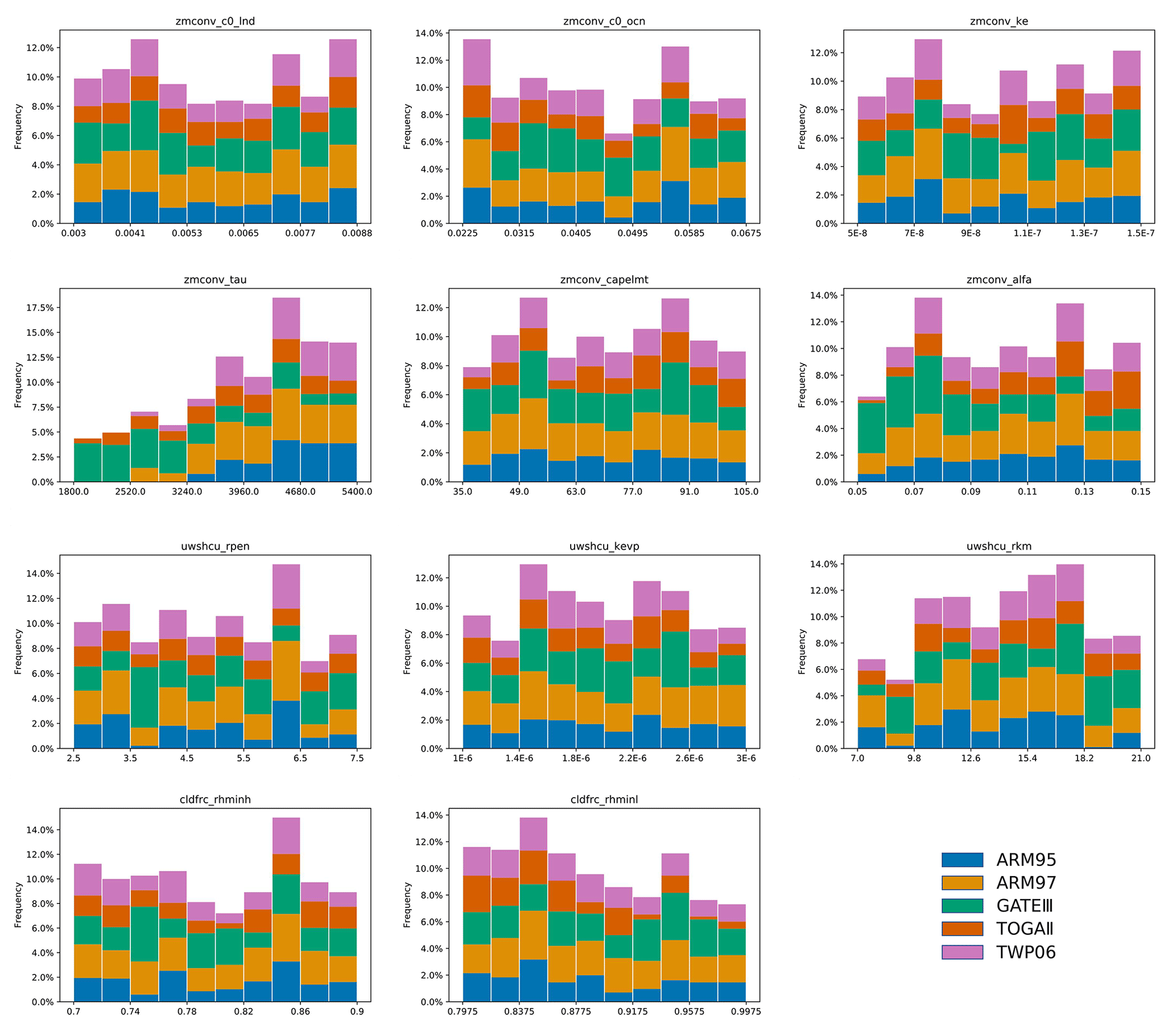
Figure 3 The proportion of sampled results where the output is better than the control experiments (i.e., experiments using default values) is shown on the x axis, which indicates the range of values for each parameter.

In our sampling, SA, and tuning study, we focus on the total precipitation output (PRECT). Figure 3 reflects the proportion of PRECT that outperforms the control experiments when each parameter is tuned from low to high in the range of values taken. From the results, we can see that for different cases there are differences in their response to parameter changes. Of particular interest is the distribution of pz4(tau). We can clearly see that for GATEIII, when the value of tau is small, there are more good outputs; however, for the other cases, when the value of tau is large, there are more outputs that perform well. It can also be seen from the proportion that tuning tau can lead to more good outputs. This is also in line with the results of our later experiments.

To further verify the conclusions here, we performed a single-parameter perturbation test on tau while keeping the other parameters as default values.

4.2 Training learning-based models for parameter tuning

After obtaining the sampling results, we can train the surrogate model for each of the five cases using the method presented in Sect. 3.2. The samples generated by the two sampling methods are combined to form the dataset on which we train our surrogate model. In other words, each case has 1536 samples, and all cases have a total of 7680 samples to participate in the training. We split the training and test set in an 8:2 ratio and use RMSE as the loss function during training.

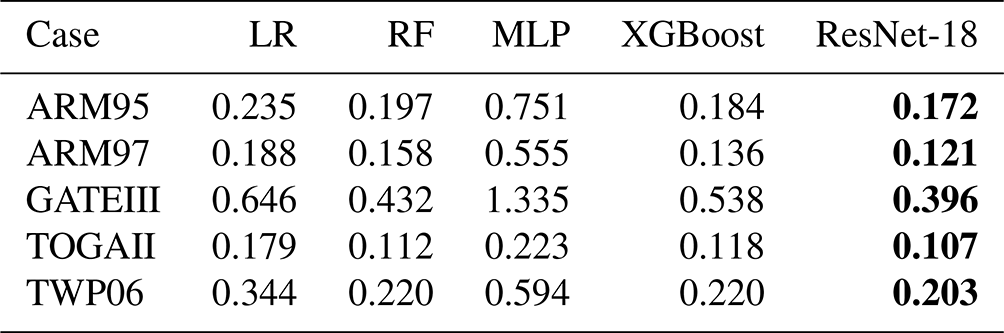
We trained surrogate models using five regression methods and used RMSE as a loss function to measure the training error. A comparison of the various methods is shown in Table 6. It can be seen that ResNet has the best performance on the five cases, and its error in the test set is lower than that of the other methods. Therefore, we will use the surrogate model trained by ResNet-18 for the following experiments. For the hyperparameters in training using ResNet-18, we also conduct ablation experiments to achieve better training results. The results of the ablation experiment indicate that using a learning rate of 0.01 and a batch size of 32 is appropriate.

Table 6 Comparison of errors during training using various methods. RMSE is used as the loss function. The errors are from test sets. The most effective method is represented in bold.

4.3 Single-parameter sensitivity analysis across different cases

After sampling, five SA methods listed in Table 5 are used to compute the sensitivity of these parameters to the PRECT, Q850, T850, and CLDTOT output. In addition, for the surrogate models we trained, we also adopted the single-parameter perturbation method to test their sensitivities. Heat maps are used to characterize the sensitivities of each parameter. As can be seen from Fig. 4, there are differences in the results obtained from different SA methods.

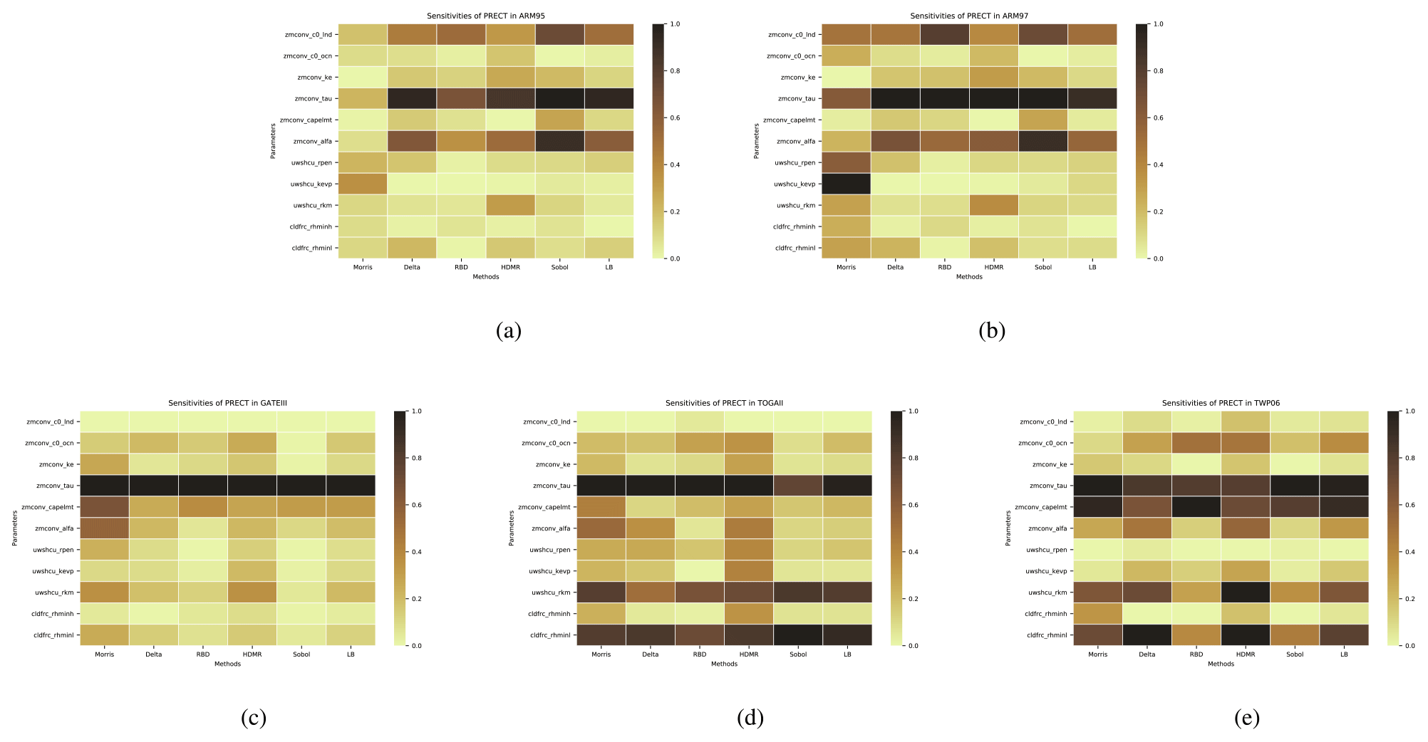
Figure 4 The comparison of the sensitivity of each parameter to PRECT is derived from different analysis methods (including our proposed LB-SCAM) across five cases. Sensitivity results were normalized. (a) ARM95, (b) ARM97, (c) GATEIII, (d) TOGAII, (e) TWP06. The qualitative and quantitative similarities and differences in the sensitivity of each case to each parameter are reflected.

From the results of PRECT, it can be seen that the response of ARM95 and ARM97 to each parameter is basically the same; only a few quantitative differences exist in parameters such as zmconv_alfa, uwshcu_kevp, and so on. Moreover, both cases are sensitive to zmconv_tau, which significantly outweighs the other parameters. For GATEIII, we can see that zmconv_tau similarly has a significant influence on it, but zmconv_alfa and uwshcu_rkm also have a large influence. In addition, the two SA methods of Morris and Sobol simultaneously show that cldfrc_rhminl also has a non-small effect. For TOGAII, it is interesting to find that zmconv_tau and cldfrc_rhminl have similarly significant effects. However, tau still has a far greater influence than other parameters on TWP06, which is similar to ARM95/97. Furthermore, the impact of zmconv_c0_ocn on this case is also notable. This clearly demonstrates that cases located in different locations exhibit varied responses to parameters. To sum up, zmconv_tau has a very significant significance for all cases.

We also compared the differences between these SA methods. To demonstrate the applicability of using our learning-based surrogate model in the SA process, we also show the SA results by using our trained learning-based surrogate models. For comparison across different methods, the most sensitive parameter obtained by each method is tau, but there are differences in the sensitivity of other parameters to some extent. For example, delta and HDMR yield slightly greater sensitivity for the other parameters. In addition, Morris concluded that the sensitivity of these parameters is significantly greater than that of the other methods: that is, the gap between tau and the other parameters is smaller. This may be related to the sampling method, as Morris needs to use a different sequence of samples.

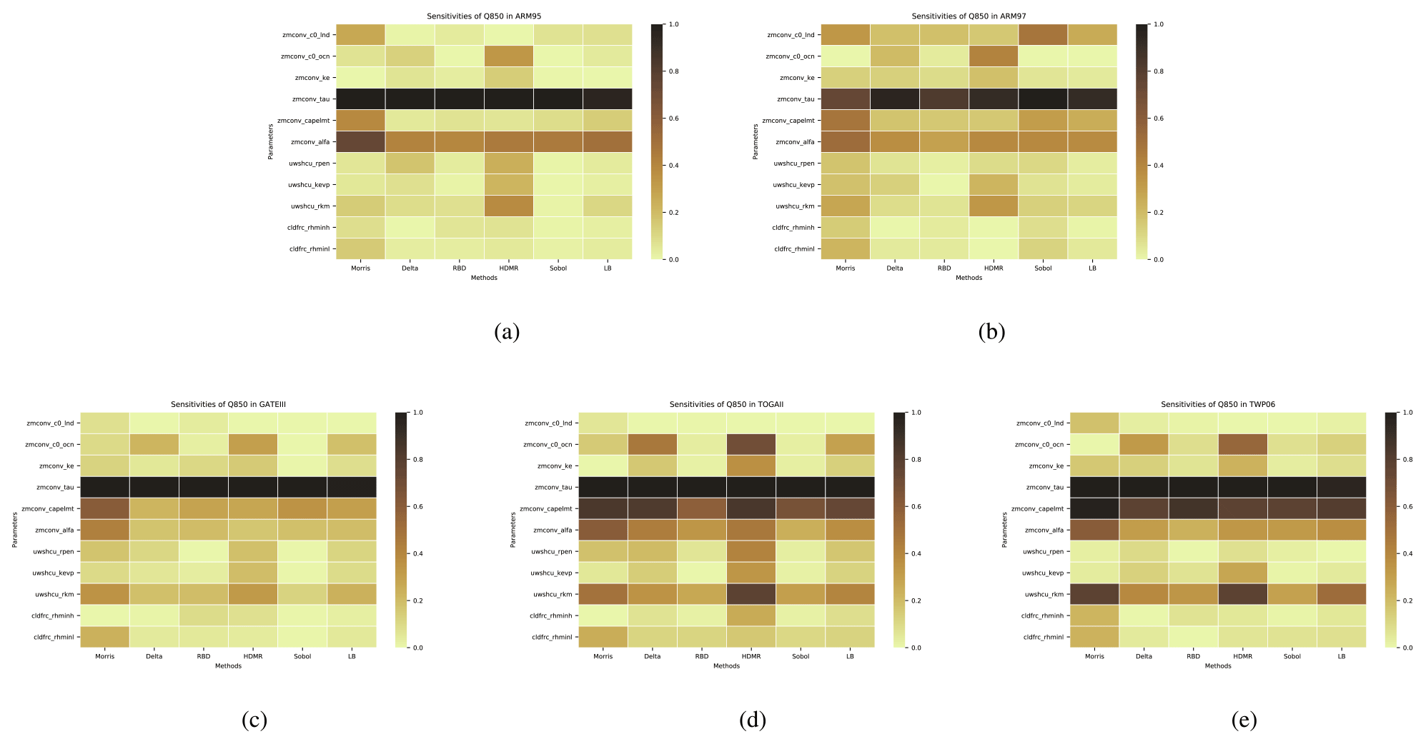
Figure 5 The comparison of the sensitivity of each parameter to Q850 is derived from different analysis methods (including our proposed LB-SCAM) across five cases. Sensitivity results were normalized. (a) ARM95, (b) ARM97, (c) GATEIII, (d) TOGAII, (e) TWP06. The qualitative and quantitative similarities and differences in the sensitivity of each case to each parameter are reflected.

As can be seen from Fig. 5, for the humidity variable Q850, we can clearly see that all five cases are highly sensitive to the parameter zmconv_tau. In addition, the sensitivity of zmconv_alfa is also relatively high. The cases TOGAII and TWP06 exhibit higher sensitivity to zmconv_capelmt, while the other three cases show less pronounced sensitivity. In terms of sensitivity analysis methods, the HDMR method provides more balanced parameter sensitivities, and this is particularly evident in the TOGAII case.

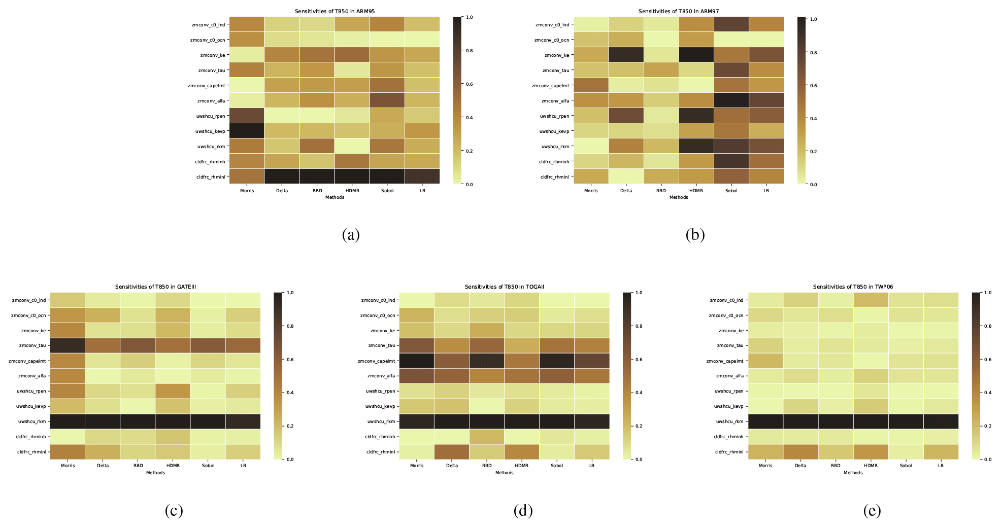
Figure 6 The comparison of the sensitivity of each parameter to T850 is derived from different analysis methods (including our proposed LB-SCAM) across five cases. Sensitivity results were normalized. (a) ARM95, (b) ARM97, (c) GATEIII, (d) TOGAII, (e) TWP06. The qualitative and quantitative similarities and differences in the sensitivity of each case to each parameter are reflected.

As can be seen from Fig. 6, for the temperature variable T850, we can observe some more interesting phenomena. In the ARM95 case, all methods except Morris consider cldfrc_rhminl to be the most significant parameter influencing the results, while Morris concludes that uwshcu_kevp is the strongest, followed by uwshcu_rpen. In the ARM97 case, we find that each SA method identifies different most sensitive parameters, posing a new challenge for our next step in parameter optimization. For the remaining three cases, there is less controversy between different methods. In each case, uwshcu_rkm has overwhelming dominance, and in GATEIII and TOGAII, the impact of zmconv_tau is also considerable. For TOGAII, the sensitivity of zmconv_capelmt and zmconv_alfa should not be overlooked.

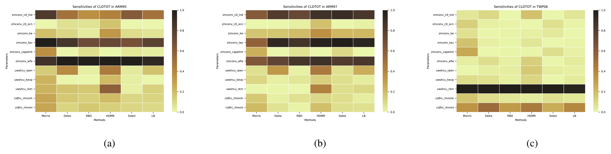
Figure 7 The comparison of the sensitivity of each parameter to CLDTOT comes from different analysis methods (including our proposed LB-SCAM) in three cases. Sensitivity results were normalized. (a) ARM95, (b) ARM97, (c) TWP06. The qualitative and quantitative similarities and differences in the sensitivity of each case to each parameter are reflected.

For the total cloud amount CLDTOT, we can also observe interesting conclusions from Fig. 7. For the ARM95 and ARM97 cases, the results from various methods are consistent: the parameters zmconv_c0_lnd, zmconv_tau, and zmconv_alfa have a significant impact on the results. This reflects the convergence of the two cases. In the case of TWP06, the most noticeable factor is uwshcu_rkm, followed by cldfrc_rhminl. The conclusions drawn by various methods remain consistent.

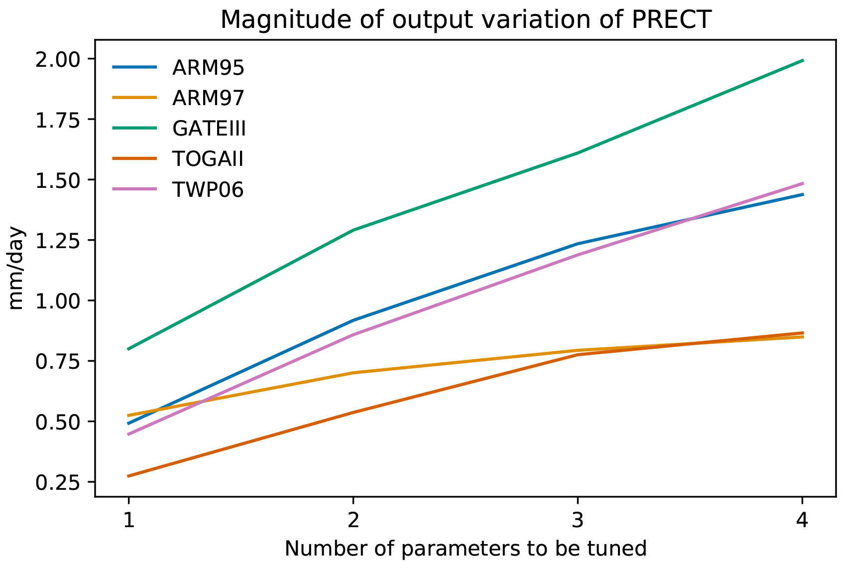
Figure 8 The maximum fluctuation in the output of each case when perturbing one to four parameters. The y axis represents the largest gap between the maximum and minimum values of precipitation output that can occur during the simulation period.

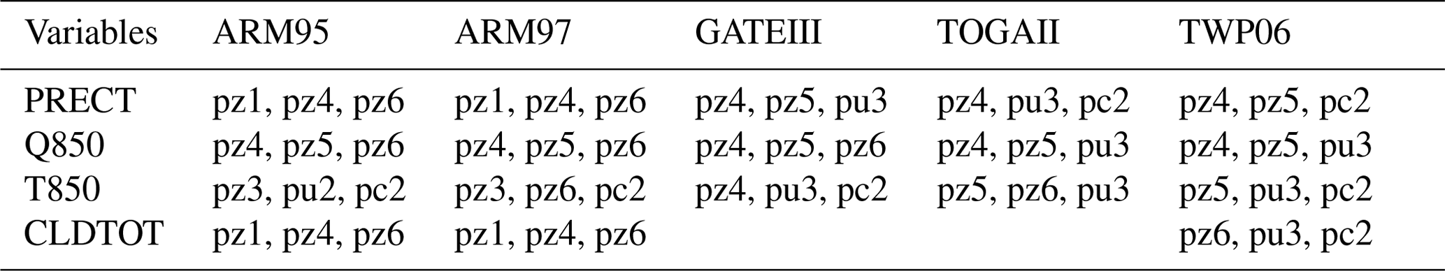
Table 7 The most sensitive parameter combinations of each variable in each case.

4.4 Joint multi-parameter sensitivity analysis using learning-based surrogate models

As mentioned earlier, by using the learning-based surrogate models, we now have the capability to explore the sensitivity of multi-parameter combinations. How many parameters is it reasonable to tune at the same time? Figure 8 illustrates the maximum PRECT output fluctuation that can be brought by different parameter combination sizes. As the number of parameters to be tuned simultaneously increases, the fluctuations that can be brought about are also greater. However, there is also a marginal effect as the number of parameters tuned simultaneously increases. We can see that when tuning four parameters, the gain effect on the result is already not significant. Therefore, considering the range of the most accurate parameter tuning, we limit the number of parameters tuned simultaneously to three. In addition, we also note that for the ARM97 and TOGAII, their precipitation response for four parameters is even smaller than the response of the GATEIII for tuning one parameter. An important reason for this is that these two cases themselves have smaller precipitation values than GATEIII, whereas Fig. 8 uses the absolute values of precipitation.

As our study investigates 11 parameters related to the four variables, there are a total of 165 three-parameter combinations. It would be difficult to test all these combinations using the original SCAM due to the high computational overhead. However, with the help of the surrogate model, we can instead accomplish these tests in less than a minute.

These combinations are listed in Table 7. The whale optimization algorithm (WOA, Mirjalili and Lewis, 2016) has been chosen as the method in this stage. RMSE is also selected as the metric of optimization effect. Next, we will further explore the sensitive parameter combinations.

4.5 Joint optimization for SCAM cases combined with grid search and learning-based models

Consequently, experiments combining the grid search and optimization algorithms will be performed. As above, WOA is still used as the optimization algorithm for this stage. To verify the correctness of the surrogate model, we also compare its output with SCAM.

For the effectiveness of the parameter tuning, the output after tuning is compared with the output of the control experiment (i.e., before tuning) and the observed data after the individual cases had been tuned, as shown in Fig. 9. Here, the experiments with the best optimization results are chosen for comparison. It is easy to see that in the control experiment there are several spikes where the simulated output is significantly higher than the observed values, as is the case in the first four cases. This is to say that these time steps, where the output is significantly larger than the observation in the control trial, are reduced after optimization, making it closer to the observation. This demonstrates the significance of the parameter tuning provided by our proposed LB-SCAM.

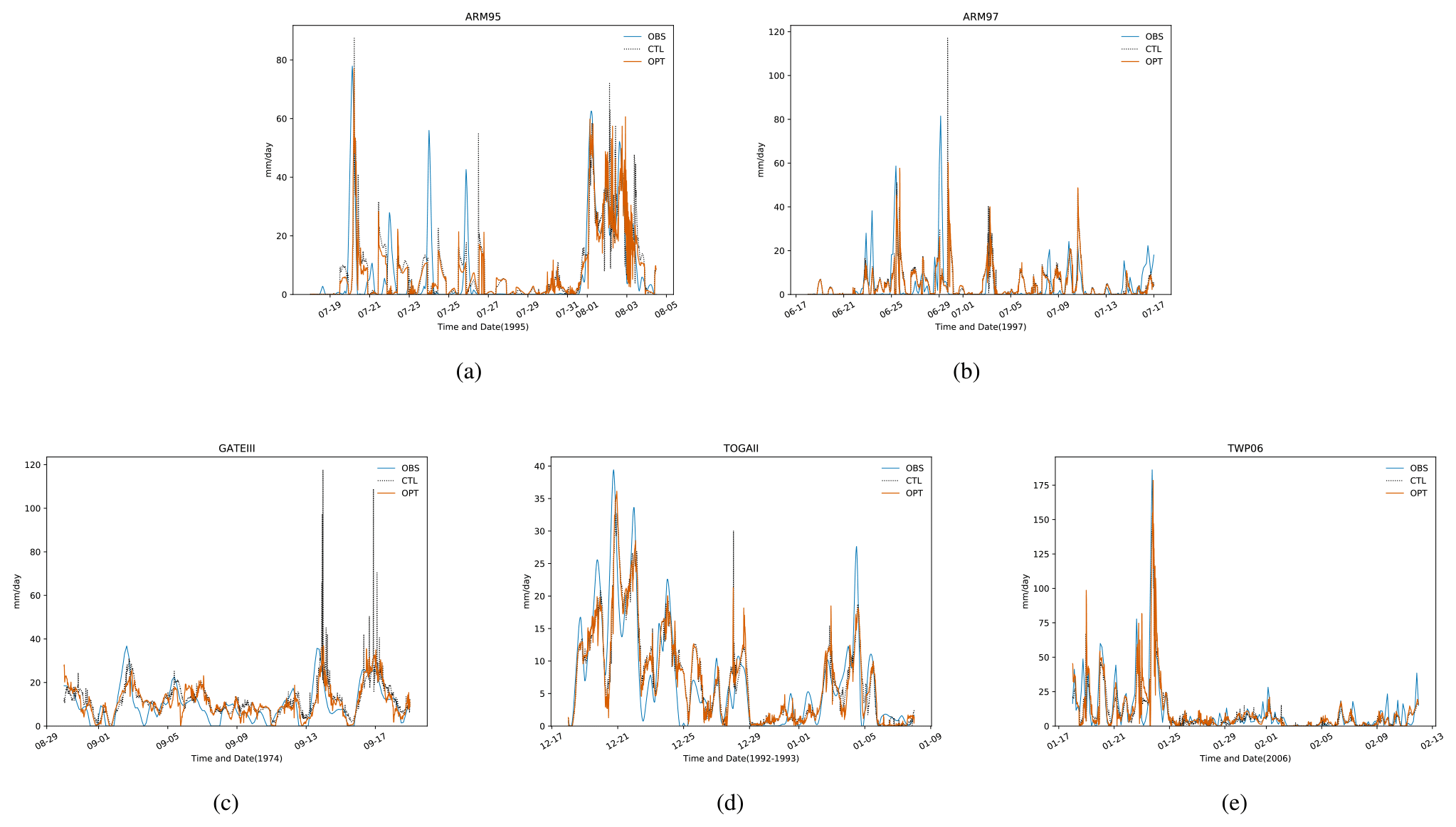
Figure 9 Comparison of SCAM simulation output before and after tuning with observed values in five cases. Here, OBS indicates the observed value, CTL indicates the output before tuning, and OPT indicates the output after tuning. (a) ARM95, (b) ARM97, (c) GATEIII, (d) TOGAII, and (e) TWP06. It can be seen that the optimized output of each case is closer to the observation.

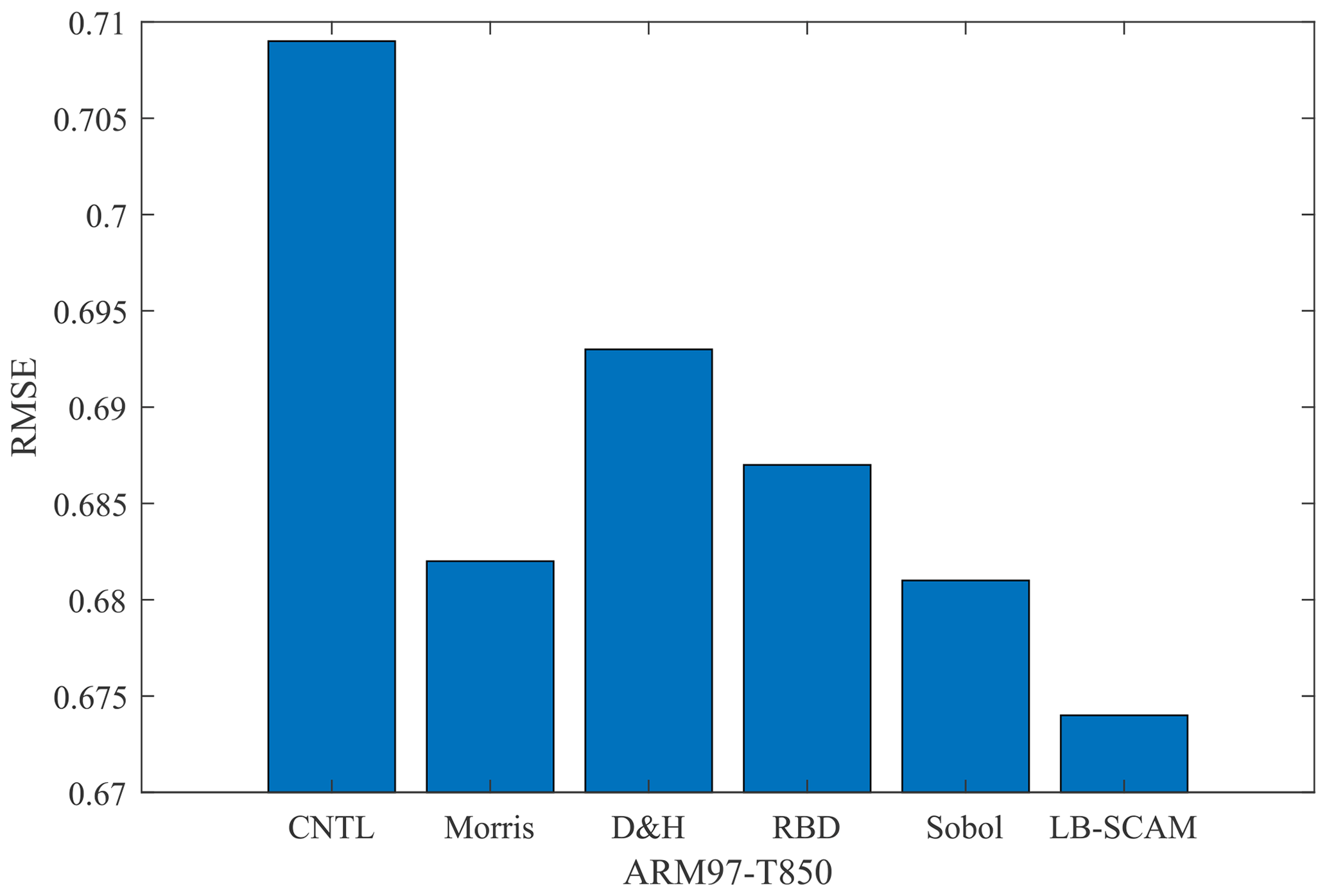
Figure 10 The optimized results of sensitivity parameter combinations for the T850 output variable in the ARM97 case, as provided by various SA methods, are compared with the control experiment. “D&H” represents the common conclusions derived from the delta and HDMR methods.

In contrast to using the optimization algorithm alone, the grid search combined with the optimization algorithm can achieve better results on these SCAM cases. The use of NN trained surrogate models for parameter tuning can further save computational resource overhead and, in terms of results, can meet or exceed traditional optimization methods in most cases.

In the previous sections, we mentioned that different sensitivity analysis methods yielded different conclusions for the output variable T850. Therefore, to demonstrate the performance differences among various methods, we decided to test the optimization results for different parameter combinations, as shown in Fig. 10. Therefore, we can find that it is possible to achieve a win–win situation in terms of computational resources and computational efficiency by training a surrogate model of SCAM based on LB-SCAM.

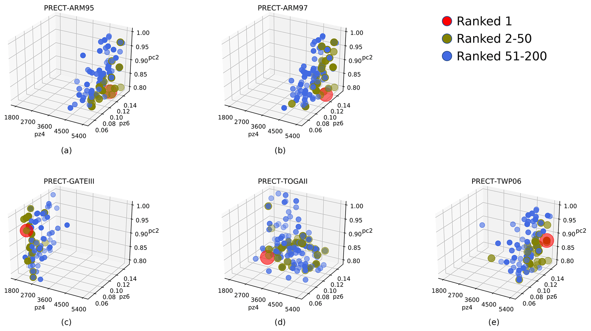
Figure 11 The distribution of parameter solutions performing better for PRECT in each case within the same 3D parameter space. (a) ARM95, (b) ARM97, (c) GATEIII, (d) TOGAII, and (e) TWP06. The points closest to the observed data are shown in red, those ranked 2–50 are shown in olive, and those ranked 51–200 are shown in blue.

After optimization, SCAM cases can get enhancement from 6.4 %–24.4 % in PRECT output, 11.9 %–42.3 % in Q850 output, 5.72 %–22.4 % in T850 output, and 3.8 %–26.1 % in CLDTOT output. Thus, using the proposed method, the main computational overhead comes from sampling and training. The computational overhead can be saved by more than 50 % compared to the case where the above experiments are all run using the full SCAM. In particular, the proposed method demonstrates its effectiveness and usability for situations such as large-scale grid testing, which is almost impossible to accomplish using the full SCAM.

These results also show that the method used in the workflow outperforms previous methods in most cases. Furthermore, the methods in the workflow test a wide range of combinations of values in the parameter space. Thus, using the workflow provides a more complete picture of the parametric characteristics of the different cases in SCAM than optimization algorithms that only provide results but no additional information about the spatial distribution of the parameters. Performing a finer-grained grid search in the vicinity of the optimal value point is also an approach worth testing in the future. From the experimental results, it can be seen that utilizing the surrogate model through sampling with the optimization algorithm not only saves resources but also improves the optimization effect, and meanwhile enhances the robustness of the optimization method.

4.6 A deeper exploration of the relationships between the cases for PRECT

The training of surrogate models makes it possible to conduct larger-scale experiments in a shorter period of time. For the most sensitive combinations of parameters obtained based on the LB method in each case, we can explore the distribution pattern of the results using a grid search. These experiments are carried out on the surrogate model to improve experimental efficiency.

Grid search can also be performed to determine the possible aggregation range of the better-valued solution. To make it easy to compare the same and different cases, we specify the same parameter space for each case. Based on the combined ranking of sensitive parameters under each case, we choose zmconv_tau, zmconv_alfa, and cldfrc_rhminl as the parameter space common to all cases.The results are shown in Fig. 11. The value of each parameter is also divided into 11 levels within its upper and lower bounds. The parameter space remains the same as originally set at the beginning of this paper.

As can be seen, after the parameter space has been replaced, the better-valued solutions for each case show a clear trend towards aggregation, and although the distribution of TOGAII is slightly scattered, it can still be grouped into a cluster. The same parameter space is more conducive to cross-sectional comparisons. It is easy to see that the two land convection cases are closer, which matches our expectations since the two cases are themselves co-located. They have relatively high zmconv_tau and zmconv_alfa and the relatively lowest cldfrc_rhminl. For the three tropical convective cases, their distributions have their own characteristics. TWP06 has the highest tau and alfa, while TOGAII is in the middle for all parameters. The parametric response distributions of GATEIII are much different. Its better performance relies on lower tau and alfa and higher cldfrc_rhminl. As a site that is far away from all other cases, this also coincides with the previous results.

From the results, it can be seen that the distribution of the better values is different for different cases within the same parameter space. A typical example is the parameter zmconv_tau. This reflects the fact that it may be useful and necessary to adopt different parameter configurations for different cases or regions.

Now that we have discovered the pattern that the aggregation range of the more optimal solution for each case by applying a full-space grid search in the same parameter space. From the experimental results, it can be seen that the two cases focusing on land convection are most similar to each other, and two of three cases focusing on tropical convection are also more similar to each other, except for GATEIII.

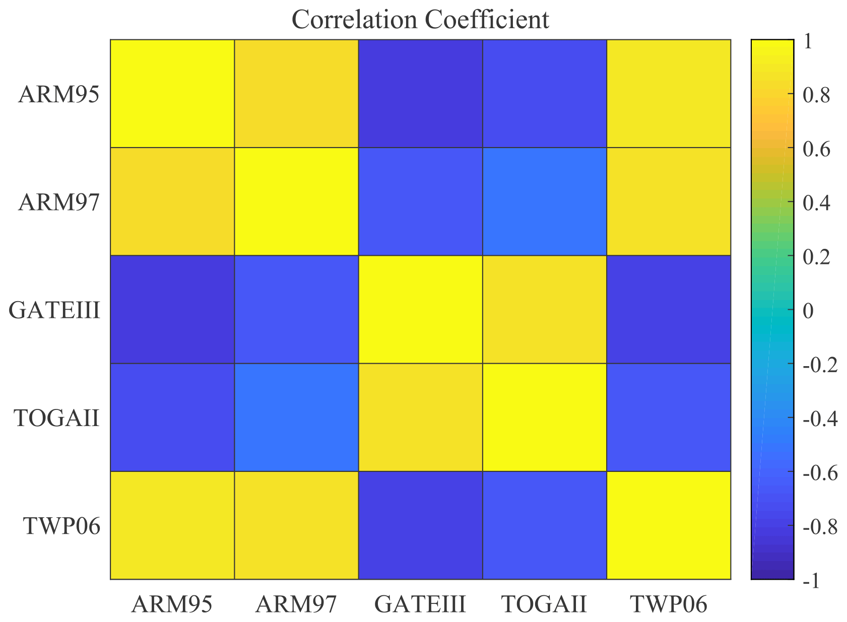
Figure 12 The correlation of the optimal solutions of PRECT for cases within the same parameter space reveals the differences in similarity between different cases.

The Pearson correlation coefficient method is used to compare the best set of values for each case. The obtained similarity is shown in Fig. 12. The average p value in this experiment is less than 0.05, so it is relatively reliable. From this figure, we can see that the parameter values taken between the two cases of land convection are positively correlated in the same parameter space. Two of three cases of tropical convection, TOGAII and TWP06, are also positively correlated with each other. The respective distributions of the above four cases are also positively correlated. The special one is GATEIII, which is negatively correlated with the remaining four cases. These results are also well matched to those obtained in the previous experiments. It is also clear from the results above that SCAM cases in similar locations and of the same type are more relevant when it comes to parameterization.

5 Conclusions

In this paper, we propose a learning-based integrated method for SCAM parameter tuning, enabling a fully automated diagnostic analysis process from sensitive tests to parameter optimization and case comparison. The workflow facilitates large-scale SCAM parameter runs, thereby allowing for more trials in parametric scenario studies within a shorter timeframe. An integrated approach employing several sensitivity methods is utilized for parameter sensitivity analysis. With just one sampling, various SA methods can be invoked for analysis and their results combined.

With the enhancement of artificial intelligence and machine learning techniques, the role played by neural networks in regression analysis has become increasingly evident. In our proposed experimental workflow, multiple regression methods, including NNs incorporating sampling techniques, are likewise used in the parametric analysis process of SCAM. As a precursor to sensitivity analysis, the results of the sampling are used to train an NN-based surrogate model, which validates the accuracy of the sensitivity analysis and improves the parameter tuning process by the surrogate model. In these stages, a grid search strategy for parameter space based on multi-parameter perturbations is used. With the development of computer performance, the method can search for the most suitable parameter values within fewer iterations. The combination of grid search and optimization algorithms can also improve the performance of the optimization algorithm in model parameter tuning. Additionally, the application of neural-network-trained surrogate models can save computational resources, which is beneficial in achieving the goal of green computing.

To verify the completeness and validity of the proposed workflow, multi-group experiments based on five typical SCAM cases are implemented. The sensitivity of the parameters to typical output variables related to precipitation is analyzed. Experiments based on the proposed workflow have shown differences in parameter sensitivities with respect to different cases and output variables. This includes differences between different convection types of cases and differences in the effects of deep and shallow convective precipitation parameterization schemes on respective precipitation. In summary, determining appropriate values for each SCAM case located at different locations is also meaningful for model development. Additionally, this provides a heuristic for future research on similar parameterization schemes in other models.