Terrestrial Ecosystem Model in R (TEMIR) version 1.0: simulating ecophysiological responses of vegetation to atmospheric chemical and meteorological changes

The newly developed offline land ecosystem model Terrestrial Ecosystem Model in R (TEMIR) version 1.0 is described here. This version of the model simulates plant ecophysiological (e.g., photosynthetic and stomatal) responses to varying meteorological conditions and concentrations of CO₂ and ground-level ozone (O₃) based on prescribed meteorological and atmospheric chemical inputs from various sources. Driven by the same meteorological data used in the GEOS-Chem chemical transport model, this allows asynchronously coupled experiments with GEOS-Chem simulations with unique coherency for investigating biosphere–atmosphere chemical interactions. TEMIR agrees well with FLUXNET site-level gross primary productivity (GPP) in terms of both the diurnal and monthly cycles (correlation coefficients R²>0.85 and R²>0.8, respectively) for most plant functional types (PFTs). Grass and shrub PFTs have larger biases due to generic model representations. The model performs best when driven by local site-level meteorology rather than reanalyzed gridded meteorology. Simulation using gridded meteorology agrees well for annual GPP in seasonality and spatial distribution with a global average of 134 Pg C yr⁻¹. Application of Monin–Obukhov similarity theory to infer canopy conditions from gridded meteorology does not improve model performance, predicting an increase of +7 % in global GPP. Present-day O₃ concentrations simulated by GEOS-Chem and an O₃ damage scheme at high sensitivity show a 2 % reduction in global GPP with prominent reductions of up to 15 % in eastern China and the eastern USA. Regional correlations are generally unchanged when O₃ is present and biases are reduced, especially for regions with high O₃ damage. An increase in atmospheric CO₂ concentration of 20 ppmv from the level in 2000 to the level in 2010 modestly decreases O₃ damage due to reduced stomatal uptake, consistent with ecophysiological understanding. Our work showcases the utility of this version of TEMIR for evaluating biogeophysical responses of vegetation to changes in atmospheric composition and meteorological conditions.

1 Introduction

Terrestrial vegetation, as an integral part of the global biosphere, plays many vital roles in regulating the earth system. It facilities a substantial portion of the global land–atmosphere exchange of energy, momentum, and chemical species relevant for climate and atmospheric chemistry. It is a major sink for atmospheric carbon, sequestering an estimated 123 ± 8 Pg C of carbon dioxide (CO₂) from the atmosphere annually through plant photosynthesis (Beer et al., 2010; Le Quéré et al., 2015), albeit with a relatively large observation-constrained range of 119–175 Pg C yr⁻¹.

This vegetation-mediated process of CO₂ sequestration, also known as gross primary productivity (GPP), is a key regulator of climate, and forests in particular are one of the largest providers of climate services (Bonan, 2008). Even before the industrial revolution, human perturbations of natural vegetation for agriculture, timber, and other uses had significant impacts on the natural carbon cycle. About a third of the total cumulative CO₂ emission to date that is due to anthropogenic land cover change could have been emitted before the time of industrialization (Pongratz et al., 2009). Over the 20th century, widespread deforestation was estimated to result in a net warming of 0.13–0.15 °C due to biogeochemical warming (via carbon emission) partly offset by biogeophysical cooling (via higher albedo) (Pongratz et al., 2010). A reversal of historical land use trends, especially in the form of afforestation as well as careful management and preservation of existing forests, has the potential to help mitigate anthropogenic climate change, but the future carbon uptake capacity of forests can be substantially altered by an array of biogeochemical feedback mechanisms as forest ecosystems respond to changing climate and atmospheric composition (Arneth et al., 2010). Various global terrestrial ecosystem models have been employed, either stand-alone or coupled within an earth system model, to estimate future carbon budgets in response to global change. A multi-model comparison estimated that over the 21st century, the terrestrial biosphere can gain 0.2–1.5 Pg C for 1 part per million by volume (ppmv) increase in CO₂ due to fertilization effects but lose 10–90 Pg C per degree increase in global surface temperature as forest ecosystems experience warming and more climatic stress (Arora et al., 2013).

An emerging research interest is the interactions between the terrestrial biosphere and atmospheric chemistry and the roles of short-lived atmospheric species in modulating terrestrial ecosystem functions. On the one hand, terrestrial ecosystems facilitate the removal of air pollutants from the atmosphere via the process of dry deposition, thus providing another important service for human benefits. The consequent health benefits are substantial: 17.4 × 10⁶ t of air pollutants equivalent to USD 6.8 billion of public health cost were removed by forests in the contiguous USA in 2010 alone (Nowak et al., 2014), which is 6 % of the estimated total health cost of USD 109 billion (EUR 145 billion) due to air pollution in the USA in 2010 (Im et al., 2018). Globally it is estimated that dry deposition onto vegetated surfaces accounts for ∼ 20 % of the loss of tropospheric O₃ (Wild, 2007), which is a major air pollutant detrimental to human health. On the other hand, the depositional uptake of O₃ by leaves incurs substantial damage to vegetation, interfering with ecosystem functions and terrestrial biogeochemical cycling. In the process of dry deposition, O₃ diffuses via leaf openings, known as stomata, into the leaf interior, where it impairs plant physiological functions and health. Stomatal uptake itself is responsible for 30 %–90 % of the deposition sink of O₃ (Felzer et al., 2007; Ainsworth et al., 2012). O₃ can significantly disrupt leaf photosynthesis rates, thereby hindering plant growth and reducing forest and crop productivity (Ainsworth et al., 2012). The O₃-induced global yield losses for the key staple crops (wheat, rice, maize, and soybean) for 2000 were estimated to be worth USD 11–26 billion (Van Dingenen et al., 2009; Avnery et al., 2011). For natural vegetation and forests, observed GPP reductions average ∼ 10 % but could regionally be up to 30 % (e.g., Fares et al., 2013; Proietti et al., 2016; Moura et al., 2018). Modeling studies have estimated a 2 %–12 % decrease in GPP due to present-day O₃, with large reductions of more than 20 % in the midlatitude regions of North America, Europe, and East Asia (Anav et al., 2011; Yue and Unger, 2014; Lombardozzi et al., 2015). O₃ damage to plants in turn alters biosphere–atmosphere exchange, with ramifications for both climate and air quality. Models have estimated a 2 %–6 % decrease in global transpiration following O₃ damage. The corresponding reductions in latent heat flux can regionally enhance temperature by up to 2–3 °C and alter rainfall (Li et al., 2016; Sadiq et al., 2017; Zhu et al., 2022).

Accurate predictions of both air quality and ecosystem functions, as well as their interactions, thus require proper representation of ecophysiological processes in the terrestrial ecosystems but are obscured by a complex array of nonlinear interactions between plant physiology, O₃, CO₂, and meteorological drivers. Elevated CO₂ enhances photosynthesis and also induces stomatal closure (reducing stomatal conductance) over various timescales, likely reflecting the adaptation of plants to improve water use efficiency (Noormets et al., 2010; Franks et al., 2013). Sanderson et al. (2007) suggested that a doubling of CO₂ could worsen O₃ air quality by up to +8 ppbv (parts per billion by volume) due to reduced stomatal conductance and dry deposition. O₃ damage to vegetation can potentially lead to a decline in the leaf area index (LAI) and stomatal uptake, which in turn would create strong positive feedback that would further enhance surface O₃ by up to +6 ppbv (Sadiq et al., 2017; Zhou et al., 2018; Zhu et al., 2022). Furthermore, higher humidity generally promotes stomatal opening, while drought conditions often inhibit it (Dermody et al., 2008; Rhea et al., 2010; Monks et al., 2015). A modeling study by Emberson et al. (2013) suggested that the extended drought in association with the 2006 European heatwave might have shut down the dry depositional sink for O₃ as plants closed their stomata to prevent excessive water loss, thereby leading to a greater number of O₃-related premature human deaths. To complicate the matter further, O₃ damage may cause stomata to respond more sluggishly to meteorological conditions. Under certain prolonged conditions (e.g., droughts) such sluggishness of stomatal response may cause them to be more open than without O₃ damage (McLaughlin et al., 2007; Sun et al., 2012; Huntingford et al., 2018). These studies highlight the importance of considering the adaptive responses of plants to changing atmospheric composition and meteorological conditions in predicting future O₃ air quality and ecosystem productivity, yet most atmospheric chemistry models to date rely on semi-empirical formulations for plant-mediated processes (e.g., dry deposition) without resolving ecophysiological processes that may evolve over time. Issues may also arise when coupling atmospheric chemistry and complex ecosystem models due to inconsistent driving inputs and model requirements (Clifton et al., 2020). As interpretation of model results depends largely on the underlying physiological processes, in-depth understanding of system behaviors is crucial yet lacking (Ganzeveld and Lelieveld, 1995; Hardacre et al., 2015).

A number of studies have taken advantage of the Earth System Modeling Framework (ESMF) to dynamically link dry deposition and O₃ fluxes in atmospheric chemistry models to the photosynthetic and stomatal calculations in land surface models (e.g., Ganzeveld et al., 2010; Pacifico et al., 2012; Val Martin et al., 2014; Verbeke et al., 2015; Halladay and Good, 2017; Sadiq et al., 2017; Zhu et al., 2022; Bhattarai et al., 2023). These studies largely focused on long-term averages and trends rather than variability due to climate anomalies. Simulated climate is also often sensitive to land surface changes, and any simulated responses of meteorological variables to plant ecophysiological changes can further modify O₃ through a cascade of feedbacks, potentially obscuring the importance and relative contribution from individual plant-mediated pathways. Fully coupled earth system models contain an intricate network of interdependencies among climate, atmospheric chemistry, and land surface and thus may not be ideal for calibrating specific model processes against observations. Stand-alone or coupled chemical transport models and ecosystem models driven by a consistent set of prescribed “offline” meteorology from observations and reanalysis datasets would be particularly useful to improve the understanding of O₃–vegetation interactions in isolation and enhance model capability in predicting air quality under climate anomalies.

The Terrestrial Ecosystem Model in R version 1.0 (TEMIR v1.0), described in Sect. 2.2, is a stand-alone, multi-parameterization model designed to simulate important canopy and ecophysiological processes that are relevant for ecosystem exchange and atmospheric chemistry, including canopy radiative physics and aerodynamics, photosynthesis, stomatal behaviors, and dry deposition of different chemical species. It is designed to be entirely consistent with the GEOS-Chem global chemical transport model (CTM) in terms of model inputs and land surface representation. Driven by a consistent set of prescribed meteorological and surface flux inputs, asynchronously coupled GEOS-Chem–TEMIR experiments can be performed globally or regionally to simulate plant ecophysiological responses to changing atmospheric composition arising from, for example, O₃ pollution and rising CO₂, as well as to simulate a changing climate as simulated by climate models that have already been coupled to GEOS-Chem. It can also be used with user-defined meteorological and flux inputs (especially those directly from FLUXNET observations; https://fluxnet.fluxdata.org, last access: 21 March 2024) to perform site-level simulations for various purposes, e.g., process investigation, predictions, model validation, and optimization with different parameterization schemes. (Versions of TEMIR with active biogeochemistry and crop biophysics are under development and not within the scope of this paper.) Validation and application of TEMIR to simulate O₃ dry deposition and flux-based metrics of O₃ damage to crops have been presented in several previous studies (i.e., Wong et al., 2019; Tai et al., 2021; Sun et al., 2022).

Developing an ecosystem model in the R programming language is beneficial to various ends. R is an increasingly popular tool for ecological research (R Core Team, 2022), especially in population and community ecology. Lai et al. (2019) surveyed more than 60 000 peer-reviewed ecology journal articles and found that the number of studies reported using R as their primary tool in data analysis increased from ∼ 10 % in 2008 to ∼ 60 % in 2017. However, ecosystem and earth system models are often written in low-level languages, such as Fortran, because the field of ecosystem and earth system modeling has close historical ties with geoscientific research due to the importance of representing the land cover and biogeochemical cycles in climate models, which are most often written in low-level languages that are less accessible to researchers outside of the field. Having a terrestrial ecosystem model in R may help enhance the accessibility to ecosystem modeling for ecological researchers who are more familiar with R, generate a common modeling framework across population, community, and ecosystem scales, and hopefully serve as a bridge between ecological and geoscientific fields to advance interdisciplinarity. Being an entirely free and open software, as well as a highly versatile and relatively user-friendly programming language, it may also help promote open science in environmental research and education, allowing the model to be more widely used as a policy-relevant assessment tool for practitioners such as those who need to assess the carbon uptake potential of tree planting or reforestation as means to achieve carbon neutrality.

2 Model description

2.1 GEOS-Chem model description

GEOS-Chem as a global CTM is widely used in research due to its versatility in tackling a multitude of atmospheric chemistry problems. We use GEOS-Chem v12.2.0 (https://doi.org/10.5281/zenodo.2572887, Bey et al., 2001) driven by assimilated meteorological observations from the Goddard Earth Observing System (GEOS) of the NASA Global Modeling Assimilation Office (GMAO). The driving meteorological data are available in 1-hourly and 3-hourly temporal resolutions with the finest horizontal resolution of 0.25° latitude by 0.3125° longitude and 72 hybrid vertical levels extending from the surface to 0.01 hPa, provided by the GEOS-Forward Processing product (GEOS-FP). Coarser resolutions of the reanalysis product Modern-Era Retrospective Analysis for Research and Applications v2 (MERRA-2) (Gelaro et al., 2017), which is a historical dataset spanning from 1980 to the present, can also be used. GEOS-Chem is equipped with detailed O₃–NO_x–VOC–aerosol chemical mechanisms (NO_x: nitrogen oxides; VOC: volatile organic compound) that are used for simulating atmospheric chemistry and have been validated by many studies (e.g., Bey et al., 2001; Parrington et al., 2008; Zhang et al., 2010; Zhang and Wang, 2016; Hu et al., 2018). Anthropogenic missions of many species (e.g., CO, NO_x, and non-methane VOCs) can be taken from global inventories (e.g., Community Emissions Data System – CEDS; Hoesly et al., 2018) and/or regional inventories through the Harmonized Emissions Component (HEMCO) v2.1 (Keller et al., 2014; Lin et al., 2021). Biogenic emissions are calculated online with the Model of Emissions of Gases and Aerosols from Nature (MEGAN) v2.1 (Guenther et al., 2012). An alternative photosynthesis-based isoprene emission (Pacifico et al., 2011) is also available (Lam et al., 2023). In this study, the meteorological input used for global simulations of both GEOS-Chem and TEMIR is the MERRA-2 product at a resolution of 2° × 2.5° latitude by longitude. The surface O₃ concentrations simulated by GEOS-Chem are used as inputs for TEMIR to simulate the corresponding vegetation responses under the consistent set of MERRA-2 meteorology.

2.2 TEMIR description

TEMIR computes biogeophysical responses of terrestrial ecosystems to changes in the atmospheric (e.g., [CO₂]) and terrestrial environment. Driven by the same consistent meteorological and land surface input data as GEOS-Chem, TEMIR is designed to be highly compatible with GEOS-Chem and can be coupled asynchronously with simulated atmospheric composition (e.g., [O₃]) from GEOS-Chem, which is a vital aspect for the objectives of this study.

2.2.1 Plant type representation

Plant type categories considered in TEMIR follow the convention of the Community Land Model v4.5 (CLM4.5) (Oleson et al., 2013), embedded within the Community Earth System Model (CESM) v1.2.2. The plant type categories consist of 14 natural vegetation types (including generic C₃ crops) (Lawrence and Chase, 2007) and 10 rainfed or irrigated crop types (Table S1 in the Supplement), giving a total of 24 different plant function types (PFTs), as well as one land type for unvegetated land or bare ground. Each model grid cell consists of a mosaic of natural or managed PFTs and/or bare ground, where only the natural PFTs share a single soil column, allowing them theoretically to compete for soil water. Each PFT or bare ground has a prescribed present-day fractional coverage in each grid cell, derived from Moderate Resolution Imaging Spectroradiometer (MODIS) satellite data (Lawrence and Chase, 2007) according to climatic (temperature- and precipitation-based) rules (see Table 3 of Bonan et al., 2002), as well as managed crop distribution for non-generic crops (corn, temperate and winter cereals, and soybean) (Portmann et al., 2010). Each PFT has its own characteristic structural and physiological parameters (Table S2) as detailed in Oleson et al. (2013). The parameters used to represent vegetation structure include LAI, stem area index (SAI), and canopy height (h). This version of TEMIR lacks a full carbon cycle, and thus these structural parameters are prescribed as model input data. The monthly PFT-level LAI is derived from MODIS using the deaggregation methods described in Lawrence and Chase (2007), and the PFT-level SAI is derived from the LAI using the methods of Zeng et al. (2002). The PFT-level canopy heights are prescribed following Bonan et al. (2002). Users can specify any gridded total LAI input data, whereby the PFT-specific LAI that TEMIR requires is then scaled accordingly. This version of TEMIR does not dynamically simulate PFT coverage and structural parameters, and thus competition among different plant strategies or adaptation to environmental changes, such as climate change and air pollution, is not simulated. The effects of land use and land cover change (LULCC) or changing plant type distribution due to adaptation can only be included by user-modified prescribed PFT fractional coverage or LAI data obtained externally from other models or studies. These input data can, however, be updated every simulation year to represent continuous LULCC over interannual to multi-decadal timescales. Model development for a full carbon cycle for both natural vegetation and crops (Tai et al., 2021) is actively ongoing.

2.2.2 Canopy radiative transfer

Each PFT simulated per vegetated grid cell is represented as a single “big-leaf” canopy of sunlit and shaded leaves. We implement two alternative canopy radiative transfer schemes to calculate the sunlit and shaded LAI (LAI_sun and LAI_sha), absorbed photosynthetically active radiation (PAR) by sunlit and shaded leaves (ϕ_sun and ϕ_sha, in W m⁻²), canopy light extinction coefficient (K_b), surface albedo and other radiative variables as functions of direct beam and diffuse incident PAR reaching the canopy top (I_dir and I_diff, in W m⁻²), cosine of the solar zenith angle (μ), and other vegetation parameters. The default scheme follows the two-stream approximation of Dickinson (1983) and Sellers (1985), which considers light attenuation by both leaves and stems. The details of the scheme are described in Sects. 3.1, 3.3, and 4.1 of Oleson et al. (2013). In brief, the absorbed PAR averaged over the sunlit and shaded canopy per unit plant area (leaf plus stem area) is

$$\begin{array}{}\text{(1)}& {\displaystyle }{\mathit{\varphi }}_{\mathrm{sun}}={\displaystyle \frac{f_{\mathrm{sun},\mathrm{dir}}{I}_{\mathrm{dir}}+f_{\mathrm{sun},\mathrm{diff}}{I}_{\mathrm{diff}}}{{\mathrm{PAI}}_{\mathrm{sun}}}},\text{(2)}& {\displaystyle }{\mathit{\varphi }}_{\mathrm{sha}}={\displaystyle \frac{f_{\mathrm{sha},\mathrm{dir}}{I}_{\mathrm{dir}}+f_{\mathrm{sha},\mathrm{diff}}{I}_{\mathrm{diff}}}{{\mathrm{PAI}}_{\mathrm{sha}}}},\end{array}$$

where $f_{\mathrm{sun}/\mathrm{sha},\mathrm{dir}/\mathrm{diff}}$ is the fraction of direct or diffuse incident radiation absorbed by the sunlit or shaded leaves and stems as calculated by the two-stream approach. The sunlit and shaded plant area index (PAI = LAI + SAI) is

$$\begin{array}{}\text{(3)}& {\displaystyle }{\mathrm{PAI}}_{\mathrm{sun}}={\displaystyle \frac{\mathrm{1}-e^{-K_b\left(\mathrm{LAI}+\mathrm{SAI}\right)}}{K_b}},\text{(4)}& {\displaystyle }{\mathrm{PAI}}_{\mathrm{sha}}=\left(\mathrm{LAI}+\mathrm{SAI}\right)-{\mathrm{PAI}}_{\mathrm{sun}},\end{array}$$

and K_b is calculated following the two-stream approximation. The sunlit and shaded LAIs ultimately used to calculate canopy photosynthesis are

$$\begin{array}{}\text{(5)}& {\displaystyle }{\mathrm{LAI}}_{\mathrm{sun}}={\mathrm{PAI}}_{\mathrm{sun}}{\displaystyle \frac{\mathrm{LAI}}{\mathrm{LAI}+\mathrm{SAI}}},\text{(6)}& {\displaystyle }{\mathrm{LAI}}_{\mathrm{sha}}={\mathrm{PAI}}_{\mathrm{sha}}{\displaystyle \frac{\mathrm{LAI}}{\mathrm{LAI}+\mathrm{SAI}}}.\end{array}$$

An alternative simplified scheme that accounts for light attenuation by leaves only following the convention of the Zhang et al. (2002) dry deposition model as modified from Norman (1982), which is also implemented in TEMIR (see Sect. 2.2.6), is implemented as follows.

$$\begin{array}{}\text{(7)}& {\displaystyle }\begin{array}{rl}{\mathit{\varphi }}_{\mathrm{sha}}& =I_{\mathrm{diff}}\exp \left(-\mathrm{0.5}{\mathrm{LAI}}^a\right)\\ & +\mathrm{0.07}{I}_{\mathrm{dir}}\left(\mathrm{1.1}-\mathrm{0.1}\mathrm{LAI}\right)\exp \left(-\mathit{\mu }\right)\end{array}\text{(8)}& {\displaystyle }{\mathit{\varphi }}_{\mathrm{sun}}={\mathit{\varphi }}_{\mathrm{sha}}+K_b{I}_{\mathrm{dir}}^b\text{(9)}& {\displaystyle }{K}_b={\displaystyle \frac{\mathrm{0.5}}{\mathit{\mu }}}\text{(10)}& {\displaystyle }{\mathrm{LAI}}_{\mathrm{sun}}={\displaystyle \frac{\mathrm{1}-e^{-K_b\mathrm{LAI}}}{K_b}}\text{(11)}& {\displaystyle }{\mathrm{LAI}}_{\mathrm{sha}}=\mathrm{LAI}-{\mathrm{LAI}}_{\mathrm{sun}}\end{array}$$

Here, exponent a=0.7 and exponent b=1 for LAI < 2.5 or downwelling shortwave radiation flux $S\downarrow <\mathrm{200}$ W m⁻²; otherwise, a=0.8 and b=0.8.

2.2.3 Canopy photosynthesis and conductance

Leaf photosynthesis of both C₃ and C₄ plants is represented by the well-established formulation that relates to Michaelis–Menten enzyme kinetics and photosynthetic biochemical pathways (Farquhar et al., 1980; von Caemmerer and Farquhar, 1981; Collatz et al., 1991, 1992), a formulation which considers three limiting regimes as given below.

• i.

  The Rubisco-limited photosynthesis rate (A_c, in µmol CO₂ m⁻² s⁻¹) captures the rate of carbon assimilation when substrate availability or enzyme activity is the limiting factor:

  $$\begin{array}{}\text{(12)}& A_{\mathrm{c}}=\left\{\begin{array}{cc}{V}_{\mathrm{cmax}}\frac{c_{\mathrm{i}}-{\mathrm{\Gamma }}_{\ast }}{c_{\mathrm{i}}+K_{\mathrm{c}}\cdot \left(\mathrm{1}+\frac{o_{\mathrm{i}}}{K_{\mathrm{o}}}\right)}& {\text{for C}}_{\mathrm{3}}\text{plants}\\ V_{\mathrm{cmax}}& {\text{for C}}_{\mathrm{4}}\text{plants},\end{array}\right.\end{array}$$

  where c_i (in Pa) is the intercellular CO₂ partial pressure; K_c and K_o are the Michaelis–Menten constants for carboxylation and oxygenation (in Pa), respectively; o_i (in Pa) is the intercellular oxygen partial pressure; Γ_∗ (in Pa) is the CO₂ compensation point; and V_cmax (in µmol CO₂ m⁻² s⁻¹) is the maximum rate of carboxylation.

• ii.

  The RuBP-limited photosynthetic rate (A_j, in µmol CO₂ m⁻² s⁻¹) defines the photosynthesis rate, as light intensity and thus RuBP regeneration are the limiting factors:

  $$\begin{array}{}\text{(13)}& A_j=\left\{\begin{array}{cc}\frac{J}{\mathrm{4}}\left(\frac{c_{\mathrm{i}}{\mathrm{\Gamma }}_{\ast }}{c_{\mathrm{i}}+\mathrm{2}{\mathrm{\Gamma }}_{\ast }}\right)& {\text{for C}}_{\mathrm{3}}\text{plants}\\ \mathrm{0.23}\mathit{\varphi }& {\text{for C}}_{\mathrm{4}}\text{plants},\end{array}\right.\end{array}$$

  where J (in µmol m⁻² s⁻¹) is the electron transport rate and ϕ (in W m⁻²) is the absorbed PAR for either sunlit (ϕ_sun) or shaded (ϕ_sha) leaves as calculated by the canopy radiative transfer model (Sect. 2.2.2). For C₃ plants, J is determined by ϕ as well and is determined as the smaller of the two roots of the following quadratic equation:

  $$\begin{array}{}\text{(14)}& {\mathrm{\Theta }}_{\mathrm{PSII}}{J}^{\mathrm{2}}-\left(I_{\mathrm{PSII}}+J_{\max }\right)J+I_{\mathrm{PSII}}{J}_{\max }=\mathrm{0},\end{array}$$

  where J_max (in µmol m⁻² s⁻¹) is the maximum potential rate of electron transport, Θ_PSII=0.7 is the curvature parameter, and I_PSII (in µmol m⁻² s⁻¹) is the light utilized in electron transport by photosystem II, determined by

  $$\begin{array}{}\text{(15)}& I_{\mathrm{PSII}}=\mathrm{2.3}{\mathrm{\Phi }}_{\mathrm{PSII}}\mathit{\varphi },\end{array}$$

  where Φ_PSII=0.85 is the quantum yield of photosystem II.

• iii.

  The product-limited photosynthetic rate (A_p, in µmol CO₂ m⁻² s⁻¹) represents the limitation from the regeneration rate of photosynthetic phosphate compounds:

  $$\begin{array}{}\text{(16)}& A_{\mathrm{p}}=\left\{\begin{array}{cc}\mathrm{3}{T}_{\mathrm{p}}& {\text{for C}}_{\mathrm{3}}\text{plants}\\ k_{\mathrm{p}}\frac{c_{\mathrm{i}}}{P_{\mathrm{atm}}}& {\text{for C}}_{\mathrm{4}}\text{plants},\end{array}\right.\end{array}$$

  where T_p is the triose phosphate utilization rate (in µmol m⁻² s⁻¹), P_atm (in Pa) is the ambient atmospheric pressure, and k_p is the initial slope of the CO₂ response curve for C₄ plants.

The model considers co-limitation (Collatz et al., 1991, 1992), and the leaf-level gross photosynthesis rate (A, in µmol CO₂ m⁻² s⁻¹) is given by the smaller root of the following equations:

$$\begin{array}{}\text{(17)}& \begin{array}{rl}& {\mathrm{\Theta }}_{\mathrm{c}j}{A}_i^{\mathrm{2}}-\left(A_{\mathrm{c}}+A_j\right)A_i+A_{\mathrm{c}}{A}_j=\mathrm{0},\\ & {\mathrm{\Theta }}_{\mathrm{ip}}{A}^{\mathrm{2}}-\left(A_i+A_{\mathrm{p}}\right)A+A_i{A}_{\mathrm{p}}=\mathrm{0}.\end{array}\end{array}$$

where Θ_cj=0.98 for C₃ plants and Θ_cj=0.80 for C₄ plants, and Θ_ip=0.95 for both. The net photosynthesis rate (A_n, in µmol CO₂ m⁻² s⁻¹) is then

$$\begin{array}{}\text{(18)}& \begin{array}{rl}& A_{\mathrm{n}}=A-R_{\mathrm{d}}\\ & R_{\mathrm{d}}=\\ & \left\{\begin{array}{l}\mathrm{0.015}{V}_{\mathrm{cmax}}\frac{f_{R_{\mathrm{d}}}\left(T_v\right)}{f_{V_{\mathrm{cmax}}}\left(T_v\right)}\\ {\text{for C}}_{\mathrm{3}}\text{plants}\\ \mathrm{0.025}{V}_{\mathrm{cmax}}\left(\frac{\left(\mathrm{1}+\exp \left[s_{\mathrm{1}}\left(T_v-s_{\mathrm{2}}\right)\right]\right)\left(\mathrm{1}+\exp \left[s_{\mathrm{3}}\left(T_v-s_{\mathrm{4}}\right)\right]\right)}{\mathrm{1}+\exp \left[s_{\mathrm{5}}\left(T_v-s_{\mathrm{6}}\right)\right]}\right)\\ \mathrm{for}{\mathrm{C}}_{\mathrm{4}}\text{plants},\end{array}\right.\end{array}\end{array}$$

where R_d (in µmol CO₂ m⁻² s⁻¹) is the dark respiration rate; s₁, s₃, and s₅ are 0.3, 0.2, and 1.3 K, respectively; s₂, s₄, and s₆ are 313.15, 288.15, and 328.15 K⁻¹, respectively; T_v is leaf temperature (in degrees K); and $f_{R_{\mathrm{d}}}\left(T_v\right)$ and $f_{V_{\mathrm{cmax}}}\left(T_v\right)$ are functions to adjust for variations due to temperature (Bonan et al., 2011). All of the parameters (V_cmax, J_max, T_p, R_d, K_c, K_o, Γ_∗, and k_p) are temperature-dependent and scale with their respective PFT-specific standard values at 25 °C by different formulations. Temperature acclimation of V_cmax and J_max from the previous 10 d, as well as day-length dependence of V_cmax, is implemented as the default option. These are all detailed in Sects. 8.2 and 8.3 of Oleson et al. (2013).

The calculation of photosynthesis rates described above is coupled with that of stomatal conductance of water (g_s, in m s⁻¹) following the formulation of Ball et al. (1987) with m and b being the slope and intercept parameters derived from empirical data:

$$\begin{array}{}\text{(19)}& g_{\mathrm{s}}=\mathit{\alpha }\left(m{A}_{\mathrm{n}}{\displaystyle \frac{\frac{{\mathrm{e}}_{\mathrm{s}}}{e_{\mathrm{sat}}}}{\frac{c_{\mathrm{s}}}{P_{\mathrm{atm}}}}}+b\right),\end{array}$$

where g_s is controlled by the leaf surface CO₂ partial pressure c_s (in Pa), leaf surface water vapor pressure e_s (in Pa), and temperature-dependent saturation vapor pressure e_sat (in Pa); m=9 and b=10 000 µmol m⁻² s⁻¹ for C₃ plants, and m=4 and b=40 000 µmol m⁻² s⁻¹ for C₃ plants; and the factor α converts the unit of conductances from µmol H₂O m⁻² s⁻¹, which is more common in ecophysiology literature, to m s⁻¹, which is common in atmospheric science literature:

$$\begin{array}{}\text{(20)}& \mathit{\alpha }={\displaystyle \frac{{\mathrm{10}}^{-\mathrm{6}}{R}_{\mathrm{uni}}{\mathit{\theta }}_{\mathrm{atm}}}{P_{\mathrm{atm}}}},\end{array}$$

where R_uni=8.314468 J K⁻¹ mol⁻¹ is the universal gas constant and θ_atm (in degrees K) is the ambient atmospheric potential temperature. An alternative stomatal conductance scheme (Medlyn et al., 2011; Franks et al., 2017) is also implemented:

$$\begin{array}{}\text{(21)}& g_{\mathrm{s}}=\mathit{\alpha }\left[\mathrm{1.6}\left(\mathrm{1}+{\displaystyle \frac{m}{\sqrt{\mathrm{VPD}}}}\right){\displaystyle \frac{A_{\mathrm{n}}}{\frac{c_{\mathrm{s}}}{P_{\mathrm{atm}}}}}+b\right],\end{array}$$

where VPD = 0.001(e_sat−e_s) (in kPa) is the vapor pressure deficit, m has PFT-specific values consistent with CLM5.0 (Sect. 9.3 of Lawrence et al., 2020), and b=100 µmol m⁻² s⁻¹. Photosynthesis and stomatal conductance are further related by the diffusive flux equations for CO₂ and water vapor:

$$\begin{array}{}\text{(22)}& {\displaystyle }\begin{array}{rl}{A}_{\mathrm{n}}& ={\displaystyle \frac{\mathrm{1}}{\mathit{\alpha }}}{\left({\displaystyle \frac{\mathrm{1.4}}{g_{\mathrm{b}}}}+{\displaystyle \frac{\mathrm{1.6}}{g_{\mathrm{s}}}}\right)}^{-\mathrm{1}}{\displaystyle \frac{c_{\mathrm{a}}-c_{\mathrm{i}}}{P_{\mathrm{atm}}}}={\displaystyle \frac{g_{\mathrm{b}}}{\mathrm{1.4}\mathit{\alpha }}}{\displaystyle \frac{c_{\mathrm{a}}-c_{\mathrm{s}}}{P_{\mathrm{atm}}}}\\ & ={\displaystyle \frac{g_{\mathrm{s}}}{\mathrm{1.6}\mathit{\alpha }}}{\displaystyle \frac{c_{\mathrm{s}}-c_{\mathrm{i}}}{P_{\mathrm{atm}}}},\end{array}\text{(23)}& {\displaystyle }\begin{array}{rl}{E}^{\prime }& ={\displaystyle \frac{\mathrm{1}}{\mathit{\alpha }}}{\left({\displaystyle \frac{\mathrm{1}}{g_{\mathrm{b}}}}+{\displaystyle \frac{\mathrm{1}}{g_{\mathrm{s}}}}\right)}^{-\mathrm{1}}{\displaystyle \frac{e_{\mathrm{a}}-e_i}{P_{\mathrm{atm}}}}={\displaystyle \frac{g_{\mathrm{b}}}{\mathit{\alpha }}}{\displaystyle \frac{e_{\mathrm{a}}-e_{\mathrm{s}}}{P_{\mathrm{atm}}}}\\ & ={\displaystyle \frac{g_{\mathrm{s}}}{\mathit{\alpha }}}{\displaystyle \frac{e_{\mathrm{s}}-e_i}{P_{\mathrm{atm}}}},\end{array}\end{array}$$

where c_a (in Pa) and e_a (in Pa) are the canopy air CO₂ partial and water vapor pressure, e_i (in Pa) is the saturation vapor pressure at the leaf temperature, E^′ (in µmol H₂O m⁻² s⁻¹) is the transpiration flux, and g_b (in m s⁻¹) is the leaf boundary layer conductance:

$$\begin{array}{}\text{(24)}& g_{\mathrm{b}}=C_{\mathrm{v}}\sqrt{{\displaystyle \frac{u_{\ast }}{d_{\mathrm{l}}}}}.\end{array}$$

The photosynthesis–stomatal conductance model considers limitation arising from soil water stress. A soil water stress factor (β_t) scales the photosynthesis rate and stomatal conductance, being multiplied directly to A, R_d in Eq. (18) and b in Eq. (19) or Eq. (21) to account for soil water stress (Porporato et al., 2001; Verhoef and Egea, 2014). To compute β_t, we consider a two-layer soil model consisting of a topsoil layer (0–5 cm) and a root zone beneath the top soil (5–100 cm), consistent with and constrained by the input soil moisture and model structure of MERRA-2. First, the soil matric potential in each layer i, ψ_i (in mm), that represents water availability in ecophysiological terms is evaluated as a function of soil wetness (s_i) and soil type:

$$\begin{array}{}\text{(25)}& {\mathit{\psi }}_i={\mathit{\psi }}_{\mathrm{sat},i}{s}_i^{-B_i},\end{array}$$

where ψ_sat,i and B_i refer to the saturated soil matric potential and soil water characteristic parameter, respectively, both depending on soil texture. A wilting factor, w_i, is formulated as a function of ψ_i as well as ψ_c and ψ_o (Table S2), which refer to the matric potential at which stomatal closure and stomatal opening occur to the full extent, respectively:

$$\begin{array}{}\text{(26)}& w_i=\left\{\begin{array}{l}\mathrm{1}\mathrm{for}{\mathit{\psi }}_i>{\mathit{\psi }}_{\mathrm{o}}\\ \frac{{\mathit{\psi }}_{\mathrm{c}}-{\mathit{\psi }}_i}{{\mathit{\psi }}_{\mathrm{c}}-{\mathit{\psi }}_{\mathrm{o}}}\mathrm{for}{\mathit{\psi }}_{\mathrm{c}}\le {\mathit{\psi }}_i\le {\mathit{\psi }}_{\mathrm{o}}\\ \mathrm{0}\mathrm{for}{\mathit{\psi }}_i<{\mathit{\psi }}_{\mathrm{c}}.\end{array}\right.\end{array}$$

The function β_t is then the average of the wilting factors weighted by the PFT-specific root fraction (r_i) in each layer:

$$\begin{array}{}\text{(27)}& {\mathit{\beta }}_t=\sum _{i=\mathrm{1}}^{\mathrm{2}}{w}_i{r}_i.\end{array}$$

A single-layer bulk soil formulation considering only the root zone (0–100 cm) is also implemented but is found to be inferior to the two-layer formulation in terms of reproducing observed GPP in semiarid locations (Lam and Tai, 2020).

The above equations calculate photosynthesis and conductance at the leaf level only, and appropriate scaling to account for vertical variation in leaf nitrogen content, light attenuation, and sunlit vs. shaded leaves is needed to obtain the canopy-level photosynthesis (i.e., GPP) and conductance. This is done by scaling V_cmax and other parameters as follows:

$$\begin{array}{}\text{(28)}& {\displaystyle }{V}_{\mathrm{cmax},\mathrm{sun}}=V_{\mathrm{cmax},\mathrm{top}}{\displaystyle \frac{\mathrm{1}-e^{-\left(K_{\mathrm{n}}+K_b\right)\mathrm{LAI}}}{K_{\mathrm{n}}+K_b}}{\displaystyle \frac{\mathrm{1}}{{\mathrm{LAI}}_{\mathrm{sun}}}},\text{(29)}& {\displaystyle }\begin{array}{rl}& V_{\mathrm{cmax},\mathrm{sha}}=\\ & V_{\mathrm{cmax},\mathrm{top}}\left[{\displaystyle \frac{\mathrm{1}-e^{-K_{\mathrm{n}}\mathrm{LAI}}}{K_{\mathrm{n}}}}-{\displaystyle \frac{\mathrm{1}-e^{-\left(K_{\mathrm{n}}+K_b\right)\mathrm{LAI}}}{K_{\mathrm{n}}+K_b}}\right]{\displaystyle \frac{\mathrm{1}}{{\mathrm{LAI}}_{\mathrm{sha}}}},\end{array}\end{array}$$

where V_cmax, sun and V_cmax, sha are the canopy-averaged leaf-level values for V_cmax for sunlit and shaded leaves, respectively, which are used to compute leaf-level photosynthesis and stomatal conductance for sunlit and shaded leaves separately (A_sun, A_sha, g_ssun, and g_ssha) from the equations above. K_n=0.30 is the canopy decay coefficient for nitrogen, calculated and calibrated to match an explicit multi-layer canopy (Bonan et al., 2012; Oleson et al., 2013). V_cmax, top is the PFT-specific value for V_cmax for the top of the canopy. K_b, LAI_sun, and LAI_sha are computed from the canopy radiative transfer model (Sect. 2.2.2). Other parameters, i.e., J_max, T_p, k_p, and R_d, scale similarly.

Canopy photosynthesis rate (i.e., GPP, in µmol CO₂ m⁻² s⁻¹) and canopy conductance (g_can, in m s⁻¹) per unit land area of a given PFT are then

$$\begin{array}{}\text{(30)}& {\displaystyle }\mathrm{GPP}=A_{\mathrm{sun}}{\mathrm{LAI}}_{\mathrm{sun}}+A_{\mathrm{sha}}{\mathrm{LAI}}_{\mathrm{sha}},\text{(31)}& {\displaystyle }\begin{array}{rl}{g}_{\mathrm{can}}& ={\left({\displaystyle \frac{\mathrm{1}}{g_{\mathrm{b}}}}+{\displaystyle \frac{\mathrm{1}}{g_{\mathrm{ssun}}}}\right)}^{-\mathrm{1}}{\mathrm{LAI}}_{\mathrm{sun}}\\ & +{\left({\displaystyle \frac{\mathrm{1}}{g_{\mathrm{b}}}}+{\displaystyle \frac{\mathrm{1}}{g_{\mathrm{ssha}}}}\right)}^{-\mathrm{1}}{\mathrm{LAI}}_{\mathrm{sha}}.\end{array}\end{array}$$

The grid-cell-averaged values are obtained by weighting the PFT-level values by the PFT fractional coverage of the grid cell.

2.2.4 Canopy and surface layer aerodynamics

The canopy photosynthesis and conductance calculations above require micrometeorological variables (e.g., temperature T and specific humidity q) of the canopy air as inputs. The default approach for global and regional gridded simulations is to use reanalyzed meteorological variables at 2 m above the zero-plane displacement height (i.e., T_2 m and q_2 m) as the proxies for canopy air conditions. The default approach for site simulations is to directly use the measured micrometeorological variables regardless of the measurement height. We also implement an option to infer canopy air conditions from micrometeorological variables at any reference height (z_ref, in m) above the zero-plane displacement height (e.g., z_ref=10 m in the MERRA-2 reanalysis product) based on Monin–Obukhov similarity theory (MOST) (Monin and Obukhov, 1954), which relates the stability of the surface layer to the generation and suppression of turbulence through the Obukhov length:

$$\begin{array}{}\text{(32)}& L_{\mathrm{Obuk}}={\displaystyle \frac{-\mathit{\rho }{c}_p{u}_{\ast }^{\mathrm{3}}\mathit{\theta }}{kgH}},\end{array}$$

where ρ (in kg m⁻³) is the density of moist air (we use the value at z_ref), θ (in degrees K) is the potential temperature (we use T_2 m as a proxy), H (in W m⁻²) is the sensible heat flux, c_p (in J kg⁻¹ K⁻¹) is the heat capacity of air at constant pressure, k=0.4 is the von Kármán constant, and g=9.80616 m s⁻² is the gravitational acceleration. The friction velocity u_∗ (in m s⁻¹) is either provided as input or inferred iteratively from the wind speed at the reference height u_ref (in m s⁻¹):

$$\begin{array}{}\text{(33)}& \begin{array}{rl}{u}_{\ast }& =k{u}_{\mathrm{ref}}\left[\ln \left({\displaystyle \frac{z_{\mathrm{ref}}+z_{\mathrm{0}\mathrm{m}}}{z_{\mathrm{0}\mathrm{m}}}}\right)-{\mathit{\psi }}_{\mathrm{m}}\left({\displaystyle \frac{z_{\mathrm{ref}}+z_{\mathrm{0}\mathrm{m}}}{L_{\mathrm{Obuk}}}}\right)\right.\\ & {\left.+{\mathit{\psi }}_{\mathrm{m}}\left({\displaystyle \frac{z_{\mathrm{0}\mathrm{m}}}{L_{\mathrm{Obuk}}}}\right)\right]}^{-\mathrm{1}},\end{array}\end{array}$$

where z_0m (in m) is the roughness length for momentum and the function ψ_m(x) for momentum flux follows the formulation of Zeng et al. (1998), consistent with the implementation in CLM4.5. The aerodynamic conductance (g_ah, in m s⁻¹) for heat, water vapor, and other chemical species (e.g., ozone) between the reference height z_ref and the surface (treated as the zero-displacement height and where the canopy air is) is then

$$\begin{array}{}\text{(34)}& \begin{array}{rl}{g}_{\mathrm{ah}}& =k{u}_{\ast }\left[\ln \left({\displaystyle \frac{z_{\mathrm{ref}}+z_{\mathrm{0}\mathrm{m}}}{z_{\mathrm{0}\mathrm{h}}}}\right)-{\mathit{\psi }}_{\mathrm{h}}\left({\displaystyle \frac{z_{\mathrm{ref}}+z_{\mathrm{0}\mathrm{m}}}{L_{\mathrm{Obuk}}}}\right)\right.\\ & {\left.+{\mathit{\psi }}_{\mathrm{h}}\left({\displaystyle \frac{z_{\mathrm{0}\mathrm{h}}}{L_{\mathrm{Obuk}}}}\right)\right]}^{-\mathrm{1}},\end{array}\end{array}$$

where z_0h (m) is the roughness length for heat, water vapor, and other chemical species, and the function ψ_h(x) for heat and other material fluxes also follows the formulation of Zeng et al. (1998). Canopy air potential temperature (θ_a, in degrees K) and specific humidity (q_a, in kg kg⁻¹) can then be inferred as

$$\begin{array}{}\text{(35)}& {\displaystyle }{\mathit{\theta }}_{\mathrm{a}}={\mathit{\theta }}_{\mathrm{ref}}+{\displaystyle \frac{H}{\mathit{\rho }{c}_p{g}_{\mathrm{ah}}}},\text{(36)}& {\displaystyle }{q}_{\mathrm{a}}=q_{\mathrm{ref}}+{\displaystyle \frac{E}{\mathit{\rho }{g}_{\mathrm{ah}}}},\end{array}$$

where θ_ref (in degrees K) and q_ref (in kg kg⁻¹) are the potential temperature and specific heat capacity at z_ref, and E (in kg m⁻² s⁻¹) is the evapotranspiration flux.

For the computation of ozone damage and dry deposition fluxes (Sects. 2.2.5 and 2.2.6), g_ah is also needed and computed either using the default formulation above or an alternative formulation that is consistent with the default dry deposition scheme in GEOS-Chem (Wesely, 1989; Wang et al., 1998).

2.2.5 Ozone damage

Two ozone damage schemes are implemented in TEMIR, which considers the responses of vegetation in terms of photosynthesis and stomatal conductance. The first O₃ damage scheme follows Sitch et al. (2007) and considers two levels of O₃ sensitivity (high and low) for each of the five major plant groups, namely, “broadleaf”, “needleleaf”, “shrub”, “C₃ grass”, and “C₄ grass”, as defined by Karlsson et al. (2004) and Pleijel et al. (2004). These groups are mapped to the default TEMIR PFTs accordingly. The scheme represents O₃ damage by an O₃ impact factor (f) that is dependent on the instantaneous stomatal O₃ flux into the leaf interior:

$$\begin{array}{}\text{(37)}& f=\mathrm{1}-a\max \left[\left({\displaystyle \frac{\left[{\mathrm{O}}_{\mathrm{3}}\right]}{g_{\mathrm{ah}}^{-\mathrm{1}}+g_{\mathrm{b}}^{-\mathrm{1}}+k_{{\mathrm{O}}_{\mathrm{3}}}{g}_{\mathrm{s}}^{-\mathrm{1}}}}-F_{\mathrm{crit}}\right),\mathrm{0}\right],\end{array}$$

where [O₃] (in nmol m⁻³) is the O₃ concentration observed or of the lowest atmospheric model layer; the aerodynamic, leaf boundary layer, and stomatal conductances are calculated using the formulations in the previous sections; $k_{{\mathrm{O}}_{\mathrm{3}}}=\mathrm{1.67}$ as defined by Sitch et al. (2007) is the ratio of the leaf resistance for O₃ to that for water vapor; F_crit represents a critical threshold accounting for O₃ tolerance, below which instantaneous O₃ exposure does not affect photosynthesis, and F_crit=1.6 nmol m⁻² s⁻¹ for woody PFTs and F_crit=5 nmol m⁻² s⁻¹ for grass PFTs; and the O₃ sensitivity parameter a (in nmol⁻¹ m² s) is specific to the plant group and to the two levels of O₃ sensitivity. Factor f is multiplied directly to the net photosynthesis rate A_n to represent O₃ damage, which then indirectly affects g_s via the coupling between A_n and g_s. Since the calculation of f requires g_s, the three variables, i.e., f, A_n, and g_s, need to be solved together by numerical iterations. Noniterative methods give insignificant differences in performance.

The second scheme follows Lombardozzi et al. (2012, 2015) and considers three O₃ sensitivity levels (high, average, and low) for each of the three major plant groups, namely, broadleaf, needleleaf, and grasses and crops, which are mapped to the default TEMIR PFTs accordingly. Unlike the Sitch et al. (2007) scheme, O₃ damage is characterized by the cumulative uptake of O₃ (CUO, in mmol m⁻²) instead of instantaneous O₃ uptake, which is parameterized as the sum of the instantaneous stomatal O₃ flux over the lifetime of the leaf:

$$\begin{array}{}\text{(38)}& \mathrm{CUO}={\mathrm{10}}^{-\mathrm{6}}\sum \left({\displaystyle \frac{\left[{\mathrm{O}}_{\mathrm{3}}\right]}{g_{\mathrm{ah}}^{-\mathrm{1}}+g_{\mathrm{b}}^{-\mathrm{1}}+k_{{\mathrm{O}}_{\mathrm{3}}}{g}_{\mathrm{s}}^{-\mathrm{1}}}}-F_{\mathrm{crit}}\right)\mathrm{\Delta }t,\end{array}$$

where Δt (in s) is the model time step, the critical threshold to account for O₃ tolerance is set to F_crit=0.8 nmol m⁻² s⁻¹, and CUO is only calculated when the LAI of the PFT concerned is larger than 0.5 to avoid unrealistically high CUO (Lombardozzi et al., 2012). Another important difference from Sitch et al. (2007) is that O₃ damage alters photosynthesis and stomatal conductance separately using two different sets of O₃ impact factors, f_p and f_c, respectively:

$$\begin{array}{}\text{(39)}& {\displaystyle }{f}_{\mathrm{p}}=a_{\mathrm{p}}\mathrm{CUO}+b_{\mathrm{p}},\text{(40)}& {\displaystyle }{f}_{\mathrm{c}}=a_{\mathrm{c}}\mathrm{CUO}+b_{\mathrm{c}},\end{array}$$

where the intercepts b_p and b_c, as well as the slopes a_p and a_c, are determined empirically for the three plant groups (Lombardozzi et al., 2015). Factors f_p and f_c are multiplied separately to A_n and g_s, respectively, after the iterative calculation of A_n and g_s.

2.2.6 Dry deposition

We implement two major dry deposition schemes: the Zhang et al. (2003) scheme used in several Canadian and American air quality models and the Wesely (1989) scheme widely used in many chemical transport models including WRF-Chem and GEOS-Chem. In each of the two schemes, the default stomatal conductance scheme is a semi-empirical formulation that is not coupled to plant ecophysiology. The default canopy radiative transfer and aerodynamic conductance also follow formulations that are different from the default TEMIR schemes described above. We implement options such that ecophysiology-based stomatal conductance (g_s) computed from the photosynthesis model above (Sect. 2.2.3), as well as canopy radiative transfer (ϕ_sun, ϕ_sha, LAI_sun, and LAI_sha; Sect. 2.2.2) and aerodynamic conductance (g_ah; Sect. 2.2.4), can be used to replace the default options in the dry deposition schemes. A full evaluation of dry deposition velocities and fluxes computed by TEMIR using different combinations of schemes against O₃ flux observations has been conducted by Sun et al. (2022). Tai et al. (2021) also evaluated how the dry depositional fluxes of O₃ can affect global crop yields by integrating TEMIR with the Deposition of O₃ for Stomatal Exchange (DO₃SE) model (https://www.sei.org/projects-and-tools/tools/do3se-deposition-ozone-stomatal-exchange/, last access: 31 March 2024).

3 Observational datasets for model evaluation

3.1 Site-level dataset

Site-level comparison utilizes the eddy covariance measurements from the flux tower sites of the FLUXNET network (https://fluxnet.fluxdata.org, last access: 21 November 2018). The latest released dataset, FLUXNET2015, contains half-hourly or hourly measurements of carbon fluxes and various meteorological observations. Each site is classified to contain one PFT that follows the classes described in the International Geosphere Biosphere Program Data and Information System (IGBP-DIS) DISCover land cover dataset (Loveland and Belward, 1997).

Data after 2009 from FLUXNET are used for model validation, taking into account data quality using the FLUXNET quality flags for each meteorological variable measured. TEMIR follows the PFT classes of CLM4.5, which are defined differently to the IGBP-DIS scheme, so additional identification and matching of the PFT classes are performed based on the forest composition information provided as far as possible in the FLUXNET database, as shown in Table S1. Overall, five sites have mismatched PFTs where the TEMIR outputs do not contain the corresponding PFT classes specified by FLUXNET. Thus, a total of 49 sites were used for comparison as listed in Table S3 whereby most are in the Northern Hemisphere. Of these sites, 14 are evergreen needleleaf forests (ENF), 2 are evergreen broadleaf forests (EBF), and 6 are deciduous broadleaf forests (DBF), which together account for almost half of the total number of sites. The rest of the 27 sites are 1 open shrubland (OSH), 16 grasslands (GRA), and 10 croplands (CRO). The GPP products provided by FLUXNET are derived by partitioning from the net ecosystem exchange (NEE) that is directly measured by the flux towers, using two partitioning methods: one utilizing daytime data only as described by Lasslop et al. (2010) and the other utilizing the nighttime approach according to Reichstein et al. (2005). A major difference in the GPP products partitioned using these two methods is that the nighttime approach for some extreme events, such as droughts, gives negative GPP, which is not physical. The NEE of the dataset is also produced using two methods that consider constant vs. variable friction velocity thresholds to filter NEE accordingly. The FLUXNET GPP product used in our comparison is the mean GPP product partitioned using the daytime method with the variable friction velocity threshold denoted as GPP_DT_VUT_MEAN in the FLUXNET database.

3.2 Global-scale dataset

We use the solar-induced chlorophyll-fluorescence-inferred (SIF-inferred) GPP product derived by Li and Xiao (2019) for global validation. SIF-based GPP products rely on the correlation of SIF with GPP where there is a good representation (e.g., Shekhar et al., 2022). The global GPP dataset derived by Li and Xiao (2019) is based on the global SIF product from Orbiting Carbon Observatory-2 (OCO-2), namely GOSIF, and on the relationships between SIF and site-level observed GPP (Li et al., 2018). The resulting dataset has a spatial resolution of 0.05° and a monthly temporal resolution. For model validation, GOSIF GPP is regridded to a resolution of 2° × 2.5° and grid cells with zero GPP are excluded.

4 Model and simulation setup

4.1 Site-level simulations with TEMIR

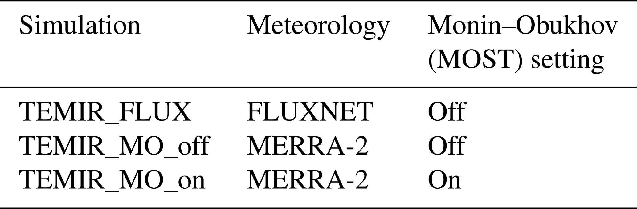
For each of the 49 FLUXNET sites (Table S3) beginning from 2009, simulations shown in Table 1 are conducted for model–observation comparison, with ambient CO₂ concentration kept constant at 390 ppmv. The first set is to use the default surface meteorological fields prescribed from MERRA-2 at 2° × 2.5° horizontal resolution consistent with the GEOS-Chem simulations described above. We also test turning on and off the option of using MOST to infer in-canopy micrometeorological variables from the prescribed meteorology at 2 m above displacement height, as described in Sect. 2.2.4. The second set is to use direct micrometeorological measurements available from the FLUXNET site towers as the driving meteorology and the default MERRA-2 meteorology used only to replace any missing or low-quality data. The results simulated are most relevant for evaluating model performance in reproducing the observed diurnal and seasonal cycle of GPP from each FLUXNET site.

Table 1 TEMIR simulation settings for selected FLUXNET sites.

4.2 Global simulations with TEMIR

Global simulations from 2010 to 2015 are conducted under the same general setup as the site-level simulations, with ambient CO₂ concentration fixed at 390 ppmv and driven by 2° × 2.5° MERRA-2 surface meteorology. A full list of MERRA-2 variables required for running gridded simulations of TEMIR is shown in Table S5. Functionalities of the model are tested for performance, as shown in Table 2, with the MOST option to infer in-canopy conditions and the Sitch O₃ damage scheme with low and high sensitivity to assess the global O₃ impact on vegetation. We use GEOS-Chem (Sect. 2.1) to simulate tropospheric O₃, starting from 2009 to 2015 whereby the first year of simulation is considered as spin-up. The simulation uses the comprehensive chemistry scheme “tropchem”, which has tropospheric O₃–NO_x–VOC–aerosol chemistry accompanied by the default emission inventories (i.e., anthropogenic emissions from CEDS, Hoesly et al., 2018; and biogenic emissions from MEGAN, Guenther et al., 2012). The reanalyzed meteorological fields used are from MERRA-2 supplied by GMAO at 2° × 2.5° horizontal resolution, which are the identical meteorological inputs used in TEMIR. Simulated O₃ concentrations at the lowest surface level are then fed into TEMIR as inputs accordingly. The results produced from these simulations (Table 2) are used to validate the spatial variability in seasonal and annual averages across the whole world against the GOSIF GPP dataset (Sect. 3.2). To retain representative results from all simulations (Table 2), grid cells with LAI < 0.5 are excluded. The transient LAI dataset for the simulation is from MODIS satellite data (Lawrence and Chase, 2007) and assimilated by Yuan et al. (2011). PFT distributional and structural data are regridded to the resolution of MERRA-2 data for TEMIR simulations. We also note that as the model mechanisms are essentially resolution-independent, the model can be straightforwardly modified to conduct simulations at higher resolutions as long as the corresponding input data are provided.

Table 2 TEMIR simulation settings for global simulation for 2010–2015.

4.2.1 Global CO₂–O₃ factorial simulations with TEMIR

We perform factorial simulations (Table 3) to investigate the effects of CO₂ fertilization, O₃ damage, and their interactions on global primary productivity as an example to showcase the utility of the model. Global O₃ surface concentrations of the year 2000 are simulated using GEOS-Chem (Sect. 2.1) with 1999 used as spin-up, and other settings are as described in Sect. 4.2. CO₂ concentrations are changed in TEMIR as required for each simulation (Table 3) with reference to concentrations for 2000 and 2010 (Dlugokencky and Tans, 2022). The Sitch O₃ damage scheme with high sensitivity is used for TEMIR simulations (Table 3) when global surface O₃ concentrations are used as inputs; otherwise, no O₃ damage scheme is used. Meteorological fields for 2000 in MERRA-2 are used for all GEOS-Chem and TEMIR simulations. The LAI is fixed at the year 2000 from MODIS for all GEOS-Chem and TEMIR simulations.

Table 3 Factorial simulation settings. “N/A” for O₃ year indicates that no O₃ damage scheme is used.

5 Model evaluation

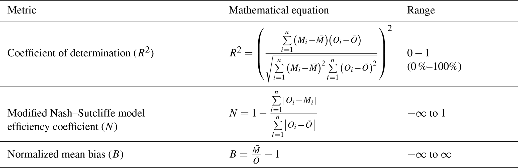
Statistics used for model validation are the adjusted coefficient of determination R², the modified Nash–Sutcliffe model efficiency coefficient N, and the normalized mean bias B. R² is a commonly used metric with a range of 0 to 1 (or 0 %–100 %) that represents the fraction of variability in observations that can be replicated by the model, whereby 1 indicates perfect correlation and 0 indicates no correlation. N addresses the sensitivity issues of R² documented by Legates and McCabe (1999). With values from negative infinity to 1, it is a measure of the suitability of the model as a predictor instead of using the mean of the observations. When N=1, it indicates that the model perfectly replicates observations, and no preference is observed between the model and the mean of the observations as a predictor. Negative values in turn signify the incapability of the model in predicting system behaviors. B gives the relative difference of the magnitude of model results from the observations. The equations to compute these statistics are shown in Table 4.

Table 4 Statistical metrics for TEMIR validation, where M and O respectively represent the simulated dataset and observational dataset, each containing n data points. $\overline{M}$ and $\overline{O}$ represent the means of the datasets in question.

5.1 Site-level validation

5.1.1 Validation on summer diurnal cycle

Figure 1 shows the statistical metrics (Table 4) used to perform a model–observation comparison for the diurnal GPP cycle calculated for each FLUXNET site taken from the second summer month of 2012, which corresponds to the month of July for sites in the Northern Hemisphere and January in the Southern Hemisphere (Table S3). Comparing the simulations with FLUXNET local meteorology and MERRA-2 meteorology (Fig. 1), statistical metrics generally do not differ substantially, but some significant differences can exist for some sites (e.g., CH-Cha and CH-Dav; see Fig. 3) where results from simulations with FLUXNET local meteorology show higher correlations. For simulations solely driven by MERRA-2 meteorology, inferring in-canopy meteorology using Monin–Obukhov similarity theory (Fig. 1c) gives insignificant differences for all sites.

Figure 1 Statistical metrics (see Table 4) for model–observation comparison for the diurnal gross primary productivity from simulations (a) TEMIR_FLUX, (b) TEMIR_MO_off, and (c) TEMIR_ MO_on as described in Table 1.

Figure 2 shows the statistical metrics (Table 4) for model–observation comparison for the simulations using FLUXNET local meteorology as the driving meteorological input for different PFTs. The average correlations per PFT between observed and simulated GPP (Fig. 2) are high (R²>0.88), except for open shrubland (R²≈0.7). B shows a large variability due to various limitations of the model for each PFT. For forest sites, B generally has a smaller range and lower absolute mean values in comparison with the other PFTs, showcasing the better performance of TEMIR for forests. N shows similar behaviors, namely, the prediction for forest sites is satisfactory with mean values of N larger than 0.55, whereas N is mostly negative for grasslands, croplands, and open shrublands. All plots of diurnal cycles are shown in the Supplement, with relevant figures also included in the following discussion.

Figure 2 Statistical metrics (see Table 4) for model–observation comparison for the diurnal gross primary productivity from the TEMIR_FLUX simulation (see Table 1) for each plant functional type listed in Table S1: (a) evergreen needleleaf forest (ENF), (b) evergreen broadleaf forest (EBF), (c) deciduous broadleaf forest (DBF), (d) open shrubland (OSH), (e) grassland (GRA), and (f) cropland (CRO).

We find that the correlations are above 90 % (Fig. 2e) for all grassland sites (e.g., AU-How in Fig. 3a, IT-MBo in Fig. 3b, and CZ-wet in Fig. 3c). Yet the spread of B is large, where we see absolute B values greater than +0.6 for 6 of the 16 sites, and the rest with absolute B less than 0.3. Overestimation of CH-Cha (Fig. 3d) is similar under FLUXNET meteorology, which is likely due to disturbances from intensive site management (i.e., cutting, slurry application, and grazing; Imer et al., 2013; Merbold et al., 2014); this is a shortcoming of simplistic model representation for crops. A possible explanation for the high B values is the fire-prone nature of these sites (i.e., AU-Stp in Fig. 3e) (Beringer et al., 2007, 2011; Hutley et al., 2011; Haverd et al., 2013) whereby the model is incapable of resolving such complexities as turnover and local disturbances. Another cause of overestimation is the simplistic and generic PFT classification for such biomes, which are usually sparsely populated yet with much diversity, as in the open shrubland site ES-LJu (Fig. 3f) (Serrano-Ortiz et al., 2009). Such generalization can also cause systematic inaccuracies in parameterization, where model parameters are better suited for European semiarid vegetation (e.g., CH-Fru, Imer et al., 2013; IT-MBo, Fig. 3b, Marcolla et al., 2011; CZ-wet, Fig. 3c;, Dušek et al., 2012) than similar sites in other regions (e.g., AU-Dry, Hutley et al., 2011; RU-Sam, Fig. 3g, Boike et al., 2013; US-SRG, Scott et al., 2015).

Simulated results for forest PFTs compare very well with observations, where N values are often greater than 0.5. TEMIR performs particularly well for evergreen needleleaf forests as seen in sites DE-Tha (Fig. 3h), FI-Hyy (Fig. 3i), and NL-Loo (Fig. 3j), which are mostly populated by mature Scots pine forests of over 70 years old. Sites CA-TP1 (Fig. 3k), CA-TP3 (Peichl et al., 2010; Arain et al., 2022), and DE-Lkb (Lindauer et al., 2014) are overestimated by the model as these forests are dominated by eastern white pine and Norway spruce that are less than 20 years old, so optimal productivity might not have been achieved. In comparison, the neighboring site CA-TP4 (Fig. 3l; Peichl et al., 2010) with over 70-year-old eastern white pine is better replicated by the model. The model has better performance with respect to site observations when using FLUXNET local meteorology (e.g., CH-Dav in Fig. 3m; Zielis et al., 2014), though the differences are insignificant for most sites. For deciduous broadleaf forest sites, although represented well overall, there is a systematic underestimation (e.g., FR-Fon in Fig. 3n), most likely due to inaccurate parameterization overcompensating for the uncertainties in satellite-derived LAI for broadleaf trees. The multi-year drought in the USA during the 2010s, which hinders plant productivity (Wolf et al., 2016; Xu et al., 2020), appears to improve model agreement by reducing the discrepancy (i.e., US-Oho and US-UMB) and even giving a positive model bias (i.e., US-MMS in Fig. 3o; Yi et al., 2017).

The correlation for croplands is high, but there is a spread in B giving varying N values. The range of model performance among cropland sites shows the limitation of the simplistic crop representation used in this version of TEMIR, whereby site-level settings, such as planting seasons and agricultural management (e.g., fertilizer usage, irrigation, and possible rotations between crop types and cultivars), are not considered. The generic crop representation fails to capture the maximum photosynthetic capacity of the planted crops. For example, site US-Ne1 has irrigated maize that has much higher GPP compared with the simulated generic crop as shown in Fig. 3p. Site DE-Kli (Fig. 3q) has a 5-year crop rotation with occasional fertilizer application (Prescher et al., 2010) and has higher productivity than that simulated by the model.

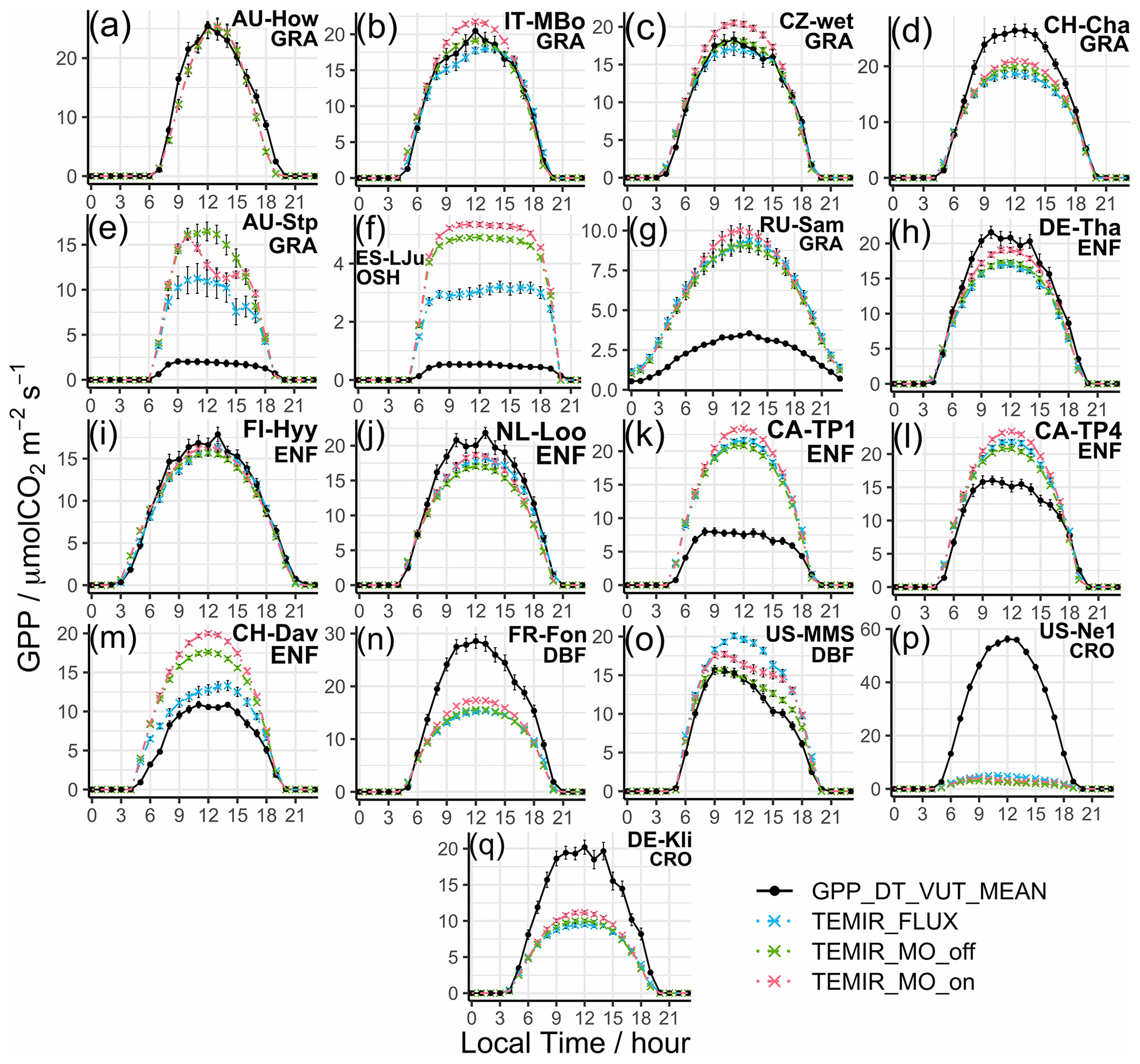
Figure 3 Diurnal averaged gross primary productivity of selected sites representative of their respective vegetation types from simulations described in Table 1, with relevant site information annotated: (a) AU-How, (b) IT-MBo, (c) CZ-wet, (d) CH-Cha, (e) AU-Stp, (f) ES-LJu, (g) RU-Sam, (h) DE-Tha, (i) FI-Hyy, (j) NL-Loo, (k) CA-TP1, (l) CA-TP4, (m) CH-Dav, (n) FR-Fon, (o) US-MMS, (p) US-Ne1, and (q) DE-Kli. More details of these sites are given in Table S3.

5.1.2 Validation on seasonal cycle

Figure 4 shows the statistical metrics (Table 4) for monthly GPP averages of 2009–2013 to examine the model performance in seasonal GPP cycle. All plots of monthly cycles are shown in the Supplement, with plots of selected sites included in the following discussion. The model generally performs worse in capturing the seasonal cycle than the diurnal cycle. Between the different settings of meteorology used for simulations (Fig. 4), the differences in statistics are small. MERRA-2 meteorology shows good utility for most sites, with in-canopy meteorology inferred using Monin–Obukhov similarity theory improving correlation for some sites. FLUXNET local meteorology gives the smallest range of biases with performance similar to MERRA-2 meteorology simulations.

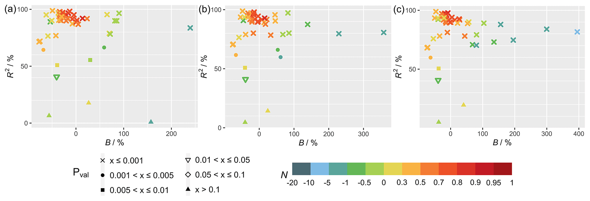
Figure 4 Statistical metrics (see Table 4) of the monthly gross primary productivity from simulations (a) TEMIR_FLUX, (b) TEMIR_MO_off, and (c) TEMIR_MO_on as described in Table 1.

Comparing Figs. 2 and 5, model–observation comparison of monthly averages gives lower values of R² for all sites in general. On the other hand, biases are distributed more evenly across the range with smaller extreme values compared with the biases from diurnal simulations. In terms of N, the model is less adept in reproducing seasonal variations (due to the reductions in correlation) regardless of the driving meteorology chosen. Figure 5c shows that deciduous broadleaf sites (e.g., US-MMS in Fig. 6a) give R²>0.85 with the maximum absolute $B=+\mathrm{0.54}$ and minimum N=0.42 with a mean of 0.9. Monthly performance of forest sites shows a smaller range in B and lower absolute mean values of B in comparison with the other PFTs (Fig. 5). The prediction for forest sites is satisfactory with mean values of N larger than 0.65 (e.g., RU-Fyo in Fig. 6b; CA-TP4 in Fig. 6c), and monthly GPP inaccuracies for forest sites can be explained with similar reasoning as discussed in Sect. 5.1.1.

The correlation for grasslands is above 75 % for most sites (e.g., DE-Akm in Fig. 6d; IT-MBo in Fig. 6e), while sites AU-How (Fig. 6f) and AU-Stp have an R² below 0.4. These sites are known to have fires occurring in the dry winter and spring from May to October, which corresponds to the low productivities (Beringer et al., 2007, 2011; Hutley et al., 2011; Haverd et al., 2013). Moreover, such disturbances on LAI with vegetation regrowth are complex and often overlooked by the model as shown in the simulation of the site AU-How with minimal productivity.

The simulation of monthly GPP of croplands most clearly shows the limitations of the generic model approach, as no site-specific crop phenology is available in this version of the model. The simulated seasonal cycle shows a typical annual peak usually in summer as dictated by meteorology that in general can yield good correlation (e.g., DE-Geb in Fig. 6g); yet, as many sites are intensively managed, the observed GPPs do not follow such a simplistic cycle, giving low correlations (e.g., IT-BCi in Fig. 6h). The parameters for a generic crop usually fail to represent the actual crop planted at the sites, and therefore large biases exist in the simulated GPP (e.g., BE-Lon in Fig. 6i; FR-Gri in Fig. 6j). GPP is more commonly underestimated at the US sites (e.g., US-Ne1 in Fig. 6k) where maize is usually planted and is more productive in comparison with other crops.

Figure 5 Statistical metrics (see Table 4) of the monthly averaged gross primary productivity from the TEMIR_FLUX simulation (see Table 1) for each plant functional type listed in Table S1: (a) evergreen needleleaf forest (ENF), (b) evergreen broadleaf forest (EBF), (c) deciduous broadleaf forest (DBF), (d) open shrubland (OSH), (e) grassland (GRA), and (f) cropland (CRO).

Figure 6 Monthly averaged gross primary productivity of selected sites representative of their respective vegetation types from simulations described in Table 1, with relevant site information annotated: (a) US-MMS, (b) RU-Fyo, (c) CA-TP4, (d) DE-Akm, (e) IT-MBo, (f) AU-How, (g) DE-Geb, (h) IT-BCi, (i) BE-Lon, (j) FR-Gri, and (k) US-Ne1.

5.2 Global validation

Figure 7 shows that the simulated annual averaged GPP for 2010–2015 is 134.7 Pg C yr⁻¹ from the simulation using MERRA-2 meteorology (TEMIR_MO_off) (Fig. 7b), and the simulation with in-canopy meteorology inferred using MOST (TEMIR_MO_on) gives GPP over the same period as 144.7 Pg C yr⁻¹ (Fig. 7c). Compared with the satellite-derived dataset (GOSIF GPP; Sect. 3.2) where the annual GPP of the same period is 128.4 Pg C yr⁻¹ (Fig. 7a), TEMIR overestimates global GPP by ∼ 5 %–10 % depending on the input meteorology (Table 5). TEMIR performance is well within, and leans toward, the middle of the observation-constrained range in the literature of 119–175 Pg C yr⁻¹. TEMIR closely agrees with models of similar design objectives, e.g., the Yale Interactive terrestrial Biosphere (YIBs) with GPP at 125±3 Pg C yr⁻¹ (Yue and Unger, 2015) and JULES land surface model estimating GPP at 141 Pg C yr⁻¹ (Slevin et al., 2017). TEMIR can largely reproduce the spatial distribution of GPP with respect to GOSIF GPP (Fig. 7), with grid cells with mixed savanna and forests showing larger discrepancies.

Table 5 Gross primary productivity (GPP) product simulated and relevant simulation details of global TEMIR simulations described in Tables 2 and 3. “N/A” for O₃ year indicates that no O₃ damage scheme is used.

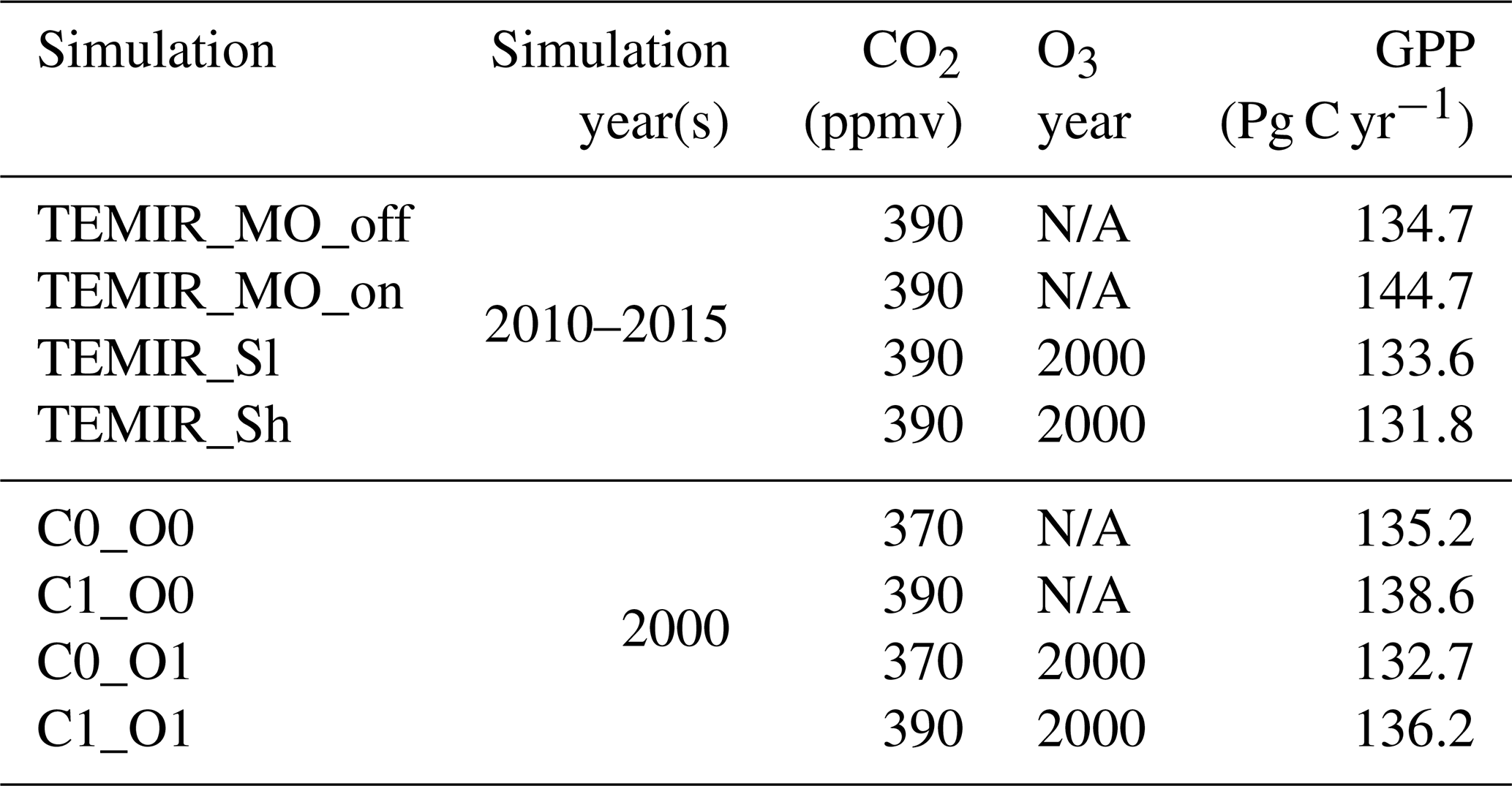
Figure 8 shows model–observation statistics (Table 4) for the model outputs of Fig. 7 in 12 regions. Global correlation of 6-year averaged GPP is around 83 % (Fig. 8b). In general, correlations are lower for regions closer to the Equator, where correlations for tropical regions are below 70 % but otherwise above 70 %, with correlation for Siberia close to 90 %. Correlation for the tropical Americas is ∼ 75 %, which is higher than other equatorial regions. Temperate North America shows a correlation of ∼ 60 %, which is lower than other regions at midlatitudes. We also see that GPP is underestimated in the grid cells with high crop density (Fig. 7b), which, as discussed in Sect. 5.1, is likely due to the generic crop representation of the TEMIR version giving poor model performance for this region. Simulated GPP driven by meteorology inferred with MOST gives small increases or decreases in regional correlation (e.g., correlation for North Africa and the Middle East drops from 48 % to 45 %, and correlation for temperate South America increases from 75 % to 78 %).

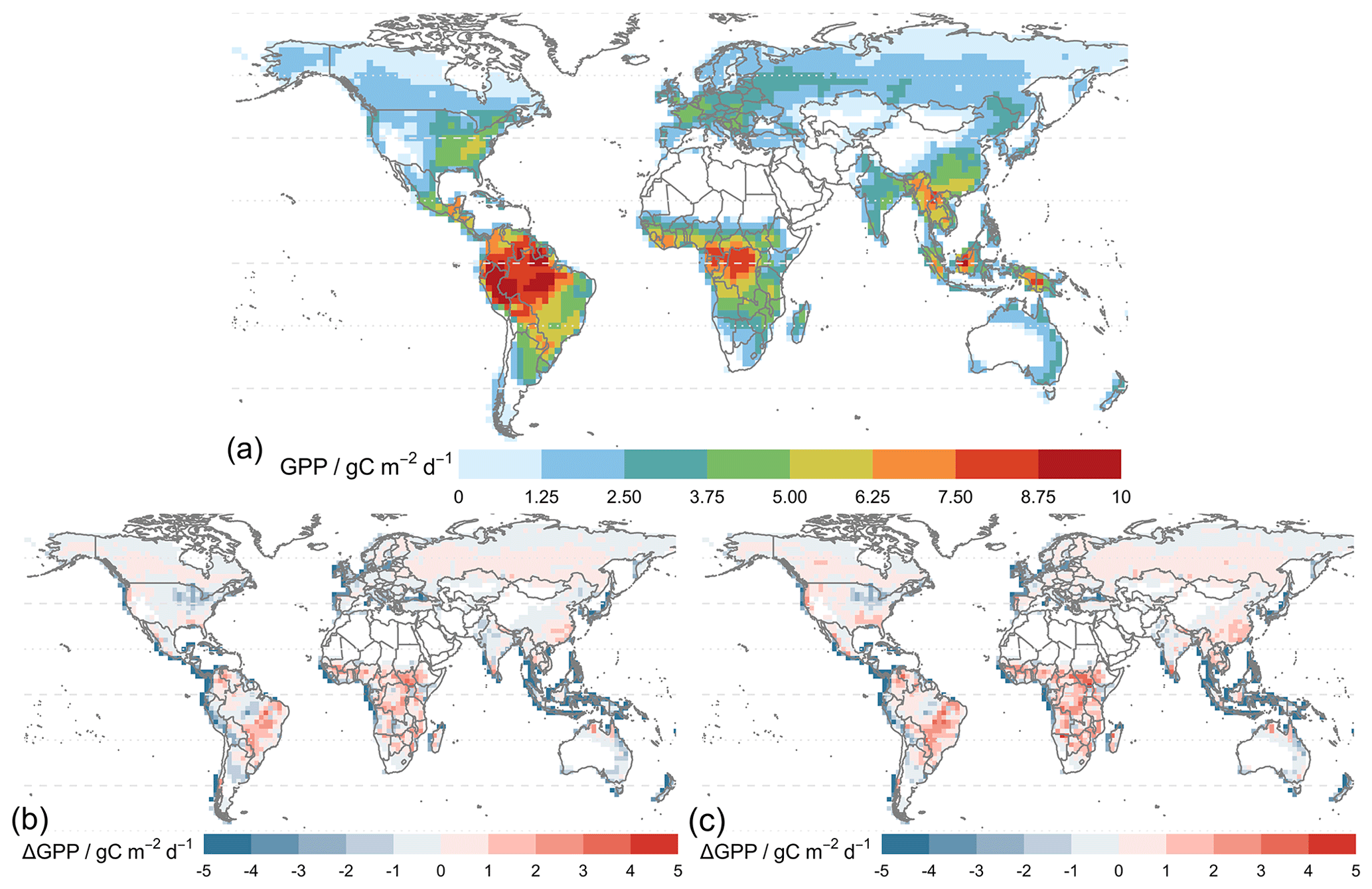
Figure 7 Panel (a) shows the average global gross primary productivity for 2010–2015 from the GOSIF GPP product and differences in the simulated GPP from simulations. Panel (b) shows TEMIR_MO_off and (c) shows TEMIR_MO_on (see Table 1) for 2010–2015 compared with the GOSIF product.

Absolute biases are mostly within 25 % except for North Africa, the Middle East, and sub-Saharan Africa (except central Africa) when the driving meteorology is inferred from MOST. Simulated GPP driven by in-canopy meteorology inferred with MOST gives more positive biases for all regions, generally around +10 %. GPP for 6 of the 12 regions is overestimated by TEMIR and otherwise underestimated (Fig. 8b). Thus, in-canopy meteorology inferred with MOST results in regional bias changes from underestimation to overestimation for East and South Asia, Europe, temperate North America, and the tropical Americas. The bias for Europe is −6.2 % and +1.19 % when driving meteorology is inferred with MOST. The bias of +1.19 % is the smallest absolute bias of any region, which shows the possibility of in-canopy meteorology inferred with MOST improving GPP predictions for some but not all regions.

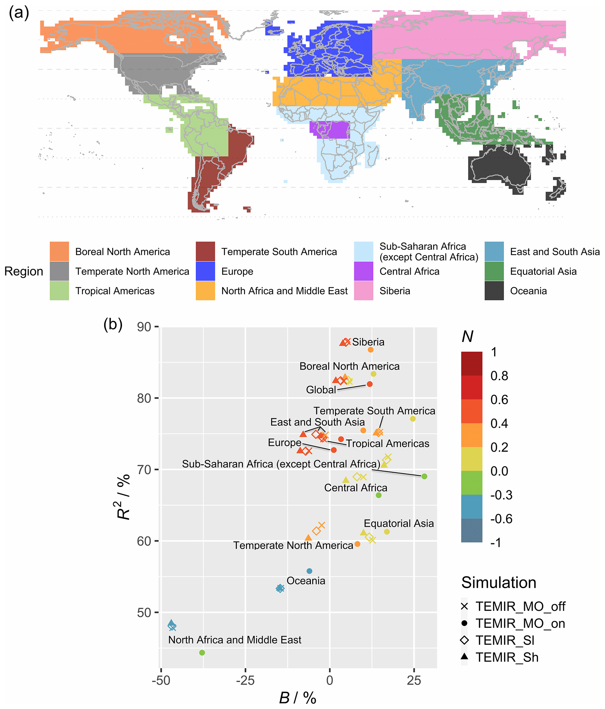
Figure 8 Panel (a) shows regional division relevant for this study largely following Chen et al. (2017), and (b) shows the corresponding regional statistical metrics (see Table 4) of the averaged gross primary productivity for 2010–2015 from TEMIR simulations (see Table 2).

5.3 Effects of O₃ and CO₂ on global primary productivity

Figure 9 shows the simulated results where the Sitch O₃ schemes (Sect. 2.2.5) of low sensitivity (Sl) and high sensitivity (Sh) are implemented for 2010–2015 using MERRA-2 meteorology. Figure 9a shows the mean daily 8 h averaged O₃ concentration (MDA8), a common surface O₃ metric, derived from the simulated hourly O₃ concentration at the lowest model level affecting global vegetation under the Sitch O₃ damage scheme. The global GPP values are 133.6 and 131.8 Pg C yr⁻¹ for the Sitch O₃ scheme at low and high sensitivity, respectively (Table 5), both of which are smaller than the 134.7 Pg C yr⁻¹ from the simulation without O₃ damage (Fig. 7b). These global GPP reductions are seemingly small (< 1 % to ∼ 2 %) and conceal larger regional changes. Figure 9c shows that the Sitch O₃ damage scheme at high sensitivity leads to an up to 15 % reduction in GPP, whereas low sensitivity shows modest reductions of about half of those magnitudes. Particularly large O₃-induced damage occurs in highly populated regions (e.g., the eastern USA, Europe, central Africa, northern India, and East Asia) associated with high anthropogenic emissions (NO_x in particular). Many of these regions also contain arable lands, and thus O₃ exposure can also affect food security (Feng et al., 2008; Avnery et al., 2011; Emberson et al., 2018; Ainsworth et al., 2020; Tai et al., 2021; Leung et al., 2022; Roberts et al., 2022).

Figure 8b shows the statistics of Table 4 per region (Fig. 8a) for simulations with O₃ damage. The presence of O₃ does not affect the model–observation correlations significantly for any region. When compared with the correlations of TEMIR_MO_off simulation results, correlations from O₃-damaged GPP show small differences. O₃ damage reduces the model overestimation with respect to GOSIF GPP. In particular, for eastern China and central Africa, implementing O₃ damage reduces the positive model biases as seen in Fig. 7. Underestimation is worsened for the regions of temperate North America as well as East and South Asia where there is strong O₃ damage (Fig. 9).

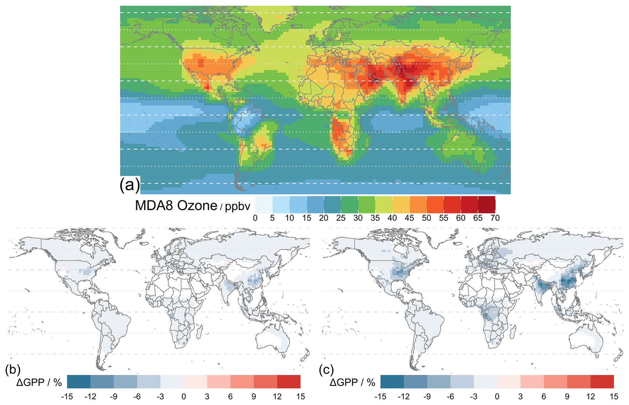
Figure 9 Mean daily 8 h averaged (MDA8) O₃ concentration of the lowest model layer averaged over 2010–2015 and percentage differences in average global GPP for 2010–2015 of the simulated results with the Sitch O₃ damage scheme at (b) low sensitivity and (c) high sensitivity from the simulation TEMIR_MO_off (see Table 2).

Figure 10 shows the comparisons between simulations (Table 3) displaying the interplay of CO₂ fertilization effects and O₃ damage to GPP. CO₂ fertilization (from 370 to 390 ppmv), shown in Fig. 10b, promotes regional productivity by up to 7 %. Global GPP enhancement is ∼ 2 % (Table 5), and thus simulations estimate that rising atmospheric CO₂ concentration results in a global GPP increase of 0.126 % ppmv⁻¹. As seen in Fig. 10c, O₃-induced regional reductions are up to 15 % under the Sitch O₃ damage scheme at high sensitivity, whereby results are similar to those in Fig. 9c. Figure 10d shows the differences in percentage of O₃ damage to GPP of the simulation with O₃ damage at a CO₂ concentration of 390 ppmv from that at 370 ppmv (i.e., that of Fig. 9c). The positive values in Fig. 10d indicate that the O₃-induced GPP reduction is smaller at a higher CO₂ concentration, reflecting the additional benefits of CO₂ fertilization from the reduced stomatal conductance, which improves water use efficiency and also decreases stomatal O₃ uptake thus lessening O₃-induced impacts.

Figure 10 Plots showing results from simulations of Table 3: (a) gross primary productivity modeled for 2000 at a CO₂ concentration of 370 ppmv (C0_O0), (b) percentage changes in GPP showing CO₂ fertilization effects of year-2010 CO₂ concentration at 390 ppm (100 % × (C1_O0 − C0_O0)$/$C0_O0), (c) percentage changes in GPP due to O₃ damage at high sensitivity of the Sitch O₃ damage scheme for year-2000 modeled O₃ concentration and CO₂ concentration of 370 ppmv (100 % × (C0_O1 − C0_O0)$/$C0_O0), and (d) differences in percentage of O₃ damage at a CO₂ concentration of 390 ppmv from that at 370 ppmv (100 % × (C1_O1 − C1_O0)$/$C1_O0 − 100 % × (C0_O1 − C0_O0)$/$C0_O0), whereby positive values indicate a reduction in percentage of O₃ damage.

6 Discussion and conclusions

In this paper we provide a detailed model description of the newly developed Terrestrial Ecosystem Model in R (TEMIR) version 1.0, which simulates ecophysiological processes and functions (most importantly, photosynthesis and global primary productivity) of terrestrial ecosystems as represented by different PFTs, driven by prescribed meteorological conditions and atmospheric chemical composition. We specifically include the multiple parameterization schemes for stomatal O₃ uptake and O₃ damage to plants, as well as showcasing the utility of TEMIR in evaluating the responses of GPP to O₃ damage, CO₂ fertilization, and their interactions. The productivity simulated at site and global levels reproduces the observed diurnal and seasonal cycles well for evergreen needleleaf and deciduous broadleaf forests (especially those that are mature), with an annual average GPP of 134.7 Pg C yr⁻¹ for 2010–2015 and a global reduction of up to 2 % when O₃ damage is considered. This is validated against the productivity from the 49 FLUXNET sites and GOSIF GPP.

TEMIR-simulated global GPP lies well within the accepted range, but the associated large uncertainty is well acknowledged in the field (Bonan et al., 2011; Baldocchi et al., 2016; Zhang et al., 2017; Li and Xiao, 2019; Bi et al., 2022; Wild et al., 2022; Zhang and Ye, 2022), thus limiting the validity of global GPP model–observation comparison in this study (Sect. 5.2). Site-level validation may lend more credence by isolating certain PFTs for comparison, albeit being more limited in scope and scale unlike global comparisons. Our investigation suggests that possible PFT systematic biases exist generally for diurnal productivity, which reflect the limitations of having a set of prescribed parameters for generalized classes of plant functions (Harrison et al., 2021; Seiler et al., 2022; Liu et al., 2023; Wu et al., 2023a). For instance, there is a systematic underestimation for deciduous broadleaf forests, though it can be explained by the uncertainties in LAI datasets (Liu et al., 2018; Yang et al., 2023), and some regions show distinctive physiology and phenology of grasses and shrubs. Particularly for semiarid regions where the range of productivity is large, the model shows variable accuracy. In general, variability in prescribed LAI can be an important source of uncertainty in the model results. Single-site sensitivity simulations show that GPP generally linearly increases with LAI at low LAI, but as LAI becomes larger, GPP increases less than proportionately due to the canopy shading effect. Such nonlinearity of GPP responses to LAI changes is less important for small perturbations of LAI (e.g., < 20 %).

Simulating crops in ecosystem modeling remains particularly challenging (Deryng et al., 2016; Chopin et al., 2019; Muller and Martre, 2019; Boas et al., 2021), as it combines the nuances in phenology, physiology, coverage, and active human management with high spatiotemporal variations (Monfreda et al., 2008; Emberson et al., 2018; Ahmed et al., 2022; Gleason et al., 2022; Corcoran et al., 2023), which already exist for natural vegetation to a lesser degree. One particularly crucial aspect for improvement is to get crop LAI correct, which is typically more challenging to measure than trees with large canopies and often varies to greater extents with leaf orientations for different crops. More long-term ground-based and/or remote sensing measurements of crop LAI for different crop types across the world are particularly recommended, not only as input data but also for model validation in future development. Especially for site-level simulations, locally relevant crop physiological and structural parameters should also be measured and used. Ongoing development has already been attempting to enhance crop representation in a version of TEMIR with active crop biogeochemistry (Tai et al., 2021) to improve and reconcile model inaccuracies.

Incorporating site-level meteorology in simulations can improve performance for a few selected sites but otherwise is comparable to results from simulations with gridded assimilated meteorology as input. This highlights the fact that generalization and the coarse resolution of the MERRA-2 dataset used (due to computational limitations and necessary consistency with other input datasets) can drastically overlook regional and small-scale nuances. Furthermore, CO₂ concentration was kept constant and spatially uniform in all simulations, which enables direct comparison with other modeling studies but ignores possible spatiotemporal variability in CO₂ concentration (Cheng et al., 2022). Though such effects are usually minor on simulated GPP magnitudes (Lee et al., 2018; Tian et al., 2021), uncertainties should be minimized in any case; thus, it is recommended that users use the measured CO₂ concentration, if available, as input, especially for site-level simulations. It is also recommended that users recalibrate relevant model parameters with site observations and available datasets (e.g., those of higher resolutions), such as LAI, V_cmax, PFT fractional coverage, and others, to yield the most accurate results. The non-dynamic representation of vegetation cover and parameterization is a shortcoming of TEMIR, and thus simulations overlook intricate and transient impacts of LULCC on land–atmosphere exchange (Ganzeveld et al., 2010; Pongratz et al., 2010; Prescher et al., 2010; Chen et al., 2018; Bastos et al., 2020; Hou et al., 2022). With the capacity of the current version of TEMIR, our simulations address these aspects by changing the input data of LAI and PFT fractions, derived from LULCC, for yearly and higher frequencies. LULCC can drive large regional changes, though recent LULCC mostly reduces GPP (due to urbanization, agricultural expansion, and deforestation), counteracted partly by CO₂ fertilization effects (Wu et al., 2023b), and thus the validity of our results is likely unchanged. The assumption of sufficient nitrogen availability is a limitation (Sandor et al., 2018) as most non-tropical biomes experience varying nitrogen limitation (Davies-Barnard et al., 2022; Kou-Giesbrecht and Arora, 2023), thereby affecting photosynthetic capacities (Mason et al., 2022; Wang et al., 2022) and resource allocations in plants and soil (Zhang et al., 2020; Feng et al., 2023; Lu et al., 2023). Some models have N cycling (Yang et al., 2009; Gerber et al., 2010; Wiltshire et al., 2021; Hidy et al., 2022), but effects remains minor (Jain et al., 2009; O'Sullivan et al., 2019; Lin et al., 2023) in the recent decade and more relevant for assessing future global changes (Tharammal et al., 2018; Franz and Zaehle, 2021). Overall, TEMIR has great skill in capturing annual and seasonal GPP at the global scale as well as for some productive regions and certain PFTs, whereby the correlation is high in the range of 80 %–90 %, showcasing the utility of TEMIR at different scales. Caution should be taken with good knowledge of model preferences and the underlying theoretical assumptions for any given research question, especially when concerning multi-factor land–atmosphere interactions and vegetation responses to various environmental stresses (Kimmins et al., 2008; Zhao et al., 2022; Blanco and Lo, 2023; Rahman et al., 2023). Further development and validation of the model with detailed observations are crucial to provide more accurate vegetation parameterization for specific applications, e.g., to investigate vegetation responses to droughts and heatwave composition (e.g., Yan et al., 2022), especially at the regional and site levels.

The initial motivation and one of the most relevant applications of TEMIR is to address the impacts of O₃ pollution and exposure on terrestrial ecosystem productivity, whereby an active Sitch O₃ damage scheme improves model performance with respect to GPP. Concerning O₃ damage to GPP, there is good agreement with previous studies in terms of both magnitudes and spatial variations (e.g., Lombardozzi et al., 2015; Sitch et al., 2007). For instance, the OCN model (Franz et al., 2017; Franz and Zaehle, 2021) simulated O₃ as reducing GPP in Europe by ∼ 8 % and the JULES land surface model (Slevin et al., 2017) in the range of 10 %–20 % (Oliver et al., 2018). The Yale Interactive terrestrial Biosphere (YIBs) model (Yue and Unger, 2015) simulated O₃ as reducing global GPP by 2 %–5 % with East Asia experiencing damage of 4 %–10 %. Yue and Unger (2014) also showed GPP reductions of 4 %–8 % in the eastern USA with high episodes giving a higher range of 11 %–17 %. YIBs has the capability of synchronous coupling (e.g., GEOS-Chem–YIBs; Lei et al., 2020), which reported similar ranges in GPP reductions: globally by 1.5 %–3.6 % and extremes of 11 %–14 % in the eastern USA and eastern China. This lends credence to the comparable performance of TEMIR v1.0, which has a more simplistic terrestrial ecosystem with prescribed ecosystem structure (noting that active biogeochemistry is in development).

O₃ influences in the current version of TEMIR are limited to vegetation physiological and productivity responses. Intra- and interspecies differential sensitivity to O₃ can cause competition (Agathokleous et al., 2020), affecting some species more than others in terms of biomass, flowering, and seed development, thus impacting community composition, PFT fractional coverage, and biodiversity (Calvete-Sogo et al., 2016; Fuhrer et al., 2016; Emberson, 2020). This can also be seen among functional groups. For example, perennial species retain more aboveground biomass than annual species, and angiosperms are more prone to O₃ damage than gymnosperms, thus giving possible long-term biodiversity effects (Agathokleous et al., 2020). Such effects are further complicated by soil conditions (e.g., water and nitrogen content) and also spatial heterogeneity, whereby regional strategies might differ within functional groups, although this requires more studies to obtain observation-based parameterization.

Moreover, synchronous model coupling between a CTM or climate model and a fully prognostic biosphere model with active biogeochemistry is particularly suitable for examining O₃–vegetation feedbacks (Danabasoglu et al., 2020; Franklin et al., 2020; Lam et al., 2023), especially for timescales long enough (e.g., multi-decadal) for ecosystem structure to co-evolve with the atmosphere. For instance, Sadiq et al. (2017) and Gong et al. (2021) showed that dynamic O₃–vegetation interactions can lead to a long-term ecosystem decline and a positive feedback on O₃ concentration in China and worldwide, respectively, worsening air quality. Zhu et al. (2022) and Jin et al. (2023) found similar positive O₃–vegetation feedbacks in China with the coupled framework using WRF-Chem and Noah-MP. Yue et al. (2017) also investigated O₃–aerosol–vegetation interactions in China. TEMIR can only be asynchronously coupled with GEOS-Chem and is not the best tool for investigating two-way O₃–vegetation interactions, especially when such interactions relevantly happen within a model time step, but it is particularly suitable for estimating first-order effects of O₃ pollution on vegetation in a computationally efficient manner. Zhou et al. (2018) indeed found that second-order effects of O₃ pollution (i.e., additional effects of modified O₃ concentrations after feedbacks are accounted for) on vegetation are negligible. Moreover, asynchronous coupling between TEMIR and GEOS-Chem, for example, and conducting factorial experiments with them, can help disentangle complex pathways and feedbacks that are often convoluted in fully coupled models.

We recognize that the O₃ damage scheme in TEMIR does not account for sluggishness in stomatal responses (e.g., Clifton et al., 2020; Huntingford et al., 2018), which may modify further O₃ uptake, although such effect is expected to be small at the resolution relevant for this study. O₃ sensitivities also have crop-related inaccuracies due to the generic crop representation in this version of TEMIR. Such is a common practice in global-scale biosphere models, and Leung et al. (2020) suggested that if a study focuses on crop yields, species-specific calibration is required to reduce uncertainty and likely inaccuracies for the crops concerned. TEMIR v1.0 on a global scale is not suitable for any crop-focused investigations, but one may use the version of TEMIR implemented with additional crop functionalities, such as the calculation of phytotoxic O₃ dose, taking advantage of the stomatal calculation in TEMIR and the subsequent estimation of O₃–crop impacts (Tai et al., 2021). The utility of TEMIR in examining vegetation-mediated dry depositional sinks of O₃ has also been demonstrated (Sun et al., 2022).

Mechanistic representations allow modeling for various meteorological conditions and are extremely useful to evaluate ecophysiological responses to a changing climate and intermittent climate extremes (e.g., Bonan, 2008, 2016; Cai and Prentice, 2020; Gang et al., 2022). Ciais et al. (2005) estimated a 30 % GPP reduction in Europe following the heatwave in 2003 and vegetation there became a net carbon source, attributable to the rainfall deficit and extreme summer heat. This was also found by Bamberger et al. (2017), whereby heat and drought impacts alter photosynthesis and vegetation state. More extreme events are projected for a future climate, which various models (e.g., O-CN and YIBs) have shown to decrease productivity (e.g., Franz and Zaehle, 2021; Yan et al., 2022). He et al. (2022), using models, showed that climate variability is the main factor controlling interannual GPP variability in grasslands in China. Such effect is the most prominent in summer, which is responsible for more than 40 % of decadal GPP variability in Chinese grasslands and the largest in comparison with effects from CO₂ fertilization and nitrogen deposition. Similar to the case for O₃–vegetation coupling discussed above, fully coupled climate–biosphere models can be particularly useful for examining two-way interactions and feedbacks and also long-term (multi-decadal to multi-centurial) co-evolution of climate and the biosphere. However, the embedded complex interactions may obscure the relative importance of different factors, making it a lot more difficult to attribute changes to specific factors. Offline modes, such as TEMIR, are therefore particularly useful for investigating and attributing biospheric variability and changes to prescribed changes in climatic variables.

In addition, we have demonstrated the utility of TEMIR in examining the direct and interactive effects of multiple atmospheric chemical species on global vegetation (i.e., CO₂ and O₃ concentrations). CO₂ fertilization in TEMIR results in strong GPP enhancement as seen in many studies (e.g., Schimel et al., 2015; Cai and Prentice, 2020; Chen et al., 2022; Yang et al., 2022). Our simulations estimate that CO₂ fertilization increases global GPP by 0.126 % ppmv⁻¹, which is comparable to the value of 0.138 % ± 0.007 % ppmv⁻¹ reported by Ueyama et al. (2020). It is noteworthy that some studies (e.g., Lee et al., 2018) suggest that overlooking spatiotemporal variability in atmospheric CO₂ can lead to inaccuracies in seasonal and regional GPP estimation but only a minor influence on global GPP. Additional crop functionalities of TEMIR (Tai et al., 2021) can also address the CO₂ fertilization effects on crops, although studies have also found that the resultant productivity increase gives larger yield quantity but does not necessarily translate to increased yield quality (Myers et al., 2014; Ebi et al., 2021; Xia et al., 2021). The competing effects of CO₂ fertilization and O₃ damage to vegetation have been well documented in field experiments, although magnitudes vary and are species-dependent (e.g., Oikawa and Ainsworth, 2016; Proietti et al., 2016; Karlsson et al., 2017; Moura et al., 2018; Zhang et al., 2018; Ainsworth et al., 2020; Xia et al., 2021). TEMIR shows that CO₂ fertilization can reduce the percentage of O₃ damage to vegetation (∼ 1 % globally), which is generally comparable to 1 %–2 % found by Oliver et al. (2018), whereas Sitch et al. (2007) simulated a higher range of 6 %–9 %. We note that while comparisons among models are useful, we must be mindful of the differences in model designs and setups (as mentioned in Sect. 1). Miner et al. (2017) cautioned that stomatal responses to CO₂ can be highly species-dependent and variable under different soil conditions, adding more uncertainty to the parameterization of CO₂–O₃–vegetation interactions. The changing nitrogen deposition due to anthropogenic activities may likewise influence the interactions between vegetation, CO₂, and O₃ (Zhao et al., 2017; Liu et al., 2021), whereby nitrogen can limit CO₂-promoted growth (Wang et al., 2020) or modify vegetation responses (e.g., for g_s; Hu et al., 2021) with further implications on soil and nutrient cycling (Terrer et al., 2021). As atmospheric composition rapidly changes in the next century, these interactive mechanisms should be considered for modelers to more representatively and accurately model the future earth system (e.g., Bytnerowicz et al., 2007; Pu et al., 2017; Sicard et al., 2017; Franz and Zaehle, 2021; Leung et al., 2022).

All in all, the high adaptability of TEMIR, written in an freely open-source, widely used, and easy-to-learn programming language (R Core Team, 2022), is expected to facilitate fruitful contribution to research, at various spatiotemporal scales, on biosphere–atmosphere interaction. It also provides a readily available tool for policymakers, practitioners, and other stakeholders to assess the ecosystem services provided by vegetation in different regions or cities, as well as their sensitivities to future atmospheric changes, possibly enhancing the translational value of ecological and geoscientific research.