the Creative Commons Attribution 4.0 License.
the Creative Commons Attribution 4.0 License.
 | 03 May 2024
Assimilation of GNSS tropospheric gradients into the Weather Research and Forecasting (WRF) model version 4.4.1
Rohith Thundathil
Florian Zus
Galina Dick
Jens Wickert
In this study, we have incorporated tropospheric gradient observations from a Global Navigation Satellite Systems (GNSS) ground station network into the Weather Research and Forecasting (WRF) model through a newly developed observation operator. The experiments aim at testing the functionality of the developed observation operator and at analyzing the impact of tropospheric gradients on the sophisticated data assimilation (DA) system. The model was configured for a 0.1° mesh over Germany with 50 vertical levels up to 50 hPa. Our initial conditions were obtained from the National Centers for Environmental Prediction (NCEP) Global Forecast System (GFS) data at 0.25° resolution, and conventional observations were obtained from the European Centre for Medium-Range Weather Forecasts (ECMWF), restricted to mainly surface stations and radiosondes. We selected approximately 100 GNSS stations with high data quality and availability covering Germany. We performed DA every 6 h for June and July 2021. Four experiments were conducted: (1) a control run assimilating only conventional observations; (2) an impact run assimilating zenith total delays (ZTDs) on top of the control run; (3) an impact gradient run assimilating ZTDs and gradients on top of the control run; and (4) a gradient run assimilating only gradients on top of the control run. The error for the impact run was reduced by 32 % and 10 % for ZTDs and gradients, whereas the error for the impact gradient run was reduced by 35 % and 18 %, respectively. The gradient errors for the gradient run were nearly equal to those of the impact gradient. Overall, the newly developed operator for the WRFDA system works as intended. In particular, the combined assimilation of gradients and the ZTDs led to a notable improvement in the humidity field at altitudes above 2.5 km. With the operator codes developed and freely available to the WRF users, we aim to trigger further GNSS tropospheric gradient assimilation studies.
- Article
(10655 KB) - Full-text XML
- BibTeX
- EndNote


Water vapor, one of the vital components in the atmosphere, plays a crucial role in weather forecasting and climate research. It is the most abundant greenhouse gas, which accounts for 70 % of atmospheric warming and plays a vital role in energy exchange within the atmosphere. However, more knowledge is needed about the humidity field due to limited observations and sub-optimal data assimilation (DA) systems. To ensure effective weather forecasting, it is imperative to have precise and uninterrupted observations that serve as the basis for initializing numerical weather prediction models. The spatio-temporal distribution of water vapor information is crucial for accurate modeling of the atmosphere. This is especially important for predicting heavy precipitation and severe weather events, which are among the most critical challenges in weather research.
Global Navigation Satellite Systems (GNSS) has profoundly transformed how we determine our position, navigate, and keep track of time. Apart from positioning and timing applications, GNSS is a powerful and versatile tool for geosciences. It can accurately sense atmospheric temperature, water vapor content, ionospheric electron content, Earth surface properties, deformation, and other geophysical parameters (Wickert et al., 2020).
A crucial aspect of geophysics involves monitoring atmospheric water vapor using GNSS regional ground networks. This helps to fill gaps in established meteorological observing systems. For instance, Germany currently operates around 270 stations. No other observation network has such a high temporal and spatial resolution. However, there is room for improvement in the impact of the currently provided zenith total delay (ZTD) data products on forecast systems due to limited atmospheric information content.
GNSS satellites transmit radio signals that ground-based stations receive to estimate ZTDs and tropospheric gradients. This capability was initially demonstrated by Bevis et al. (1992) for ZTDs and by Bar-Sever et al. (1998) for tropospheric gradients. GNSS meteorology relies on ZTD, which is the core observable strongly correlated with integrated water vapor (IWV) above the station. GNSS stands out among other observation systems for its numerous benefits, including low operating expenses, all-weather availability, and exceptional spatio-temporal resolution. ZTD data are readily accessible from multiple station networks in Europe, such as the European Meteorological Services Network GNSS Water Vapor Program (E-GVAP), in near real time. E-GVAP was established in April 2005 to provide near-real-time GNSS delay data. These data contain information about the amount of water vapor above GNSS sites. The meteorological data provided by E-GVAP can validate GNSS delay estimation and enhance GNSS positioning in the future. Currently, the E-GVAP network comprises over 3500 GNSS sites. Studies on assimilation have demonstrated that using ZTD data enhances forecast accuracy, as shown in the findings of Vedel and Huang (2004). Poli et al. (2007) utilized a four-dimensional variational (4D-Var) data assimilation technique to assimilate GNSS ZTD data into the Action de Recherche Petite Échelle Grande Échelle (ARPEGE) global model, positively impacting the assimilation of synoptic-scale circulations and precipitation forecasting during spring and summer. Further research in France by Boniface et al. (2009) and Yan et al. (2009) validated the beneficial influence of incorporating GNSS ZTD data into the NWP model. Lindskog et al. (2017) performed GNSS ZTD DA using the HIRLAM–ALADIN (High Resolution Limited Area Model; Aire Limitée Adaptation Dynamique Développement International) Research on Mesoscale Operational NWP in Euromed (HARMONIE) Applications of Research to Operations at Mesoscale (HARMONIE–AROME) model at a 2.5 km horizontal resolution, indicating that incorporating GNSS ZTD as an additional observation type improves forecast quality and highlights the potential for further improvements in DA through the integration of GNSS ZTD with other observation types. In a study by Rohm et al. (2019), GNSS data were incorporated into the Weather Research and Forecasting (WRF) model at a 4 km horizontal resolution over Poland for 2 months, revealing a significant enhancement in the model's ability to forecast both water vapor and precipitation. Studies by Giannaros et al. (2020) and Caldas-Alvarez and Khodayar (2020) demonstrate the significant benefits of GNSS ZTD DA in improving precipitation and water vapor forecast accuracy, focusing on Greece and a broader Mediterranean and central European region, respectively. Lagasio et al. (2019) discovered that incorporating diverse Sentinel-1 and GNSS ZTD observations into the WRF model offers the most significant advantages to forecasts by providing details on the wind field and water vapor content. Mascitelli et al. (2019, 2021) successfully used the RAMS@ISAC model in two experiments to assimilate GNSS ZTD and IWV data. GNSS ZTD was assimilated using a three-dimensional variational (3D-Var) data assimilation technique, while IWV was assimilated through nudging. This assimilation led to a notable improvement in short-term water vapor prediction, while having a minor effect on precipitation forecasts in both instances.
Several European weather agencies assimilate ZTD data. However, their utility is limited because they do not provide information on horizontal or vertical atmospheric gradients (Bennitt and Jupp, 2012; Mahfouf et al., 2015). Tropospheric gradients have the potential to offer valuable additional insights. Until now, most studies have primarily focused on validating tropospheric gradients. Bar-Sever et al. (1998) initially reported preliminary findings confirming genuine atmospheric features in tropospheric gradients. However, their study compared data from only one station to tropospheric gradient estimates obtained from a collocated water vapor radiometer for assessing tropospheric gradients. Subsequently, the exploration of tropospheric gradients gained traction in meteorology. One of the early efforts was by Walpersdorf et al. (2001), who compared tropospheric gradients derived from GPS with those obtained from a numerical weather model (NWM) for a specific set of stations. Iwabuchi et al. (2003) demonstrated a strong correlation between tropospheric gradients and the moisture field. Typically, tropospheric gradients, when plotted as vectors, indicate the direction from dry to moist regions, as noted by Brenot et al. (2013) in their investigation of deep convection. Li et al. (2015) showed that improving the observation geometry leads to more accurate estimations of tropospheric gradients. Morel et al. (2015) conducted a study on tropospheric gradients using various software packages to analyze data from 12 stations on Corsica, a Mediterranean island. However, it is noteworthy that these studies often involve a limited number of stations. Douša et al. (2016) compared multiple stations and two GNSS analysis techniques with tropospheric gradients from NWMs. Their visual inspection of tropospheric gradient maps provided compelling evidence that GNSS tropospheric gradients accurately capture actual tropospheric features. While they made positive findings, certain aspects required further exploration, such as understanding the role of GNSS data processing options and parameters. During the second Reference Frame Sub-Commission for Europe (EUREF) reprocessing, Dousa et al. (2017) identified distinct artificial signals in tropospheric gradients, attributed to the absorption of asymmetric effects resulting from instrumentation issues. They also noted seasonal variations in deviations between GNSS and NWM ZTDs and tropospheric gradients, with larger deviations observed in summer due to NWMs struggling to predict high water vapor variability. The data suggests that while the standard deviation for ZTDs remained consistent over time, the standard deviation for tropospheric gradients decreased, indicating improved quality over the years. Since their introduction in the early 1990s, GNSS ZTDs have consistently maintained high quality in meteorology. Kačmařík et al. (2019) studied the sensitivity of tropospheric gradients to various processing options and found that post-processing mode solutions reliably estimated tropospheric gradients correlating well with actual weather conditions. The accuracy of real-time tropospheric gradient estimates primarily depends on the availability of high-quality satellite orbits and clocks. The purpose of this study is to advance a step further by making use of tropospheric gradients. One possibility is to assimilate tropospheric gradients into an NWM, requiring the development and implementation of observation operators into DA systems. This research incorporated a new observation operator in the WRFDA system, which allows one to assimilate GNSS tropospheric gradients.
The developed operator is an upgrade or an add-on to the current ZTD operator already implemented in the WRFDA. Hence, the modules connected with the ZTD operator codes were modified with additional code snippets to create the ZTD+gradient version of the operator. Users can quickly assimilate gradients with this operator by adding a few lines to the WRFDA namelist.input. The process can be controlled with switches in the namelist, making it a hassle-free task for anyone interested in assimilating gradient observations. The codes are available at https://doi.org/10.5281/zenodo.10276429 (Thundathil, 2023) and will later be uploaded to the National Center for Atmospheric Research (NCAR) for the incorporation into future official versions. This research project, titled “Exploitation of GNSS Tropospheric Gradients for Severe Weather Monitoring and Prediction (EGMAP)”, is funded by the German Research Foundation (DFG). EGMAP aims to optimize the utilization of GNSS tropospheric gradients to predict severe weather for operational purposes.
The paper will commence by a comprehensive overview of the GNSS ZTD and gradient operators. It will then provide a detailed description of the model domain and the DA system, including the assimilation datasets. The results section will present the single observation tests (SOTs) of the gradients and compare it to the ZTD observation. The paper will then conduct a qualitative analysis of the assimilation impact, followed by a quantitative analysis demonstrating improvements in the humidity fields. In order to validate these findings, our study will utilize ERA5 datasets and radiosondes. Finally, the paper will conclude with a summary.
The study makes use of two types of observations: ZTDs and tropospheric gradients. ZTD assimilation is a well-researched field currently operational in weather models and is used by various forecasting agencies. However, tropospheric gradients have not been assimilated into weather models until today. This research focuses on assimilating the so-called east and north gradient components into the WRF model. This is achieved through our newly developed forward operator, which has been implemented into the latest version of WRF. Initially, we demonstrate how ZTDs and tropospheric gradients are obtained from ground-based stations.
The signal travel time delay caused by the neutral atmosphere is parameterized in the GNSS analysis. The tropospheric delay (T) at the receiving station is expressed as a function of the elevation angle (e) and the azimuth angle (a):
where Zh represents the zenith hydrostatic delay (ZHD), Zw is the zenith wet delay (ZWD), and N and E denote the north and east gradient components. The hydrostatic, wet, and gradient mapping functions (MFs) are denoted as mh, mw, and mg, respectively. The ZTD, Z, is given by
In GNSS analysis, the ZTD, along with the north gradient component, N, and the east gradient component, E, is jointly estimated with geodetic parameters through a least-squares adjustment as described in Gendt et al. (2004). These three quantities are treated as observations, and their assimilation necessitates the development of forward operators. Essentially, we need to establish a method for computing the ZTD, north gradient, and east gradient components within the weather model. This process is detailed in the following section.
2.1 The ZTD and tropospheric gradient operator
The ZTD is calculated through
The refractivity, Ψ, is a function of pressure, temperature, and humidity (Thayer, 1974), with z denoting the height above the station. The forward operator for the ZTD, along with the tangent linear and adjoint operators, is already integrated into the WRFDA system. For more details, please refer to the three respective routines in the WRFDA code.
-
In
da_get_innov_vector_gpsztd.inc, the innovation (i.e., the difference between the observed and forward-modeled ZTD) is calculated. -
The routine
da_transform_xtoy_gpsztd.increpresents the corresponding tangent linear code. -
On the other hand, the routine
da_transform_xtoy_gpsztd_adj.increpresents the corresponding adjoint code.
Regarding tropospheric gradients, we have identified two possible approaches for the forward operator, which we refer to as the rigorous and fast methods. The rigorous approach involves the following steps: we compute numerous tropospheric delays, considering various elevation and azimuth angles for the given station location, and then perform a least-squares fit to obtain the north and east gradient components (as described in Zus et al., 2018). The rigorous approach aims at replicating how tropospheric gradients are estimated in GNSS analysis. However, it has a drawback – it can be challenging to implement it into DA systems due to the need for a ray-tracing algorithm (Zus et al., 2015).
Therefore, we prefer the fast approach, which works as follows: for the given station location, we utilize a closed-form expression that depends on the north–south and east–west horizontal gradients of refractivity (as outlined in Davis et al., 1993). This enables the calculation of the north and east gradient components through
Here, x, y, and z represent Cartesian coordinates and the subscripts denote partial derivatives. Therefore, similarly to ZTD, the tropospheric gradients are computed through numerical integration. In essence, we define a sequence of integration points, calculate the integrant at these points, and then sum them up along with their respective interpolation weights (as described in Zus et al., 2012). The critical aspect lies in the computation of the horizontal refractivity gradients, Ψy and Ψx, at the location of these integration points. To start, we express these gradients in terms of the station's longitude (λ) and latitude (ϕ) as follows:
where ρ represents the radial distance or the distance to the center of the osculating sphere. Our proposed method for calculating the horizontal refractivity gradients, Ψϕ and Ψλ, involves a least-squares adjustment. Essentially, we establish a relationship between the refractivity, Ψ, and the horizontal refractivity gradients, Ψϕ and Ψλ, at a specific (geometric) height, h, and the vertically adjusted refractivity at neighboring grid points of the weather model using Taylor’s series expansion.
Through vertical interpolation, the vertically adjusted refractivity, Ψi, can be determined by
Above the weather model top, the vertically adjusted refractivity, Ψi, is determined using the hydrostatic equation
where , , and represent the respective refractivity, temperature, and height at the top of the weather model, and G is the hydrostatic constant. In this equation, we approximate the geopotential height by the geometric height. To obtain the horizontal refractivity gradients, Ψϕ and Ψλ, we invert the linear system of Eq. (8) using the least-squares method. Consequently, the horizontal refractivity gradient at a specific height can be expressed as a linear combination of the vertically adjusted refractivity, Ψi:
where w and v represent the interpolation weights. The least-squares adjustment incorporates grid points within a 35 km radius to compute the horizontal refractivity gradients. For example, assuming the weather model has a 10 km horizontal resolution, this computation involves 8×8 grid points. The selection of grid points included in the least-squares fit is not arbitrary; it is justified by comparing tropospheric gradients derived from the rigorous and fast approaches (as discussed in Zus et al., 2023).
The tangent linear operator is derived by applying the chain rule of differential calculus in forward mode. Similarly, the adjoint operator is derived by applying the same in the reverse mode (Giering and Kaminski, 1998). However, two simplifications are introduced. First, the geometric height, derived from the geopotential height (the natural height of the weather model), is not treated as a control variable. In other words, the partial derivatives in the construction of the tangent linear (adjoint) code are ignored. This simplification is also applied to other operators, such as the operator for radio occultation refractivity profiles. Second, the temperature we use to compute the refractivity above the weather model's top is not treated as a control variable. This is not problematic because tropospheric gradients are not very sensitive to refractivity at high altitudes (Zus et al., 2018).
The newly developed operator is not implemented as a stand-alone entity. Instead, we integrated the tropospheric gradient operator as an add-on to the existing ZTD operator. For each respective station, the code for tropospheric gradients is automatically executed alongside the ZTD code. To control the assimilation of tropospheric gradients, users can use a single variable in the namelist, called use_gpsgraobs, to switch it on or off. Therefore, for in-depth information about the forward operator, readers are directed to the routine da_get_innov_vector_gpsztd.inc. Details on the tangent linear and adjoint operators can be found in the routines da_transform_xtoy_gpsztd.inc and da_transform_xtoy_gpsztd_adj.inc, respectively.
We would like to note that the MPI implementation of the newly developed operator presents a unique challenge. While the existing ZTD operator is considered “local” because it utilizes variables from nearby (four surrounding) grid points, the tropospheric gradient operator is considered “non-local” due to the inclusion of numerous nearby grid points when calculating horizontal refractivity gradient components. This necessitates adjustments to the size of the “halo” region. Instead, we opted to implement an approach similar to the one used for the non-local excess-phase path operator (Chen et al., 2009). This approach ensures that the global refractivity (and temperature) field is available to individual processors. For more in-depth information, readers are encouraged to consult the WRFDA system documentation.
3.1 WRF model and configuration
We employed the non-hydrostatic WRF model version 4.4.1 for our impact study, implementing the gradient observation operator. WRF has a strong track record in both the research community and the operational forecasting agencies worldwide, making it an ideal platform to test our gradient operator. We specifically used the Advanced Research WRF core (Skamarock et al., 2008).
The model domain (Fig. 1) was configured to have a 0.1° (≈ 11 km) horizontal resolution, featuring a grid of 200×200 points. Vertically, the model includes 50 levels, extending to a model top of 50 hPa. We set the model time step for the WRF forecast simulation to 30 s. Our model forecast simulations were driven by the National Centers for Environmental Prediction (NCEP) Global Forecast System (GFS) operational analysis data, with a spatial resolution of 0.25° (approximately 27 km).
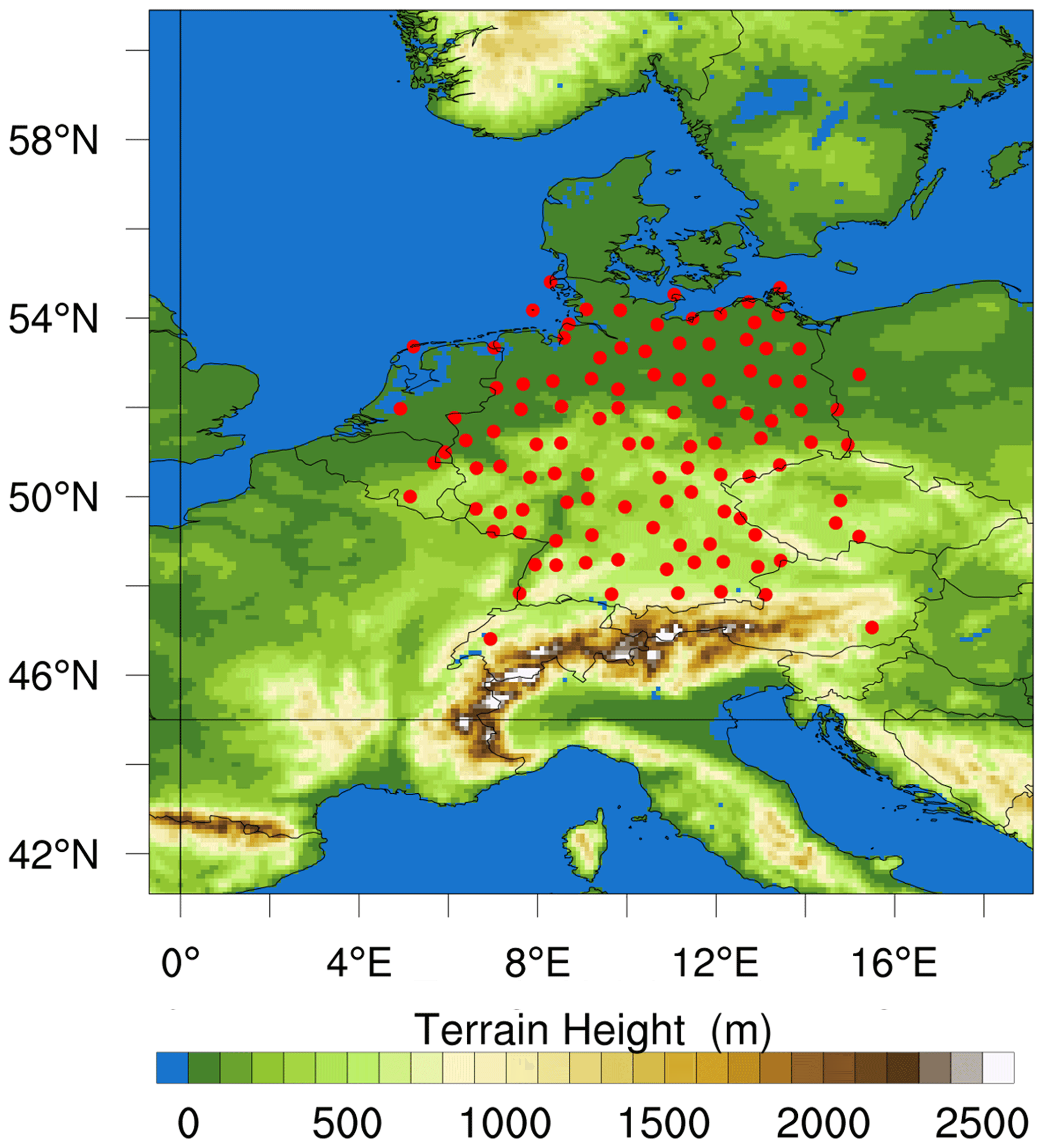
Figure 1The WRF model domain at a horizontal resolution of 0.1° (≈ 11 km) with the orography and the locations of GNSS stations.
For our model physics, we used the following parameters, as listed in Table 1. The radiation parameterization included the scheme of rapid radiative transfer model for general circulation models (RRTMG) (Iacono et al., 2008), which is known for accurately and efficiently calculating long-wave and short-wave fluxes and heating rates, particularly suited for general circulation model applications. The cloud microphysics scheme was the Thompson double-moment scheme (Thompson et al., 2008), capable of predicting mixing ratios for cloud water, rain, ice, snow, and graupel.
(Iacono et al., 2008)(Iacono et al., 2008)(Thompson et al., 2008)(Grell and Freitas, 2014)(Hong et al., 2010; Hong and Lim, 2006)(Chen and Dudhia, 2001)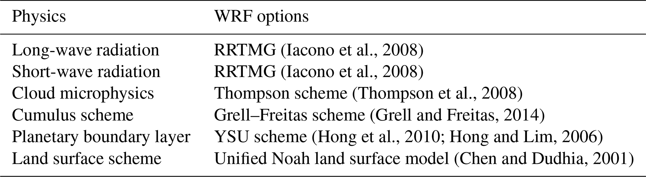
Our planetary boundary layer scheme of choice for this simulation was the Yonsei University (YSU) scheme (Hong et al., 2010; Hong and Lim, 2006). The YSU scheme, a non-local scheme with first-order closure, incorporates counter-gradient and explicit entrainment terms in the turbulence flux equation.
We utilized the unified Noah land surface model (Chen and Dudhia, 2001) for this study. This model comprises four layers and predicts soil temperature and moisture, canopy moisture, and snow cover. It considers various factors, including root zone dynamics, evapotranspiration, soil drainage, runoff variables, vegetation categories, and soil texture. This comprehensive approach provides valuable information on sensible and latent heat fluxes related to the boundary layer and incorporates an enhanced urban treatment.
To accurately simulate the model at a non-convective-scale resolution, it is essential to include convection parameterization. This helps represent the statistical impact of sub-grid-scale convective clouds. For this purpose, we employed the Grell–Freitas ensemble scheme (Grell and Freitas, 2014), which combines a probability density function with DA techniques.
3.2 Data assimilation system
The DA systems in WRF are typically classified into three categories: deterministic, probabilistic, and hybrid systems, which combine elements from both. In this study, we utilized the deterministic three-dimensional variational (3D-Var) DA system.
In the 3D-Var DA system, the objective is to iteratively minimize the cost function, J(x), where the independent or control variable is the analysis state vector, x. The cost function for the 3D-Var system is represented as follows:
The cost function, J(x), consists of two main terms: a background term and an observation term. The variables x, xb, and y are column vectors representing the analysis state, the background (or first guess), and the observation state, respectively. The forward operator, denoted as H, is responsible for mapping the analysis state vector space to the observation vector space. In this study, we have implemented the forward operator, H, specifically for GNSS tropospheric gradients.
Alongside the column vectors, there are two square matrices that play a crucial role in minimizing the cost function: the background error covariance matrix, B, and the observation error covariance matrix, R. R is a diagonal matrix because we assume that observation errors from various sources are uncorrelated. On the other hand, B is a square, positive semi-definite, and symmetric matrix with positive eigenvalues. It includes variances in background forecast errors in the diagonal and covariances between them on the symmetric upper and lower triangular elements. After assimilating an observation, the variances and covariances in B significantly influence the analysis response. Therefore, accurately determining B is essential in a variational DA system.
In this research, we computed the B matrix using the National Meteorological Center (NMC) method (Parrish and Derber, 1992). The NMC method is widely used for generating B by estimating climatological background error covariances. We selected the NMC method due to its ability to yield physically sound results within regional model domains and its lower computational cost compared to ensemble methods. The NMC method involves calculating forecast difference statistics to obtain the forecast error covariance tailored to a specific domain. However, it does have limitations, such as overestimating covariances in large-scale simulations and regions with poor observation (Berre, 2000; Fischer, 2013; Berre et al., 2006).
For our regional simulations, forecast statistics were derived from analyzing forecast differences over a month, utilizing both 24 and 12 h predictions. These statistics were obtained from data in June 2021. We chose the CV5 option as it allows independent control of moisture levels without interference from other variables. CV5 is a version of the background error covariance matrix used in WRF, which used five control variables such as stream function (Ψ), unbalanced velocity potential (χu), unbalanced temperature (Tu), pseudo-relative humidity (RHs), and unbalanced surface pressure (Ps,u). The pseudo-relative humidity is expressed as , where Qb,s represents the saturated specific humidity of the background field.
3.3 Experimental setup
The assimilation experiment was conducted for 2 months, in June and July 2021, using a rapid update cycle (RUC) approach, as illustrated in Fig. 2. The RUC was configured for 6-hourly DA cycles. The datasets employed for assimilation included: (1) conventional data, comprising surface stations (SYNOP), radiosondes, and Tropospheric Airborne Meteorological Data Reporting (TAMDAR) observations; (2) ZTDs; and (3) tropospheric gradients.

Figure 2Schematic of the 3D-Var rapid update cycle initialized from the GFS analysis. A spin-up of 12 h was performed until 00:00 UTC on 1 June 2021. Four experiments with different setups are performed: a control run (black) assimilating conventional data, a ZTD run (purple) assimilating ZTDs on top of the control run, a ZTDGRA run (red) assimilating ZTD and gradients on top of the control run, and a GRA run (green) assimilating gradients on top of the control run. The WRFDA namelist switch use_gpsgraobs has a value of 0 for ZTD assimilation and 1 for ZTD and gradient assimilation.
We performed four primary experiments for this study: (1) a control run, incorporating only conventional observations (SYNOP, radiosondes, and TAMDAR); (2) an impact run (ZTD run), assimilating ZTD observations in addition to the control run; (3) an impact gradient run (ZTDGRA run), where both ZTD and gradient observations were assimilated on top of the control run, using the newly developed gradient operator; and, finally, (4) a gradient run (GRA run), assimilating only gradients on top of the control run. The gradient-only assimilation was performed by down-weighting ZTDs by assigning a large observation error. The assimilation period spanned from 1 June 2021 at 00:00 UTC to 31 July 2021 at 18:00 UTC, with 6 h intervals, totaling 244 DA cycles. The initial DA cycle commenced after a 12 h spin-up run aiming to stabilize the model's initial and boundary conditions, ensuring reliable forecasts for subsequent DA.
3.4 Datasets for assimilation
3.4.1 Conventional datasets
To enhance the capabilities of the DA system, we established a comprehensive network of surface reports, SYNOP, across Europe. Radiosonde measurements, obtained through TEMP, provide a detailed view of the atmospheric thermodynamic structure at launch points. TEMP is a collection of alphanumerical codes established by the WMO. These codes represent upper-air soundings obtained through weather balloons launched from either land or sea level. These observations report on the weather conditions in the upper regions of the atmosphere. In WRFDA, FM-35 TEMP is the observation code used to identify radiosonde observations launched from land and FM-36 for those launched from ships. In order to compensate for the underrepresented radiosonde network during specific time periods, such as 06:00 and 18:00 UTC rather than 00:00 and 12:00 UTC, we utilized a series of TAMDAR observations. Table 2 summarizes the average number of observations assimilated per time step over 2 months. These valuable observations are conveniently accessible via the WMO's Global Telecommunication System data archive, which is housed at ECMWF.
Table 2Average number of observations assimilated per time step for June and July 2021.

To maintain simplicity within the DA system, we limited the use of conventional datasets to surface observations, radiosondes, and TAMDAR observations. It is worth noting that the primary objectives of this work are as follows: (1) to test the functionality of the newly developed operator (code) and (2) to analyze the difference between the experiment where we assimilate ZTDs only and the experiment where we assimilate both ZTDs and tropospheric gradients. In essence, our focus lies in assessing the relative impact rather than the absolute impact of GNSS data in variational DA.
3.4.2 GNSS ZTDs and tropospheric gradient observations
For detailed information regarding the GNSS analysis conducted at GFZ with its in-house software package EPOS (Earth Parameter and Orbit Determination System), readers are encouraged to refer to works such as Gendt et al. (2004).
For this research, we had around 380 GNSS stations provided by the GFZ that were distributed globally. In order to make a consistent set of observations within Germany, we removed the collocated and clustered stations. For this purpose, we selected only those GNSS stations whose data availability was above 75 %. As a result, we ended up with slightly more than 100 GNSS stations within Germany for the assimilation experiment.
To address potential biases in the GNSS dataset, we relied on analyses from our control experiment for bias correction. We utilized the 2-month simulation data from the control experiment to perform station-specific bias correction for GNSS ZTDs and gradient observations, which were then applied in the ZTD and ZTDGRA experiments. We assigned an observation error of 8 mm for the ZTD and 0.65 mm for the gradient for all observations. The observation error for the ZTD is motivated by previous assimilation studies. The choice of the observation error for the tropospheric gradient components is informed by an analysis of the observation-minus-background (OB) statistics from the control experiment (see “Results” below). It is important to note that the OB statistics represent a composite of observation and model errors, suggesting that our current choice for the observation error may be somewhat pessimistic. In future work, we plan to conduct sensitivity studies to obtain more accurate estimates for observation errors.
4.1 Single observation tests
To assess the impact of assimilating a single observation from a station location, we conducted the SOT in WRF. Through the SOT, our aim was to gain an insight into the model's behavior in response to GNSS gradient observations. The DA system employed here is the 3D-Var, where the extent of the assimilation impact largely depends on the B matrix. We sought answers to the following questions:
-
How does the impact region differ when compared to assimilating ZTD observations?
-
What distinguishes the SOTs resulting from the assimilation of gradients from those involving ZTD observations?
-
How sensitive is the model to the assimilation of a single gradient observation?
To address these questions, we selected a point at the center of the model domain and conducted SOTs with varying pseudo-ZTD and pseudo-gradient observations and their associated errors.
For questions 1 and 2, we conducted separate SOTs for gradients and ZTDs. In the gradient SOT, we selected an increment of −1.0 mm for the north gradient observation value and 0 mm for the east gradient observation value, with an observation error of 1.0 mm. In the ZTD SOT, we used an increment of 1.0 cm for the ZTD value and an observation error of 1.0 cm. We opted for unit values as errors to facilitate the understanding of the increment's impact without a scaling factor.
Figure 3 provides a comparison of the spatial impact resulting from SOTs using gradient and ZTD observations. This comparison helps us visualize how the impact spreads. The gradient impact plot in Fig. 3a justifies the name gradient as it reveals increased moisture in the south (positive lobe) and decreased moisture in the north (negative lobe), indicating a redistribution of moisture in the analysis. Visualizing the gradient increment as a vector pointing south aligns with the input values of −1.0 mm for the north gradient and 0 mm for the east gradient. Tropospheric gradients can be considered moisture vectors, similarly to wind vectors, encompassing both north–south and east–west components. Typically, tropospheric gradients point from dry to moist areas.
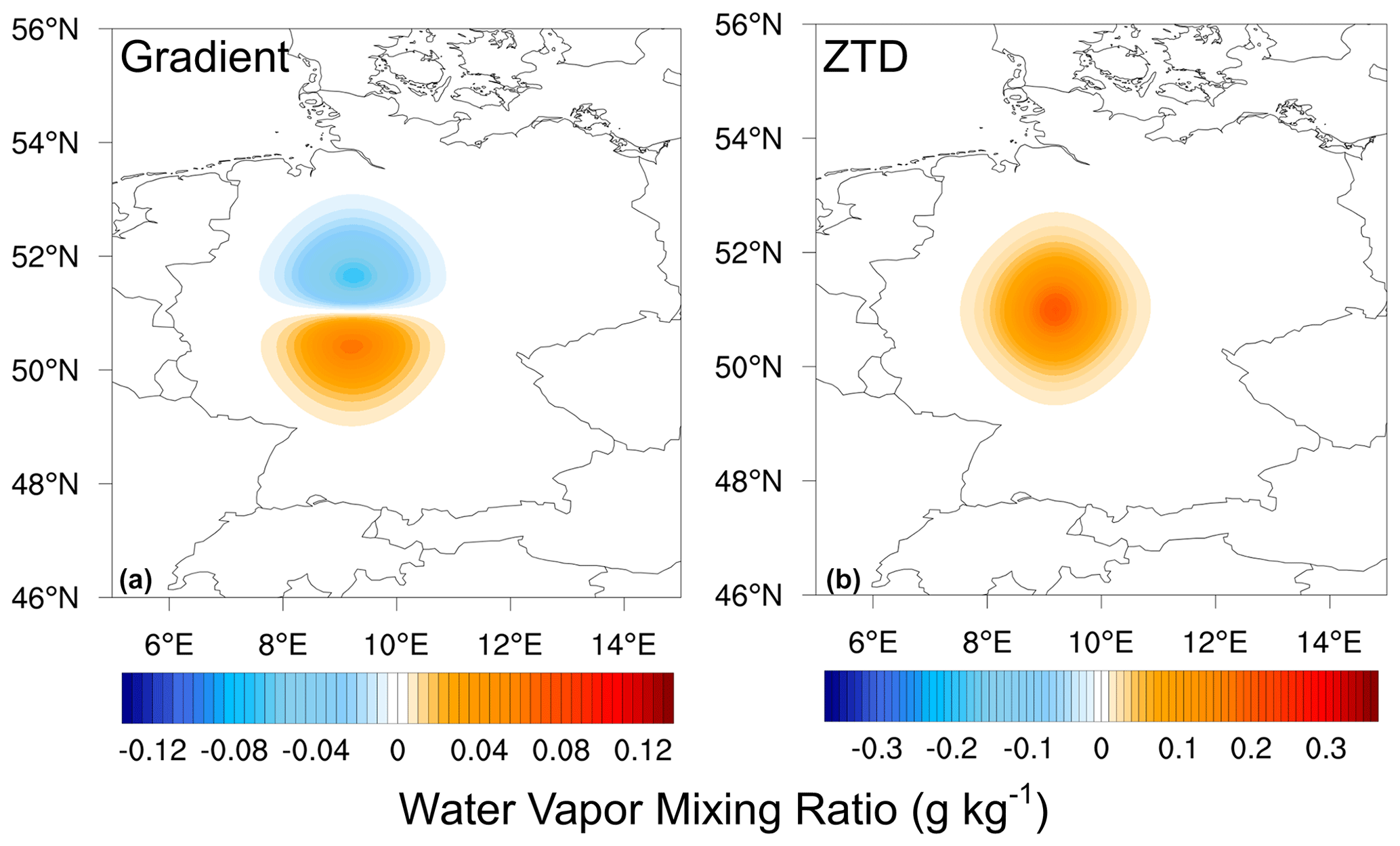
Figure 3Single observation test spatial plot of gradient and ZTD. An N gradient increment of −1.0 mm and an error of 1 mm are applied for the gradient SOT on the left. A ZTD increment of 1 cm and an error of 1 cm are applied on the right.
Comparing the spatial impact of SOTs, we observe that the maximum impact response for a −1 mm north gradient increment with a 1 mm error is 0.062 g kg−1. In contrast, the maximum response for the SOT due to a 1 cm magnitude ZTD increment with a 1 cm error is 0.2 g kg−1. The impact radius reduces by 50 % from 0.062 to 0.032 g kg−1 within a radius of 67 km for the gradient and around 80 km for the ZTD.
Figure 4 displays the water vapor mixing ratio (WVMR) and temperature profiles of the SOT analysis with respect to model levels. The profiles were drawn from the locations of the positive and negative lobes. In order to find out the locations of the lobes, the following steps were adopted:
-
We average the analysis over the vertical levels between 2 and 4 km, where the gradient observations have the maximum influence.
-
We determine the latitude and longitude of the point in the domain where the absolute value of the water vapor mixing ratio is maximum.
-
Through step 2, we get two maximum value points on both sides of the gradient observation location. The profile is derived from these two locations; hence, we get the lobes.
The gradient SOT profile exhibits both positive and negative lobes, explaining the positive and negative responses in the WVMR profile. The temperature response in both gradient and ZTD SOTs is negligible. It is evident that the impact, to a large extent, depends on the B matrix, particularly with the CV5 option, which assumes moisture independence from other variables.

Figure 4The vertical profile of the SOTs with the same settings as in Fig. 3. The gradient SOT on the left shows the positive and negative (dash) lobes of the impact.

The profile plots highlight that gradient observations have a more significant impact on the lower troposphere than on the surface level, where the impact is minimal. In contrast, ZTD impacts are more pronounced in the lower troposphere but significant at the surface level as well. A cross section in Fig. 5 further emphasizes this difference, showing that ZTD impact extends from the lower troposphere to the surface with only a slight decrease in the WVMR value compared to the gradient impact. The gradient impact is most prominent between 1 and 5.5 km, with minimal influence at the surface level.
To gain a more realistic understanding of the impact of tropospheric gradients, we conducted an SOT using an actual gradient observation from a GNSS station. We selected a station near the center of the model domain with the coordinates N and E. The observation values were 0.497 mm for the east gradient, 0.099 mm for the north gradient, with an observation error of 0.65 mm assigned. Unlike previous SOTs that focused on one gradient direction, this scenario involved increments in both the east and the north gradient components, resembling real scenarios. In this case, the gradient dipole's direction is the vector sum of the two gradient components. Figure 6 displays the spatial and profile plots of this SOT.
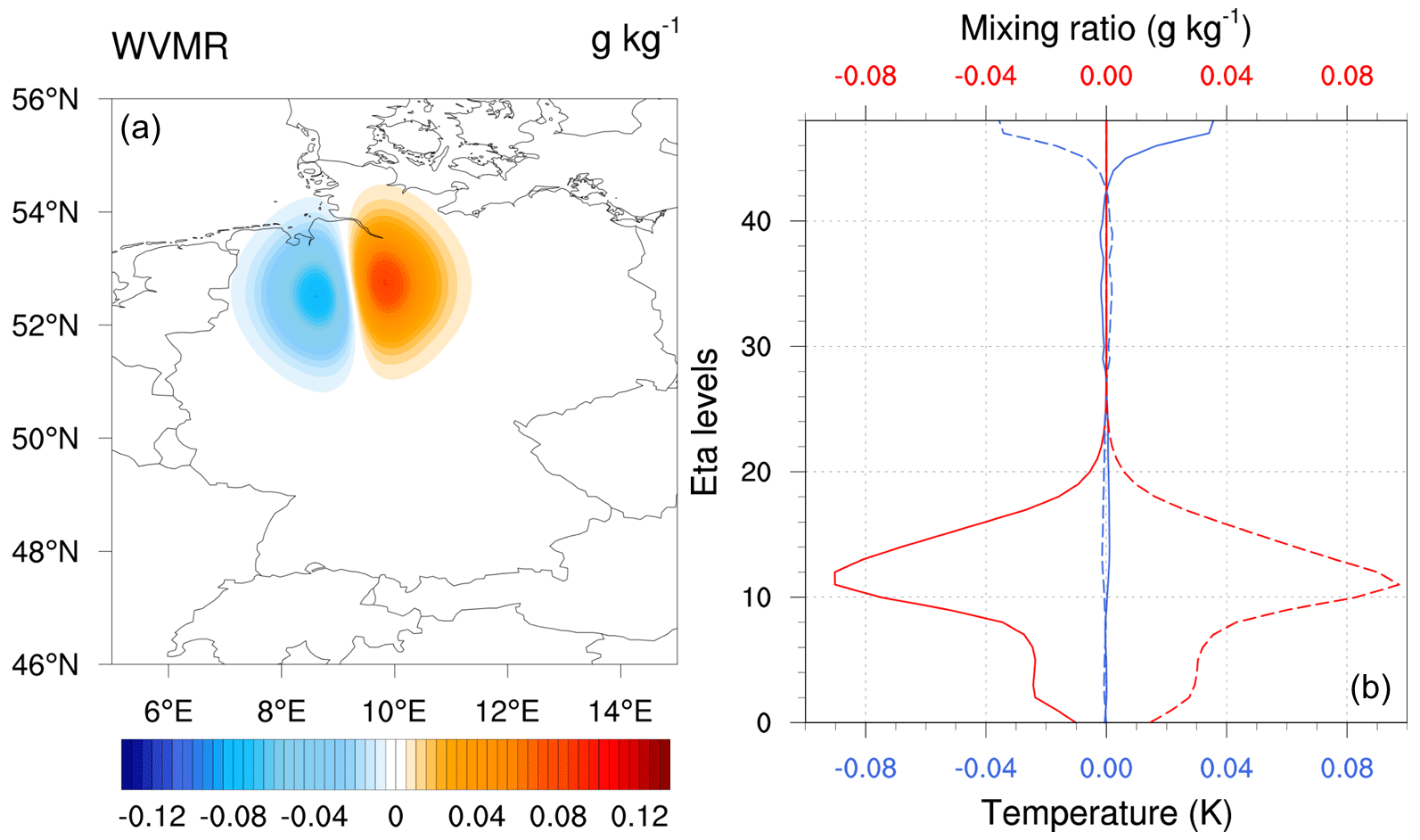
Figure 6A real observation SOT with gradient observations: the east gradient component equals 0.497 mm, and the north gradient component equals 0.099 mm. The observation error value for the SOT is chosen to be 0.65 mm, which is the standard error used for this study.
We modified the WRFDA code to allow users to conduct SOTs by adding specific options to the WRF namelist.input file.
4.2 Qualitative analysis of the gradient assimilation impact
This section aims to assess the noticeable impact of gradient observations on assimilation, specifically analyzing the spatio-temporal features emerging in the model as a result of assimilating gradients. To illustrate the influence of gradients, we compared the analyses obtained from the ZTDGRA and ZTD experiments using difference plots. The analysis is averaged over vertical levels between 2 and 4 km to capture the comprehensive impact from the lower troposphere, where gradient observations have the most significant influence.
Assimilation was conducted every 6 h in a RUC DA environment. In a RUC DA environment, the initial assimilation impact is of utmost importance as it reflects the analysis increment resulting from the assimilation of fresh observations, localized to their respective locations. As the cycles progress, the features tend to expand on a larger scale, making visual analysis more challenging. Therefore, our focus is primarily on the first and second DA cycles.
The initial DA cycle occurred on 1 June 2021, at 00:00 UTC. Following this, a 6 h free forecast was initiated based on the analysis until the next assimilation at 06:00 UTC. Figure 7 illustrates the initial DA cycle, with Fig. 7a showing the analysis difference observed at 00:00 UTC, while Fig. 7b–f display the forecast differences from 01:00 to 05:00 UTC. By comparing Fig. 7a with the station network in Fig. 1, it is evident that data from GNSS receivers in the region have had a substantial impact. Approximately 100 stations located exclusively in Germany have contributed to this impact. The absolute magnitude of the impact ranges from −0.15 to 0.14 g kg−1.
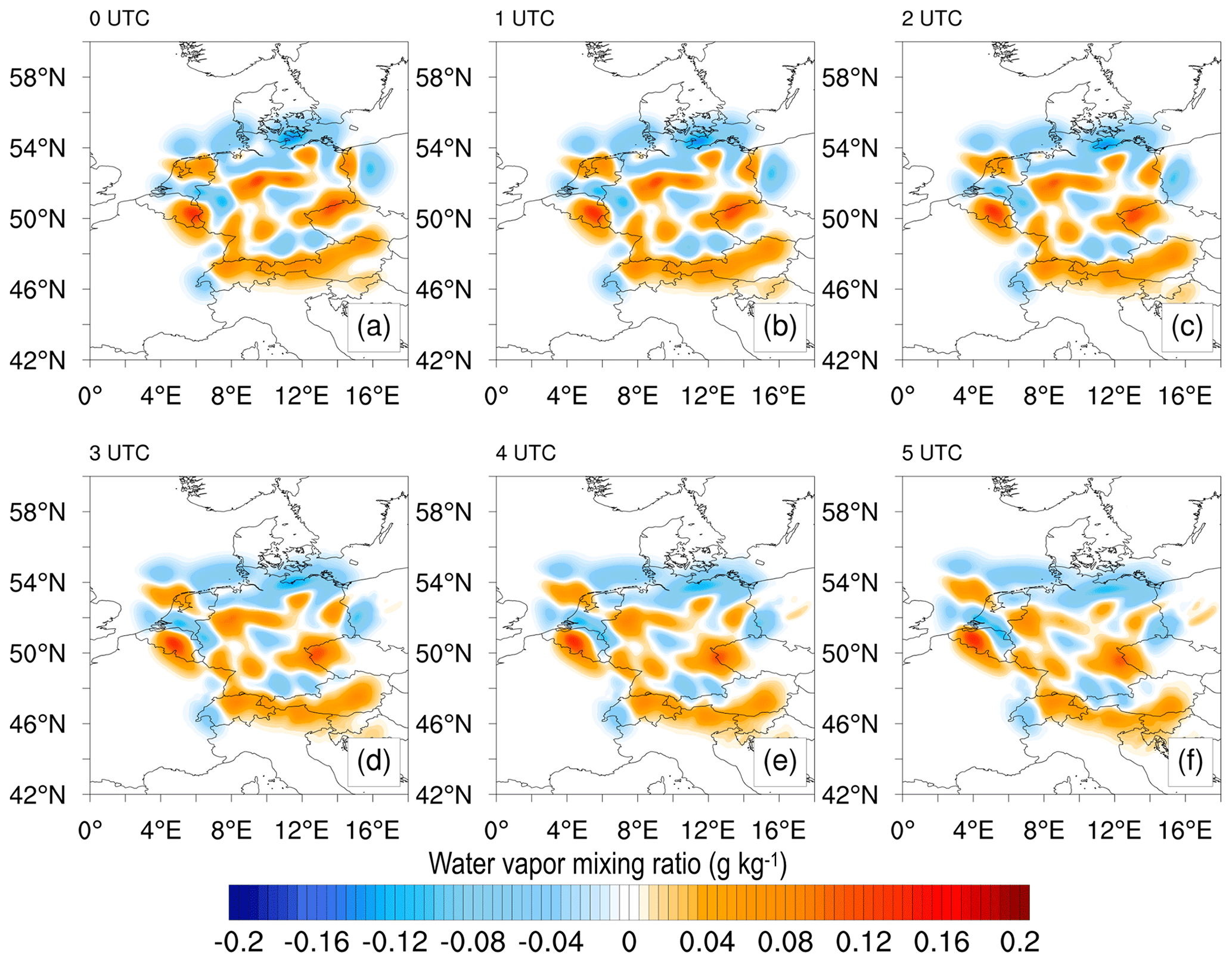
Figure 7Spatial analysis and forecast differences: ZTDGRA minus the ZTD experiment. The figure shows the exclusive impact of the gradient observation for the first DA cycle at 00:00 UTC (analysis) and the 5 h forecast from the analysis.
While the impact of assimilating gradients may seem relatively small in magnitude, it significantly affects the distribution of the moisture field in the initial model state (Fig. 7a). While these figures provide valuable insight, a quantitative analysis is necessary to determine if the assimilations have successfully corrected the model's moisture fields. Subsequent sections will delve into this topic, providing detailed comparisons for clarity.
Intercomparing Fig. 7b–f reveals that the impact of the gradients persists in the model for a significant period (6 h; until the next assimilation). This persistent impact serves as compelling evidence of the reliability of gradient data. Figure 8 reinforces this statement by displaying the analysis of the second DA cycle and the subsequent 6 h forecast difference. The structures developed during the forecast difference at 05:00 UTC are comparable to those observed in the analysis difference at 06:00 UTC during the second assimilation, as demonstrated by the comparison of Fig. 7f with Fig. 8a. The structures that emerged during the second assimilation were not significantly different from the forecast made before the assimilation, indicating that the gradient observations were accurate and that the assimilation did not degrade the model state nor did it tamper with the flow of the moisture fields.
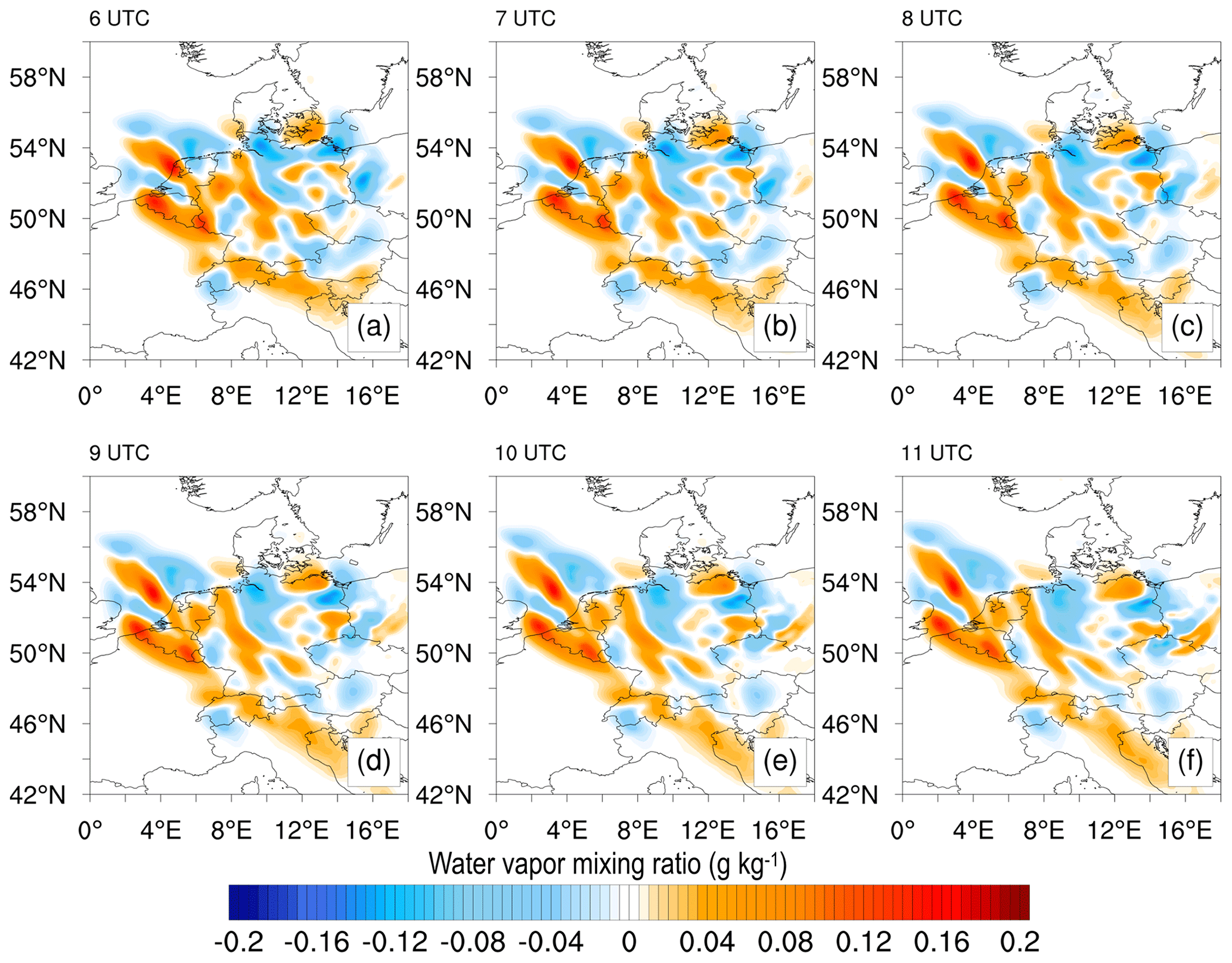
Figure 8Same as Fig. 7 but for the second DA cycle.
4.3 Quantitative analysis of the gradient assimilation impact
To comprehensively assess the impact of assimilating GNSS observations, we conducted a quantitative analysis and compared the results with the original station data from the GNSS network. Our objective was to gauge the extent of improvement achieved through this assimilation process. Our observation network initially comprised just over 100 GNSS stations. However, for validation purposes, we deliberately excluded 18 stations, categorizing them as “excluded” stations.
These excluded stations were strategically selected to ensure a balanced spatial distribution, aligning them with the locations of the German Weather Service (DWD) radar stations. They were set aside solely for independent validation purposes. The data from the remaining GNSS stations, known as the allowed stations, were assimilated in the ZTD, GRA, and ZTDGRA experiments. Consequently, we could evaluate the progress by comparing the assimilated data with the independent observations from these allowed stations.
This approach allowed us to rigorously assess the impact of our assimilation efforts and validate the improvements achieved. We will go through the Root Mean Square Error (RMSE) impact with respect to the allowed and excluded stations and also look into the average impact (in terms of RMSE) as a function of the forecast length in between the assimilation intervals.
4.3.1 RMSE with respect to allowed stations
To assess the impact of assimilating ZTD and gradient observations on the analyses in observation space, we computed the RMSE for four experiments: (1) control, (2) ZTD, (3) ZTDGRA, and (4) GRA using data from the allowed GNSS stations. We compared the ZTD and gradient values derived from the analyses at the station coordinates with the observations collected by GNSS stations. This comparison was performed over the entire 2-month period, using hourly data and considering all allowed stations. Figure 9 presents the station-specific RMSEs for the control, ZTD, ZTDGRA, and GRA experiments. The mean RMSE is listed in Table 3.
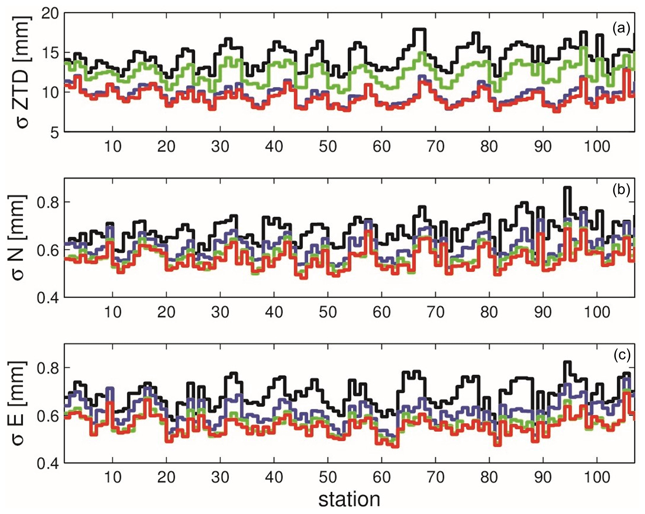
Figure 9The station-specific RMSE of the ZTD, north and east components (allowed stations): control (black), GRA (green), ZTD (purple), and ZTDGRA (red).
Table 3Comparison of the mean μ in mm of station-specific RMSE of ZTDs and gradients (W for allowed and B for excluded stations).
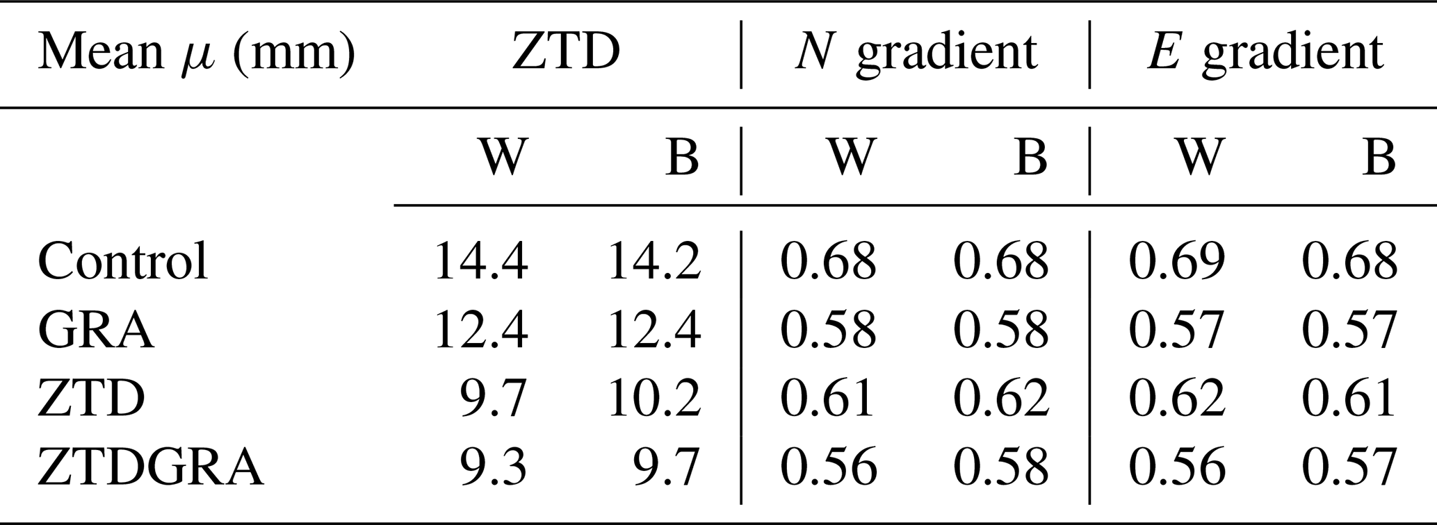
From the figure, it is evident that when assessing the improvement in the ZTD variable, the mean RMSE values for the ZTD parameter are the lowest for the ZTDGRA experiment compared to the other runs, providing clear evidence of the successful gradient assimilation impact. The mean RMSE of the ZTD variable for the control run was 14.4 mm, which was reduced to 9.7 mm in the ZTD run and further decreased to 9.3 mm in the ZTDGRA run. The GRA experiment also had an impact on the ZTD analysis. The GRA RMSE of 12.2 mm was in between that of the control and the ZTD experiments.
Regarding the impact on gradient components, both the north and east components exhibit similar enhancements. Notably, the ZTDGRA assimilation leads to the most significant improvement when compared to the other runs. The north (east) gradient RMSE decreased from 0.68 mm (0.69 mm) in the control run to 0.61 mm (0.62 mm) in the ZTD run and further decreased to 0.56 mm (0.56 mm) in the ZTDGRA run. From the GRA experiment, the impact of gradients was clearly evident. There was a significant reduction in RMSE from 0.68 mm (0.69 mm) in the control to 0.58 mm (0.57 mm) in the GRA for the north (east) gradients. The results are almost equal to those of the ZTDGRA run. The assimilation of gradients significantly reduced the RMSE values, indicating a substantial enhancement of the moisture field in the model state.
The results shown in Fig. 9 can be interpreted as follows: when assimilating only ZTDs, not only are the ZTDs adjusted, but the tropospheric gradients are also affected. Also, the assimilation of the gradients alone improves not only gradient analyses, but also the ZTDs. This suggests that tropospheric gradients contain valuable information. Such adjustment would not be possible if tropospheric gradients contained no useful data. However, as long as we do not assimilate tropospheric gradients, we do not make use of their information. This is addressed in the experiment, where both the ZTDs and the tropospheric gradients are assimilated. It can be observed that the tropospheric gradients are further adjusted, demonstrating the functionality of our implementation and that the ZTDs are also further adjusted, providing evidence that we extracted valuable information from the tropospheric gradients. Also, through the GRA run, it is clear that ZTDs do not provide weightage to improve the gradients. However, the ZTD plays a role in improving the gradient and vice versa.
4.3.2 RMSE with respect to excluded stations
To further evaluate the consistency of our findings from the allowed stations, we conducted a similar analysis using the 18 excluded stations. We measured the RMSE values as described previously but specifically for these 18 stations. This comparison was performed using hourly data over the entire 2-month period to provide a robust statistical assessment. Figure 10 presents the RMSE comparisons for the control, ZTD, ZTDGRA, and GRA experiments, using data from the excluded stations.

Figure 10The station specific RMSE of the ZTD, north and east components (excluded stations): control (black), GRA (green), ZTD (purple), and ZTDGRA (red).
In the figure, it is evident that the RMSE values for the ZTD variable have decreased. The mean RMSE for the ZTD variable decreased from 14.2 mm in the control run to 10.2 mm in the ZTD run and was further reduced to 9.7 mm in the ZTDGRA run. The GRA run also contributed to a reduction in RMSE from 14.2 mm in the control to 12.2 mm. Table 3 lists the mean RMSE for all the runs.
Similar improvements in the north and east gradient components were observed, mirroring the results obtained with the allowed stations. The RMSE values for the north (east) gradient component dropped from 0.68 mm (0.68 mm) in the control run to 0.62 mm (0.61 mm) in the ZTD run and further decreased to 0.58 mm (0.57 mm) in the ZTDGRA run. In the GRA experiment, it was observed that gradients had a clear impact, similarly to the comparisons of allowed stations. There was a significant decrease in RMSE from 0.68 mm in the control to 0.58 mm in the north and 0.57 mm in the east gradients. These results were nearly equivalent to those of the ZTDGRA run.
These results clearly demonstrate that the assimilation of gradients has enhanced the model's analyses. The 2-month statistics using independent GNSS station data validate the improvements achieved through gradient assimilation.
4.3.3 Average impact as a function of forecast length
As our assimilation process occurs every 6 h, we inherently have a 6 h forecast lead time. To calculate the mean RMSE for both ZTD and gradients, while considering both allowed and excluded stations, we examined the mean RMSE values across forecast lead times ranging from 0 to 5 h, similarly to our previous analysis. Figure 11 illustrates the RMSE variation with respect to forecast length.

Figure 11Average impact with respect to forecast lead times from analyses for 2 months of simulation. The control run (black), GRA run (green), ZTD run (purple), and ZTDGRA run (red) are shown for the allowed stations (a, b, c) and for the excluded stations (d, e, f).
In both allowed and excluded stations, the ZTDGRA experiment consistently outperforms the other runs, displaying the lowest RMSE values. As expected, the RMSE tends to increase as the lead time extends. However, what is noteworthy is the sustained improvement in RMSE across different forecast lead times in both allowed and excluded stations. This consistency of the improvement provides further evidence of the positive impact of gradients on the model state's moisture field. It is more evident in the GRA run, where the gradient forecast RMSE outperforms the ZTD. This is a clear sign that there is no weightage from the ZTD observations for improving the gradients. Additionally, the ZTDGRA experiment maintains a stable RMSE improvement throughout the forecast lead time, indicated by the small but consistent offset.
4.4 Comparison with ERA5
In addition to GNSS observation data, we conducted validation using the ERA5 dataset, which is considered one of the most comprehensive atmospheric reanalyses of the global climate to date, produced by the Copernicus Climate Change Service at ECMWF. ERA5 provides hourly estimates of climate variables globally on a 30 km grid, offering detailed atmospheric information with 137 levels up to 80 km in altitude. Given its high quality, ERA5 serves as a valuable reference dataset. To perform this validation, we selected five locations within the model domain, as shown in Fig. 12. With a total of 244 assimilation cycles, each generating five profiles, we had a substantial dataset of 1220 profiles for comparison with ERA5. This large number of profiles allowed us to obtain robust statistical results.

Figure 12ERA5 comparison domain. The station map and the selected points for the comparison of the ERA5 data with the analyses.
We compared the water vapor (WV) profiles for three different lead times after the assimilation cycles: 0, 3, and 5 h. Figure 13 presents the WV 1-sigma deviation between the assimilation experiments and ERA5 as a function of altitude for these three lead times. The findings from Fig. 13 indicate that assimilating ZTDs has a positive impact across the entire altitude range. This confirms that the assimilation of ZTDs results in an improvement in the WV field.
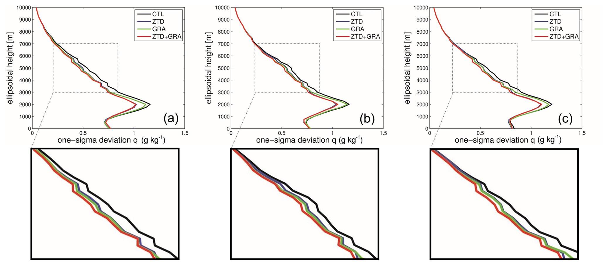
Figure 13ERA5 profile comparison. The statistics of 1220 profiles for the control run (black), GRA (green), ZTD run (purple), and ZTDGRA run (red) are shown for the analyses (00:00 UTC) in the leftmost column, 3 h time lead in the middle column, and 5 h time lead in the rightmost column. The bottom row shows the magnified lower-troposphere profiles.
Furthermore, the assimilation of tropospheric gradients, in addition to ZTDs, leads to further improvements in the WV field. However, it is important to note that this improvement is primarily restricted to altitudes above 2.5 km. Below an altitude of 2.5 km, particularly near the Earth's surface, the assimilation of gradients, in addition to ZTDs, does not have a significant impact. This lack of impact close to the Earth's surface is not surprising, as gradients are not sensitive to surface variables (as indicated by Eqs. 4 and 5). Any impact near the surface can be attributed to the background error covariance matrix and its correlations between different altitudes, as observed in the SOT experiment. It is possible to gain more insight into the impact of observations by differentiating the ZTD and GRA profiles. GRA has more influence on the lower troposphere but not on the surface, whereas the ZTD has a greater impact on the surface level.
The positive impact of gradient assimilation remains consistent across different lead times. In essence, the reduction in the standard deviation above 2.5 km observed in the ZTDGRA experiment remains consistent even at the 5 h lead time.
4.5 Forecast comparison with radiosonde profiles
Forecast validation was carried out for the analysis forecasts generated in all four experiments. The analyses valid at 00:00 UTC from each of these experiments were subjected to a free forecast of 12 h in length. The 12 h forecasts were prepared starting from the DA cycle at 00:00 UTC on 1 June 2021, and continuing until 00:00 UTC on 30 July 2021. Figure 14 shows the average RMSE of the mixing ratio up through the radiosonde profile for 60 d. Since radiosonde profiles are usually available at irregular heights, we interpolated the model profiles to those of the radiosondes. Hence, the model profiles of the 12 h forecast from the analyses were compared with the radiosonde profiles at that time instant to calculate the RMSE. We compared the forecasts valid at 12:00 UTC (forecasted from analyses at 00:00 UTC) with the radiosondes at 12:00 UTC, since there were more radiosondes during that time, to get the statistics. There were a minimum of 38 radiosondes available for comparison.
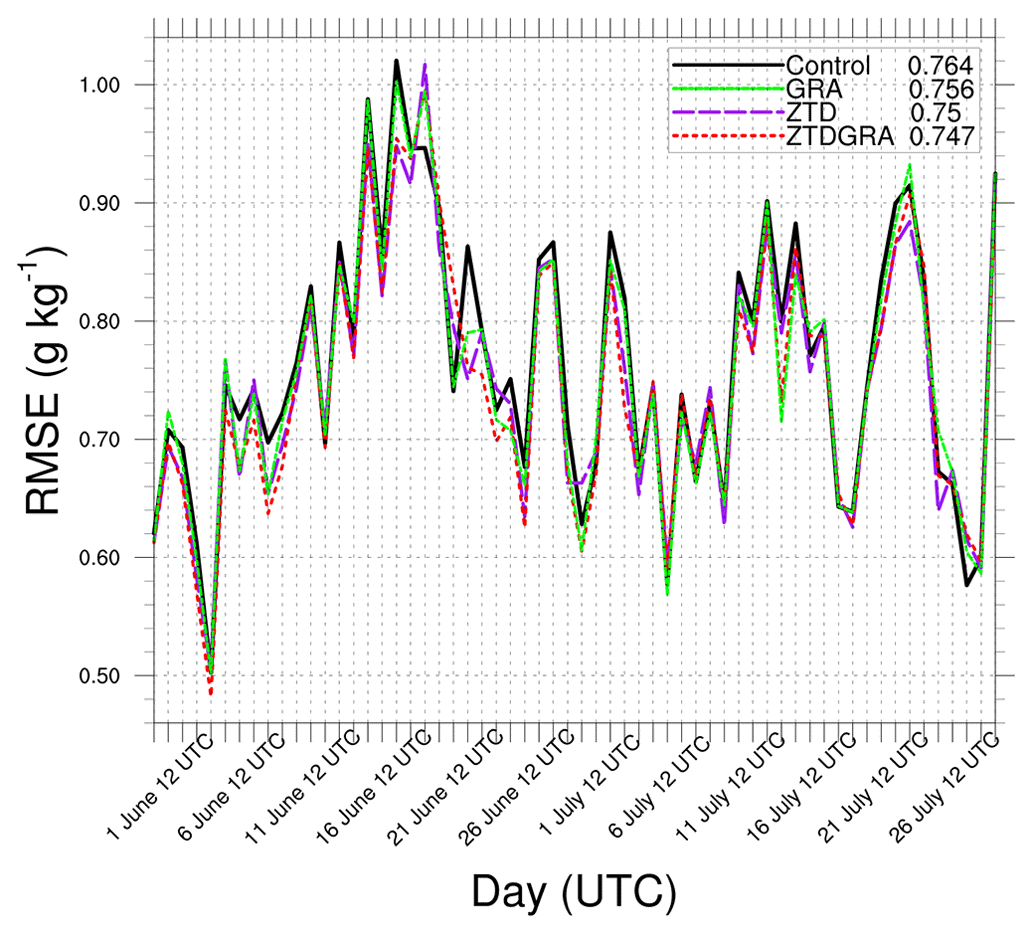
Figure 14Water vapor mixing ratio comparison of the 12 h forecasts from the analyses valid at 00:00 UTC to the radiosonde profiles at 12:00 UTC (around 38 radiosondes per epoch). The mean RMSEs (g kg−1) of the respective runs for the 2 months are specified in the legend.
While the improvement observed in the ZTDGRA experiment is notable, it remains relatively modest. It is important to note that this improvement may not persist beyond the 12th hour of forecasting. Additionally, any non-uniformity among the radiosonde profiles could potentially impact the final assessment of these improvements. However, from the mean RMSE, we understand that incorporating the gradient observations improves the forecasts. The mean RMSEs in descending order are control, GRA, ZTD, and, finally, ZTDGRA.
In this study, we successfully implement a newly developed gradient observation operator within the WRFDA system, allowing us to assimilate GNSS tropospheric gradients. We utilize WRF version 4.4.1 along with the 3D-Var DA system, configuring the model to a resolution of 0.1° (≈ 11 km) and 50 vertical levels. Our dataset includes GNSS ZTDs and tropospheric gradient observations obtained from over 100 GNSS ground-based stations covering Germany. Assimilations were performed at 6 h intervals over a 2-month period in June and July 2021.
To assess the impact of tropospheric gradients, we conducted four distinct model simulations. The first was a control run, which incorporated only conventional observations. The second, the ZTD run, involved assimilating ZTDs in addition to conventional observations on top of the control run. The third, the ZTDGRA run, assimilated both ZTDs and gradients alongside conventional observations on top of the control run. Furthermore, the GRA run only assimilated gradients on top of the control run.
Our results clearly demonstrated the positive impact of tropospheric gradient observations when assimilated using the gradient operator. The ZTDGRA experiment exhibited the smallest RMSE (measured in observation space) compared to the other experiments, confirming that gradient observations contained valuable information and significantly improved the initial state of the model. The RMSE for the ZTD run was reduced by 32 % for ZTDs and 10 % for gradients, while the ZTDGRA run saw a reduction of 35 % for ZTDs and 18 % for gradients. The GRA run had a significant impact on the gradient analyses. The results were almost equal to that of the ZTDGRA for the gradients, and the improvement in the ZTDs was better than for the control run. Of course, the GRA run not only illustrated the exclusive impact of the gradients where the assimilation improved the gradients, but also slightly improved the ZTDs. Also, the vice versa is true; ZTD plays a role in improving the gradient.
Additionally, our forecasts generated from the analyses exhibited improved accuracy when compared to ERA5 and radiosonde data, suggesting that the gradient information persisted in the model for at least 6 h. It is important to note that the most significant impact of gradient observations was observed in the lower troposphere, with negligible effects on the surface level.
In this research, we introduce the capability to incorporate a new observation type (i.e., tropospheric gradients), which has yet to be utilized by the operational forecast community or research groups. In the control run, we kept only the critical observation types, such as surface stations, radiosondes, and TAMDAR observations, to demonstrate how gradients impact the analyses. In the future, we plan to test the impact by incorporating observations like satellite radiances in the control run. However, we still expect a slight improvement if we add ZTDs and gradients on top of the conventional observations. As a pioneering research using GNSS gradients, the first step in this article is to assimilate gradient observations through an observation operator. While our study focused on the relative impact of gradient assimilation, we acknowledge that further improvements can be achieved through ensemble-based DA systems. Ensemble DA systems utilize flow-dependent background error covariance matrices, considering the dynamic nature of the atmosphere, and are expected to provide a more accurate representation of humidity variables in real-time scenarios. Quantifying the improvement made by gradients in predicting severe weather for operational purposes, as mentioned in EGMAP, is a topic for another article with an ensemble-based DA system.
We want to share the GNSS gradient operator with the GNSS meteorological community to optimize gradients and determine ways of using this abundant observation type in the operational forecast centers worldwide. We hope the readers can test the operator and make some improvements to the existing version. With our source codes openly available, we encourage fellow researchers to conduct their own GNSS DA experiments assimilating gradient data and further build upon our findings to advance the field of atmospheric modeling and forecasting.
The complete WRFDA code version 4.4.1, with the gradient operator codes and the simulation experiment data and including the namelist files and data used for all assimilation cycles, is available for download. The experiment data include a 6-hourly analysis for the three experiments – control, ZTD, and ZTDGRA – for June and July 2021. All files are stored on Zenodo, a general-purpose open repository developed under the European Open-Access Infrastructure for Research in Europe (OpenAIRE) program and operated by the European Organization for Nuclear Research (CERN). The access link is https://doi.org/10.5281/zenodo.10276429 (Thundathil, 2023).
The original draft of the study was written by RT, who also conducted the formal analysis and experiments. FZ and RT collaborated to modify the WRFDA code and develop the gradient operator. JW and GD supervised the project, acquired funding, and reviewed and edited the paper.
The contact author has declared that none of the authors has any competing interests.
Publisher's note: Copernicus Publications remains neutral with regard to jurisdictional claims made in the text, published maps, institutional affiliations, or any other geographical representation in this paper. While Copernicus Publications makes every effort to include appropriate place names, the final responsibility lies with the authors.
The research project is funded by the German Research Foundation (DFG; grant no. 68510200) and titled “Exploitation of GNSS tropospheric gradients for severe weather Monitoring And Prediction (EGMAP)”. The ECMWF conventional datasets for the DA study in this research were provided by Thomas Schwitalla from our collaborative institution, Institute of Physics and Meteorology, University of Hohenheim, Stuttgart. Zenodo (https://zenodo.org/, last access: 30 April 2024) is used to store the model code and simulation data.
This research has been supported by the German Research Foundation (grant no. 68510200).
This open-access publication was funded by Technische Universität Berlin.
This paper was edited by Nina Crnivec and reviewed by two anonymous referees.
Bar-Sever, Y. E., Kroger, P. M., and Borjesson, J. A.: Estimating horizontal gradients of tropospheric path delay with a single GPS receiver, J. Geophys. Res.-Sol. Ea., 103, 5019–5035, 1998. a, b
Bennitt, G. V. and Jupp, A.: Operational assimilation of GPS zenith total delay observations into the Met Office numerical weather prediction models, Mon. Weather Rev., 140, 2706–2719, 2012. a
Berre, L.: Estimation of synoptic and mesoscale forecast error covariances in a limited-area model, Mon. Weather Rev., 128, 644–667, 2000. a
Berre, L., Ştefaănescu, S. E., and Pereira, M. B.: The representation of the analysis effect in three error simulation techniques, Tellus A, 58, 196–209, 2006. a
Bevis, M., Businger, S., Herring, T. A., Rocken, C., Anthes, R. A., and Ware, R. H.: GPS meteorology: Remote sensing of atmospheric water vapor using the global positioning system, J. Geophys. Res.-Atmos., 97, 15787–15801, 1992. a
Boniface, K., Ducrocq, V., Jaubert, G., Yan, X., Brousseau, P., Masson, F., Champollion, C., Chéry, J., and Doerflinger, E.: Impact of high-resolution data assimilation of GPS zenith delay on Mediterranean heavy rainfall forecasting, Ann. Geophys., 27, 2739–2753, https://doi.org/10.5194/angeo-27-2739-2009, 2009. a
Brenot, H., Neméghaire, J., Delobbe, L., Clerbaux, N., De Meutter, P., Deckmyn, A., Delcloo, A., Frappez, L., and Van Roozendael, M.: Preliminary signs of the initiation of deep convection by GNSS, Atmos. Chem. Phys., 13, 5425–5449, https://doi.org/10.5194/acp-13-5425-2013, 2013. a
Caldas-Alvarez, A. and Khodayar, S.: Assessing atmospheric moisture effects on heavy precipitation during HyMeX IOP16 using GPS nudging and dynamical downscaling, Nat. Hazards Earth Syst. Sci., 20, 2753–2776, https://doi.org/10.5194/nhess-20-2753-2020, 2020. a
Chen, F. and Dudhia, J.: Coupling an advanced land surface–hydrology model with the Penn State–NCAR MM5 modeling system. Part I: Model implementation and sensitivity, Mon. Weather Rev., 129, 569–585, 2001. a, b
Chen, S.-Y., Huang, C.-Y., Kuo, Y.-H., Guo, Y.-R., and Sokolovskiy, S.: Assimilation of GPS refractivity from FORMOSAT-3/COSMIC using a nonlocal operator with WRF 3DVAR and its impact on the prediction of a typhoon event, Terr. Atmos. Ocean. Sci., 20, 133–154, https://doi.org/10.3319/TAO.2007.11.29.01(F3C), 2009. a
Davis, J. L., Elgered, G., Niell, A. E., and Kuehn, C. E.: Ground-based measurement of gradients in the “wet” radio refractivity of air, Radio Sci., 28, 1003–1018, 1993. a
Douša, J., Dick, G., Kačmařík, M., Brožková, R., Zus, F., Brenot, H., Stoycheva, A., Möller, G., and Kaplon, J.: Benchmark campaign and case study episode in central Europe for development and assessment of advanced GNSS tropospheric models and products, Atmos. Meas. Tech., 9, 2989–3008, https://doi.org/10.5194/amt-9-2989-2016, 2016. a
Dousa, J., Vaclavovic, P., and Elias, M.: Tropospheric products of the second GOP European GNSS reprocessing (1996–2014), Atmos. Meas. Tech., 10, 3589–3607, https://doi.org/10.5194/amt-10-3589-2017, 2017. a
Fischer, L.: Statistical characterisation of water vapour variability in the troposphere, Ph.D. thesis, LMU München, Faculty of Physics, https://doi.org/10.5282/edoc.16208, 2013. a
Gendt, G., Dick, G., Reigber, C., Tomassini, M., Liu, Y., and Ramatschi, M.: Near real time GPS water vapor monitoring for numerical weather prediction in Germany, J. Meteor. Soc. Jpn. Ser. II, 82, 361–370, 2004. a, b
Giannaros, C., Kotroni, V., Lagouvardos, K., Giannaros, T. M., and Pikridas, C.: Assessing the impact of GNSS ZTD data assimilation into the WRF modeling system during high-impact rainfall events over Greece, Remote Sens., 12, 383, https://doi.org/10.3390/rs12030383, 2020. a
Giering, R. and Kaminski, T.: Recipes for adjoint code construction, ACM T. Mathe. Softw., 24, 437–474, 1998. a
Grell, G. A. and Freitas, S. R.: A scale and aerosol aware stochastic convective parameterization for weather and air quality modeling, Atmos. Chem. Phys., 14, 5233–5250, https://doi.org/10.5194/acp-14-5233-2014, 2014. a, b
Hong, S.-Y. and Lim, J.-O. J.: The WRF single-moment 6-class microphysics scheme (WSM6), Asia-Pac. J. Atmos. Sci., 42, 129–151, 2006. a, b
Hong, S.-Y., Lim, K.-S. S., Lee, Y.-H., Ha, J.-C., Kim, H.-W., Ham, S.-J., and Dudhia, J.: Evaluation of the WRF double-moment 6-class microphysics scheme for precipitating convection, Adv. Meteorol., 2010, 707253, https://doi.org/10.1155/2010/707253., 2010. a, b
Iacono, M. J., Delamere, J. S., Mlawer, E. J., Shephard, M. W., Clough, S. A., and Collins, W. D.: Radiative forcing by long-lived greenhouse gases: Calculations with the AER radiative transfer models, J. Geophys. Res.-Atmos., 113, D13103, https://doi.org/10.1029/2008JD009944, 2008. a, b, c
Iwabuchi, T., Miyazaki, S., Heki, K., Naito, I., and Hatanaka, Y.: An impact of estimating tropospheric delay gradients on tropospheric delay estimations in the summer using the Japanese nationwide GPS array, J. Geophys. Res.-Atmos., 108, 4315, https://doi.org/10.1029/2002JD002214, 2003. a
Kačmařík, M., Douša, J., Zus, F., Václavovic, P., Balidakis, K., Dick, G., and Wickert, J.: Sensitivity of GNSS tropospheric gradients to processing options, Ann. Geophys., 37, 429–446, https://doi.org/10.5194/angeo-37-429-2019, 2019. a
Lagasio, M., Parodi, A., Pulvirenti, L., Meroni, A. N., Boni, G., Pierdicca, N., Marzano, F. S., Luini, L., Venuti, G., Realini, E., Gatti, A., Tagliaferro, G., Barindelli, S., Monti Guarnieri, A., Goga, K., Terzo, O., Rucci, A., Passera, E., Kranzlmueller, D., and Rommen, B.: A synergistic use of a high-resolution numerical weather prediction model and high-resolution earth observation products to improve precipitation forecast, Remote Sens., 11, 2387, https://doi.org/10.3390/rs11202387, 2019. a
Li, X., Dick, G., Lu, C., Ge, M., Nilsson, T., Ning, T., Wickert, J., and Schuh, H.: Multi-GNSS meteorology: real-time retrieving of atmospheric water vapor from BeiDou, Galileo, GLONASS, and GPS observations, IEEE T. Geosci. Remote, 53, 6385–6393, 2015. a
Lindskog, M., Ridal, M., Thorsteinsson, S., and Ning, T.: Data assimilation of GNSS zenith total delays from a Nordic processing centre, Atmos. Chem. Phys., 17, 13983–13998, https://doi.org/10.5194/acp-17-13983-2017, 2017. a
Mahfouf, J.-F., Ahmed, F., Moll, P., and Teferle, F. N.: Assimilation of zenith total delays in the AROME France convective scale model: a recent assessment, Tellus A, 67, 26106, https://doi.org/10.3402/tellusa.v67.26106, 2015. a
Mascitelli, A., Federico, S., Fortunato, M., Avolio, E., Torcasio, R. C., Realini, E., Mazzoni, A., Transerici, C., Crespi, M., and Dietrich, S.: Data assimilation of GPS-ZTD into the RAMS model through 3D-Var: preliminary results at the regional scale, Meas. Sci. Technol., 30, 055801, https://doi.org/10.1088/1361-6501/ab0b87, 2019. a
Mascitelli, A., Federico, S., Torcasio, R., and Dietrich, S.: Assimilation of GPS Zenith Total Delay estimates in RAMS NWP model: Impact studies over central Italy, Adv. Space Res., 68, 4783–4793, 2021. a
Morel, L., Pottiaux, E., Durand, F., Fund, F., Boniface, K., de Oliveira Junior, P. S., and Van Baelen, J.: Validity and behaviour of tropospheric gradients estimated by GPS in Corsica, Adv. Space Res., 55, 135–149, 2015. a
Parrish, D. F. and Derber, J. C.: The National Meteorological Center's spectral statistical-interpolation analysis system, Mon. Weather Rev., 120, 1747–1763, 1992. a
Poli, P., Moll, P., Rabier, F., Desroziers, G., Chapnik, B., Berre, L., Healy, S., Andersson, E., and El Guelai, F.-Z.: Forecast impact studies of zenith total delay data from European near real-time GPS stations in Météo France 4DVAR, J. Geophys. Res.-Atmos., 112, D06114, https://doi.org/10.1029/2006JD007430, 2007. a
Rohm, W., Guzikowski, J., Wilgan, K., and Kryza, M.: 4DVAR assimilation of GNSS zenith path delays and precipitable water into a numerical weather prediction model WRF, Atmos. Meas. Tech., 12, 345–361, https://doi.org/10.5194/amt-12-345-2019, 2019. a
Skamarock, W. C., Klemp, J. B., Dudhia, J., Gill, D. O., Barker, D. M., Duda, M. G., Huang, X.-Y., Wang, W., and Powers, J. G.: A description of the advanced research WRF version 3, NCAR technical note, 475, 113, https://doi.org/10.5065/D68S4MVH, 2008. a
Thayer, G. D.: An improved equation for the radio refractive index of air, Radio Sci., 9, 803–807, 1974. a
Thompson, G., Field, P. R., Rasmussen, R. M., and Hall, W. D.: Explicit forecasts of winter precipitation using an improved bulk microphysics scheme. Part II: Implementation of a new snow parameterization, Mon. Weather Rev., 136, 5095–5115, 2008. a, b
Thundathil, R. M.: Assimilation of GNSS Tropospheric Gradients into the Weather Research and Forecasting Model Version 4.4.1, Zenodo [code], https://doi.org/10.5281/zenodo.10276429, 2023. a, b
Vedel, H. and Huang, X.-Y.: Impact of ground based GPS data on numerical weather prediction, J. Meteorol. Soc. Jpn. Ser. II, 82, 459–472, 2004. a
Walpersdorf, A., Calais, E., Haase, J., Eymard, L., Desbois, M., and Vedel, H.: Atmospheric gradients estimated by GPS compared to a high resolution numerical weather prediction (NWP) model, Phys. Chem. Earth, A, 26, 147–152, 2001. a
Wickert, J., Dick, G., Schmidt, T., Asgarimehr, M., Antonoglou, N., Arras, C., Brack, A., Ge, M., Kepkar, A., Männel, B., Nguyen, C., Oluwadare, T. S., Schuh, H., Semmling, M., Simeonov, T., Vey, S., Wilgan, K., and Zus, F.: GNSS remote sensing at GFZ: Overview and recent results, ZfV-Zeitschrift für Geodäsie, Geoinformation und Landmanagement, https://doi.org/10.12902/zfv-0320-2020, 2020. a
Yan, X., Ducrocq, V., Poli, P., Hakam, M., Jaubert, G., and Walpersdorf, A.: Impact of GPS zenith delay assimilation on convective-scale prediction of Mediterranean heavy rainfall, J. Geophys. Res.-Atmos., 114, D03104, https://doi.org/10.1029/2008JD011036, 2009. a
Zus, F., Bender, M., Deng, Z., Dick, G., Heise, S., Shang-Guan, M., and Wickert, J.: A methodology to compute GPS slant total delays in a numerical weather model, Radio Sci., 47, 1–15, 2012. a
Zus, F., Dick, G., Heise, S., and Wickert, J.: A forward operator and its adjoint for GPS slant total delays, Radio Sci., 50, 393–405, 2015. a
Zus, F., Douša, J., Kačmařík, M., Václavovic, P., Dick, G., and Wickert, J.: Estimating the impact of global navigation satellite system horizontal delay gradients in variational data assimilation, Remote Sens., 11, 41, https://doi.org/10.3390/rs11010041, 2018. a, b
Zus, F., Thundathil, R., Dick, G., and Wickert, J.: Fast Observation Operator for Global Navigation Satellite System Tropospheric Gradients, Remote Sens., 15, 5114, https://doi.org/10.3390/rs15215114, 2023. a