the Creative Commons Attribution 4.0 License.
the Creative Commons Attribution 4.0 License.
 | 15 Jan 2024
Impact of increased resolution on Arctic Ocean simulations in Ocean Model Intercomparison Project phase 2 (OMIP-2)
Alexandra Bozec
Eric P. Chassignet
Pier Giuseppe Fogli
Baylor Fox-Kemper
Andy McC. Hogg
Doroteaciro Iovino
Andrew E. Kiss
Nikolay Koldunov
Julien Le Sommer
Pengfei Lin
Hailong Liu
Igor Polyakov
Patrick Scholz
Dmitry Sidorenko
Shizhu Wang
Xiaobiao Xu
This study evaluates the impact of increasing resolution on Arctic Ocean simulations using five pairs of matched low- and high-resolution models within the OMIP-2 (Ocean Model Intercomparison Project phase 2) framework. The primary objective is to assess whether a higher resolution can mitigate typical biases in low-resolution models and improve the representation of key climate-relevant variables. We reveal that increasing the horizontal resolution contributes to a reduction in biases in mean temperature and salinity and improves the simulation of the Atlantic water layer and its decadal warming events. A higher resolution also leads to better agreement with observed surface mixed-layer depth, cold halocline base depth and Arctic gateway transports in the Fram and Davis straits. However, the simulation of the mean state and temporal changes in Arctic freshwater content does not show improvement with increased resolution. Not all models achieve improvements for all analyzed ocean variables when spatial resolution is increased so it is crucial to recognize that model numerics and parameterizations also play an important role in faithful simulations. Overall, a higher resolution shows promise in improving the simulation of key Arctic Ocean features and processes, but efforts in model development are required to achieve more accurate representations across all climate-relevant variables.
- Article
(16114 KB) - Full-text XML
-
Supplement
(8361 KB) - BibTeX
- EndNote


The Arctic is undergoing the most drastic anthropogenic changes on Earth, with the near-surface atmosphere warming 2 to 4 times faster than the global average (known as Arctic atmosphere amplification; Holland and Bitz, 2003; Serreze and Barry, 2011); the subsurface ocean warming 2 to 3 times faster than the global average (known as Arctic Ocean amplification; Shu et al., 2022); and a significant retreat in sea ice extent, thickness and volume (Kwok, 2018; Stroeve and Notz, 2018; Masson-Delmotte et al., 2021). The Arctic Ocean is connected to the global ocean through a few gateways (see Fig. 1). It receives ocean heat from the North Atlantic and North Pacific oceans and exports freshwater to the North Atlantic Ocean (Schauer et al., 2004; Beszczynska-Moeller et al., 2012; de Steur et al., 2009; Ingvaldsen et al., 2004; Smedsrud et al., 2013; Woodgate et al., 2006; Curry et al., 2014). The ocean heat convergence into the Arctic Ocean and the hydrological cycle are expected to continue intensifying in a warming climate (Wang et al., 2023). Numerical models play a crucial role in understanding the drivers and consequences of these changes and predicting the future evolution of the climate (Lique et al., 2016). However, the accuracy of these models in representing the different components of the Earth system and their interactions can influence our understanding and prediction.
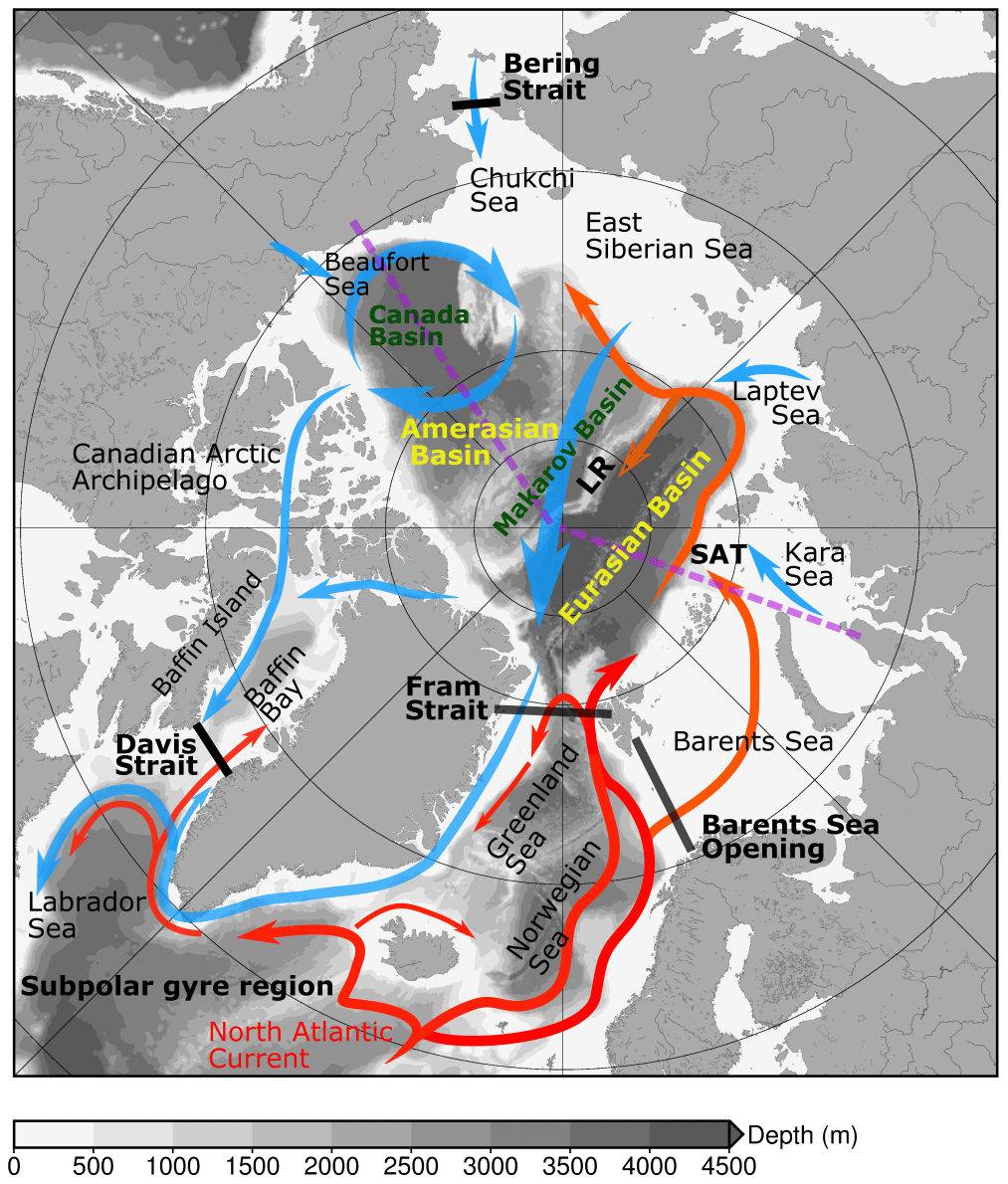
Figure 1Schematic of pan-Arctic Ocean circulations. Blue arrows denote the circulations of low-salinity water, and red arrows denote the circulations of Atlantic water. The background gray color in the ocean denotes bottom bathymetry. The four black lines denote the Arctic gateways of the Bering Strait, Davis Strait, Fram Strait and Barents Sea Opening. The dashed magenta lines indicate the location of the transect shown in Fig. 6. LR and SAT denote Lomonosov Ridge and St. Anna Trough, respectively.
Past model intercomparison studies have revealed large biases and spreads among ocean general circulation models in simulating the hydrography, stratification and gateway transports of the Arctic Ocean. In the Arctic Ocean Model Intercomparison Project (AOMIP), it was identified that a typical issue among regional and global ocean models driven by prescribed atmospheric forcing was an overly thick and deep Atlantic water layer in the Arctic Ocean (Holloway et al., 2007; Karcher et al., 2007), with numerical mixing suggested as the main cause (Holloway et al., 2007). In the subsequent Coordinated Ocean-ice Reference Experiments phase II project (CORE-II; Griffies et al., 2009), it was shown that the global ocean general circulation models used in the Coupled Model Intercomparison Project phase 5 (CMIP5) still struggled with the same issue a decade later when they were forced by prescribed atmospheric forcing (Ilicak et al., 2016). Furthermore, forced simulations of global ocean models used in CMIP6 did not demonstrate significant improvements in representing the Atlantic water layer in the Arctic Ocean and exhibited large spreads in simulated basin mean temperatures (Shu et al., 2023). The model spread (standard deviation among models) of the Atlantic water layer temperature reaches about 1 ∘C, and the multi-model-mean thickness of the Atlantic water layer exceeds twice the observed value (Shu et al., 2023). The two generations of global ocean models used in CMIP5 and CMIP6 also share other common issues, including salinity biases in the Arctic halocline; overestimations of liquid freshwater content; and substantial spreads in ocean volume, heat and freshwater transports in Arctic gateways (Wang et al., 2016a; Ilicak et al., 2016; Shu et al., 2023). The biases identified in forced ocean model simulations were inherited and sometimes exacerbated in coupled climate models of both CMIP5 (Shu et al., 2018, 2019) and CMIP6 (Zanowski et al., 2021; Khosravi et al., 2022; S. Wang et al., 2022; Muilwijk et al., 2023; Heuzé et al., 2023). It was found that ocean models usually perform better in representing the temporal variability of Arctic gateway transports compared to their mean states (Wang et al., 2016a; Shu et al., 2023).
Higher model resolutions have been found to improve certain aspects of Arctic Ocean simulations. The narrowness of the straits in the Canadian Arctic Archipelago makes it challenging to adequately represent the throughflow with the horizontal resolutions typically used in CMIP models. As a result, there are significant model spreads within the ocean models used in CMIP5 and CMIP6 in simulating the volume transport through the Davis Strait (Wang et al., 2016a; Shu et al., 2023). The same issue is present even in ocean models dedicated to Arctic Ocean research (Jahn et al., 2012; Aksenov et al., 2016). However, when the horizontal resolution is increased to approximately 4 km, a forced global ocean model simulation can more accurately reproduce the Canadian Arctic Archipelago throughflow (Wekerle et al., 2013). A low resolution was identified as one of the primary causes of the underestimation of Atlantic Ocean heat transport to the Arctic Ocean in coupled climate models (Docquier et al., 2019). By utilizing variable resolutions that resolve mesoscale eddies regionally (approximately 1 km in the Fram Strait) in a forced global ocean model, the transport of Atlantic water through the Fram Strait can be reasonably reproduced (Wekerle et al., 2017). Furthermore, the model bias of an overly thick Atlantic water layer in the Arctic Ocean, persistently present in previous CMIP ocean models, can be reduced by employing a model horizontal resolution of around 4 km (Wang et al., 2018).
Within the framework of the Ocean Model Intercomparison Project phase 2 (OMIP-2, Griffies et al., 2016), Chassignet et al. (2020) investigated the impact of horizontal resolution on global climate-relevant variables in four pairs of matched low- and high-resolution ocean–sea-ice simulations. They found that typical biases in low-resolution simulations, such as those related to the position, strength and variability of western boundary currents, equatorial currents and the Antarctic Circumpolar Current (identified in previous research by Tsujino et al., 2020), can be significantly improved in high-resolution models. However, the improvements in temperature and salinity vary among different model pairs, and increasing the model resolution (from approximately 1∘ to about 0.1∘) does not consistently lead to bias reduction in all regions for all models (Chassignet et al., 2020). It was also found that increasing the resolution does not consistently improve sea ice concentration and thickness across all the models (Chassignet et al., 2020). In a more recent study focusing on the simulated mixed-layer depth (MLD) in these models, it was shown that increasing the resolution can help reduce MLD biases in deep-water formation regions, particularly in the Northern Hemisphere (Treguier et al., 2023). Neither of these high-resolution studies performed within the OMIP-2 framework specifically focused on the Arctic Ocean.
In this paper, we conducted an assessment of Arctic Ocean simulations using five pairs of matched low- and high-resolution global ocean–sea-ice models. These simulations were driven by the JRA55-do atmospheric state and runoff data set (Tsujino et al., 2018) following the OMIP-2 protocol (Griffies et al., 2016). Unlike previous global model intercomparisons for Arctic Ocean simulations (Wang et al., 2016a, b; Ilicak et al., 2016; Shu et al., 2023), which focused on evaluating low-resolution models that are ocean–sea-ice components of CMIP5 or CMIP6 models, the model pairs used in our study allowed us to specifically investigate the impact of model resolution. The low-resolution cases (1 to ∘) resemble present CMIP6 configurations, while the high-resolution cases (∘ or better) resemble what future CMIP ensemble configurations will be. We evaluated the forced ocean–sea-ice model simulations concerning Arctic Ocean hydrography, the Atlantic water layer, stratification, freshwater content and gateway transports.
The paper is structured as follows. In Sect. 2, we provide a brief description of the models used in this study. Section 3 is dedicated to evaluating the Arctic Ocean simulations and conducting comparisons between models and among model pairs. Finally, we discuss and summarize the results in Sects. 4 and 5.
The models used in this study were forced by version 1.4.0 of the JRA55-do atmospheric forcing data set (Tsujino et al., 2018), covering the period from 1958 to 2018. The OMIP protocol requires the carrying out of simulations with a long spin-up by repeating the forcing for at least five consecutive cycles (Griffies et al., 2016). However, due to the significant computational resources required for high-resolution simulations, previous high-resolution studies within the OMIP-2 framework, such as those of Chassignet et al. (2020) and Treguier et al. (2023), only considered the first cycle and acknowledged that the deep ocean was still far from quasi-equilibrium. In line with these studies, we analyze the Arctic Ocean simulations in the first cycle of the OMIP-2 experiments, making it easier for model groups to participate. Model configurations, including resolutions and parameterizations, were determined by each model group based on their individual development practices. In this paper, the model results are based on monthly model outputs. Table 1 summarizes the five model pairs used in this study, and their corresponding horizontal resolutions are illustrated in Fig. 2.
Table 1Model parameters for the low- and high-resolution configurations.
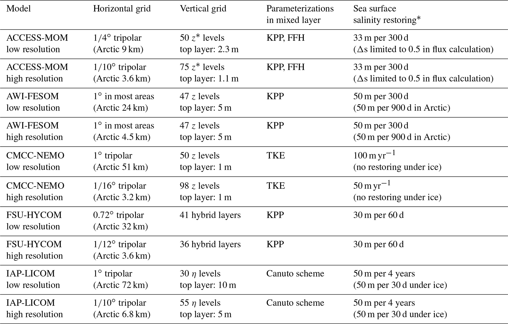
* Unit is practical salinity unit meter per second (psu m s−1).
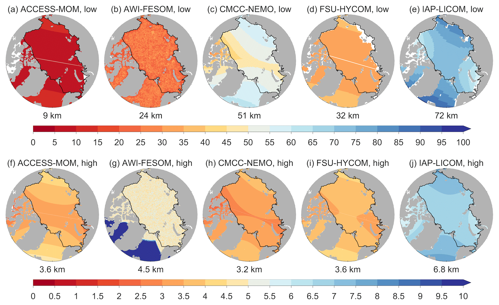
Figure 2Model horizontal grid spacing (in kilometers) in five pairs of models: ACCESS-MOM, AWI-FESOM, CMCC-NEMO, FSU-HYCOM and IAP-LICOM. The black contours indicate the area that is used to calculate the averaged grid size for the Arctic Ocean (denoted under each panel and shown in Table 1).
ACCESS-MOM is the ocean and sea ice component of the Australian Community Climate and Earth System Simulator (ACCESS). It is based on MOM5.1 (Griffies, 2012) at 0.25 and 0.1∘ nominal horizontal grid spacing in the two configurations. These employ tripolar grids, and the mean resolutions in the Arctic Ocean are 9 and 3.6 km, respectively (Fig. 2). The vertical coordinate is z∗, with 50 and 75 levels, respectively. The configurations are described in detail in Kiss et al. (2020), with some updates described in the supplementary material of Solodoch et al. (2022). In both configurations, vertical mixing is parameterized using the K-profile parameterization (KPP; Large et al., 1994), and a parameterization of submesoscale eddy effects in the surface mixed layer (FFH; Fox-Kemper et al., 2008, 2011) is employed. In addition, the Simmons et al. (2004) bottom-enhanced internal tidal mixing and Lee et al. (2006) barotropic tidal mixing are included in both configurations. There is a spatially uniform background vertical diffusivity of 10−6 m2 s−1 at 0.1∘ resolution but none at 0.25∘. The Redi (1982) diffusion and Gent and McWilliams (GM; Gent and McWilliams, 1990) parameterization are used to represent the isoneutral diffusion and thickness diffusivity due to unresolved eddies at 0.25∘, but neither are used at 0.1∘. The sea ice component of ACCESS-MOM is CICE5.1.2 (Hunke et al., 2015), with five thickness categories.
AWI-FESOM, the Finite element/volumE Sea ice–Ocean Model version 2 (Danilov et al., 2017), is a global unstructured-grid ocean general circulation model and serves as the ocean and sea ice component of the Alfred Wegener Institute Climate Model (AWI-CM) (Sidorenko et al., 2019; Streffing et al., 2022). The model resolution is 1∘ in most global ocean areas and is refined to 24 km north of 45∘ N. The two configurations differ only in the horizontal resolution in the Arctic Ocean, with grid spacings of 24 and 4.5 km, respectively. Both configurations employ 47 z levels. Vertical mixing is parameterized using the KPP scheme, with background diffusivity of m2 s−1 in the Arctic region. Redi diffusion and the GM parameterization are employed but are deactivated in regions where the horizontal grid spacing is less than half the first baroclinic Rossby radius of deformation. The Redi diffusivity and GM coefficient are scaled with grid spacing in the horizontal and vary vertically based on the squared buoyancy frequency (Ferreira et al., 2005; Danabasoglu and Marshall, 2007). The sea ice component of AWI-FESOM is FESIM2 (Danilov et al., 2015).
CMCC-NEMO, the Nucleus for the European Modelling of the Ocean (NEMO) version 3.6 (Madec and the NEMO team, 2016), serves as the ocean and sea ice component of the CMCC climate model (CMCC-CM) (Cherchi et al., 2019). It employs tripolar grids with nominal horizontal resolutions of 1 and ∘ for the two configurations. The corresponding mean resolutions are 51 and 3.2 km in the Arctic Ocean. The model utilizes 50 and 98 z levels in the two configurations, respectively. Vertical mixing coefficients are calculated using the turbulent kinetic energy (TKE) parameterization introduced by Blanke and Delecluse (1993), which incorporates the effects of Langmuir cells and surface wave breaking (Madec and the NEMO team, 2016). The background vertical diffusivity is and m2 s−1 in the low- and high-resolution configurations, respectively. In the low-resolution configuration, Redi and GM diffusivity coefficients are scaled with grid spacing, while the high-resolution configuration employs biharmonic viscosity and diffusion for lateral mixing, with coefficients varying as the cube of the grid size (Iovino et al., 2023). The low-resolution configuration employed CICE4 (Hunke and Lipscomb, 2010) as its sea ice component, while the high-resolution configuration employed LIM2 (Timmermann et al., 2005).
FSU-HYCOM, a global version of the HYbrid Coordinate Ocean Model (HYCOM) (Chassignet et al., 2003), employs tripolar grids with horizontal resolutions of 0.72 and ∘ for two configurations, corresponding to mean resolutions of 32 and 3.6 km in the Arctic Ocean. The model employs 41 and 36 hybrid coordinate layers in the low- and high-horizontal-resolution configurations, respectively. Vertical mixing is parameterized using the KPP scheme, with background diffusivity of m2 s−1. In the low-resolution configuration, interface height smoothing, equivalent to the GM diffusion, is achieved using a biharmonic operator with a mixing coefficient determined by the grid spacing multiplied by a velocity scale of 0.02 m s−1, except in the North Pacific and North Atlantic, where a Laplacian operator with a velocity scale of 0.01 m s−1 is employed. In the high-resolution configuration, interface height smoothing utilizes a biharmonic operator with a velocity scale of 0.015 m s−1. The sea ice component of FSU-HYCOM is CICE4 (Hunke and Lipscomb, 2010).
IAP-LICOM, the LASG/IAP Climate system Ocean Model (LICOM) version 3 (Li et al., 2020b; Lin et al., 2020), is the ocean and sea ice component of the Flexible Global Ocean–Atmosphere–Land System model (FGOALS) and the Chinese Academy of Sciences Earth System Model (CAS-ESM) (Li et al., 2020a; Bao et al., 2013). It employs tripolar grids with nominal horizontal resolutions of approximately 1 and ∘ for two configurations, resulting in mean resolutions of 72 and 6.8 km in the Arctic Ocean. The model adopts the η vertical coordinate (Mesinger and Janjic, 1985), utilizing 30 and 55 levels in the respective configurations. Mixing is parameterized using the scheme proposed by Canuto et al. (2002), with background diffusivity of m2 s−1. In addition, the St Laurent et al. (2002) tidal-mixing scheme is employed. In the low-resolution configuration, isoneutral diffusion and GM parameterization are employed, with diffusivity coefficients scaled vertically based on the squared buoyancy frequency (Ferreira et al., 2005). The sea ice component of IAP-LICOM is CICE4 (Hunke and Lipscomb, 2010). The high-resolution IAP-LICOM solely incorporates the thermodynamic part of CICE4, lacking its sea ice dynamics.
Sea ice properties are not a focus of this paper. Arctic and Antarctic sea ice concentrations and thicknesses in March and September have been discussed in the same model pairs (Chassignet et al., 2020) and/or in the corresponding model description papers cited above. To summarize previous findings briefly, March Arctic sea ice concentration fields are similar among the models at all resolutions, and September Arctic sea ice concentration fields are more sensitive to models than to spatial resolutions. Sea ice thicknesses differ considerably among the models in all seasons. Overall, increasing the resolution did not remarkably improve sea ice in these simulations.
In this study, the Arctic Ocean is defined as the Arctic area enclosed by the Fram Strait, the Barents Sea Opening, the Bering Strait and the northern boundary of Canadian Arctic Archipelago, and the Eurasian Basin and Amerasian Basin are defined as the deep Arctic Ocean areas with bottom topography deeper than 500 m, separated by the Lomonosov Ridge.
3.1 Mean hydrography
3.1.1 Temperature
We utilize the PHC3.0 hydrography climatology (Steele et al., 2001) to assess the basin mean temperature and salinity. According to the PHC3.0 climatology, the warm Atlantic water layer (warmer than 0 ∘C) is situated beneath the cold surface water, spanning a depth range of approximately 150–800 m (Fig. 3). The maximum temperature is located in the depth range of approximately 200–400 and 400–600 m in the Eurasian and Amerasian basins, respectively. Since PHC3.0 primarily relies on observations from the 1970s to the 2000s, we compare the model results averaged over the period from 1971 to 2000 to assess their agreement with PHC3.0.
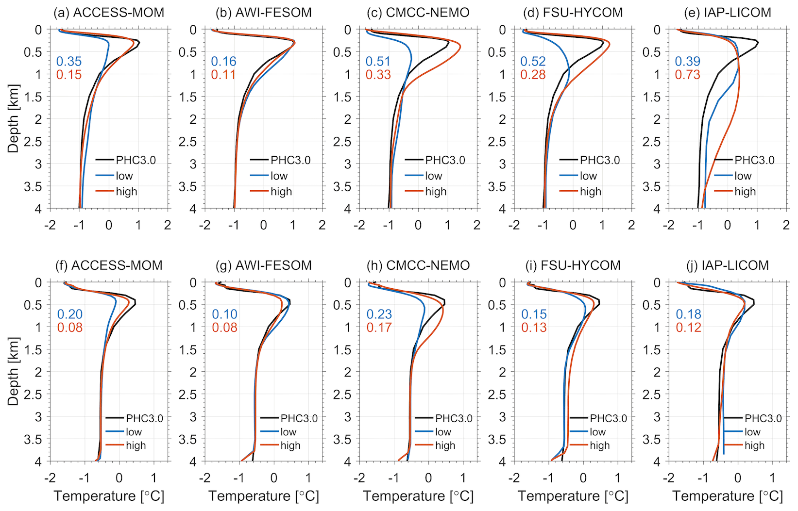
Figure 3Basin mean potential temperature profiles for the (a–e) Eurasian Basin and (f–j) Amerasian Basin from the five models at low (blue) and high (red) resolution compared to the PHC3.0 hydrography climatology (black; Steele et al., 2001). The model results are averaged over 1971–2000. The Atlantic water layer is characterized as the warm oceanic layer bounded by the 0 ∘C isotherm. The root-mean-square errors for the upper 3500 m depth are displayed in each panel.
In the Eurasian Basin, four out of five low-resolution models (except for AWI-FESOM) underestimate the maximum temperature of the Atlantic water layer and overestimate the temperature below the Atlantic water layer (Fig. 3, upper panels). The warm biases extend to at least 2500 m depth in these models. Three high-resolution configurations (namely ACCESS-MOM, CMCC-NEMO and FSU-HYCOM) exhibit notable improvements with higher maximum temperatures compared to their low-resolution counterparts. The warm biases in the deeper ocean are also reduced in two models (ACCESS-MOM and CMCC-NEMO). Both configurations of AWI-FESOM faithfully represent the temperature in the Eurasian Basin, with warm bias in the 500–1500 m depth range and lower in its high-resolution configuration.
In the Amerasian Basin, the simulated maximum temperature aligns more closely with observations as the horizontal resolution increases (particularly in ACCESS-MOM, CMCC-NEMO and FSU-HYCOM; Fig. 3, lower panels). However, in two of these models (CMCC-NEMO and FSU-HYCOM), the high-resolution configuration exhibits larger warm biases below 600 m depth compared to the low-resolution configuration. In AWI-FESOM, with higher resolution, the warm bias below 600 m depth is reduced, although a slight cold bias emerges at the depth of maximum temperature. Considering temperature in the upper 3500 m depth range, the root-mean-square error (RMSE, displayed in each panel of Fig. 3) indicates that increasing the resolution effectively reduces the overall model biases (evident in four out of five models).
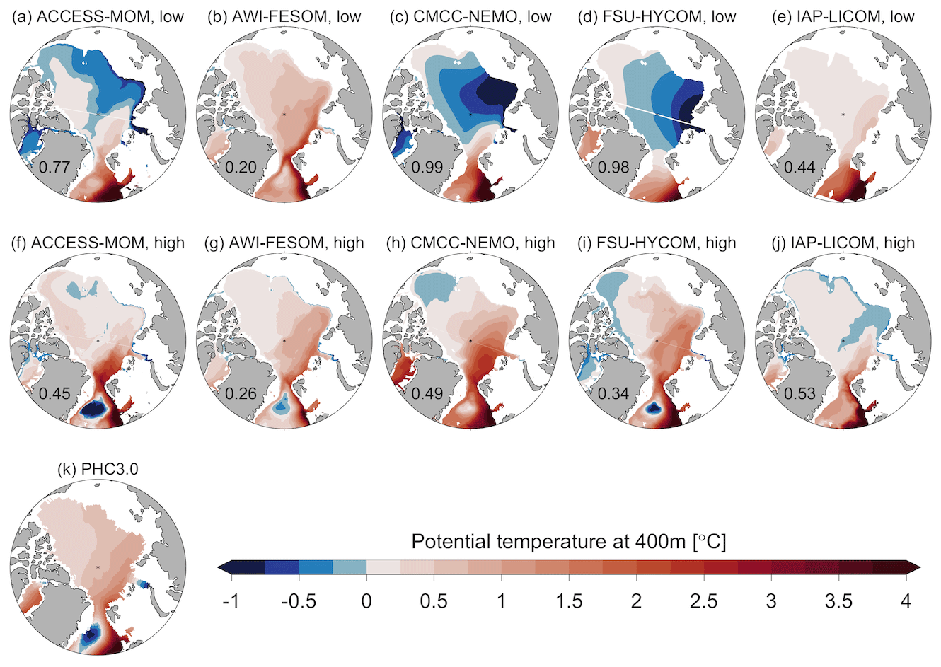
Figure 4Spatial distribution of the simulated potential temperature at 400 m depth averaged over 1971–2000: (a–e) low-resolution models versus (f–j) high-resolution models. The PHC3.0 temperature climatology (Steele et al., 2001) at 400 m depth is shown in (k). The model root-mean-square errors for temperature at 400 m depth in the Arctic deep basin (region with bottom topography deeper than 500 m) are displayed in each respective panel.
The temperature maps at a depth of 400 m provide insight into the spatial distribution of the warm Atlantic water in the deep basin of the Arctic (Fig. 4). Observational climatology shows that the warm Atlantic water enters the Arctic basin through the Fram Strait and circulates in a cyclonic direction within the basin (Fig. 4k). However, four low-resolution models (except for AWI-FESOM) exhibit lower temperatures north of Svalbard compared to the observational climatology, indicating a deficiency in the inflow of warm Atlantic water through the Fram Strait in these models. Additionally, these four models show a prominent cold bias in the eastern Eurasian Basin, with three of them even displaying negative values (Fig. 4a, c, d). The maps of Atlantic water core temperature (AWCT), representing the maximum temperature throughout the water column in areas with bottom topography deeper than 150 m, demonstrate the absence of warm Atlantic water in the eastern Eurasian Basin and its downstream region in these models (Fig. 5a, c, d). This cold bias can be traced back to the Barents Sea branch of the Atlantic water inflow, where the temperature is much colder in these three models compared to in other models and their high-resolution counterparts. Hence, the cold biases in the deep basin of the Arctic can be attributed to both insufficient inflow of warm water through the Fram Strait and excessive discharge of cold water from the St. Anna Trough, consistently with findings from previous model intercomparison studies (Ilicak et al., 2016; Shu et al., 2019). In the high-resolution configurations, both issues are mitigated, resulting in a significant reduction in the cold bias in the deep basin (Fig. 5f, h, i).
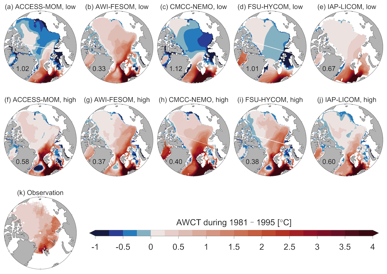
Figure 5Simulated Atlantic water core temperature (AWCT) averaged over 1981–1995: (a–e) low-resolution versus (f–j) high-resolution simulations. (k) The AWCT for the same period based on observations (Polyakov et al., 2020). The model root-mean-square errors for AWCT in the Arctic deep basin (region with bottom topography deeper than 500 m) are displayed in each respective panel.
Both the temperature at 400 m depth and the AWCT demonstrate that, in the high-resolution configurations of AWI-FESOM and FSU-HYCOM, the Atlantic water extends along the continental slope all the way to the Laptev Sea, with a portion of it recirculating along the Lomonosov Ridge (Figs. 4g, i and 5g, i), which is consistent with observations (Woodgate et al., 2001; Richards et al., 2022). Similar improvement in simulating the spatial pattern of the warm Atlantic water is not seen in other models. The high-resolution configurations of ACCESS-MOM and CMCC-NEMO exhibit a broad Atlantic water flow from the Fram Strait into the Eurasian Basin instead of a distinct inflow branch along the continental slope (Figs. 4f, h and 5f, h).
Overall, the RMSE for the AWCT (displayed in each panel of Fig. 5) suggests that increasing resolution improves the representation of the Arctic Atlantic water layer (in four out of five models). AWI-FESOM exhibits the smallest RMSE in both versions. However, its high-resolution version shows a slightly larger RMSE than the low-resolution version, primarily due to a relatively small cold bias in the Amerasian Basin in its high-resolution version (Fig. 5b, g).
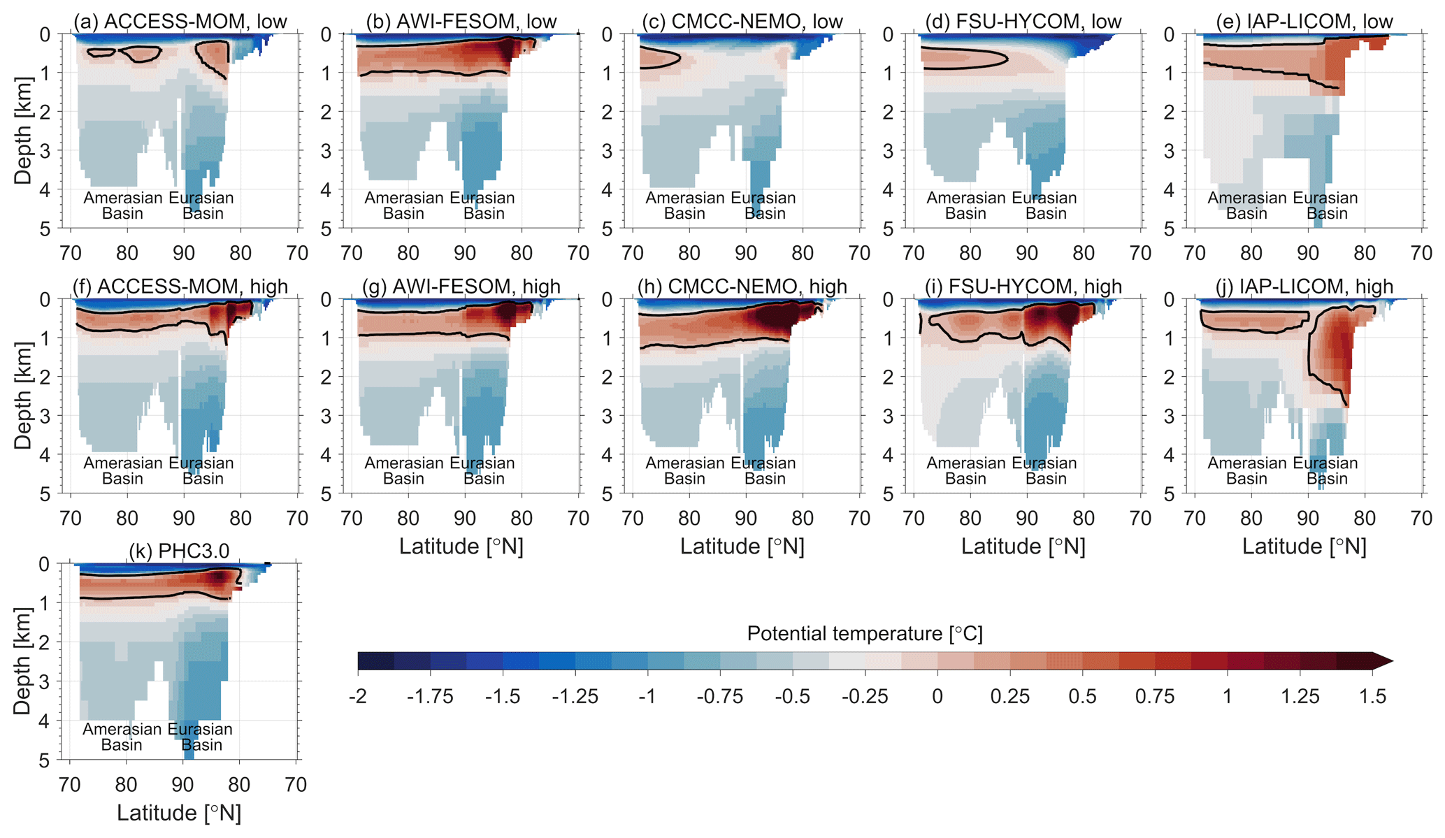
Figure 6Potential temperature in a vertical transect crossing the Arctic basin averaged over 1971–2000: (a–e) low-resolution versus (f–j) high-resolution simulations. The PHC3.0 temperature climatology (Steele et al., 2001) is shown in (k). The boundary of the Atlantic water layer, the 0 ∘C isotherm, is indicated by black contour lines. The transect is along the longitudes of 145∘ W and 70∘ E, and its location is indicated in Fig. 1.
Fig. 6 depicts the vertical transect of temperature across the Arctic Ocean. According to the PHC3.0 climatology, the warm Atlantic water layer exhibits a deepening upper boundary (0 ∘C isotherm) from the Eurasian Basin to the Amerasian Basin (Fig. 6k). It also indicates that the intermediate and deep layers (located below the lower 0 ∘C isotherm) are warmer in the Amerasian Basin compared to in the Eurasian Basin. The cold deep water in the Eurasian Basin, mainly sustained by dense shelf waters and entrained ambient waters when they sink on the continental slope, can only overflow to the Amerasian Basin through the central part of the Lomonosov Ridge (Rudels and Quadfasel, 1991; Jones et al., 1995). Among the low-resolution models, only one model (AWI-FESOM) successfully simulates a warm Atlantic water layer with a depth range and temperature magnitude similar to the observations (Fig. 6b). Encouragingly, three models (ACCESS-MOM, CMCC-NEMO and FSU-HYCOM) demonstrate the ability to simulate the Atlantic water layer more accurately when their resolutions are increased despite some biases in layer thickness (i.e., too thin in ACCESS-MOM and too thick in CMCC-NEMO and FSU-HYCOM) (Fig. 6f, h, i). However, the high-resolution IAP-LICOM exhibits an excessively thick Atlantic water layer in the Eurasian Basin (Fig. 6j). Additionally, its Atlantic water layer is split into two cells due to a cold tongue recirculating along the Lomonosov Ridge (Fig. 4j). The degradation of the IAP-LICOM simulation at high resolution is likely due to the misrepresentation of sea ice and, thus, unrealistic surface momentum and buoyancy fluxes, resulting from the absence of sea ice dynamics in the model (Chassignet et al., 2020). All the models successfully reproduce the temperature contrast in the deep ocean between the two basins (Fig. 6). Below 1000 m depth in the Amerasian Basin, the high-resolution FSU-HYCOM exhibits a notable warm bias that is absent in its low-resolution counterpart (Fig. 6i). This bias is likely due to the lower vertical resolution in the high-resolution configuration of FSU-HYCOM than in its low-resolution configuration (Table 1).
3.1.2 Salinity
Figure 7 illustrates the simulated salinity profiles in the two basins, and the corresponding salinity biases are shown in Fig. S1 in the Supplement. All the models tend to exhibit a negative salinity bias in the halocline below the surface layer. This bias is likely caused by excessive vertical mixing in the models, which reduces salinity in the halocline and increases it near the surface (Wang et al., 2018). To mitigate the issue of large drift in ocean salinity and circulation, global models typically restore sea surface salinity to climatology (Griffies et al., 2009). The restoring can dampen the increase in surface salinity induced by vertical mixing. As a result of sea surface salinity restoring and vertical mixing, the mean salinity is underestimated, as is evident from the overestimation of liquid freshwater content (see Sect. 3.4). This issue was previously investigated in the CORE-II Arctic Ocean study (Wang et al., 2016a), and it appears that the state-of-the-art ocean models in OMIP-2 still encounter the same challenge as the CORE-II models.
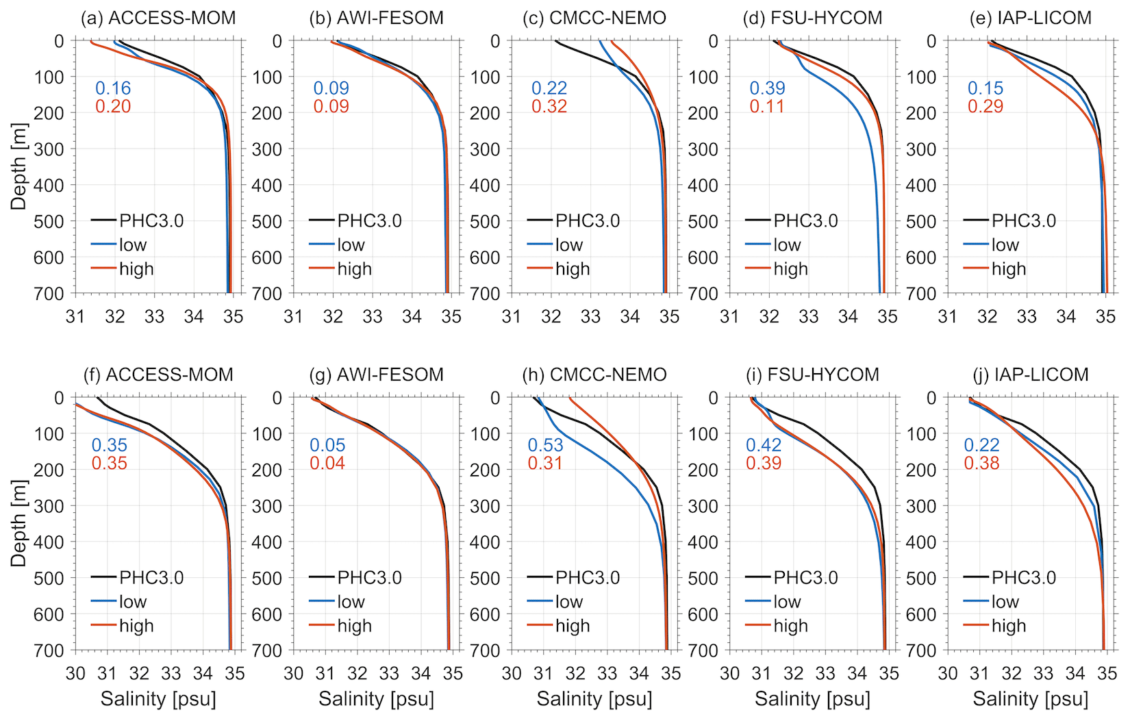
Figure 7Basin mean salinity for (a–e) the Eurasian Basin and (f–j) the Amerasian Basin in the five models at low (blue) and high (red) resolution compared to the PHC3.0 hydrography climatology (black; Steele et al., 2001). Model results are averaged over 1971–2000. The root-mean-square errors for the upper 700 m depth are displayed. The plots of salinity biases are shown in Fig. S1.
It is encouraging to observe that the high-resolution configurations exhibit smaller salinity biases in the halocline in all models except for IAP-LICOM, primarily in the Eurasian Basin (Figs. 7 and S1). Previous studies have suggested that an inadequate treatment of brine rejection could lead to static instability and excessive vertical mixing over a wide depth range, resulting in a negative salinity anomaly in the halocline and a positive salinity anomaly at the surface (Nguyen et al., 2009). However, our findings indicate that increasing model resolution can reduce the negative salinity bias in the halocline, suggesting that at least part of this bias is unrelated to the treatment of brine rejection in the models as none of the models analyzed in this study employed brine rejection parameterization for the Arctic Ocean. On the other hand, salinity biases at the ocean surface are amplified in two high-resolution models (CMCC-NEMO and ACCESS-MOM, Fig. 7a, c, h), which could be attributed to the limited sea surface salinity restoration in these models (Table 1). IAP-LICOM displays larger salinity biases throughout the ocean column in its high-resolution configuration compared to its low-resolution configuration (Fig. 7e, j).
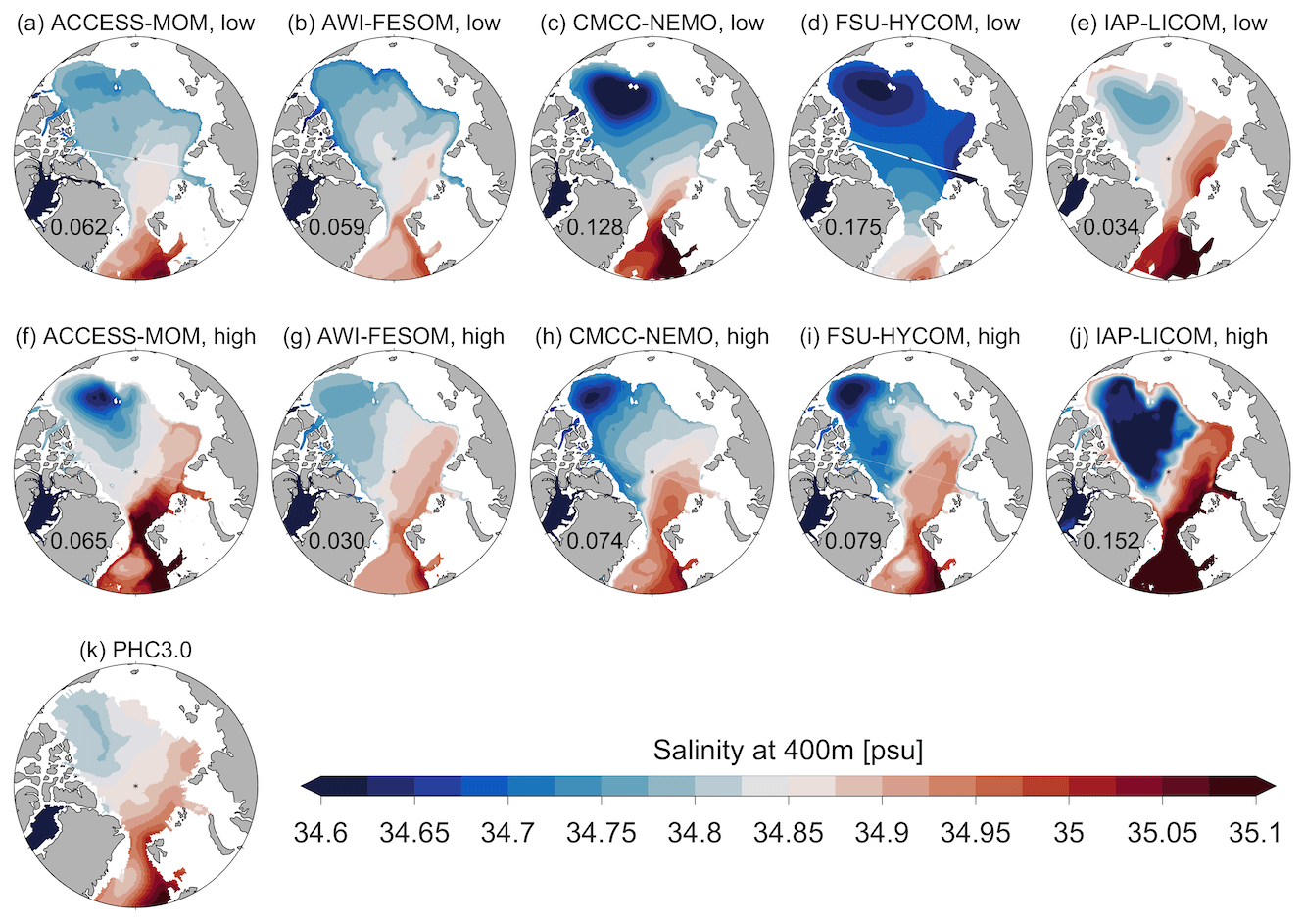
Figure 8Simulated salinity at 400 m depth averaged over 1971–2000: (a–e) low-resolution models versus (f–j) high-resolution models. The PHC3.0 salinity climatology (Steele et al., 2001) at 400 m depth is shown in (k). The model root-mean-square errors for salinity at 400 m depth in the Arctic deep basin (region with bottom topography deeper than 500 m) are displayed in each respective panel.
Similarly to the spatial pattern of temperature (Fig. 4k), the spatial pattern of salinity at 400 m depth illustrates the cyclonic circulation of the Atlantic water along the continental slope (Fig. 8k). The Canada Basin displays the lowest salinity at this depth, reflecting the deepening of the isohaline due to Ekman convergence induced by the Beaufort High sea level pressure (Proshutinsky et al., 2002, 2009; Wang and Danilov, 2022; Timmermans and Toole, 2023). Most of the model simulations are able to capture the basic salinity contrast between the Eurasian Basin and the Amerasian Basin (Fig. 8). The low-resolution configuration of FSU-HYCOM exhibits relatively large negative biases in salinity throughout the deep basin at 400 m depth (Fig. 8d). It fails to simulate the Atlantic water boundary current entering the basin through the Fram Strait, which carries warm, saline Atlantic water in reality. However, its high-resolution configuration shows an improved representation of the Atlantic water inflow and, consequently, a better representation of salinity in the Eurasian Basin (Fig. 8i). Nevertheless, its salinity in the Canada Basin remains biased low. The high-resolution configurations of ACCESS-MOM and CMCC-NEMO also demonstrate better simulation of salinity in the Eurasian Basin compared to their low-resolution counterparts, but their salinity in the Canada Basin is still biased low (Fig. 8f, h), similarly to the high-resolution FSU-HYCOM. In AWI-FESOM, the cyclonic circulation of the Atlantic water is better simulated with a higher resolution (Fig. 8b, g). Some of the Atlantic water directly penetrates towards the North Pole and Amerasian Basin in its low-resolution configuration, and this issue is resolved in the high-resolution configuration. As the vertical resolution is the same in both AWI-FESOM configurations, the improved model performance can be attributed to higher horizontal resolution. The salinity bias in IAP-LICOM is more pronounced in its high-resolution configuration for both basins (Fig. 8e, j), likely due to the impact of misrepresented sea ice cover, as mentioned above.
The RMSE of the salinity at 400 m depth (displayed in each panel of Fig. 8) indicates that the overall salinity biases in the Atlantic water layer are notably reduced in three out of five high-resolution models. However, for the overall salinity biases in the upper 700 m depth range, there is no consistent improvement with increasing resolution in the models, as indicated by the RMSE displayed in each panel of Fig. 7.
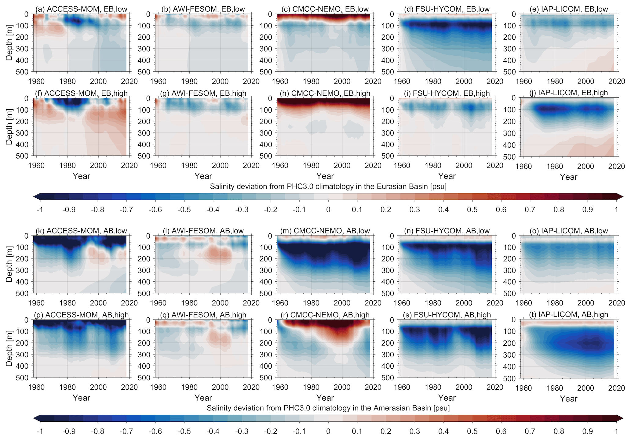
Figure 9Depth–time plot of basin mean salinity deviation from PHC3.0 climatology in the (upper two rows) Eurasian Basin and (lower two rows) Amerasian Basin; (a)–(e) and (k)–(o) are for the low-resolution models, and (f)–(j) and (p)–(t) are for the high-resolution models.
Despite some improvements in representing salinity in high-resolution models, as described above, it is important to acknowledge that the salinity biases in most of these models (particularly in the halocline and/or surface layer) still exceed the magnitudes of salinity changes observed over decades, as shown in Fig. 9. In several models with significant salinity biases (up to approximately 1 psu), these biases escalate to high levels within the first few years of the model simulations. In certain cases, such as the low-resolution FSU-HYCOM model, the fresh biases persist and extend downwards throughout the entire simulation period (Fig. 9d, n). Background vertical diffusivity employed in models can significantly influence the vertical distribution of salinity and the stratification in the Arctic Ocean (Zhang and Steele, 2007). The underlying cause for the larger fresh biases in the halocline of FSU-HYCOM compared to AWI-FESOM could partially be attributed to the background diffusivity within the KPP mixing scheme. In FSU-HYCOM, the background diffusivity is m2 s−1, which is approximately 1 order of magnitude higher than that of AWI-FESOM ( m2 s−1). However, in the case of IAP-LICOM, which has a relatively small background diffusivity of m2 s−1, the fresh biases remain substantial (Fig. 9e, j, o, t). Therefore, it is evident that other factors, such as explicit mixing from applied parameterizations and spurious numerical mixing, also contribute to the salinity biases.
3.2 Warming events in Atlantic water layer
Observations have revealed several warming events in the Arctic Atlantic water layer, which are associated with strengthened ocean heat influxes through the Fram Strait. These events occurred in the 1990s and the 2010s (Steele and Boyd, 1998; Gerdes et al., 2003; Karcher et al., 2012; Polyakov et al., 2012, 2020; Wang et al., 2020b). The abnormally high North Atlantic Oscillation in the 1990s strengthened the Atlantic water boundary current in the Nordic Seas and increased the inflow through the Fram Strait (Dickson et al., 2000). Simultaneously, the positive Arctic Oscillation strengthened the cyclonic circulation within the Arctic Ocean and facilitated the influx of Atlantic water from the Fram Strait (Wang et al., 2023). During the 2010s, both the warming and intensification of the inflow in the Fram Strait due to Arctic sea ice decline, which maintained the strength of the cyclonic Greenland Sea gyre circulation by reducing sea ice freshwater export through the Fram Strait, contributed to the warming of the Atlantic water layer in the Arctic basin (Wang et al., 2020b). The observed ocean warming not only manifests changes in the coupled air–ice–sea system but also influences the marine ecosystem in the region. Hence, it is important to assess whether the OMIP-2 models, driven by the same atmospheric forcing, are capable of reasonably reproducing the warming events.
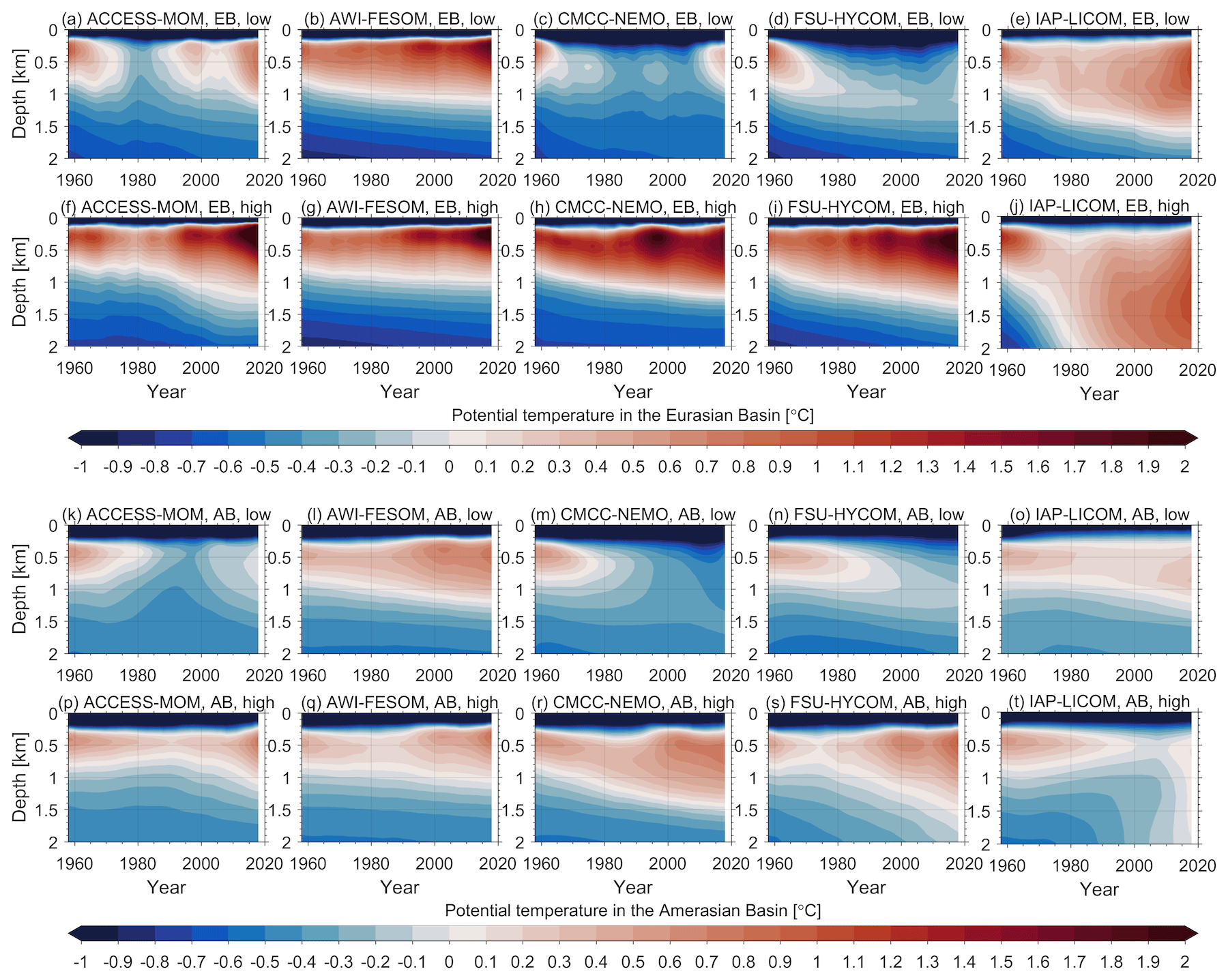
Figure 10Depth–time plot of basin mean potential temperature of the (upper two rows) Eurasian Basin and (lower two rows) Amerasian Basin; (a)–(e) and (k)–(o) are for the low-resolution models, and (f)–(j) and (p)–(t) are for the high-resolution models.
Figure 10 presents the depth–time plot of basin mean temperature in the Eurasian and Amerasian basins. In the low-resolution models, AWI-FESOM successfully reproduces the warming events in the Eurasian Basin (Fig. 10b). ACCESS-MOM and CMCC-NEMO exhibit signals of these warming events in their low-resolution configurations but with lower magnitudes (Fig. 10a, c). This is consistent with their cold bias in simulated mean temperature (Figs. 4 and 5). The 1990s warming is absent in the low-resolution FSU-HYCOM and IAP-LICOM (Fig. 10d, e). Among the high-resolution models, with the exception of IAP-LICOM, all are capable of reproducing the two warming events in the Eurasian Basin (Fig. 10f–j). The thickening trend of the warm Atlantic water layer (indicated by the deepening trend of the lower boundary of the warm Atlantic water layer) remain large in four of the high-resolution models (Fig. 10f–j).
The warming in the Eurasian Basin propagates into the Amerasian Basin with a time lag of a few years (Steele and Boyd, 1998; Polyakov et al., 2012). Since most of the low-resolution models fail to accurately reproduce the two warming events in the Eurasian Basin, they do not exhibit both warming events in the Amerasian Basin (Fig. 10k, m–o). In contrast, all the high-resolution configurations, except for IAP-LICOM, can simulate the warming events in the Amerasian Basin, with a time lag of about 4 years compared to the Eurasian Basin (Fig. 10p–s).
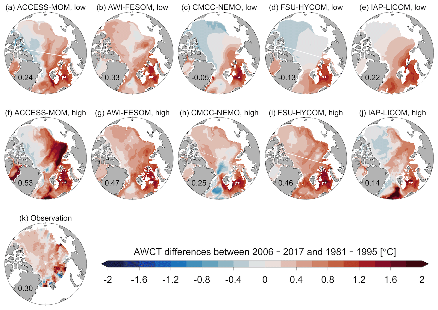
Figure 11Difference in the Atlantic water core temperature (AWCT) between 2006–2017 and 1981–1995 in the models (a–j) and observations (k) (Polyakov et al., 2020). The AWCT in these two periods is shown in Figs. 5 and S2, respectively. The mean values averaged over the Arctic deep basin (region with bottom topography deeper than 500 m) are displayed in each respective panel.
Hydrography observations in the Arctic Ocean are relatively sparse in time and space, leading to large uncertainty in gridded temperature data based on these observations. With this limitation in mind, we utilize the gridded AWCT averaged over two periods (1981–1995 and 2006–2017), available from Polyakov et al. (2020), to evaluate the simulated AWCT changes in the models. Figure 11 presents the difference in AWCT between these two periods for both the observation and the model simulations. The observations indicate a clear increase in AWCT in most areas of the Arctic basin (Fig. 11k). Inconsistently, four out of the five low-resolution models simulate a reduction in AWCT in a large part of the Arctic basin. Averaged over the Arctic deep basin, the observation indicates an increase of 0.3 ∘C in the AWCT between the two considered periods, while two of the low-resolution models (CMCC-NEMO and FSU-HYCOM) simulated a reduction in the AWCT (Fig. 11c, d).
The high-resolution FSU-HYCOM demonstrates an increase in the AWCT between the two periods across the basin and, thus, an evident improvement (Fig. 11i). The high-resolution CMCC-NEMO also better represents the AWCT change in the Amerasian Basin compared to its low-resolution counterpart, although it exhibits an erroneous cooling anomaly in the Eurasian Basin (Fig. 11h), potentially attributed to the excessively strong warming in the 1990s simulated by high-resolution CMCC-NEMO (Fig. 10h). Neither ACCESS-MOM nor IAP-LICOM show noticeable improvement in simulating the rise of AWCT in the Amerasian Basin in their high-resolution configurations (Fig. 11f, j). These models seem to struggle with advecting the signal of Atlantic water warming into the Amerasian Basin, which could be explained by the presence of a too-large and too-strong anticyclonic Beaufort Gyre, indicated by the excess freshwater content (see Sect. 3.4). This is linked to the fact that the upper-ocean circulation has a strong imprint on the Atlantic water layer circulation (Lique et al., 2015; Hinrichs et al., 2021; Wang et al., 2023). In all the high-resolution models, the AWCT difference between the two periods averaged over the Arctic deep basin is positive. However, three of these models tend to overestimate this difference in comparison with the available observational estimate.
3.3 Mixed-layer depth and cold halocline base depth
The winter mixed-layer depth (MLD) in the Barents Sea is deeper than in the Arctic deep basin (Peralta-Ferriz and Woodgate, 2015), reflecting the strong heat loss from the warm Atlantic water to the atmosphere in the Barents Sea (Schauer et al., 1997; Smedsrud et al., 2013; Shu et al., 2021). In the Arctic deep basin, the MLD remains relatively shallow even during winter due to the presence of low-salinity water at the surface. The winter MLD is not only a climate-relevant variable but also an important factor that regulates summer primary production in the Arctic (Popova et al., 2010). Between the surface mixed-layer and the Atlantic water layer lies the Arctic halocline, which acts as an insulating layer, inhibiting the transfer of heat from the Atlantic water layer to the cold mixed layer and sea ice. An uplift of the boundary between the halocline and Atlantic water layer, accompanied by a weakening of the halocline stratification and warming of the Atlantic water layer, was observed in the eastern Eurasian Basin in the 2010s (Polyakov et al., 2017, 2020). This phenomenon, known as Arctic Atlantification (Polyakov et al., 2017), is primarily driven by the decline in Arctic sea ice (Wang et al., 2020b). In the following, we will evaluate the simulations of the MLD and halocline base depth in the models.
3.3.1 Winter MLD
When determining the MLD in the Arctic Ocean based on observations, MLD is defined as the depth at which potential density exceeds the density of the shallowest measurement (considered to be the best estimate for surface density) by 0.1 kg m−3 (Peralta-Ferriz and Woodgate, 2015). Note that observational profiles with a shallowest measurement deeper than 10 m are typically excluded from consideration because MLDs shallower than 10 m may occur during certain seasons and in some regions of the Arctic Ocean (Peralta-Ferriz and Woodgate, 2015). We follow this MLD definition and compute the MLD referenced to surface density using monthly mean temperature and salinity from the models while noting the cautionary remarks in Treguier et al. (2023) about how MLD calculated from monthly mean data will differ from higher-frequency data.
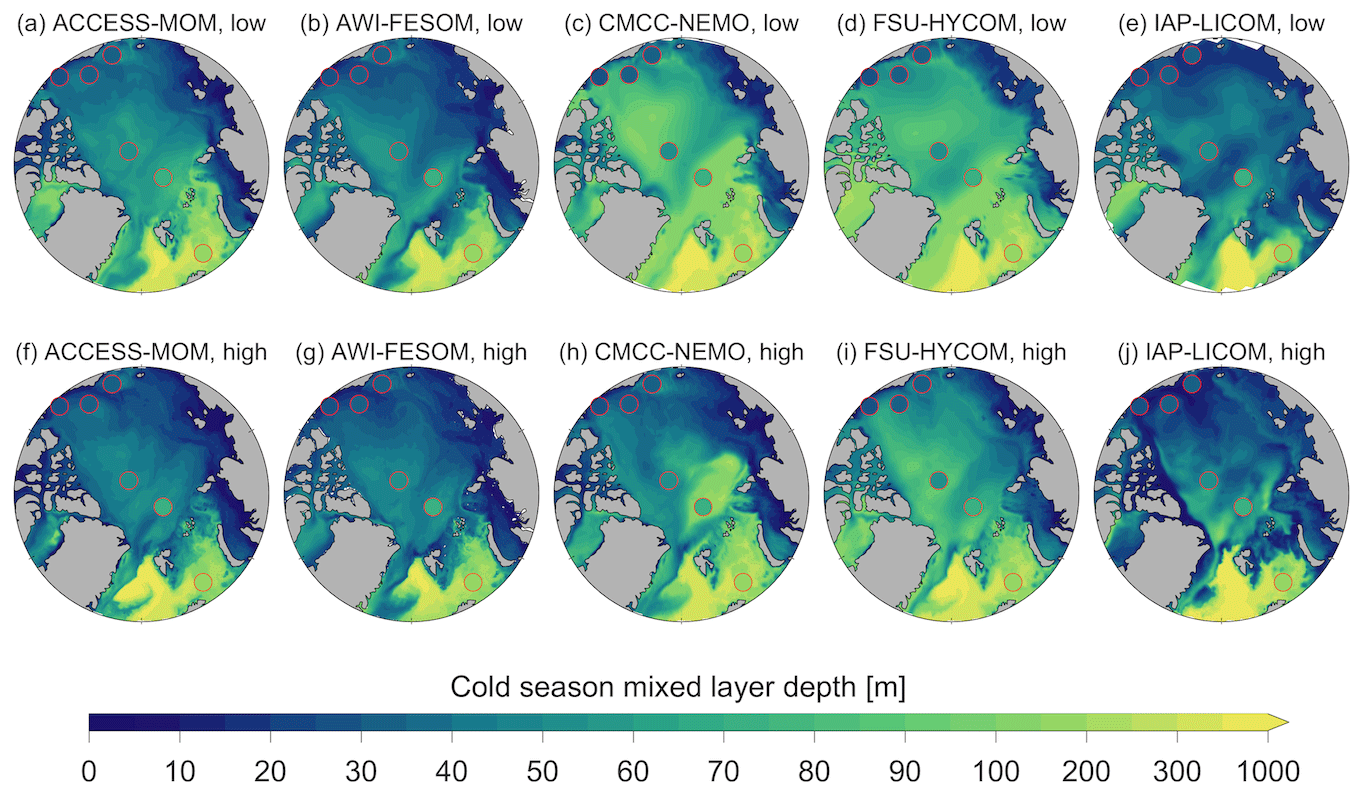
Figure 12Mixed-layer depth (MLD) in the cold season (November to May) averaged over 1979–2012. The observational estimates for six regions are shown as filled circles (Peralta-Ferriz and Woodgate, 2015). The color bar scaling is nonuniform.
Figure 12 depicts the MLD in winter (November to May) during the period 1979–2012 for each model, along with the observational estimates (averaged over six Arctic regions, shown as circles; Peralta-Ferriz and Woodgate, 2015). The observational estimates indicate that the winter MLD is approximately 30 m in the southern Beaufort Sea, Canada Basin and Chukchi Sea; approximately 50 m in the Makarov Basin; around 70 m in the Eurasian Basin; and roughly 170 m in the Barents Sea. Three models (ACCESS-MOM, AWI-FESOM and IAP-LICOM) can reproduce the contrast between the deep MLD in the Barents Sea and the shallow MLD in the Arctic deep basin in both configurations (Fig. 12a, b, e, f, g, j). Increasing horizontal resolution leads to a reduction in MLD of 10–20 m in most of the Arctic deep-basin area in these models. Mesoscale eddies have an effect on restratifying the mixed layer, thereby reducing the MLD (Treguier et al., 2023). The resolutions used in the high-resolution OMIP-2 configurations (3–6 km, Fig. 2) are only eddy-permitting in the Arctic deep basin (Wang et al., 2020a). The comparison in Fig. 12 indicates that the high-resolution configurations may capture some of the eddy effects, although eddies are not fully resolved yet. They slightly underestimate the observations in the Eurasian Basin by about 20 m. However, as the MLD computed from monthly temperature and salinity tends to be shallower than that computed from snapshot profiles due to the nonlinearity of the MLD (Treguier et al., 2023), we cannot conclude that these high-resolution configurations have a worse MLD than the low-resolution ones.
The other two models (CMCC-NEMO and FSU-HYCOM) simulate too-deep MLDs in both the Eurasian and Amerasian basins in their low-resolution configurations (Fig. 12c, d). This overestimation can be attributed to stratification biases in the upper ocean within these models. Specifically, they demonstrate either positive salinity biases at the surface (see Fig. 9c) or negative salinity biases in the subsurface (see Fig. 9d, m, n). Such salinity biases lead to reduced stratification, consequently promoting the formation of deeper mixed layers during wintertime. Our finding is consistent with previous research, which highlighted the dominating impact of the simulated salinity profile and, consequently, density stratification on the models' performances in simulating winter MLD (Allende et al., 2023). In the high-resolution configurations of these two models, there is a partial improvement in the MLD estimation within certain regions of the Arctic deep basin (Fig. 12h, i). However, this improvement does not correspond to a reduction in salinity biases. For example, the significant fresh bias observed in the subsurface of the Amerasian Basin in the low-resolution CMCC-NEMO model is replaced by a positive salinity bias at the surface in its high-resolution counterpart (Fig. 9m, r). The salinity biases in different depth ranges are altered in such a manner that the overall upper-ocean stratification in the Amerasian Basin is enhanced, resulting in a shallower MLD than in the low-resolution configuration (Fig. 12h). Similarly, the decrease in the MLD in the high-resolution FSU-HYCOM model (Fig. 12i) can be partially explained by the amplified fresh bias at the surface (comparing Fig. 9i, s with d, n).
Additionally, we computed the MLD in March using the density threshold of 0.03 kg m−3 and made the comparison with the MIMOC MLD data set (Schmidtko et al., 2013), which also used this threshold. This comparison yields similar findings to those described above (Fig. S3).
3.3.2 Cold halocline base depth
The cold halocline base depth is defined as the depth of the 0 ∘C isotherm between the halocline and the Atlantic water layer (Polyakov et al., 2020). It deepens from the Eurasian Basin toward the Canada Basin (Fig. 13k). In the low-resolution ACCESS-MOM, CMCC-NEMO and FSU-HYCOM models, in which there is no Atlantic water warmer than 0 ∘C in some areas of the Arctic deep basin (Figs. 5 and S2), the cold halocline base depth cannot be defined (Fig. 13a, c, d). With the improved representation of ocean temperature in the high-resolution configurations of these models, the cold halocline base depths show a spatial pattern similar to the observations, although there is a deep bias in the Amerasian Basin (Fig. 13f, h, i). Both configurations of the AWI-FESOM model reasonably reproduce the spatial pattern and magnitudes of the cold halocline base depth (Fig. 13b, g).
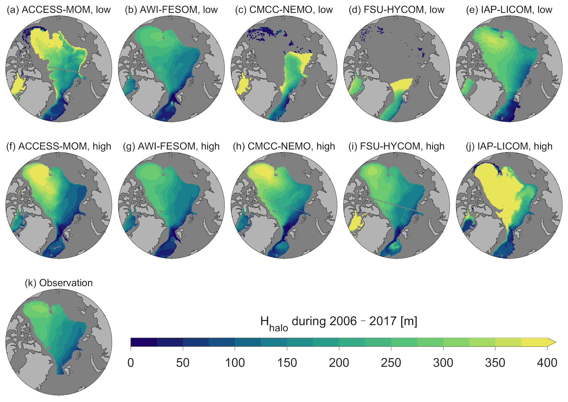
Figure 13Cold halocline base depth averaged over 2006–2017 in low-resolution (a–e) and high-resolution (f–j) models. We first calculated the cold halocline base depth in the deep-basin area (where the ocean bottom is deeper than 500 m) using monthly temperature and then averaged it over the considered period. If the depth cannot be found (because of the absence of Arctic Atlantic water warmer than 0 ∘C), this record was not taken into account during the average. A missing value indicates that the depth was not found throughout the considered period. The observational estimate is shown in (k) (Polyakov et al., 2020).
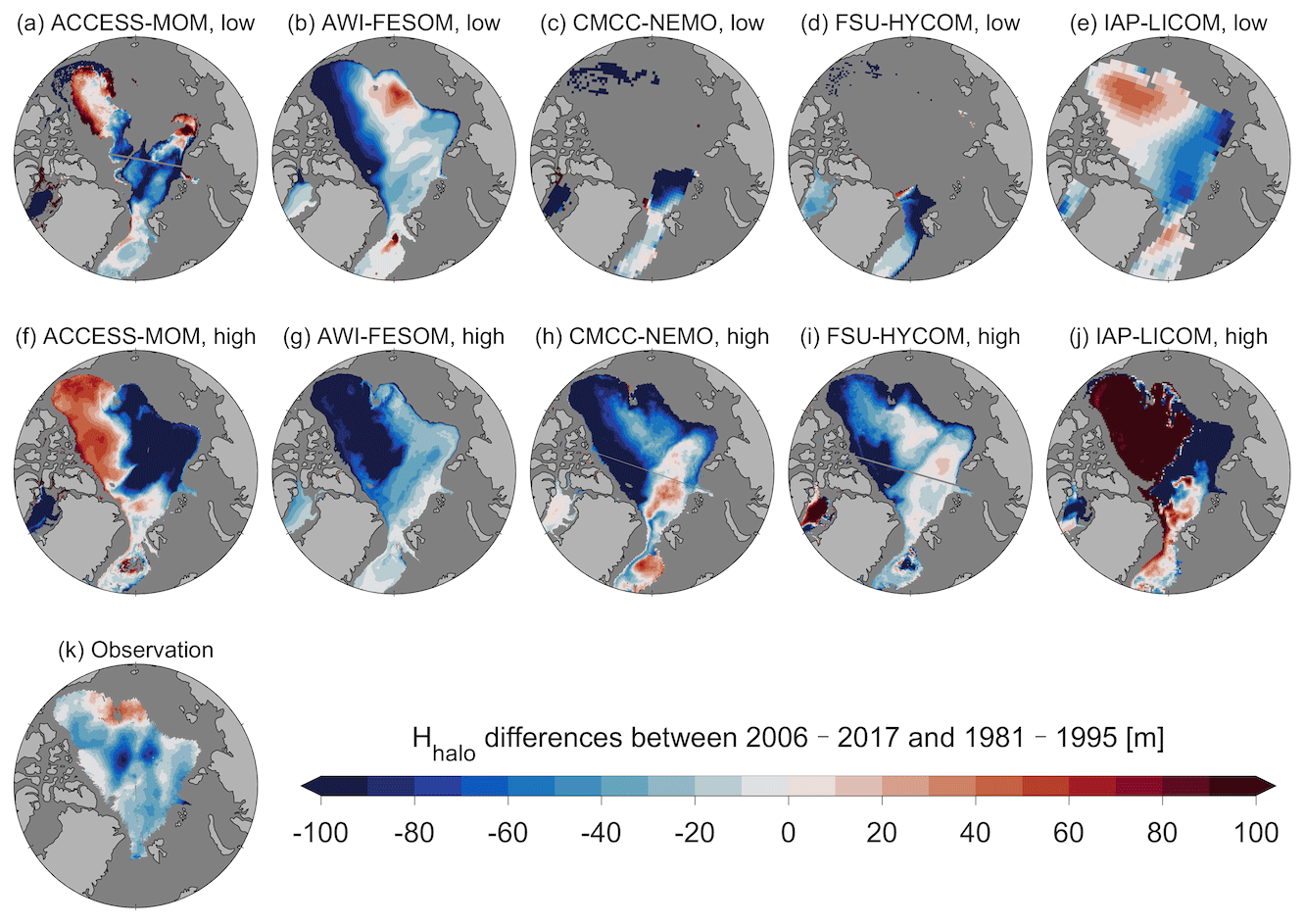
Figure 14Change in the cold halocline base depth between the period 2006–2017 and the period 1981–1995 in low-resolution (a–e) and high-resolution (f–j) models. The observational estimate (Polyakov et al., 2020) is shown in (k). A negative value indicates an uplift of the cold halocline base depth. The color in the Amerasian Basin in (j) is dark red.
Observations have shown a shoaling of the cold halocline base depth in most of the Arctic deep basin during the period 2006–2017 compared to 1981–1995 (Fig. 14k; Polyakov et al., 2020). However, the three models that show improvement in simulating the mean state of the cold halocline base depth with higher resolution (ACCESS-MOM, CMCC-NEMO and FSU-HYCOM) do not reproduce the observed shoaling in the Eurasian Basin or Canada Basin (Fig. 14f, h, i). Both configurations of the AWI-FESOM model simulate an uplift of the cold halocline base depth in the Eurasian Basin, with magnitudes similar to the observations (Fig. 14b, g). However, its high-resolution configuration exhibits a large overestimation of the uplift in the Canada Basin (Fig. 14g). The overestimation of the uplift in the Canada Basin is mainly due to the deep bias in the cold halocline base depth in the earlier period (1981–1995, Fig. S4) since the model reproduces the cold halocline base depth well in the recent period (2006–2017, Fig. 13g). The anomaly of the cold halocline base depth in the Amerasian Basin in IAP-LICOM is not consistent with the observations (Fig. 14j).
All the high-resolution models that can simulate the warming of the Atlantic water layer in the 2010s show an uplift of the cold halocline base depth in the Eurasian Basin within that decade (four out of five models, Fig. 10f–i). Thus, these models are able to reproduce the fact that the warm Atlantic water layer has become closer to the surface in the progression of Arctic Atlantification in the 2010s. However, in the high-resolution CMCC-NEMO, for the two periods that we compare here, the cold halocline base depth in the Eurasian Basin in 2006–2017 is slightly deeper than in 1981–1995 (Fig. 14h), contradicting the observations (Fig. 14k). The reason is that its cold halocline base depth is too shallow in the 1990s, associated with an overestimated warming event in that period (Fig. 10h).
3.4 Liquid freshwater content
The Arctic Ocean plays a crucial role in the hydrological cycle of the Northern Hemisphere (Carmack et al., 2016). It receives freshwater from various sources, including river runoff, net precipitation and low-salinity Pacific Water, while exporting freshwater to the subpolar North Atlantic. The Beaufort High, characterized by high sea level pressure, causes the freshwater in the Arctic to accumulate predominantly in the Canada Basin (McPhee et al., 2009; Proshutinsky et al., 2009, 2019; Timmermans and Marshall, 2020; Wang and Danilov, 2022). Due to the prevailing anticyclonic wind patterns over the Canada Basin and the decline in Arctic sea ice, the Arctic Ocean has been experiencing an increase in liquid freshwater content since the mid-1990s (Proshutinsky et al., 2019; Wang and Danilov, 2022). Observations have revealed that the amount of liquid freshwater in the Arctic basin in the mid-2010s was approximately 11 000 km3 more than in the mid-1990s (Rabe et al., 2014; Wang et al., 2019). The excess freshwater in the Arctic, when released into the convective regions of the North Atlantic, could impact deep-water formation and large-scale circulation (Aagaard et al., 1985; Goosse et al., 1997; Arzel et al., 2008). Therefore, assessing the Arctic freshwater content is important for understanding climate variability and change.
The freshwater content of the water column, referred to as the freshwater column in short (measured in meters), is defined as follows:
where S represents salinity, Sref is the reference salinity, and H is the depth at which the salinity equals the reference salinity. This quantifies the amount of pure water that needs to be removed from a column to change the mean salinity to the reference salinity. In this study, a reference salinity of Sref=34.8 psu, considered to be the mean salinity of the Arctic Ocean (Aagaard and Carmack, 1989), is used, consistently with previous studies (e.g., Serreze et al., 2006; Jahn et al., 2012; Haine et al., 2015; Wang et al., 2016a, 2023; Shu et al., 2023). The volumetric freshwater content is obtained by integrating the freshwater column over an area.
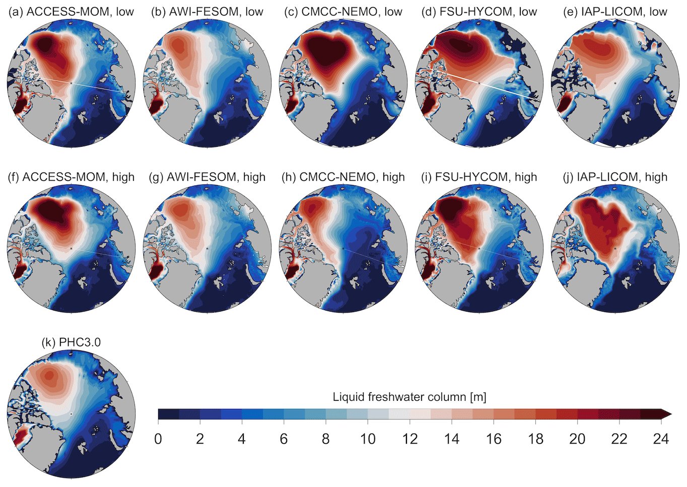
Figure 15Liquid freshwater column (in meters) averaged over 1971–2000 in (a–e) low-resolution and (f–j) high-resolution models. The estimate based on PHC3.0 (Steele et al., 2001) is shown in (k).
First, we evaluate the mean state of the simulated freshwater column (Fig. 15). The models generally capture the basic spatial pattern of the freshwater column, with higher values in the Canada Basin and lower values in the Eurasian Basin. However, there are notable differences in the spatial distribution and magnitudes of the freshwater column among the models. Two of the low-resolution models (CMCC-NEMO and FSU-HYCOM) tend to significantly overestimate the freshwater column in the Amerasian Basin (Fig. 15c, d), while one of them (AWI-FESOM) underestimates the freshwater column in the northwestern Amerasian Basin (Fig. 15b).
In the high-resolution models, ACCESS-MOM shows a stronger overestimation of the freshwater column in the Amerasian Basin compared to its low-resolution counterpart (Fig. 15a, f). AWI-FESOM remains largely similar between the two configurations (Fig. 15b, g), while CMCC-NEMO underestimates the freshwater column in the high-resolution configuration, contrarily to its overestimation in the low-resolution configuration (Fig. 15c, h). FSU-HYCOM displays an excessive concentration of freshwater in the southern Beaufort Sea in its high-resolution configuration (Fig. 15i), and IAP-LICOM fails to reproduce a realistic gyre shape in the Amerasian Basin's freshwater distribution (Fig. 15j). With the increase in model resolution, the consistency of the simulated freshwater column among the models is not clearly improved.
As the freshwater column plays a crucial role in determining the sea surface height and the surface geostrophic current in the Arctic basin (Armitage et al., 2017; Wang, 2021), the above results imply a large spread in the simulated ocean surface circulation among both low- and high-resolution models, as indicated by the spatial pattern of sea surface height (Fig. S5). With the increase in model resolution, the RMSE of Arctic sea surface height decreases in three models while increasing in two others.
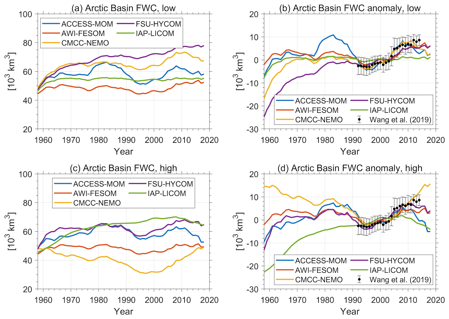
Figure 16(a) Time series of liquid freshwater content (FWC) in the Arctic basin in the low-resolution models. (b) The same as (a) but for the anomalies relative to the 1992–2008 mean. (c, d) The same as (a) and (b) but for the high-resolution models. The observational estimate (Wang et al., 2019) is shown in (b) and (d).
Next, we will assess the model spread in the Arctic basin freshwater content. Figure 16 presents the time series of freshwater content in the Arctic basin and their anomalies relative to the 1992–2008 mean. Consistently with the mean state of the freshwater column shown in Fig. 15, the model spread in simulating Arctic basin freshwater content remains similar in the high-resolution configurations in relation to the low-resolution configurations (Fig. 16a, c). In two low-resolution models (CMCC-NEMO and FSU-HYCOM), the freshwater content in the Arctic basin drifts upward over time (Fig. 16a). The most significant drift occurs during the first 10 years of the simulation, as also indicated in the time–depth plot of salinity (Fig. 9). In the high-resolution FSU-HYCOM model, the upward drift of total freshwater content is reduced (Fig. 16a, c), mainly attributed to the lower freshwater column outside the Beaufort Sea (Fig. 15d, i). The high-resolution CMCC-NEMO model simulates a downward drift in freshwater content during the first 40 years (Fig. 16c), which is associated with the evolution of positive salinity bias in the upper Amerasian Basin in terms of both magnitude and vertical extent (Fig. 9r). The high-resolution IAP-LICOM model, unlike its low-resolution counterpart, exhibits a strong upward drift (Fig. 16a, c).
Lastly, we will assess the simulation of temporal changes in the Arctic freshwater content. Except for IAP-LCOM, all models consistently simulate an increase in Arctic basin freshwater content during the observational period (Fig. 16b, d). In the low-resolution configurations, the simulated increase in freshwater content from the mid-1990s to the mid-2010s falls mostly within the uncertainty range of observational estimates (Fig. 16b). However, in the high-resolution configurations, the model–observation misfit becomes more pronounced in most models (Fig. 16d). The high-resolution CMCC-NEMO model shows a persistent increase in freshwater content from the mid-1990s until the end of the simulation, contrarily to observations indicating a leveling off in the mid-2010s (Wang et al., 2019). In contrast to high-resolution CMCC-NEMO, both high-resolution ACCESS-MOM and IAP-LICOM models simulate a declining trend starting from the early 2010s, which differs from the observed leveling off in the mid-2010s. Only AWI-FESOM and FSU-HYCOM reproduce the leveling off of freshwater content in the mid-2010s in the high-resolution models. FSU-HYCOM performs the best in simulating the temporal changes in freshwater content, as both of its configurations produce freshwater content anomalies that fall within the observational uncertainty range.
Several factors can influence Arctic freshwater content, such as winds, sea ice effects on momentum transfer, and the surface geostrophic currents which influence the circulation pathway and residence time of freshwater in the Arctic Ocean (Wang et al., 2021). The two models that show the greatest deterioration in simulating freshwater content changes in their high-resolution configurations compared to their low-resolution configurations, ACCESS-MOM and CMCC-NEMO, exhibit the largest biases in surface salinity among the models (Fig. 7). ACCESS-MOM has limited sea surface salinity restoring, and it is switched off under sea ice in CMCC-NEMO. These findings suggest that model resolution is not the dominant factor influencing the model's performance in simulating the mean state of freshwater spatial distribution and the temporal changes in Arctic freshwater content. The models tend to need sea surface salinity restoring to climatology to avoid large salinity biases at the surface.
3.5 Gateway transports
Arctic climate is strongly influenced by inflows from the Atlantic and Pacific oceans. As mentioned in Sect. 3.4, the transport of ocean heat from lower latitudes significantly affects the temperature of the Arctic Ocean (Polyakov et al., 2020; Shu et al., 2022), the extent of Arctic sea ice in the cold season (Woodgate et al., 2010; Årthun et al., 2012, 2019; Shu et al., 2021; Yamagami et al., 2022; Pan et al., 2023) and winter air temperature (Screen and Simmonds, 2010; Årthun et al., 2017; Nummelin et al., 2017). The Arctic Ocean also exports freshwater to the subpolar North Atlantic, with potential impacts on upper-ocean stratification, deep-water formation, large-scale circulation and climate dynamics (Aagaard et al., 1985; Goosse et al., 1997; Arzel et al., 2008). Furthermore, the inflows and outflows through the Arctic Ocean gateways play a crucial role in the transport of nutrients and planktonic organisms (Walsh et al., 1989; Hátún et al., 2017; Basedow et al., 2018; Ingvaldsen et al., 2021). Observations and model simulations consistently indicate that ocean heat convergence to the Arctic Ocean and the hydrological cycle in the Arctic region are intensifying under a warming climate (Wang et al., 2023). In this subsection, we will assess the models' ability to simulate the mean state and temporal changes in Arctic–Subarctic ocean transports through key gateways (the Bering Strait, Barents Sea Opening, Fram Strait and Davis Strait; see Fig. 1).
The ocean volume (VT), heat (HT) and freshwater (FWT) transports through a gateway transect are defined as follows:
where un represents the ocean velocity perpendicular to the transect, θ denotes potential temperature, θref is the reference temperature, S indicates salinity, Sref is the reference salinity, ρo corresponds to ocean density, cp represents the specific heat capacity of seawater, and the integration is performed over the height z from the ocean bottom to the surface and over the distance ℓ along the transect. Ocean heat transports are calculated relative to θref=0 ∘C, and freshwater transports are calculated relative to Sref=34.8 psu, which is an estimate of the mean salinity of the Arctic Ocean (Aagaard and Carmack, 1989).
Monthly velocity, temperature and salinity data are available from the model outputs and are used in the calculations so eddy transports are largely neglected. It was suggested that heat directly transported by eddies is small at the Fram Strait (Kawasaki and Hasumi, 2016), while eddies can influence the mean flow into the Arctic basin by altering the distribution of the Atlantic water current between the re-circulation branch and the inflow branch (Wekerle et al., 2017; Hattermann et al., 2016). Additionally, it should be noted that mooring instruments used for measuring ocean transports have low spatial resolutions without covering whole gateway transects, and as a result, the uncertainties associated with transport estimates are usually large (e.g., Beszczynska-Moeller et al., 2011; Wang et al., 2023). Nonetheless, despite these limitations, these estimates represent the most reliable data currently available for evaluating models.
3.5.1 Bering Strait
The Bering Strait volume transport had a climatological value of 0.8±0.2 Sv, but it increased to 1±0.1 Sv in the last 2 decades (Woodgate and Peralta-Ferriz, 2021). Both the ocean heat and freshwater transports also increased during this period, from 4 TW and 2400±300 km3 yr−1 in 1980–2000 to 6 TW and 3000±280 km3 yr−1 in 2000–2020 (Woodgate and Peralta-Ferriz, 2021; Wang et al., 2023). The low- and high-resolution models exhibit similar spreads in the Bering Strait volume, heat and freshwater transports (Fig. 17). Despite the model spreads, the interannual variability of the Bering Strait transports is highly consistent among the models regardless of model resolution (Fig. S6), as found in previous model intercomparisons (Wang et al., 2016a; Shu et al., 2023).
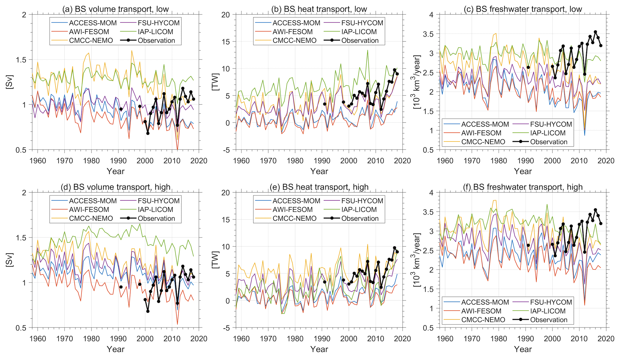
Figure 17Time series of ocean (a) volume, (b) heat and (c) freshwater transports in the Bering Strait (BS) in low-resolution models. (d, e, f) The same as (a), (b) and (c) but for high-resolution models. Heat transport is referenced to 0 ∘C, and freshwater transport is referenced to 34.8 psu. The observational estimates are adopted from Woodgate and Peralta-Ferriz (2021).
It has been found that low-resolution ocean models struggle to reproduce the observed upward trend in Bering Strait volume transport (Shu et al., 2023). Increasing the resolution does not improve this issue in any of the models analyzed in our study (Fig. 17a, d). As these models employ various numerical methods, resolutions, and parameterizations, but still exhibit the same issue, it is likely that the problem originates from the atmospheric reanalysis and runoff data (JRA55-do) used to drive these models. The models are able to capture the observed increase in heat transport over the past decade (Fig. 17b, e), indicating that the warming of the Pacific Water inflow contributes partially to the increase in ocean heat transport (Woodgate and Peralta-Ferriz, 2021; Wang et al., 2023). However, none of the models simulate the observed increase in freshwater transport (Fig. 17c, f) because the rise in freshwater transport is primarily driven by the increase in volume transport (Woodgate and Peralta-Ferriz, 2021). Overall, for the Bering Strait, both the model spreads and the models' abilities to simulate interannual variability and decadal trends are not substantially influenced by model resolution.
3.5.2 Barents Sea Opening
The ocean volume transport through the Barents Sea Opening did not show a statistically significant trend over the past few decades, but the ocean heat transport exhibited an upward trend (Skagseth et al., 2020). Based on mooring observations in the 1990s and 2000s, the climatology of ocean volume transport is estimated to be between 2 and 2.3 Sv (Smedsrud et al., 2010, 2013). The models tend to overestimate the volume transport in both their low-resolution and high-resolution configurations (Fig. 18a, d). The low-resolution CMCC-NEMO model stands out as an outlier, with a volume transport nearly twice that of the observations, while this bias is reduced in its high-resolution counterpart. The heat transport in the Barents Sea Opening was approximately 70 TW in the 2000s (Smedsrud et al., 2013). Two low-resolution models, FSU-HYCOM and IAP-LICOM, underestimate the heat transport, while their high-resolution counterparts exhibit higher heat transport, becoming similar to (IAP-LICOM) or even larger (FSU-HYCOM) than the observations (Fig. 18b, e). Although increasing the horizontal resolution improves the ocean volume transport in CMCC-NEMO, the high-resolution model still exhibits a positive bias in heat transport, indicating the influence of warmer ocean temperatures. Nevertheless, the model spreads in the Barents Sea Opening volume and heat transports are slightly reduced in the high-resolution models (Fig. 18a, b, d, e), suggesting potential model improvements with increasing resolution.
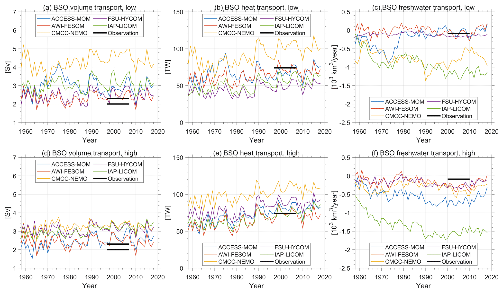
Figure 18The same as Fig. 17 but for the Barents Sea Opening (BSO). The observational estimates are taken from Smedsrud et al. (2013) and Serreze et al. (2006).
The interannual variability of ocean volume and heat transports is consistent among the models and is not strongly influenced by model resolution (Fig. S7). A synthesis of models and observations suggests an increase in heat transport of approximately 8 TW from 1980–2000 to 2000–2020 (Wang et al., 2023). The models simulate a consistent trend, with an increase close to this value.
The Atlantic water inflow in the Barents Sea Opening is saltier than the average salinity of the Arctic Ocean, making it a freshwater sink for the Arctic Ocean. The net freshwater transport in the Barents Sea Opening is a small, negative value, estimated to be around −100 km3 yr−1 (Serreze et al., 2006). In both the low-resolution and high-resolution models, there are two models that simulate excessively large negative values (Fig. 18c, f). IAP-LICOM exhibits the largest biases in both groups. As it does not have outlier volume transports, the biases in freshwater transport are primarily due to its positive salinity biases in the inflow. The interannual variability of freshwater transport is not consistent among the low-resolution models but improves in the high-resolution models (Fig. S7).
3.5.3 Fram Strait
The climatological net volume transport through the Fram Strait is estimated to be Sv (Schauer et al., 2008). Among the low-resolution configurations, two models (AWI-FESOM and FSU-HYCOM) exhibit a good representation of the mean volume transport, while four of the high-resolution configurations perform well, except for CMCC-NEMO (Fig. 19a, d). The mean heat transport through the Fram Strait was approximately 30 TW in the period 1980–2000 and increased to about 40 TW in 2000–2020 (Wang et al., 2023). Three of the low-resolution configurations (CMCC-NEMO, FSU-HYCOM and IAP-LICOM) show insufficient heat transport (Fig. 19b), which contributes to their strong cold biases in the Atlantic water layer (Figs. 4 and 5). In all the models, the heat transport increases with resolution (Fig. 19b, e), with the weakest increase observed in AWI-FESOM, possibly due to there being the same model resolution outside the Arctic Ocean in both configurations. Two models (CMCC-NEMO and FSU-HYCOM) exhibit excessively high heat transport in their high-resolution configurations, contributing to the excessively warm Atlantic water layer in these models (Fig. 6h, i). The climatological freshwater transport in the Fram Strait is approximately km3 yr−1 (Serreze et al., 2006). Two low-resolution models (CMCC-NEMO and ACCESS-MOM) either significantly underestimate or overestimate the freshwater transport in the Fram Strait (Fig. 19c). The model spread in the Fram Strait freshwater transport is considerably reduced in the high-resolution models (Fig. 19f).
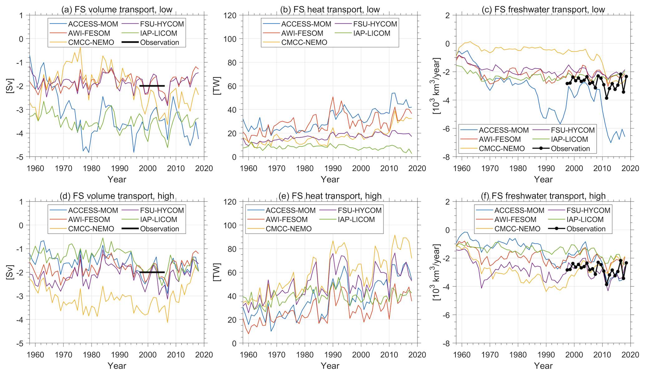
Figure 19The same as Fig. 17 but for the Fram Strait (FS). The observational estimates are taken from Schauer et al. (2004) and Karpouzoglou et al. (2022).
Most of the low-resolution models tend to exhibit weak interannual variability in the Fram Strait heat and freshwater transports (Figs. 19 and S8). With the exception of IAP-LICOM, all the high-resolution models simulate an increase in heat transport in the early 1990s and the first 2 decades of the 21st century, consistently with the changes suggested by observations and previous model studies (Polyakov et al., 2013; Wang et al., 2020b). On the contrary, these decadal changes in ocean heat transports are not captured by three of the low-resolution models. Observations indicate an increase in freshwater export in 2010–2013 compared to the 2000s, as manifested by strengthened currents and lower salinity (de Steur et al., 2018). All the high-resolution models simulate an increase in freshwater export over this period, with two models (AWI-FESOM and FSU-HYCOM) even capturing a magnitude similar to the observed increase (Fig. 19f). In contrast, all the low-resolution models exhibit either an overestimation or underestimation of the magnitude of this freshwater transport change (Fig. 19c). Therefore, the simulated variability of ocean heat and freshwater transports in the Fram Strait is notably improved with increasing resolution.
3.5.4 Davis Strait
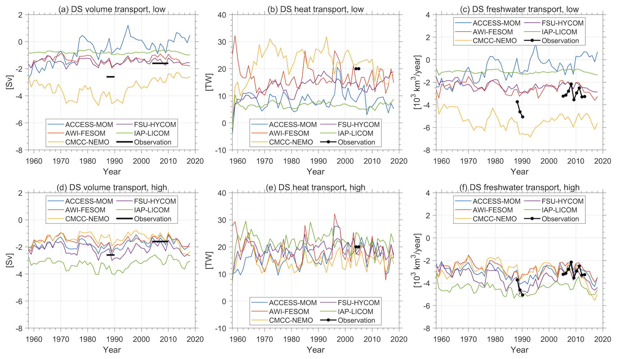
Figure 20The same as Fig. 17 but for the Davis Strait (DS). The observational estimates are taken from Cuny et al. (2005) and Curry et al. (2014).
The volume transport in the Davis Strait was estimated to be Sv in 1987–1990 (Cuny et al., 2005) and Sv in 2004–2010 (Curry et al., 2014). Among the low-resolution models, IAP-LICOM exhibits a low volume export without clear interannual variability (Fig. 20a) due to the closure of the western straits in the Canadian Arctic Archipelago (Fig. 2e). The low-resolution ACCESS-MOM model shows unrealistically positive volume transport (inflow to the Arctic) in some years. In both low-resolution IAP-LICOM and ACCESS-MOM models, the biases in volume transport in the Davis Strait are anticorrelated with the biases in the Fram Strait (Figs. 19a and 20a) because the Arctic export is distributed between these two gateways (Wang et al., 2023). The low-resolution CMCC-NEMO model exhibits excessively high volume export, nearly double the observed values. The model spread in the mean volume transport is significantly reduced in the high-resolution models (Fig. 20d). The climatological heat and freshwater transports in Davis Strait are estimated to be 18±17 TW and km3 yr−1, respectively, based on observations at the end of the 1980s (Cuny et al., 2005). Similarly to the biases in volume transport, the heat and freshwater transports in the Davis Strait are either too low or too high in the three aforementioned low-resolution models (Fig. 20b, c). Increasing resolution reduces the model spread and brings the results closer to the observations for both heat and freshwater transports (Fig. 20e, f). It is important to acknowledge that the observation of the Davis Strait heat transport has a very limited time span and is accompanied by substantial uncertainty. However, irrespective of this limitation, a decrease in model spread suggests improvements in high-resolution models.
Increasing resolution clearly improves the intermodel consistency in the simulated interannual variability of ocean volume and freshwater transports in the Davis Strait, but this is not the case for heat transport (Fig. S9). This indicates that the models exhibit less agreement in simulating the advection of water of Atlantic origin from the Irminger Sea to Baffin Bay. The high-resolution models consistently simulate a reduction in the Davis Strait volume and freshwater exports in the early 1990s and an increase in the middle to late 2010s. The former reduction is primarily due to the positive Arctic Oscillation, which shifted more Arctic export to the Fram Strait, while the latter increase is mainly attributed to the drop in dynamic sea level south of Greenland (Q. Wang et al., 2022; Wang et al., 2023). The increase in the Davis Strait freshwater export from 2010 to 2017 exceeded 1500 km3 yr−1, as suggested in a previous modeling study (Q. Wang et al., 2022). This magnitude of increase is quantitatively reproduced in all the high-resolution models except for CMCC-NEMO, which simulates a too-large increase.
4.1 Model spin-up and integration length
There is no consensus about how to initialize sea ice models at the beginning of simulations in the OMIP-2 protocol, and practically different modeling groups used different data sets of temperature and salinity climatology to initialize their ocean models (Chassignet et al., 2020). As shown in Fig. 9, in models with large salinity biases relative to climatology, their salinity drifts away from initial conditions quickly within the first few model years. The time series of freshwater content further demonstrate that (i) the model spread is relatively small in the first year, and (ii) it increases quickly with time within the first few years (Fig. 16). This indicates that our model intercomparison is not significantly influenced by differences in model initial conditions. The depth–time plots of basin temperature show that the temperature differences between models also stem mainly from model drift and not initial conditions (Fig. 10).
In this study, our primary focus was on the first cycle of the OMIP-2 simulations due to limitations in model data availability. The simulated ocean, especially the deep ocean, does not reach a quasi-equilibrium state within this integration length. For one of the participating models, ACCESS-MOM, we had access to data for a few cycles. We compared temperature profiles for the last year (2018) of the first three simulation cycles from this model (see Fig. S10). We found that, in the low-resolution configuration, the vertical temperature profiles continue to homogenize over time, whereas, in the high-resolution configuration, temperature has a smaller drift over time. This finding reinforces the advantages of utilizing a high resolution.
4.2 Representativeness of analyzed models
Despite the fact that we have a relatively small group of model pairs in this study, the models show the common issues identified in previous model intercomparison studies, thus allowing us to investigate the impacts of model resolutions on these issues. However, quantitatively, the multi-model mean of these models may not be able to represent the situation where all ocean models used in CMIP simulations are considered. For example, there are models with overly warm Barents–Kara seas and an overly warm Arctic basin, as identified in previous CORE-II and CMIP model intercomparison studies (Ilicak et al., 2016; Shu et al., 2019), while there are no models of this kind in our small model set.
The employed model resolutions are determined by each modeling group according to their model development strategy, experience and available computing resources and are not specified in the OMIP-2 protocol. This is in line with how CMIP models are developed. As a result, the model resolutions differ notably in both the low- and high-resolution sets. The comparison between the two model sets reflects possible changes between models in the phase of CMIP6 and future CMIP phases. Despite the variety in the resolutions between the models, the improvements in simulating Arctic temperature and salinity by means of increased resolutions are consistent among the models, except for one model that used a sea ice model without dynamics in its high-resolution version.
The low-resolution AWI-FESOM model exhibits more realistic hydrography and stratification than some of the high-resolution models. Therefore, in future ocean model developments for improving Arctic Ocean simulations, tuning model parameterizations and/or some numerical aspects is just as crucial as increasing model resolution. One of the possible reasons that AWI-FESOM has relatively small temperature biases in the Arctic basin could be that it reasonably simulates the temperature in the Barents–Kara seas (see more discussions in Sect. 4.4).
4.3 Horizontal resolution versus vertical resolution
Two of the models included in this study allow us to clearly distinguish the impacts of horizontal resolution from those of vertical resolution. In FSU-HYCOM, the high-resolution configuration has a coarser vertical resolution compared to the low-resolution configuration. Therefore, the improved simulation of Atlantic water layer temperature, halocline salinity and some gateway transports in the high-resolution FSU-HYCOM can be mainly attributed to increased horizontal resolution.
In AWI-FESOM, the vertical resolution remains the same in both configurations. The reduced thickness of the Atlantic water layer and the improved cyclonic circulation of the Atlantic water in the deep basin in the high-resolution configuration are therefore associated with increased horizontal resolution. Among the five model pairs, AWI-FESOM exhibits the smallest difference between the two configurations. Firstly, its low-resolution configuration does not exhibit extreme biases, leaving less room for improvement. Secondly, the resolution outside the Arctic is the same in both AWI-FESOM configurations, indicating that the difference in simulation results is solely due to the local differences in model configurations. In other models, the impacts of different resolutions outside the Arctic can propagate into the Arctic Ocean through gateway transports, contributing to the Arctic differences within the model pairs.
4.4 Processes related to temperature and salinity biases
Our model intercomparison offers some clues for model developers and users with regard to improving certain processes in their models. For instance, the low-resolution ACCESS-MOM model (with a horizontal resolution of about 9 km, higher than in the other low-resolution models) exhibits the highest net heat transport through the Fram Strait among the low-resolution models, but it has a significant cold bias in the Arctic basin. This suggests that the cold water originating from the Barents Sea is the main cause of the basin's cold bias in this model. The other two low-resolution models (CMCC-NEMO and FSU-HYCOM) with cold biases in the Arctic basin also simulate excessively cold water in the northeast Barents Sea. In the high-resolution configurations of these models, the cold biases in the northeast Barents Sea are largely eliminated. However, as the other two low-resolution models (AWI-FESOM and IAP-LICOM) do not exhibit significant cold biases in the northeast Barents Sea, it is possible that a low resolution alone is not the primary cause of the cold biases. Previous analyses of forced ocean–ice models (Ilicak et al., 2016) and coupled climate models (Shu et al., 2019) have actually shown that some models could have too-warm water originating from the Barents Sea. It was also found that the temperature biases in the Arctic basin are significantly correlated with ocean temperature and winter mixed-layer depth in the Barents–Kara seas (Shu et al., 2019). Therefore, investigating the air–sea heat exchange and water mass transformation in the Barents–Kara seas in models exhibiting strong cold or warm biases may offer insights into effectively reducing Arctic Ocean temperature biases in low-resolution models. The fact that increasing resolution does help reduce cold biases in the northeast Barents Sea in our analyzed models implies that some resolution-dependent parameterizations or numerics in these models may contribute to the biases.
In terms of the model representation of Arctic freshwater, particularly regarding the spatial distribution and temporal changes in freshwater content, notable improvement is not observed with increasing resolution. Although salinity biases in the halocline are reduced in some high-resolution configurations, two models exhibit similar or even larger sea surface salinity biases when their spatial resolution is improved. This could potentially be attributed to weak or absent sea surface salinity restoration. The strong dependence of simulated sea surface salinity on numerical restoration indicates the general need for improvements in the surface freshwater budget and the processes influencing freshwater circulation and distribution, such as the impact of sea ice on momentum transfer in models. Reducing the overall biases in salinity, which remain large in most of the high-resolution models, is crucial as the surface geostrophic currents in the Arctic basin are directly influenced by the spatial pattern of the freshwater column (Armitage et al., 2017; Wang, 2021).
4.5 Comments on impacts of mesoscale eddies
Assessing mesoscale eddy activity in the high-resolution simulations is beyond the scope of this paper. It is worth noting that the high-resolution OMIP-2 models assessed in this study only marginally permit mesoscale eddies in the Arctic Ocean. The influence of eddies appears to be reflected in the disparity in winter MLDs between two configurations for some of the models. However, there is no conclusive evidence suggesting that the major improvements in the high-resolution models are attributable to simulated eddies in the Arctic Ocean. In particular, the first baroclinic Rossby radius in the Barents Sea is extremely small (approximately 2 km; Nurser and Bacon, 2014), and these high-resolution models cannot adequately resolve eddies in this region. Therefore, the reduction in the large temperature bias in the northeastern Barents Sea (and thus in the Arctic deep basin) in three of the analyzed models cannot be attributed to resolved eddies in the Barents Sea. Moreover, despite the fact that eddy transport was proposed to be one of the key factors influencing the amount of freshwater in the Beaufort Gyre (Manucharyan and Spall, 2016; Meneghello et al., 2017), we did not observe notable improvements in the simulated mean state or variability of the Arctic freshwater content in the investigated high-resolution models.
Mesoscale eddies can influence the distribution of warm Atlantic water between the inflow to the Arctic basin and the recirculation branch in the Fram Strait (Hattermann et al., 2016; Wekerle et al., 2017). Some permitted eddies in the high-resolution models could contribute to the improvement in ocean heat inflow in the Fram Strait in terms of mean state and variability. However, it has been suggested that 1 km resolution is needed to simulate well the mesoscale eddies in the Fram Strait and, thus, capture their effect (Wekerle et al., 2017). Therefore, it is likely that other factors, such as the reduction in numerical mixing and the improved representation of topographic steering of ocean currents at higher resolutions, played a more important role in altering the distribution of Atlantic water between its two branches and improving the inflow in the Fram Strait.
This paper assesses Arctic Ocean simulations using five pairs of matched low- and high-resolution models within the CMIP6 OMIP-2 framework (Griffies et al., 2016). The primary objective is to investigate whether increasing resolution can mitigate the typical model biases in low-resolution models identified in previous studies, which have persisted for more than 2 decades. The main findings are summarized below.
-
The low-resolution models exhibit warm biases below the core depth range of the Atlantic water layer, even when cold biases are present in the Atlantic water layer. This reflects the common issue of the Atlantic water layer being excessively thick in low-resolution models. Additionally, the halocline and upper Atlantic water layer exhibit fresh biases in low-resolution models. These issues have been linked to spurious vertical mixing (Holloway et al., 2007; Wang et al., 2016a). Increasing resolution alleviates these issues in some model pairs but not in all cases, implying that other factors, such as differences in parameterizations and simulated sea ice dynamics, could also influence the comparison.
-
An increase in horizontal resolution helps reduce biases in mean temperature and salinity in four of the five models. By increasing resolution, the RMSE of basin temperature in the upper 3500 m is reduced by 17 % and 33 % in the Eurasian Basin and Amerasian Basin, respectively, when averaged over the five models. The multi-model-mean improvement in salinity is less prominent, with a reduction in RMSE of 8 % in the upper 700 m of the Amerasian Basin and no reduction in Eurasian Basin.
-
Three of the low-resolution configurations display significant cold biases in the Atlantic water layer, which can be attributed to insufficient warm Atlantic water inflow in the Fram Strait and excessive cold water originating from the Barents Sea, similarly to what was found in previous analyses of low-resolution models (Ilicak et al., 2016; Shu et al., 2023). A higher resolution reduces the temperature biases in all these models by enhancing the Fram Strait heat import and reducing the cold bias in the northeastern Barents Sea. By increasing the resolution, the RMSE of temperature at 400 m depth is reduced by 39 % when averaged over the five models. The RMSE of salinity at 400 m depth is also reduced by 13 %.
-
Decadal warming events in the Atlantic water layer are better simulated with a higher resolution. While only one low-resolution model adequately reproduces the warming of the Atlantic water layer in the 1990s and 2010s, four high-resolution models can do so. These warming events arise from episodes of intensified heat flux through the Fram Strait, which are more accurately represented in high-resolution models. Observations show that the Atlantic water core temperature increased by 0.3 ∘C in the period of 2006–2017 compared to the period of 1981–1995. On average, the five low-resolution models underestimated this warming by 58 %, while the five high-resolution models overestimated this warming by a smaller percentage of 23 %.
-
High-resolution models exhibit shallower surface MLDs, possibly reflecting the influence of permitted but not well-resolved eddies in restratifying the mixed layer. Two low-resolution models significantly overestimate the MLD, but this bias is reduced in their high-resolution counterparts in parts of the Arctic basin. However, the reduction in the MLD bias is not accompanied by a reduction in salinity bias. Among the models capable of reasonably simulating the warm Atlantic water layer (one low-resolution model and four high-resolution models), the shoaling trend of the cold halocline base depth in the eastern Eurasian Basin during the 2010s is captured. However, the high-resolution models do not consistently simulate changes in the cold halocline base depth on multi-decadal timescales.
-
Model performance in simulating the mean state of freshwater spatial distribution and the temporal changes in Arctic freshwater content does not improve with a higher resolution. Although the bias in halocline salinity is reduced in high-resolution models, the sea surface salinity bias could worsen depending on the approach used for sea surface salinity restoring. This factor appears to have a non-negligible impact on the model's representation of Arctic freshwater content and, thus, on the simulated sea surface height.
-
An increase in horizontal resolution improves the simulation of Arctic gateway transports, primarily for the Fram and Davis straits. For these two gateways, high-resolution models exhibit reduced spreads in the transports, closer agreement with observations regarding the mean states, and improved quantitative representation of variability and changes. Models agree more on the temporal variability than the mean state of the gateway transports, as found in previous model intercomparison studies (Wang et al., 2016a; Shu et al., 2023). Increasing resolution does not resolve the challenge of simulating the observed increase in Pacific water inflow in the 2010s, suggesting that the origin of this issue may lie in the common atmospheric and runoff forcing.
Overall, we found that increasing resolution has the potential to improve model representation of the Arctic Ocean, including temperature and salinity in the Arctic basin, Atlantic water layer, mixed-layer depth, cold halocline base depth, and ocean transports through the Fram and Davis straits, although not all models achieve improvements for all these variables.
It is unlikely that most climate models participating in near-future CMIP7 deck and scenario simulations will have resolutions higher than those employed in the current high-resolution OMIP-2 models. Therefore, our evaluation of the OMIP-2 models provides valuable and timely information for groups preparing future CMIP simulations. In particular, we suggest that some of the extreme model biases are not primarily due to a low resolution alone, and investigating model numerics and parameterizations could help improve the representation of the Arctic Ocean in medium-resolution models used in climate-scale simulations.
The following OMIP model outputs, published on the Earth System Grid Federation, have been used: ACCESS-MOM (ACCESS-OM2) (https://doi.org/10.22033/ESGF/CMIP6.14690, Holmes et al., 2021), CMCC-NEMO (CMCC-CM2-SR5) (https://doi.org/10.22033/ESGF/CMIP6.13236, Fogli et al., 2020) and IAP-LICOM (FGOALS-f3-H and FGOALS-f3-L) (https://doi.org/10.22033/ESGF/CMIP6.3413, Lin, 2019; https://doi.org/10.22033/ESGF/CMIP6.13283, Lin, 2020). The ∘ ACCESS-MOM data are available from https://doi.org/10.25914/608097cb3433f (Kiss et al., 2020). The model data used to produce the figures and the corresponding analysis scripts are archived at https://doi.org/10.5281/zenodo.8046638 (Shu, 2023).
The supplement related to this article is available online at: https://doi.org/10.5194/gmd-17-347-2024-supplement.
QW coordinated the conceptualization and wrote the first draft of the paper. QS and SW processed the model data and produced the figures. QW, AB, EPC, PGF, AMH, DI, AEK, NK, YL, PL, HL, PS, DS and XX provided model data sets and expertise for the interpretation of the results. IP provided the gridded AWCT and halocline observational data. All the authors contributed to the interpretation of the results, the discussion of the scientific content and improvement of the paper.
At least one of the (co-)authors is a member of the editorial board of Geoscientific Model Development. The peer-review process was guided by an independent editor, and the authors also have no other competing interests to declare.
Publisher's note: Copernicus Publications remains neutral with regard to jurisdictional claims made in the text, published maps, institutional affiliations, or any other geographical representation in this paper. While Copernicus Publications makes every effort to include appropriate place names, the final responsibility lies with the authors.
We thank the present and past members of the CLIVAR Ocean Model Development Panel who have designed and supported the Ocean Model Intercomparison Project (OMIP). Qiang Wang is supported by the Helmholtz Climate Initiative REKLIM (Regional Climate Change and Human) and the EPICA project under the research theme “MARE:N – Polarforschung/MOSAiC”, funded by the German Federal Ministry for Education and Research with grant no. 03F0889A. Qi Shu is supported by the National Natural Science Foundation of China (grant no. 42276253), the Shandong Provincial Natural Science Foundation (grant no. ZR2022JQ17) and the Taishan Scholars Program (grant no. tsqn202211264). Andrew E. Kiss is supported by ARC grant no. LP200100406. Baylor Fox-Kemper is supported by the SASIP project of the Schmidt Futures Foundation. The ACCESS-MOM model runs were undertaken with the assistance of resources from the National Computational Infrastructure (NCI) and the Consortium for Ocean-Sea Ice Modelling in Australia, which are supported by the Australian Government. Nikolay Koldunov and Patrick Scholz are supported by S1: Diagnosis and Metrics in Climate Models and S2: Improved parameterisations and numerics in climate models of the Collaborative Research Centre TRR 181 “Energy Transfer in Atmosphere and Ocean”, funded by the Deutsche Forschungsgemeinschaft (DFG, German Research Foundation, project no. 274762653)
This research has been supported by the Bundesministerium für Bildung und Forschung (grant no. 03F0889A) and the National Natural Science Foundation of China (grant no. 42276253), the Shandong Provincial Natural Science Foundation (grant no. ZR2022JQ17), the Taishan Scholars Program (grant no. tsqn202211264), Australian Research Council (grant no. LP200100406), the SASIP project of the Schmidt Futures Foundation, and the Deutsche Forschungsgemeinschaft (DFG, German Research Foundation, project no. 274762653).
The article processing charges for this open-access publication were covered by the Alfred-Wegener-Institut Helmholtz-Zentrum für Polar- und Meeresforschung.
This paper was edited by Riccardo Farneti and reviewed by two anonymous referees.
Aagaard, K. and Carmack, E. C.: The Role Of Sea Ice And Other Fresh-Water In The Arctic Circulation, J. Geophys. Res., 94, 14485–14498, 1989. a, b
Aagaard, K., Swift, J. H., and Carmack, E.: Thermohaline Circulation In the Arctic Mediterranean Seas, J. Geophys. Res.-Oceans, 90, 4833–4846, 1985. a, b
Aksenov, Y., Karcher, M., Proshutinsky, A., Gerdes, R., de Cuevas, B., Golubeva, E., Kauker, F., Nguyen, A. T., Platov, G. A., Wadley, M., Watanabe, E., Coward, A. C., and Nurser, A. J. G.: Arctic pathways of Pacific Water: Arctic Ocean Model Intercomparison experiments, J. Geophys. Res.-Oceans, 121, 27–59, 2016. a
Allende, S., Fichefet, T., Goosse, H., and Treguier, A. M.: On the ability of OMIP models to simulate the ocean mixed layer depth and its seasonal cycle in the Arctic Ocean, Ocean Model., 184, 102226, https://doi.org/10.1016/j.ocemod.2023.102226, 2023. a
Armitage, T. W. K., Bacon, S., Ridout, A. L., Petty, A. A., Wolbach, S., and Tsamados, M.: Arctic Ocean surface geostrophic circulation 2003–2014, The Cryosphere, 11, 1767–1780, https://doi.org/10.5194/tc-11-1767-2017, 2017. a, b
Årthun, M., Eldevik, T., Viste, E., Drange, H., Furevik, T., Johnson, H. L., and Keenlyside, N. S.: Skillful prediction of northern climate provided by the ocean, Nat. Commun., 8, 15875, https://doi.org/10.1038/ncomms15875, 2017. a
Årthun, M., Eldevik, T., and Smedsrud, L. H.: The Role of Atlantic Heat Transport in Future Arctic Winter Sea Ice Loss, J. Climate, 32, 3327–3341, 2019. a
Arzel, O., Fichefet, T., Goosse, H., and Dufresne, J.-L.: Causes and impacts of changes in the Arctic freshwater budget during the 20th and 21st centuries in an AOGCM, Clim. Dynam., 30, 37–58, 2008. a, b
Bao, Q., Lin, P., Zhou, T., Liu, Y., Yu, Y., Wu, G., He, B., He, J., Li, L., Li, J., Li, Y., Liu, H., Qiao, F., Song, Z., Wang, B., Wang, J., Wang, P., Wang, X., Wang, Z., Wu, B., Wu, T., Xu, Y., Yu, H., Zhao, W., Zheng, W., and Zhou, L.: The Flexible Global Ocean-Atmosphere-Land system model, Spectral Version 2: FGOALS-s2, Adv. Atmos. Sci., 30, 561–576, https://doi.org/10.1007/s00376-012-2113-9, 2013. a
Basedow, S. L., Sundfjord, A., von Appen, W.-J., Halvorsen, E., Kwasniewski, S., and Reigstad, M.: Seasonal Variation in Transport of Zooplankton Into the Arctic Basin Through the Atlantic Gateway, Fram Strait, Front. Mar. Sci., 5, 194, https://doi.org/10.3389/fmars.2018.00194, 2018. a
Beszczynska-Moeller, A., Woodgate, R. A., Lee, C., Melling, H., and Karcher, M.: A Synthesis of Exchanges Through the Main Oceanic Gateways to the Arctic Ocean, Oceanography, 24, 82–99, 2011. a
Beszczynska-Moeller, A., Fahrbach, E., Schauer, U., and Hansen, E.: Variability in Atlantic water temperature and transport at the entrance to the Arctic Ocean, 1997-2010, ICES J. Mar. Sci., 69, 852–863, 2012. a
Blanke, B. and Delecluse, P.: Variability of the Tropical Atlantic Ocean Simulated by a General Circulation Model with Two Different Mixed-Layer Physics, J. Phys. Oceanogr. 23, 1363–1388, https://doi.org/10.1175/1520-0485(1993)023<1363:VOTTAO>2.0.CO;2, 1993. a
Canuto, V. M., Howard, A., Cheng, Y., and Dubovikov, M. S.: Ocean Turbulence. Part II: Vertical Diffusivities of Momentum, Heat, Salt, Mass, and Passive Scalars, J. Phys. Oceanogr., 32, 240–264, https://doi.org/10.1175/1520-0485(2002)032<0240:OTPIVD>2.0.CO;2, 2002. a
Carmack, E., Yamamoto-Kawai, M., Haine, T., Bacon, S., Bluhm, B. A., Lique, C., Melling, H., Polyakov, I. V., Straneo, F., Timmermans, M.-L., and Williams, W. J.: Freshwater and its role in the Arctic Marine System: Sources, disposition, storage, export, and physical and biogeochemical consequences in the Arctic and global oceans, J. Geophys. Res.-Biogeo., 121, 675–717, 2016. a
Chassignet, E. P., Smith, L. T., Halliwell, G. R., and Bleck, R.: North Atlantic Simulations with the Hybrid Coordinate Ocean Model (HYCOM): Impact of the Vertical Coordinate Choice, Reference Pressure, and Thermobaricity, J. Phys. Oceanogr., 33, 2504–2526, https://doi.org/10.1175/1520-0485(2003)033<2504:NASWTH>2.0.CO;2, 2003. a
Chassignet, E. P., Yeager, S. G., Fox-Kemper, B., Bozec, A., Castruccio, F., Danabasoglu, G., Horvat, C., Kim, W. M., Koldunov, N., Li, Y., Lin, P., Liu, H., Sein, D. V., Sidorenko, D., Wang, Q., and Xu, X.: Impact of horizontal resolution on global ocean–sea ice model simulations based on the experimental protocols of the Ocean Model Intercomparison Project phase 2 (OMIP-2), Geosci. Model Dev., 13, 4595–4637, https://doi.org/10.5194/gmd-13-4595-2020, 2020. a, b, c, d, e, f, g
Cherchi, A., Fogli, P. G., Lovato, T., Peano, D., Iovino, D., Gualdi, S., Masina, S., Scoccimarro, E., Materia, S., Bellucci, A., and Navarra, A.: Global Mean Climate and Main Patterns of Variability in the CMCC-CM2 Coupled Model, J. Adv. Model. Earth Sy., 11, 185–209, https://doi.org/10.1029/2018MS001369, 2019. a
Cuny, J., Rhines, P. B., and Kwok, R.: Davis Strait volume, freshwater and heat fluxes, Deep-Sea Res. Pt. I, 52, 519–542, 2005. a, b, c
Curry, B., Lee, C. M., Petrie, B., Moritz, R. E., and Kwok, R.: Multiyear Volume, Liquid Freshwater, and Sea Ice Transports through Davis Strait, 2004–2010, J. Phys. Oceanogr., 44, 1244–1266, 2014. a, b, c
Danabasoglu, G. and Marshall, J.: Effects of vertical variations of thickness diffusivity in an ocean general circulation model, Ocean Model., 18, 122–141, 2007. a
Danilov, S., Wang, Q., Timmermann, R., Iakovlev, N., Sidorenko, D., Kimmritz, M., Jung, T., and Schröter, J.: Finite-Element Sea Ice Model (FESIM), version 2, Geosci. Model Dev., 8, 1747–1761, https://doi.org/10.5194/gmd-8-1747-2015, 2015. a
Danilov, S., Sidorenko, D., Wang, Q., and Jung, T.: The Finite-volumE Sea ice–Ocean Model (FESOM2), Geosci. Model Dev., 10, 765–789, https://doi.org/10.5194/gmd-10-765-2017, 2017. a
de Steur, L., Hansen, E., Gerdes, R., Karcher, M., Fahrbach, E., and Holfort, J.: Freshwater fluxes in the East Greenland Current: A decade of observations, Geophys. Res. Lett., 36, L23611, https://doi.org/10.1029/2009GL041278, 2009. a
de Steur, L., Peralta-Ferriz, C., and Pavlova, O.: Freshwater Export in the East Greenland Current Freshens the North Atlantic, Geophys. Res. Lett., 45, 13359–13366, https://doi.org/10.1029/2018GL080207, 2018. a
Dickson, R. R., Osborn, T. J., Hurrell, J. W., Meincke, J., Blindheim, J., Adlandsvik, B., Vinje, T., Alekseev, G., and Maslowski, W.: The Arctic Ocean Response to the North Atlantic Oscillation, J. Climate, 13, 2671–2696, 2000. a
Docquier, D., Grist, J. P., Roberts, M. J., Roberts, C. D., Semmler, T., Ponsoni, L., Massonnet, F., Sidorenko, D., Sein, D. V., Iovino, D., Bellucci, A., and Fichefet, T.: Impact of model resolution on Arctic sea ice and North Atlantic Ocean heat transport, Clim. Dynam., 53, 4989–5017, https://doi.org/10.1007/s00382-019-04840-y, 2019. a
Ferreira, D., Marshall, J., and Heimbach, P.: Estimating eddy stresses by fitting dynamics to observations using a residual-mean ocean circulation model and its adjoint, J. Phys. Oceanogr., 35, 1891–1910, 2005. a, b
Fogli, P. G., Iovino, D., and Lovato, T.: CMCC CMCC-CM2-SR5 model output prepared for CMIP6 OMIP omip2, Earth System Grid Federation [data set], https://doi.org/10.22033/ESGF/CMIP6.13236, 2020. a
Fox-Kemper, B., Ferrari, R., and Hallberg, R.: Parameterization of Mixed Layer Eddies. Part I: Theory and Diagnosis, J. Phys. Oceanogr., 38, 1145–1165, 2008. a
Fox-Kemper, B., Danabasoglu, G., Ferrari, R., Griffies, S. M., Hallberg, R. W., Holland, M. M., Maltrud, M. E., Peacock, S., and Samuels, B. L.: Parameterization of mixed layer eddies. III: Implementation and impact in global ocean climate simulations, Ocean Model., 39, 61–78, 2011. a
Gent, P. R. and McWilliams, J. C.: Isopycnal mixing in ocean circulation models, J. Phys. Oceanogr., 20, 150–155, 1990. a
Gerdes, R., Karcher, M. J., Kauker, F., and Schauer, U.: Causes and development of repeated Arctic Ocean warming events, Geophys. Res. Lett., 30, 1980, https://doi.org/10.1029/2003GL018080, 2003. a
Goosse, H., Fichefet, T., and Campin, J. M.: The effects of the water flow through the Canadian Archipelago in a global ice-ocean model, Geophys. Res. Lett., 24, 1507–1510, 1997. a, b
Griffies, S.: Elements of the Modular Ocean Model (MOM) 2012 release, Tech. rep., GFDL, NOAA/Geophysical Fluid Dynamics Laboratory, 632 pp., 2012. a
Griffies, S. M., Biastoch, A., Böning, C., Bryan, F., Danabasoglu, G., Chassignet, E. P., England, M. H., Gerdes, R., Haak, H., Hallberg, R. W., Hazeleger, W., Jungclaus, J., Large, W. G., Madec, G., Pirani, A., Samuels, B. L., Scheinert, M., Gupta, A. S., Severijns, C. A., Simmons, H. L., Treguier, A. M., Winton, M., Yeager, S., and Yin, J.: Coordinated Ocean-ice Reference Experiments (COREs), Ocean Model., 26, 1–46, 2009. a, b
Griffies, S. M., Danabasoglu, G., Durack, P. J., Adcroft, A. J., Balaji, V., Böning, C. W., Chassignet, E. P., Curchitser, E., Deshayes, J., Drange, H., Fox-Kemper, B., Gleckler, P. J., Gregory, J. M., Haak, H., Hallberg, R. W., Heimbach, P., Hewitt, H. T., Holland, D. M., Ilyina, T., Jungclaus, J. H., Komuro, Y., Krasting, J. P., Large, W. G., Marsland, S. J., Masina, S., McDougall, T. J., Nurser, A. J. G., Orr, J. C., Pirani, A., Qiao, F., Stouffer, R. J., Taylor, K. E., Treguier, A. M., Tsujino, H., Uotila, P., Valdivieso, M., Wang, Q., Winton, M., and Yeager, S. G.: OMIP contribution to CMIP6: experimental and diagnostic protocol for the physical component of the Ocean Model Intercomparison Project, Geosci. Model Dev., 9, 3231–3296, https://doi.org/10.5194/gmd-9-3231-2016, 2016. a, b, c, d
Haine, T., Curry, B., Gerdes, R., Hansen, E., Karcher, M., Lee, C., Rudels, B., Spreen, G., de Steur, L., Stewart, K., and Woodgate, R.: Arctic freshwater export: Status, mechanisms, and prospects, Global Planet. Change, 125, 13–35, 2015. a
Hattermann, T., Isachsen, P. E., von Appen, W.-J., Albretsen, J., and Sundfjord, A.: Eddy-driven recirculation of Atlantic Water in Fram Strait, Geophys. Res. Lett., 43, 3406–3414, 2016. a, b
Hátún, H., Azetsu-Scott, K., Somavilla, R., Rey, F., Johnson, C., Mathis, M., Mikolajewicz, U., Coupel, P., Tremblay, J. E., Hartman, S., Pacariz, S. V., Salter, I., and Ólafsson, J.: The subpolar gyre regulates silicate concentrations in the North Atlantic, Sci. Rep., 7, 14576, https://doi.org/10.1038/s41598-017-14837-4, 2017. a
Heuzé, C., Zanowski, H., Karam, S., and Muilwijk, M.: The Deep Arctic Ocean and Fram Strait in CMIP6 Models, J. Climate, 36, 2551–2584, https://doi.org/10.1175/JCLI-D-22-0194.1, 2023. a
Hinrichs, C., Wang, Q., Koldunov, N., Mu, L., Semmler, T., Sidorenko, D., and Jung, T.: Atmospheric Wind Biases: A Challenge for Simulating the Arctic Ocean in Coupled Models?, J. Geophys. Res.-Oceans, 126, e2021JC017565, https://doi.org/10.1029/2021JC017565, 2021. a
Holland, M. M. and Bitz, C. M.: Polar amplification of climate change in coupled models, Clim. Dynam., 21, 221–232, https://doi.org/10.1007/s00382-003-0332-6, 2003. a
Holloway, G., Dupont, F., Golubeva, E., Haekkinen, S., Hunke, E., Jin, M., Karcher, M., Kauker, F., Maltrud, M., Maqueda, M. A. M., Maslowski, W., Platov, G., Stark, D., Steele, M., Suzuki, T., Wang, J., and Zhang, J.: Water properties and circulation in Arctic Ocean models, J. Geophys. Res.-Oceans, 112, C04S03, https://doi.org/10.1029/2006JC003642, 2007. a, b, c
Holmes, R., Kiss, A., Hogg, A., Hannah, N., Dias, F. B., Brassington, G., Chamberlain, M., Chapman, C., Dobrohotoff, P., Domingues, C. M., Duran, E., England, M., Fiedler, R., Griffies, S. M., Heerdegen, A., Heil, P., Klocker, A., Marsland, S., Morrison, A., Munroe, J., Nikurashin, M., Oke, P. R., Pilo, G. S., Richet, O., Savita, A., Spence, P., Stewart, K. D., Ward, M., Wu, F., Zhang, X., Mackallah, C., and Druken, K.: CSIRO-COSIMA ACCESS-OM2-025 model output prepared for CMIP6 OMIP omip2, Earth System Grid Federation [data set], https://doi.org/10.22033/ESGF/CMIP6.14690, 2021. a
Hunke, E. C. and Lipscomb, W. H.: CICE: the Los Alamos Sea Ice Model Documentation and Software User's Manual, version 4.1, Tech. Rep. LA-CC-06-012, 76 pp., Los Alamos National Laboratory, 2010. a, b, c
Hunke, E. C., Lipscomb, W. H., Turner, A. K., Jeffery, N., and Elliott, S.: CICE: the Los Alamos Sea Ice Model Documentation and Software User's Manual Version 5.1, Tech. Rep. LA-CC-06-012, Los Alamos National Laboratory, Los Alamos NM 87545, 2015. a
Ilicak, M., Drange, H., Wang, Q., Gerdes, R., Aksenov, Y., Bailey, D., Bentsen, M., Biastoch, A., Bozec, A., Böning, C., Cassou, C., Chassignet, E., Coward, A. C., Curry, B., Danabasoglu, G., Danilov, S., Fernandez, E., Fogli, P. G., Fujii, Y., Griffies, S. M., Iovino, D., Jahn, A., Jung, T., Large, W. G., Lee, C., Lique, C., Lu, J., Masina, S., George Nurser, A. J., Roth, C., Salas y Mélia, D., Samuels, B. L., Spence, P., Tsujino, H., Valcke, S., Voldoire, A., Wang, X., and Yeager, S. G.: An assessment of the Arctic Ocean in a suite of interannual CORE-II simulations. Part III: Hydrography and fluxes, Ocean Model., 100, 141–161, 2016. a, b, c, d, e, f, g
Ingvaldsen, R., Asplin, L., and Loeng, H.: Velocity field of the western entrance to the Barents Sea, J. Geophys. Res., 109, C03021, https://doi.org/10.1029/2003JC001811, 2004. a
Ingvaldsen, R. B., Assmann, K. M., Primicerio, R., Fossheim, M., Polyakov, I. V., and Dolgov, A. V.: Physical manifestations and ecological implications of Arctic Atlantification, Nat. Rev. Earth Environ., 2, 874–889, 2021. a
Iovino, D., Fogli, P. G., and Masina, S.: Evaluation of the CMCC global eddying ocean model for the Ocean Model Intercomparison Project (OMIP2), Geosci. Model Dev., 16, 6127–6159, https://doi.org/10.5194/gmd-16-6127-2023, 2023. a
Jahn, A., Aksenov, Y., de Cuevas, B. A., de Steur, L., Hakkinen, S., Hansen, E., Herbaut, C., Houssais, M. N., Karcher, M., Kauker, F., Lique, C., Nguyen, A., Pemberton, P., Worthen, D., and Zhang, J.: Arctic Ocean freshwater: How robust are model simulations?, J. Geophys. Res.-Oceans, 117, C00D16, https://doi.org/10.1029/2012JC007907, 2012. a, b
Jones, E. P., Rudels, B., and Anderson, L. G.: Deep waters of the Arctic Ocean: origins and circulation, Deep-Sea Res. Pt. I, 42, 737–760, https://doi.org/10.1016/0967-0637(95)00013-V, 1995. a
Karcher, M., Kauker, F., Gerdes, R., Hunke, E., and Zhang, J.: On the dynamics of Atlantic Water circulation in the Arctic Ocean, J. Geophys. Res.-Oceans, 112, C04S02, https://doi.org/10.1029/2006JC003630, 2007. a
Karcher, M., Smith, J., Kauker, F., Gerdes, R., and Smethie, W.: Recent changes in Arctic Ocean circulation revealed by iodine-129 observations and modeling, J. Geophys. Res.-Oceans, 117, C08007, https://doi.org/10.1029/2011JC007513, 2012. a
Karpouzoglou, T., de Steur, L., Smedsrud, L. H., and Sumata, H.: Observed Changes in the Arctic Freshwater Outflow in Fram Strait, J. Geophys. Res.-Oceans, 127, e2021JC018122, https://doi.org/10.1029/2021JC018122, 2022. a
Kawasaki, T. and Hasumi, H.: The inflow of Atlantic water at the Fram Strait and its interannual variability, J. Geophys. Res.-Oceans, 121, 502–519, https://doi.org/10.1002/2015JC011375, 2016. a
Khosravi, N., Wang, Q., Koldunov, N., Hinrichs, C., Semmler, T., Danilov, S., and Jung, T.: The Arctic Ocean in CMIP6 models: Biases and projected changes in temperature and salinity, Earth's Future, 10, e2021EF002282, https://doi.org/10.1029/2021EF002282, 2022. a
Kiss, A. E., Hogg, A. McC., Hannah, N., Boeira Dias, F., Brassington, G. B., Chamberlain, M. A., Chapman, C., Dobrohotoff, P., Domingues, C. M., Duran, E. R., England, M. H., Fiedler, R., Griffies, S. M., Heerdegen, A., Heil, P., Holmes, R. M., Klocker, A., Marsland, S. J., Morrison, A. K., Munroe, J., Nikurashin, M., Oke, P. R., Pilo, G. S., Richet, O., Savita, A., Spence, P., Stewart, K. D., Ward, M. L., Wu, F., and Zhang, X.: ACCESS-OM2 v1.0: a global ocean–sea ice model at three resolutions, Geosci. Model Dev., 13, 401–442, https://doi.org/10.5194/gmd-13-401-2020, 2020. a, b
Kwok, R.: Arctic sea ice thickness, volume, and multiyear ice coverage: losses and coupled variability (1958–2018), Enviro. Res. Lett., 13, 105005, https://doi.org/10.1088/1748-9326/aae3ec, 2018. a
Large, W. G., Mcwilliams, J. C., and Doney, S. C.: Oceanic Vertical Mixing – A Review and A Model With A Nonlocal Boundary-layer Parameterization, Rev. Geophys., 32, 363–403, 1994. a
Lee, H. C., Rosati, A., and Spelman, M. J.: Barotropic tidal mixing effects in a coupled climate model: Oceanic conditions in the Northern Atlantic, Ocean Model., 11, 464–477, 2006. a
Li, L., Yu, Y., Tang, Y., Lin, P., Xie, J., Song, M., Dong, L., Zhou, T., Liu, L., Wang, L., Pu, Y., Chen, X., Chen, L., Xie, Z., Liu, H., Zhang, L., Huang, X., Feng, T., Zheng, W., Xia, K., Liu, H., Liu, J., Wang, Y., Wang, L., Jia, B., Xie, F., Wang, B., Zhao, S., Yu, Z., Zhao, B., and Wei, J.: The Flexible Global Ocean-Atmosphere-Land System Model Grid-Point Version 3 (FGOALS-g3): Description and Evaluation, J. Adv. Model. Earth Sy., 12, e2019MS002012, https://doi.org/10.1029/2019MS002012, 2020a. a
Li, Y., Liu, H., Ding, M., Lin, P., Yu, Z., Yu, Y., Meng, Y., Li, Y., Jian, X., Jiang, J., Chen, K., Yang, Q., Wang, Y., Zhao, B., Wei, J., Ma, J., Zheng, W., and Wang, P.: Eddy-resolving Simulation of CAS-LICOM3 for Phase 2 of the Ocean Model Intercomparison Project, Adv. Atmos. Sci., 37, 1067–1080, https://doi.org/10.1007/s00376-020-0057-z, 2020b. a
Lin, P.: CAS FGOALS-f3-L model output prepared for CMIP6 OMIP omip1, Earth System Grid Federation [data set], https://doi.org/10.22033/ESGF/CMIP6.3413, 2019. a
Lin, P.: CAS FGOALS-f3-H model output prepared for CMIP6 OMIP omip2, Earth System Grid Federation [data set], https://doi.org/10.22033/ESGF/CMIP6.13283, 2020. a
Lin, P., Yu, Z., Liu, H., Yu, Y., Li, Y., Jiang, J., Xue, W., Chen, K., Yang, Q., Zhao, B., Wei, J., Ding, M., Sun, Z., Wang, Y., Meng, Y., Zheng, W., and Ma, J.: LICOM Model Datasets for the CMIP6 Ocean Model Intercomparison Project, Adv. Atmos. Sci., 37, 239–249, https://doi.org/10.1007/s00376-019-9208-5, 2020. a
Lique, C., Johnson, H. L., and Davis, P. E. D.: On the Interplay between the Circulation in the Surface and the Intermediate Layers of the Arctic Ocean, J. Phys. Oceanogr., 45, 1393–1409, 2015. a
Lique, C., Holland, M. M., Dibike, Y. B., Lawrence, D. M., and Screen, J. A.: Modeling the Arctic freshwater system and its integration in the global system: Lessons learned and future challenges, J. Geophys. Res.-Biogeo., 121, 540–566, https://doi.org/10.1002/2015JG003120, 2016. a
Madec, G. and the NEMO team: NEMO reference manual 3_6_STABLE (Vol. 27), Institut Pierre-Simon Laplace (IPSL), France, 2016. a, b
Manucharyan, G. and Spall, M.: Wind-driven freshwater buildup and release in the Beaufort Gyre constrained by mesoscale eddies, Geophys. Res. Lett., 43, 273–282, 2016. a
Masson-Delmotte, V., Zhai, P., Pirani, A., Connors, S. L., Péan, C., Berger, S., Caud, N., Chen, Y., Goldfarb, L., Gomis, M. I., Huang, M., Leitzell, K., Lonnoy, E., Matthews, J. B. R., Maycock, T. K., Waterfield, T., Yelekçi, O., Yu, R., and Zhou, B. (Eds.): Climate Change 2021: The Physical Science Basis, Contribution of Working Group I to the Sixth Assessment Report of the Intergovernmental Panel on Climate Change, Cambridge University Press, United Kingdom and New York, NY, USA, https://doi.org/10.1017/9781009157896.011, 2021. a
McPhee, M. G., Proshutinsky, A., Morison, J. H., Steele, M., and Alkire, M. B.: Rapid change in freshwater content of the Arctic Ocean, Geophys. Res. Lett., 36, L10602, https://doi.org/10.1029/2009GL037525, 2009. a
Meneghello, G., Marshall, J., Cole, S., and Timmermans, M. L.: Observational inferences of lateral eddy diffusivity in the halocline of the Beaufort Gyre, Geophys. Res. Lett., 44, 12331–12338, 2017. a
Mesinger, F. and Janjic, Z. I.: Problems and numerical methods of the incorporation of mountains in atmospheric models, Lect. Appl. Math., 22, 81–120, 1985. a
Muilwijk, M., Nummelin, A., Heuzé, C., Polyakov, I. V., Zanowski, H., and Smedsrud, L. H.: Divergence in Climate Model Projections of Future Arctic Atlantification, J. Climate, 36, 1727–1748, https://doi.org/10.1175/JCLI-D-22-0349.1, 2023. a
Nguyen, A. T., Menemenlis, D., and Kwok, R.: Improved modeling of the Arctic halocline with a subgrid-scale brine rejection parameterization, J. Geophys. Res.-Oceans, 114, C11014, https://doi.org/10.1029/2008JC005121, 2009. a
Nummelin, A., Li, C., and Hezel, P.: Connecting ocean heat transport changes from the midlatitudes to the Arctic Ocean, Geophys. Res. Lett., 44, 1899–1908, 2017. a
Nurser, A. J. G. and Bacon, S.: The Rossby radius in the Arctic Ocean, Ocean Sci., 10, 967–975, https://doi.org/10.5194/os-10-967-2014, 2014. a
Pan, R., Shu, Q., Wang, Q., Wang, S., Song, Z., He, Y., and Qiao, F.: Future Arctic climate change in CMIP6 strikingly intensified by NEMO-family climate models, Geophys. Res. Lett., 50, e2022GL102077, https://doi.org/10.1029/2022GL102077, 2023. a
Peralta-Ferriz, C. and Woodgate, R. A.: Seasonal and interannual variability of pan-Arctic surface mixed layer properties from 1979 to 2012 from hydrographic data, and the dominance of stratification for multiyear mixed layer depth shoaling, Prog. Oceanogr., 134, 19–53, 2015. a, b, c, d, e
Polyakov, I., Bhatt, U., Walsh, J., Abrahamsen, E. P., Pnyushkov, A., and Wassmann, P.: Recent oceanic changes in the Arctic in the context of long-term observations, Ecol. Appl., 23, 1745–1764, 2013. a
Polyakov, I., Pnyushkov, A. V., Alkire, M. B., Ashik, I. M., Baumann, T. M., Carmack, E. C., Goszczko, I., Guthrie, J., Ivanov, V. V., Kanzow, T., Krishfield, R., Kwok, R., Sundfjord, A., Morison, J., Rember, R., and Yulin, A.: Greater role for Atlantic inflows on sea-ice loss in the Eurasian Basin of the Arctic Ocean, Science, 356, 285, https://doi.org/10.1126/science.aai8204, 2017. a, b
Polyakov, I. V., Pnyushkov, A. V., and Timokhov, L. A.: Warming of the Intermediate Atlantic Water of the Arctic Ocean in the 2000s, J. Climate, 25, 8362–8370, 2012. a, b
Polyakov, I. V., Alkire, M. B., Bluhm, B. A., Brown, K. A., Carmack, E. C., Chierici, M., Danielson, S. L., Ellingsen, I., Ershova, E. A., Gårdfeldt, K., Ingvaldsen, R. B., Pnyushkov, A. V., Slagstad, D., and Wassmann, P.: Borealization of the Arctic Ocean in Response to Anomalous Advection From Sub-Arctic Seas, Front. Mar. Sci., 7, 491, https://doi.org/10.3389/fmars.2020.00491, 2020. a, b, c, d, e, f, g, h, i, j
Popova, E. E., Yool, A., Coward, A. C., Aksenov, Y. K., Alderson, S. G., de Cuevas, B. A., and Anderson, T. R.: Control of primary production in the Arctic by nutrients and light: insights from a high resolution ocean general circulation model, Biogeosciences, 7, 3569–3591, https://doi.org/10.5194/bg-7-3569-2010, 2010. a
Proshutinsky, A., Bourke, R. H., and McLaughlin, F. A.: The role of the Beaufort Gyre in Arctic climate variability: Seasonal to decadal climate scales, Geophys. Res. Lett., 29, 2100, https://doi.org/10.1029/2002GL015847, 2002. a
Proshutinsky, A., Krishfield, R., Timmermans, M.-L., Toole, J., Carmack, E., McLaughlin, F., Williams, W. J., Zimmermann, S., Itoh, M., and Shimada, K.: Beaufort Gyre freshwater reservoir: State and variability from observations, J. Geophys. Res.-Oceans, 114, C00A10, https://doi.org/10.1029/2008JC005104, 2009. a, b
Proshutinsky, A., Krishfield, R., Toole, J. M., Timmermans, M. L., Williams, W., Zimmermann, S., Yamamoto-Kawai, M., Armitage, T. W. K., Dukhovskoy, D., Golubeva, E., Manucharyan, G. E., Platov, G., Watanabe, E., Kikuchi, T., Nishino, S., Itoh, M., Kang, S. H., Cho, K. H., Tateyama, K., and Zhao, J.: Analysis of the Beaufort Gyre Freshwater Content in 2003–2018, J. Geophys. Res.-Oceans, 124, 9658–9689, 2019. a, b
Rabe, B., Karcher, M., Kauker, F., Schauer, U., Toole, J. M., Krishfield, R. A., Pisarev, S., Kikuchi, T., and Su, J.: Arctic Ocean basin liquid freshwater storage trend 1992–2012, Geophys. Res. Lett., 41, 961–968, 2014. a
Årthun, M., Eldevik, T., Smedsrud, L. H., Skagseth, O., and Ingvaldsen, R. B.: Quantifying the Influence of Atlantic Heat on Barents Sea Ice Variability and Retreat, J. Climate, 25, 4736–4743, 2012. a
Redi, M. H.: Oceanic isopycnal mixing by coordinate rotation, J. Phys. Oceanogr., 12, 1154–1158, 1982. a
Richards, A. E., Johnson, H. L., and Lique, C.: Spatial and Temporal Variability of Atlantic Water in the Arctic From 40 Years of Observations, J. Geophys. Res.-Oceans, 127, e2021JC018358, https://doi.org/10.1029/2021JC018358, 2022. a
Rudels, B. and Quadfasel, D.: Convection and deep water formation in the Arctic Ocean-Greenland Sea System, J. Marine Syst., 2, 435–450, https://doi.org/10.1016/0924-7963(91)90045-V, 1991. a
Schauer, U., Muench, R. D., Rudels, B., and Timokhov, L.: Impact of eastern Arctic shelf waters on the Nansen Basin intermediate layers, J. Geophys. Res.-Oceans, 102, 3371–3382, 1997. a
Schauer, U., Østerhus, S., and Rohardt, G.: Arctic warming through the Fram Strait: oceanic heat transport from 3 years of measurement, J. Geophys. Res., 109, C06026, https://doi.org/10.1029/2003JC001823, 2004. a, b
Schauer, U., Beszczynska-Moeller, A., Walczowski, W., Fahrbach, E., Piechura, J., and Hansen, E.: Variation of Measured Heat Flow Through the Fram Strait Between 1997 and 2006, in: Arctic-Subarctic Ocean Fluxes: Defining the Role of the Northern Seas in Climate, edited by: Dickson, R. E. A., Springer, 65–85, https://doi.org/10.1007/978-1-4020-6774-7_4, 2008. a
Schmidtko, S., Johnson, G. C., and Lyman, J. M.: MIMOC: A global monthly isopycnal upper-ocean climatology with mixed layers, J. Geophys. Res.-Oceans, 118, 1658–1672, https://doi.org/10.1002/jgrc.20122, 2013. a
Screen, J. A. and Simmonds, I.: The central role of diminishing sea ice in recent Arctic temperature amplification, Nature, 464, 1334–1337, 2010. a
Serreze, M. C. and Barry, R. G.: Processes and impacts of Arctic amplification: A research synthesis, Global Planet. Change, 77, 85–96, 2011. a
Serreze, M. C., Barrett, A. P., Slater, A. G., Woodgate, R. A., Aagaard, K., Lammers, R. B., Steele, M., Moritz, R., Meredith, M., and Lee, C. M.: The large-scale freshwater cycle of the Arctic, J. Geophys. Res.-Oceans, 111, C11010, https://doi.org/10.1029/2005JC003424, 2006. a, b, c, d
Shu, Q.: Matlab code and data for the paper Impact of high resolution on Arctic Ocean simulations in Ocean Model Intercomparison Project phase 2 (OMIP-2) (v1.0), Zenodo [code and data set], https://doi.org/10.5281/zenodo.8046638, 2023. a
Shu, Q., Qiao, F., Song, Z., Zhao, J., and Li, X.: Projected Freshening of the Arctic Ocean in the 21st Century, J. Geophys. Res.-Oceans, 123, 9232–9244, 2018. a
Shu, Q., Wang, Q., Su, J., Li, X., and Qiao, F.: Assessment of the Atlantic Water layer in the Arctic Ocean in CMIP5 climate models, Clim. Dynam., 53, 5279–5291, https://doi.org/10.1007/s00382-019-04870-6, 2019. a, b, c, d, e
Shu, Q., Wang, Q., Song, Z., and Qiao, F.: The poleward enhanced Arctic Ocean cooling machine in a warming climate, Nat. Commun., 12, 2966, https://doi.org/10.1038/s41467-021-23321-7, 2021. a, b
Shu, Q., Wang, Q., Årthun, M., Wang, S., Song, Z., Zhang, M., and Qiao, F.: Arctic Ocean Amplification in a warming climate in CMIP6 models, Sci. Adv., 8, eabn9755, https://doi.org/10.1126/sciadv.abn9755, 2022. a, b
Shu, Q., Wang, Q., Guo, C., Song, Z., Wang, S., He, Y., and Qiao, F.: Arctic Ocean simulations in the CMIP6 Ocean Model Intercomparison Project (OMIP), Geosci. Model Dev., 16, 2539–2563, https://doi.org/10.5194/gmd-16-2539-2023, 2023. a, b, c, d, e, f, g, h, i, j, k
Sidorenko, D., Goessling, H. F., Koldunov, N. V., Scholz, P., Danilov, S., Barbi, D., Cabos, W., Gurses, O., Harig, S., Hinrichs, C., Juricke, S., Lohmann, G., Losch, M., Mu, L., Rackow, T., Rakowsky, N., Sein, D., Semmler, T., Shi, X., Stepanek, C., Streffing, J., Wang, Q., Wekerle, C., Yang, H., and Jung, T.: Evaluation of FESOM2.0 Coupled to ECHAM6.3: Preindustrial and HighResMIP Simulations, J. Adv. Model. Earth Sy., 11, 3794–3815, https://doi.org/10.1029/2019MS001696, 2019. a
Simmons, H. L., Jayne, S. R., St Laurent, L. C., and Weaver, A. J.: Tidally driven mixing in a numerical model of the ocean general circulation, Ocean Model., 6, 245–263, 2004. a
Skagseth, Ø., Eldevik, T., Årthun, M., Asbjørnsen, H., Lien, V. S., and Smedsrud, L. H.: Reduced efficiency of the Barents Sea cooling machine, Nat. Clim. Change, 10, 661–666, https://doi.org/10.1038/s41558-020-0772-6, 2020. a
Smedsrud, L. H., Ingvaldsen, R., Nilsen, J. E. Ø., and Skagseth, Ø.: Heat in the Barents Sea: transport, storage, and surface fluxes, Ocean Sci., 6, 219–234, https://doi.org/10.5194/os-6-219-2010, 2010. a
Smedsrud, L. H., Esau, I., Ingvaldsen, R. B., Eldevik, T., Haugan, P. M., Li, C., Lien, V. S., Olsen, A., Omar, A. M., Ottera, O. H., Risebrobakken, B., Sando, A. B., Semenov, V. A., and Sorokina, S. A.: The Role of the Barents Sea In the Arctic Climate System, Rev. Geophys., 51, 415–449, 2013. a, b, c, d, e
Solodoch, A., Stewart, A. L., Hogg, A. M., Morrison, A. K., Kiss, A. E., Thompson, A. F., Purkey, S. G., and Cimoli, L.: How does Antarctic Bottom Water Cross the Southern Ocean?, Geophys. Res. Lett., 49, e2021GL097211, https://doi.org/10.1029/2021GL097211, 2022. a
St Laurent, L. C., Simmons, H. L., and Jayne, S. R.: Estimating tidally driven mixing in the deep ocean, Geophys. Res. Lett., 29, 2106, https://doi.org/10.1029/2002GL015633, 2002. a
Steele, M. and Boyd, T.: Retreat of the cold halocline layer in the Arctic Ocean, J. Geophys. Res.-Oceans, 103, 10419–10435, 1998. a, b
Steele, M., Morley, R., and Ermold, W.: PHC: A global ocean hydrography with a high quality Arctic Ocean, J. Climate, 14, 2079–2087, 2001. a, b, c, d, e, f, g
Streffing, J., Sidorenko, D., Semmler, T., Zampieri, L., Scholz, P., Andrés-Martínez, M., Koldunov, N., Rackow, T., Kjellsson, J., Goessling, H., Athanase, M., Wang, Q., Hegewald, J., Sein, D. V., Mu, L., Fladrich, U., Barbi, D., Gierz, P., Danilov, S., Juricke, S., Lohmann, G., and Jung, T.: AWI-CM3 coupled climate model: description and evaluation experiments for a prototype post-CMIP6 model, Geosci. Model Dev., 15, 6399–6427, https://doi.org/10.5194/gmd-15-6399-2022, 2022. a
Stroeve, J. and Notz, D.: Changing state of Arctic sea ice across all seasons, Environ. Res. Lett., 13, 103001, https://doi.org/10.1088/1748-9326/aade56, 2018. a
Timmermann, R., Goosse, H., Madec, G., Fichefet, T., Ethe, C., and Dulière, V.: On the representation of high latitude processes in the ORCA-LIM global coupled sea ice–ocean model, Ocean Model., 8, 175–201, https://doi.org/10.1016/j.ocemod.2003.12.009, 2005. a
Timmermans, M.-L. and Marshall, J.: Understanding Arctic Ocean Circulation: A Review of Ocean Dynamics in a Changing Climate, J. Geophys. Res.-Oceans, 125, e2018JC014378, https://doi.org/10.1029/2018JC014378, 2020. a
Timmermans, M.-L. and Toole, J. M.: The Arctic Ocean's Beaufort Gyre, Annu. Rev. Mar. Sci., 15, 223–248, https://doi.org/10.1146/annurev-marine-032122-012034, 2023. a
Treguier, A. M., de Boyer Montégut, C., Bozec, A., Chassignet, E. P., Fox-Kemper, B., McC. Hogg, A., Iovino, D., Kiss, A. E., Le Sommer, J., Li, Y., Lin, P., Lique, C., Liu, H., Serazin, G., Sidorenko, D., Wang, Q., Xu, X., and Yeager, S.: The mixed-layer depth in the Ocean Model Intercomparison Project (OMIP): impact of resolving mesoscale eddies, Geosci. Model Dev., 16, 3849–3872, https://doi.org/10.5194/gmd-16-3849-2023, 2023. a, b, c, d, e
Tsujino, H., Urakawa, S., Nakano, H., Small, R. J., Kim, W. M., Yeager, S. G., Danabasoglu, G., Suzuki, T., Bamber, J. L., Bentsen, M., Böning, C. W., Bozec, A., Chassignet, E. P., Curchitser, E., Boeira Dias, F., Durack, P. J., Griffies, S. M., Harada, Y., Ilicak, M., Josey, S. A., Kobayashi, C., Kobayashi, S., Komuro, Y., Large, W. G., Le Sommer, J., Marsland, S. J., Masina, S., Scheinert, M., Tomita, H., Valdivieso, M., and Yamazaki, D.: JRA-55 based surface dataset for driving ocean–sea-ice models (JRA55-do), Ocean Model., 130, 79–139, https://doi.org/10.1016/j.ocemod.2018.07.002, 2018. a, b
Tsujino, H., Urakawa, L. S., Griffies, S. M., Danabasoglu, G., Adcroft, A. J., Amaral, A. E., Arsouze, T., Bentsen, M., Bernardello, R., Böning, C. W., Bozec, A., Chassignet, E. P., Danilov, S., Dussin, R., Exarchou, E., Fogli, P. G., Fox-Kemper, B., Guo, C., Ilicak, M., Iovino, D., Kim, W. M., Koldunov, N., Lapin, V., Li, Y., Lin, P., Lindsay, K., Liu, H., Long, M. C., Komuro, Y., Marsland, S. J., Masina, S., Nummelin, A., Rieck, J. K., Ruprich-Robert, Y., Scheinert, M., Sicardi, V., Sidorenko, D., Suzuki, T., Tatebe, H., Wang, Q., Yeager, S. G., and Yu, Z.: Evaluation of global ocean–sea-ice model simulations based on the experimental protocols of the Ocean Model Intercomparison Project phase 2 (OMIP-2), Geosci. Model Dev., 13, 3643–3708, https://doi.org/10.5194/gmd-13-3643-2020, 2020. a
Walsh, J. J., McRoy, C. P., Coachman, L. K., Goering, J. J., Nihoul, J. J., Whitledge, T. E., Blackburn, T. H., Parker, P. L., Wirick, C. D., Shuert, P. G., Grebmeier, J. M., Springer, A. M., Tripp, R. D., Hansell, D. A., Djenidi, S., Deleersnijder, E., Henriksen, K., Lund, B. A., Andersen, P., Müller-Karger, F. E., and Dean, K.: Carbon and nitrogen cycling within the Bering/Chukchi Seas: Source regions for organic matter effecting AOU demands of the Arctic Ocean, Prog. Oceanogr., 22, 277–359, https://doi.org/10.1016/0079-6611(89)90006-2, 1989. a
Wang, Q.: Stronger variability in the Arctic Ocean induced by sea ice decline in a warming climate: Freshwater storage, dynamic sea level and surface circulation, J. Geophys. Res.-Oceans, 126, e2020JC016886, https://doi.org/10.1029/2020JC016886, 2021. a, b
Wang, Q. and Danilov, S.: A Synthesis of the Upper Arctic Ocean Circulation During 2000–2019: Understanding the Roles of Wind Forcing and Sea Ice Decline, Front. Mar. Sci., 9, 863204, https://doi.org/10.3389/fmars.2022.863204, 2022. a, b, c
Wang, Q., Ilicak, M., Gerdes, R., Drange, H., Aksenov, Y., Bailey, D. A., Bentsen, M., Biastoch, A., Bozec, A., Böning, C., Cassou, C., Chassignet, E., Coward, A. C., Curry, B., Danabasoglu, G., Danilov, S., Fernandez, E., Fogli, P. G., Fujii, Y., Griffies, S. M., Iovino, D., Jahn, A., Jung, T., Large, W. G., Lee, C., Lique, C., Lu, J., Masina, S., Nurser, A. J. G., Rabe, B., Roth, C., Salas y Mélia, D., Samuels, B. L., Spence, P., Tsujino, H., Valcke, S., Voldoire, A., Wang, X., and Yeager, S. G.: An assessment of the Arctic Ocean in a suite of interannual CORE-II simulations. Part II: Liquid freshwater, Ocean Model., 99, 86–109, 2016a. a, b, c, d, e, f, g, h, i
Wang, Q., Ilicak, M., Gerdes, R., Drange, H., Aksenov, Y., Bailey, D. A., Bentsen, M., Biastoch, A., Bozec, A., Böning, C., Cassou, C., Chassignet, E., Coward, A. C., Curry, B., Danabasoglu, G., Danilov, S., Fernandez, E., Fogli, P. G., Fujii, Y., Griffies, S. M., Iovino, D., Jahn, A., Jung, T., Large, W. G., Lee, C., Lique, C., Lu, J., Masina, S., Nurser, A. J. G., Rabe, B., Roth, C., Salas y Mélia, D., Samuels, B. L., Spence, P., Tsujino, H., Valcke, S., Voldoire, A., Wang, X., and Yeager, S. G.: An assessment of the Arctic Ocean in a suite of interannual CORE-II simulations. Part I: Sea ice and solid freshwater, Ocean Model., 99, 110–132, 2016b. a
Wang, Q., Wekerle, C., Danilov, S., Wang, X., and Jung, T.: A 4.5 km resolution Arctic Ocean simulation with the global multi-resolution model FESOM 1.4, Geosci. Model Dev., 11, 1229–1255, https://doi.org/10.5194/gmd-11-1229-2018, 2018. a, b
Wang, Q., Wekerle, C., Danilov, S., Sidorenko, D., Koldunov, N., Sein, D., Rabe, B., and Jung, T.: Recent Sea Ice Decline Did Not Significantly Increase the Total Liquid Freshwater Content of the Arctic Ocean, J. Climate, 32, 15–32, 2019. a, b, c
Wang, Q., Koldunov, N. V., Danilov, S., Sidorenko, D., Wekerle, C., Scholz, P., Bashmachnikov, I. L., and Jung, T.: Eddy Kinetic Energy in the Arctic Ocean From a Global Simulation With a 1-km Arctic, Geophys. Res. Lett., 47, e2020GL088550, https://doi.org/10.1029/2020GL088550, 2020a. a
Wang, Q., Wekerle, C., Wang, X., Danilov, S., Koldunov, N., Sein, D., Sidorenko, D., von Appen, W.-J., and Jung, T.: Intensification of the Atlantic Water Supply to the Arctic Ocean Through Fram Strait Induced by Arctic Sea Ice Decline, Geophys. Res. Lett., 47, e2019GL086682, https://doi.org/10.1029/2019GL086682, 2020b. a, b, c, d
Wang, Q., Danilov, S., Sidorenko, D., and Wang, X.: Circulation Pathways and Exports of Arctic River Runoff Influenced by Atmospheric Circulation Regimes, Front. Mar. Sci., 8, 1153, https://doi.org/10.3389/fmars.2021.707593, 2021. a
Wang, Q., Shu, Q., Danilov, S., and Sidorenko, D.: An extreme event of enhanced Arctic Ocean export west of Greenland caused by the pronounced dynamic sea level drop in the North Atlantic subpolar gyre in the mid-to-late 2010s, Environ. Res. Lett., 17, 044046, https://doi.org/10.1088/1748-9326/ac5562, 2022. a, b
Wang, Q., Shu, Q., Wang, S., Beszczynska-Moeller, A., Danilov, S., de Steur, L., Haine, T., Karcher, M., Lee, C., Myers, P., Polyakov, I., Provost, C., Skagseth, O., Spreen, G., and Woodgate, R.: A Review of Arctic–Subarctic Ocean Linkages: Past Changes, Mechanisms, and Future Projections, Ocean-Land-Atmos Res., 2, 0013, https://doi.org/10.34133/olar.0013, 2023. a, b, c, d, e, f, g, h, i, j, k, l
Wang, S., Wang, Q., Wang, M., Lohmann, G., and Qiao, F.: Arctic Ocean Freshwater in CMIP6 Coupled Models, Earth's Future, 10, e2022EF002878, https://doi.org/10.1029/2022EF002878, 2022. a
Wekerle, C., Wang, Q., Danilov, S., Jung, T., and Schröter, J.: The Canadian Arctic Archipelago throughflow in a multiresolution global model: Model assessment and the driving mechanism of interannual variability, J. Geophys. Res.-Oceans, 118, 4525–4541, 2013. a
Wekerle, C., Wang, Q., von Appen, W.-J., Danilov, S., Schourup-Kristensen, V., and Jung, T.: Eddy-Resolving Simulation of the Atlantic Water Circulation in the Fram Strait With Focus on the Seasonal Cycle, J. Geophys. Res.-Oceans, 122, 8385–8405, 2017. a, b, c, d
Woodgate, R. and Peralta-Ferriz, C.: Warming and Freshening of the Pacific Inflow to the Arctic From 1990–2019 Implying Dramatic Shoaling in Pacific Winter Water Ventilation of the Arctic Water Column, Geophys. Res. Lett., 48, e2021GL092528, https://doi.org/10.1029/2021GL092528, 2021. a, b, c, d, e
Woodgate, R. A., Aagaard, K., Muench, R. D., Gunn, J., Björk, G., Rudels, B., Roach, A. T., and Schauer, U.: The Arctic Ocean Boundary Current along the Eurasian slope and the adjacent Lomonosov Ridge: Water mass properties, transports and transformations from moored instruments, Deep-Sea Res. Pt. I, 48, 1757–1792, 2001. a
Woodgate, R. A., Aagaard, K., and Weingartner, T. J.: Interannual changes in the Bering Strait fluxes of volume, heat and freshwater between 1991 and 2004, Geophys. Res. Lett., 33, L15609, https://doi.org/10.1029/2006GL026931, 2006. a
Woodgate, R. A., Weingartner, T., and Lindsay, R.: The 2007 Bering Strait oceanic heat flux and anomalous Arctic sea-ice retreat, Geophys. Res. Lett., 37, L01602, https://doi.org/10.1029/2009GL041621, 2010. a
Yamagami, Y., Watanabe, M., Mori, M., and Ono, J.: Barents-Kara sea-ice decline attributed to surface warming in the Gulf Stream, Nat. Commun., 13, 3767, https://doi.org/10.1038/s41467-022-31117-6, 2022. a
Zanowski, H., Jahn, A., and Holland, M. M.: Arctic Ocean Freshwater in CMIP6 Ensembles: Declining Sea Ice, Increasing Ocean Storage and Export, J. Geophys. Res-Oceans, 126, e2020JC016930, https://doi.org/10.1029/2020JC016930, 2021. a
Zhang, J. and Steele, M.: Effect of vertical mixing on the Atlantic Water layer circulation in the Arctic Ocean, J. Geophys. Res.-Oceans, 112, C04S04, https://doi.org/10.1029/2006JC003732, 2007. a