NEWTS1.0: Numerical model of coastal Erosion by Waves and Transgressive Scarps

Models of rocky-coast erosion help us understand the physical phenomena that control coastal morphology and evolution, infer the processes shaping coasts in remote environments, and evaluate risk from natural hazards and future climate change. Existing models, however, are highly complex, are computationally expensive, and depend on many input parameters; this limits our ability to explore planform erosion of rocky coasts over long timescales (thousands to millions of years) and over a range of conditions. In this paper, we present a simplified cellular model of coastline evolution in closed basins through uniform erosion and wave-driven erosion. Uniform erosion is modeled as a constant rate of retreat. Wave erosion is modeled as a function of fetch, the distance over which the wind blows to generate waves, and the angle between the incident wave and the shoreline. This reduced-complexity model can be used to evaluate how a detachment-limited coastal landscape reflects climate, sea-level history, material properties, and the relative influence of different erosional processes.

1 Introduction

Rocky coastlines are erosional coastal landforms resulting from the landward transgression of a shoreline through bedrock. They make up approximately 80 % of global coasts (Emery and Kuhn, 1980) and often erode slowly through the impact of waves (Adams et al., 2002, 2005), abrasion by sediment (Sunamura, 1976; Robinson, 1977; Walkden and Hall, 2005; Bramante et al., 2020), and chemical weathering (Sunamura, 1992; Trenhaile, 2002). Rocky coastlines protect coastal communities from erosion and flooding; provide sediment for estuaries, marshes, and beaches; serve as important habitats (such as kelp forests); and support tourism economies. The imprint that each erosional mechanism leaves on the shoreline may be further complicated by sea-level changes, accumulation and redistribution of sediment, heterogeneities in the bedrock, or climate forcings. Wave-driven erosion occurs at a rate proportional to the wave power (Huppert et al., 2020). Therefore, over long timescales, waves tend to erode more exposed parts of coastlines preferentially, blunting headlands while preserving the shapes of sheltered embayments. South Uist, Scotland, exemplifies this phenomenon, where the west side of the island is open to the Atlantic Ocean and is therefore smoother than the east side, which is relatively protected (Fig. 1c). Uniform erosional processes, like dissolution or mass backwasting, erode at a nearly uniform rate everywhere along a coastline and result in smooth, rounded coastal features punctuated by skewed, pointy promontories or headlands (Howard, 1995). Instances of uniform erosion on lakes include dissolution and backwasting occurring on karst lakes found in Florida, USA (Fig. 1a), as well as scarp retreat due to weathering and backwasting occurring on Caineville Mesa, Utah, USA (Fig. 1b).

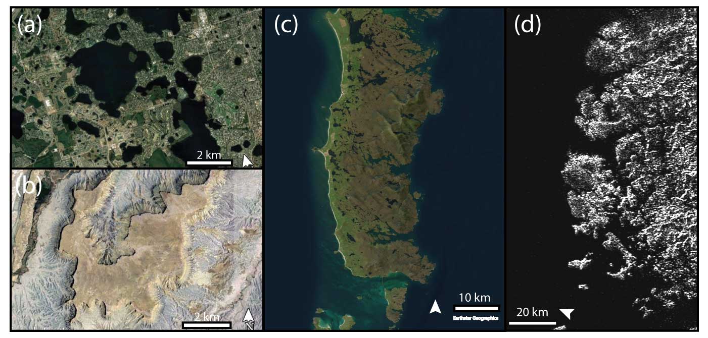
Figure 1 (a) Karst lakes in Florida, USA (© Google Earth, Landsat/Copernicus). Lake Butler and the surrounding region. (b) Caineville Mesa, Utah, USA (© Google Earth, Landsat/Copernicus). (c) South Uist, Scotland (Esri World Imagery, Earthstar Graphics, Esri, 2024). (d) Cassini synthetic aperture radar (SAR) image of Kraken Mare, Titan (NASA).

Although the relative influence of uniform erosion processes such as dissolution and wave-driven erosion is still being quantified (Trenhaile, 2015), the shape of coastlines may offer a means to infer dominant processes in remote environments where in situ measurements are impractical, such as arctic coasts; where local field data are sparse; or on remote planetary bodies, such as Titan (Fig. 1d). A reduced-complexity model of long-term planform evolution of erosion-dominated coasts can provide insights about the importance of wave erosion relative to uniform erosion such as backwasting of permafrost (Günther et al., 2013). Here, we present a reduced-complexity model of detachment-limited coastal erosion in closed basins, such as lakes or inland seas, by uniform erosion and wave erosion. We test the model by comparing our numerical solution of erosion with an analytical solution and test for model result sensitivity to grid resolution and input parameters. Finally, we describe how this model may be applied beyond closed basins to open coasts and islands (see Sect. 5).

2 Background

2.1 Previous models of coastal erosion

2.1.1 Models of wave-driven erosion

Models of rocky-coastline geomorphology have historically focused on the erosion of the cross-shore profile through sea-level rise (Walkden and Hall, 2005; Young et al., 2014), wave impacts (Adams et al., 2002, 2005; Huppert et al., 2020), and the competing effects of sediment abrasion and sediment cover (Kline et al., 2014; Young et al., 2014; Sunamura, 2018; Trenhaile, 2019). But recent work has explored the alongshore variability (Walkden and Hall, 2005) and planform evolution of these features (Limber and Murray, 2011; Limber et al., 2014; Sunamura, 2015; Palermo et al., 2021), with particular focus on either the relationship between planform morphology and retreat rates following storms (Palermo et al., 2021) or the persistence of an equilibrium coastline shape consisting of headlands interspersed with pocket beaches due to variable lithology, grain size, or sediment tools and cover (Trenhaile, 2016; Limber and Murray, 2011; Limber et al., 2014).

Existing models of planform erosion of rocky beaches include (1) a mesoscale (1 to 100 years) alongshore-coupled cross-shore profile model, SCAPE (Walkden and Hall, 2005), in which waves erode the substrate when the substrate is not armored by sediment and sediment is transported by waves using linear wave theory; (2) a numerical model of sea-cliff retreat that focuses on the mechanical abrasion of a notch at the cliff toe and subsequent failure of the cliff and sediment comminution in the surf zone (Kline et al., 2014); and (3) a numerical model of headlands and pocket beaches that takes into account wave energy convergence and divergence and the processes of sediment production and redistribution by waves (Limber et al., 2014).

Previous work on marsh–shoreline erosion considers the heterogeneity of substrate erodibility using a percolation theory model (Leonardi and Fagherazzi, 2015). In this system, low wave energy conditions lead to patchy failure of large marsh portions, resulting in a strong dependence on the spatial distribution of substrate resistance. In contrast, high wave energy conditions cause the shoreline to erode uniformly, such that the spatial heterogeneity in marsh erodibility does not influence the erosion rate (Leonardi and Fagherazzi, 2015). This ignores variations in fetch, which can be important for rocky coastal systems.

These previous process-based models are all computationally expensive and require specific knowledge of sediment and wave characteristics to accurately apply at local scales. To model systems for which minimal field data are available, or to explore the general behavior of planform erosion in rocky coasts under a broad range of conditions, a reduced-complexity model (Ranasinghe, 2020) is necessary.

2.1.2 Models of uniform erosion

Howard (1995) modeled the retreat of a closed-basin scarp as a uniform erosion process. Howard's approach identifies gridded domain points as either interior or exterior to the escarpment and erodes the escarpment edge at a constant rate in all directions originating from adjacent points (Howard, 1995). In these model experiments, the escarpment retreats uniformly toward the interior of the domain from the exterior. This uniform scarp retreat is analogous to coastline retreat in response to the dissolution of a uniform substrate. Although Howard's model was designed for a different, subaerial system, the same process law can describe uniform shoreline erosion along the margins of a liquid-filled closed basin, as we assume the planform shoreline also erodes at the same rate in all directions.

Shorelines formed by dissolution in karst landscapes have received some attention, mostly in the context of cave collapse features or sinkholes (Johnson, 1997; Martinez et al., 1998; Yechieli et al., 2006). However, most research has focused on the initial formation of these features; studies of the long-term retreat of coastlines due to dissolution are focused on the meter-scale erosion of coastal notches through mechanical and biochemical erosion (Trenhaile, 2014, 2015) and to our knowledge have not been evaluated over a larger spatial scale.

3 Model

We developed the Numerical model of coastal Erosion by Waves and Transgressive Scarps V1.0 (NEWTS1.0) (Palermo et al., 2023) to study the planform-shoreline erosion of detachment-limited coasts by waves, uniform erosion, or a combination of these processes. This reduced-complexity model can be used to explore long-term (thousands to millions of years) trends in landscape evolution that result from these processes across the appropriate sea- or lake-level change conditions. Uniform erosion includes dissolution or mass backwasting and is modeled with a spatially uniform rate of shoreline retreat, which generally smooths the coastline and generates cuspate points where promontories are eroded. Wave erosion occurs in proportion to the wave energy that the coastline is exposed to and to the angle of incidence of the incoming waves, such that the erosion rate depends on the wave energy in the cross-shore direction per unit of length along the coast (Komar, 1997; Ashton et al., 2009; Huppert et al., 2020). Coastlines that have larger exposure (larger fetch) experience higher wave energy and therefore faster wave erosion. We model this energy-dependent erosion by computing the fetch of every incident wave angle that may impact a given point on the shoreline and by weighting this fetch by the cosine of the angle between the incident wave crests and the shoreline. Mathematically, this is equivalent to the dot product of the direction of wave travel and the direction normal to the shoreline.

3.1 General description and model setup

3.1.1 Model domain and structure

Model domain

The domain of the model (Fig. 2) is a grid discretized into N_x cells in the x direction and N_y cells in the y direction, with cell spacings Δx and Δy such that x_i=iΔx and y_j=jΔy. The value of each grid cell, z_i,j, corresponds to the landscape elevation. The boundaries of the grid are periodic. Each cell in the domain is defined as either liquid or land based on its elevation relative to sea or lake level. The model could apply to lake level in closed basins or sea level in semi-closed seas or on open coasts. For simplicity, in this paper we will use “lake” to refer to the liquid bodies. “Lake cell” refers to cells occupied by liquid, and “lake level” refers to the elevation of the liquid level. Cells below lake level are fixed and do not erode. Shoreline cells, defined as land cells directly adjacent to liquid, may be eroded by coastal processes through uniform erosion and wave erosion. Lake level is an input to the system that the user can vary throughout a model run.

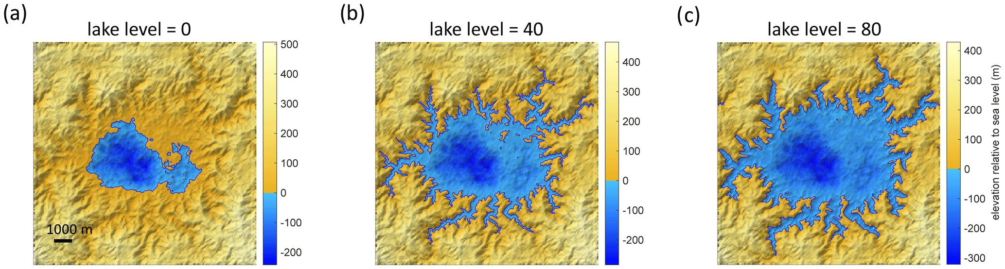
Figure 2 Example model domain with a lake level of (a) 0 m, (b) 40 m, and (c) 80 m. This domain is used in Figs. 4 and 5.

Identification of liquid body and shoreline cells

Boundaries in the grid are identified using pixel connection definitions of either “four-connected”, in which connections occur only across edges, or “eight-connected”, in which connections occur either across edges or at corners. Liquid cells that are eight-connected to each other comprise the same liquid body. The liquid body could represent a sea or lake, so for simplicity we call a liquid cell a lake cell and a liquid body a lake in this paper. Islands are defined as groups of land cells that are surrounded by liquid cells. Lakes can also occur inside islands and islands inside these lakes, so we define a lake hierarchy to identify and model each lake individually. The first level in this hierarchy is the land that is connected to the border of the domain. First-order lakes are lakes that are immediately surrounded by this land that extends to the border of the domain. A first-order island is immediately surrounded by a first-order lake. A second-order lake is surrounded by a first-order island, and so on. This continues such that Nth-order islands are surrounded by Nth-order lakes, and Nth-order lakes are surrounded by N-minus-one-order islands. This hierarchy allows us to identify and isolate unique lakes, which will be important when we consider wave-driven erosion.

Cellular grid erosion

Each cell starts with an initial strength, S_init (see Sect. 3.1.3 to 3.3), which is depleted according to a rate law associated with each coastal process until it reaches 0 (see Sect. 3.2 and 3.3), at which point the cell erodes. Coastal erosion occurs on shoreline cells, defined as land cells adjacent to liquid cells, and decreases the elevation of those cells by a specified depth of erosion, d_e, which is user specified. For cells eroded by coastal processes, $z\left(t\right)=z\left(t-\mathrm{1}\right)-d_{\mathrm{e}}$, where t is model time. For uniform erosion, d_e is conceptualized as the scarp dissolution depth. For wave erosion, it is conceptualized as a wave base. Shoreline cells become lake cells once eroded. To avoid numerical artifacts associated with the time discretization, the time step must be set such that the amount of erosion per iteration is a small fraction of the total cell size. In practice, we set the time step to erode less than $\mathrm{1}/\mathrm{10}$ of a cell at a given time, given the cell spacing and rate law. The model run terminates if a lake cell becomes adjacent to a boundary cell because the wave erosion model requires a closed coastline.

Order of operations

During each time step, erosion occurs according to three steps if enabled: (1) sea- or lake-level change, (2) wave erosion, and (3) uniform erosion (Fig. 3). Here we describe the general model components and simulation procedure. The governing equations for uniform erosion and wave erosion are outlined in more detail in Sect. 3.2 and 3.3, respectively.

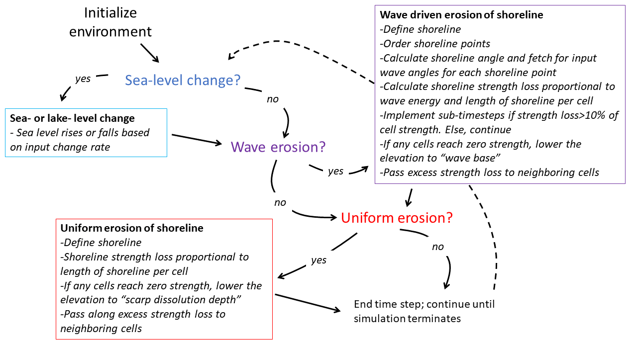
Figure 3 Model structure showing the time loop in which the model (1) updates sea- or lake-level change and then calculates shoreline erosion due to (2) waves and (3) uniform erosion processes.

The first operation of the model is lake-level change. The lake level changes as an input rate or according to an input lake-level curve. The new lake level is used to define the lake(s) and shoreline(s) (Sect. 3.1.1, “Identification of liquid body and shoreline cells”, and 3.1.2).

Next, wave erosion of the shoreline(s) occurs as a function of the fetch – the open-water distance wind and waves travel before reaching a point on the coast – and the angle between the wave crests of the incident waves, φ, and the azimuth of the shoreline, θ (Sect. 3.3). In this module, the shoreline is first identified and traced such that shoreline cells are ordered in a counterclockwise direction. The shoreline is then used to calculate the shoreline angle, incident wave angle, and associated fetch at each cell along the shoreline (Sect. 3.3.1). The elevation of eroded shoreline cells is lowered, their labels are changed to liquid cells as appropriate, and the shoreline is updated (see Sect. 3.4, Fig. 5). This approach considers sediment removal to be instantaneous. Future variations in the model could consider the erosion also to be a function of the height of the material being eroded or of the excavation rate of weathered rubble.

Finally, uniform erosion of the updated shoreline occurs (Sect. 3.2). Here, the shoreline erodes as a function of the alongshore length of the shoreline as measured along cell boundaries (Sect. 3.1.2 and 3.2). And again, the elevation of eroded shoreline cells is lowered, the labels of eroded cells are changed to liquid cells, and the shoreline is updated.

3.1.2 Defining the shoreline

There are two options for defining shoreline cells: the eight-connected case, in which successive land cells along the shoreline may border one another either at cell edges or at cell corners (Fig. 4a), or the four-connected case, in which successive land cells along the shoreline may border one another only at cell edges (Fig. 4b). In the case of an eight-connected shoreline, shoreline cells only border liquid cells at cell edges (Fig. 4a), whereas shoreline cells in a four-connected shoreline can border liquid cells at cell edges or at cell corners (Fig. 4b). We choose Δx and Δy to be small enough to represent the relevant features of the shoreline. If lake-level change occurs in the simulation, the relevant features in the landscape should be taken into account when choosing Δx and Δy. Here we present simulations where Δx and Δy are equal. The model can operate with different Δx and Δy values; however, there could be resulting errors that have not been tested.

Figure 4 Shoreline cells and associated strength loss weighting for a shoreline that is (a) eight-connected or (b) four-connected. Arrows point in the direction of erosion into each shoreline cell from neighboring lake cells. Increasing darkness of shoreline cells indicates increasing strength loss weighting.

The shoreline cells need to be ordered so that the lake can be represented as a polygon for the fetch computation. To order the shoreline cells in closed loops, we start at the first indexed shoreline cell of the longest shoreline and move counterclockwise to find the next shoreline cell. Once a sequence of the first three cells is repeated, the loop is closed and the shoreline is deemed complete. Any remaining shoreline cells that do not lie on this loop represent the shoreline of a separate first-order lake or of an island or higher-order lake contained within the lake. Next, ordering the shorelines of the islands contained within the current lake begins on the first remaining shoreline cell. We repeat this process until all land cells bordering liquid are included in a closed shoreline. When there are multiple first-order lakes in a landscape domain, the shorelines for each lake and its enclosed islands are ordered one at a time.

3.1.3 Cell strength and coastal erosion processes

All cells start with an initial strength, S_init, which represents how difficult it is to erode the land (Eq. 1). We model a material of uniform strength in both planform space and elevation across the domain, but this could easily be extended to a scenario with a material of heterogeneous strength across the domain. The strength of a cell is initialized as a reference strength, S₀, multiplied by the ratio between the cell area, A=ΔxΔy, and a reference cell area, A₀=Δx₀Δy₀, with reference spacing Δx₀ and Δy₀ (Eq. 1). The reference strength and area non-dimensionalize strength and maintain proportions that mitigate discretization bias. The magnitude of these values can be chosen by the user.

$$\begin{array}{}\text{(1)}& S_{\mathrm{init}}=S_{\mathrm{0}}{\displaystyle \frac{A}{A_{\mathrm{0}}}}\end{array}$$

Strength is lost from each shoreline cell at a rate that depends on the exposed perimeter of the cell and an erosion rate law specific to the uniform erosion or wave erosion process. Change in strength is grid-independent for grids sufficiently fine to satisfy model stability because the strength is initialized with a reference cell area in proportion to the parameterized cell area. To mitigate discretization bias, Δx, Δy, and Δt must be sufficiently small so that Δt is less than the time to completely erode a cell (see Sect. 3.2 and 3.3) and that Δx and Δy properly represent the shoreline morphology. In practice, we choose Δx to be equal to Δy.

As time progresses, each shoreline cell loses strength until failure, $S_{i,j}=\mathrm{0}$, at which point the cell has eroded. It is possible for the strength loss in one time step to exceed the remaining strength of the cell. When this occurs, the excess time spent eroding the cell is passed along to all new shoreline neighbors of the eroded cell, representing the time of erosion that neighboring cell will incur after the erosion of the original shoreline. If a new shoreline cell is inheriting excess time from multiple neighbors, the mean excess time is used to compute the strength loss. In our simulations, taking the mean of the excess time resulted in the least grid bias.

Modeled erosion could be underestimated or redistributed improperly if the strength loss for an eroding cell is consistently large relative to the initial strength of the domain. The shoreline would then not update with the newly exposed cells, instead constantly passing strength loss to its neighbors and inaccurately characterizing the morphology. We implement a sub-time-step routine to capture the effect of the changing shoreline within a single time step when the strength loss of any shoreline cell in the domain exceeds a certain threshold of the initial strength, α, which ranges between 0 and 1. In the modified time-step routine, the damage is computed and the shoreline updated in sub-time steps, which segments the time step and allows erosion to occur in smaller increments.

3.2 Uniform erosion model

The rate of shoreline retreat by uniform erosion is set by an erodibility coefficient, k_uniform (Eq. 2). Strength loss due to uniform erosion occurs as a function of the amount of shoreline in contact with the lake for a given cell, represented as the number of four-connected sides and eight-connected corners, c, in contact with lake cells (Eq. 3; Fig. 4). Because the diagonal of the cell is longer than the side by a factor of $\sqrt{\mathrm{2}}$, it would take $\sqrt{\mathrm{2}}$ times longer for a shoreline to retreat across a cell diagonally than in the perpendicular direction. To correct for this in our model, the strength loss computed from an exposed corner is $\sqrt{\mathrm{2}}/\mathrm{2}$ times as much as the strength lost from an exposed side.

$$\begin{array}{}\text{(2)}& {\displaystyle \frac{\mathrm{d}x}{\mathrm{d}t}}=k_{\mathrm{uniform}}\text{(3)}& {\displaystyle \frac{\mathrm{\Delta }{S}_{i,j}}{S_{\mathrm{0}}}}=-k_{\mathrm{uniform}}\left(s_c+{\displaystyle \frac{\sqrt{\mathrm{2}}c}{\mathrm{2}}}\right){\displaystyle \frac{\mathrm{\Delta }x}{\mathrm{\Delta }{x}_{\mathrm{0}}}}\mathrm{\Delta }t\end{array}$$

3.3 Wave erosion model

Wave erosion occurs at a rate determined by a wave erodibility coefficient, k_wave (m yr⁻¹), and the wave energy in the cross-shore direction, E (Eq. 4). The wave energy depends on the wave height, H; the angle between the wave crests of the incident waves, φ; and the azimuth of the shoreline, θ (Eq. 5). Wave height scales with fetch, F, such that $H\propto \sqrt{F}$ (Hasselmann et al., 1973; Lamont-Smith and Waseda, 2008). Therefore, we use fetch to approximate the wave energy density for a wave from a given direction on a coastline (Eq. 6). The use of wave energy implies the assumption of single-period waves.

$$\begin{array}{}\text{(4)}& {\displaystyle \frac{\mathrm{d}x}{\mathrm{d}t}}=k_{\mathrm{wave}}E\text{(5)}& {\displaystyle }E={\displaystyle \frac{\mathrm{1}}{\mathrm{16}}}\mathit{\rho }g{H}^{\mathrm{2}}\cos (\mathit{\phi }-\mathit{\theta })\text{(6)}& {\displaystyle }E\propto \mathit{\rho }gF\cos (\mathit{\phi }-\mathit{\theta })\end{array}$$

The strength loss of a cell due to waves can be described as

$$\begin{array}{}\text{(7)}& {\displaystyle \frac{\mathrm{\Delta }{S}_{i,j}}{S_{\mathrm{0}}}}=-k_{\mathrm{wave}}(s_c+{\displaystyle \frac{\sqrt{\mathrm{2}}c}{\mathrm{2}}})\underset{\mathit{\phi }=\mathrm{0}}{\overset{\mathrm{2}\mathit{\pi }}{\int }}F\left(\mathit{\phi }\right)\cos (\mathit{\phi }-\mathit{\theta })\mathrm{d}\mathit{\phi }{\displaystyle \frac{\mathrm{\Delta }x}{\mathrm{\Delta }{x}_{\mathrm{0}}}}\mathrm{\Delta }t.\end{array}$$

If the strength loss in a time step exceeds a parameter-set threshold, a sub-time-step routine is implemented. Because the fetch calculation is the costliest step of the model, in this sub-time-step routine, we estimate the fetch weighting by interpolating the fetch of the nearest-neighbor shoreline cells. This avoids additional costly fetch computations during the sub-time-step updates and allows us to approximate erosion driven by waves in a way that limits error without slowing down the model simulation.

3.3.1 Modeling wave energy density

The rate of strength loss of each shoreline cell is proportional to the wave energy density. We model the wave energy density to be proportional to the fetch and the cosine of the angle between the incident wave crest and the shoreline (Fig. 5). To compute this quantity, we measure the fetch in all directions around the shoreline, in increments of dφ, for each shoreline cell. For each direction, we extend a ray from the cell center in the direction 90° − φ and step along the ray in increments of a distance δ until reaching the opposite shore. The modeling approach presented here does not consider the effects of shoaling or refraction, so waves that would approach the shoreline from beyond 90° are not considered. When the ray extends past the opposite shoreline, we take one step back and define this point as the intersection. The distance between this intersection and the originating shoreline cell center is the fetch in the direction from which a wave would propagate (Fig. 4b). The length of fetch may be truncated at an input maximum length, which would represent the distance at which waves saturate and do not continue to grow. To calculate the amount of strength loss each cell incurs, we compute the area of a polygon defined by the ray–shoreline intersections for that cell (Fig. 5a). We call this area the “fetch area”. The length of the ray in each direction is then weighted by the cosine of the angle between the shoreline and the incident wave crest, φ−θ (Fig. 5a). The area of the polygon defined by these cosine-weighted fetch lengths is computed and called the “wave area”. The wave area for each point on the shoreline approximates the integral in Eq. (7).

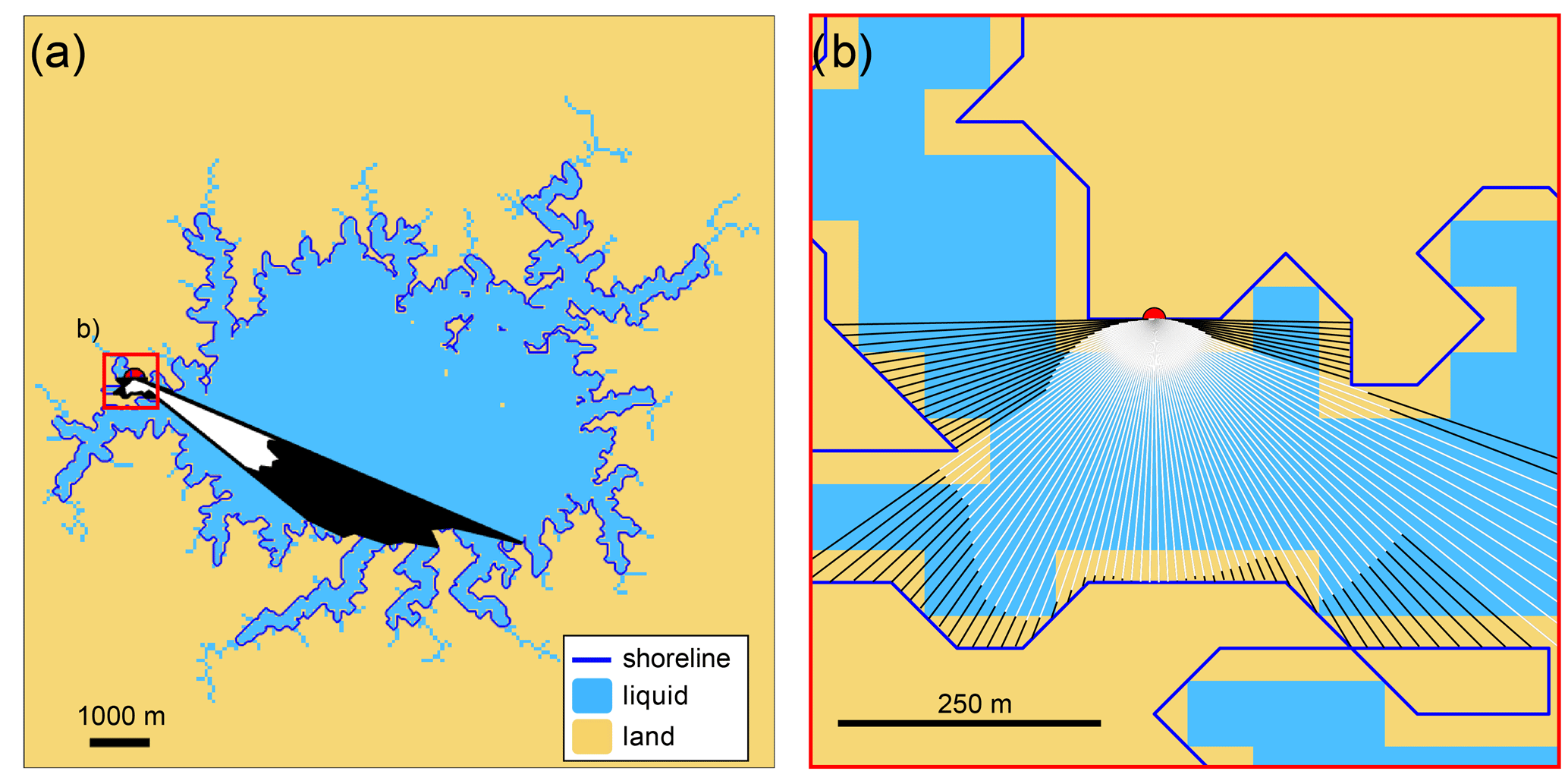
Figure 5 (a) Fetch area (black) and wave area (white) computed for a point (red circle) on a typical model shoreline (blue). The area shown in (b) is outlined in red. (b) Zoomed-in view of fetch line-of-sight rays (black) and angle-weighted line-of-sight rays (white) computed for the same point. In this example, dφ=2°, and the ray step size is δ=0.05 m.

3.4 Model output

The model can be initialized with any user-defined topographic model. In the simulations presented here, we initialize the grid with a synthetic topography consisting of a pseudo-fractal surface with variance of 10 000 superimposed on an elliptical depression with a depth of 25 % of the domain relief and eroded by river incision to 95 % of the initial terrain relief using a landscape evolution model (Perron et al., 2008, 2009, 2012). We then flood the domain by raising the lake level by 40 m. The model of shoreline retreat by uniform and wave erosion is then applied to the domain. Here, we show examples of an initial landscape eroded by either wave erosion or uniform erosion to illustrate separately the effects of the two erosional mechanisms in the model (Fig. 6). However, all model components may be run in combination. We do not provide examples of combined uniform and wave erosion models here.

The initial shoreline exhibits a dendritic shape due to flooding of the incised river valleys (Fig. 6). Through time, the uniform erosion model drives shoreline retreat at the same rate everywhere around the perimeter of the lake, resulting in widening valleys and increasing the pointedness of promontories or headlands (Fig. 6). The overall shape of the lake is maintained but becomes smoother and tends toward circular. In the case of wave erosion, the river valleys erode slowly while the exposed parts of the coast erode more rapidly (Fig. 6). The embayed river valleys largely maintain their shapes, whereas the central, high-fetch portion of the coast grows larger and smoother.

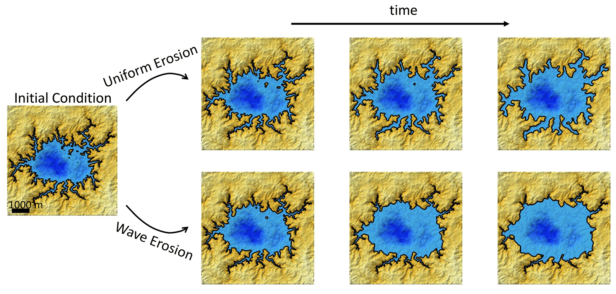
Figure 6 Shaded relief maps of example model simulations of uniform erosion and wave erosion through time, starting from the same initial condition. Blue color indicates liquid cells, with darker blues indicating deeper depths. Gold color indicates land cells, with lighter shades indicating higher elevations. Black lines trace shorelines. Erodibility coefficients are $k_{\mathrm{wave}}=k_{\mathrm{uniform}}=\mathrm{0.00001}$ m yr⁻¹. Uniform erosion (top) results in greater overall smoothness that is punctuated by pointy headlands, whereas wave erosion (bottom) results in blunted headlands, smooth open sections of coast, and preservation of sharp features in sheltered areas. Landscape time steps shown correspond to similar amounts of erosion between wave and uniform examples. The shoreline is defined as four-connected in these examples.

To test our model performance, we compare the planform morphologies of model output with example shorelines that have known geomorphic processes. While long-term coastal cliff retreat rates could be determined using dating techniques at local field sites (Hurst et al., 2016; Bossis et al., 2024), more detailed testing of the model would require re-creation of the plan-view shape at a broader scale. Because long-term changes in planform morphology during retreat of bedrock coastlines are generally too slow to be measurable with historical aerial and satellite images, the data needed to fully validate this model are not presently available. Nonetheless, a visual comparison can be drawn between coastal features found on Earth and the coastline shapes generated by each end-member erosional mechanism in the model, which is the main goal of our modeling approach. These shorelines exhibit the same overall smoothness punctuated by sharp headlands as is seen in the shorelines formed by uniform erosion in our model (Fig. 6). Although it is beyond the scope of this paper, output from this model could be used to quantitatively describe shoreline morphologic differences driven by wave and uniform erosional processes or signatures of sea- or lake-level changes.

A bedrock lake that has been eroded recently by waves is exemplified by Lake Rotoehu, New Zealand (Fig. 7c). In this example, we observe blunted headlands and smooth, rounded stretches in open sections of coast and crenulated shorelines in more protected areas of coast – similar to the shorelines formed by wave erosion in our model (Fig. 6).

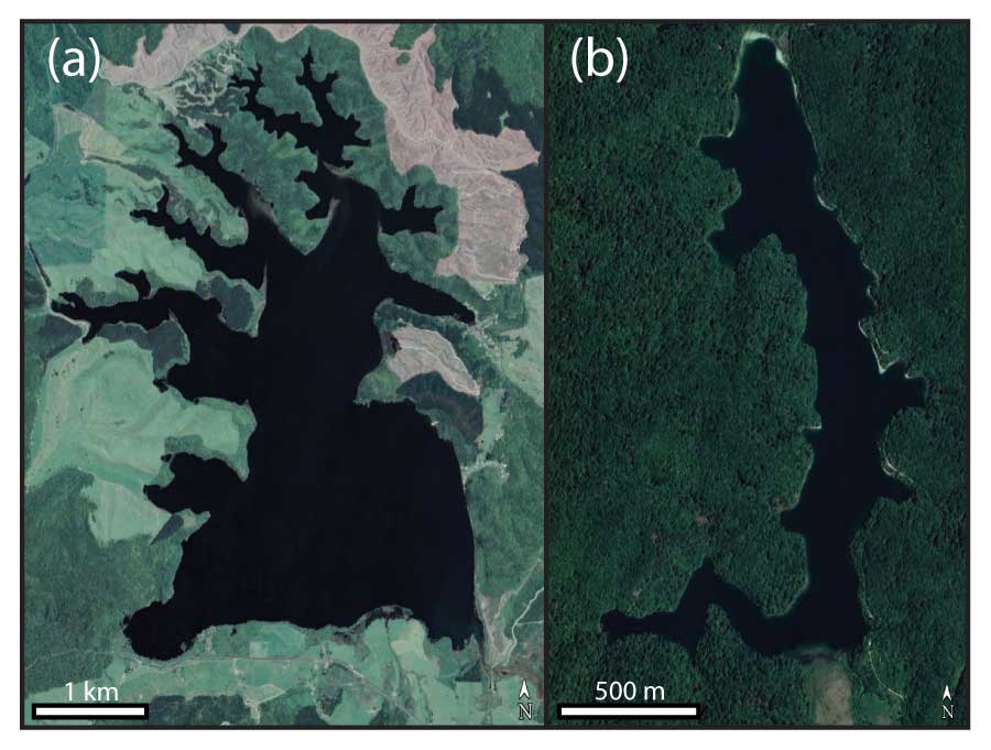
Figure 7 (a) Lake Rotoehu, New Zealand (© Google Earth, CNES/Airbus). (b) Plitvice Lake, Croatia (© Google Earth, DigitalGlobe).

4 Model tests

4.1 Comparison with analytical solution and sensitivity to shoreline connectedness

For the simple case of an initially circular shoreline, we compute the shoreline evolution analytically and compare this known solution with our numerical model results. For the uniform erosion case, the rate at which the radius of a circle increases, $\dot{r}$, is equal to the constant of erosion, in this case k_uniform.

$$\begin{array}{}\text{(8)}& \dot{r}\left(t\right)=k_{\mathrm{uniform}}\end{array}$$

Therefore, the radius, r, at time, t, and initial radius, r₀, for uniform erosion is

$$\begin{array}{}\text{(9)}& r\left(t\right)=r_{\mathrm{0}}+k_{\mathrm{uniform}}t.\end{array}$$

For wave erosion, the rate of increase in the radius, $\dot{r}$, depends on the constant of erosion, k_wave, and the integral of the fetch, F, at each angle between the incoming wave crest and the shoreline (φ−θ) in all directions around the circle:

$$\begin{array}{}\text{(10)}& {\displaystyle }F\left(\mathit{\phi }\right)=r\sqrt{\mathrm{2}(\mathrm{1}+\cos (\mathrm{2}\left(\mathit{\phi }-\mathit{\theta }\right)\left)\right)},\text{(11)}& {\displaystyle }\dot{r}\left(t\right)={\displaystyle \frac{k_{\mathrm{wave}}}{\mathrm{2}}}\underset{-\frac{\mathit{\pi }}{\mathrm{2}}}{\overset{\frac{\mathit{\pi }}{\mathrm{2}}}{\int }}(F\left(\mathit{\phi }\right)\cos \left(\mathit{\phi }-\mathit{\theta }\right){)}^{\mathrm{2}}\mathrm{d}\mathit{\phi }.\end{array}$$

Computing this integral simplifies to

$$\begin{array}{}\text{(12)}& \dot{r\left(t\right)}=k_{\mathrm{wave}}{\displaystyle \frac{\mathrm{3}\mathit{\pi }}{\mathrm{4}}}r(t{)}^{\mathrm{2}}.\end{array}$$

Therefore, the radius, r, at time, t, for wave erosion is

$$\begin{array}{}\text{(13)}& r\left(t\right)={\displaystyle \frac{r_{\mathrm{0}}}{\mathrm{1}-r_{\mathrm{0}}{k}_{\mathrm{wave}}\frac{\mathrm{3}\mathit{\pi }}{\mathrm{4}}t}}.\end{array}$$

We use the analytical solution for the radius through time for each case to calculate the shoreline position and area of the circular lake as it is eroded by either uniform erosion or wave erosion. To compute the relative error in the numerical model, a test circular lake is eroded for 17 400 years, resulting in an approximately 20 % and 25 % increase in lake area for wave and uniform erosion, respectively, and compare this to the analytical solution.

Because the model operates on a rectangular grid, some amount of distortion of a circle is expected. While this distortion cannot be avoided entirely by increasing the grid resolution, increasing it can reduce the error in the shoreline shape by allowing the shoreline to retreat in finer increments. A fine grid, however, comes at increased computational cost. The spatial resolution, Δx and Δy, should be chosen to be small enough to represent the features of the shoreline but large enough to keep computational costs reasonable.

We perform these simulations for uniform and wave erosion with both the four-connected version and the eight-connected version of the model (Fig. 4). The four-connected model performs significantly better than the eight-connected model, as shown by the relative error in lake area. The four-connected case maintains a relative error of less than 2 % throughout the simulation, whereas the error in the eight-connected model increases roughly linearly with time, ending at approximately 7 % (Fig. 8a). The distortion is worse in the eight-connected case for both uniform erosion and wave erosion and systematically worse in the diagonal directions (Fig. 8b, c). This analysis suggests that grid bias is a more important source of error in the model than spatial discretization.

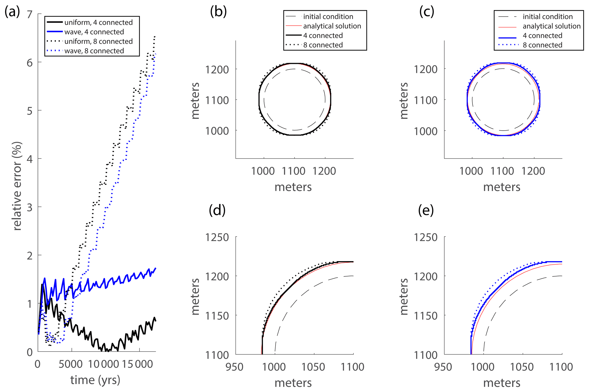
Figure 8 (a) The error in lake area through time of an initially circular lake relative to the analytical solution for four-connected (solid) and eight-connected (dotted) models of uniform erosion (black) and wave erosion (blue). The initial condition (dashed), analytical solution (red), and modeled four-connected and eight-connected shorelines at time = 17 400 are shown for (b) uniform erosion and (c) wave erosion, with zoomed-in results shown for (d) uniform erosion and (e) wave erosion.

4.2 Resolution sensitivity

4.2.1 Grid resolution

Although the grid resolution affects the size of the features that can be resolved in the landscape, it does not substantially affect the amount of coastal erosion. As discussed above, the strength loss in this model is insensitive to grid resolution, Δx, and time step, Δt, assuming that Δx is fine enough to resolve the features of interest and that Δt is small enough to limit erosion to less than the maximum cell strength in a single time step. The total amount of strength in the domain is independent of Δx because the number of cells is proportional to Δx⁻², and the strength of each cell is proportional to Δx². The damage in each time step is independent of Δx because the number of cells on the shoreline is proportional to Δx⁻¹, and the damage per cell is proportional to Δx.

4.2.2 Threshold strength parameter

The threshold strength parameter, α, was introduced to prevent excess strength reduction from being neglected when a cell has less strength than is depleted in a time step. A smaller threshold strength parameter results in a more frequent application of the sub-time-step routine and in smaller sub-time steps. With a less stringent threshold strength parameter (>0.05), the shoreline may erode more than the analytical solution in a time step, leading to a positive slope in the relative error in strength against the threshold strength parameter (Fig. 9).

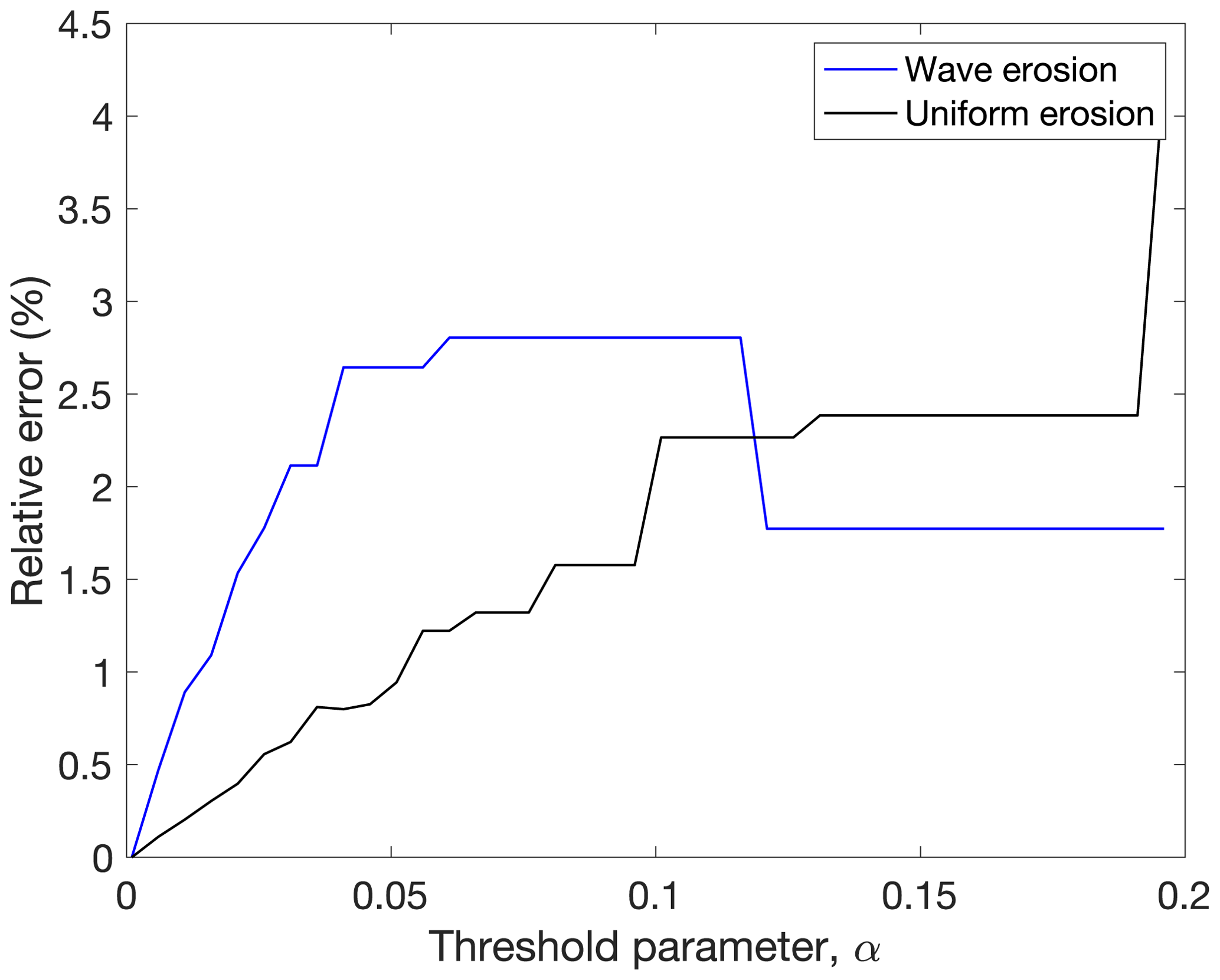
Figure 9 Error in total strength reduction as a function of the threshold strength parameter, expressed as a percentage of the error for the smallest value of the threshold strength parameter, for the initial condition in Fig. 6 eroded over one time step by uniform erosion (black) and wave erosion (blue).

4.3 Fetch ray angular and distance increments

We test the sensitivity of the fetch area calculation to the angle between rays, dφ, and the ray step size, δ. This test allows us to analyze the error in fetch of a typical model due to these parameters. The error measurements provide a basis for selecting an angle between rays and a ray step size that optimizes the trade-off between computational time and model accuracy.

We compute the error in fetch area over a range of ray angles and step sizes. With a fixed ray step size of 0.05Δx (the nominal step size used in our simulations), we compute the fetch error for each shoreline cell over a range of 0.012 to 10°, corresponding to 30 000 and 36 rays, respectively. With a fixed ray angle of 2° (the nominal ray angle used in our simulations), we compute the relative fetch error over a range of ray step sizes between 0.01Δx and Δx. The fetch area error in each cell is computed relative to the fetch area of the finest resolution in each parameter: 2° between rays and a ray step size of 0.05Δx (Fig. 10). The error, as well as the standard deviation in errors, in each scenario converges to zero, indicating that as the angle between rays and the ray step size become small, the fetch area converges to a constant value.

Figure 10 Relative error in fetch area for a range of step sizes with a ray angle of 2° (black) and for a range of ray angles with a step size of 0.05Δx (red).

5 Discussion and conclusions

In this paper, we present NEWTS1.0, a cellular model of coastline erosion in detachment-limited environments by uniform erosion and by wave erosion. For uniform erosion, the coastline erodes at a constant rate everywhere along the shoreline. For wave-driven erosion, the coastline erodes as a function of the fetch and the angle between the incident waves and the shoreline.

While our uniform erosion rate law is similar to that of Howard (1995), our modeling approach is different. Because there are multiple mechanisms that may erode a coast in our model, memory of the strength loss of the substrate is necessary. Rather than rays extending at a constant rate from the interior points representing retreat as is done in Howard's (1995) model, the strength of shoreline (or scarp edge) points is reduced by an amount proportional to the number and direction of neighboring lake cells.

Our wave erosion model contains a dependence on wave energy like in other models (Walkden and Hall, 2005; Limber et al., 2014) but simplifies the influence of sediment and other factors to a constant. This simplification is useful for locations without readily available grain size or sediment cover data and to investigate the long-term influence of these processes. However, a limitation of this simplified approach is the implicit assumption of a single wave period when using wave energy rather than wave power in the wave erosion rate law (Eqs. 4–6). Future work could extend the capabilities to include consideration of wave period.

Our model is also unusual among coastal erosion models in that it evaluates multiple closed coastlines (or lakes) in a landscape domain rather than a single reach of open coastline and in that it focuses on the planform morphology of eroding rocky closed-basin shorelines. A limitation of this model is that sediment redistribution is not included in the erosion rate laws, and there is no sedimentation along the coast. Sediment abrasion and cover could be incorporated in future versions of our model through a spatially heterogeneous and time-dependent erodibility coefficient, k; however, this would likely require parameterization from field data.

While this model is currently configured to simulate the erosion of closed basins such as lakes or inland seas, modifications could be made to evaluate open stretches of coast. The two model algorithms that would need to be considered are the routines to order the shoreline and to compute fetch. The routine to order the shoreline requires the shoreline to be a closed loop. To evaluate an open stretch of coast in the model, the landscape domain could be modified to artificially enclose either the open coast or the boundary conditions. The simpler approach is to modify the landscape domain such that an artificial and large basin is made surrounding the domain, defining the artificial basin boundary cells as fixed points that do not erode and making sure that the modified landscape is further than the fetch saturation length from the shoreline of interest. To evaluate an ocean island, enclose it in land beyond the fetch saturation length in distance from the island. If the domain is modified such that the shoreline is a closed loop, all routines should function appropriately. However, if a different routine to order the shoreline is used, the fetch computation would need to be slightly modified. Currently, fetch is computed as an extended ray from a shoreline cell that advances at some interval length until it reaches land and allows for a fetch threshold at some length of wave saturation (see Sect. 3.3.1). The truncation of computed fetch at the threshold length is implemented following the calculation of the fetch length. If there is no land on the opposite side of the ray, an error would occur. Therefore, by truncating the fetch length as the ray is extending rather than after the opposite land is found, fetch could be calculated for open coasts. A more complicated but preferable approach would be to change the boundary conditions. If the boundaries of the open stretch of coast were periodic in the alongshore direction, the entire coast could retreat without introducing an artificial boundary edge and a larger domain. If a fetch vector went off the periodic boundary, it would wrap around to the other side and continue. If a periodic boundary condition is deemed inappropriate for a specific model task, mirrored boundaries in the alongshore direction could be used instead. The shape of the coast would be reflected in each boundary, and fetch vectors would reflect off the boundary.

As a reduced-complexity model, NEWTS1.0 can be applied to investigate coastal systems in remote environments where fieldwork is difficult or impossible. This includes locations such as the Arctic or Saturn's moon Titan, home to the only other active coastlines in our solar system. The simplicity of our model allows for efficient long-term simulations of coupled landscape evolution and coastal erosion in detachment-limited systems. Among coastal systems on Earth, investigations of fetch dependence and the resulting morphology given a combination of erosional mechanisms would be particularly relevant to the carbonate geomorphology community, as dissolution and wave activity are both often acting simultaneously along these coasts.