Focal-TSMP: deep learning for vegetation health prediction and agricultural drought assessment from a regional climate simulation

Satellite-derived agricultural drought indices can provide a complementary perspective of terrestrial vegetation trends. In addition, their integration for drought assessments under future climates is beneficial for providing more comprehensive assessments. However, satellite-derived drought indices are only available for the Earth observation era. In this study, we aim to improve the agricultural drought assessments under future climate change by applying deep learning (DL) to predict satellite-derived vegetation indices from a regional climate simulation. The simulation is produced by the Terrestrial Systems Modeling Platform (TSMP) and performed in a free evolution mode over Europe. TSMP simulations incorporate variables from underground to the top of the atmosphere (ground-to-atmosphere; G2A) and are widely used for research studies related to water cycle and climate change. We leverage these simulations for long-term forecasting and DL to map the forecast variables into normalized difference vegetation index (NDVI) and brightness temperature (BT) images that are not part of the simulation model. These predicted images are then used to derive different vegetation and agricultural drought indices, namely NDVI anomaly, BT anomaly, vegetation condition index (VCI), thermal condition index (TCI), and vegetation health index (VHI). The developed DL model could be integrated with data assimilation and used for downstream tasks, i.e., for estimating the NDVI and BT for periods where no satellite data are available and for modeling the impact of extreme events on vegetation responses with different climate change scenarios. Moreover, our study could be used as a complementary evaluation framework for TSMP-based climate change simulations. To ensure reliability and to assess the model’s applicability to different seasons and regions, we provide an analysis of model biases and uncertainties across different regions over the pan-European domain. We further provide an analysis about the contribution of the input variables from the TSMP model components to ensure a better understanding of the model prediction. A comprehensive evaluation of the long-term TSMP simulation using reference remote sensing data showed sufficiently good agreements between the model predictions and observations. While model performance varies on the test set between different climate regions, it achieves a mean absolute error (MAE) of 0.027 and 1.90 K with coefficient of determination (R²) scores of 0.88 and 0.92 for the NDVI and BT, respectively, at 0.11° resolution for sub-seasonal predictions. In summary, we demonstrate the feasibility of using DL on a TSMP simulation to synthesize NDVI and BT satellite images, which can be used for agricultural drought forecasting. Our implementation is publicly available at the project page (https://hakamshams.github.io/Focal-TSMP, last access: 4 April 2024).

1 Introduction

According to recent studies on historical trends and current projections, different regions of the Earth would be under a changing climate more vulnerable to extreme events such as flash droughts (Christian et al., 2021, 2023; Yuan et al., 2023), meteorological and agricultural droughts (Essa et al., 2023), forest wildfires (Patacca et al., 2023), and water storage deficiency (Pokhrel et al., 2021). The expected increase in concurrence of agricultural droughts would cause crop production losses and vegetation mortality. In particular, people in regions with fragile adaptation and mitigation strategies would be more affected. Therefore, forecasting the vegetation responses and their evolving patterns conditioned on climate scenarios is a requirement to form better mitigation and adaptation strategies.

In relation to this, there has been a growing line of research in the past on improving and deploying climate modeling that attempts to simulate the underlying processes of the Earth system (Shrestha et al., 2014; Gasper et al., 2014; Lawrence et al., 2019). These modeling platforms are essential for realizing and forecasting climatic extreme events such as droughts in a model simulation (Miralles et al., 2019). For instance, the simulated outputs of modeling systems can be used to derive agricultural drought indices based on a deficiency in precipitation (McKee, 1995; Vicente-Serrano et al., 2010) or soil moisture (Martínez-Fernández et al., 2015). Nowadays, satellite observations around the world provide a near-real-time global monitoring of vegetation and drought conditions. Vegetation products derived from satellite land surface reflectances can be used as proxies for vegetation health and consequently as agricultural drought indicators (Qin et al., 2021; Vreugdenhil et al., 2022). While historical trends in satellite-based droughts have been extensively studied, satellite-based agricultural drought assessment and its relation to climate simulations under climate change remains not fully explored. In this study, we propose to use deep learning (DL) to improve the agricultural drought analysis by predicting satellite-derived vegetation indices that can be combined with meteorological or hydrological indices which are often used in studies of drought assessment to provide more comprehensive assessments. In fact, some studies highlighted inconsistencies in the long-term drought trends (Sheffield et al., 2012; Kew et al., 2021; Vicente-Serrano et al., 2022). Meanwhile, others showed a different perspective of trends related to terrestrial vegetation from remote sensing products (Zhu et al., 2016; Kogan et al., 2020). This is usually explained as assessments are highly dependent on drought definition (Satoh et al., 2021; Reyniers et al., 2023) and extreme event attribution (Van Oldenborgh et al., 2021), i.e., the drought indicator that was chosen in the methodology and the variations in modeling platforms. In addition, prescribed vegetation assumptions exist in climate simulations which limit the modeling of atmospheric carbon effects or soil moisture deficiency on vegetation (Pirret et al., 2020; Pokhrel et al., 2021; Reyniers et al., 2023). If we add to this the complex spatiotemporal response of vegetation to climate variability (Seneviratne et al., 2021; Jin et al., 2023), i.e., regional responses to climate have different dynamics and are more complicated than those on a global scale, we can conclude that predicting the vegetation state in response to drought under climate conditions still poses a major challenge. More precisely, in this study we predict satellite-based vegetation products from a free, evolving simulation based on the Terrestrial Systems Modeling Platform (TSMP) (Furusho-Percot et al., 2019a). TSMP simulations integrate variables from groundwater to the top of the atmosphere (ground-to-atmosphere; G2A) and are primarily employed in studies on the water cycle and climate change (Ma et al., 2021; Furusho-Percot et al., 2022; Naz et al., 2023; Patakchi Yousefi and Kollet, 2023). In particular, we predict from the TSMP simulation the normalized difference vegetation index (NDVI) and brightness temperature (BT) as they would have been observed from the Advanced Very-High-Resolution Radiometer (AVHRR) from the National Oceanic and Atmospheric Administration (NOAA) satellite systems. The NDVI is computed from the reflectance in visible red (ρ_R) and near-infrared (ρ_NIR) bands. It is a standard product that is extensively used in applications for vegetation health and crop yield (Tucker, 1979). BT is a calibrated spectral radiation derived from the thermal band (ρ_IR) and can be used for temperature-related vegetation stress monitoring (Kogan, 1995a). We assume that a climate simulation (i.e., TSMP simulation) that is close to the true state of the Earth should be able to model vegetation products (i.e., NDVI and BT) regardless of the target satellite platform (in this study, the AVHRR from the NOAA). Recently, DL models have become popular for building a predictive model for tasks that include complex or intractable cause-and-effect relations within the Earth system (Bergen et al., 2019; Tuia et al., 2023; de Burgh-Day and Leeuwenburg, 2023). In addition, DL can be used to handle biases implicitly, thus simplifying the entire workflow (Schultz et al., 2021). For instance, DL was recently used in climate modeling for bias correction and downscaling to project extremes (Blanchard et al., 2022), weather forecasting (Lam et al., 2022; Chen et al., 2023; Bi et al., 2023; Ben-Bouallegue et al., 2023), supporting data assimilation systems (Düben et al., 2021; Valmassoi et al., 2022; Yu et al., 2023), and generalized multi-task learning (Nguyen et al., 2023; Lessig et al., 2023). In this work, we thus propose a DL approach based on focal modulation networks (Yang et al., 2022) to simultaneously predict the NDVI and BT from the model simulation. In this way, we leverage a climate simulation for long-term forecasting and DL for mapping the forecast variables to vegetation-related indices that are not part of the simulation model.

Forward operators like radiative transfer solvers are normally used to synthesize spectral band satellite images from the output of a numerical weather model (Scheck et al., 2016; Geiss et al., 2021; Li et al., 2022). In this paper, we investigate the use of DL to predict products of atmospherically corrected albedo and emissivity on land (atmospherically corrected bottom of atmosphere) like the NDVI and BT simultaneously rather than training the neural network to serve as an emulator for a predefined physical-based radiative transfer model. In other words, our training data for DL are derived from real-world satellite observations (empirical operator) without assimilating data or assumptions about radiations. Besides, there are climate–vegetation models which directly simulate the vegetation dynamic based on ecological processes and statistical modeling. Nevertheless, they are limited by the complexity of the processes and poor generalization (Chen et al., 2021). Unlike hydro-meteorological variables that can be predicted or forecast using a numerical weather model, vegetation products demand an extended modeling representation of the surface and sub-surface (Lees et al., 2022). Recently, Salakpi et al. (2022a, b) predicted short-term vegetation products based on previous vegetation conditions and observational anomaly indices in a Bayesian auto-regressive approach. However, the interaction between vegetation and climate variability exhibits a strong non-linear behavior. In this respect, many studies explored the applicability of DL for vegetation health prediction using climate models and remote sensing data (Das and Ghosh, 2016; Adede et al., 2019; Ferchichi et al., 2022; Wu et al., 2020; Kraft et al., 2019; Prodhan et al., 2021). A common approach is to use past vegetation conditions to predict the short-term future variations (Nay et al., 2018; Yu et al., 2022; Hammad and Falchetta, 2022; Lees et al., 2022; Vo et al., 2023). In a related work, Requena-Mesa et al. (2021) addressed the problem of optical satellite imagery forecasting as a guided video prediction task. In their framework, vegetation dynamics approximated by the NDVI are modeled at high resolution using past satellite images as initial conditions and static and reanalysis data as a model guidance. Similar approaches with this framework were presented in Robin et al. (2022), Kladny et al. (2022), and Diaconu et al. (2022) and on a continental scale in Benson et al. (2023). While these works differ in their methodologies, i.e., in the predicted vegetation products, model architectures, and spatiotemporal resolutions, they have a good performance overall for short-term forecasting. Although short-term forecasting, i.e., for a few weeks, is very useful for short-term planning, a more significant contribution could be achieved with a much longer forecasting time (Marj and Meijerink, 2011). Nonetheless, only few studies addressed the forecasting of long-term vegetation conditions (Marj and Meijerink, 2011; Miao et al., 2015; Patil et al., 2017; Chen et al., 2021; Wei et al., 2023). In addition, most studies focused only on a single indicator. The combination of different indicators like the NDVI and BT with their corresponding drought indices provides complementary information on the vegetation state and is beneficial for vegetation monitoring (Yang et al., 2020). As mentioned before, we aim to use DL to predict vegetation products like the NDVI and BT from a regional climate simulation on a continental scale. We also focus on long-term forecasting without using an initial state, i.e., satellite images from previous time steps. Unlike aforementioned works, we use more input data for the neural network from the surface and sub-surface to account for a more detailed representation of the reflectance and emissivity on the ground. In addition, we built the neural network on vision transformers (Dosovitskiy et al., 2021) and convolutional neural network (CNN) models taking into account the spatial context around each input pixel and operating on the whole scene at once. This was motivated by previous studies that indicate that an effective model of the environment should consider the spatial correlation within the domain. Previous works train and evaluate DL models on bias-corrected reanalysis data. In contrast, we evaluate the approach with real-world observations using a run of the simulation in the past. It is worth noting that this evaluation is more consistent with real-world deployment schemes, since it is questionable how a model that has been trained and evaluated on reanalysis data will perform on biased climate projection simulations. Thus, we opt for a simulation that mimics a climate projection of the past and train and evaluate the model on it to internally correct biases and predict vegetation products.

To showcase the potential of our approach, we apply the predicted NDVI and BT for long-term agricultural drought forecasting, where we derive the vegetation condition index (VCI), thermal condition index (TCI), and vegetation health index (VHI) (Yang et al., 2020) as agricultural drought indicators from the predicted NDVI and BT. As part of this, we analyze whether a DL model trained on a simulation produced by the TSMP can be used for vegetation health forecasting on a continental scale by identifying regions and periods of uncertainty in the model prediction. Moreover, we analyze the importance of the input explanatory variables. We achieve an overall mean absolute error (MAE) of 0.027 and 1.90 K with coefficient of determination (R²) scores of 0.88 and 0.92 in predicting the NDVI and BT, respectively, for sub-seasonal predictions at 0.11° resolution. Our results indicate that a direct prediction of vegetation products from a TSMP simulation with DL is an effective way for scenario-based assessments of vegetation response to climate change.

The rest of this article is organized as follows. Section 2 describes the datasets that are used in the experiments. The methodology is described in Sect. 3. Experimental results and an analysis on variable importance are given in Sect. 4. Finally, conclusions are provided in Sect. 5.

2 Datasets and data preprocessing

In this section, we describe the datasets used in the experiments. The TSMP simulation is presented in Sect. 2.1, the observational remote sensing data for model training and evaluation are presented in Sect. 2.2, and the preprocessing framework of the data is described in Sect. 2.3.

2.1 Regional Earth system simulation

For this study, we use the simulation produced by the Terrestrial System Modeling Platform (TSMP) version 1.1. at the Institute of Bio- and Geosciences – Agrosphere (IBG-3) of the Jülich Research Centre (FZJ) and originally described in Shrestha et al. (2014) and Gasper et al. (2014). The simulation used in this study is introduced in Furusho-Percot et al. (2019a). The TSMP is a physics-based integrated simulation representing a realization of the terrestrial hydrologic and energy cycles that cannot be directly obtained from measurements. Its setup consists of three main interconnected model components:

• The Consortium for Small-scale Modeling (COSMO) version 5.01 is a numerical weather model to simulate the diabatic and adiabatic atmospheric processes (Baldauf et al., 2011).

• The Community Land Model (CLM) version 3.5 is used to simulate the bio-geophysical processes on the land surface (Oleson et al., 2004, 2008).

• ParFlow version 3.2 is a hydrological model that explicitly simulates the 3D dynamic processes of water in the land surface and underground (Jones and Woodward, 2001; Kollet and Maxwell, 2006; Jefferson and Maxwell, 2015; Maxwell et al., 2015; Kuffour et al., 2020).

ECMWF ERA-Interim data (Dee et al., 2011) were used to define the initial and boundary conditions for the simulation. Based on this setup, a spinup of 10 years (1979–1988) was conducted to initialize the surface and subsurface hydrologic and energy conditions and to reach the dynamic equilibrium with the atmosphere before the actual run (1989–2019). We selected variables available within the period applicable for the analysis. This results in 29 main variables from COSMO, 8 variables from the CLM, and 2 main variables from ParFlow. Additionally, we used 3 static variables from the analysis (Poshyvailo-Strube et al., 2022). An analysis on the explanatory variables is provided in Sect. 4, and variable descriptions are listed in Tables A1 and A2. The three model components were fully coupled via the OASIS3 coupler (Valcke, 2013) to form a unified soil–vegetation–atmosphere model. This scheme was built without nudging, allowing the free-running of the simulated variables. Thus, the TSMP is ideal for representing the heterogeneity of the water cycle from the subsurface to the top of the atmosphere in a free evolution. In addition, the long-term simulation is performed for a historical time period from January 1989 until summer in September 2019 with output variables aggregated on a daily basis and extending over the EURO-CORDEX EUR-11 domain (Giorgi et al., 2009; Gutowski et al., 2016; Jacob et al., 2020). The grid specification for the TSMP is a standardized rotated coordinate system (ϕ_{(rotated pole)}=39.5° N, λ_{(rotated pole)}=18° E) with a spatial resolution of ∼0.11° (∼12.5 km) and 412×424 grid cells in the rotated latitudinal and longitudinal direction, respectively. These spatiotemporal dimensions and the model setup make the TSMP suitable for climatological studies on a continental scale.

2.2 Observational remote sensing data

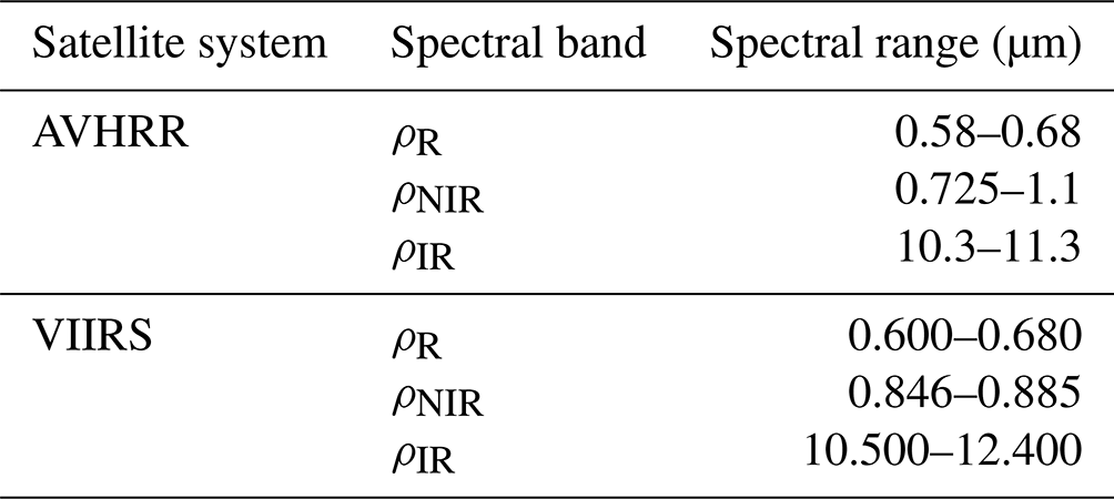
Satellite-based vegetation health products were obtained from NOAA.¹ The blended version (Yang et al., 2020) is composed of long-term remote sensing data derived from two systems of satellites: the AVHRR from 1981 to 2012 and its successor, the Visible Infrared Imaging Radiometer Suite (VIIRS), from 2013 onwards. The dataset includes two essential products, namely the NDVI and the BT (Table A3). The NDVI is computed from the red (ρ_R) and near-infrared (ρ_NIR) bands:

$$\begin{array}{}\text{(1)}& \text{NDVI}={\displaystyle \frac{({\mathit{\rho }}_{\mathrm{NIR}}-{\mathit{\rho }}_{\mathrm{R}})}{({\mathit{\rho }}_{\mathrm{NIR}}+{\mathit{\rho }}_{\mathrm{R}})}}.\end{array}$$

The NDVI is unitless and given in the range [−0.1, 1]. Same NDVI values should not be interpreted similarly for different ecosystems. In other words, the interpretation is highly dependent on the location and ecosystem productivity (Kogan, 1995b). The BT is derived from the infrared (ρ_IR) band and given in Kelvin (K) within the range [0, 400]. To handle high-frequency noise caused by clouds, aerosol, and atmospheric variation, along with different random error sources, the NDVI and BT were temporally aggregated into smoothed, noise-reduced weekly products. In addition, post-launch calibration coefficients and solar and sensor zenith angles are applied to account for sensor degradation and orbital drift. The outlier removal is essential for excluding invalid measurements. Additionally, this weekly temporal resolution is enough to capture the phenological phases of vegetation and is adequate for satellite data application (Kogan et al., 2011; Yang et al., 2020). Based on the NDVI, BT, and their long-term climatologies, the upper and lower bounds of the ecosystem (minimum and maximum values for the NDVI and BT) can be estimated. Hence, the VCI, TCI, and VHI can be derived pixel-wise (Kogan, 1995a, 1990). The vegetation condition index is given by

$$\begin{array}{}\text{(2)}& \begin{array}{rl}\text{VCI}& =\mathrm{100}{\displaystyle \frac{(\text{NDVI}-{\text{NDVI}}_{\min })}{({\text{NDVI}}_{\max }-{\text{NDVI}}_{\min })}},\\ & \text{with}\text{VCI}\in [\mathrm{0},\mathrm{100}],\end{array}\end{array}$$

where NDVI is the weekly noise-reduced NDVI and NDVI_min and NDVI_max are the multi-year weekly absolute minimum and maximum NDVI values, respectively. The thermal condition index is given by

$$\begin{array}{}\text{(3)}& \text{TCI}=\mathrm{100}{\displaystyle \frac{({\text{BT}}_{\max }-\text{BT})}{({\text{BT}}_{\max }-{\text{BT}}_{\min })}},\text{with}\text{TCI}\in [\mathrm{0},\mathrm{100}],\end{array}$$

where BT is the weekly noise-reduced BT and BT_min and BT_max are the multi-year weekly absolute minimum and maximum BT values, respectively. The vegetation health index is given by

$$\begin{array}{}\text{(4)}& \text{VHI}=\left(\mathit{\alpha }\right)\text{VCI}+(\mathrm{1}-\mathit{\alpha })\text{TCI},\text{with}\text{VHI}\in [\mathrm{0},\mathrm{100}],\end{array}$$

where α is a weighting coefficient. While VCI is a proxy for the moisture condition and its lower values reflect a water-related stress, TCI is a proxy for the thermal condition, and its lower values indicate a temperature- and wetness-related stress. The composite index VHI is a linear combination of the former two indices for approximating the vegetation health. VHI fluctuates annually between 0 (unfavorable condition) and 100 (favorable condition). The values of these indices above 100 and below 0 are clipped. The dataset is provided globally with ∼0.05° (∼4 km) spatial resolution mapped onto the Plate carrée projection. NOAA vegetation products have been broadly used for research and real-world applications. For a summary of the validation and studies that use this dataset for agricultural drought monitoring, we refer to Yang et al. (2020).

2.3 Preprocessing

In this section we describe the data preprocessing that is needed prior to applying DL. Overall the TSMP has 30 years of data (1989–2019). We reserved the years 1989–2009 (AVHRR era) and 2013–2016 (VIIRS era) for training, 2010–2011 (AVHRR era) and 2017 (VIIRS era) for validation, and 2012 (AVHRR era) and 2018–2019 (VIIRS era) for testing. For the TSMP, we excluded the lateral boundary relaxation zone by removing invalid grid points from the boundaries. This results in a final grid with 397×409 grid cells in the latitudinal and longitudinal direction, respectively. In order to connect local-related characteristics to climate conditions, we computed three additional static variables from the static variables described in Table A2. We computed slope (Horn, 1981) and roughness (Wilson et al., 2007) from orography and distance to water from the land–sea mask. Due to the fact that the remote sensing data were obtained from two different satellite systems, the data derived from the VIIRS have to be first adjusted to insure continuity and consistency with the data derived from the AVHRR. Yang et al. (2018, 2021b) showed that the discrepancy between sensors are mainly due to the differences in spectral response ranges and calibration parameters. Compared to the BT/TCI, this has a greater impact on the NDVI/VCI (Kogan et al., 2015). Considering this issue, we followed the same re-compositing approach as described in Yang et al. (2021b). The re-compositing approach can be used to generate cross-sensor vegetation products for the time period from 2013 to 2019. In fact, the NDVI/BT from different sensors can be decomposed into climatologies and VCI and TCI. The climatology provides information about the ecosystem, and it is sensor-specific, while the VCI/TCI for the same ecosystem location are cross-sensor. Thus, using climatology from the AVHRR and VCI from the VIIRS, Eq. (2) can be reformulated to re-composite NDVI for the AVHRR as follows:

$$\begin{array}{}\text{(5)}& \begin{array}{rl}& {\text{NDVI}}_{\left(\mathrm{AVHRR}\right)}^{\prime }=\left({\displaystyle \frac{{\text{VCI}}_{\left(\mathrm{VIIRS}\right)}}{\mathrm{100}}}\right)({\text{NDVI}}_{(\max ,\mathrm{AVHRR})}\\ & -{\text{NDVI}}_{(\min ,\mathrm{AVHRR})})+{\text{NDVI}}_{(\min ,\mathrm{AVHRR})},\end{array}\end{array}$$

where ${\text{NDVI}}_{\left(\mathrm{AVHRR}\right)}^{\prime }$ is the converted weekly noise-reduced NDVI from the VIIRS to the AVHRR; VCI_(VIIRS) is the vegetation condition index derived from the VIIRS; and NDVI_(min,AVHRR) and NDVI_(max,AVHRR) are the multi-year weekly absolute minimum and maximum NDVI values (climatology) derived from the AVHRR, respectively. Similarly, from Eq. (3) we have

$$\begin{array}{}\text{(6)}& \begin{array}{rl}& {\text{BT}}_{\left(\mathrm{AVHRR}\right)}^{\prime }={\text{BT}}_{(\max ,\mathrm{AVHRR})}\\ & -\left({\displaystyle \frac{{\text{TCI}}_{\left(\mathrm{VIIRS}\right)}}{\mathrm{100}}}\right)({\text{BT}}_{(\max ,\mathrm{AVHRR})}-{\text{BT}}_{(\min ,\mathrm{AVHRR})}),\end{array}\end{array}$$

where ${\text{BT}}_{\left(\mathrm{AVHRR}\right)}^{\prime }$ is the converted weekly noise-reduced BT from the VIIRS to the AVHRR; TCI_(VIIRS) is the thermal condition index derived from the VIIRS; and BT_(min,AVHRR) and BT_(max,AVHRR) are the multi-year weekly absolute minimum and maximum BT values (climatology) derived from the AVHRR, respectively. Please note that VCI_(VIIRS) and TCI_(VIIRS) were based on a long-term pseudo-VIIRS climatology (for more details on this, please see Yang et al., 2018). In addition, the TSMP simulation and target remote sensing data have to be spatially aligned in the same domain. After the continuity at the NDVI and BT levels was realized, we mapped these two products onto the TSMP rotated coordinate system over the EURO-CORDEX EUR-11 domain. For the mapping, we upscaled the data from 0.05 to 0.11° resolution based on a first-order conservative mapping (Jones, 1999) using the package from Zhuang et al. (2020). For calculating the spatial mean, we excluded invalid, water, and coastal lines pixels. Afterwards, we computed the VCI, TCI and VHI based on Eqs. (2)–(4). We note that the weighted coefficient α in Eq. (4) can be empirically calibrated as a spatially variant factor (Zeng et al., 2022, 2023). Following previous works, we set α to its standard value of 0.5 in all experiments as in Yang et al. (2020). Furthermore, masks over desert and very cold areas were extracted from the quality assurance (QA) metadata provided with the data. Eventually, the preprocessed data were aggregated into data cubes ({variable, lat, lon}) on a weekly basis and stored as netCDF files. This remote sensing dataset can serve as a reference to train and evaluate the DL model performance. Overall, this includes 1263, 156, and 139 samples (weeks) for training, validation, and testing, respectively. To avoid overfitting or the dominance of a few input variables, we normalized the input of the TSMP by subtracting the mean and dividing by the standard deviation corresponding to each input variable. These statistics were computed only from the years that are used for training. The invalid values of pixels were replaced with zero values as input to the DL model.

3 Methodology

Given $\text{TSMP}\in {\mathbb{R}}^{V\times T\times W\times H}$ as a climate change simulation, where V is the number of output variables from the COSMO, CLM, and ParFlow models and the static forcing variables; T is the temporal dimension; and W and H are the spatial extensions, our objective is to construct a mapping function to predict $\text{NDVI}\in {\mathbb{R}}^{I\times W\times H}$ and $\text{BT}\in {\mathbb{R}}^{I\times W\times H}$ on a weekly basis, where I is the number of weeks. To accomplish this, we propose to approximate this function as a function f using a DL model based on a U-Net (Ronneberger et al., 2015) with focal modulations (Yang et al., 2022) as building blocks:

$$\begin{array}{}\text{(7)}& f:(\text{TSMP};\mathit{\theta })\to (\text{NDVI},\text{BT}),\end{array}$$

where θ is the weight of the model. The input for DL is a data cube representing a specific week i of TSMP data, and the output is the NDVI and BT corresponding to the same week i. We denote the weekly averaged input data cube produced by the TSMP as ${\mathbf{X}}^i\in {\mathbb{R}}^{V\times W\times H}$, where we obtain Xⁱ by taking the mean of the days corresponding to the week i. For simplicity, we will drop the notation i in the following sections. Firstly, the network architecture is introduced in Sect. 3.1, and the focal modulation is then described in Sect. 3.2. Section 3.3 discusses the loss function, and Sect. 3.4 outlines the baseline approaches. Implementation and technical details are given in Sect. 3.5. Finally, the evaluation metrics are described Sect. 3.6.

Figure 1 An overview of the proposed model for predicting the NDVI and BT from a TSMP climate simulation. The model follows the U-Net shape with encoder and decoder layers. We use focal modulation as the basic building block for the model. The input TSMP simulation is first encoded into a latent representation via encoder layers. In a subsequent step, the decoder constructs new features to be given as input to two separated regression heads that output the NDVI and BT simultaneously. The predicted NDVI and BT can then be used to derive different agricultural drought indices such as the VCI, TCI, and VHI.

3.1 Model architecture

The recent applications of vision transformers (ViTs) have covered many tasks in the field of computer vision. The network design of ViTs, along with the multi-head self-attention mechanism (Vaswani et al., 2017), allows ViTs to stand as the state-of-the-art backbone in recent DL models. In contrast to CNNs, ViTs with self-attention modules can handle long-range interactions across tokens (pixels) more efficiently. In a nutshell, the self-attention module aims to transfer pixel representations of a given image into a new feature representation based on a weighted aggregation of interactions between every individual pixel and its surrounding. This mechanism allows the model to focus on more relevant regions of the input images. Despite this powerful transforming process, the computational requirement of a standard ViT has been a limitation when applying it to vision tasks. More recently, the focal modulation network (Yang et al., 2022) has been introduced to substitute the self-attention mechanism with a lightweight focal module. In contrast to self-attention, focal modulation starts with contextual aggregation and ends with interactions. Based on this recently introduced mechanism, DL models were developed for medical image segmentation (Naderi et al., 2022; Rasoulian et al., 2023), change detection for remote sensing data (Fazry et al., 2023), and video action recognition (Wasim et al., 2023). We build our model on focal modulation networks and extend their applications in geoscience. Figure 1 provides an overview of the model architecture. The model design follows the U-Net shape with encoder and decoder layers connected via skip connections and followed by two regression heads. This allows the model to extract features in a hierarchical way and predict the NDVI and BT with customized heads. In the following, we describe the main parts of the model:

• Patch embedding. The patch embedding is implemented as a single 1D convolution, where one patch is equivalent to one pixel. The role of this embedding is to project the input X from V dimension into a channel dimension that matches the channel dimension C_(en,1) of the first encoder block. In contrast to related works with transformers, we do not reduce the spatial resolution at this step. This is important for mitigating blurring effects in regression tasks. An analysis of the impact of the patch size for embedding is provided in Appendix E.

• Encoder. The encoder consists of three encoding layers. Each layer has two consecutive focal modulation blocks that have the same number of channels. We use focal modulation to capture local to global dependencies in the domain (Sect. 3.2). We apply down-sampling to the output of the first two encoder layers to reduce the spatial resolution by a factor of 2 and double the number of channels. The down-sampling is implemented as a 2D convolution with a 2×2 kernel size and a stride of 2. We set $C_{(\mathrm{en},\mathrm{1})}=\mathrm{96}$ as the number of channels of the first encoder layer. Consequently, the encoder has the dimensionality {$C_{(\mathrm{en},\mathrm{1})}=\mathrm{96},C_{(\mathrm{en},\mathrm{2})}=\mathrm{192},C_{(\mathrm{en},\mathrm{3})}=\mathrm{384}$}, where C_(en,2) is the dimensionality for the second encoder layer and C_(en,3) is the dimensionality for the third encoder layer. The encoder allows the network to extract low- to high-level features in a hierarchical way. Note that focal modulation allows an additional hierarchical feature extraction at each level (Sect. 3.2).

• Skip connections. These connections copy outputs from each encoder layer into its corresponding decoder layer. The purpose of this is to enhance the gradient flow in the network and to prevent vanishing gradient issues.

• Decoder. The decoder has a similar design to the encoder. It consists of three decoder layers with two consecutive focal modulation blocks for each decoder layer. The input for the first decoder layer is the output of the last encoder layer copied via a skip connection. The input for the second and third decoder layers is a concatenation of the output from the previous decoder layer with the output of the corresponding encoder layer. The outputs of the first and second decoder layers are up-sampled to double the image size and to reduce the dimensionality by a factor of 2. The up-sampling is implemented as a bilinear interpolation followed by a 2D convolution with a 1×1 kernel size and a stride of 1. The decoder layers have the dimensionality {$C_{(\mathrm{de},\mathrm{1})}=C_{(\mathrm{en},\mathrm{3})}=\mathrm{384},C_{(\mathrm{de},\mathrm{2})}=C_{(\mathrm{en},\mathrm{2})}+C_{(\mathrm{de},\mathrm{1})}=\mathrm{384},C_{(\mathrm{de},\mathrm{3})}=C_{(\mathrm{en},\mathrm{1})}+C_{(\mathrm{de},\mathrm{2})}=\mathrm{288}$}, where C_(de,1), C_(de,2), and C_(de,3) are the dimensionality for the first, second, and third decoder layers, respectively. The purpose of the decoder is to gradually construct the input for the regression heads from the encoded features.

• Regression heads. The output of the last decoder layer is then given as input to two separated regression heads to predict the NDVI and BT. Each head has two 2D convolutions with a 3×3 kernel size and a stride of 1 with a LeakyReLU activation in between. The regression head reduces the dimensionality from $C_{(\mathrm{de},\mathrm{3})}=\mathrm{288}$ to 128 and then to 1.

3.2 Focal modulations

We first describe how the block is implemented and then describe the main focal modulation module denoted as FM. Figure 2 illustrates the architecture of the focal modulation block used in both the encoder and decoder layers. The design follows a typical transformer block. Let ${\mathbf{X}}^k\in {\mathbb{R}}^{N\times C^k\times W^k\times H^k}$ be the input at the kth block, where N is the batch size (number of input tensors), C^k is the number of input channels, and W^k and H^k are the spatial resolution. Firstly, the input is normalized across N via a layer normalization (Ba et al., 2016) denoted as LayerNorm. Using the indices $n\in \mathit{\{}\mathrm{1},\mathrm{\dots },N\mathit{\}}$, $c^k\in \mathit{\{}\mathrm{1},\mathrm{\dots },C^k\mathit{\}}$, $w^k\in \mathit{\{}\mathrm{1},\mathrm{\dots },W^k\mathit{\}}$, and $h^k\in \mathit{\{}\mathrm{1},\mathrm{\dots },H^k\mathit{\}}$, the LayerNorm can be written as

$$\begin{array}{}\text{(8)}& {\displaystyle }\begin{array}{rl}\text{LayerNorm}({\mathbf{X}}^k;({\mathit{\gamma }}_l^k,{\mathit{\beta }}_l^k\left)\right)& =\left({\displaystyle \frac{{{\mathbf{X}}_n^k}_{(c^k,w^k,h^k)}-{\mathit{\mu }}_n^k}{{\mathit{\sigma }}_n^k}}\right)\\ & \cdot {{\mathit{\gamma }}_l^k}_{\left(c^k\right)}+{{\mathit{\beta }}_l^k}_{\left(c^k\right)},\end{array}\text{(9)}& {\displaystyle }{\mathit{\mu }}_n^k={\displaystyle \frac{\mathrm{1}}{C^k{W}^k{H}^k}}\sum _{c^k=\mathrm{1}}^{C^k}\sum _{w^k=\mathrm{1}}^{W^k}\sum _{h^k=\mathrm{1}}^{H^k}{{\mathbf{X}}_n^k}_{(c^k,w^k,h^k)},\text{(10)}& {\displaystyle }{\mathit{\sigma }}_n^k=\sqrt{{\displaystyle \frac{\mathrm{1}}{C^k{W}^k{H}^k}}\sum _{c^k=\mathrm{1}}^{C^k}\sum _{w^k=\mathrm{1}}^{W^k}\sum _{h^k=\mathrm{1}}^{H^k}({{\mathbf{X}}_n^k}_{(c^k,w^k,h^k)}-{\mathit{\mu }}_n^k{)}^{\mathrm{2}}},\end{array}$$

where ${{\mathbf{X}}_n^k}_{(c^k,w^k,h^k)}$ is the input tensor of order n in the batch, ${\mathit{\mu }}_n^k$ and ${\mathit{\sigma }}_n^k$ are the computed mean and standard deviation of the corresponding input ${{\mathbf{X}}_n^k}_{(c^k,w^k,h^k)}$, and ${{\mathit{\gamma }}_l^k}_{\left(c^k\right)}\in {\mathbb{R}}^{C^k}$ and ${{\mathit{\beta }}_l^k}_{\left(c^k\right)}\in {\mathbb{R}}^{C^k}$ are per-channel learnable parameters.

Figure 2 An illustration of the focal modulation block. It follows the typical transformer block with a focal modulation instead of self-attention. X^k represents the input to the kth block.

These learnable parameters are shared across input tensors. The output of LayerNorm is then passed into the function FM. After that, the output of the first part is normalized by a second LayerNorm and passed into a feed-forward layer (FFL). The FFL consists of one linear layer that maps the dimensionality to r_mlp×C^k followed by a GELU activation (Hendrycks and Gimpel, 2016) and a second linear layer to bring the dimensionality back to C^k, where r_mlp is the MLP ratio parameter. We set r_mlp to 4 for the encoder and decrease it to 2 for the decoder to reduce the number of model parameters. The output of each block can be formulated as follows:

$$\begin{array}{}\text{(11)}& \begin{array}{rl}& \text{FocalModulationBlock}\left({\mathbf{X}}^k\right)\triangleq {\mathit{\gamma }}_{\mathrm{2}}^k\\ & \left(\text{FFL}\right(\text{LayerNorm}\left({\mathit{\gamma }}_{\mathrm{1}}^k\text{FM}\right(\text{LayerNorm}\left({\mathbf{X}}^k\right))+{\mathbf{X}}^k)\left)\right)\\ & +\left({\mathit{\gamma }}_{\mathrm{1}}^k\text{FM}\right(\text{LayerNorm}\left({\mathbf{X}}^k\right))+{\mathbf{X}}^k)),\end{array}\end{array}$$

where ${\mathit{\gamma }}_{\mathrm{1}}^k\in {\mathbb{R}}^{C^k}$ and ${\mathit{\gamma }}_{\mathrm{2}}^k\in {\mathbb{R}}^{C^k}$ are learnable scaling parameters. The main component of each focal modulation block is the FM function. As seen in Fig. 3, it consists of three main steps: hierarchical contextualization, gated aggregation, and interactions.

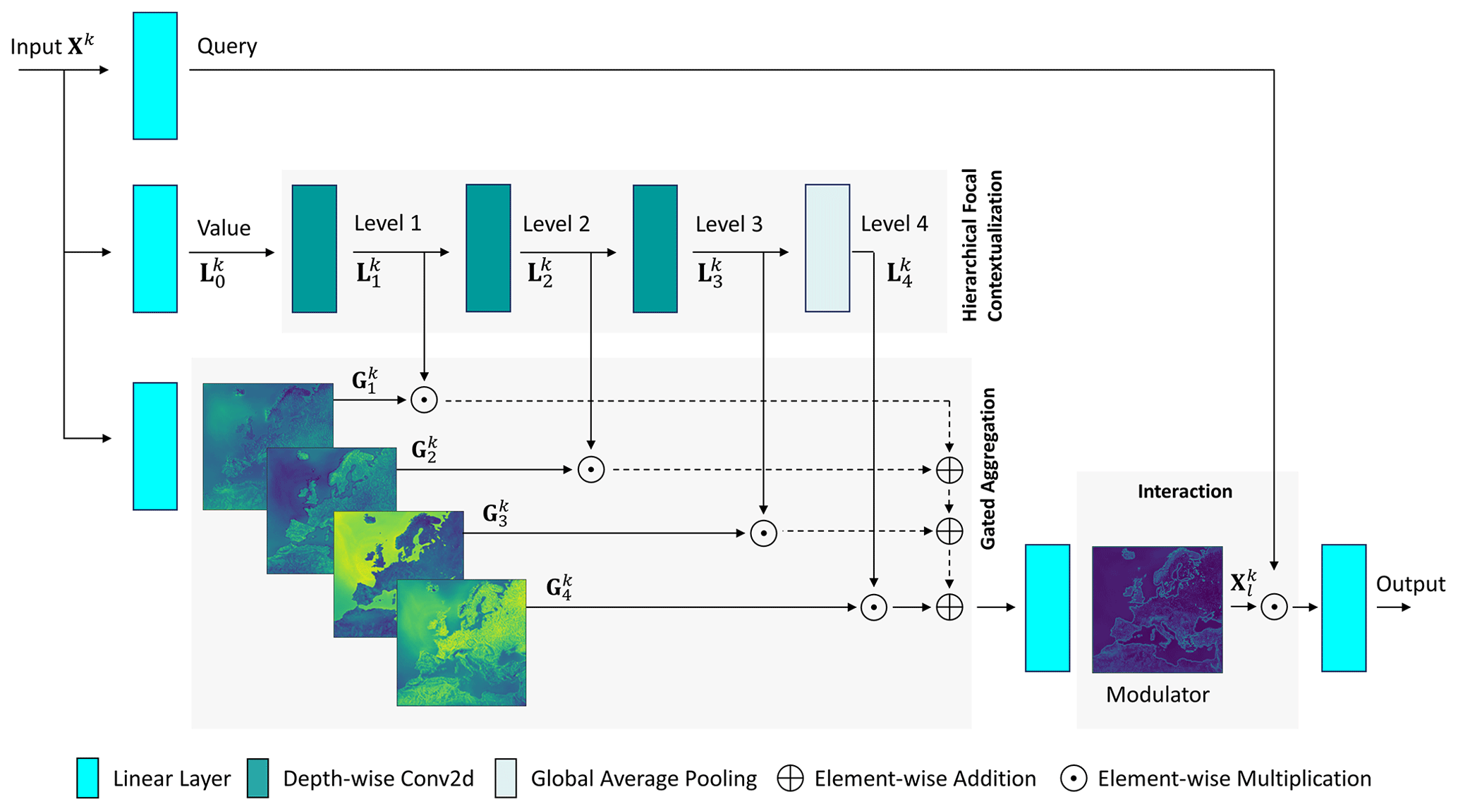
Figure 3 An illustration of the function FM at kth block. It consists of three main parts: focal contextualization, gated aggregation, and interaction. Firstly, the query, value, and gates are obtained by projecting X^k with linear layers. Then, a stack of depth-wise 2D convolutions followed by a global pooling is used on the value to derive contextual features around pixels. Gates are used to adaptive aggregate contextual features into a modulator. Finally, the interaction between queried pixels and the modulator is performed and projected by a final linear layer to compute the output. The shown images are examples of learned gates along with the pixel-wise magnitude of the corresponding modulator at the first block encoder. The bright colors (i.e., green to yellow) for specific regions represent higher values which correspond to higher attentions of the model to that regions.

• Hierarchical contextualization. The objective of this part is to encode local to global range dependencies for every pixel. It is based on Focal Transformer (Yang et al., 2021a) and aims to extract features at four different levels. Let X^k be the input for FM and L=4 be the number of levels. Firstly, X^k is projected by a linear layer into a new representation ${\mathbf{L}}_{\mathrm{0}}^k=\text{Linear}\left({\mathbf{X}}^k\right)\in {\mathbb{R}}^{N\times C^k\times W^k\times H^k}$. Afterwards, the contexts are obtained in a recursive manner using a sequence of three depth-wise 2D convolutions (DWConv2D) with GELU activation and with increased receptive fields. In DWConv2D, each output channel corresponds to a convolution on one input channel. We denote r_l as the kernel size at level l and start with r₁=3. Thereby, the kernel sizes at the focal levels have the values r₁=3, r₂=5, and r₃=7. To obtain a global feature representation, a global average pooling (GAP) followed by a GELU activation is applied at level l=4. Using the index $l\in \mathit{\{}\mathrm{1},\mathrm{\dots },L\mathit{\}}$, the hierarchical contextualization can be formulated as follows:

  $$\begin{array}{}\text{(12)}& {\mathbf{L}}_l^k\triangleq \left\{\begin{array}{ll}\text{GELU}\left(\text{DWConv2D}\right({\mathbf{L}}_{l-\mathrm{1}}^k\left)\right),& \text{if}\mathrm{1}\le l<L,\\ \text{GELU}\left(\text{GAP}\right({\mathbf{L}}_{l-\mathrm{1}}^k\left)\right),& \text{otherwise.}\end{array}\right.\end{array}$$

• Gated aggregation. The gated aggregation adaptively summarizes the extracted hierarchical contexts ${\mathbf{L}}_l^k$ into a modulator. First, X^k is projected by a linear layer into four gates, ${\mathbf{G}}^k=\text{Linear}\left({\mathbf{X}}^k\right)\in {\mathbb{R}}^{N\times L\times W^k\times H^k}$. As can be seen from the example in Fig. 3, the third gate focuses on the water area while other gates focus on different segmented regions. This allows each pixel to adaptively aggregate features from different semantic regions conditioned on its context. Pixels in a less dynamic environment may depend on more distant pixels, while pixels in a more dynamic environment may depend more on the local context. The aggregation is performed over different focal levels and followed by a linear layer:

  $$\begin{array}{}\text{(13)}& {\mathbf{X}}_L^k\triangleq \text{Linear}\left(\sum _{l=\mathrm{1}}^L{\mathbf{G}}_l^k\odot {\mathbf{L}}_l^k\right),\end{array}$$

  where ${\mathbf{X}}_L^k\in {\mathbb{R}}^{N\times C^k\times W^k\times H^k}$ are the contextual aggregated features for each pixel called the modulator, ${\mathbf{G}}_l^k$ is the gate corresponding to level l, and ⊙ is the Hadamard operator (element-wise multiplication).

• Interaction. Finally, the interaction between the queried pixels and the modulator is given with the following formula:

  $$\begin{array}{}\text{(14)}& \text{FM}\left({\mathbf{X}}^k\right)\triangleq {\mathbf{X}}_L^k\odot \text{Linear}\left({\mathbf{X}}^k\right)\in {\mathbb{R}}^{N\times C^k\times W^k\times H^k}.\end{array}$$

3.3 Loss function

For training we use the mean absolute error (MAE) as a loss function, since it is less sensitive to outliers than the mean squared error (MSE):

$$\begin{array}{}\text{(15)}& {\mathcal{L}}_{\mathrm{MAE}}={\displaystyle \frac{\mathrm{1}}{NWH}}\sum _{n=\mathrm{1}}^N\sum _{w=\mathrm{1}}^W\sum _{h=\mathrm{1}}^H|{\mathbf{Y}}_{(n,w,h)}-{\widehat{\mathbf{Y}}}_{(n,w,h)}|,\end{array}$$

where N is the batch size and ${\mathbf{Y}}_{(n,w,h)}$ and ${\widehat{\mathbf{Y}}}_{(n,w,h)}$ are the predicted and observed images, respectively.

In addition, to increase local variability and balance the blurring effects from Eq. (15), we use a perceptual loss (Ledig et al., 2017; Johnson et al., 2016) based on a pre-trained VGG-19 network (Simonyan and Zisserman, 2014) on ImageNet (Deng et al., 2009). This additional loss constrains the generated images to have a similar structure and spatial variability to the observed images by comparing multi-level features extracted by a VGG classifier network from both the predicted and observed images:

$$\begin{array}{}\text{(16)}& {\displaystyle }{\mathcal{L}}_{\mathrm{VGG}}=\mathrm{8}{\mathcal{L}}_{\mathrm{VGG}}^{\mathrm{1}}+\sum _{j=\mathrm{2}}^J{\mathcal{L}}_{\mathrm{VGG}}^j,\text{(17)}& {\displaystyle }\begin{array}{rl}& {\mathcal{L}}_{\mathrm{VGG}}^j={\displaystyle \frac{\mathrm{1}}{N{C}^j{W}^j{H}^j}}\sum _{n=\mathrm{1}}^N\sum _{c=\mathrm{1}}^{C^j}\sum _{w=\mathrm{1}}^{W^j}\sum _{h=\mathrm{1}}^{H^j}\\ & \left|{\mathit{\varphi }}^j\right({\mathbf{Y}}_{(n,j,c,w,h,)})-{\mathit{\varphi }}^j({\widehat{\mathbf{Y}}}_{(n,j,c,w,h)}\left)\right|,\end{array}\end{array}$$

where J is the number of levels from which the VGG features are extracted; W^j and H^j are the spatial extensions of the respective level within the VGG classifier; C^j is the number of the channel dimension of the respective level; and ${\mathit{\varphi }}^j\left({\mathbf{Y}}_{(n,j,c,w,h,)}\right)$ and ${\mathit{\varphi }}^j\left({\widehat{\mathbf{Y}}}_{(n,j,c,w,h,)}\right)$ are the extracted features at level j from the predicted and observed images, respectively. In contrast to classification problems where high-level features play a more important role, we multiply the low-level features by a weighting factor of 8 to preserve the local features and give them more importance since these are more relevant to our regression task. The VGG network was originally trained with RGB images, and giving the NDVI and BT as input is not directly possible. To solve this issue, we replicate the NDVI and BT along the channel dimension and feed each of them separately to the VGG network. The impact of using this perceptual loss is evaluated in Appendix D. The entire loss function to be minimized is thus given as follows:

$$\begin{array}{}\text{(18)}& \mathcal{L}={\mathcal{L}}_{\mathrm{MAE}}^{\mathrm{NDVI}}+\mathrm{0.1}{\mathcal{L}}_{\mathrm{VGG}}^{\mathrm{NDVI}}+{\mathcal{L}}_{\mathrm{MAE}}^{\mathrm{BT}}+\mathrm{0.1}{\mathcal{L}}_{\mathrm{VGG}}^{\mathrm{BT}},\end{array}$$

where ${\mathcal{L}}_{\mathrm{MAE}}^{\mathrm{NDVI}}$ and ${\mathcal{L}}_{\mathrm{VGG}}^{\mathrm{NDVI}}$ are the MAE and VGG losses on the NDVI and ${\mathcal{L}}_{\mathrm{MAE}}^{\mathrm{BT}}$ and ${\mathcal{L}}_{\mathrm{VGG}}^{\mathrm{BT}}$ are the MAE and VGG losses on BT, respectively. The weighting factor of 0.1 is set to balance the losses. The model is trained with a stochastic gradient descent. More technical details regarding the training are provided in Sect. 3.5.

3.4 Baseline approaches

We study the performance of recently developed vision transformers on our task. We achieve this by sharing the overall model architecture and implementing the main building block inside the encoder and decoder according to different algorithms. The implemented models are as follows:

• U-Net (Ronneberger et al., 2015) serves as a baseline of typical U-Net models. We implemented this model based on a 2D CNN with residual convolutional blocks. The U-Net model does not use an attention mechanism.

• Swin Transformer V1 (Liu et al., 2021) performs self-attention in shifted windows to reduce the computational complexity compared to the original ViT. Transformers based on this model have been commonly applied for a variety of tasks in remote sensing and computer vision (Wang et al., 2022a; Gao et al., 2021; Wang et al., 2022b; Aleissaee et al., 2023).

  Swin Transformer V2 (Liu et al., 2022) is an improved model of Swin V1. The attention mechanism is replaced with a scaled cosine attention to measure pixel feature similarities. Swin V2 utilizes post-normalization layers inside the main block, thus making the optimization of large models more stable. In addition, it proposes to replace the positional encoding inside the windows with a log-spaced continuous one to ease downstream tasks with pre-trained models.

• Wave-MLP (Tang et al., 2022) is a MLP-Mixer-based transformer model. The basic block is built on a stack of MLPs. Wave-MLP represents each pixel as a wave function with amplitude features representing pixel contents and phase to measure the relations with other pixels.

Apart from these models, we report the results for two NDVI and BT climatology baselines. The climatology is based on multi-year mean values computed from remote sensing observations pixel-wise and on a weekly basis. The first is climatology-I computed from the years 1981–1988 which represents a prescribed satellite phenology before the beginning of the simulation. The second is climatology-II computed from the training years 1989–2016 in an overlap with the simulation period. The later climatology represents a function that models the annual cycles, and it can be used to check if the models generalize beyond the mean annual cycles of the predicted NDVI or BT.

3.5 Implementation details

We re-implemented all aforementioned DL models in our framework and trained them with three different random seeds, which ensures a fair comparison and better estimation. All models have almost the same capacity with ∼12 million parameters. The encoders for the transformer models were pre-trained on ImageNet-1K (Deng et al., 2009), while the weights in the decoders and regression heads were initialized randomly from a standard normal distribution. To increase the generalization and robustness of the models, we use four augmentation techniques. This includes flipping and rotating the input with a probability of 0.5 and randomly perturbing the input variables by adding noise from a normal distribution with zero mean and a standard deviation of 0.02 with a probability of 0.5. In addition, to generate the input corresponding to week i during training, we randomly average two days corresponding to the week i as an additional augmentation technique. All models were trained with the ℒ loss Eq. (18) using the PyTorch framework (Paszke et al., 2019) with a learning rate of 0.0003 and a scheduler to decay the learning rate by a factor of 0.9 every 16 epochs. The AdamW optimizer (Loshchilov and Hutter, 2019) was used for the gradient descent with (${\mathit{\beta }}_{\mathrm{1}}=\mathrm{0.9},{\mathit{\beta }}_{\mathrm{2}}=\mathrm{0.999}$) and a weight decay of 0.05. We use a dropout probability of 0.2 and a stochastic depth rate of 0.3. We train with a batch size of N=2 for 100 epochs. For Swin Transformers, we set the window size to 8 and use the following number of heads $\mathit{\{}\mathrm{3},\mathrm{6},\mathrm{12}\mathit{\}}$ for the encoder and the same order for the decoder. The down-sampling in the encoder followed the original implementation in Swin Transformer. Wave-MLP was trained with the dimensionality {$C_{(\mathrm{en},\mathrm{1})}=\mathrm{64},C_{(\mathrm{en},\mathrm{2})}=\mathrm{128},C_{(\mathrm{en},\mathrm{3})}=\mathrm{320}$} and r_mlp=4 for both the encoder and the decoder. Wave-MLP and Swin V2 use a dropout probability of 0.1 and a stochastic depth rate of 0.2. In addition, we follow the official implementation of Wave-MLP and use GroupNorm (Wu and He, 2018) with a group of 1 instead of LayerNorm. Finally, all models were trained on individual NVIDIA RTX A6000 GPUs with 48 GB.

3.6 Evaluation metrics

To measure the model performance, we use the mean absolute error (MAE), root-mean-square error (RMSE), coefficient of determination (R²), Pearson correlation coefficient (R_p), and Spearman correlation coefficient (R_s). In addition, we compute the bias as ($\text{predicted}-\text{observed}={\mathbf{Y}}_{(w,h)}-{\widehat{\mathbf{Y}}}_{(w,h)}$). We compute the metrics for each sample and then average the values to obtain the final metrics. The MAE is computed from Eq. (15), while the RMSE can be calculated as follows:

$$\begin{array}{}\text{(19)}& \begin{array}{rl}& \text{RMSE}({\mathbf{Y}}_{(w,h)},{\widehat{\mathbf{Y}}}_{(w,h)})=\\ & \sqrt{{\displaystyle \frac{\mathrm{1}}{WH}}\sum _{w=\mathrm{1}}^W\sum _{h=\mathrm{1}}^H({\mathbf{Y}}_{(w,h)}-{\widehat{\mathbf{Y}}}_{(w,h)}{)}^{\mathrm{2}}}.\end{array}\end{array}$$

R² measures the variation of the perdition from the regression-fitted line, and it is calculated as follows:

$$\begin{array}{}\text{(20)}& \begin{array}{rl}& R^{\mathrm{2}}({\mathbf{Y}}_{(w,h)},{\widehat{\mathbf{Y}}}_{(w,h)})=\\ & \mathrm{1}-{\displaystyle \frac{{\sum }_{w=\mathrm{1}}^W{\sum }_{h=\mathrm{1}}^H({\mathbf{Y}}_{(w,h)}-{\widehat{\mathbf{Y}}}_{(w,h)}{)}^{\mathrm{2}}}{{\sum }_{w=\mathrm{1}}^W{\sum }_{h=\mathrm{1}}^H({\mathbf{Y}}_{(w,h)}-\widehat{\overline{Y}}{)}^{\mathrm{2}}}},\end{array}\end{array}$$

where $\widehat{\overline{Y}}$ is the overall mean observed value. The highest value for R² is 1, which represents a perfect fit. Please note that R² measures the variability in ${\widehat{\mathbf{Y}}}_{(w,h)}$ predicted by the model; thus it is by definition inversely proportional to the variance and noise in the observations and should be interpreted carefully.

The Pearson correlation (R_p) is a parametric correlation that measures the linear correlation between the predicted and observed values:

$$\begin{array}{}\text{(21)}& \begin{array}{rl}& R_{\mathrm{p}}({\mathbf{Y}}_{(w,h)},{\widehat{\mathbf{Y}}}_{(w,h)})=\\ & {\displaystyle \frac{{\sum }_{w=\mathrm{1}}^W{\sum }_{h=\mathrm{1}}^H({\mathbf{Y}}_{(w,h)}-\overline{Y})({\widehat{\mathbf{Y}}}_{(w,h)}-\widehat{\overline{Y}})}{\sqrt{{\sum }_{w=\mathrm{1}}^W{\sum }_{h=\mathrm{1}}^H({\mathbf{Y}}_{(w,h)}-\overline{Y}{)}^{\mathrm{2}}}\sqrt{{\sum }_{w=\mathrm{1}}^W{\sum }_{h=\mathrm{1}}^H({\widehat{\mathbf{Y}}}_{(w,h)}-\widehat{\overline{Y}}{)}^{\mathrm{2}}}}},\end{array}\end{array}$$

where $\overline{Y}$ is the mean predicted value. The best value for R_p is 1, which represents a perfect positive correlation.

The Spearman correlation (R_s) is a non-parametric measure of the relationship between predicted and observed values that can be calculated as follows:

$$\begin{array}{}\text{(22)}& R_{\mathrm{s}}({\mathbf{Y}}_{(w,h)},{\widehat{\mathbf{Y}}}_{(w,h)})=R_{\mathrm{p}}\left(R\right({\mathbf{Y}}_{(w,h)}),R({\widehat{\mathbf{Y}}}_{(w,h)}\left)\right),\end{array}$$

where R(Y_(w,h)) and $R\left({\widehat{\mathbf{Y}}}_{(w,h)}\right)$ are ranks obtained from the predicted and observed values, respectively. A perfect positive correlation occurs when R_s is 1.

4 Experimental results and analysis

4.1 NDVI and BT prediction

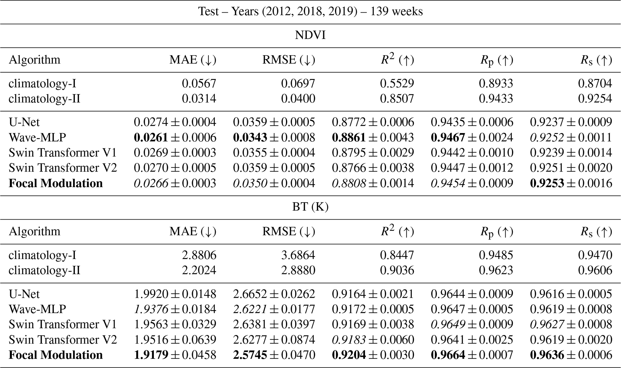
The quantitative results of the models are shown in Tables 1 and 2. Pixels without a vegetation cover (i.e., pixels over desert) were excluded from the results. Including these pixels will overestimate the model performance since they have small variations throughout the years. For the masking, we use NOAA quality assurance (QA) metadata. As can be seen in Tables 1 and 2, all DL models outperform the first climatology-I baseline by a huge margin. This is because the climatology was calculated before the simulation run. This climatology cannot capture the dynamic after 3 decades. The second climatology-II baseline is stronger. It uses information from multiple years within the simulation run. All DL models still achieve better results indicating that the models have learned the seasonal dynamic beyond climatology. In addition, these climatology baselines cannot be used to derive drought indices (Sect. 4.2) since the inter-annual variability in the NDVI and BT is neglected as average cycles are used. Furthermore, comparing the correlation and results of the BT with the NDVI, we can observe that all models achieve higher correlation metrics (R², R_p, and R_s) on the BT than on the NDVI. This can be explained by the fact that the NDVI is a composition of two bands while the BT is only derived from the infrared band; thus it is harder for the models to estimate the NDVI than the BT. In general, all DL models provide close results and are considered suitable for the task. Focal Modulation clearly outperformed other DL models on the validation set for both NDVI and BT predictions. For the test set on the NDVI, it comes slightly after the Wave-MLP model. However, Focal Modulation can generalize better for BT, thus providing a balanced prediction between the NDVI and BT, and consequently it is capable of generating an overall better prediction.

Table 1 Comparing the performance of different DL models. The metrics are shown for the validation set. The best and second-best results of each metric are highlighted in bold and italic text, respectively. (±) denotes the standard deviation for three different runs.

Table 2 Comparing the performance of different DL models. The metrics are shown for the test set. The best and second-best results of each metric are highlighted in bold and italic text, respectively. (±) denotes the standard deviation for three different runs.

In Table 3, we report the estimated inference time for the DL models. For the Focal Modulation model, the estimated inference time to generate one sample for the NDVI and BT containing $\mathrm{397}\times \mathrm{409}\times \mathrm{2}$ grid points is 0.24±0.01 s on one NVIDIA GeForce RTX 3090 GPU and 12±0.1 s on one AMD Ryzen 9 3900X 12-Core CPU. U-Net with a 2D CNN does not include operations for the attention mechanism; thus it is the fastest, but the performance is lower.

Table 3 Inference time in seconds for different DL models.

¹ NVIDIA GeForce RTX 3090 GPU, ² AMD Ryzen 9 3900X 12-Core CPU

Figure 4 Example predictions for the weekly NDVI from the test set. (a) Predicted NDVI. (b) Bias computed as prediction minus observed. (c) Distribution of biases. (d) Regression results as predicted versus observed. (e) Distribution of NDVI values for NOAA observation and model prediction. The metrics are computed over all pixels with vegetation cover.

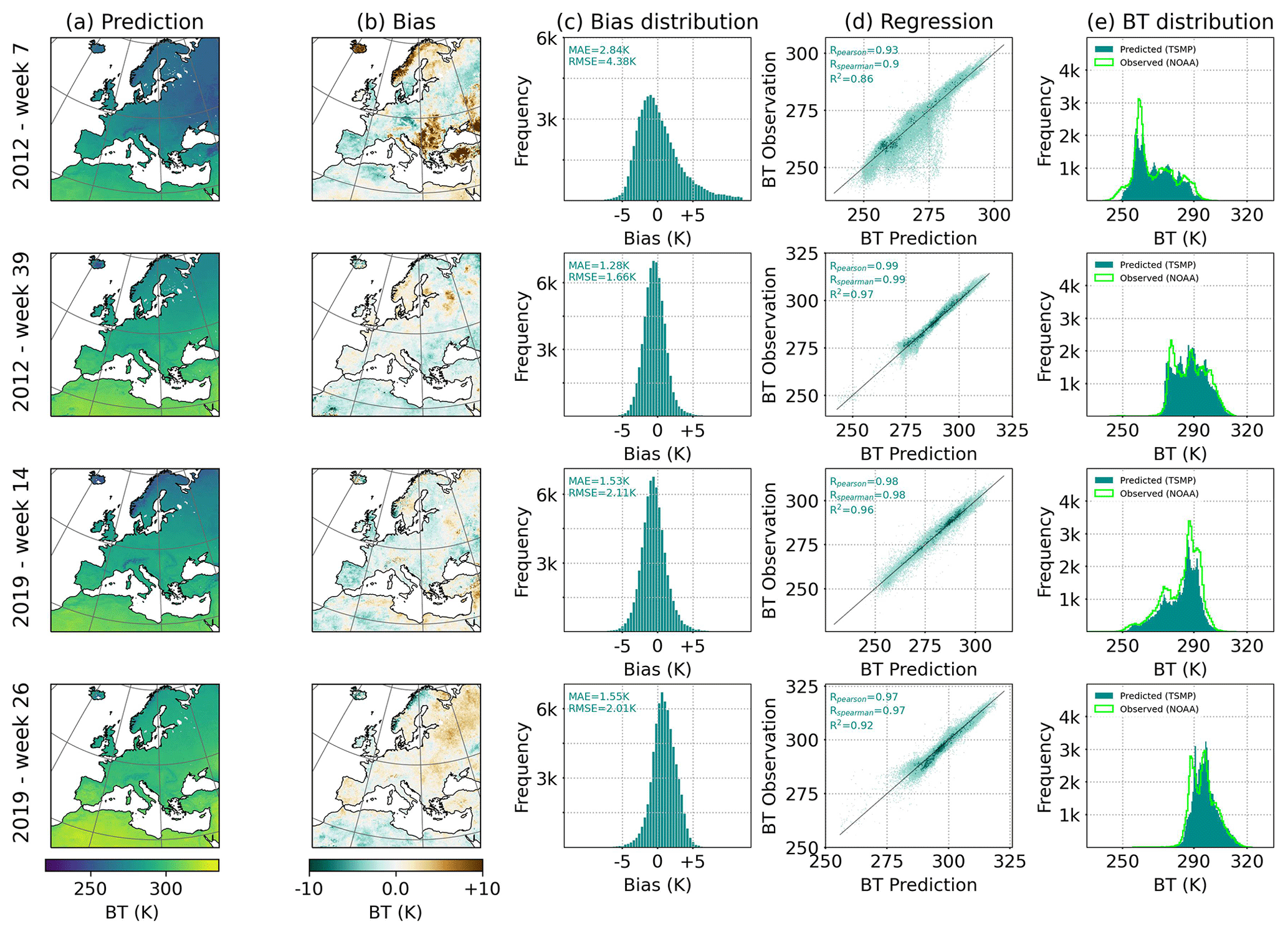
Figure 5 Example predictions for the weekly BT from the test set. (a) Predicted BT. (b) Bias computed as prediction minus observed. (c) Distribution of biases. (d) Regression results as predicted versus observed. (e) Distribution of BT values for NOAA observation and model prediction. The metrics are computed over all pixels with vegetation cover.

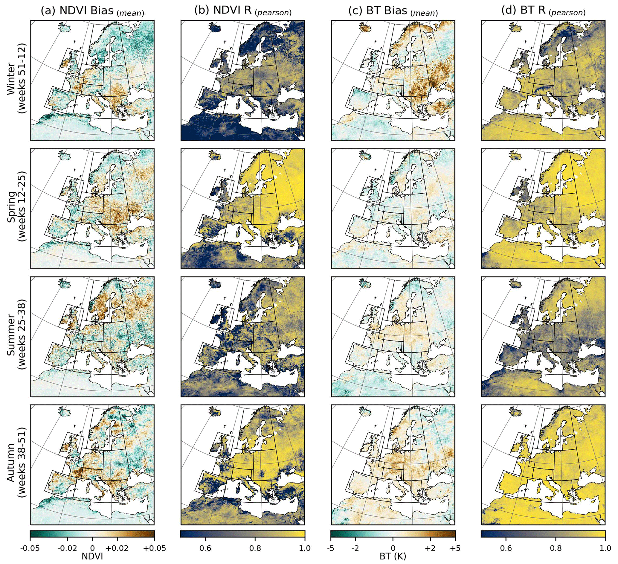
Figure 6 An analysis of uncertainty and model generalization for different times of the year. The analysis was performed on the validation and test sets as one set. (a) NDVI mean bias. (b) NDVI mean Pearson correlation. (c) BT mean bias. (d) BT mean Pearson correlation.

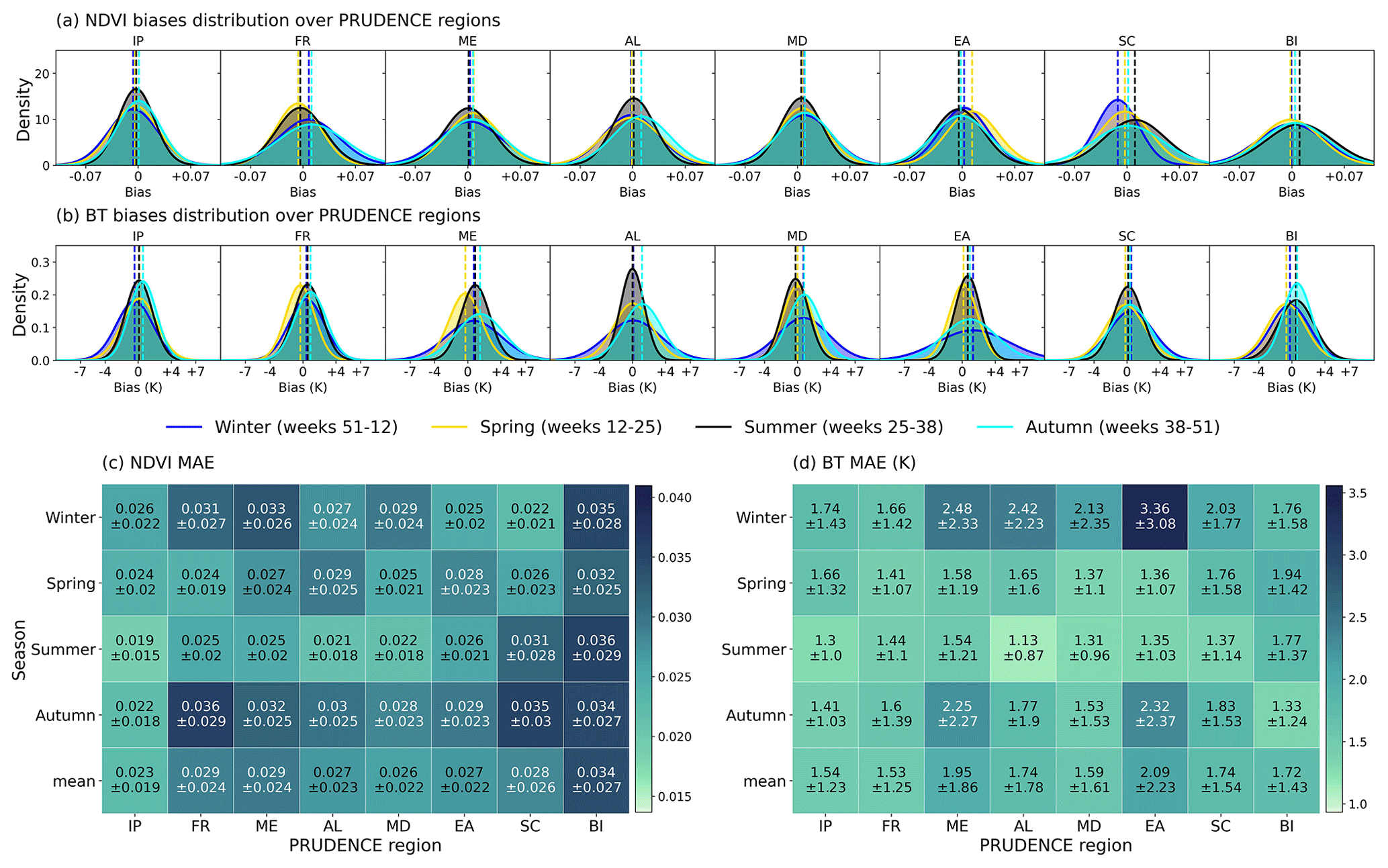
Figure 7 An analysis of uncertainty and model generalization for different times of the year over each PRUDENCE region. The analysis was performed on the validation and test sets as one set. (a) NDVI bias distribution. (b) BT bias distribution. Shown are the probability density functions. (c) NDVI MAE. (d) BT MAE.

Qualitative results for the model prediction with Focal Modulation are shown in Figs. 4 and 5. We take weeks from different seasons through the years and remove pixels over desert for the calculations of bias distribution and regression line. Positive bias values mean that the model overestimates the NDVI (BT) while negative ones indicate that the model underestimates the NDVI (BT). As shown in Figs. 4 and 5, the biases vary across the weeks and locations. For week 7 in 2012, the biases for both the NDVI and the BT are relatively high. Week 26 in 2019 exhibits similar high biases in both the NDVI and the BT over high-latitude regions. The respective distribution of biases is also shown in Figs. 4 and 5. Overall, the results show that the dynamics over the years are well captured. The biases for both the NDVI and the BT are closely centered around zero with a shift for the center of bias distribution from zeros. This shift is, however, in the same direction for both the NDVI and the BT. We can also observe that the model fits the regression lines better for weeks 14, 26, and 39 than for week 7 in winter 2012. The comparison between the distributions of predicted and observed NDVI/BT also confirms the observation that the model captured the dynamic throughout the years.

While this provides examples of the performance for individual samples, in Fig. 6 we provide an additional experiment where we analyze biases of model predictions in different seasons of the year and over PRUDENCE regions (see Fig. C1 in the Appendix for the definition of PRUDENCE regions). This allows us to assess the model weaknesses and strengths with different seasonality and spatial variability. The mean biases were computed pixel-wise from both the validation and test year time series, where we computed the biases for each pixel from the weeks that belong to a specific season and averaged the results to obtain the last metric. In addition, we computed the Pearson correlation R_p pixel-wise in a similar way. As seen in Fig. 6, there are clusters of positive and negative biases that vary with seasons over specific regions. For instance, for NDVI prediction, the eastern part of the British Isles exhibits positive biases for all seasons, while Iceland and northern Africa show constant negative biases. For BT, southeastern Europe has persistent positive biases with larger errors during winter. Pixels over desert, i.e., northern Africa, show less variability in the NDVI where only little seasonality is shown as in Fig. 4. Thus, such regions are easier to predict with relatively small biases. However, any fluctuation in the NDVI prediction over these pixels will lead to lower correlation compared to other regions, since the time series primarily represent small variations around the mean NDVI value. In comparison to other seasons, the winter season has relatively poor predictions, especially in the high-latitude regions. One possible explanation for these errors is the lack of accurate training data in Scandinavian regions during winter. For instance, previous studies on ParFlow-CLM models showed that hydrological modeling performs worse in northeastern Europe due to errors in snow dynamics and regional forces (Naz et al., 2023; Furusho-Percot et al., 2019a). It was also shown by Yang et al. (2020) and Eisfelder et al. (2023) that high-latitude regions are less reliable in deriving vegetation products due to snow cover and its effects on the albedo and larger sensor zenith angles. Another source of model errors is that NOAA vegetation products depend on temporal compositing to handle high frequency and atmosphere transmittance (Yang et al., 2020). The absence of a generalized physical-based model to enhance accuracy over various surfaces and for all conditions generates difficulties for satellite products (Kogan, 1995b). Nagol et al. (2009) assessed the uncertainty of the NDVI in this regard. These issues add some uncertainties to the model training and evaluation. Using more recent atmospheric correction methods such as in Moravec et al. (2021) could also enhance the results. Furthermore, as mentioned in Sect. 2.1, the TSMP simulation was performed in a free mode and had no modeling of anthropogenic-related influences. Given that agricultural systems and human activities which are interlinked with drought events could change and follow adaptation strategies (Van Loon et al., 2016), this certainly contributes to the error budget of the model. Developing realistic land use and water management scenarios within a probabilistic TSMP could reduce these errors. In addition, the uncertainty in the TSMP is highly linked to potential errors in the driving forces and spinup initialization. While these errors are common limitations of simulations and remote sensing data, it should be noted that the prediction of a DL model has its own uncertainty. Therefore, more efforts are needed to recognize the sources of uncertainty in model prediction (Sect. 4.2).

In Fig. 7, we visualize the computations over each PRUDENCE region separately. For Fig. 7a and b, we fit a normal distribution over the normalized histogram of biases for each season and over all PRUDENCE regions. For instance, positive shifts in the estimated means are shown in the NDVI for both FR and AL regions during autumn. The same pattern is shown for SC and BI during summer. As can also be seen in Fig. 7b, a positive shift in BT is shown for all regions during autumn. Furthermore, the shape of the distribution gives an overview of the prediction homogeneity within the region; i.e., the prediction is highly uncertain over EA during winter and consequently has a relatively high standard deviation. The mean values in Fig. 7c and d represent the expected MAE for all seasons combined. Figure 7c indicates that in general the model predictions for the NDVI are less certain during autumn in comparison to other periods and over BI within the PRUDENCE regions. For BT, it can be seen in Fig. 7d that the prediction is less certain during winter and over ME and EA regions.

4.2 Agricultural drought assessment

In this section, we assess the model's capability to predict different agricultural drought indices on a high temporal resolution (weekly basis). More specifically, we use the predicted NDVI and BT along with their multi-year climatology to derive the NDVI and BT anomalies and the VCI, TCI, and VHI drought indices. The NDVI and BT anomalies were computed by subtracting the mean value of the respective pixel and week from the predictions (observations). The VCI, TCI, and VHI were computed from Eqs. (2)–(4). Figures 8 and 9 compare the predicted agricultural drought indices VCI, TCI and VHI by the Focal Modulation model with the observed ones from NOAA remote sensing data for the years 2010–2012 (Fig. 8) and 2017–2019 (Fig. 9). We spatially average the values inside each PRUDENCE region and plot their respective time series on a weekly basis. Generally, values below 40 are identified as abnormally dry conditions (Kogan et al., 2015; Yang et al., 2020). Overall, the prediction resembles the seasonal wetness and dryness on a regional scale. The agreements between predictions and observations vary across regions and time with satisfactory R_p values ranging from 0.50 to 0.77, 0.38 to 0.70, and 0.50 to 0.75 for the VCI, TCI, and VHI, respectively. MAE values fluctuate in the ranges of 9.99–6.81, 13.88–10.24, and 5.80–2.69 for the VCI, TCI, and VHI, respectively. While there is a satisfactory agreement with observations, there are some obvious discrepancies, i.e., in the TCI over the Iberian Peninsula (IP) during summer 2018. More interestingly, we show the bounded results of an ensemble of DL models. This ensemble consists of the results of all DL models. As can be seen, all DL models which are based on different algorithms yield close predictions with small standard deviations. This supports the idea that errors in model prediction can probably be more attributed to biases in the TSMP model and remote sensing reference data. In this respect, Yang et al. (2021b) showed that vegetation products over regions with extremely little seasonality, i.e., desert and high mountains, have higher errors. This can be seen in Eqs. (2)–(4), where small differences between maximum and minimum values could lead to higher deviation in the vegetation indices.

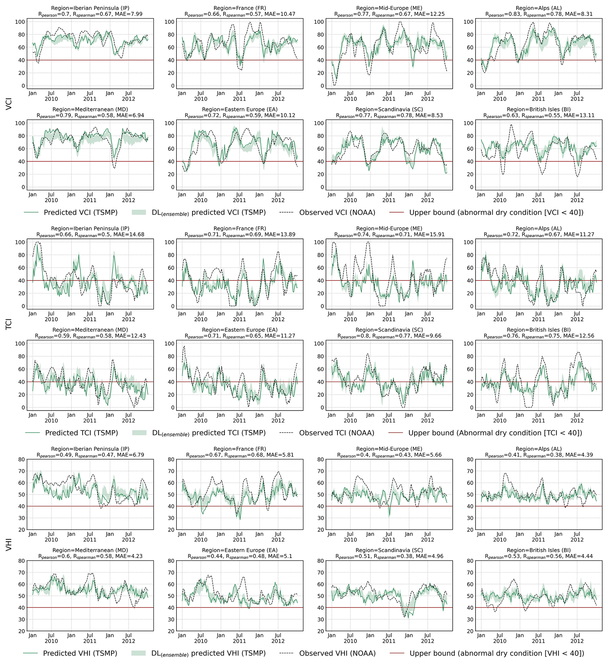
Figure 8 Comparison of spatially averaged weekly agricultural drought indices between the model prediction and NOAA observation over each PRUDENCE region. Drought indices were computed from the long-term climatology (1989–2016) pixel-wise and on a weekly basis. All results are obtained with the focal modulation network. The ensemble model is the result of all DL models described in Sect. 3. NDVI and BT anomalies are provided in Fig. F1 in the Appendix.

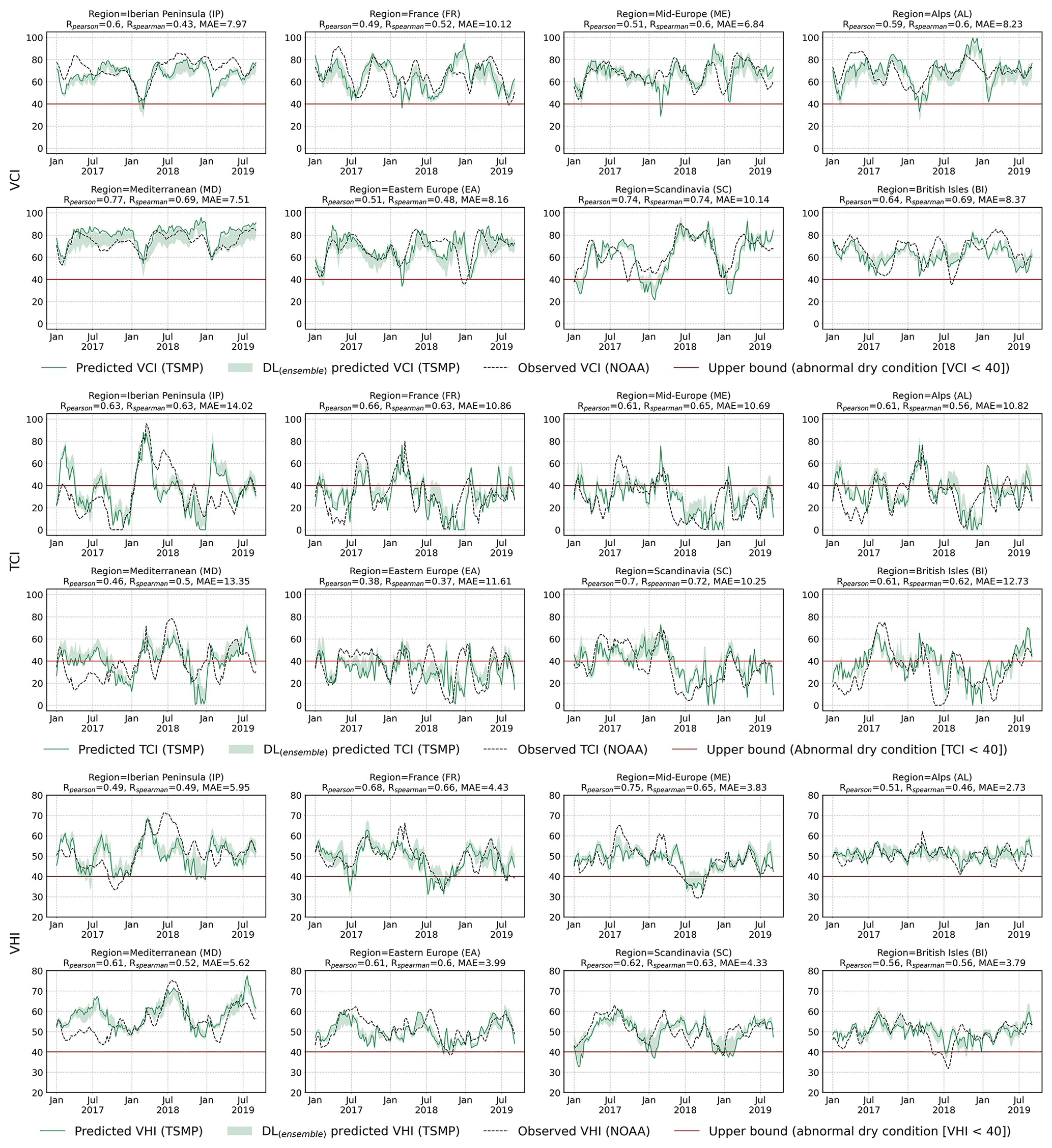
Figure 9 Comparison of spatially averaged weekly agricultural drought indices between the model prediction and NOAA observations over each PRUDENCE region. Drought indices were computed based on the long-term climatology (1989–2016) pixel-wise and on a weekly basis. All results are obtained with the focal modulation network. The ensemble model is the result of all DL models described in Sect. 3. NDVI and BT anomalies are provided in Fig. F2 in the Appendix.

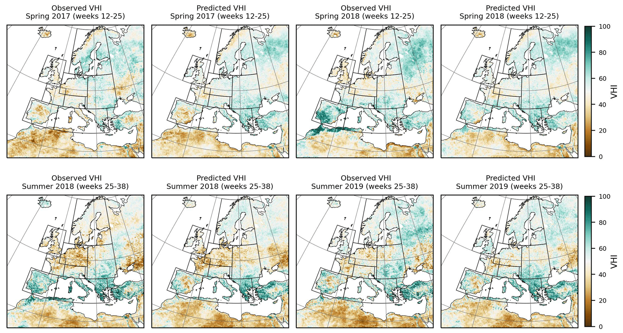
Figure 10 Comparison between the seasonal predicted vegetation health index (VHI) and NOAA observations over the pan-European domain.

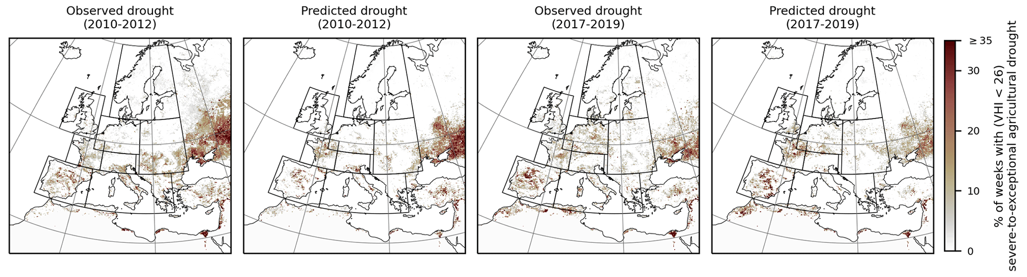
Figure 11 Comparison between the predicted drought frequency and NOAA observations over the pan-European domain. Frequency represents the percent of weeks with severe to exceptional drought events (VHI < 26).

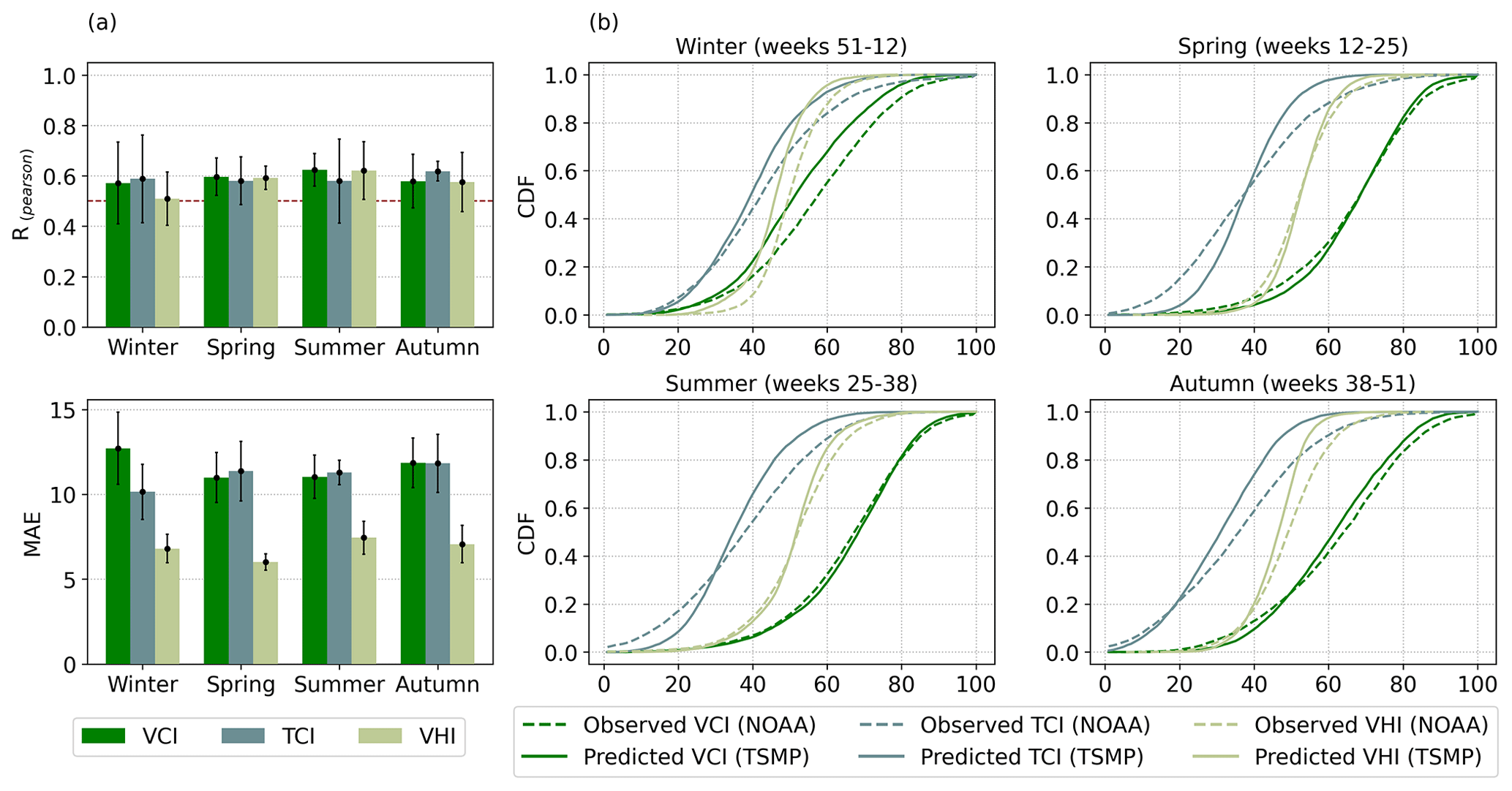
Figure 12 An evaluation of seasonally predicted agricultural drought indices with ground truth NOAA observations at a resolution of 0.88°. (a) The bottom row shows the mean absolute error (MAE) for different seasons, and the top row shows Pearson correlations (R_p) for these seasons. (b) Comparison of the cumulative distribution functions between predictions and observations.

Finally, as observed from the plots, the thermal surface condition represented by the TCI contributes more to the agricultural drought events over Europe than the deficiency in vegetation moisture condition approximated as the VCI does. This is in agreement with Zeng et al. (2023), who showed that drought affecting vegetation is more likely to be associated with abnormally high temperatures in Europe. This is critical for studies that rely on the NDVI as the sole vegetation product to identify drought events over Europe (Sect. 1). In the Appendix, we show the time series for NDVI and BT anomalies in Figs. F1 and F2. We also show vegetation health maps for different seasons from the validation and test years. These predicted maps are depicted in Fig. 10. As shown, the model predicts an increase in agricultural droughts in the summer of 2018 in central Europe and France. Xoplaki et al. (2023) associated this extremely dry summer with compound extreme events.

Furthermore, in Fig. 11, we provide an analysis of the frequency of extreme droughts for the two periods 2010–2012 and 2017–2019. Frequency represents the percent of weeks with severe to exceptional drought events where VHI < 26 (Kogan et al., 2020). While Figs. 8 and 9 provide overviews of the averaged values over the regions, the analysis in Fig. 11 provides a spatial comparison between the model prediction and observations. The major hotspots for the highest extremes are found outside the PRUDENCE regions (north of the Black Sea, northwestern Africa, Egypt, and the northwest of the Middle East). In comparison to the PRUDENCE regions, the Iberian Peninsula and France exhibit more extreme droughts. The model predicts more extreme droughts in those regions and agrees with observations. For the period 2010–2012, the model predicts fewer extreme droughts in the Mediterranean and eastern Europe, while for the 2017–2019 period the model underestimates the frequency of extremes in the central European region.

Moreover, Fig. 12 evaluates the model's capability to capture the seasonal dynamic in drought indices. As seen in Fig. 12a, the mean R_p values are greater than 0.5 and around 0.6 for all seasons. MAE values show the highest error in the VCI for the winter season. One notable observation is that the error bars have relatively large values indicating a variation in prediction accuracy across the years within the same seasons. This can be attributed to the seasonality shift in the long-term trends. Klimavičius et al. (2023) showed that meteorological forces like air temperature have a strong impact on growing seasons and phenological trends of the NDVI (VCI). The cumulative distribution functions (CDFs) in Fig. 12b express the main difference in the CDF for the VCI during winter, while the model prediction overestimates the TCI over the seasons.

4.3 Variable importance

To analyze the impact of each TSMP model component on the model prediction, we present in Table 4 the prediction results obtained with COSMO, the CLM, and ParFlow. For this experiment, we train three models based on focal modulation with the dimensionality {$C_{(\mathrm{en},\mathrm{1})}=\mathrm{64},C_{(\mathrm{en},\mathrm{2})}=\mathrm{128},C_{(\mathrm{en},\mathrm{3})}=\mathrm{256}$}. As seen in Table 4, compared to the CLM and ParFlow, COSMO achieves the best results for the validation set while the CLM outperforms both for the test set. COSMO has important variables related to water contents and clouds along with other variables related to the atmospheric effects on the reflected signal on the ground. The CLM has complementary variables related to heat fluxes and evapotranspiration. ParFlow can approximate the hydrology and serve as a proxy for the soil conditions. The results show that all model components are useful, and the best result is obtained when all these models are used.

Table 4 Impact of TSMP model components on the model performance. The metrics are shown for the validation and test sets. All models were trained with the focal modulation network. The best result of each metric is highlighted in bold text.

While Table 4 provides an overview on the importance of model components, a priori choice of proper input variables from each of these model components to predict the NDVI and BT requires substantive efforts and assumptions, especially when the underlying physical process to construct albedo and emissivity from the TSMP and trace the atmospheric effects with satellite and solar geometry is very complex. Channel attention (Woo et al., 2018; Hu et al., 2018) was commonly used in the field of computer vision and remote sensing to enhance feature representations inside DL models. A channel attention module aims to calibrate the input variables/channels by learning an input-dependent scale for each channel. Thus, it can model the inter-correlation across variables adaptively. In this work, we propose to use channel attention to determine the relative importance of TSMP input variables. Implementation details about the module are provided in Appendix B and Fig. B1. We used channel attention directly before the patch embedding for the U-Net model. To disentangle the correlation between the NDVI and the BT, we trained two separate models: one to predict the NDVI and another one to predict BT. Note that we only used channel attention for this experiment. Figure 13 provides example attentions induced for each input variable from COSMO, the CLM, and ParFlow with respect to all weeks in the test and validation sets. The attention value is the mean value, and it represents the variable importance to predict the NDVI (BT). Error bars show how the attention changes across the weeks and input samples. We observe that the distributions of attention values for the NDVI and BT are close. This indicates that the importance of highly relevant input variables is probably shared for both the NDVI and the BT. In addition, the standard deviations (error bars) suggest that the choice of prior explanatory variables is not trivial since the relative importance can change with time and input samples.

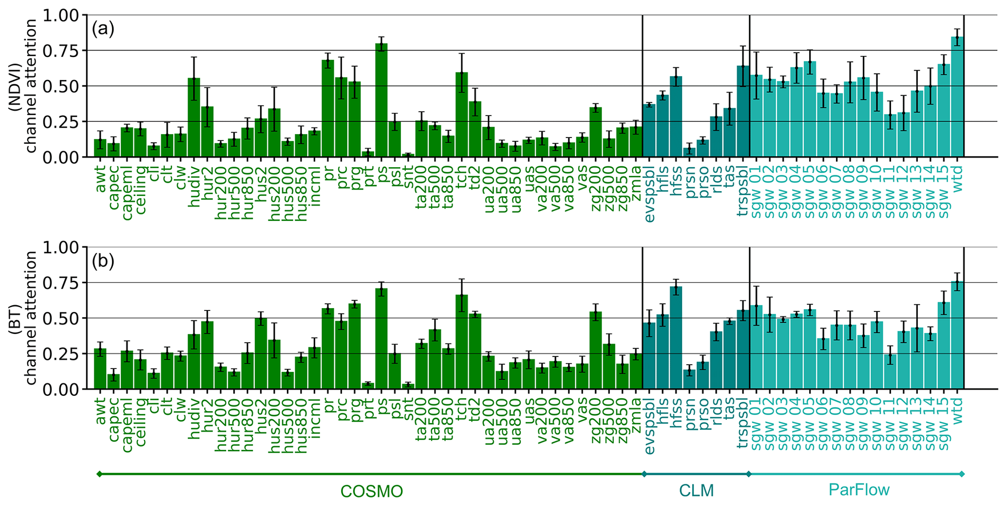
Figure 13 Channel attention for TSMP input variables. The activations are shown for both the NDVI (a) and the BT (b) with respect to all weeks in the validation and test sets.

Overall, not all variables are relevant for the model. For COSMO, atmosphere water divergence (hudiv), humidity-related variables (hus, hur), precipitation variables (pr, prc, prg), surface air pressure (ps), drag coefficient of heat (tch), and geopotential height (zg200) receive the highest attention from the DL model. For the CLM, all variables are considered important, with snowfall flux (prsn) and precipitation on ground (prso) being less important. Regarding ParFlow variables, it can be seen that the model considers most underground water-related variables as relatively important. This is intuitive since water and the amount of underground water storage are important factors for the vegetation growth. The availability of groundwater supply can reduce vulnerability to agricultural drought (Meza et al., 2020; Ma et al., 2021). Some previous studies showed that precipitation and temperature are strong predictors of the NDVI (Miao et al., 2015; Wu et al., 2020; Gao et al., 2023). In addition, the climatology of the long-term NDVI is highly correlated with precipitation and the biome classification (Yang et al., 2021b). The relatively high value for zg200 in BT prediction can be explained as the decrease in zg200 increases the likelihood of heat wave occurrence (Miralles et al., 2019). The attention values for COSMO can be interpreted as Nagol et al. (2009) showed that scattering and absorption in the atmosphere affect the visible and near-infrared radiance considerably. Shi et al. (2018) and Geiss et al. (2021) analyzed the influence of cloud-related parametrization on visible and infrared satellite images and found that the accuracy is closely related to the cloud representation. A further study about the impact of surface- and air pressure and water- and ice clouds on visible and near-infrared bands can be found in Baur et al. (2023). It needs to be emphasized that the correlations shown in Fig. 13 must not be interpreted as a causal reasoning. One main reason is that data in Earth science are subject to complicated interactions and are inherently interdependent. There may be hidden confounding variables that influence the explanatory variables and the evolution of the climate and vegetation variability. It is also worth noting that the learned variable importance by machine learning models is dependent on how the variables are represented in the training data (Betancourt et al., 2022). Furthermore, some variables have larger biases than others since the TSMP was run in a free-mode simulation. This may drive the model to rely less on such variables even if they are considered important in scientific literature. The same thing applies to highly correlated variables where changing the model architecture may alter dependencies as well (Betancourt et al., 2022).

5 Conclusions and outlook

In this paper, we presented a new deep-learning-based approach for vegetation health prediction from a regional climate simulation. The developed model enabled the prediction of variables which are not part of the input simulation. In particular, we developed a vision transformer model with focal modulation to predict NDVI and BT images from a long-term TSMP ground-to-atmosphere (G2A) simulation at 0.11° resolution and on a weekly basis. We further validated the approach with NOAA remote sensing satellite observations and identified regions of uncertainty in the model predictions. As part of this, agricultural drought assessment was performed based on vegetation health products, namely the VCI, TCI, and VHI, which were derived from the predicted NDVI and BT, and long-term climatology. In this regard, the applicability of the model was spatially and temporally analyzed on a continental scale. Additionally, we extended the commonly used explanatory variables by using plenty of TSMP variables and analyzed their relative importance for the task with channel attention as an explainable AI method. The evaluation confirms that a DL model that was trained on observations has the capacity to predict the NDVI and BT from a TSMP climate simulation with a sufficiently good agreement with real-world satellite observations.

Although our model is trained to predict vegetation products as they would be observed from the AVHRR platform, it would be possible to predict target variables from different platforms or by following different atmospheric corrections. This could be done as future work by training multiple DL models. Moreover, our work can be extended to predict other vegetation products from different satellite platforms depending on requirements. The proposed approach can be used to predict future trends in the vegetation dynamic based on climate scenarios. Providing this information, the model can help to recognize regions that are expected to be more vulnerable to agricultural drought risks. The predicted satellite-based indices can be combined with different meteorological drought indices to provide more comprehensive drought assessments under future climate change. We believe that our approach could also be useful to combine deep learning with data assimilation, i.e., to simulate remote sensing products from downscaled simulations and to be used as a supportive evaluation framework to further investigate the predictive capability of the simulation to reproduce drought events and consequently to improve the TSMP model development.

Appendix A: Datasets

Table A1 Technical details on the output variables in the TSMP EUR-11 simulation. For more information on the data, we refer to Furusho-Percot et al. (2019a).

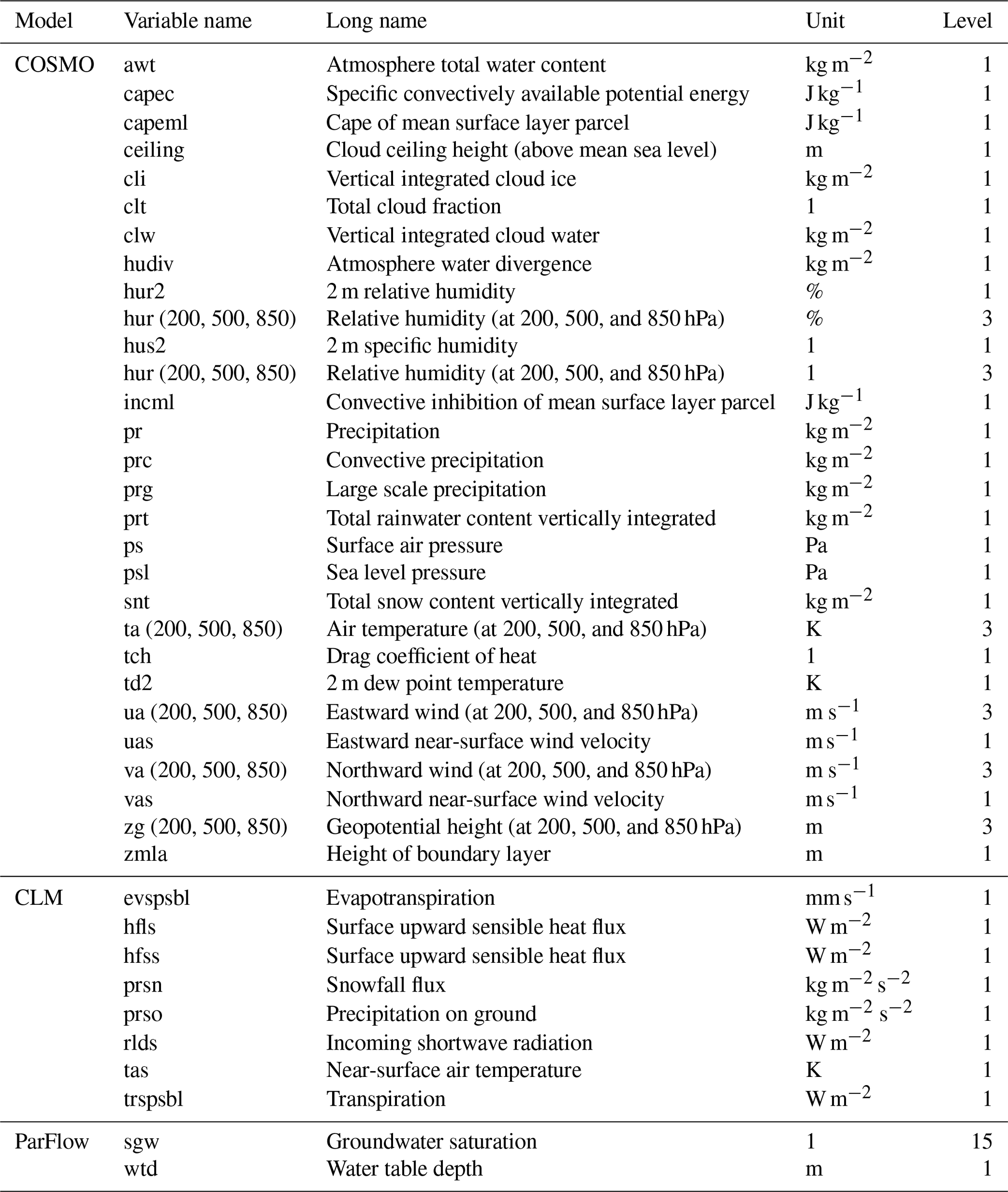
Table A2 Technical details on the static variables from the CLM in the TSMP EUR-11 simulation and the computed static variables.

Table A3 Technical details on the spectral channel characteristics for the Advanced Very-High-Resolution Radiometer (AVHRR) and the Visible Infrared Imaging Radiometer Suite (VIIRS).

Appendix B: Channel attention

Channel attention aims to condense the input channels into a lower dimensionality and then construct channel scales with a sigmoid activation function ($\text{Sigmoid}\left(x\right)=\frac{\mathrm{1}}{\mathrm{1}+{\mathrm{e}}^{-x}}\in [\mathrm{0},\mathrm{1}]$). In this manner, the neural network learns to calibrate the input channels with the learned scaling depending on the input channels. Given $\mathbf{X}\in {\mathbb{R}}^{V\times W\times H}$ as input TSMP simulation, where V is the number of output variables from COSMO, the CLM, and ParFlow and W and H are the spatial extensions, the channel attention is computed as follows:

$$\begin{array}{}\text{(B1)}& \begin{array}{rl}& \text{ChannelAttention}\left(\mathbf{X}\right)\triangleq \text{Sigmoid}\\ & \left(\text{MLP}\right(\text{GAP}\left(\mathbf{X}\right))+\text{MLP}(\text{GSD}\left(\mathbf{X}\right)\left)\right)\in {\mathbb{R}}^{V\times \mathrm{1}\times \mathrm{1}},\end{array}\end{array}$$

where Sigmoid is the sigmoid function and MLP consists of two linear layers with a ReLU activation in between. The first layer decreases the dimension to $\frac{V}{r_{\mathrm{att}}}$, and the subsequent layer maps it back to V. GAP is global average pooling, and GSD is the global standard deviation. For the experiments in Sect. 4.3, we trained two separate models for the NDVI and BT independently with (r_att=3, r_att=5) and with the dimensionality {$C_{(\mathrm{en},\mathrm{1})}=\mathrm{64},C_{(\mathrm{en},\mathrm{2})}=\mathrm{128},C_{(\mathrm{en},\mathrm{3})}=\mathrm{256}$} and averaged the results.

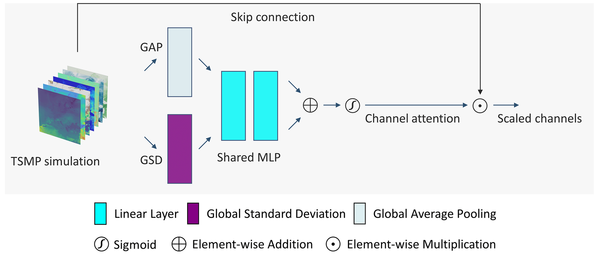
Figure B1 Illustration of the channel attention implementation. The output of channel attention is multiplied by the input TSMP to scale the channels from COSMO, the CLM, and ParFlow according to their activation values.

Appendix C: PRUDENCE scientific regions

Figure C1 Orography over the EURO-CORDEX domain. The white boundaries with the labeled names inside define the PRUDENCE regions. The time series for validating and testing agricultural drought indices were computed over these regions.

Appendix D: Ablation study

In Table D1, we provide an additional analysis of the impact of the perceptual VGG loss described in Eq. (16). When adding a perceptual loss for training, we observe a consistent improvement for all metrics while residuals are slightly bigger for the test set. As shown in Figs. D1 and D2, adding the loss ℒ_VGG reduces the blurring effect and increases variability.

Table D1 Ablation study on the perceptual VGG loss described in Eq. (16). The metrics are shown for the validation and test sets as one set. The model used is a U-Net based on focal modulation. The best result of each metric is highlighted in bold text.

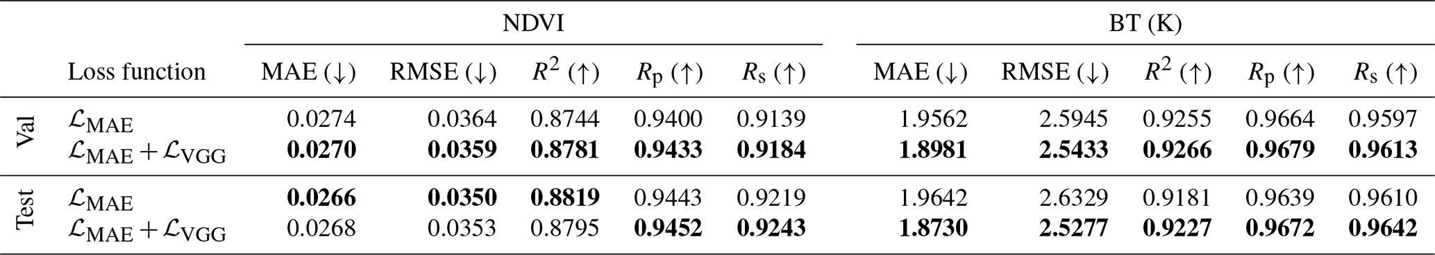
Figure D1 Impact of the perceptual VGG loss on NDVI predictions and image sharpness. The example shown is for week 30 in the year 2018. Best seen in digital formats with colors.

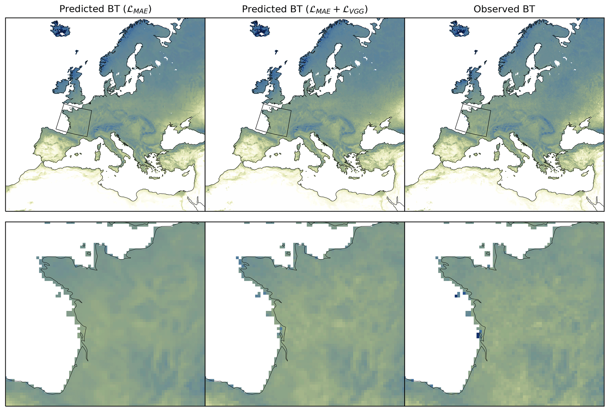
Figure D2 Impact of the perceptual VGG loss on BT predictions and image sharpness. The example shown is for week 30 in the year 2018. Best seen in digital formats with colors.

Appendix E: Patch embedding

Patch embedding with a patch size >1 is commonly used in vision transformer architectures. The main aim of this embedding is to increase the channel dimension and reduce the computational demands of the self-attention modules. This can be done by merging and embedding neighborhood pixels/tokens, thus reducing the spatial or temporal resolution. In Table E1, we show that decreasing the spatial dimension of the raw input for the encoder has negative effects on our image-to-image regression task in both quantitative and qualitative terms. This can be understood as the information was lost and the model struggles to output the original resolution. Note that for all experiments we keep using the down- and up-sampling with a factor of 2 in both the encoder and the decoder, while we only change the patch size before the first encoder layer. To match the original spatial resolution, we use an additional bilinear up-sampling after the last decoder layer.

Table E1 Impact of patch size on patch embedding before the first encoder layer. The metrics are shown for the validation and test sets. The used model is a U-Net based on the Focal Modulation model. The best result of each metric is highlighted in bold text.

Appendix F: Additional results

Figure F1 Supplementary results to Fig. 8. Comparison of spatially averaged weekly NDVI anomalies between the model prediction and NOAA observation over each PRUDENCE region. The anomaly was computed by subtracting the mean values from predictions (observations). The mean values were computed from the long-term climatology (1989-2016) pixel-wise and on a weekly basis. All results are obtained with a DL model based on the focal modulation network. The ensemble model is the result of all DL models described in Sect. 3.

Figure F2 Supplementary results to Fig. 9. Comparison of spatially averaged weekly BT anomalies between the model prediction and NOAA observation over each PRUDENCE region. The anomaly was computed by subtracting the mean values from predictions (observations). The mean values were computed from the long-term climatology (1989–2016) pixel-wise and on a weekly basis. All results are obtained with a DL model based on the focal modulation network. The ensemble model is the result of all DL models described in Sect. 3.