Implementation of additional spectral wave field exchanges in a three-dimensional wave–current coupled WAVEWATCH-III (version 6.07) and CROCO (version 1.2) configuration: assessment of their implications for macro-tidal coastal hydrodynamics

An advanced coupling between a three-dimensional ocean circulation model (CROCO) and a spectral wave model (WAVEWATCH-III) is presented to better represent the interactions of macro-tidal currents with winds and waves. In the previous implementation of the coupled interface between these two models, some of the wave-induced terms in the ocean dynamic equations were computed from their monochromatic approximations (e.g. Stokes drift, Bernoulli head, near-bottom wave orbital velocity, wave-to-ocean energy flux). In the present study, the exchanges of these fields computed from the spectral wave model are implemented and evaluated. A set of numerical experiments for a coastal configuration of the macro-tidal circulation off the Bay of Somme (France) is designed. The impact of the spectral versus monochromatic computation of wave-induced terms has a notable effect on the macro-tidal hydrodynamics, particularly in scenarios involving storm waves and opposing winds to tidal flows. This effect manifests as a reduction in the wave-induced deceleration of the vertical profile of tidal currents. The new implementation provides current magnitudes closer to measurements than those predicted using monochromatic formulations, particularly at the free surface. The spectral-surface Stokes drift and the near-bottom wave orbital velocity are found to be the spectral fields with the most impact, respectively increasing advection towards the free surface and shifting the profile close to the seabed. In the particular case of the Bay of Somme, the approximation of these spectral terms with their monochromatic counterparts ultimately results in an underestimation of ocean surface currents. Our model developments thus provide a better description of the competing effects of tides, winds, and waves on the circulation off macro-tidal bays, with implications for the study of air–sea interactions and sediment transport processes.

1 Introduction

The majority of the world's population lives in coastal environments, and the demographic predictions indicate that it will further increase in the future (Rao et al., 2008; Ioc-Unesco and FAO, 2011). The study of coastal systems therefore becomes a priority to better conciliate nature preservation and human activities, particularly in the current context of climate change. Coastal and estuarine dynamics are driven by tides and wind- and wave-induced currents and levels. The hydrodynamics in these areas induces sediment transport of fine to coarse materials, which shapes the bottom morphology and thus in turn impacts the hydrodynamics. The various components of the coastal system are thus strongly coupled and encompass scales ranging from several kilometres to less than a metre. To understand this complex dynamics, numerical modellers have worked over the last decades on coupling the different components of the coastal system.

The study of wave–current interactions is currently performed by combining wave models (spectral, monochromatic, or wave-resolved) with hydrodynamic models. To couple these models, wave forcing terms are usually added to the momentum equations, while current and water level forcing terms are added to the wave action equation when using spectral wave models. For two-dimensional horizontal (2DH) cases, equations derived by Phillips (1977) based on the pioneer works of Longuet-Higgins and Stewart (1962, 1964) using the wave radiation stress concept have been successfully implemented in numerical models to simulate wave-induced dynamics. These equations, considering the total mass transport, were adapted by Smith (2006) who separated the mass transport due to waves from that caused by the mean circulation. To improve the understanding of wave–current interactions, notably to reproduce the wave effects on the vertical profile of currents, three-dimensional modelling of the wave-induced flow was requested. Two types of theories have been developed to derive depth-dependent expressions of the wave-averaged flux of momentum due to waves and study the interaction of currents and waves in water of finite depth: the first considers the mean flow (e.g. McWilliams et al., 2004; Ardhuin et al., 2008) while the second is based on the total current (e.g. Aiki and Greatbatch, 2012, 2013; Nguyen et al., 2021). The final sets of equations obtained from these theories were successfully implemented in many hydrodynamic models for coastal (e.g. Uchiyama et al., 2010; Bennis et al., 2011; Kumar et al., 2011, 2012; Michaud et al., 2012; Moghimi et al., 2013; Bennis et al., 2014) and global applications (e.g. Couvelard et al., 2020).

In the context of the development of the Coastal and Regional Ocean COmmunity model (CROCO, https://www.croco-ocean.org, last access: 7 June 2023), the present paper contributes in investigating the sensitivity of coastal hydrodynamics to the implementation of wave-induced terms. CROCO is a new oceanic modelling system built upon ROMS-AGRIF (Shchepetkin and McWilliams, 2004; Penven et al., 2006; Debreu et al., 2012) and gradually including new features such as a non-hydrostatic kernel (Hilt et al., 2020), as well as coupling with several modules and models (atmosphere, surface waves, marine sediments, and biogeochemistry). The integration of wave–current coupling in CROCO builds upon the vortex force formalism introduced by McWilliams et al. (2004), the coupling of ROMS with the monochromatic wave model WKB embedded within the hydrodynamic framework, and the formulation of wave effects on currents in ROMS proposed by Uchiyama et al. (2009) and further advanced by Uchiyama et al. (2010). Marchesiello et al. (2015) have tested this implementation against classical test cases (e.g. planar beach, barred beach, rip currents), and they also successfully modelled the real case of the Biscarrosse beach (France), with a good representation of the rip current dynamics and the expected strong cross-shore velocities. In parallel, developments were carried out to implement a coupled interface for the air–sea exchanges including those between waves and currents by means of the OASIS-MCT coupler (Valcke et al., 2015). The interface provides a non-intrusive and flexible framework to couple with any other model that uses a similar interface. The three-way coupling (e.g. ocean–wave–atmosphere) was tested against observations (in situ and satellite) for the case of Tropical Cyclone Bejisa (2013–2014) by Pianezze et al. (2018), and a three-way coupling tutorial configuration of the Benguela region (South Africa) is also available for the user community via the CROCO documentation and tutorials (https://doi.org/10.5281/zenodo.7400922, Jullien et al., 2022).

In these former works, the exchanges of wave terms through the OASIS-MCT coupler only included significant wave height, mean or peak direction, and frequency. The wave-induced terms were then computed using a monochromatic approximation following the implementation made with the WKB model. However, in cases where the sea state is more complex than a single close-to-monochromatic wave system (e.g. multi-modal or spread spectra), the wave-induced terms computed from the full spectrum (which are provided by spectral wave models) may be significantly different from their monochromatic approximation. Various studies have shown that the monochromatic approximation for deep-water waves tends to underestimate the magnitude of the Stokes drift and the shear near the water's surface when compared to more comprehensive broadband computations (Kenyon, 1969; Rascle et al., 2006; Webb and Fox-Kemper, 2015; Lenain and Pizzo, 2020). Several alternatives for coupled models have therefore been proposed. Breivik et al. (2014) introduced a broadband approximation for the Stokes drift in deep-water conditions, and their approach has been updated to account for mixed wind-sea and swell conditions in a more recent work (Breivik and Christensen, 2020). Romero et al. (2021) presented a set of wave approximations, encompassing the Stokes drift, Bernoulli head, quasi-static pressure, and wave-induced vertical mixing. Their Stokes drift approximation builds upon the work of Breivik and Christensen (2020), employing an iterative two-scale approach capable of handling mixed wind-sea and swell conditions in finite water depths. Another approach, proposed by Kumar et al. (2017), involved spectral reconstruction from the partitioning algorithm available in WAVEWATCH-III (Hanson and Phillips, 2001).

Similar developments, which aim at adding details of the wave spectral propagation that are accounted for in the calculation of associated currents, have already been incorporated into other modelling systems, such as MOHID (Delpey et al., 2014) or SCHISM. The latter has been used to simulate and analyse wave–current interactions in various realistic scenarios, spanning both regional (Guérin et al., 2018; Lavaud et al., 2020; Pezerat et al., 2022) and coastal scales (Martins et al., 2022). Here, we evaluate the added value of using wave-induced terms computed from the WAVEWATCH-III spectral wave model instead of their monochromatic approximations computed from the WKB module in the CROCO model. We focus our study on the coastal scale of the macro-tidal environment off the Bay of Somme, in intermediate water depths and away from the nearshore breaking wave region. These developments contribute to the building of a modelling framework that enables the connection of regional, coastal, and nearshore scales, with a flexible nesting strategy and coupling. The CROCO coupled system uses the OASIS-MCT coupler, which is a set of external libraries allowing for parallel exchanges and grid interpolations between different models. This interface offers substantial flexibility, such as the possibility of coupling CROCO with any other models including a similar interface, but also the use of different grids for the various models, the adjustment of coupling frequencies, and the choice of exchanged variables, among other features.

The paper is structured as follows. In the next section the study site is introduced along with the observational data used to set up and validate the model. Section 3 is devoted to the description of the methodology. The spectral wave model is introduced along with the hydrodynamic model. The implementation of additional spectral-wave-induced terms in the hydrodynamic computation is detailed. The different coupling procedures are described, and the performed numerical experiments are summarized. Section 4 presents and discusses the numerical results. Modelled waves and currents are validated against in situ measurements. Then, the added value of the newly introduced spectral terms is evaluated considering contrasting events in terms of wind and wave forcing relative to macro-tidal currents. Section 5 is devoted to the conclusions.

2 Application site and data

The application site, Bay of Somme (hereafter named BoS), is located in the eastern part of the English Channel near Dieppe–Le Tréport (Seine-Maritime, France). BoS is the tidal inlet shown in Fig. 1.

The coastal dynamics off the bay is mainly influenced by marine (tide and waves), meteorological (wind and sea-level pressure), and fluvial (Somme's river) effects. The semi-diurnal tide is the main hydrodynamic forcing with a macro-tidal range of 8.5 m for an average spring tide and reaching 10.55 m for exceptional tides (SHOM, 2020). Tidal currents are bidirectional, oriented off the BoS to the east-northeast and west-southwest, respectively, during flood and ebb tides. Inside BoS, they flow to the east turning to southeast and to the west turning northwest for flood and ebb, respectively. Tidal asymmetry is present (SHOM, 2020), with an ebb flow (surface velocity going up to 0.95 m s⁻¹ and 2.09 m s⁻¹ off BoS and at its entrance, respectively) which is weaker than the flood (surface velocity going up to 1.2 m s⁻¹ and 2.5 m s⁻¹ off BoS and at its entrance, respectively). Ocean waves also affect hydrodynamics and are responsible for sedimentary movements offshore the bay (Ferret et al., 2010) and in the nearshore (Michel et al., 2017; Turki et al., 2021). The climatological significant wave height and period are 2 m and 7 s, respectively (Ferret et al., 2010). This indicates a not fully developed wind sea with energetic waves that develop over 400 km long fetches.

In situ data used for the validation step (wave characteristics, flow velocity magnitude and direction, and water levels) were recorded off BoS over a submarine sand dune field located in the southwest region of the study area. These data, acquired using an acoustic Doppler current profiler (ADCP) and an Aquadopp (AQDP) during a field campaign in summer 2008 (MOSAG08 survey), have been previously analysed by Ferret (2011). Only data of ADCP C3 (1 MH_z; SonTek© instruments) and AQDP B (2 MH_z; Nortek©) from 22 July to 6 August 2008 were used to validate our numerical application, because wave conditions were the most energetic at the C3 location (significant wave height reaching 2 m). The geographical positions of C3 and B mooring stations were 50°09.372^′ N, 1°17.026^′ E, and 50°08.851^′ N, 1°17.521^′ E (Fig. 1, red marks). Both profilers were immersed at a depth of 13.5 mLAT (metres below the Lowest Astronomical Tide chart datum; see Fig. 1). Measurements are the result of a 1 min average operated every 5 and 12 min, respectively, for C3 and B. These measurements were recorded at 1 m above the seabed for B and across the water column for C3 starting from 2 m above the bottom, with a 0.4 m bin resolution. At these locations, a median mass sediment diameter equal to 200 µm was observed by Ferret (2011).

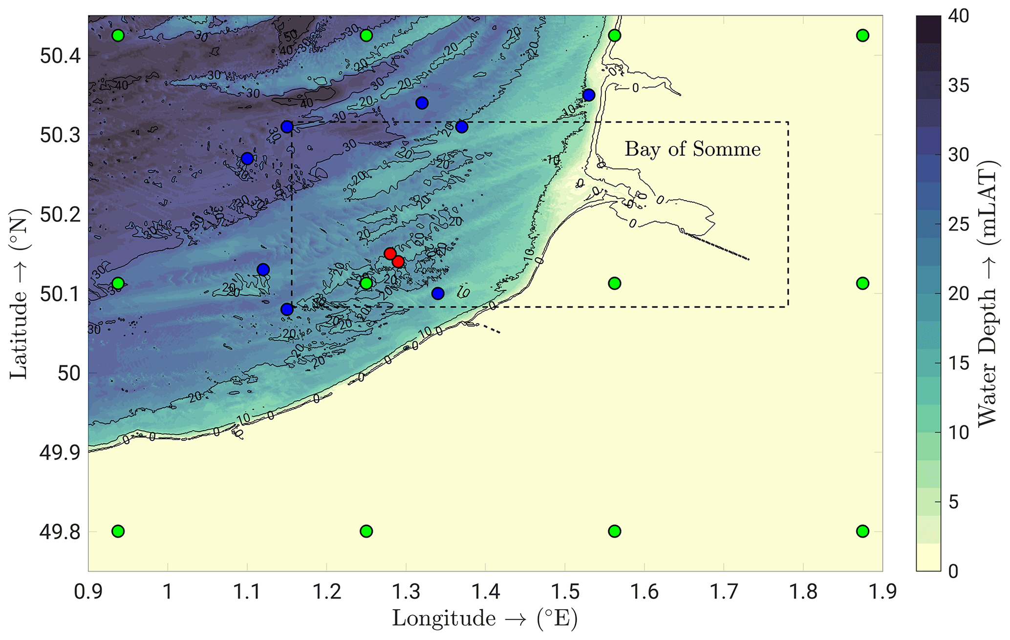
Figure 1 Bathymetric map of the study area. The dotted line encloses the computational domain. Green and blue marks indicate, respectively, the locations of the CFSR global reanalysis wind data provided by NCEP and the HOMERE wave spectral data from which wind and wave forcing are interpolated over the computational grid and its open boundaries. Red marks indicate the monitoring stations (ADCP C3 to the northwest and AQDP B to the southeast).

3 Methodology

This section presents the implemented methodology. First, the spectral wave and hydrodynamic models are introduced. Then, the new implementations for the modelling of wave–current interactions are described in detail. Lastly, the employed coupling procedures and performed numerical experiments are presented.

3.1 Spectral wave model

WAVEWATCH-III is a community wave modelling framework that includes the latest scientific advances in the field of wind-wave modelling and dynamics. The WAVEWATCH-III third-generation wave model was developed at the US National Centers for Environmental Prediction (NOAA/NCEP). In this study the version 6.07 is employed (WAVEWATCH-III®, 2019).

WAVEWATCH-III computes surface gravity wave propagation solving the discrete phase spectral action density balance equation for directional wavenumber spectra and accounts for the main physical processes influencing the propagation of waves as sinks or sources of wave energy:

$$\begin{array}{}\text{(1)}& {\displaystyle \frac{\partial }{\partial t}}N\left(\mathit{k}\right)+{\displaystyle \frac{\partial }{\partial \mathbf{x}}}\cdot \dot{\mathbf{x}}N\left(\mathit{k}\right)+{\displaystyle \frac{\partial }{\partial \mathit{\theta }}}\dot{\mathit{\theta }}N\left(\mathit{k}\right)+{\displaystyle \frac{\partial }{\partial k}}\dot{k}N\left(\mathit{k}\right)={\displaystyle \frac{S}{\mathit{\sigma }}},\text{(2)}& {\displaystyle }\dot{\mathbf{x}}=({\mathbf{c}}_{\mathrm{g}}+\mathit{u}),\text{(3)}& {\displaystyle }\dot{\mathit{\theta }}=-{\displaystyle \frac{\mathrm{1}}{k}}{\displaystyle \frac{\partial \mathit{\sigma }}{\partial h}}{\displaystyle \frac{\partial h}{\partial m}}-\mathit{k}\cdot {\displaystyle \frac{\partial \mathit{u}}{\partial m}},\text{(4)}& {\displaystyle }\dot{k}=-{\displaystyle \frac{\partial \mathit{\sigma }}{\partial h}}{\displaystyle \frac{\partial h}{\partial s}}-\mathit{k}\cdot {\displaystyle \frac{\partial \mathit{u}}{\partial s}},\end{array}$$

where $N\left(\mathit{k}\right)=F\left(\mathit{k}\right)/\mathit{\sigma }\left(k\right)$ is the wave action as a function of k, which is the wave number vector, and F(k) is the directional wavenumber spectrum; ω(k) is the frequency according to the dispersion relationship; h is the water depth; $c_{\mathrm{g}}=\partial \mathit{\sigma }/\partial \mathit{k}$ is the group velocity; u is the surface current vector; s is a coordinate in the θ direction; and m is a coordinate perpendicular to s (Tolman, 1998). The second term on the left side of Eq. (1) is the advection, the third term is the refraction, and the fourth term is direct forcing by topography and current variations. The implicit assumption of this equation is that properties of medium (water depth and current) and the wave field itself vary on temporal and spatial scales that are much larger than the variation scales of a single wave. The third-order accurate numerical scheme (Leonard, 1979) is presently used to describe wave propagation in combination with the total variance diminishing limiter (Tolman, 2002).

The source terms on the right side of Eq. (1) are integrated in time using a dynamically adjusted time-stepping algorithm, which concentrates computational efforts in conditions with rapid spectral changes. In deep waters, the dominant source terms are wave growth due to wind action S_in, nonlinear wave–wave interactions S_nl, and whitecapping S_ds. Presently, nonlinear wave–wave interactions are modelled using the discrete interaction approximation (Hasselmann et al., 1985), while input and dissipation source terms are based on Ardhuin et al. (2010). Proceeding into shallow waters, additional source terms must be included as bottom friction S_bot and depth-induced breaking S_db. In this study, the parameterization of bottom friction for sandy bottoms (Tolman, 1994) is employed as later calibrated by Ardhuin et al. (2003) in field measurements (Zhang et al., 2009). Depth-induced breaking is modelled following the formulation of Battjes and Janssen (1978).

3.2 Hydrodynamic model

CROCO (Coastal and Regional Ocean COmmunity model, https://doi.org/10.5281/zenodo.7415343, Auclair et al., 2022) is a new oceanic modelling system built upon the ROMS-AGRIF model (Shchepetkin and McWilliams, 2004; Penven et al., 2006; Debreu et al., 2012). It solves finite-difference approximations of the Reynolds-averaged Navier–Stokes (RANS) equations on a horizontal free-surface Arakawa C grid and vertical stretched terrain-following coordinates with a split-explicit time-stepping algorithm. CROCO has a flexible structure that allows choosing several numerical schemes and parameterizations. Here we use the model with the hydrostatic and Boussinesq approximations, the WENO5 scheme (Acker et al., 2016) for horizontal and vertical advection, the generic length scale scheme for vertical mixing based on the k–ϵ turbulent closure (Jones and Launder, 1972; Umlauf and Burchard, 2005; Warner et al., 2005), and the parameterization of sub-grid-scale processes in the bottom boundary layer considering the combined wave–current drag as in Soulsby and Clarke (2005). Momentum, scalar advection, and diffusive processes are represented using transport equations.

For the phase-averaged wave–current interactions, the following equations are solved in Eulerian framework and Cartesian coordinates (Uchiyama et al., 2010; Marchesiello et al., 2015) using hydrostatic, Boussinesq, and incompressible assumptions:

$$\begin{array}{}\text{(5)}& \left\{\begin{array}{lllllllll}& & & & \mathrm{\nabla }\cdot {\mathbf{v}}_{\mathrm{L}}& =& \mathrm{0},& & \\ {\displaystyle \frac{\partial u}{\partial t}}& +& \mathrm{\nabla }\cdot \left({\mathbf{v}}_{\mathrm{L}}u\right)& -& f{v}_{\mathrm{L}}& =& {\displaystyle }-{\displaystyle \frac{\partial {\mathit{\varphi }}^{\mathrm{c}}}{\partial x}}& & \\ & & & & & +& {\displaystyle }\left(u_{\mathrm{s}}{\displaystyle \frac{\partial u}{\partial x}}+v_{\mathrm{s}}{\displaystyle \frac{\partial v}{\partial x}}\right)& +& {\mathcal{F}}_u\\ & & & & & +& {\mathcal{D}}_u& +& {\mathcal{F}}_u^{\mathrm{w}},\\ {\displaystyle \frac{\partial v}{\partial t}}& +& \mathrm{\nabla }\cdot \left({\mathbf{v}}_{\mathrm{L}}v\right)& +& f{u}_{\mathrm{L}}& =& {\displaystyle }-{\displaystyle \frac{\partial {\mathit{\varphi }}^{\mathrm{c}}}{\partial y}}& & \\ & & & & & +& {\displaystyle }\left(u_{\mathrm{s}}{\displaystyle \frac{\partial u}{\partial y}}+v_{\mathrm{s}}{\displaystyle \frac{\partial v}{\partial y}}\right)& +& {\mathcal{F}}_v\\ & & & & & +& {\mathcal{D}}_v& +& {\mathcal{F}}_v^{\mathrm{w}},\\ & & {\displaystyle \frac{\partial {\mathit{\varphi }}^{\mathrm{c}}}{\partial z}}& +& {\displaystyle \frac{\mathit{\rho }g}{{\mathit{\rho }}_{\mathrm{0}}}}& =& {\displaystyle }{\mathit{v}}_{\mathrm{s}}\cdot {\displaystyle \frac{\partial \mathit{v}}{\partial z}},& & \end{array}\right.\end{array}$$

where ${\mathit{v}}_{\mathrm{L}}=(u_{\mathrm{L}},v_{\mathrm{L}},w_{\mathrm{L}})$ is the phase-averaged Lagrangian velocity, $\mathit{v}=(u,v,w)$ is the phase-averaged Eulerian velocity, and ${\mathit{v}}_{\mathrm{s}}=(u_{\mathrm{s}},v_{\mathrm{s}},w_{\mathrm{s}})$ is the 3D Stokes velocity. The phase-averaged Lagrangian velocity is calculated such that ${\mathit{v}}_{\mathrm{L}}=\mathit{v}+{\mathit{v}}_{\mathrm{s}}$. 𝒟_u and 𝒟_v are diffusive terms including wave-enhanced drag and mixing. ℱ_u and ℱ_v are forcing terms (in the present study we only consider winds at the free surface), while ${\mathcal{F}}_u^{\mathrm{w}}$ and ${\mathcal{F}}_v^{\mathrm{w}}$ are wave-induced forcing terms. ρ₀ is the reference density, g is the gravity acceleration, and f is the Coriolis parameter. ${\mathit{\varphi }}^{\mathrm{c}}=\mathit{\varphi }+\widehat{\mathit{\varphi }}$ is related to the fluid pressure, where ϕ is the dynamic pressure calculated such that ${\displaystyle }\mathit{\varphi }={\displaystyle \frac{P}{{\mathit{\rho }}_{\mathrm{0}}}}$ (with P the total pressure) and $\widehat{\mathit{\varphi }}$ is the Bernoulli head due to waves.

3.3 Wave–current interactions and new implementation of spectral-wave-induced terms

In the v1.1 of CROCO, the wave-induced terms in the ocean dynamic equations (Stokes drift, Bernoulli head, bottom wave orbital velocity, wave-to-ocean energy flux) are computed from their monochromatic approximations, which are introduced in the next subsections. In the present study, we have implemented the exchanges of these fields computed from the spectral wave model. These implementations are now included in CROCO v1.2. The formulation of the wave-induced terms in these two CROCO versions is detailed below.

3.3.1 Stokes drift

In CROCO v1.1, the Stokes velocity is calculated from the monochromatic formulation such that

$$\begin{array}{}\text{(6)}& \begin{array}{ccc}{\displaystyle }{u}_{\mathrm{s}}& =& {\displaystyle \frac{A^{\mathrm{2}}\mathit{\sigma }}{\mathrm{2}{\sinh }^{\mathrm{2}}\left(kD\right)}}\cosh \left(\mathrm{2}k\right(z+h\left)\right)k_x,\\ {\displaystyle }{v}_{\mathrm{s}}& =& {\displaystyle \frac{A^{\mathrm{2}}\mathit{\sigma }}{\mathrm{2}{\sinh }^{\mathrm{2}}\left(kD\right)}}\cosh \left(\mathrm{2}k\right(z+h\left)\right)k_y,\end{array}\end{array}$$

where A is the wave amplitude, σ is its intrinsic frequency, $\mathit{k}=(k_x,k_y)$ is the wavenumber vector, D is the mean depth, h is the bathymetric depth, and z is the vertical coordinate. Due to the non-divergence of the Stokes velocity, the vertical component is obtained from the horizontal ones:

$$\begin{array}{}\text{(7)}& {\displaystyle }{w}_{\mathrm{s}}={\displaystyle }-\underset{-h}{\overset{z}{\int }}\left({\displaystyle \frac{\partial u_{\mathrm{s}}}{\partial x}}+{\displaystyle \frac{\partial v_{\mathrm{s}}}{\partial y}}\right)\mathrm{d}{z}^{\prime }.\end{array}$$

As the Stokes drift velocity is known to be dependent on wave frequencies at the surface, we have implemented in the new CROCO v1.2 the use of the spectral formulation of the velocity at the free surface ${\mathit{v}}_{\mathrm{ss}}=(u_{\mathrm{ss}},v_{\mathrm{ss}})$ computed by WAVEWATCH-III as follows:

$$\begin{array}{}\text{(8)}& \begin{array}{rl}(u_{\mathrm{ss}},v_{\mathrm{ss}})& =\int \int \mathit{\sigma }\cosh \left(\mathrm{2}kD\right){\displaystyle \frac{\left(k\cos \right({\mathit{\theta }}_{\mathrm{w}}),k\sin ({\mathit{\theta }}_{\mathrm{w}}\left)\right)}{{\sinh }^{\mathrm{2}}\left(kD\right)}}\\ & \cdot F(k,{\mathit{\theta }}_{\mathrm{w}})\mathrm{d}k\mathrm{d}{\mathit{\theta }}_{\mathrm{w}},\end{array}\end{array}$$

where F(k,θ) is the wavenumber-direction energy spectrum (with θ_w the mean wave direction). From these surface Stokes velocity components, the dispersion relationship (σ²=gktanh (kD)), and the expansion of the hyperbolic functions describing the vertical distribution of the wave field, it is possible to obtain the following formulation for the 3D Stokes velocity field through the water column:

$$\begin{array}{}\text{(9)}& \begin{array}{rl}\left(u_{\mathrm{s}}\left(z_{\mathrm{r}}\right),v_{\mathrm{s}}\left(z_{\mathrm{r}}\right)\right)& =(u_{\mathrm{ss}},v_{\mathrm{ss}})\left[{\displaystyle \frac{\mathrm{1}}{\mathrm{2}k(\mathrm{1}+e^{-\mathrm{4}kD})}}\right]\\ & \cdot {\displaystyle \frac{\mathrm{1}}{z_{\mathrm{up}}-z_{\mathrm{low}}}}\left[\left(e^{\mathrm{2}k(z_{\mathrm{up}}+h-D)}-e^{-\mathrm{2}k(z_{\mathrm{up}}+h+D)}\right)\right.\\ & \left.-\left(e^{\mathrm{2}k(z_{\mathrm{low}}+h-D)}-e^{-\mathrm{2}k(z_{\mathrm{low}}+h+D)}\right)\right],\end{array}\end{array}$$

where z_r, z_up, and z_low represent, respectively, the vertical coordinate of the levels at RHO points (located at the centre of the computational cells) and those of the surrounding PSI points (located at the edge of the computational cells). The interested reader is referred to the CROCO manual (https://doi.org/10.5281/zenodo.7400922, Jullien et al., 2022) for a comprehensive description of the staggered computational grids and the vertical terrain-following sigma layering.

3.3.2 Bernoulli head

The wave-induced pressure called Bernoulli head ($\widehat{\mathit{\varphi }}$) is computed in CROCO v1.1 with the following monochromatic formulation:

$$\begin{array}{}\text{(10)}& \widehat{\mathit{\varphi }}={\displaystyle \frac{A^{\mathrm{2}}\mathit{\sigma }}{\mathrm{4}k{\sinh }^{\mathrm{2}}\left(kD\right)}}\underset{-h}{\overset{z}{\int }}{\displaystyle \frac{{\partial }^{\mathrm{2}}\mathit{k}\cdot \mathit{v}}{\partial z^{\prime \mathrm{2}}}}\sinh \left(\mathrm{2}k\right(z-z^{\prime }\left)\right)\mathrm{d}{z}^{\prime }.\end{array}$$

In the new v1.2, we have implemented the use of the spectral Bernoulli head computed by WAVEWATCH-III:

$$\begin{array}{}\text{(11)}& \widehat{\mathit{\varphi }}=g\int \int {\displaystyle \frac{k}{\sinh \left(\mathrm{2}kD\right)}}F(k,\mathit{\theta })\mathrm{d}k\mathrm{d}\mathit{\theta }.\end{array}$$

3.3.3 Near-bottom wave orbital velocity

Ocean waves also produce changes in bottom friction due to the enhancement of bottom drag and mixing as well as streaming effects. The parameterization of Soulsby (1997) is used for modelling bottom stresses in the presence of waves,

$$\begin{array}{}\text{(12)}& {\mathit{\tau }}_{\mathrm{wc}}={\mathit{\tau }}_{\mathrm{c}}\left(\mathrm{1}+\mathrm{1.2}{\left({\displaystyle \frac{{\mathit{\tau }}_{\mathrm{w}}}{{\mathit{\tau }}_{\mathrm{w}}+{\mathit{\tau }}_{\mathrm{c}}}}\right)}^{\mathrm{3.2}}\right),\end{array}$$

where current (τ_c) and wave (τ_w) related shear stresses are

$$\begin{array}{}\text{(13)}& {\mathit{\tau }}_{\mathrm{c}}={\displaystyle \frac{{\mathit{\kappa }}^{\mathrm{2}}}{{\ln }^{\mathrm{2}}(z/z_{\mathrm{0}})}}\mathrm{|}\mathit{u}{\mathrm{|}}^{\mathrm{2}},\end{array}$$

with z₀ the bottom roughness length and κ the von Kármán constant,

$$\begin{array}{}\text{(14)}& {\mathit{\tau }}_{\mathrm{w}}={\displaystyle \frac{\mathit{\rho }{f}_{\mathrm{w}}{u}_{\mathrm{w}}^{\mathrm{2}}}{\mathrm{2}}},\end{array}$$

with ${\displaystyle }{f}_{\mathrm{w}}={\displaystyle }\mathrm{1.39}{\left({\displaystyle \frac{u_{\mathrm{w}}}{{\mathit{\sigma }}_p{z}_{\mathrm{0}}}}\right)}^{-\mathrm{0.52}}$ the wave friction factor. u_w is the near-bottom wave orbital velocity, which is calculated in v1.1 using its monochromatic formulation:

$$\begin{array}{}\text{(15)}& u_{\mathrm{w}}={\mathit{\sigma }}_{\mathrm{p}}{\displaystyle \frac{H_{\mathrm{s}}}{\mathrm{2}\sinh \left(kD\right)}},\end{array}$$

where H_s is the significant wave height and σ_p is the peak wave frequency from the linear wave theory (Airy, 1845). In the newly implemented v1.2, the spectral near-bottom wave orbital velocity computed by WAVEWATCH-III is used instead of its monochromatic counterpart:

$$\begin{array}{}\text{(16)}& u_{\mathrm{w}}=\sqrt{\mathrm{2}}{\left(\mathrm{2}\int \int {\displaystyle \frac{{\mathit{\sigma }}^{\mathrm{2}}}{{\sinh }^{\mathrm{2}}\left(kD\right)}}F(k,\mathit{\theta })\mathrm{d}k\mathrm{d}\mathit{\theta }\right)}^{\mathrm{1}/\mathrm{2}}.\end{array}$$

3.3.4 Wave-to-ocean energy flux

In the wave-averaged momentum equations of the CROCO model, the acceleration induced by wave breaking enters as a body force:

$$\begin{array}{}\text{(17)}& {\mathcal{F}}_{u,v}^{\mathrm{w}}={\displaystyle \frac{{\mathit{ϵ}}_{\mathrm{b}}}{\mathit{\rho }\mathit{\sigma }}}{k}_{x,y}{f}_{\mathrm{b}}\left(z\right),\end{array}$$

where f_b(z) is a normalized vertical distribution function representing the vertical penetration of momentum, and ϵ_b is the depth-integrated rate of wave energy dissipation due to wave breaking. The parameterization for ϵ_b is crucial for both the wave and the circulation model to respectively compute wave dissipation and associated current acceleration. In CROCO v1.1, only few formulations of depth-induced wave breaking were implemented, and these differ from those available in WAVEWATCH-III. In this study the formulation of Battjes and Janssen (1978) is employed as it is currently available in WAVEWATCH-III, and its implementation in CROCO is straightforward. Furthermore, the spectral rate of wave-breaking dissipation computed by WAVEWATCH-III also accounts for deep-water breaking due to whitecapping such that

$$\begin{array}{}\text{(18)}& {\mathit{ϵ}}_{\mathrm{b}}=\int \int S_{\mathrm{ds}}(k,\mathit{\theta })+S_{\mathrm{db}}(k,\mathit{\theta })\mathrm{d}k\mathrm{d}\mathit{\theta },\end{array}$$

where S_ds is the deep-water dissipation term, which includes the wave energy dissipation due to whitecapping (WAVEWATCH-III®, 2019), while S_db is the shallow-water dissipation term representing the bathymetric wave breaking. The latter is computed in WAVEWATCH-III following Battjes and Janssen (1978):

$$\begin{array}{}\text{(19)}& S_{\mathrm{db}}(k,\mathit{\theta })=-\mathrm{0.25}\mathit{\alpha }{Q}_{\mathrm{b}}{f}_{\mathrm{m}}{\displaystyle \frac{H_{\max }}{E}}F(k,\mathit{\theta }),\end{array}$$

where α is a tunable parameter (α=1 in this study), H_max=γD is the maximum height a component in the random wave field can reach without breaking, γ is a constant derived from field and laboratory observations (γ=0.73 in this study), and f_m is the mean wave frequency. Q_b is the fraction of breaking waves in the random field evaluated in terms of the ratio of H_max and H_rms, which is the root-mean-square wave height such that

$$\begin{array}{}\text{(20)}& {\displaystyle \frac{\mathrm{1}-Q_{\mathrm{b}}}{-\ln \left(Q_{\mathrm{b}}\right)}}={\left({\displaystyle \frac{H_{\mathrm{rms}}}{H_{\max }}}\right)}^{\mathrm{2}}.\end{array}$$

In CROCO v1.2, we have implemented the formulation of Battjes and Janssen (1978) for ϵ_b to compute the rate of wave energy dissipation due to depth-induced breaking using mean wave parameters as well as the alternative exchange of the spectral wave energy dissipation as directly provided by WAVEWATCH-III, including deep-water breaking (whitecapping) dissipation.

3.3.5 Turbulent mixing

As anticipated in the introducing paragraph of this section, the computation of the vertical viscous and diffusion coefficients is based on the generic length scale parameterization (Umlauf and Burchard, 2005) and specifically on the k–ϵ turbulence closure scheme (Jones and Launder, 1972). Thus, the eddy viscosity of momentum and eddy diffusivity of passive tracers read

$$\begin{array}{}\text{(21)}& {\mathit{\nu }}_T=c_{\mathit{\mu }}(k_T^{\mathrm{2}}/{\mathit{ϵ}}_T),D_T=c_{\mathit{\mu }}^{\prime }(k_T^{\mathrm{2}}/{\mathit{ϵ}}_T),\end{array}$$

where c_μ and $c_{\mathit{\mu }}^{\prime }$ are coefficients determined according to the stability functions of Canuto et al. (2001), while turbulent energy k_T and energy dissipation ϵ_T are obtained from the following transport equations,

$$\begin{array}{}\text{(22)}& {\displaystyle }\begin{array}{rl}{\displaystyle \frac{\mathrm{D}{k}_T}{\mathrm{D}t}}& ={\displaystyle \frac{\partial }{\partial z}}\left({\displaystyle \frac{{\mathit{\nu }}_T}{S_{\mathrm{ck}}}}{\displaystyle \frac{\partial k_T}{\partial z}}\right)+{\mathit{\nu }}_T\left[{\left({\displaystyle \frac{\partial u}{\partial z}}\right)}^{\mathrm{2}}+{\left({\displaystyle \frac{\partial v}{\partial z}}\right)}^{\mathrm{2}}\right]\\ & -{\displaystyle \frac{g}{{\mathit{\rho }}_{\mathrm{0}}}}{\displaystyle \frac{\partial \mathit{\rho }}{\partial z}}{D}_T,\end{array}\text{(23)}& {\displaystyle }\begin{array}{rl}{\displaystyle \frac{\mathrm{D}{\mathit{ϵ}}_T}{\mathrm{D}t}}& ={\displaystyle \frac{\partial }{\partial z}}\left({\displaystyle \frac{{\mathit{\nu }}_T}{S_{\mathrm{c}\mathit{ϵ}}}}{\displaystyle \frac{\partial {\mathit{ϵ}}_T}{\partial z}}\right)+{\displaystyle \frac{{\mathit{ϵ}}_T}{k_T}}\left\{{\mathit{\beta }}_{\mathrm{1}}{\mathit{\nu }}_T\left[{\left({\displaystyle \frac{\partial u}{\partial z}}\right)}^{\mathrm{2}}\right.\right.\\ & \left.\left.+{\left({\displaystyle \frac{\partial v}{\partial z}}\right)}^{\mathrm{2}}\right]-{\mathit{\beta }}_{\mathrm{3}}{\displaystyle \frac{g}{{\mathit{\rho }}_{\mathrm{0}}}}{\displaystyle \frac{\partial \mathit{\rho }}{\partial z}}{D}_T-{\mathit{\beta }}_{\mathrm{2}}{\mathit{ϵ}}_T\right\},\end{array}\end{array}$$

and the set of coefficients identified by Warner et al. (2005) is adopted: S_ck=1, S_cϵ=1.3, β₁=1.44, β₂=1.92 , β₃=1.

Since the turbulence model does not resolve the viscous sublayer, the boundary conditions are applied in this constant stress layer where it is assumed that the turbulent energy production equals its dissipation (Wilcox, 1998) and

$$\begin{array}{}\text{(24)}& k_{\mathrm{Tb}}=(u_{\mathrm{b}}^{*}{)}^{\mathrm{2}}/(c_{\mathit{\mu }}^{\mathrm{0}}{)}^{\mathrm{2}},k_{\mathrm{Ts}}=(u_{\mathrm{s}}^{*}{)}^{\mathrm{2}}/(c_{\mathit{\mu }}^{\mathrm{0}}{)}^{\mathrm{2}},\end{array}$$

where $c_{\mathit{\mu }}^{\mathrm{0}}$ is a stability coefficient based on experimental data for unstratified channel flows with a log layer solution, u^* is the friction velocity, and subscripts “b” and “s” refer to the bottom and surface, respectively. To ensure numerical stability, boundary conditions for the turbulent energy are also applied in flux form and assuming local steady-state no-gradient conditions:

$$\begin{array}{}\text{(25)}& {\left({\displaystyle \frac{{\mathit{\nu }}_T}{S_{\mathrm{ck}}}}{\displaystyle \frac{\partial k_T}{\partial z}}\right)}_{\mathrm{b}}=\mathrm{0},{\left({\displaystyle \frac{{\mathit{\nu }}_T}{S_{\mathrm{ck}}}}{\displaystyle \frac{\partial k_T}{\partial z}}\right)}_{\mathrm{s}}=\mathrm{0}.\end{array}$$

Boundary conditions for turbulent energy dissipation follow similar reasoning and yield

$$\begin{array}{}\text{(26)}& {\mathit{ϵ}}_{\mathrm{Tb}}=(u_{\mathrm{b}}^{*}{)}^{\mathrm{3}}/\mathit{\kappa }{z}_{\mathrm{b}},{\mathit{ϵ}}_{\mathrm{Ts}}=(u_{\mathrm{s}}^{*}{)}^{\mathrm{3}}/\mathit{\kappa }{z}_{\mathrm{s}}.\end{array}$$

Flux conditions are specified also for turbulent energy dissipation to prevent numerical instabilities as follows:

$$\begin{array}{}\text{(27)}& \begin{array}{rl}{\left({\displaystyle \frac{{\mathit{\nu }}_T}{S_{\mathrm{c}\mathit{ϵ}}}}{\displaystyle \frac{\partial {\mathit{ϵ}}_T}{\partial z}}\right)}_{\mathrm{b}}& =-{\displaystyle \frac{{\mathit{\nu }}_T}{S_{\mathrm{c}\mathit{ϵ}}}}(c_{\mathrm{m}}{u}^{\mathrm{0}}{)}^{\mathrm{3}}{\displaystyle \frac{\sqrt{k_{\mathrm{Tb}}}}{z_{\mathrm{b}}^{\mathrm{2}}}},{\left({\displaystyle \frac{{\mathit{\nu }}_T}{S_{\mathrm{c}\mathit{ϵ}}}}{\displaystyle \frac{\partial {\mathit{ϵ}}_T}{\partial z}}\right)}_{\mathrm{s}}\\ & =+{\displaystyle \frac{{\mathit{\nu }}_T}{S_{\mathrm{c}\mathit{ϵ}}}}(c_{\mathrm{m}}{u}^{\mathrm{0}}{)}^{\mathrm{3}}{\displaystyle \frac{\sqrt{k_{\mathrm{Ts}}}}{z_{\mathrm{s}}^{\mathrm{2}}}}.\end{array}\end{array}$$

Wave dissipation induces additional mixing of momentum in the water column (Agrawal et al., 1992). Two main sources of wave energy decay are presently included, namely wave breaking at the free surface due to depth-induced dissipation and whitecapping as well as bottom friction due to the oscillatory wave motion in the bottom boundary layer. These two sources of wave dissipation are accounted for in the turbulence model by assuming an energy cascade in which the wave energy decay is transferred to the turbulent kinetic energy (Walstra et al., 2001). Wave energy dissipation due to bottom friction is considered to produce turbulent kinetic energy by increasing the bed shear stress in the bottom boundary layer (Eq. 12). In the case of wave breaking, an additional production of turbulent energy is also considered directly associated with the depth-integrated rate of wave energy dissipation due to wave breaking (Deigaard et al., 1986). Following Kumar et al. (2012), this additional mixing is incorporated in the k–ϵ model by introducing source terms in both the turbulent kinetic energy equation and the turbulent kinetic energy dissipation equation. Turbulence due to injection of surface flux of kinetic energy is given as surface boundary conditions (Craig and Banner, 1994; Feddersen and Trowbridge, 2005):

$$\begin{array}{}\text{(28)}& {\left({\displaystyle \frac{{\mathit{\nu }}_T}{S_{\mathrm{ck}}}}{\displaystyle \frac{\partial k_T}{\partial z}}\right)}_{\mathrm{s}}={\mathit{ϵ}}_{\mathrm{w}},\end{array}$$

where ϵ_w is the downward flux of kinetic energy due to wave breaking. The surface boundary condition for ϵ_T due to breaking waves is (Carniel et al., 2009):

$$\begin{array}{}\text{(29)}& \begin{array}{rl}{\left({\displaystyle \frac{{\mathit{\nu }}_T}{S_{\mathrm{c}\mathit{ϵ}}}}{\displaystyle \frac{\partial {\mathit{ϵ}}_T}{\partial z}}\right)}_{\mathrm{s}}& =-{\displaystyle \frac{S_{\mathrm{ck}}}{S_{c\mathit{ϵ}}}}(c_{\mathit{\mu }}^{\mathrm{0}}{)}^{\mathrm{3}}{\displaystyle \frac{\mathrm{3}}{\mathrm{2}}}\sqrt{k_T}{\displaystyle \frac{\mathcal{Y}}{\mathit{\kappa }(z_{\mathrm{0}}-z_{\mathrm{s}})}}\\ & +{\displaystyle \frac{{\mathit{\nu }}_T}{S_{\mathrm{c}\mathit{ϵ}}}}(c_{\mathit{\mu }}^{\mathrm{0}}{)}^{\mathrm{3}}\sqrt{k_T}{k}_T{\displaystyle \frac{(z_{\mathrm{0}}-z_{\mathrm{s}})}{\mathit{\kappa }}},\end{array}\end{array}$$

where 𝒴 is the surface mixing length. In the case of breaking waves, the surface mixing length is provided using the closure model of Stacey (1999):

$$\begin{array}{}\text{(30)}& \mathcal{Y}={\mathit{ϵ}}_{\mathrm{w}}{z}_{\mathrm{0}},\end{array}$$

with z₀=α_wH_rms and α_w=0.5. Only part of the wave energy dissipation (ϵ_b) contributes to turbulence mixing. The contribution of wave energy dissipation as surface flux of kinetic energy is expressed through an empirical coefficient c_ϵw. Thus, the downward flux of kinetic energy due to wave breaking is

$$\begin{array}{}\text{(31)}& {\mathit{ϵ}}_{\mathrm{w}}=c_{\mathit{ϵ}\mathrm{w}}{\mathit{ϵ}}_{\mathrm{b}},\end{array}$$

According to Jones and Monismith (2008), we assume that only 5 % of wave energy dissipation goes into the water column as turbulent kinetic energy.

Figure 2 Schematic representation of the coupling between CROCO and WAVEWATCH-III using OASIS. Available coupling procedures in CROCO v1.1 are summarized on the left. Only three mean spectral wave fields (blue labels) are provided by WAVEWATCH-III in the one-way coupling (1WC), i.e. mean wave period (T_m01), significant wave height (H_S), and mean wave direction (θ_w), while in the two-way coupling (2WC) CROCO provides circulation fields (green labels), i.e. water levels (SSH) and surface currents (UZ, VZ). The newly developed coupling procedures in CROCO v1.2 are summarized on the right. In both one-way (1WF) and two-way (2WF) coupling, additional wave spectral fields (red labels) are exchanged, i.e. the mean wavelength (LM), Bernoulli head pressure (BHD), wave-to-ocean energy flux (FOC), magnitude and direction of the surface Stokes drift (USS), and near-bottom wave orbital velocity (UBR).

3.4 Coupling procedure

In this study, CROCO and WAVEWATCH-III are coupled as presented in Fig. 2. Instantaneous hydrodynamic fields are exchanged between both models every coupling time step (Δt_c=60 s) thanks to the OASIS coupler (Valcke et al., 2015), according to a similar procedure to that in Pianezze et al. (2018), Bennis et al. (2020), and Bennis et al. (2022). The choice of exchanged variables, coupling frequency, and grid interpolation options is managed through a text file read by OASIS (named namcouple). CROCO provides the sea surface height and surface flow velocity to WAVEWATCH-III, which are used in the wave model to compute depth- and current-induced wave refraction. In CROCO v1.1, WAVEWATCH-III provides only three mean wave parameters based on the integration of the wave spectrum (Fig. 2 left panel, blue labels): the significant wave height (H_s), the mean wave period (T_m01), and the mean wave direction (θ_w), which are used by CROCO to compute wave-induced terms in the hydrodynamic equations, including horizontal and vertical vortex force, wave-induced pressure, wave-induced tracer diffusivity, non-conservative wave dissipation, non-conservative wave accelerations for currents, and wave-enhanced vertical mixing (Eq. 5). In the new v1.2, we have implemented the additional exchanges of the mean wavelength (LM), near-bottom wave orbital velocity (UBR), magnitude and direction of the surface Stokes drift (USS), Bernoulli head pressure (BHD), and wave-to-ocean energy flux (FOC) from WAVEWATCH-III to CROCO (Fig. 2 right panel, red labels). These wave-induced terms are already computed from the full spectrum in the wave model. They are here exchanged through the coupler and used in CROCO wave-averaged equations instead of their monochromatic approximations, allowing a wider range of applications. The additional exchanges are coded in the cpl_prism_get.F routine of CROCO, which manages all the possibly received variables from OASIS-MCT. The use of these spectrally computed terms in the wave-averaged equations of CROCO instead of their monochromatic approximation is activated with a CPP preprocessing key (as other options in CROCO) named OW_COUPLING_FULL that can be defined in the cppdefs.h file and which impacts the choice of terms used in the mrl_wci.F (wave-averaged equations) and bbl.F (bottom boundary layer) routines. These modifications have been available in CROCO since the v1.2 release (https://doi.org/10.5281/zenodo.7415343, Auclair et al., 2022). Both the monochromatic and full coupling procedures remain accessible for comparison in different configurations, and users can easily switch between them by activating or deactivating the OW_COUPLING_FULL preprocessing key.

3.5 Numerical experiments

Each numerical experiment performed in this study considers a rectangular computational domain delimited by the points 50.316° N, 1.156° E, and 50.083° N, 1.781° E, respectively, at the NW and SE corners (Fig. 1). The same computational grid is adopted for both the wave and the circulation models, but the use of different grids is possible. The horizontal mesh has a spatial resolution of 100 m, and the bathymetry from HOMONIM (Shom, 2015) is interpolated over this grid. A total of 20 sigma layers are used for the vertical discretization. They are uniformly distributed between the seabed and the free surface, resulting in a maximum layer thickness offshore of about 2 m and a minimum layer thickness onshore of about 5 cm.

The wave model uses 32 frequencies (0.04–0.7 s⁻¹) and 24 directions, leading to a directional resolution of 15°. Bi-dimensional (frequency and direction) full wave spectra from the HOMERE database (Boudiere et al., 2013) are used to interpolate wave forcing at the deep-water open boundaries. It is worth noting that the use of full spectra at the boundaries is the recommended practice in modelling spectral waves, particularly when investigating wave–current interactions, as suggested by Kumar et al. (2017) and Liu et al. (2021).

Along these open boundaries, tidal forcing is interpolated from the high-resolution (250 m) PREVIMER atlas MANE focused on the east part of the English Channel, which includes 37 harmonic constituents (Pineau-Guillou et al., 2014). A cold start is imposed as an initial condition, and no stratification due to temperature and salinity gradients is considered. To assess the independence of the hydrodynamic results used to validate the model from the relative distance between the forcing boundaries and the measurement sites, we conducted an additional numerical simulation with an extended computational grid, effectively placing the measurement location further from the open boundaries. The results of this supplementary simulation align closely with the outputs of the simulation which solely employed tidal forcing. This congruence has been assessed in terms of circulation patterns, time series of near-bottom currents, and vertical profiles.

Wind forcing is provided by NCEP throughout hourly wind speeds at 10 m above mean sea level from the CFSR reanalysis at 0.312° horizontal resolution (Saha et al., 2010). This resolution is much coarser than the numerical model resolution, and this may have an impact on the simulation results. It is important to acknowledge this limitation and consider it when interpreting the results. Wind stresses at the free surface are computed according to the formulation of Smith (1988), which estimates the wind drag for sea surface wind stress as a function of wind speed while accounting for a constant Charnock coefficient. This approach parameterizes the impact of the sea state on the drag through the wind speed only and does not consider an eventual variation of the drag coefficient for various sea states for a given wind speed. Since the effect of waves on the wind drag have been proven to have substantial effect on free-surface currents in similar macro-tidal settings (Calvino et al., 2023), we performed a sensitivity experiment in which the surface wind stress was computed by WAVEWATCH-III (two terms) and input into CROCO, therefore accounting for the impact of varying sea states on the wind drag coefficient. This sensitivity analysis showed that while wave effects may alter wind stresses at the free surface, their impact on vertical velocity profiles is negligible under the investigated metocean conditions. This finding reinforces the robustness of the present modelling approach in forcing conditions similar to those presently investigated. Furthermore, no water and heat fluxes from the atmosphere are considered.

Hydrodynamic motions were not computed for depths smaller than 1 m while wave-induced forcing terms were activated for depths greater than 2 m. This is necessary due to the low resolution of the employed bathymetry, whose interpolation resulted in steep seabed gradients within the bay, leading to numerical instabilities in shallow waters. The observed mass median diameter of sediment particles equal to 200 µm (Ferret, 2011) is used to compute the effective Nikuradse roughness length employed in the parameterizations of bottom friction (CROCO using Soulsby, 1997, and WAVEWATCH-III using Ardhuin et al., 2010, ST4 package).

To understand the impact on the macro-tidal hydrodynamics of BoS of each metocean forcing (tide, wind, and waves) and each additional spectral field exchanged compared to its monochromatic approximation, a total of nine final numerical experiments have been performed. These simulations are detailed in Table 1. A simulation forced by only tidal levels and currents (CRX) was initially performed to be used as baseline case, providing a pure tidal vertical current profile. To assess the impact on the vertical profile of wind forcing alone, a second simulation with tidal and wind forcing (WND) was performed but without accounting for waves. Waves are then considered in all subsequent simulations. The first simulation uses the CROCO v1.1 configuration with computation of wave-induced terms from their monochromatic approximation. The five following simulations each include a different additional spectral wave field exchange instead of its monochromatic approximation (mean wavelength LM, Bernoulli head pressure BHD, wave-to-ocean energy flux FOC, surface Stokes drift USS, and near-bottom wave orbital velocity UBR). The last simulation, named full coupling, uses all the spectral-wave-induced terms included in CROCO v1.2.

Table 1 Summary of the fields exchanged within the OASIS coupler between CROCO and WAVEWATCH-III in each numerical simulation.

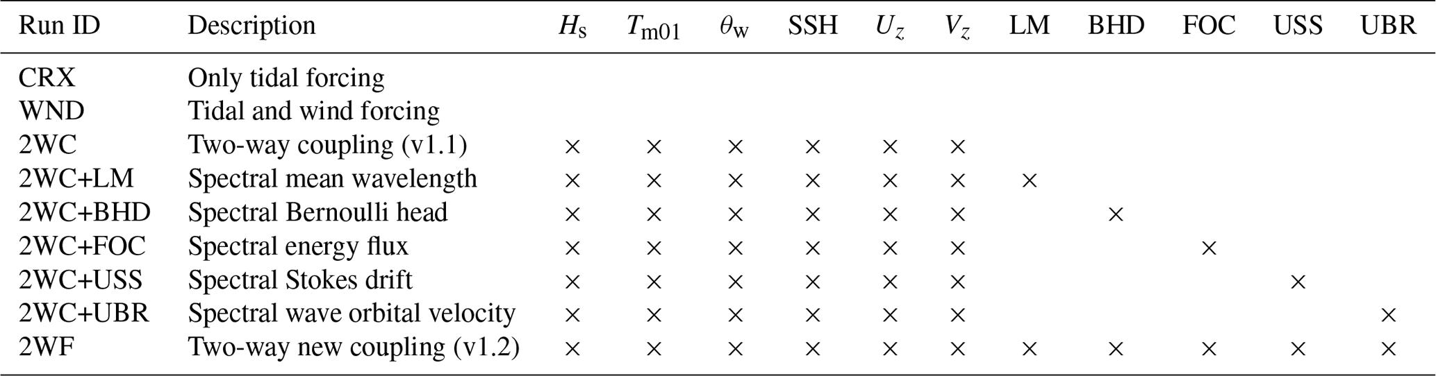
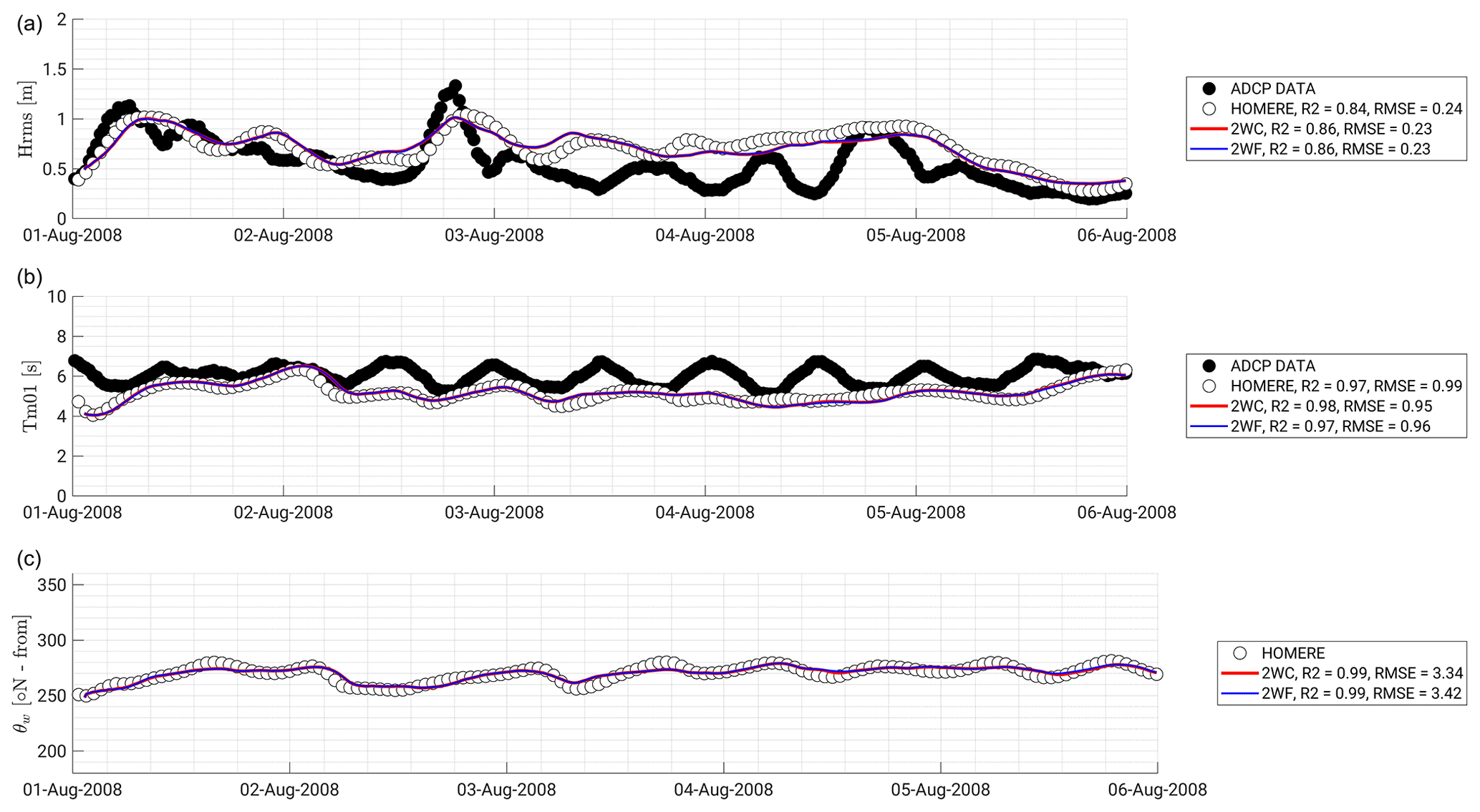
Figure 3 Time series of computed mean wave parameters. Comparisons of model results (solid lines) with in situ measurements (ADCP data, black dots) and output of the large-scale spectral wave model (HOMERE data, white dots) in terms of significant wave height (a), mean wave period (b), and mean wave direction (c). Note that statistical metrics in the bottom-left insert correspond to the correlation between modelled directions and those predicted by the HOMERE hindcast (no information was available from the ADCP).

4 Results and discussions

To assess the performance of the CROCO–WAVEWATCH-III coupled model, we compared numerical results in terms of mean wave parameters, water level, and current with in situ ADCP and AQDP measurements (red dots in Fig. 1) and with the HOMERE hindcast (Boudiere et al., 2013). Then, the impacts of the additional spectral terms on current and water level are analysed in time and space for different met-ocean conditions.

4.1 Assessment of modelled waves

Sea states were simulated for a time period ranging from 1 to 6 August 2008 (Fig. 3). During this period, an energetic wind event (fresh to strong breeze based on Beaufort's wind scale with moderate to large waves) occurred on 2 August with a wind velocity magnitude at 10 m above the sea surface reaching 10.5 m s⁻¹ between 17:00 and 19:00 GMT+2 The root-mean-square significant wave height (H_rms) computed by WAVEWATCH-III turns out to be smaller than the observed one (top panel of Fig. 3), with a maximum value around 1.05 m instead of the observed 1.40 m, leading to an underestimation of about 25 % by the model. By contrast, simulated wave heights, periods, and directions are close to those predicted by the HOMERE hindcast (Fig. 3). For the entire time series, the correlation coefficient r² is 0.86, while RMSE is 0.23 m. This partly validates our numerical configuration. Since the HOMERE hindcast is alike in wind forcing, physical parameterizations, and computational grid size, it is consistent to obtain similar results. Moreover, this hindcast was used to force the spectral wave model at these boundaries. Slight differences between the two model predictions are thus supposedly due to the higher spatial resolution employed in the present study (100 m), which results in a better description of wave shoaling and refraction.

Figure 4 Surface current magnitudes (coloured shading) with superimposed current vectors (black arrows) computed from simulation 2WF and bathymetric contours (grey contours) at the peak of the ebb tidal flow on 2 August 2008 at 17:00 (a) and that of the flood 6 h later (b). Black circles are the ADCP and AQDP locations.

Waves are deviated from their direction of propagation by the surface currents (e.g. Ardhuin et al., 2012; Bennis et al., 2020). In the study area, the flood flow is oriented towards the east-northeast while the ebb flow goes to the west-southwest (Fig. 4). Due to the tide asymmetry often observed in the English Channel, the ebb current is less intense than the flood current with a mean value of 0.45 and 0.6 m s⁻¹, respectively, during spring tide (Ferret, 2011). Although the current magnitude is relatively weak, a change in the wave direction is observed with a slight modulation following the tidal phase, as shown in Fig. 3 (bottom panel) at the ADCP location, and this matches very well (r²=0.99) with the predictions of the HOMERE hindcast.

4.2 Assessment of modelled levels and currents

The circulation within and off the bay is mainly controlled by semi-diurnal tidal currents which are oriented to the west-southwest during ebbs (Fig. 4, top panel) and east-northeast during floods (Fig. 4, bottom panel). The model well reproduces the observed tidal asymmetry (SHOM, 2020) predicting modelled peak surface velocity magnitudes larger than 2 m s⁻¹ during flood and smaller than 1.5 m s⁻¹ during ebb in the simulated period.

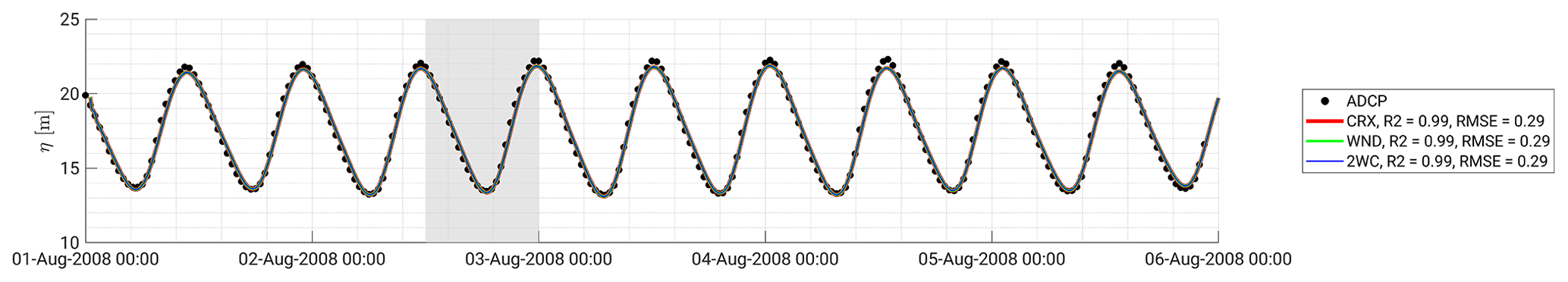
Figure 5 Comparison of modelled water levels (solid lines) with in situ measurements (dots) at the ADCP location. The shaded area shows the period of fresh to strong winds with moderate to large waves in the investigated time window.

Figure 5 shows the comparisons of our results with the ADCP data in terms of sea surface height. The hydrodynamic model well captures the macro-tidal range off the BoS (about 8 m for the simulated time period), and excellent scores are obtained (r²=0.99 and RMSE = 0.29) for all runs. Similar results are obtained with the standalone CROCO model forced only with tides (CRX), the simulation including wind forcing (WND), and the simulation accounting for waves and their interactions with levels and currents (2WC), showing that winds and waves do not significantly affect water levels at the ADCP mooring station, which are mainly controlled by tides.

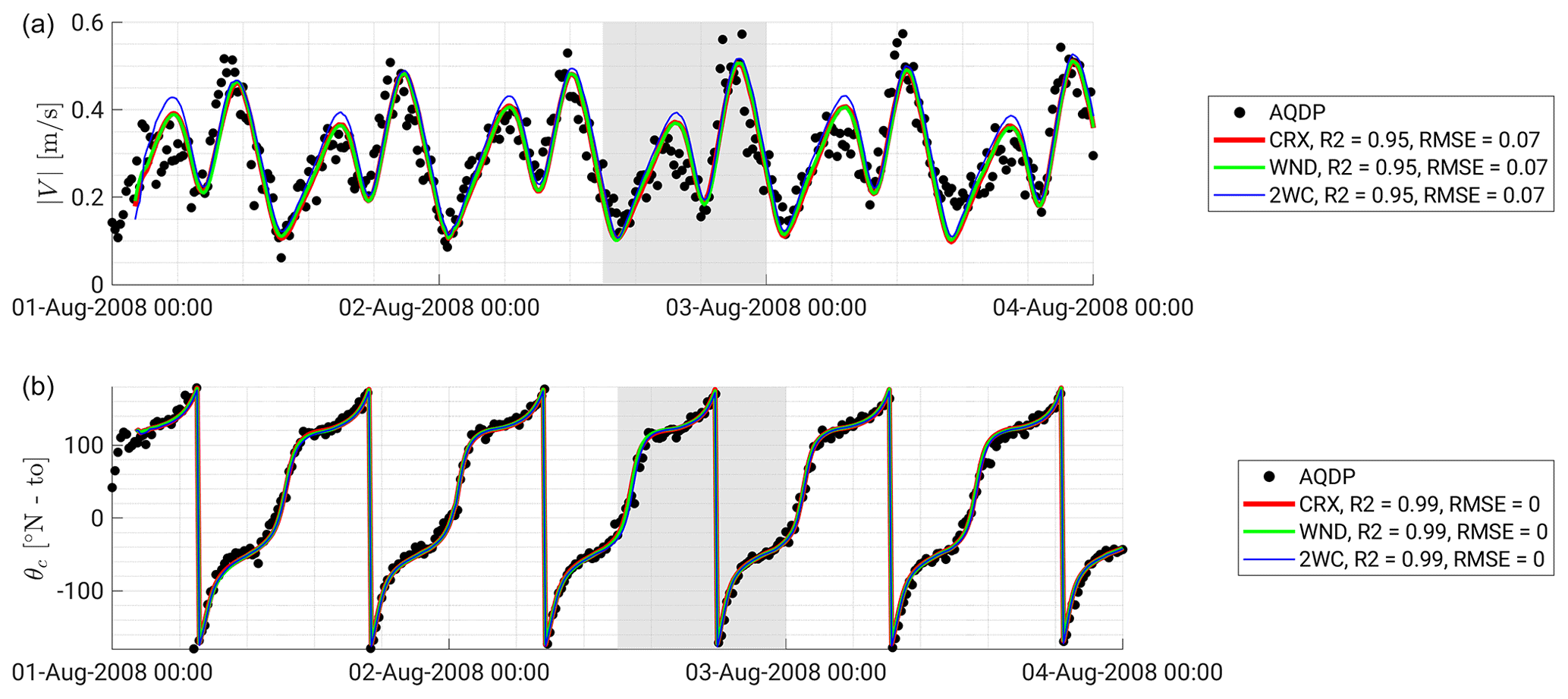
Figure 6 Time series of computed near-bottom tidal currents. Model results (lines) are compared with AQDP (dots) measurements in terms of (a) current magnitude and (b) “going to” direction at 1 m above bottom (m a.b.). Shaded areas show the period of fresh to strong winds with moderate to large waves in the investigated time window.

Figure 6 shows the comparisons of our model results with the AQDP measurements in terms of current magnitude and direction at 1 m above the bottom (m a.b.). The modelled current magnitude is correctly predicted in line with the values recorded by the AQDP during the different phases of the tidal cycle. Particularly well captured is the tidal current reversal. This is confirmed by near-bottom current directions that are shown to be fairly replicated. A small phase shift (around 10 min) between measured and modelled currents is present. This can be seen by comparing the time at which the velocity peak occurs during tidal floods. Flood peaks are reached slightly later in the model than observed in the measurements, as if the model would predict longer flood phases than observed. This phase shift could be due to bottom friction effects associated with the presence of widespread bedforms of very different sizes (e.g. Charru et al., 2013), ranging from small-scale ripples to large-scale sand waves, whose impact on hydrodynamics cannot be properly modelled using the horizontal resolution employed in the present study. Indeed, current measurements have been collected in a field of sand dunes with an average crest distance of about 425 m, which cannot be properly represented with the 100 m grid resolution. Winds and waves are shown to not significantly affect near-bottom currents which are clearly dominated by tides. Similar results have indeed been obtained with the standalone CROCO model forced only with tides (CRX), considering also the wind forcing (WND), and accounting for wave–current-level interactions (2WC).

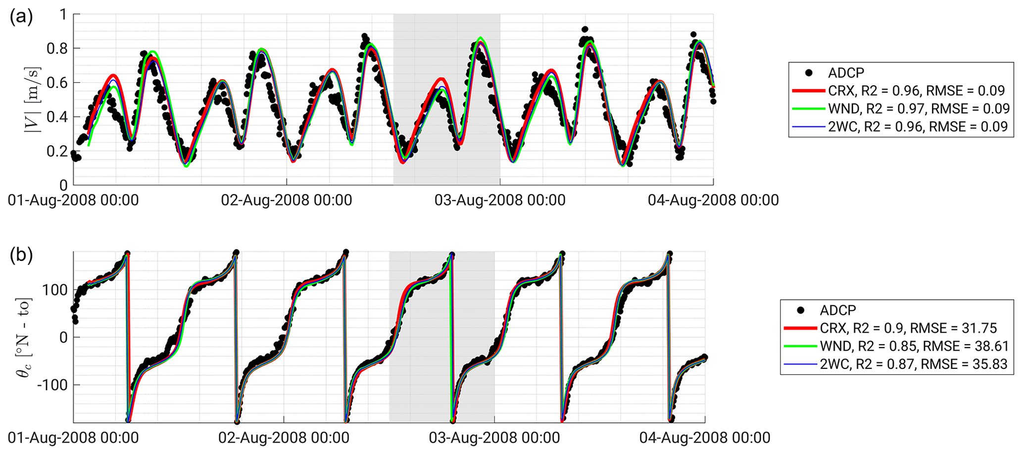
Figure 7 Same legend as for Fig. 6 but referring to the tidal currents at 1 m below the free surface (m b.f.s.).

Figure 7 shows the comparisons of model predictions with the ADCP measurements in terms of current magnitude and direction at 1 m below the free surface (1 m b.f.s.). The modelled current magnitude is correctly predicted during most of the phases of the tidal cycle, particularly at tidal current reversal and especially during ebb phases. Also, current directions are fairly replicated. The phase shift between measured and modelled currents is present also at the free surface when comparing modelled currents with the ADCP measurements. It is worth noting that peak flood velocities delay is not coincident with passing storms, thus suggesting that winds and waves are not responsible for the phase shift and adding up to the likelihood that this is due to the presence of sub-grid-scale bedforms. Results obtained by the standalone CROCO model forced only with tides (CRX) are modified by wind stresses (WND), resulting in an acceleration and a deceleration of surface currents, respectively, at tidal floods and ebbs due to winds blowing towards the east-northeast. This wind-driven modulation is pronounced during storms. Wave effects on currents tend to smooth this modulation (2WC) by means of wave–current interaction mechanisms, as explained in the following section.

Tests of model results (2WC) against in situ measurements through the water column in terms of eastward (Fig. 8) and northward (Fig. 9) current velocity components at the ADCP location further validate our modelling. Overall, the fair matching between measured and modelled current velocity components during the different phases of the tidal cycle and within the entire water column proves the reliability of the hydrodynamic model. However, an overestimation (underestimation) of the northward tidal current velocity computed by the model is observed during ebb (flood) peaks, particularly around the low tide slack water event, from the surface to the bottom.

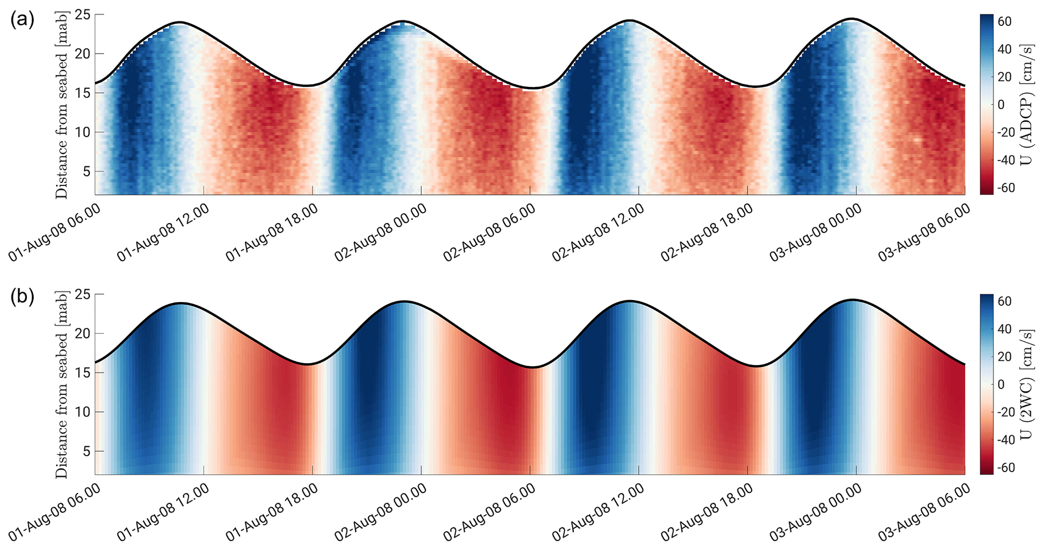
Figure 8 Time series of the measured (a) and modelled (b, 2WC) eastward tidal current velocity over the depth and at the ADCP location. Thick black line represents the free-surface elevation from the seabed in time.

Figure 9 Same legend as for Fig. 8 but for the northward tidal current velocity.

4.3 Assessment of vertical current profiles for contrasting events

To assess the importance of exchanging spectral wave fields instead of computing them from monochromatic approximations, we compared measured vertical profiles of currents extracted at noteworthy time instants within various simulations listed in Table 1. Figure 10 shows two vertical current profiles associated with storm waves and calm sea states. Measured (squares) and modelled (continuous lines) time series of current velocities (red) and root-mean-square wave heights (blue) are compared in the top panel (a). The middle panel (b) analogously compares current and wave directions. Vertical profiles were extracted at two time instants characterized by the occurrence of waves coming from west with H_rms, respectively, larger and smaller than 1 m. In the case of storm waves (bottom-left panel c), wind-driven stresses are shown to modify the logarithmic tidal velocity profile accelerating the current towards the free surface and decelerating it towards the bottom, as reported in former studies (e.g. Davies and Lawrence, 1995). However, this velocity increase seems too strong in view of the data with an overestimate of about 5 cm s⁻¹ at the surface, which represents about 18.5 % of the measured surface velocity. Wave–current coupling considering terms computed with their monochromatic approximations (CROCO v1.1, 2WC) produced a realistic surface flow which now fits the measurements very well. The smoothing of the wind-induced profile is due to waves because of the wave–current interaction mechanism described in Groeneweg and Klopman (1998), which is activated by waves moving in a direction similar to that of the current and thus opposite to the wind stress (Fig. 10c). The adding of the full wave spectral terms (CROCO v1.2) results in a light smoothing of the vertical profile throughout the entire water column, but the overall impact on model predictions is minor (Fig. 10, 2WF). In the case of calm sea states (bottom-right panel d), wind and wave effects are negligible and do not significantly modify the logarithmic tidal velocity profile.

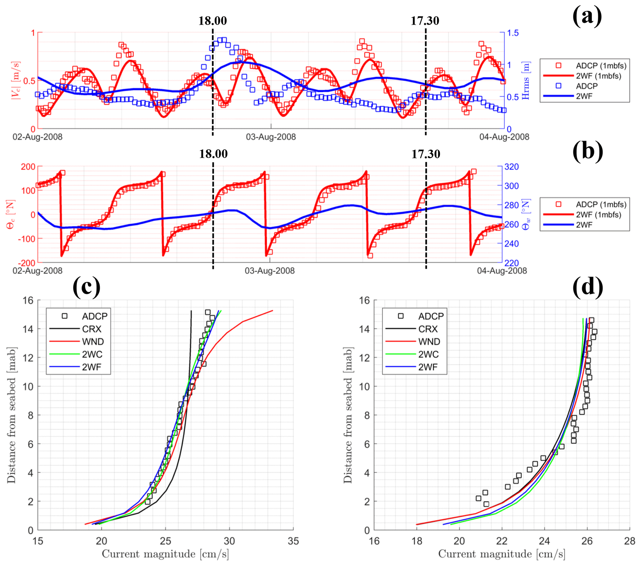
Figure 10 (a) Time series of measured (squares) and modelled (continuous lines) surface current magnitude (red) and wave heights (blue) at the ADCP location. (b) Time series of measured (squares) and modelled (continuous lines) surface current (red) and wave (blue) directions at the ADCP location. The dotted black lines indicate the two time instants at which vertical velocity profiles (c, d) are extracted for H_rms larger (c) and lower (d) than 1 m, respectively. (c) Measured (squares) and modelled (continuous lines) vertical profiles of the current on 2 August 2008 at 18:00. (d) Same legend as for panel (c) but referring to 3 August 2008 at 17:30.

Figure 11 shows two vertical current profiles associated with ∼10 m s⁻¹ winds. Measured (squares) and modelled (continuous lines) time series of current velocities (red) and wind speeds (blue) are compared in the top panel (a). The middle panel (b) analogously compares current and wind directions. Note that modelled wind speeds and directions from the CFSR global reanalysis data set are tested against the records of a Met Office mooring station in the English Channel just offshore the study area (50.4° N, 0.0° E) from the Copernicus Marine In-Situ Near Real Time Observations of the Atlantic Iberian Biscay Irish Ocean (Copernicus Marine Service, 2021). Vertical profiles were extracted at two time instants characterized by the occurrence of winds coming from west, contrasting ebb flows, and favouring flood flows. In the case of winds blowing in a direction which is opposite to that of tidal currents (bottom-left panel c), wind-driven stresses are shown to modify the logarithmic tidal velocity profile (black curve) by slowing the flow over a depth of 10 m due to wind resistance of the flow, which results in a reduction of the surface velocity magnitude of about 8 cm s⁻¹ (or 25 % of the pure tidal velocity). CROCO v1.2 coupling results in a current profile in between the logarithmic tidal profile and that of CROCO v1.1. It is closer to that of the simulation only influenced by wind stresses with a lower decrease in the close-to-surface velocity and a slight increase in the close-to-bottom velocity. The profile modelled with CROCO v1.2, while still showing significant biases with observations, is, however, the best fitting with measurements throughout the entire water column compared to other simulations (Fig. 11, 2WF). Waves accelerate the wind-induced current of about 3 cm s⁻¹ at the surface due to an angle between wave and current directions of propagation slightly larger than 90°. Indeed, the wave energy spectrum at this time shows a sea state with two peak frequencies (around 0.15 and 0.25 Hz), and thus the use of spectral forcing terms improves the accuracy of the results (Fig. 11; RMSE ∼1.8 cm s⁻¹, r²=0.99). Differences between CROCO v1.1 and v1.2 are mainly related to the near-bed wave orbital velocity, which is increased by a factor of about 1.5 at this time (Fig. 12), leading to a reduction in the bottom stress (Eq. 9) due to the weak value of the near-bottom flow velocity (about 20 cm s⁻¹). This reduces the flow intensity across the entire water column, as described by Bennis et al. (2020, 2022). In the case of winds blowing in the same direction of tidal currents (bottom-right panel d), winds and waves only slightly affect the tidal logarithmic profile, leading to less significant differences. Indeed, the wind forcing magnitude at 14:30 and at 23:00 is similar, but its impact on current is minor at 23:00 as the instantaneous surface velocity magnitude is more than twice as high as at 14:30 (60 cm s⁻¹ versus 25 cm s⁻¹). As in the previous case (Fig. 10), wind stresses accelerate the tidal profile at the free surface since wind is following the current, while waves tend to smooth it.

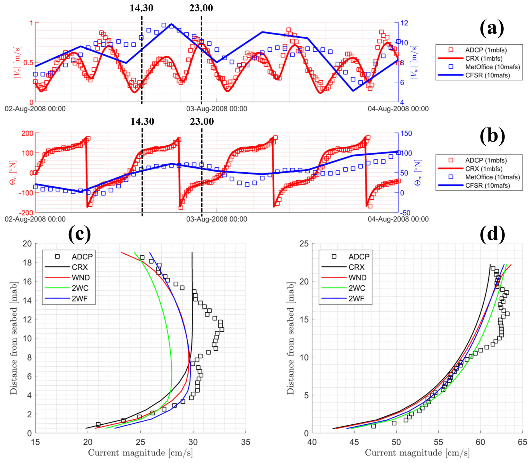
Figure 11 (a) Time series of measured (squares) and modelled (continuous lines) surface current magnitude (red) and wind speeds (blue). (b) Time series of measured (squares) and modelled (continuous lines) surface current (red) and wind (blue) directions. The dotted black lines indicate the two time instants at which vertical velocity profiles (bottom panels) are extracted, which correspond to winds coming from the southwest with speeds higher than 10 m s⁻¹ during tidal ebb (c) and flood (d). (c) Measured (squares) and modelled (continuous lines) vertical profiles of the current on 2 August 2008 at 14:30 (tide reversal). (d) Same legend as for panel (c) but referring to 2 August 2008 at 23:00 (tidal ebb).

The velocity magnitude on the water column is reduced by the use of wave spectral forcing terms because of the increase in the near-bed orbital velocity (about 2 cm s⁻¹) that causes an enhancement of the bottom stress. It is also worth noting that, in both situations, maximum current magnitude in the middle of the water column is not captured by the model. Better fits are obtained near the surface than in the middle of the water column. At 14:30, it appears that vertical profiles are smoother than observations. This is likely due to an overestimation of the vertical viscosity coefficient employed in the RANS modelling. At 23:00, many breakings occur due to opposite wave and current directions of propagation and also due to a wind velocity causing whitecaps. The wave-induced turbulence is transmitted thanks to a surface term (Eqs. 28–29). This could be the origin of discrepancies since the mixing is not propagated in the water column but just located at the surface. Otherwise, at 14:30 and at 23:00, breakings make the measurements difficult due to the flow aeration. Thus, a part of the differences can also be caused by the measurement techniques and site conditions. Overall, stronger effects due to the newly exchanged spectral terms are predicted during storm conditions when incoming sea-state spectra are likely broad or multi-modal.

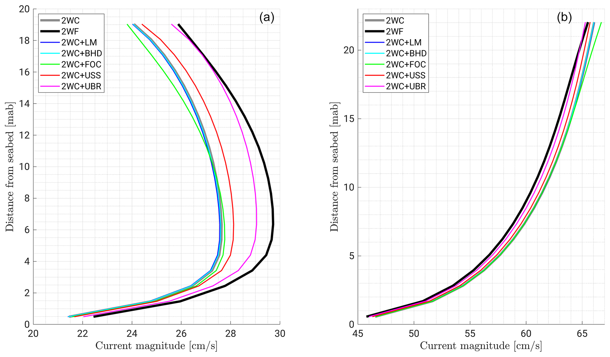
Figure 12 Contributions of the different newly exchanged spectral fields to the vertical current profile in the case of winds coming from the southwest with speeds of the order of 10 m s⁻¹ during tidal ebb (a) and flood (b). Modelled profiles are extracted at the ADCP location on 2 August 2008 at 14:30 (a) and 23:00 (b), corresponding to the profiles shown in Fig. 11.

4.4 Temporal sensitivity to spectral vs. monochromatic wave-induced fields

This section is devoted to the assessment of the impact of spectral versus monochromatic computation of each newly exchanged wave-induced term on the hydrodynamics. Six simulations were performed adding only the exchange of the spectral fields one by one through the coupling interface and then comparing the results in terms of vertical current profiles. Figure 12 shows these comparisons at time instants when the tidal current is affected by wind forcing (also Fig. 11). The profiles predicted by the simulations including only the effect of the spectral mean wavelength (2WC+LM) or the effect of the spectral Bernoulli head (2WC+BHD) match the results of CROCO v1.1 (2WC), indicating that considering these two spectral quantities rather than their monochromatic counterparts does not significantly affect the local hydrodynamics in our configuration. Simulations including only the spectral wave energy dissipation due to breaking (2WC+FOC), the Stokes drift (2WC+USS), or the near-bottom orbital velocity (2WC+UBR) present interesting deviations from that of CROCO v1.1 (2WC). The main effect is caused by the use of spectral near-bed velocity which induces a decrease in the bottom shear stress, leading to an increase in the velocity magnitude in between 1 and 1.5 cm s⁻¹ across the entire water column. The addition of the spectral Stokes drift at the surface and its distribution over the depth according to Eq. (9) slightly changes the vertical shape of the current due to the vortex force, which redistributes the momentum. The velocity magnitude is also altered by the Stokes drift contribution to the vertical advection. Differently, the use of the wave-to-ocean energy flux from the spectral wave model affects the first 5 m below the sea level. This flux represents the wave-breaking contribution to the circulation, which is, in such intermediate depths, associated with whitecapping. It is important to note that in the CROCOv1.1 implementation the wave-to-ocean energy flux is only computed for depth-induced wave breaking, which does not apply here. Consequently, the difference observed here between 2WC and 2WC+FOC shows the added value of including the representation of whitecapping dissipation. With the breaking acceleration force being used for computing and the surface boundary condition for mixing, it is shown to reduce the flow velocity near the surface.

These newly exchanged spectral terms correct the solution predicted by coupling using their monochromatic counterparts when the sea-state spectrum is far from having most of the energy concentrated in one frequency. Figure 13 shows the spectra associated with vertical profiles of Figs. 11 and 12. As expected, the two-peak spectrum (Fig. 13a, c) corresponds to the vertical profile when wind forcing opposes the tidal current (left panel of Fig. 12), which is strongly affected by the spectral versus monochromatic computation of wave-induced terms. Conversely, the one-peak spectrum (Fig. 13b, d) corresponds to the vertical profile when the contributions of the spectral terms are minor (right panel of Fig. 12), as expected.

Figure 13 Wave energy spectra computed by the model at the ADCP location on 2 August 2008 at 14:30 (a, c) and 23:00 (b, d), corresponding to the profiles shown in Figs. 11 and 12. Top panels (a, b) show frequency-direction spectra, while bottom panels (c, d) show frequency spectra integrated over directions.

Differences between the spectral and monochromatic Stokes drifts computed at the ADCP location are shown in Fig. 14 for the entire simulation time. It can be seen that the free-surface (<0.1 m s⁻¹) and depth-averaged (< 0.02 m s⁻¹) values of the Stokes drift are mainly governed by the occurrence of storms, with higher and longer waves associated with larger Stokes velocities (∼0.09 m s⁻¹). The surface Stokes velocity is 2 to 6 times stronger than its barotropic counterpart (2WC and 2WF cases), showing a modulation in time of the vertical shape of the Stokes velocity with the largest changes for strong winds and high waves. The magnitude of the Stokes drift computed by the spectral wave model (2WC, red and magenta lines in Fig. 14) turns out to be smaller than its monochromatic counterpart (2WF, blue and cyan lines in Fig. 14) on 2 August 2008 at 14:30, while spectral and monochromatic values are higher than monochromatic ones on 2 August 2008 at 23:00. Despite the fact that spectral and monochromatic values remain close (only about 1 cm s⁻¹ differences), the impact of the spectral Stokes velocity at the surface on the overall current profile is not negligible, especially at 14:30 as shown in Fig. 14.

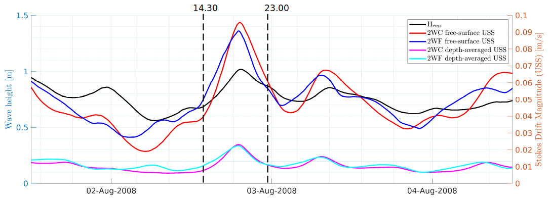
Figure 14 Time series of the modelled magnitude of the Stokes drift at the ADCP location. The black line represents the H_rms. The red and blue lines are the modulus of the free-surface Stokes drift computed by CROCO v1.1 and v1.2, respectively. The magenta and cyan lines are the depth-averaged values of the monochromatic and spectral Stokes drift, respectively.

Differently from the Stokes drift, the near-bottom wave orbital velocity is strongly modulated by the time evolution of the macro-tidal sea-level range (Fig. 15). The near-bed wave orbital velocity is increased during low tide, while a reduction in its intensity is observed during high tide (2WC and 2WF cases). This is primarily due to the fact that in shallower waters the action of waves close to the seabed is enhanced, especially in macro-tidal settings where water depths are of the same order of tidal ranges as at the ADCP location. The modulation according to the tidal phase is more intense for the spectral velocity with an amplification up to 30 %.

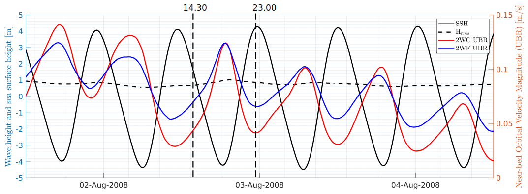
Figure 15 Time series of the modelled magnitude of the near-bed wave orbital velocity at the ADCP location. The black line represents the H_rms, while the dotted line represents the absolute value of the sea surface height. The red and blue lines are the modulus of the near-bed wave orbital velocity computed by CROCO v1.1 and v1.2, respectively.

4.5 Spatial sensitivity to spectral vs. monochromatic wave-induced fields

Differences between the Stokes drift predicted by the spectral model when coupled within the CROCO v1.2 framework (2WF) and its monochromatic approximation computed when coupled within the CROCO v1.1 framework (2WC) are shown for two time instants in the top and bottom panels of Fig. 16. The spectral Stokes drift is accelerated for depth smaller than 5 m, which corresponds to the nearshore and estuarine areas. This acceleration is mainly driven by the water depth and bottom morphology rather than by wind effects because similar patterns are observed at 14:30 and at 23:30. However, the 100 m spatial resolution of the employed computational grid smooths the bathymetry, and thus some key processes such as the depth-induced refraction of waves (e.g. Komen et al., 1994) are likely misrepresented. This low resolution is not appropriate for studying the nearshore dynamics. Off the BoS, a higher spectral-surface Stokes velocity is found with respect to its monochromatic value at the time when the bi-frequency spectrum is observed (14:30). By contrast, at 23:00 the spectral velocity is smaller than the monochromatic one, but the difference is negligible, in line with the observed mono-frequency spectrum. Generally these differences are rather homogeneous across the entire computational domain.

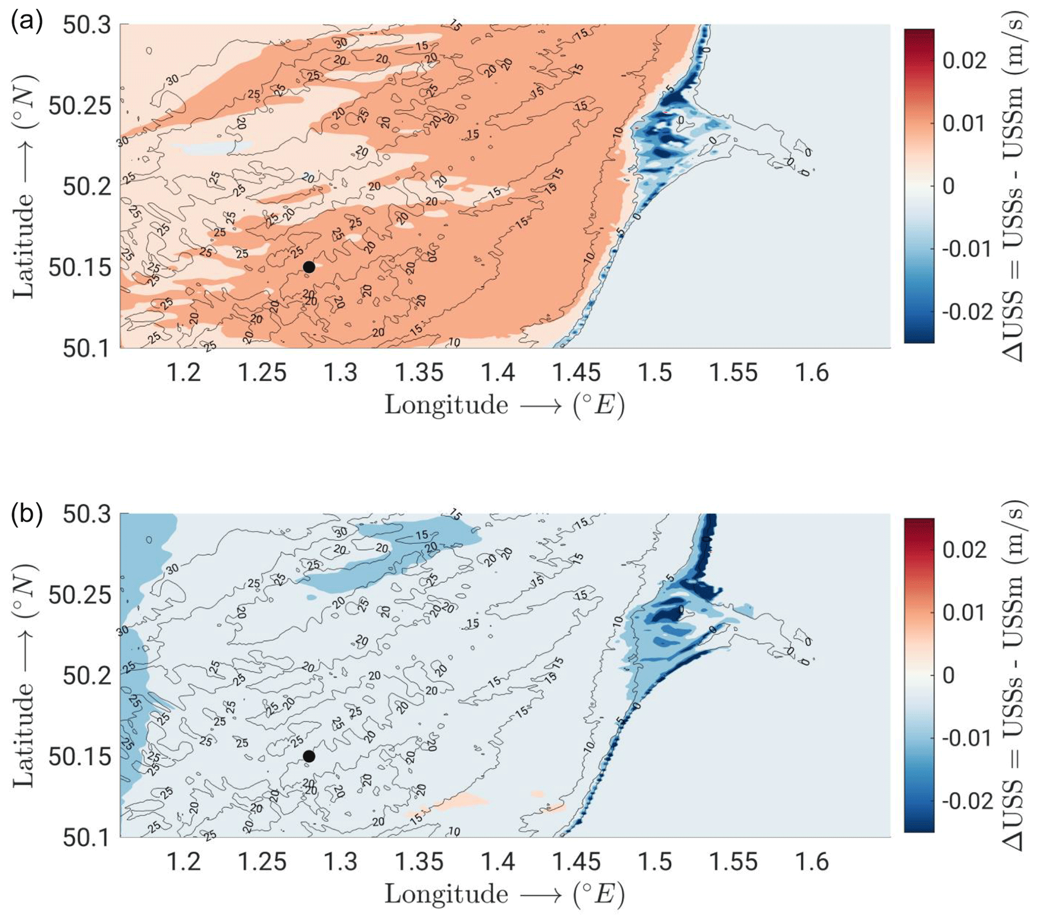
Figure 16 Snapshots of the difference between the spectral (USSs, 2WF) and monochromatic (USSm, 2WC) Stokes drifts computed by CROCO v1.2 and v1.1, respectively, across the whole model domain. Panel (a) shows results at 14:30 on 2 August 2008, while panel (b) shows those at 23:00 on 2 August 2008. ADCP location is marked with a black dot.

The near-bed wave orbital velocity computed by WAVEWATCH-III coupled to CROCO v1.2 (UBRs from run 2WF) and its monochromatic approximation computed by CROCO v1.1 (UBRm from run 2WC) are compared for two time instants (Fig. 17). These results indicate that an increase in spectral near-bottom wave orbital velocity with respect to the monochromatic values is present offshore and mainly depends on the nature of offshore incoming wave spectra and wind forcing. Conversely, and differently from the Stokes drift, bathymetric effects in shallower waters lead to a decrease in spectral wave orbital velocity that reduces to the value predicted by the Airy theory or attains even a smaller value. Also in the case of the wave orbital velocity, the larger differences between spectral and monochromatic values are observed in shallower waters within the bay under both forcing conditions. This confirms that these differences are not only associated with the nature of the forcing spectra, but also with the wave propagation in shallow waters. As mentioned above, the limitations arising from the low horizontal resolution of our computational grid and the omission of wave effects on currents in depths below 2 m hinder our ability to accurately represent wave processes in shallow waters. Consequently, crucial processes influencing near-bottom orbital velocity in the surf zone may not be faithfully captured and need additional dedicated measurements and an increased resolution in this area for a comprehensive investigation.

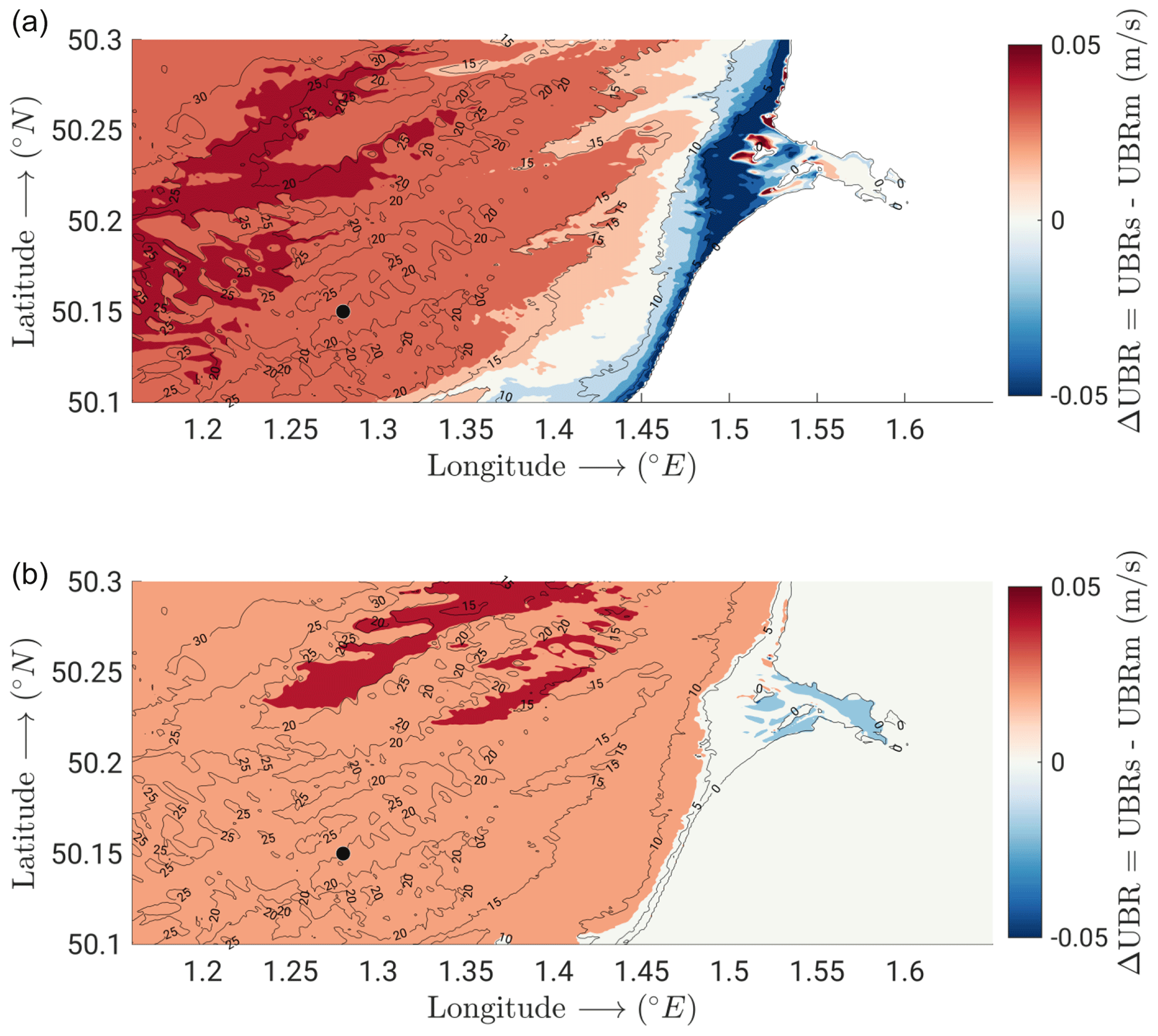
Figure 17 Snapshots of the difference between the spectral (UBRs, 2WF) and monochromatic (UBRm, 2WC) near-bed wave orbital velocity computed by CROCO v1.2 and v1.1, respectively, across the whole model domain. Panel (a) shows results at 14:30 on 2 August 2008, while panel (b) shows those at 23:00 on 2 August 2008. Red marker indicates the ADCP location.

5 Conclusions

In this study we have described the implementation and assessment of an improved coupling (CROCO v1.2) between the oceanic model CROCO and the spectral wave model WAVEWATCH-III, which includes newly exchanged spectral wave fields used to compute wave forcing terms in the wave-averaged governing equations. In addition to significant wave heights, mean wave periods, and directions sent from the wave model to the circulation model in CROCO v1.1, we have added the sending of mean wavelength, near-bottom wave orbital velocity, surface Stokes drift, Bernoulli head, and wave-to-ocean energy flux. Then, these newly exchanged fields are used instead of their monochromatic approximations to compute wave-induced pressure gradients, non-conservative wave effects, and wave-enhanced vertical mixing, including the terms relevant for the surf zone. The impact of using wave forcing terms computed over the full spectrum on the model solutions has been assessed from the coastal dynamic point of view for a coastal configuration of the macro-tidal hydrodynamics off the Bay of Somme, which is dominated by macro-tidal currents that are influenced by storm winds and waves.

Model results have been compared against those of an existing wave model and in situ wave and current measurements. Modelled waves are on average of the right order of magnitude, but minimum heights are overestimated and maximum heights are underestimated, and a phase shift is observed throughout the whole simulated time series. The biases are, however, similar to those of the wave hindcast used to force the model boundaries, which also uses similar parameterizations. These biases may thus be attributed to their propagation from the boundaries and/or parameterization setup. Differently, the fair matching between modelled water levels and currents with both current measurements from punctual (AQDP) and profiler (ADCP) current metres validates the new numerical developments in the circulation model. The modelled hydrodynamics well captures the macro-tidal range off the bay. Sensitivity experiments for the forcing indicate that metocean conditions do not significantly affect water levels and near-bottom currents that are primarily dominated by tides. Conversely, wind- and wave-induced effects are found to regulate the currents at the free surface. Here, storm winds blowing onshore accelerate flood flows and decelerate ebb flows, modifying the overall logarithmic vertical profile of tidal currents. Concurrently, storm waves act to decrease the surface-wind-driven acceleration, smoothing the vertical current profile throughout the entire water column. Modelled currents are correctly predicted during most of the phases of the tidal cycle, particularly at current reversal. Only at the peak of tidal floods is a small phase shift between modelled and measured currents observed. However, this slight periodic mismatch does not appear related to changing wind and wave conditions. It is thus not considered as a hindrance to the evaluation of our model developments, which focus on wind and wave influences on macro-tidal currents at intermediate water depths.

The additional spectral-wave-induced terms significantly affect the results in the case of storm waves and winds opposed to tidal flows, reducing the wave-induced deceleration of the vertical profile of tidal currents. Their contributions provide current magnitudes closer to measurements than those predicted using their monochromatic formulations, particularly at the free surface. Their inclusion in the fully coupled model introduced a negligible computational cost increase, accounting for less than 1 % of the total computational time compared to the previous version of the coupled model. However, it should be noted that this assessment pertains to the present model configuration with a limited domain extension, and further evaluation may be necessary for larger model domains.

In the particular case of the Bay of Somme, flood (ebb) surface currents are overestimated (underestimated) during passing storms when approximating these spectral fields with their monochromatic counterparts. The error associated with this approximation is the largest when winds and tidal flows are opposed and when the wave spectrum is not mono-modal. Among the investigated additional spectral-wave-induced terms, the surface Stokes drift and the near-bed wave orbital velocity are the ones with the most impact. The spectral Stokes drift leads to an increased advection towards the free surface, while the spectral near-bed wave orbital velocity leads to a shifting of the vertical profile of currents close to the seabed. Their importance is also thought to increase towards shallow waters where winds and waves dominate the nearshore circulation, with implications on air–sea interactions and sediment transport processes. As such, our model development provides a better description of the competing effects of tides, winds, and waves on the oceanic circulation in coastal macro-tidal areas and is now available in CROCO v1.2 for future studies.