GLOBGM v1.0: a parallel implementation of a 30 arcsec PCR-GLOBWB-MODFLOW global-scale groundwater model

We discuss the various performance aspects of parallelizing our transient global-scale groundwater model at 30^′′ resolution (30 arcsec; ∼ 1 km at the Equator) on large distributed memory parallel clusters. This model, referred to as GLOBGM, is the successor of our 5^′ (5 arcmin; ∼ 10 km at the Equator) PCR-GLOBWB 2 (PCRaster Global Water Balance model) groundwater model, based on MODFLOW having two model layers. The current version of GLOBGM (v1.0) used in this study also has two model layers, is uncalibrated, and uses available 30^′′ PCR-GLOBWB data. Increasing the model resolution from 5^′ to 30^′′ creates challenges, including increased runtime, memory usage, and data storage that exceed the capacity of a single computer. We show that our parallelization tackles these problems with relatively low parallel hardware requirements to meet the needs of users or modelers who do not have exclusive access to hundreds or thousands of nodes within a supercomputer.

For our simulation, we use unstructured grids and a prototype version of MODFLOW 6 that we have parallelized using the message-passing interface. We construct independent unstructured grids with a total of 278 million active cells to cancel all redundant sea and land cells, while satisfying all necessary boundary conditions, and distribute them over three continental-scale groundwater models (168 million – Afro–Eurasia; 77 million – the Americas; 16 million – Australia) and one remaining model for the smaller islands (17 million). Each of the four groundwater models is partitioned into multiple non-overlapping submodels that are tightly coupled within the MODFLOW linear solver, where each submodel is uniquely assigned to one processor core, and associated submodel data are written in parallel during the pre-processing, using data tiles. For balancing the parallel workload in advance, we apply the widely used METIS graph partitioner in two ways: it is straightforwardly applied to all (lateral) model grid cells, and it is applied in an area-based manner to HydroBASINS catchments that are assigned to submodels for pre-sorting to a future coupling with surface water. We consider an experiment for simulating the years 1958–2015 with daily time steps and monthly input, including a 20-year spin-up, on the Dutch national supercomputer Snellius. Given that the serial simulation would require ∼ 4.5 months of runtime, we set a hypothetical target of a maximum of 16 h of simulation runtime. We show that 12 nodes (32 cores per node; 384 cores in total) are sufficient to achieve this target, resulting in a speedup of 138 for the largest Afro–Eurasia model when using 7 nodes (224 cores) in parallel.

A limited evaluation of the model output using the United States Geological Survey (USGS) National Water Information System (NWIS) head observations for the contiguous United States was conducted. This showed that increasing the resolution from 5^′ to 30^′′ results in a significant improvement with GLOBGM for the steady-state simulation when compared to the 5^′ PCR-GLOBWB groundwater model. However, results for the transient simulation are quite similar, and there is much room for improvement. Monthly and multi-year total terrestrial water storage anomalies derived from the GLOBGM and PCR-GLOBWB models, however, compared favorably with observations from the GRACE satellite. For the next versions of GLOBGM, further improvements require a more detailed (hydro)geological schematization and better information on the locations, depths, and pumping rates of abstraction wells.

1 Introduction

The PCRaster Global Water Balance model (PCR-GLOBWB; van Beek et al., 2011) is a grid-based, global-scale hydrology and water resource model for the terrestrial part of the hydrologic cycle that was developed at the Utrecht University, the Netherlands. This model, using a Cartesian (regular) grid representation for the geographic coordinate system (latitude and longitude), covers all continents, except Greenland and Antarctica. For more than a decade, it has been applied to many water-related global change assessments providing estimates and future projections, e.g., regarding drought and groundwater depletion due to non-renewable groundwater withdrawal (Wada et al., 2010; de Graaf et al., 2017).

The latest version of PCR-GLOBWB (version 2.0; Sutanudjaja et al., 2018), or PCR-GLOBWB 2, has a spatial resolution of 5^′ (5 arcmin) corresponding to ∼ 10 km at the Equator. It includes a 5^′ global-scale groundwater model based on MODFLOW (Harbaugh, 2005), consisting of two model layers to account for confining, confined, and unconfined aquifers (de Graaf et al., 2015, 2017). Recent publications have called for a better representation of groundwater in Earth system models (Bierkens, 2015; Clark et al., 2015; Gleeson et al., 2021). Apart from providing a globally consistent and physically plausible representation of groundwater flow, global-scale groundwater models could serve to support global change assessments that depend on a global representation of groundwater resources. Examples of such assessments are the impact of climate change on vegetation, evaporation and atmospheric feedbacks (Anyah et al., 2008; Miguez-Macho and Fan, 2012), the role of groundwater depletion in securing global food security and trade (Dalin et al., 2017), and the contribution of terrestrial water storage change to regional sea level trends (Karabil et al., 2021). From the work of de Graaf et al. (2017) and recent reviews (Condon et al., 2021, and Gleeson et al., 2021), it follows that a number of steps is needed to make the necessary leap change in improving the current generation of global-scale groundwater models. Specifically, these are (1) improved hydrogeological schematization, particularly including multilayer semi-confined aquifer systems and the macroscale hydraulic properties of karst and fractured systems; (2) increased resolution to better resolve topography and, in particular, to resolve smaller higher-altitude groundwater bodies in mountain valleys; (3) improved knowledge on the location, depth, and rate of groundwater abstractions; (4) better estimates of groundwater recharge, especially in drylands and at mountain margins; and (5) increased computational capabilities to be able to make simulations with the abovementioned improvements possible. Our paper specifically revolves around items (2) and (5) and focuses on the following research question: if we improve spatial resolution, how should we make this computationally possible? It is a small but necessary and important step to better global-scale groundwater simulation that needs to be taken to proceed further.

Here, we therefore consider a spatially refined version of the 5^′ PCR-GLOBWB-MODFLOW global-scale groundwater model to 30^′′ resolution (∼ 1 km at the Equator), referred to as GLOBGM in the following. The initial version of GLOBGM, v1.0 that we developed in this study, has a maximum of two model layers and uses refined input from available PCR-GLOBWB simulations and the native parameterization of the global-scale groundwater model of de Graaf et al. (2017). Since we focus on the abovementioned research question to improve spatial resolution, we note that improving the schematization and parameterization is left for further research and for future versions of GLOBGM.

Pushing forward to a 30^′′ resolution is a direct result of the growing availability of high-resolution data sets and the wish to exploit the benefits of high-performance computing (HPC) to maximize computer power and modeling capabilities (Wood et al., 2011; Bierkens et al., 2015). Typically, high-resolution digital elevation maps (DEMs) are available, as derived from NASA Shuttle Radar Topography Mission products such as HydroSHEDS (Lehner et al., 2008) at 30^′′ or the MERIT DEM (Yamazaki et al., 2017) at even 3^′′. Furthermore, subsurface data are becoming available in a higher resolution, such as gridded soil properties at 250 m resolution from SoilGrids (Hengl et al., 2014) and global lithologies for ∼ 1.8 million polygons from GLHYMPS (Huscroft et al., 2018). Although Moore's law still holds, viz. stating that processor performance doubles every 2 years, more and more processor cores are being added to increase performance. This means that making software suitable for HPC inevitably requires efficient use of the available hardware. Anticipating this, we parallelized the groundwater solver for GLOBGM, as well as the pre-processing.

In this paper, the focus is on the technical challenges of implementing GLOBGM using HPC given a performance target. The focus is not on improving schematization and/or parameterization, and we use available PCR-GLOBWB data only. Furthermore, this study is mainly focusing on transient simulation, since transient simulations make the most sense for evaluating the effects of climate change and human interventions (see, e.g., Minderhoud et al., 2017). We apply a similar approach to de Graaf et al. (2017) to obtain initial conditions for GLOBGM; we use a steady-state result (under natural conditions; no pumping) to spin-up the model by running the first year back-to-back for 20 years to reach dynamic equilibrium. We restrict ourselves to presenting parallel performance results for transient runtimes only, since we found that steady-state runtimes with GLOBGM are negligible compared to transient runtimes. We present a parallelization methodology for GLOBGM and illustrate this by a transient experiment on the Snellius Dutch national supercomputer (SURFsara, 2021) for simulating the period 1958–2015 (58 years), including a 20-year spin-up. We provide a limited evaluation of the computed results, and we note that the current model is a first version that should be further improved in the future. We refer to Gleeson et al. (2021) for an extensive discussion on pathways to further evaluate and improve global-scale groundwater models. For this, the steady-state and transient results with GLOBGM are compared to hydraulic head observations for the contiguous United States (CONUS), also considering the 5^′ PCR-GLOBWB global-scale groundwater model, the 30^′′ global-scale inverse model of Fan et al. (2017), and the 250 m groundwater model for the CONUS of Zell and Sanford (2020). Furthermore, we compare simulated monthly and multi-year total water storage anomalies calculated with the GLOBGM and PCR-GLOBWB models, with observations from the Gravity Recovery and Climate Experiment satellite (GRACE) and its follow-on mission (Wiese, 2015; Wiese et al., 2016).

We use the model code program MODFLOW (Langevin et al., 2021, 2017), the most widely used groundwater modeling program in the world, developed by the U.S. Geological Survey (USGS). The latest version 6 of MODFLOW supports a multi-model functionality that enable users to set up a model as a set of (spatially non-overlapping) submodels, where each submodel is tightly connected to other submodels at matrix level and has its own unique set of input and output files. In cooperation with the USGS, we parallelized this submodel functionality and created a prototype version (Verkaik et al., 2018, 2021c) that is publicly available and is planned to be part of a coming MODFLOW release. Building on our preceding research (Verkaik et al., 2021a, b), this prototype uses the message-passing interface (MPI; Snir et al., 1998) to parallelize the conjugate gradient linear solver within the iterative model solution package (Hughes et al., 2017), supporting the additive Schwarz preconditioner and the additive coarse-grid-correction preconditioner (Smith et al., 1996).

This paper is organized as follows. First, the general parallelization approach for implementing GLOBGM is given in Sect. 2.1, followed by the experimental setup in Sect. 2.2, the workflow description in Sect. 2.3, and model evaluation methods in Sect. 2.4. Second, the results are presented and discussed for the transient pre-processing in Sect. 3.1, the transient parallel performance in Sect. 3.2, the model evaluation in Sect. 3.3, and some examples of global-scale results are given in Sect. 3.4. Finally, Sect. 4 concludes this paper.

2 Methods

2.1 Parallelization approach

2.1.1 General concept

The 5^′ PCR-GLOBWB-MODFLOW global-scale groundwater model (GGM) consists of two model layers; where a confining layer (with lower permeability) is present, the upper model layer represents the confining layer, and the lower model layer a confined aquifer. If a confining layer is not present, then both the upper and lower model layers are part of the same unconfined aquifer (de Graaf et al., 2017, 2015). The GGM uses a structured Cartesian grid (geographic projection), representing latitude and longitude, and includes all land and sea cells at the global 5^′ extent. Using such a grid means that we have to take into account the fact that cell areas and volumes do vary in space, and therefore, the MODFLOW input for the recharge and the storage coefficient need be corrected for this (see Sutanudjaja et al., 2011, and de Graaf et al., 2015, for details). Each of the two GGM layers has 9.3 million 5^′ cells (4320 columns times 2160 rows), and therefore, the GGM has a total of ∼ 18.7 million 5^′ cells. A straightforward refinement of this grid to 30^′′ resolution would result in ∼ 100 times more cells and hence 1.87 billion cells (two model layers of 43 200 columns times 21 600 rows). Creating and using such a model would heavily stress the runtime, memory usage, and data storage.

To address this problem, we can significantly reduce the number of grid cells by applying unstructured grids and maximizing parallelism by deriving as many independent groundwater models as possible, while satisfying all necessary boundary conditions. This concept is illustrated by Fig. 1. Starting with the 30^′′ global-scale land–sea mask and boundary conditions prescribed by the GGM, we first derive independent unstructured grids and group them in a convenient way from large to small (see Sect. 2.1.2 for details). Then, we define GLOBGM as a set of four independent groundwater models: three continental-scale groundwater models for the three largest unstructured grids and one remaining model called the “Island model” for the remainder of the smaller unstructured grids (see Sect. 2.1.3 for details). The unstructured grids for these defined models are subject to parallelization; there are two partitioning methods (or domain decomposition methods) considered (see Sect. 2.1.4 for details), with one for partitioning grid cells straightforwardly (gray arrows in Fig. 1) and the other for partitioning water catchments (red arrows in Fig. 1). For each groundwater model, the chosen partitioning results in non-overlapping subgrids that define the computational cells for the non-overlapping groundwater submodels, where the computational work for each submodel is uniquely assigned to a processor core (MPI rank). Note that we deliberately reserve the term “submodel” and “subgrid” for parallel computing. It should also be noted that deriving independent groundwater models as we do in our approach could, in principle, also be executed for structured grids. However, this would introduce a severe overhead of redundant cells for each independent groundwater model. Furthermore, in that case, defining the Islands model would virtually make no sense, since islands are scattered globally, and the structured grid for this model would be therefore almost as large as the one for the entire model.

In this work, we focus on solving the groundwater models of GLOBGM using distributed memory parallel computing (Rünger and Rauber, 2013). We restrict ourselves to parallelization on mainstream cluster computers, since they are often accessible to geohydrological modelers. Cluster computers typically have distributed memory (computer) nodes, where each node consists of several multicore central processing units (CPUs; sockets) sharing memory, and each node is tightly connected to other nodes by a fast (high-bandwidth and low-latency) interconnection network. Instead of focusing on parallel speedups and scalability, which are commonly used and valuable metrics for benchmarking parallel codes (e.g., Burstedde et al., 2018), we focus on a metric that we believe is meaningful to the typical user for evaluating transient groundwater simulations, namely the simulated years per day (SYPD). This metric, simply the number of years that a model can be simulated in a single day of 24 h, has proven to be useful for evaluating the massively parallel performance in the field of atmospheric community modeling (Zhang et al., 2020).

Choosing a target performance R_tgt in SYPD, we conduct a strong scaling experiment to estimate the number of cores and nodes to meet this target. To do so, we select a representative but convenient groundwater model of GLOBGM and determine the number of nodes to meet R_tgt for a pre-determined maximum number of cores per node and a short period of simulation. Then, the target submodel size (grid cell count) is determined and used straightforwardly to derive the number of cores and nodes for all of the groundwater models of GLOBGM (see Sect. 2.1.5 for details). In the most ideal situation, using these estimates for the number of cores and nodes would result in a parallel performance that meets the target performance R_tgt for each of the four groundwater models of GLOBGM.

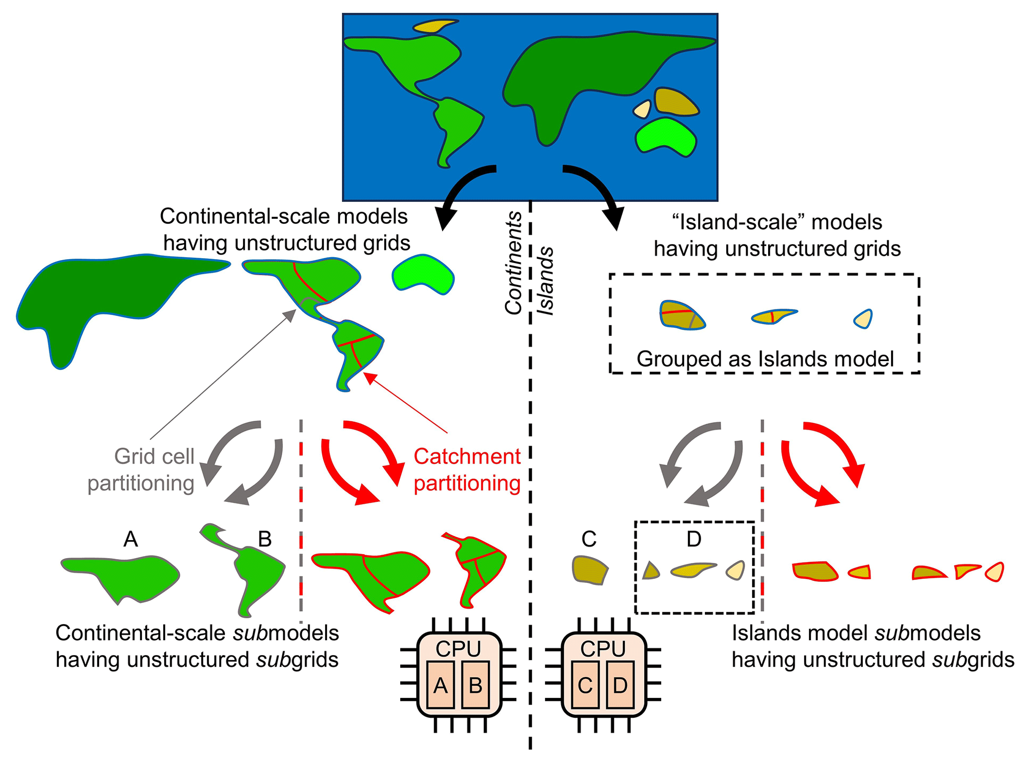
Figure 1 General concept of defining GLOBGM as a set of independent (larger) continental-scale groundwater models (left-hand side) and (smaller) island-scale groundwater models as a remaining model (right-hand side). All of these models have independent unstructured grids that are partitioned by (a) straightforwardly assigning grid cells (grid cell partitioning; gray arrows) or (b) assigning catchments (catchment partitioning; red arrows). The resulting subgrids define the computational cells for the submodels that are uniquely assigned to a processor core/MPI process. In this figure, this is illustrated by assigning submodels “A” and “B” to one dual-core CPU and submodels “C” and “D” to another.

2.1.2 Procedure for deriving the independent unstructured grids

The starting point of the unstructured grid generation is a 30^′′ global-scale land–sea mask. Within the GGM, continents and islands are numerically separated (no implicit connection) by the sea cells and more precisely by a lateral Dirichlet boundary condition (BC) of a hydraulic head of 0 m for land cells near the coastline. Since this BC is only required near the coastline, this means that ∼ 77 % of the 5^′ grid cells corresponding to sea are redundant. This motivates the application of unstructured grids for grid cell reduction. Using the 30^′′ mask, first, a minimal number of sea cells is added to the land cells in the lateral direction to provide for the Dirichlet BC by applying an extrapolation using a five-point stencil. Second, from this resulting global map, all independent and disjoint continents/islands are determined, each having a (an augmented) land–sea mask. Using this land mask, the unstructured grid generation is done to account for the absence of the confining layer, where the GGM uses zero-thickness (dummy) cells for the upper layer as a workaround for specifying a lateral homogeneous Neumann BC (no-flow). This holds for ∼ 35 % of the land cells of the GGM, also motivating the usage of unstructured grids for grid cell reduction. This means that in GLOBGM the following two subsurface configurations are used: (1) an upper confining layer plus lower confined aquifer (2 vertical cells) and (2) an (a lower) unconfined aquifer (one vertical cell). For the sake of convenience, we sometimes use “upper model layer” and “confining layer” interchangeably, as well as “lower model layer” and “aquifer”. Note that in GLOBGM, interaction with surface water or surface drainage is modeled by putting rivers and drains in the first active layer, as seen from top to bottom.

The resulting grids in GLOBGM are clearly unstructured, since the number of cell neighbors is not constant for all grid cells; therefore, the grid cell index cannot be computed directly. In the lateral direction, constant-head cells (Dirichlet; 0 m) near the coastal shore are not connected to any neighboring canceled sea cells, and in the vertical direction, we cannot distinguish between the upper and lower model layer anymore due to the canceling of non-existing upper confining layer cells. Because of this, we apply the Unstructured Discretization (DISU) package with MODFLOW (Langevin et al., 2017).

As a result of our procedure, we get N_g=9050 independent unstructured grids, thus corresponding to 9050 independent groundwater models, for a total of ∼ 278.3 million 30^′′ grid cells. Compared to the straightforward structured grid refinement of the GGM to 30^′′ resolution resulting in 1.87 billion grid cells (see Sect. 2.1.1), these unstructured grids give an 85 % cell reduction (land has a 35 % reduction; sea has a 99.9 % reduction). As a final step, we sort the unstructured grids by cell count, resulting in g_n, $n=\mathrm{1},\mathrm{\dots },N_g$ grids, since this is convenient for identifying the largest and most computationally intensive groundwater models subject to parallelization.

2.1.3 Defining the four groundwater models of GLOBGM

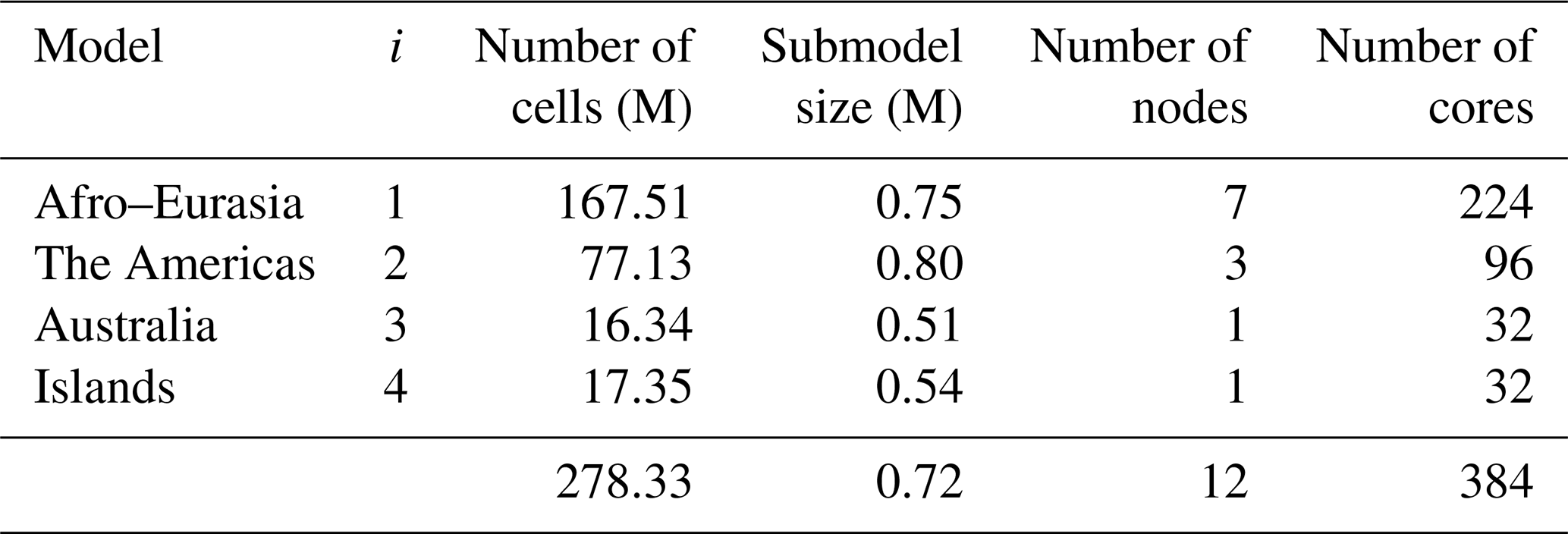
Although, from a modeling perspective, we might use all the 9050 derived independent groundwater models for GLOBGM that result from the procedure mentioned above (Sect. 2.1.2), we limit the number models for the sake of coarse-grain parallelization and the simplification of data management. Choosing a maximum of four (N_m=4), the computational cells for the three largest models are defined by unstructured grids g₁, g₂ and g₃, respectively: Afro–Eurasia (AE; 168 million 30^′′ cells), the Americas (AM; 77 million 30^′′ cells), and Australia (AU; 16 million 30^′′ cells). The remaining 9047 smaller grids, $g_{\mathrm{4}},\mathrm{\dots },g_{\mathrm{9050}}$, with total of 17 million 30^′′ cells, are grouped as Islands (ISL; see Fig. 2). By doing this, we define GLOBGM as a set of four independent groundwater models that are subject to parallelization, of which three of them are continental-scale groundwater models, and one is the remaining model for the smaller islands (Islands model). The maximum of four is motivated by the observation that the Islands model has almost the same number of cells as the Australia model, and therefore, we do not feel any need to use more groundwater models.

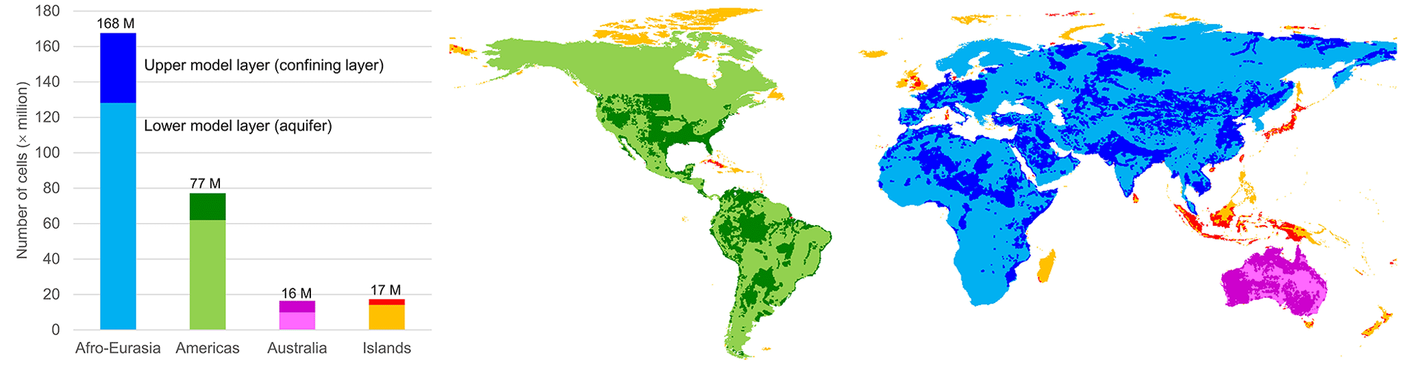
Figure 2 The four defined model areas of GLOBGM with a total of 278.3 million cells. When the upper model layer is plotted, this means that there is also a lower model layer present. Otherwise, only the lower model layer is present.

2.1.4 Groundwater model partitioning: grid cell partitioning and catchment partitioning

To parallelize GLOBGM, each of the four groundwater models is partitioned into multiple non-overlapping groundwater submodels, where each groundwater submodel is uniquely assigned to one processor core and one MPI process. To obtain a good parallel performance, the computational work associated with the submodels should be well balanced. For this reason, we perform a grid partitioning using METIS (Karypis and Kumar, 1998), the most commonly used graph partitioner among others like Chaco (Hendrickson and Leland, 1995) and Scotch (Pellegrini, 2008). Input for this partitioner is an undirected graph, consisting of (weighted) vertices and edges and the desired number of partitions. Here, we restrict our grid partitioning to lateral direction only, since the number of lateral cells is much larger than the number of model layers (here a maximum of two). This naturally minimizes the number of connections between the submodels and the associated point-to-point (inter-core) MPI communication times.

For each model mⁱ, $\mathrm{1}\le i\le N_m$, a set of (coupled) submodels as a result of partitioning is defined by m^i,j, $j=\mathrm{1},\mathrm{\dots },N_m^i$, where $N_m^i$ is the number of submodels for model i. In our approach, each submodel is constructed by combining one or more areas $a_k^{i,j}$, $k=\mathrm{1},\mathrm{\dots },N_a^{i,j}$, where $N_a^{i,j}$ is the number of areas for model i, which is the submodel j of model i. Here, an area is defined as a 2D land surface represented by laterally connected, non-disjoint 30^′′ grid cells. The total number of areas for a model is defined by $N_a^i={\sum }_j{N}_a^{i,j}$ and for the entire GLOBGM by $N_a={\sum }_i{N}_a^i$. The general approach is to assign one or more areas to a submodel using METIS. Hereafter, we refer to this as area-based graph partitioning. To that end, two partitioning strategies are considered, using the following:

1. METIS areas that are generated by straightforwardly applying METIS to model grids for mⁱ to obtain $N_m^i$ parts. We refer to this as the (straightforward) grid cell partitioning.

2. Catchment areas that are generated by the rasterization and extrapolation of HydroBASINS catchments, including lakes (Lehner and Grill, 2013). HydroBASINS catchments follow the Pfafstetter base 10 coding system for hydrologically coding river basins, where the main stem is defined as the path which drains the greatest area, and at each refinement level, 10 areas are defined, namely four major tributaries, five inter-basin regions, and one closed drainage system (Verdin and Verdin, 1999). We refer to this as the catchment partitioning.

For straightforward grid cell partitioning, we restrict ourselves to assigning exactly one METIS area to a submodel; hence, $N_a^{i,j}=\mathrm{1}$ for all j. In this approach, each lateral grid cell of model mⁱ is subject to the METIS partitioner; each vertex in the graph corresponds to a lateral cell having a vertex weight equal to the number of vertical cells (1 or 2), and each edge corresponds to the inter-cell connection having an edge weight of 1 or 2, depending on the number of neighboring model layers. For catchment partitioning, typically $N_a^{i,j}\gg \mathrm{1}$, each vertex in the METIS graph represents a catchment area; each vertex in the graph has a weight equal to the total number of grid cells within that catchment, and each edge corresponds to the inter-catchment connection having an edge weight equal to the sum of inter-cell connections to neighboring catchments.

Compared to straightforward grid cell partitioning, the graph being used by catchment partitioning is much smaller than the graph used by grid cell partitioning, since the number of catchments is generally much smaller than the number of lateral cells. Therefore, the METIS solver has much fewer degrees of freedom and is generally less optimal for catchment partitioning. However, catchment partitioning has several advantages compared to grid cell partitioning. First, the graphs are generally much smaller, and therefore, partitioning is significantly faster. In fact, this approach makes the grid partitioning almost independent of the grid cell resolution and is therefore suitable for even higher resolutions in the future. Second, catchment partitioning gives users the flexibility to give the lateral submodel boundaries physical meaning. For example, choosing catchment boundaries simplifies a future parallel coupling to surface water routing modules (Vivoni et al., 2011). Third, this concept could be easily generalized for other types of areas, e.g., countries or states following administrative boundaries. Choosing such areas might simplify the management and maintenance of the submodels by different stakeholders within a community model.

Figure 3 illustrates the defined model entities for the case of one continent and three islands (N_g=4), two models (N_m=2), and seven catchments areas (N_a=7). In this example, model m¹ has the largest (unstructured) grid g₁, and model m² has the remaining smaller (unstructured) grids g₂,g₃, and g₄. The denoted cell numbers in Fig. 3 correspond to the numbers of model layers, where blue denotes a cell with a Dirichlet (sea) BC. In this example, each model has exactly two submodels (hence, $N_m^{\mathrm{1}}=N_m^{\mathrm{2}}=\mathrm{2})$. For model m¹, catchments $a_{\mathrm{1}}^{\mathrm{1},\mathrm{1}}$ and $a_{\mathrm{2}}^{\mathrm{1},\mathrm{1}}$ are assigned to submodel m^1,1, and $a_{\mathrm{1}}^{\mathrm{1},\mathrm{2}}$ is assigned to submodel m^1,2. For model m², catchment $a_{\mathrm{1}}^{\mathrm{2},\mathrm{1}}$ is assigned to submodel m^2,1, and $a_{\mathrm{1}}^{\mathrm{2},\mathrm{2}}$, $a_{\mathrm{2}}^{\mathrm{2},\mathrm{2}}$, and $a_{\mathrm{3}}^{\mathrm{2},\mathrm{2}}$ are assigned to submodel m^2,2. For this example, the load of model m¹ is well-balanced, since each submodel has a load of 50. However, for model m², the first and second submodel have load 19 and 21, respectively, and therefore, there is a load imbalance. Note that submodel m^2,2 has three disjoint subgrids, since in this case three islands are involved. This outlined situation for model m², where a submodel can have multiple disjoint subgrids, may occur in the global domain decomposition for the Islands model, since grid cell partitioning is done for all 9047 disjoint grids together. In general, the presence of disjoint subgrids may occur for any submodel within GLOBGM, also for the Afro–Eurasia, the Americas, and Australia models. The reason is that none of the METIS solvers can guarantee contiguous partitions. However, we here use the multilevel recursive bisection option that is known to give best results in that respect.

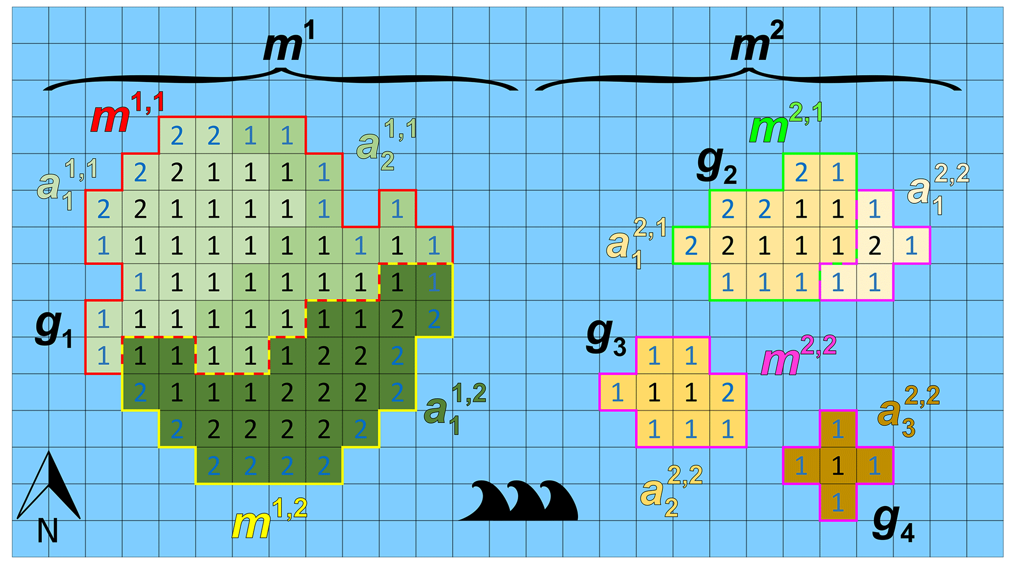
Figure 3 Example of an imaginary world containing one large continent in the west (with an unstructured grid g₁) and three smaller islands in the east (with unstructured grids g₂, g₃, and g₄ from smallest to largest). The world's model is chosen to be a set of two models, namely one continental-scale model m¹(g₁) and one Islands model m²(g₂, g₃, and g₄). In this example, each of the models consists of exactly two submodels that are determined using catchment partitioning (strategy 2): for model m¹, catchments $a_{\mathrm{1}}^{\mathrm{1},\mathrm{1}}$ and $a_{\mathrm{2}}^{\mathrm{1},\mathrm{1}}$ are assigned to submodel m^1,1 and $a_{\mathrm{1}}^{\mathrm{1},\mathrm{2}}$ to submodel m^1,2. For model m², catchments $a_{\mathrm{1}}^{\mathrm{2},\mathrm{1}}$ and $a_{\mathrm{1}}^{\mathrm{2},\mathrm{2}}$ are assigned to submodel m^2,1 and $a_{\mathrm{2}}^{\mathrm{2},\mathrm{2}}$ and $a_{\mathrm{3}}^{\mathrm{2},\mathrm{2}}$ to submodel m^2,2. Note that in this example model, m² is the remaining model and is chosen to consists of three islands that each could have been chosen as a separate independent model. Furthermore, note that for this model m², submodel m^2,2 consists of three disjoint subgrids. The numbered cells denote the cells included in the model because the number equals the number of vertical cells, and blue numbers denote constant head (Dirichlet) cells with a head of 0 m.

2.1.5 Node selection procedure

When evaluating the target performance R_tgt, we restrict ourselves to model runtime only. Since pre- and post-processing are very user-specific, associated runtimes cannot be generalized. However, we do consider them in our analysis. Processing runtimes can be substantial, making parallel processing inevitable, as we will illustrate for our limited pre-processing. To keep pre-processing runtimes feasible, we apply embarrassing parallelization (see e.g.,  Eijkhout et al., 2015 ), where processing for input data (tiles and submodels) is done independently, using multiple threads simultaneously on multiple nodes.

To achieve R_tgt, we need a selection procedure for estimating the number of (processor) cores for the three continental-scale groundwater models and the Islands model. Since it is common to take the number of cores per node at a fixed value (N_CPN), this means that choosing the number of cores is equivalent to choosing the number of nodes. Ideally, we would take N_CPN to be equal to the total number of cores within a node and therefore maximize computer resource utilization. However, it is not always advantageous to use the total number of cores, due to the memory access constraint, or sometimes not even possible when the memory required for the associated submodels exceeds the available memory within a node. In practice, the best performance is often obtained using a smaller number of cores. For example, the linear conjugate gradient solver that is used for solving the groundwater flow equation dominates runtime and is strongly memory-bound because of the required sparse matrix–vector multiplications (Gropp et al., 1999). This means that, starting from a certain number of cores, the competition for memory bandwidth hampers a parallel performance, and contention is likely to occur (Tudor et al., 2011). Typically, this directly relates to the available memory channels within a multicore CPU, linking the RAM (random access memory) and processor cores. In our approach, we first determine N_CPN by performing a strong scaling experiment (keeping the problem size fixed) within a single node for the well-known high-performance conjugate gradients supercomputing benchmark (HPCG; Dongarra et al., 2016). By doing this, we assume that HPCG is representative of the computation in MODFLOW. The performance metric for this experiment is the floating-point operations per second (FLOPS) that is commonly used for quantifying numerical computing performance and processor speed. Then, by conducting a strong scaling experiment for a single (medium-sized) model and a short simulation period, while keeping N_CPN fixed, the number of nodes is selected such that R_tgt is achieved. This gives the preferred submodel size that is used to determine the number of nodes for all other models (see Sect. 2.3.1 for more details).

2.2 Experimental setup

2.2.1 Description of GLOBGM and application range

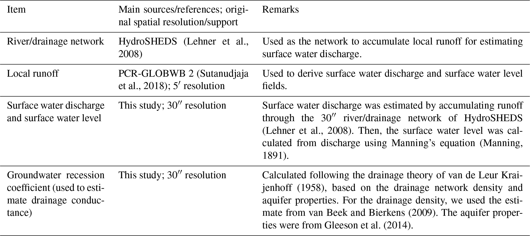
Tables 1 and 2 show the data sets used to parameterize GLOBGM in this study. For details on the MODFLOW model description and conceptualization, we refer to the preceding research (de Graaf et al., 2019, 2017, 2015; Sutanudjaja et al., 2014, 2011). The application domain of GLOBGM is similar to that of the 5^′ PCR-GLOBWB global-scale groundwater model (GGM; de Graaf et al., 2017). We therefore note that the limitations of the GGM also apply to GLOBGM. For clarity, we repeat these limitations here: (1) the GGM is intended to simulate hydraulic heads in the top aquifer systems, meaning unconfined aquifers and the uppermost confining aquifers; (2) wherever there are multiple stacked aquifer systems, these are simplified in the model to one confining layer and one confined aquifer; (3) the model schematization is suitable for hydraulic heads in large sedimentary alluvial basins (main productive aquifers) that have been mapped at a 5^′ resolution; (4) in as far as these sedimentary basins include karst, it is questionable if a Darcy approach can be used to simulate large-scale head distributions; (5) due to the limited resolution of the hydrogeological schematizations, in mountain areas we simulate the hydraulic heads in the mountain blocks but not those of groundwater bodies in hillslopes and smaller alluvial mountain valleys; and (6) also, for the hydraulic heads in the mountain blocks, we assume that secondary permeability of fractured hard rock can also simulated with Darcy groundwater flow, which is an assumption that may be questioned.

In this study, we adopted an offline coupling approach that used the PCR-GLOBWB model output of Sutanudjaja et al. (2018) as the input to the MODFLOW groundwater model. The PCR-GLOBWB model output that was used consists of monthly fields for the period 1958–2015 for the variable groundwater recharge (i.e., net recharge obtained from deep percolation and capillary rise), groundwater abstraction, and runoff. The latter was translated to monthly surface water discharge by accumulating it through the 30^′′ river/drainage network of HydroSHEDS (Lehner et al., 2008). From the monthly surface water discharge fields, we then estimated surface water levels using Manning's equation (Manning, 1891) and the surface water geometry used in the PCR-GLOBWB model.

The groundwater model simulation conducted consists of two parts: a steady-state and a transient simulation. For both simulations, default solver settings from the 5^′ model were taken for evaluating convergence, and within the linear solver, we did not apply coarse-grid correction. We started with a steady-state MODFLOW model using the average PCR-GLOBWB runoff and groundwater recharge as the input. No groundwater abstraction was assumed for the steady-state model, therefore representing a naturalized condition, as the simulated steady-state hydraulic heads will be used as the initial conditions for the transient simulation (i.e., assuming low pumping in ∼ 1958). The transient MODFLOW simulation was calculated at daily time steps, with a monthly stress period input of surface water levels, groundwater recharge, and groundwater abstraction. Using the steady-state estimate as the initial hydraulic heads, the model was spun-up using the year 1958 input for 20 years (to further warm up the initial states and add the small effect of 1958 pumping) before the actual transient simulation for the period 1958–2015 started.

Table 1 Input data sets used for the GLOBGM transient model parameters.

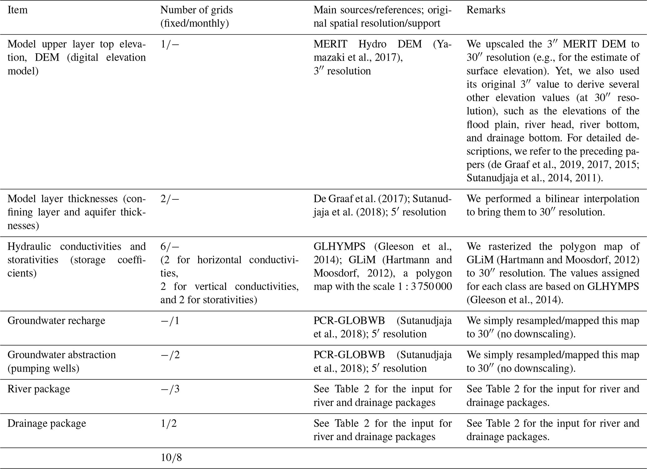
Table 2 Input data sets used for the MODFLOW river and drainage packages.

2.2.2 Runtime target in simulated years per day

As an experiment, we consider the typical “9-to-5” user to be someone who likes to start a simulation at 17:00 LT (local time) and get the results on the next working day at 09:00 LT. The target for our transient experiment for 1958–2015 is then to simulate 78 years (58 + 20 years of spin-up) in 16 h. Accordingly, this is 0.67 d, and therefore we set $R_{\mathrm{tgt}}=\mathrm{78}/\mathrm{0.67}=\mathrm{117}$ SYPD.

2.2.3 Dutch national supercomputer Snellius

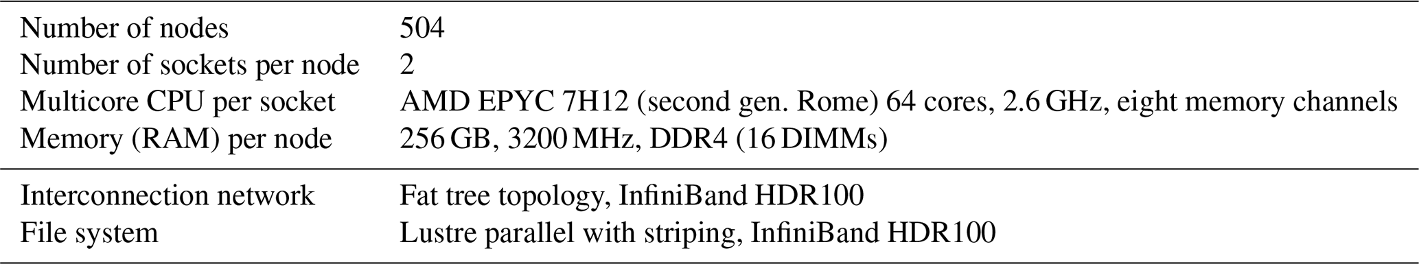
All our experiments were conducted on the Dutch national supercomputer Snellius (SURFsara, 2021), a cluster computer using multicore CPUs that are easily accessible to users from Dutch universities and Dutch research institutes. It consists of heterogeneous distributed memory nodes (servers), where we restrict to using default worker nodes having 256 GB¹ memory (“thin” nodes; see Table 3) that are tightly connected through a fast interconnection network with a low latency and high bandwidth. Each node houses two 64 core Advanced Micro Devices (AMD) CPUs that connect to 256 GB of local memory through two sockets. For this study, a storage of 50 TB and a maximum of 3.8 million files is used that is tightly connected to the nodes, enabling parallel input/output (I/O), using the Lustre parallel-distributed file system. Since the Snellius supercomputer is a (more or less) mainstream cluster built with off-the-shelf hardware components, we believe that our parallelization approach is well applicable to many other supercomputers.

Table 3 Configuration of the default computing nodes used on the Dutch national supercomputer Snellius (SURFsara, 2021).

2.3 Workflow description

2.3.1 Model workflow and node selection workflow

The main workflow for pre-processing and running the four models within GLOBGM is given by Fig. 4a. The so-called model workflow uses data that are initially generated by the process “Write Tiled Parameter Data” that writes the 30^′′ grids (see Table 1) using a tiled-based approach in an embarrassing parallel way (see Sect. 2.3.2 for more details). For the model workflow, prior to the actual partitioning and writing the model files in an embarrassing parallel way (viz. the process “Partition & Write Model Input”; see Sect. 2.3.4), a preparation step is done for the partitioning (the process “Prepare Model Partitioning”; see Sect. 2.3.3). The general idea behind this preparation step is to simplify the embarrassing parallelization for generating the submodels by storing all required mappings associated with the unstructured grids for the continents and islands, boundary conditions, areas, connectivities, and data tiling. By doing this, we do not have to recompute the mappings for each submodel and therefore save runtime. First, these mappings are used to assign the areas for the catchment partitioning, therefore requiring runtime that is negligible. Second, these mappings are used for a fast direct-access read of (tiled parameter) data required for assembling the submodels in parallel. The final step in the model workflow is to run the models on a distributed memory parallel computer (process “Run Model” in Fig. 4a).

Figure 4 (a) Model workflow for processing GLOBGM. A red box and pink box denote the embarrassing parallel and distributed memory parallel processes, respectively (see Sect. 2.1). (b) Node selection workflow using the model workflow. Workflow symbols used show the process (blue), decision (green), and manual input (orange).

It should be noted that in our workflow we have deliberately left out the post-processing used in this study. The reason for this is that we only perform limited post-processing and mainly focus on measuring the performance of the model simulation. In our post-processing, runtimes and data storage for transient evaluation are low, since we use the direct-access reading of binary output and only generate time series for a limited number of selected well locations. However, in a real-life application of GLOBGM, more output data may need to be processed, resulting in non-neglectable runtimes. In that case, post-processing could benefit from parallelization.

Figure 4b shows the node selection workflow, which uses the model workflow (Fig. 4a). The main purpose of the node selection workflow is to estimate the number of nodes $N_{\mathrm{nod}}^i$ to be used for each model i. This estimation is done by conducting a strong scaling experiment, meaning that the number of cores is being varied for a model having a fixed problem size. Input for this workflow is a selected model $\mathrm{1}\le j\le N_m$, with a convenient grid size $\left(N_{\mathrm{cell}}^j\right)$ and simulation period. Straightforward grid cell partitioning is applied (see Sect. 2.1.4), as well as a straightforward iteration scheme. Starting from $N_{\mathrm{nod}}^j=\mathrm{1}$, in each iteration of this workflow, the number of cores (or MPI processes) $N_p^j$ is chosen to be a multitude of the number of cores per node N_CPN; hence, $N_p^j=N_{\mathrm{nod}}^j\cdot N_{\mathrm{CPN}}$. Then, the model workflow generates the model input files for this number of cores, followed by running the model to obtain runtime performance R^j. The iteration finishes when R^j≥R_tgt, and the target submodel size (number of grid cells) is determined by $B_{\mathrm{tgt}}=N_{\mathrm{cell}}^j/N_p^j$. Using this submodel size, for each model $i=\mathrm{1},\mathrm{\dots },N_m$, the number of nodes is given by $N_{\mathrm{nod}}^i=⌈N_{\mathrm{cell}}^i/B_{\mathrm{tgt}}⌉$, where ⌈⋅⌉ denotes the ceiling function. Then, the number of cores to be used for each model $i=\mathrm{1},\mathrm{\dots },N_m$ follows straightforwardly from $N_p^i=N_{\mathrm{nod}}^i\cdot N_{\mathrm{CPN}}$. The (maximum) total number of nodes being used for GLOBGM we denote by $N_{\mathrm{nod}}={\sum }_i{N}_{\mathrm{nod}}^i$.

2.3.2 Model workflow: write tiled parameter data

In the offline coupling of PCR-GLOBWB to MODFLOW (see Sect. 2.2.1), all model parameter data required for the MODFLOW models are written prior to simulation. For this reason, the PCR-GLOBWB-MODFLOW Python scripts that use PCRaster Python modules (Karssenberg et al., 2010) are slightly modified for the MODFLOW module to process and write 30^′′ PCRaster raster files (uncompressed, 4 bytes, and single precision). The processing is done for a total of 163 squared raster tiles of 15^∘ with 30^′′ resolution (1800×1800 cells), enclosing the global computational grid (see Fig. 5). Using tiles has benefits for two reasons. First, using tiles cancels a significant number of redundant sea cells (missing values), thus reducing the data storage for storing one global map from 3.47 to 1.97 GB in our case (43 % reduction). Second, using tiles allows (embarrassing) parallel pre-processing to reduce runtimes. In our pre-processing, the 163 tiles are distributed proportionately over the available N_nod nodes. It should be noted that, although the tiling approach is quite effective, many coastal tiles still have redundant sea cells. Since missing values do not require pre-processing, one might argue that these tiles would result in a parallel workflow imbalance. However, the version 4.3.2 of PCRaster that we used does not treat missing values differently, and therefore, choosing tiles of equal sizes seems to be appropriate. It should also be mentioned that choosing 15^∘ tiles is arbitrary, and different tile sizes could be chosen.

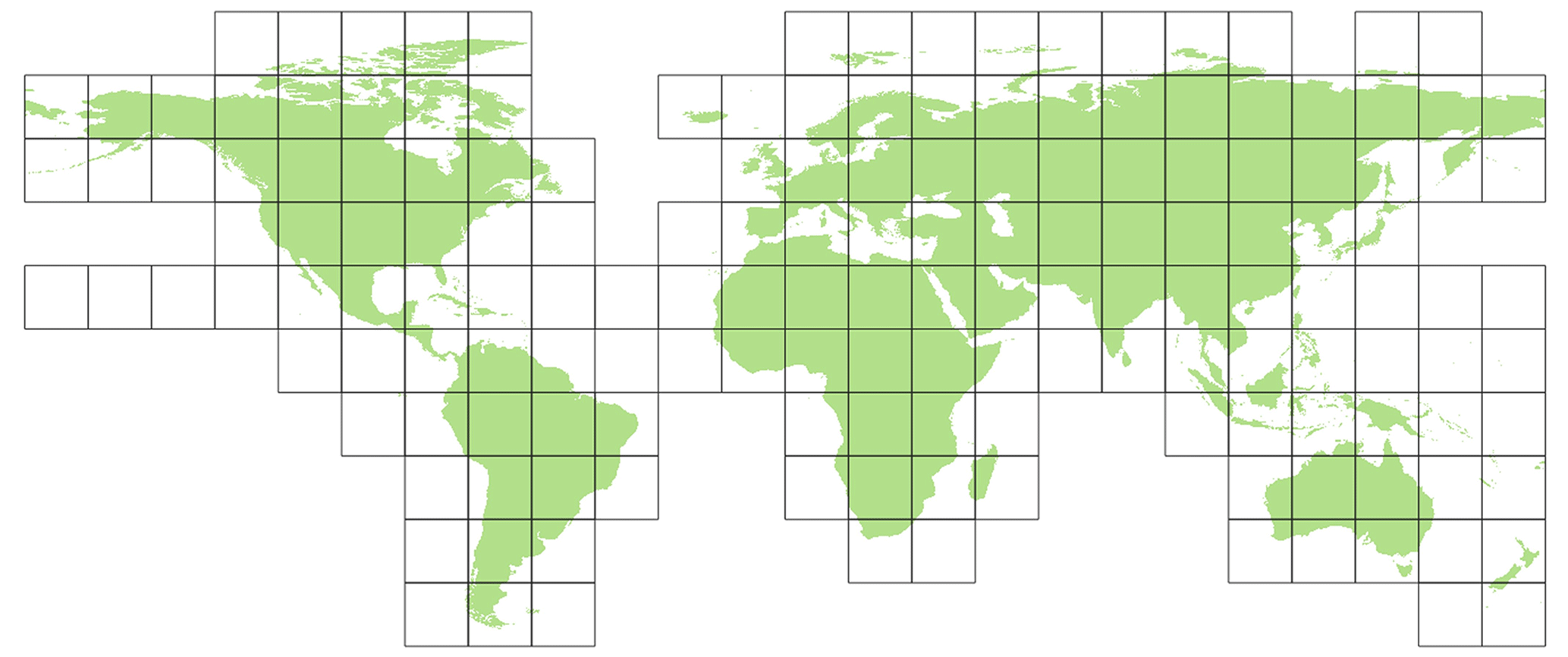
Figure 5 Parameter data tiles having 30^′′ resolution and 15^∘ size (1800×1800 cells), with a total of 163.

2.3.3 Model workflow: prepare model partitioning

The workflow for preparing the partitioning is given by Fig. 6 in more detail. This workflow derives and writes all necessary mappings that are being used for the process “Partitioning & Write Model Input” (see Sect. 2.3.4). It includes the two options for generating areas (see Sect. 2.1 and “A” and “B” in Fig. 6, respectively).

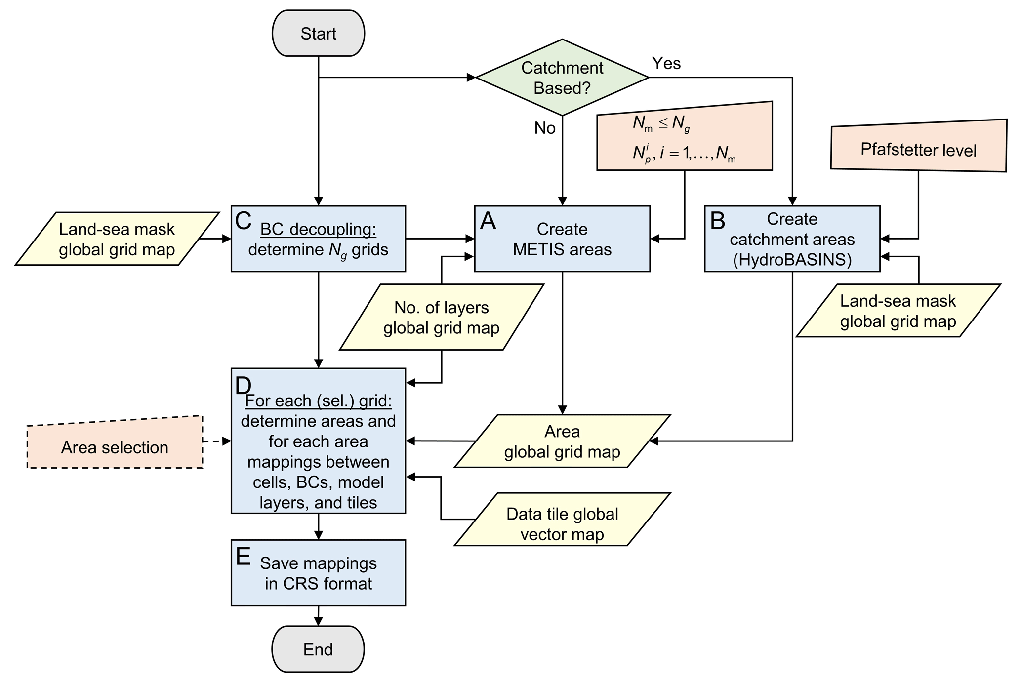
Figure 6 The process to “Prepare Model Partition” in detail, with respect to the workflow in Fig. 4a. BC is for boundary condition; CRS is for compressed row storage. Workflow symbols used show the process (blue), decision (green), manual input (orange), and input data (yellow).

When METIS areas are chosen to prepare for straightforward grid cell partitioning, areas are derived from grids g_n, $n=\mathrm{1},\mathrm{\dots },N_g$ that are disjoint and increasing in size, corresponding to continents and islands (see Sect. 2.1 and process “C” in Fig. 6). For each (continental-scale) model i, $\mathrm{1}\le i<N_m$, exactly one grid g_i is taken, and for the remainder (islands) model i=N_m, the grids g_n, $n=N_m,\mathrm{\dots },N_g$ are taken. Applying METIS partitioning for these grids to obtain $N_p^i$ partitions is then straightforward (see Sect. 2.1.4).

When catchment areas are chosen to prepare for catchment partitioning, HydroBASINS catchments are determined at the global 30^′′ extent (see process “B” in Fig. 6). This is done for a given Pfafstetter level that directly relates to the number of catchments. First, local catchment identifiers (IDs) for the HydroBASINS polygons (v1.c, including lakes) are rasterized to 30^′′ for the corresponding eight HydroBASINS regions, numbered consecutively, and merged to the global 30^′′ extent. Second, extrapolation of the catchment IDs in lateral direction near the coastal zone is done using the (extended) global 30^′′ land–sea mask and a nine-point stencil operator. Third, the nine-point stencil operator is used to identify independent catchments, and new IDs are generated and assigned where necessary.

The result of creating METIS or catchment areas is stored in a global 30^′′ map with unique area IDs. This map is the input for process “D” in Fig. 6, together with the grid definition, a (vector-based) definition of the data tiles with bounding boxes, and a global 30^′′ map with the number of model layers per cell. Optionally, areas can be selected by a user-defined bounding box, by polygon, or ID, allowing users to prepare a model for just a specific area of interest. However, in this study we limit ourselves to the global extent only, and therefore, this option is not being used. In process “D”, for each continent or island, all required mappings are determined for each of the covering areas, including the global index cells numbers and bounding box, neighboring areas and cell-to-cell interfaces, location of boundary conditions, connected data tiles, and number of model layers per cell. An undirected graph is constructed using the compressed row storage (CRS) format for efficient data storage with pointers (counters) to the (contiguous) bulk data with mappings. In process “E” in Fig. 6, these mappings are saved to binary files that allow for fast direct-access reading of all mappings required for the partitioning and writing the model input (see “Partitioning & Write Model Input”; Sect. 2.3.4).

2.3.4 Model workflow: partition and write model input

The workflow for the partitioning and writing the model input files (Fig. 7) consists of three processes: the “Area-Based Graph Partitioning” (A), “Assemble & Write Submodel Input Data” (B), and “Assemble & Write Inter-Submodel Connections” (C). This workflow is set up in a flexible way, such that it enables embarrassing parallel computing for a given range of models and submodels. This means that for selected models and submodels, data can be processed independently by using fast area-based graph partitioning and using the pre-defined and stored mappings.

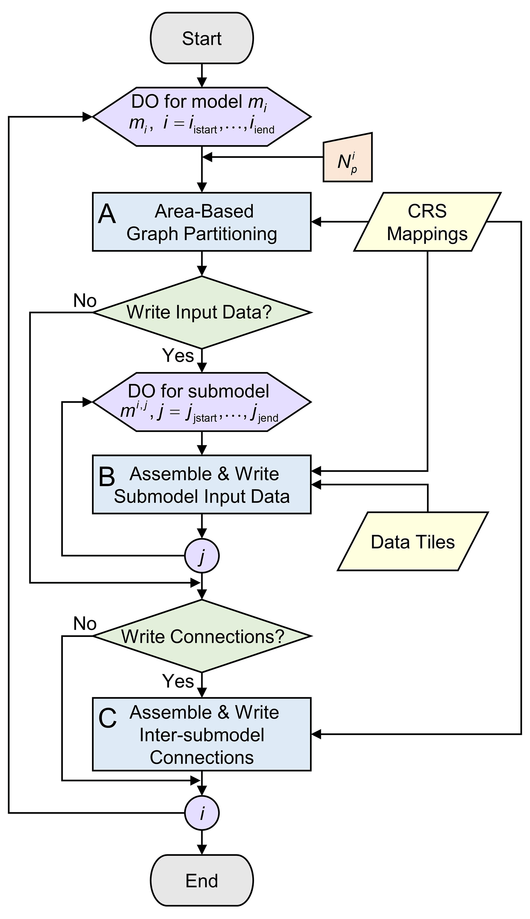
Figure 7 Process “Partition & Write Model” shown in detail with respect to the model workflow in Fig. 4a. Workflow symbols used show the process (blue), decision (green), manual input (orange), input data (yellow), and iterator (purple).

The first step is to perform the partitioning (see “A” in Fig. 7). The goal is to determine the submodel partitions by optimally assigning areas to balance the parallel workload using METIS while minimizing the edge cuts. For a model mⁱ, first, all necessary area data (cumulative vertex and edge weights and connectivities) are collected from the saved mappings that are a result of the “Prepare Model Partitioning” workflow (see Sect. 2.3.3). For each model mⁱ, $i=\mathrm{1},\mathrm{\dots },N_m-\mathrm{1}$, this is done for all areas belonging to grid g_i; for the remaining model $m^{N_m}$, this is done for all the areas belonging to grids $g_{N_m},\mathrm{\dots },g_{N_g}$. After constructing the graph for model mⁱ, METIS is being called to partition the graph into user-defined $N_p^i$ parts.

Figure 8 depicts the graphs associated with the example of Fig. 3. The vertices correspond to catchments and the edges to the connectivities between the catchments. Since, in this example, the number of disjoint grids N_g>N_m, which is generally the case, the associated graph for the (remaining) model m² is disconnected, while the graph for model m¹ is connected. The vertex weights are defined as the sum of the 30^′′ cell weights for a corresponding catchment, and the edges are defined as the sum of the shared cell faces between the catchments (see Sect. 2.1). Focusing on the vertex weights for the example graph, let Wⁱ denote the model weight of model i and w^i,j the submodel weight, such that $W^i={\sum }_j{w}^{i,j}$. In this example, model m¹ has a total weight of W¹=100 divided into two submodels, each having a weight of $w^{\mathrm{1},\mathrm{1}}=w^{\mathrm{1},\mathrm{2}}=\mathrm{50}$. Following Karypis and Kumar (1998), we here define the load imbalance for a model i as the maximum submodel weight divided by the average (target) weight; hence, $I_i=\underset{j}{max}{w}^{i,j}/(W^i/N_p^i)=N_p^i\cdot \underset{j}{max}{w}^{i,j}/W^i$. In this definition, the model is perfectly balanced when I_i=1, and load imbalance occurs when I_i>1. Assuming that Amdahl's law holds (Amdahl, 1967), it follows that the speedup (and hence parallel performance) is proportional to $I_i^{-\mathrm{1}}$. Defining the imbalance increase as $I_i^{\ast }=\mathrm{100}\cdot (I_i-\mathrm{1})$[%], then for model m¹, the submodels are perfectly balanced $(I_{\mathrm{1}}^{\ast }=\mathrm{0}$ %). On the other hand, the catchments for model m² could not be perfectly distributed over the two submodels, since the second submodel has a larger weight, $w^{\mathrm{2},\mathrm{2}}=\mathrm{21}$, than the first submodel, $w^{\mathrm{2},\mathrm{1}}=\mathrm{19}$. Therefore, the load imbalance for the second model, having a total weight W²=40, is $I_{\mathrm{2}}^{\ast }=\mathrm{5}$ %.

In general, area-based partitioning with catchments results in an insurmountable load imbalance, depending on several factors. The amount of load imbalance depends on the (multi-level) partitioning algorithm being used, the number of catchments related to the number of partitions, the catchment geometry, and the effect that all of this has on the search space. In this study, we do not try to make any quantitative or qualitative statements on this issue. Moreover, we aim for the practical aspects for a given commonly used graph partitioner with default settings applied to a realistic set of catchments. It should be noted, as already highlighted in Sect. 2.1, that load imbalance for METIS areas can be considered to be optimal, since the number of vertices (equal to the number of lateral cells) is very large compared to the number of partitions and do not vary strongly in weight. It is verified that the obtained load imbalance never exceeds the specified maximum tolerance of I_i=1.0001.

The second step of the workflow in Fig. 7 (see “B”) is to process all submodel data. First, the resulting METIS or catchment areas assigned by METIS (the result of process “A”) are used to assemble the unstructured grid. Then, using the tiled parameter data and the CRS mappings, both the steady-state and transient model input data are written. To significantly reduce the number of model input files for a transient simulation, each submodel has exactly one binary file for storing all necessary bulk data. This is a new functionality of our MODFLOW 6 prototype. For the third and last step in the workflow of Fig. 7 (process “C”), first an inter-submodel graph is assembled for each model by the merging the inter-area graph from the CRS mappings and the derived partitions from process “A”. Second, the submodel connections (MODFLOW exchanges) are written to files, as well as wrappers for running the steady-state model, the transient spin-up model, and the actual transient model.

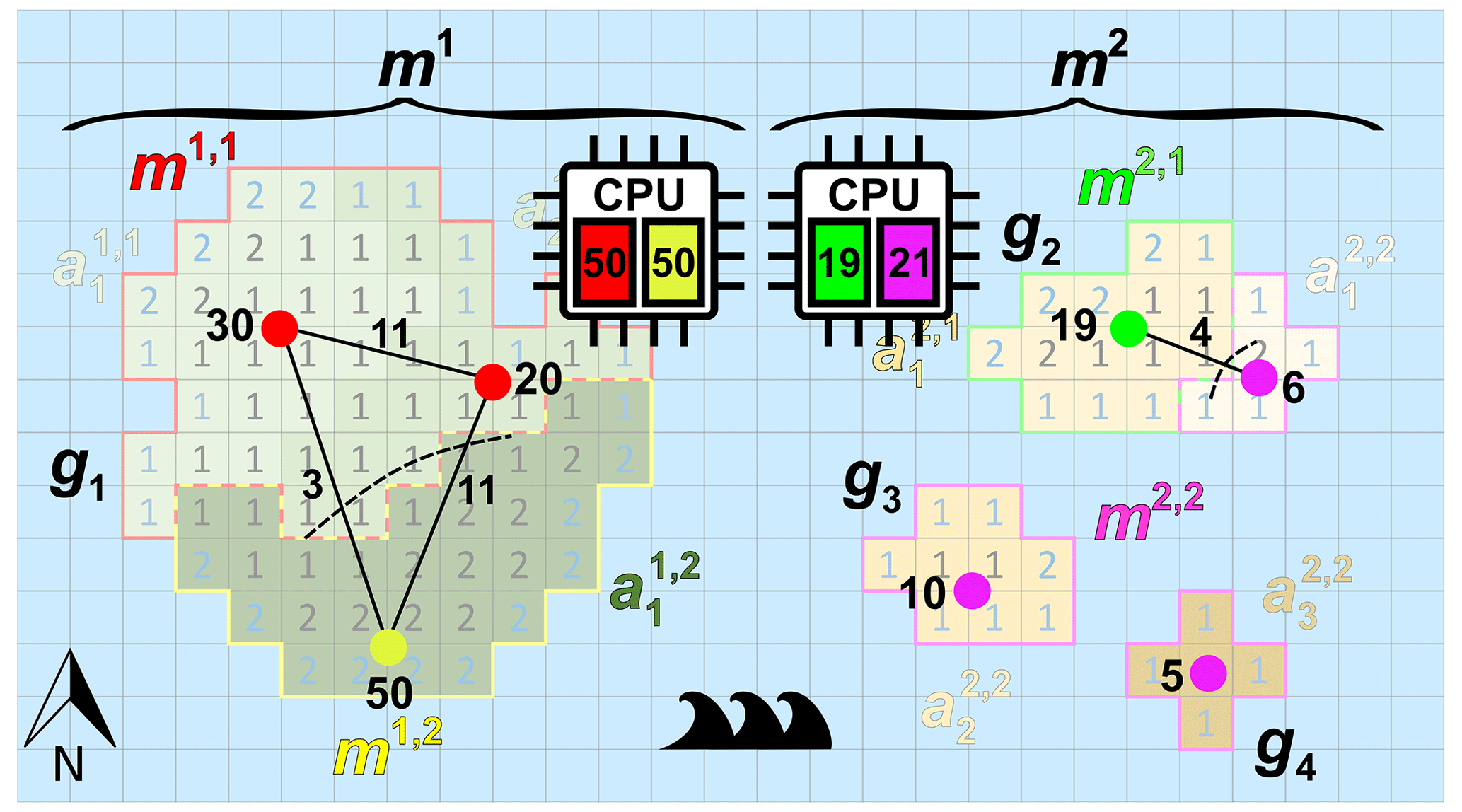
Figure 8 Example of area-based graph partitioning corresponding to the example of Fig. 3, where the work for each submodel is uniquely assigned to a core of a dual-core CPU.

2.4 A limited first evaluation of GLOBGM

Here, GLOBGM is evaluated for the CONUS for which many head measurement data sets are publicly available. For our study, we restrict to selected head observations from the United States Geological Survey (USGS) National Water Information System (NWIS) database (USGS, 2021a). For the global evaluation, where transient head time series are limited, we evaluated groundwater level fluctuations with total water storage anomalies derived from the GRACE and GRACE-FO satellites (Wiese, 2015; Wiese et al., 2016). This evaluation is limited, however, since GLOBGM v1.0 is an initial model. This means various other aspects are left for further research, namely improving model schematization (e.g., geology), improving model parameters by adding more (regional scale) data and calibration, and adding more global data sets for comparison. Our evaluation is mainly in comparison to the 5^′ PCR-GLOBWB-MODFLOW model (GGM) for which we used consistent upscaled data.

2.4.1 Steady-state hydraulic heads for the CONUS

The steady-state (i.e., long-term average) evaluation is limited to the so-called natural condition, meaning that human intervention by groundwater pumping is excluded from the model. Besides comparing GLOBGM to the GGM (of de Graaf et al., 2017), we compare the computed steady-state hydraulic heads to two other models, namely the global-scale inverse model (GIM) from Fan et al. (2017), with 30^′′ resolution and used for estimating steady-state root-water-uptake depth based on observed productivity and atmosphere by inverse modeling, and the CONUS groundwater model (CGM) from Zell and Sanford (2020), a continental-scale MODFLOW 6 groundwater model developed by the USGS for simulating the steady-state surficial groundwater system for the CONUS. Henceforth, these latter models are referred to as GIM and CGM, respectively. It should be noted that contrary to GLOBGM and the GGM, the GIM and the CGM have been calibrated on head observations. For the steady-state evaluation, we use the same NWIS wells as selected by Zell and Sanford (2020) to evaluate the performance of the four models. Mean hydraulic head residuals are computed for HUC4 surface water boundaries from the USGS Watershed Boundary Dataset (U.S. Geological Survey, 2021b) to get a spatially weighted distribution of the residuals for the CONUS.

2.4.2 Transient hydraulic heads for the CONUS

For the simulation period 1958–2015, GLOBGM computed hydraulic heads at a monthly time step are compared to NWIS time series, considering the non-natural condition (including groundwater pumping). We perform the same evaluation for a recent GGM run (de Graaf et al., 2017) and compare the outcome with GLOBGM to evaluate a possible improvement. Closely following the methodology as chosen in de Graaf et al. (2017) and Sutanudjaja et al. (2011), we compute the following long-term-averaged statistics: the sample correlation coefficient r_mo is used for quantifying the timing error between model (“m”) and observation (“o”). Furthermore, the absolute and relative interquartile range error, ${\mathrm{IQRE}}_{\mathrm{mo}}=\mathrm{|}{\mathrm{IQR}}_{\mathrm{m}}-{\mathrm{IQR}}_{\mathrm{o}}\mathrm{|}/{\mathrm{IQR}}_{\mathrm{o}}$, with IQR_m and IQR_o interquartile ranges for the model and observations, respectively, is used to quantify the amplitude error. Additionally, the trend of the (monthly averaged) time series is computed, considering the slope β_y of yearly averaged hydraulic heads from a simple linear regression with time. We assume that a time series has a trend if |β_y|>0.05 m yr⁻¹ and no trend otherwise. Transient evaluation using measurements from the NWIS database requires filtering out incomplete time series and data locations for areas that are not represented by GLOBGM. Similar to de Graaf et al. (2017), time series are selected to have a record covering at least 5 years and to include seasonal variation. However, different from de Graaf et al. (2017), we only consider well locations for sedimentary basins (including karst). Furthermore, we aggregate the computed statistics (timing, amplitude, and trend) to the same HUC4 surface water boundaries as used for the steady-state evaluation (see Sect. 2.4.1) for obtaining results at a scale that is commensurate with a global-scale groundwater model. In this way, we find HUC4s to have fewer than five NWIS wells not spatially representative, and for these HUC4s, we exclude the corresponding wells from the presented statistics. In total, the filtering resulted in 12 342 site locations selected for comparison between simulated and observed head time series (see also the Supplement).

2.4.3 Total water storage anomalies for the world's major aquifers

For the transient evaluation, we also computed the simulated total water storage (TWS) and compared it to the one estimated from GRACE gravity anomalies. For the simulated TWS, we used computed hydraulic heads from GLOBGM (multiplied by the storage coefficient) and data (for snow, interception, surface water, and soil moisture) from the PCR-GLOBWB run of Sutanudjaja et al. (2018). Here we compared the monthly simulated TWS to the monthly gravity solutions from GRACE and GRACE-FO, as determined from the JPL RL06.1Mv03CRI (Wiese, 2015; Wiese et al., 2016). For this evaluation, cross-correlations between simulated and observed TWS anomalies at the monthly and annual timescale are considered for the period of 2003–2015, with the focus on the world's major aquifers (Margat and der Gun, 2013). Monthly correlations represent how well seasonality is captured, while annual correlations measure the reproductions of secular trends as a result of interannual climate variability and groundwater depletion. It is important to note that TWS anomalies are not groundwater storage anomalies. However, interannual variation in the TWS is heavily influenced by storage changes in the groundwater system (e.g., Scanlon et al., 2021).

3 Results and discussion

3.1 Pre-processing for transient simulation

3.1.1 Node selection procedure

Figure 9a shows the performance for a HPCG strong scaling experiment (see Sect. 2.1) on a single thin node of the Dutch national supercomputer Snellius (see Table 3), up to a maximum of 128 cores using two CPUs. In this figure, the ideal performance (dashed line) is a straightforward extrapolation of the serial performance. It can be observed that a flattening occurs, starting from 32 cores, where the competition of cores for the memory bandwidth results in saturation. From this, the maximum number of cores per node is chosen as N_CPN=32 for the remainder of the experiments. For the node selection procedure (see Sect. 3.1; Fig. 4b), the Americas model is chosen (j=2), considering a 1-year simulation for 1958. This model corresponds to a “medium-sized” model consisting of $N_{\mathrm{cell}}^{\mathrm{2}}=\mathrm{77}$ million cells. Starting with $N_{\mathrm{nod}}^{\mathrm{2}}=\mathrm{1}$ node, hence using a total of $N_p^{\mathrm{2}}=\mathrm{1}\cdot \mathrm{32}=\mathrm{32}$ processor cores, Fig. 9b shows that for the third iteration the measured performance exceeds the target performance, $R^{\mathrm{2}}=\mathrm{145}>\mathrm{117}=R_{\mathrm{tgt}}$; hence, $N_{\mathrm{nod}}^{\mathrm{2}}=\mathrm{3}$ nodes for a total of $N_p^{\mathrm{2}}=\mathrm{3}\cdot \mathrm{32}=\mathrm{96}$ cores. Therefore, the target submodel size is $B_{\mathrm{tgt}}=N_{\mathrm{cell}}^{\mathrm{2}}/N_p^{\mathrm{2}}=\mathrm{77}/\mathrm{96}=\mathrm{0.8}$ million 30^′′ cells. Then, by computing $N_{\mathrm{nod}}^i=⌈N_{\mathrm{cell}}^i/B_{\mathrm{tgt}}⌉$ for $i=\mathrm{1},\mathrm{\dots },\mathrm{4}$ and calculating back the number of nodes and cores, the Afro–Eurasia model is estimated to use seven nodes and 224 cores to meet the target performance, the Americas model three nodes and 96 cores, and the Australia and Islands models each use a single node and 32 cores (see Table 4). Hence, the total maximum number of nodes in the study for GLOBGM is N_nod=12 for a total of 384 cores. This results in an average submodel size of 0.72 million 30^′′ cells.

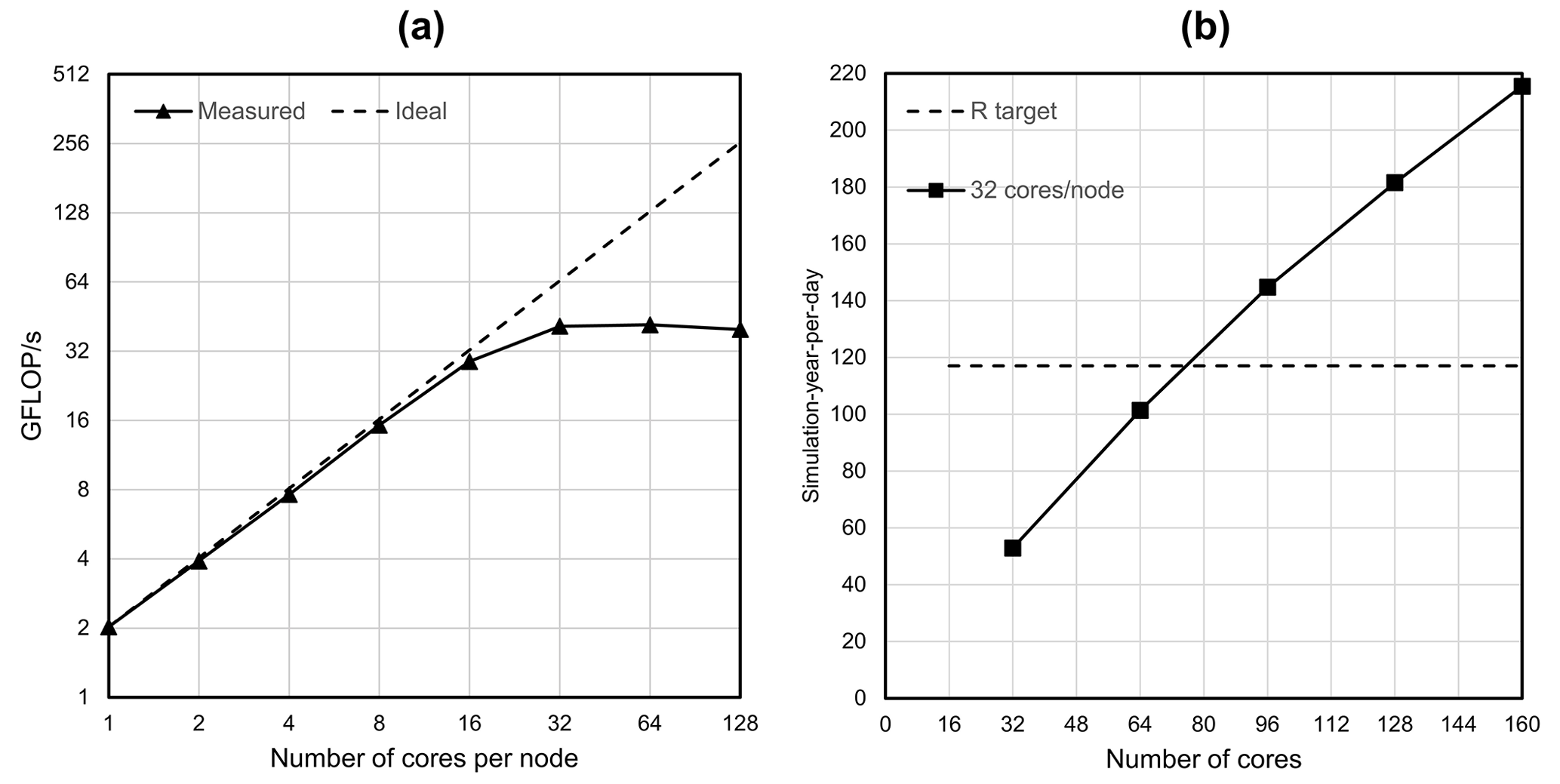
Figure 9 (a) HPCG performance results in GFLOPS for a model having 104³ cells and a maximum runtime of 60 s. (b) Performance estimation for the Americas model considering a transient simulation for 1958.

Table 4 Configuration of nodes and cores resulting from the node selection procedure.

3.1.2 Tiled parameters and model input

The parameter pre-processing for the 163 data tiles (see Sect. 2.3.2) is distributed over the 12 available nodes, such that the first 11 nodes do the pre-processing for 14 tiles each and the last node for 9 tiles. For each tile, the average runtime for pre-processing 1958–2015 (696 stress periods) is 3:25 h. In serial, this would require 558.7 core hours in total or ∼ 23 d of runtime accordingly. This results in 5578 PCRaster files ($\mathrm{10}+\mathrm{696}\cdot \mathrm{8}=\mathrm{5578}$; see Table 1) for each tile, requiring 68 GB of storage. Hence, in total, 909 214 files are written in parallel, amounting to 10.8 TB storage. Using data tiles therefore saves storing ∼ 8 TB of redundant data (43 % reduction; see Sect. 2.3.2).

Table 5 shows the pre-processing runtimes for each submodel to generate the transient MODFLOW input data in parallel using the node configuration as in Table 4, considering straightforward grid cell partitioning (see Sect. 2.1). On average, it takes up to half an hour to do the pre-processing for each model (Afro–Eurasia, the Americas, and Australia). As can be observed, clearly not all submodels require the same runtime, and there is a spread in distribution. Looking at the standard deviation (SD in Table 5), this is significantly large for the Islands model, measuring about 2.5 h. We believe that this is inherent to our chosen partitioning for the Islands model, allowing submodels to have grid cells of many scattered islands that are scattered across the world (see, e.g., Fig. 10 for the slowest submodel). In this way, it is likely that random data access of scattered unstructured grid cells to the tiled parameter grids occurs, slowing down the data reading after the submodel assembly. Although pre-processing is not a focus in this study, we might improve this in the future by incorporating a clustering constraint in the partitioning strategy. For the Afro–Eurasia, Americas and Australia models, the SD is comparably small, varying from 3 to 9 min. For the total parallel pre-processing to generate model input, a total of 222 core hours was required (or ∼ 9 d of serial runtime, accordingly).

Table 5 Pre-processing runtimes for process “Assemble & Write Submodel Input Data” (see “B” in Fig. 7). SD is for standard deviation.

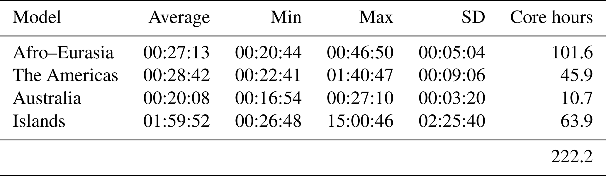
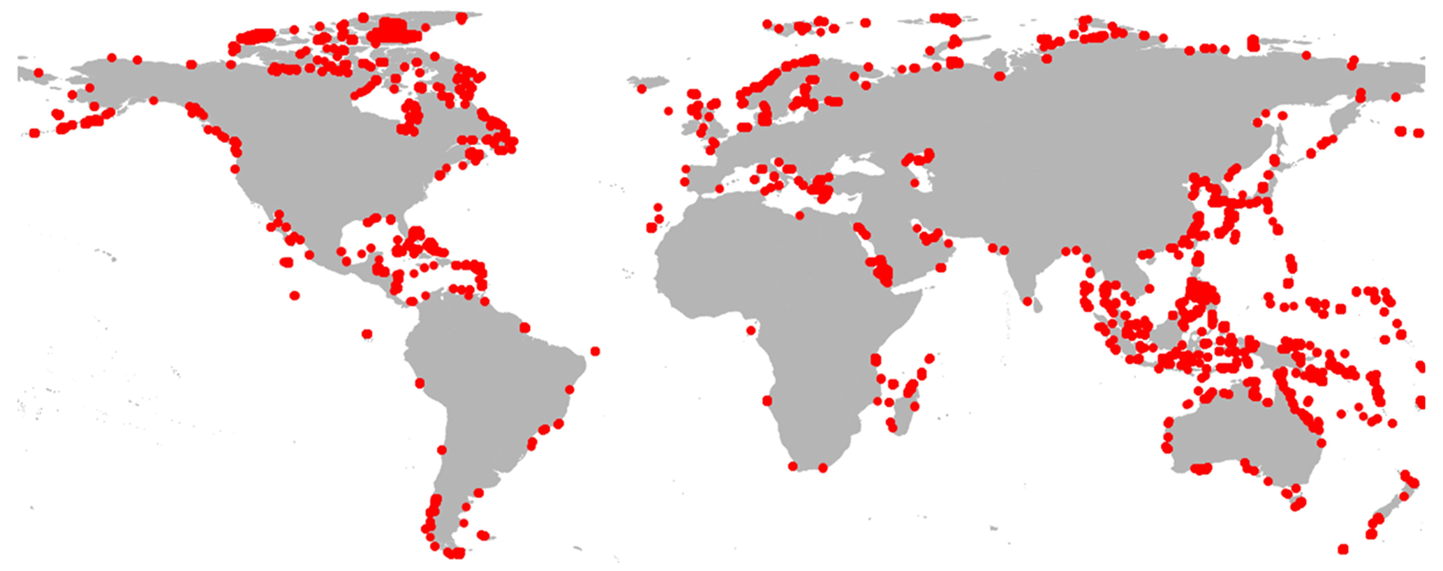
Figure 10 Location of unstructured grid cells (red) for a submodel of the Islands model, showing scattering and requiring large pre-processing runtime for writing the submodel input data.

3.2 Parallel performance for transient simulation

Figure 11 shows the main parallel performance results for GLOBGM, considering simulation of 1958–2015, including a 20-year spin-up using the node/core configuration (as in Table 4), and applying straightforward grid cell partitioning (see Sect. 2.1.4). This figure shows that the target performance of 117 SYPD (16 h of runtime) was achieved for all models (green bars), showing a significant increase in performance compared to the serial case (red bars). For the largest Afro–Eurasia model, the serial runtime could be reduced significantly from ∼ 87 d (0.9 SYPD) to 0.63 d (or ∼ 15 h; 123.6 SYPD) when using 224 cores. This corresponds to a speedup factor of 138.3, with a parallel efficiency of 62 %. In general, for all four models, the parallel efficiency is ∼ 60 %. Note that Fig. 11 also shows the metric of core hours per simulated year (CHPSY) on the right vertical axis that is defined as the cumulative runtime over all processor cores being used for simulation a single year. With CHPSY, the actual parallel runtime can be easily obtained by multiplying CHPSY with the number of simulated years and consecutively dividing by the number of processor cores being used. It should be noted that the serial performance was only evaluated for a single year, i.e., 1958. The reason for this is that serial runtime for the entire simulation period was too long (e.g., ∼ 27 CHPSY for Afro–Eurasia; hence $\mathrm{27}\cdot \mathrm{78}=\mathrm{2106}$ h or 87 d runtime), and it would exceed the maximum allowed runtime of 5 d on a single Snellius node. For each parallel run, however, the performance is evaluated for 78 years (20 times 1958 + 1958–2015). Furthermore, in our experiments, each serial/parallel run is only evaluated twice, taking the average performance values for two runs only. We therefore did not account for any statistic (hardware related) runtime variation on the Snellius supercomputer. The reason for this was the limited total number of available core hours, where one full GLOBGM run requires ∼ 24 000 core hours.

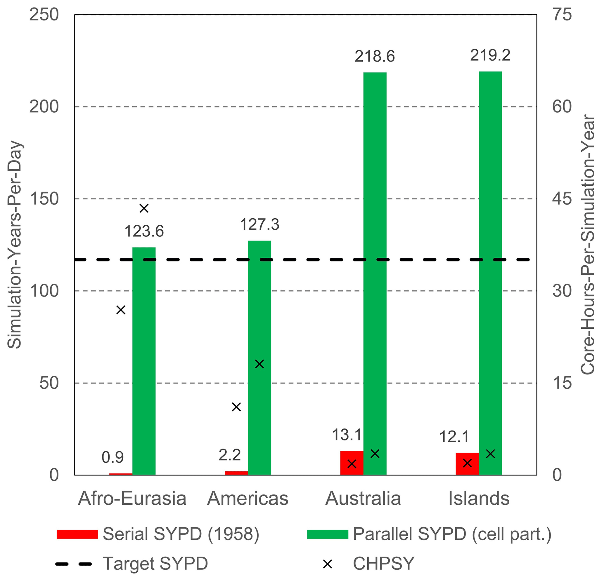
Figure 11 Parallel performance results for the models of GLOBGM, considering straightforward grid cell partitioning (“cell part.”). Left vertical axis shows the simulated years per day (SYPD; bars), and the right vertical axis shows the core hours per simulated year (CHPSY; crosses). Serial performance is computed for 1958 only.

Figure 11 shows that there is a performance difference between the models. The slowest model is the Afro–Eurasia model, followed by the Americas model, the Australia model, and Islands model. This holds for both the serial and for the parallel case. For the serial performance, it is obvious that the main difference in performance is caused by the difference in model sizes. The serial performance difference between the largest Afro–Eurasia model with 168 million cells and the smallest Australia model with 16 million cells that is 10 times smaller can be directly related to fewer FLOPS and less I/O.

However, also the difference in total number of iterations (linear plus non-linear) contributes to this; considering 1958, the serial Afro–Eurasia model required 1.47 times more iterations to converge than the Australia model. The difference in iterations is likely related to the problem size and the number of the Dirichlet boundary conditions affecting the matrix stiffness. For the parallel case, this effect is enhanced, since the parallel linear solver has different convergence behavior and generally requires more iterations to converge when using more submodels, which is inherent to applying the additive Schwarz preconditioner. In general, for the parallel performance considering straightforward grid cell partitioning, the increase in the total number of iterations is in the range of 34 % to 58 %. That directly relates to a significant performance loss. Although we found that the parallel performance is adequate to reach our performance goal, reducing the total number of iterations is therefore something to consider for further research. We might improve the number of iterations by tuning the solver settings or applying a more sophisticated paralleled preconditioner. However, in general, users do not spend time on tuning solvers settings, and we therefore take them as they are. Furthermore, as a first attempt to reduce iterations, we did not see any improvement by using the additive coarse-grid-correction preconditioner.

Moreover, the difference in parallel performance could be explained by the differences in submodel (block) sizes (see Table 4). Due to rounding the number of cores to the number of cores per node, the block sizes for the Australia and Islands models are ∼ 1.5 smaller than the block sizes for the Afro–Eurasia and Americas models, which directly results in an increasing performance.

Besides the increase in iterations, memory contention contributes to the loss of parallel performance (see Sect. 2.1.5), even when using 32 cores per node out of 128 cores. From the HPCG test (see Fig. 9a), the parallel efficiency using 32 cores per node is 63 %, which is likely to be a representative value for the MODFLOW linear solver. For MODFLOW, however, this value is likely to be slightly larger because of non-memory bandwidth-dependent components. Comparing to a 1958 run for the Americas model, and using one core per node, we estimate the maximum efficiency to be 77 %. Extrapolating this to the Afro–Eurasia model, this means that ∼ 172 cores could be used efficiently, increasing the efficiency to 80 %. This value is more in range with what we expect from preceding research using MODFLOW (Verkaik et al., 2021b).

In Fig. 12a, the performance results are given for catchment partitioning considering HydroBASINS Pfafstetter levels 8, 6, and 5 (see Sect. 2.1), which are chosen for illustration. Level 7 was excluded deliberately in the search for finding a significant performance decrease and minimizing the allocated budgets on the Snellius supercomputer. In general, for the Australia and Islands models, the target performance is exceeded for all HydroBASINS levels. For the Afro–Eurasia and Americas models, level 8 is sufficient to reach the target, and level 6 results in performance slightly below the target. For these models, level 5 results in about three-quarters of the target performance. In general, using HydroBASINS catchments up to Pfafstetter level 6 seems to give adequate results. Except for the Australia model, performance decreases when the Pfafstetter level decreases. The reason why this does not apply to the Australia model is because of the slight iteration increase for level 8. In Fig. 12b, the performance for catchment partitioning (Fig. 12a) is normalized, with the performance using straightforward grid cell partitioning (Fig. 11) and the associated total iteration count. Clearly, the performance slope is correlated to the inverse of the load imbalance determined by METIS (see Sect. 2.3.4). Since many factors may contribute to the load imbalance, like the specific multilevel heuristics being used, specified solver settings, characteristics of the graph subject to partitioning, and limitations of the specific software library, an in-depth analysis is beyond the scope of this study. Here, we simply assume that this imbalance is a direct result of the coarsening associated with decreasing Pfafstetter levels for a fixed number of submodels, reducing the METIS graph-partitioning search space.

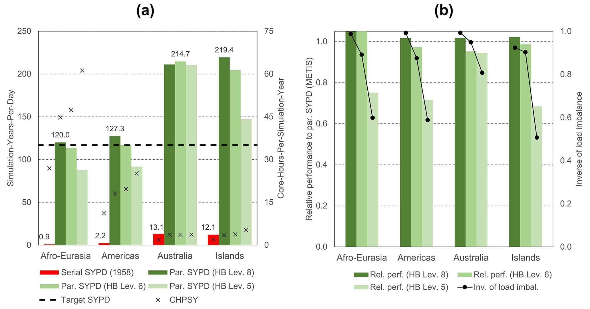
Figure 12 (a) Performance results for GLOBGM, considering catchment partitioning using the HydroBASINS (HB) catchment areas for Pfafstetter levels 8, 6, and 5. The left vertical axis shows the SYPD (bars); the right vertical axis shows the CHPSY (crosses). Serial performance is computed for 1958 only. (b) Relative performance to using straightforward grid cell partitioning, normalized with the corresponding total number of iterations (bars), and the inverse of the METIS load imbalance I_i (lines).

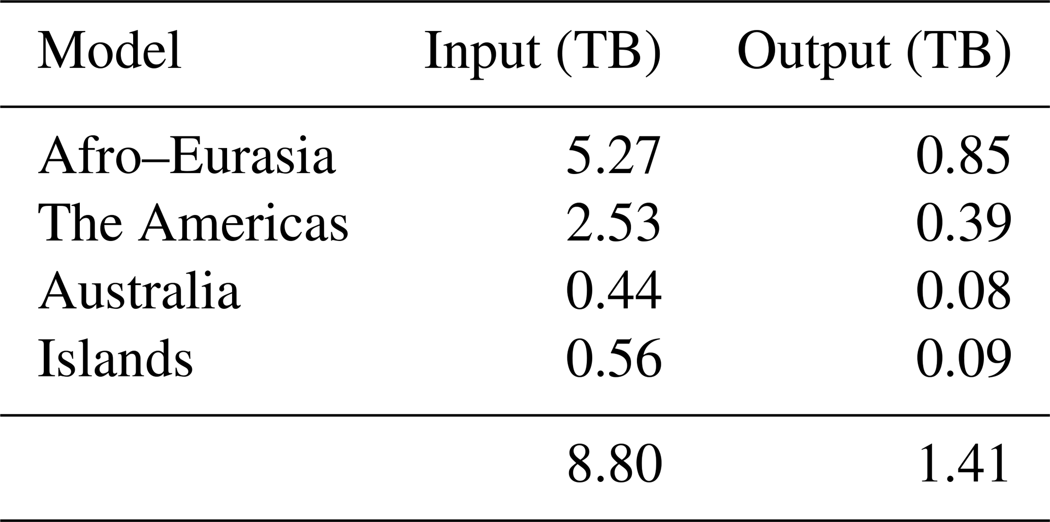
The required storage for each run is given by Table 6, where monthly computed hydraulic heads were saved exclusively during simulation. For this, one transient global run required 8.8 TB of input and 1.4 TB of output.

Table 6 Input and output of GLOBGM for simulating the period 1958–2015.

3.3 A limited first evaluation of GLOBGM

3.3.1 Steady-state hydraulic heads for the CONUS

Figure 13 shows the steady-state water table depth residuals aggregated to the HUC4 surface watershed boundaries for the CONUS, comparing GLOBGM to the GGM (de Graaf et al., 2017), the GIM (Fan et al., 2017), and the CGM (Zell and Sanford, 2020; see Sect. 2.4.1). For Fig. 13, all NWIS measurements from Zell and Sanford (2020) are considered for both sedimentary basins and mountain ranges. In addition to Fig. 13b, in Fig. A1 in Appendix A, the results for GLOBGM and the GGM are shown for sedimentary basins with and without karst, showing the best results for sedimentary basins excluding karst, as is to be expected from the presumed application range (see Sect. 2.2.1).

Clearly, GLOBGM is an improvement compared to the GGM, where the frequency distribution of the GGM residuals (red line in Fig. 13b) shifts towards the residuals of GLOBGM (green line in Fig. 13b). Hence, refining from 5^′ to 30^′′ resolution is resulting in higher and more accurate hydraulic heads. A likely explanation for this better performance is that GLOBGM, having a higher resolution, is better at following topography and relief, in particular for resolving smaller higher-altitude groundwater bodies in mountain valleys. Also, higher-resolution models have a smaller-scale gap with the in situ head observations in wells. However, the GIM and CGM seem to give a better performance than GLOBGM. A reason for this could be that those models are calibrated, using many data from the Unites States, while GLOBGM (and the GGM) is not. In general, the computed hydraulic heads with GLOBGM still seem rather low. Analyzing the possible causes for this is left for further research.

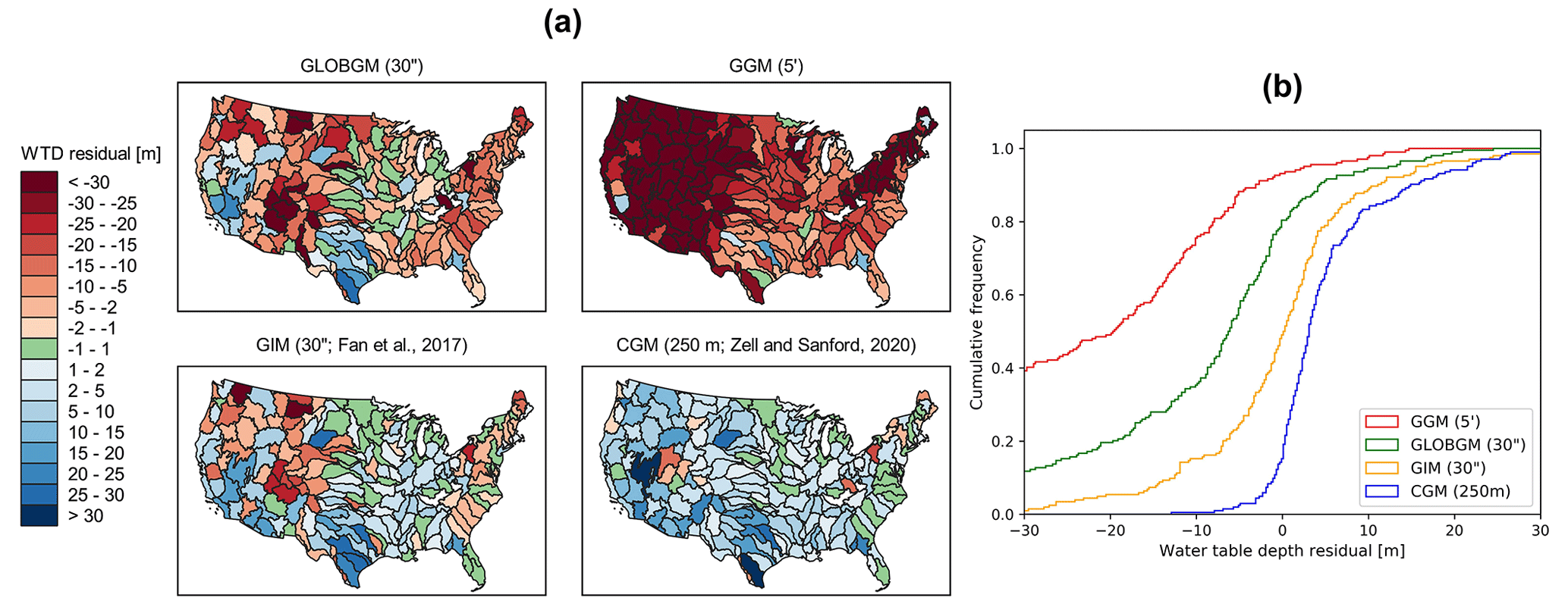
Figure 13 (a) Water table depth (WTD) residuals aggregated to HUC4 units for steady-state GLOBGM compared to the GGM, the GIM model of Fan et al. (2017) and the CGM of Zell and Sanford (2020). (b) Corresponding cumulative frequencies.

3.3.2 Transient hydraulic heads for the CONUS

Figure 14 shows the results for the transient evaluation of GLOBGM, comparing the computed transient hydraulic heads for 1958–2015 to the transient NWIS head observations. Three statistical measures are evaluated, namely the average timing (r_mo), average amplitude error (IQRE_mo), and trend classification (using β_y) (see Sect. 2.4.2). Furthermore, similar statistics are computed and added to this figure for the coarser 5^′ GGM, showing the effect of increased resolution with GLOBGM. In general, we see that GLOBGM and the GGM give very comparable results that could be further improved. For the average amplitude error, GLOBGM seems to perform slightly worse, and we do not have a straightforward explanation for this. However, GLOBGM seems slightly better with regard to trend direction and lacking a model trend. Furthermore, it can be seen that about 40 %–50 % of the (majority of the) observations have a mismatch in trend. This can likely be related to incorrect well locations and pumping rates in the model that are inherent to the applied parameterization and concepts within PCR-GLOBWB (see Table 1). This might also have effect on the discrepancies for the timing and amplitude errors and is therefore a subject for further research.

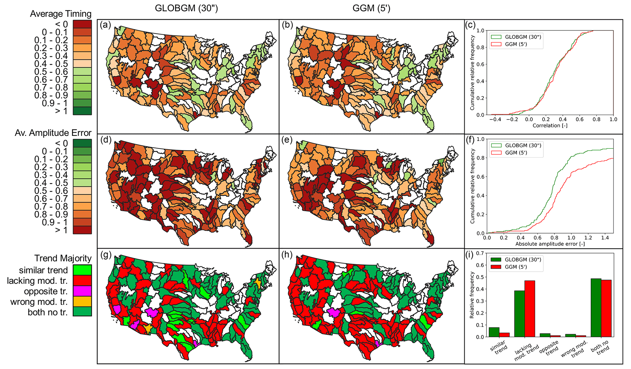
Figure 14 Evaluation of computed hydraulic heads for 1958–2015 to NWIS head observations, with the average timing (a, b, c), amplitude error (d, e, f), and trend (g, h, i) for both GLOBGM and the GGM. Plotted white colors for HUC4 units mean that fewer than five samples were found and hence were not considered representative.

3.3.3 Total water storage anomalies for the world's major aquifers

In Fig. 15 we present the cross-correlations between GRACE total water storage (TWS) anomalies at monthly and annual timescales with simulated TWS anomalies calculated from the sum of the GLOBGM (groundwater component) and PCR-GLOBWB models (Sutanudjaja et al., 2018) (other components). These results demonstrate a good overall agreement between our simulated TWS and GRACE, especially at the monthly resolution (Fig. 15a). At the annual resolution (Fig. 15b), the agreement remains satisfactory, particularly for major aquifers known for having groundwater depletion issues, such as the Central Valley, High Plains Aquifer, Middle East, Nubian Sandstone Aquifer System, and North China Plain. However, somewhat lower annual correlations are observed for the Indo–Gangetic Plain, which could be attributed to factors such as glacier storage changes that the PCR-GLOBWB model does not accurately simulate. Furthermore, the low annual correlations observed in the Amazon may be attributed to the large water storages in floodplains that remain during streamflow recession, which is not properly simulated in the used version of the PCR-GLOBWB model. Also, disagreement in South America and Africa can be attributed to the PCR-GLOBWB forcing data issues in such regions with limited availability of meteorological observations. Additionally, it is important to consider that GRACE measurements may display a higher noise-to-signal ratio in arid regions like the Sahara, especially when there are minimal storage changes or low groundwater utilization, which could contribute to relatively lower correlations in those areas.

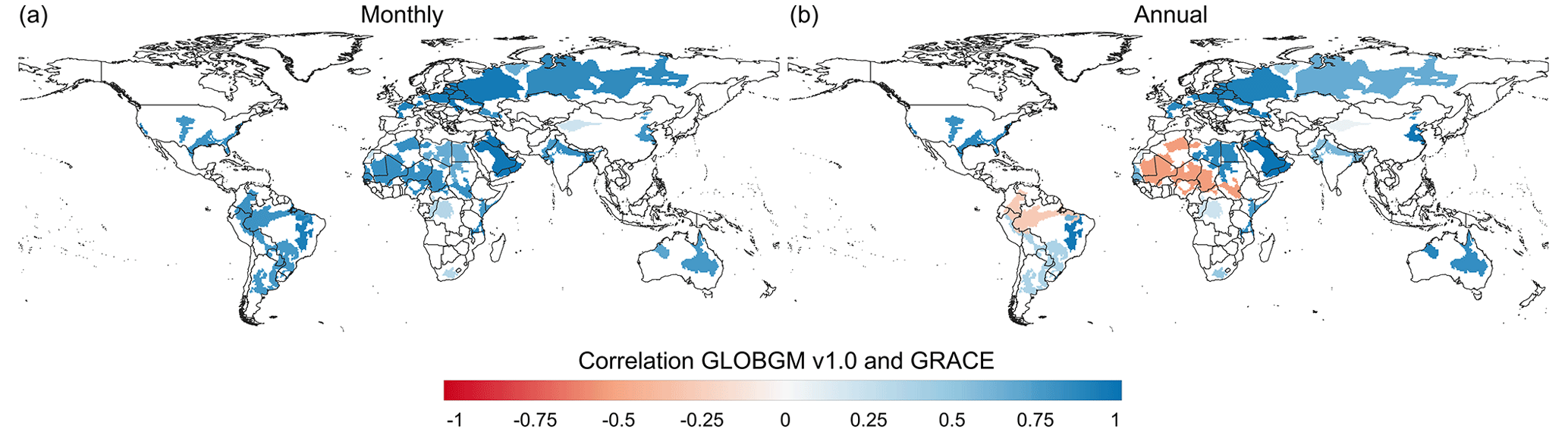
Figure 15 Correlation between monthly (a) and annual (b) TWS time series from GRACE and the ones computed from the GLOBGM (groundwater) and the PCR-GLOBWB models (snow, interception, soil moisture, and surface water). Here, we focus on the major aquifers.

3.4 Example of global-scale results

To provide an impression about the level of detail reached when simulating hydraulic heads at 30^′′ spatial resolution, steady-state and transient global map results are shown in Fig. 16. For sake of the application domain of GLOBGM (see Sect. 2.2.1), we mask out the karst areas (WHYMAP WoKAM; Chen et al., 2017). In Fig. 16a, the steady-state solution of water table depths is shown: the zoomed-in insets show the intricate details present, which are mostly guided by surface elevation and the presence of rivers. In Fig. A2 in Appendix A, cell locations are plotted where steady-state GLOBGM has a vertical flow in an upward direction to the land surface (groundwater seepage). This figure mainly shows clustering near river locations but also areas where heads underlying the confining layers exhibit an overpressure compared to the overlying phreatic groundwater. Figure 16b and c show examples of transient global map results for the GRACE period of 2003–2015, here focusing on sedimentary basins only. Figure 16b shows the hydraulic head amplitude, as represented by the interquartile range, where the amplitude size reflects the amplitude of groundwater recharge and the hydrogeological parameters (storage coefficient and hydraulic conductivity). Figure 16c shows the trends of yearly average hydraulic heads for sedimentary basins. For the areas with confining layers, the trend in the heads of the lower model cells is taken. Here, the well-known areas of groundwater depletion (Wada et al., 2010; de Graaf et al., 2017) are apparent. However, areas with spurious trends can also be seen that may be connected to incomplete model spin-up. Furthermore, positive trends can be seen, which may be connected to increased precipitation related to climate change. In the Supplement, we provide two animations for computed water table depths, with one for monthly values and another one for yearly averaged values. To show the dynamic behavior of the hydraulic heads, we show these results relative to the heads of 1958.

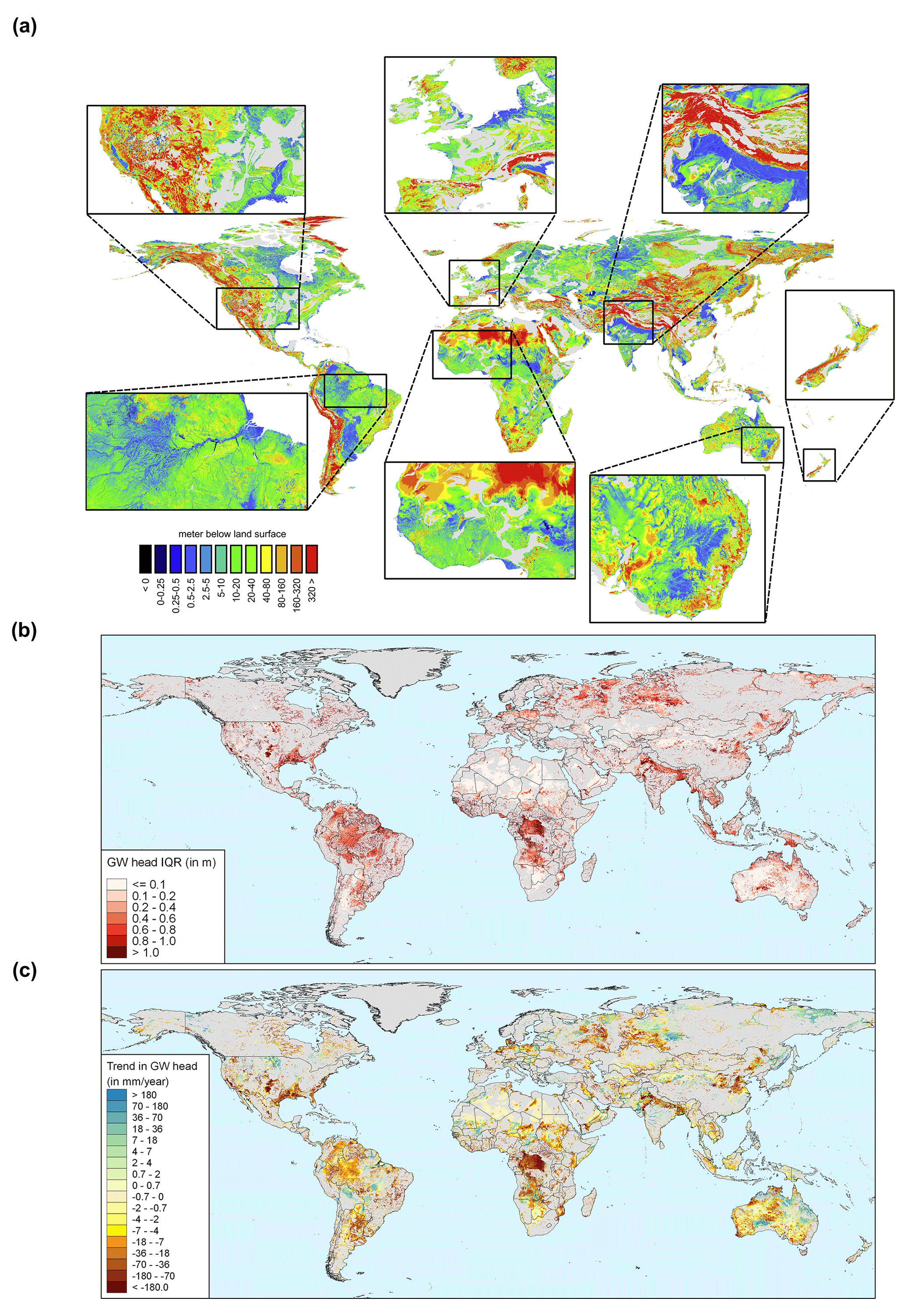
Figure 16 Example outputs of GLOBGM. (a) Steady-state water table depth with detailed zoomed-in insets. (b) Water table amplitude for 2003–2015, as represented by the interquartile range (IQR). (c) Hydraulic head trends for 2003–2015 for the aquifer (lower model layer). In all panels, a mask is applied for karst areas; in the lower panels of (b) and (c), an additional mask is applied for mountain ranges.

4 Conclusions and recommendations

The PCR-GLOBWB-MODFLOW global-scale groundwater model at 30^′′ spatial resolution (GLOBGM v1.0) was successfully implemented using high-performance computing for simulating long transient periods. In this way, we demonstrated that refining the PCR-GLOBWB-MODFLOW model from 5^′ resolution to 30^′′ resolution is computationally possible. This can be seen as a small but important step towards better global-scale groundwater simulation. To our knowledge, GLOBGM is the first implementation of a transient global-scale groundwater model at 30^′′ resolution. Our implementation uses unstructured grids to cancel redundant sea and land cells and effectively applies a parallelization approach that organizes the global model as a set of independent parallel models, resulting in three continental-scale groundwater models (Afro–Eurasia, the Americas, and Australia) and one remaining model for all (smaller) islands. We showed that our workflow, using parallel pre-processing and a new parallel distributed memory prototype version of MODFLOW 6, is effective for achieving a user-defined parallel runtime target and to minimize data usage. This is demonstrated for an experiment on the Dutch national supercomputer Snellius, simulating GLOBGM for 1958–2015 and considering both grid cell partitioning and catchment partitioning.

With our approach, we first estimated the required node/core configuration on the Snellius supercomputer to achieve a set target of 16 h runtime, including the 20-year spin-up (leading to 117 SYPD), and then we conducted the parallel pre-processing and illustrated its necessity. For grid cell partitioning, we showed that a maximum of 12 nodes running with 32 cores per node is required to meet the target for each of the four underlying groundwater models of GLOBGM. For the largest Afro–Eurasia model using seven nodes (224 cores), the runtime was reduced from ∼ 87 d to 15 h (124 SYPD). For catchment partitioning, the first results presented here are promising. Using HydroBASINS catchments as an example, we showed that this lesser optimal partitioning results in quite similar parallel performance down to Pfafstetter level 6. Since our implementation is suitable for parallel systems with relatively limited hardware requirements, we believe it is well suited for users who do not have exclusive access to many nodes and need to deal with queuing times. We therefore believe that our implementation will contribute to future model improvements.

Although the main purpose of the paper was to show that 30^′′ global transient groundwater simulations are possible at reasonable computational costs, we also performed a limited model evaluation. From comparison with NWIS head observations for the CONUS, we conclude that the steady-state hydraulic heads from GLOBGM are significantly better when compared to those from the 5^′ PCR-GLOBWB-MODFLOW model but still could be improved when compared to measurements and model results from Fan et al. (2017) and Zell and Sanford (2020). For the transient simulation, results for GLOBGM and the 5^′ model are comparable for the CONUS, both giving significant differences compared to measurements. Monthly and multi-year total terrestrial water storage anomalies for major aquifers around the world, as derived from the GLOBGM and PCR-GLOBWB models, compared favorably with observations from the GRACE and GRACE-FO satellites. Although the exact reasons for the differences with head measurements are kept for further research, along with further model improvement, they are likely a result of spatial difference in resolution, lacking transient model input data (e.g., for groundwater well abstraction) or must be found in improving the hydrogeological schematization.

Although the current parallel performance is quite satisfactory for its purpose, it could be further improved, e.g., by improving the processor core utilization, improving the parallel preconditioner for the linear solver to account for the increasing number of iterations, and reducing the pre-processing times. First, multicore CPUs are likely to have more and more memory channels to be more applicable to memory-bound problems, and we expect better core utilization with next-generation processors. Second, model iterations could be reduced likely by tuning the MODFLOW solver settings or improving the parallel preconditioners. Third, parallel pre-processing runtimes could possibly be reduced by improving the partitioning, e.g., by clustering many smaller islands causing random access data patterns for the Islands model.

Regarding storage, users should be aware that GLOBGM requires more than 21 TB (900 000 files) of data for a single run. Since we now exclusively use uncompressed PCRaster files that require a large amount of storage, compression could be considered for follow-up research, as well as using more data tiles.

Applying catchment partitioning gives opportunities for further research, e.g., to realize a parallel coupling to the PCR-GLOBWB surface-water-routing module with acceptable parallel performance for the groundwater model or to apply such grid-independent partitioning to even higher resolutions.

Appendix A

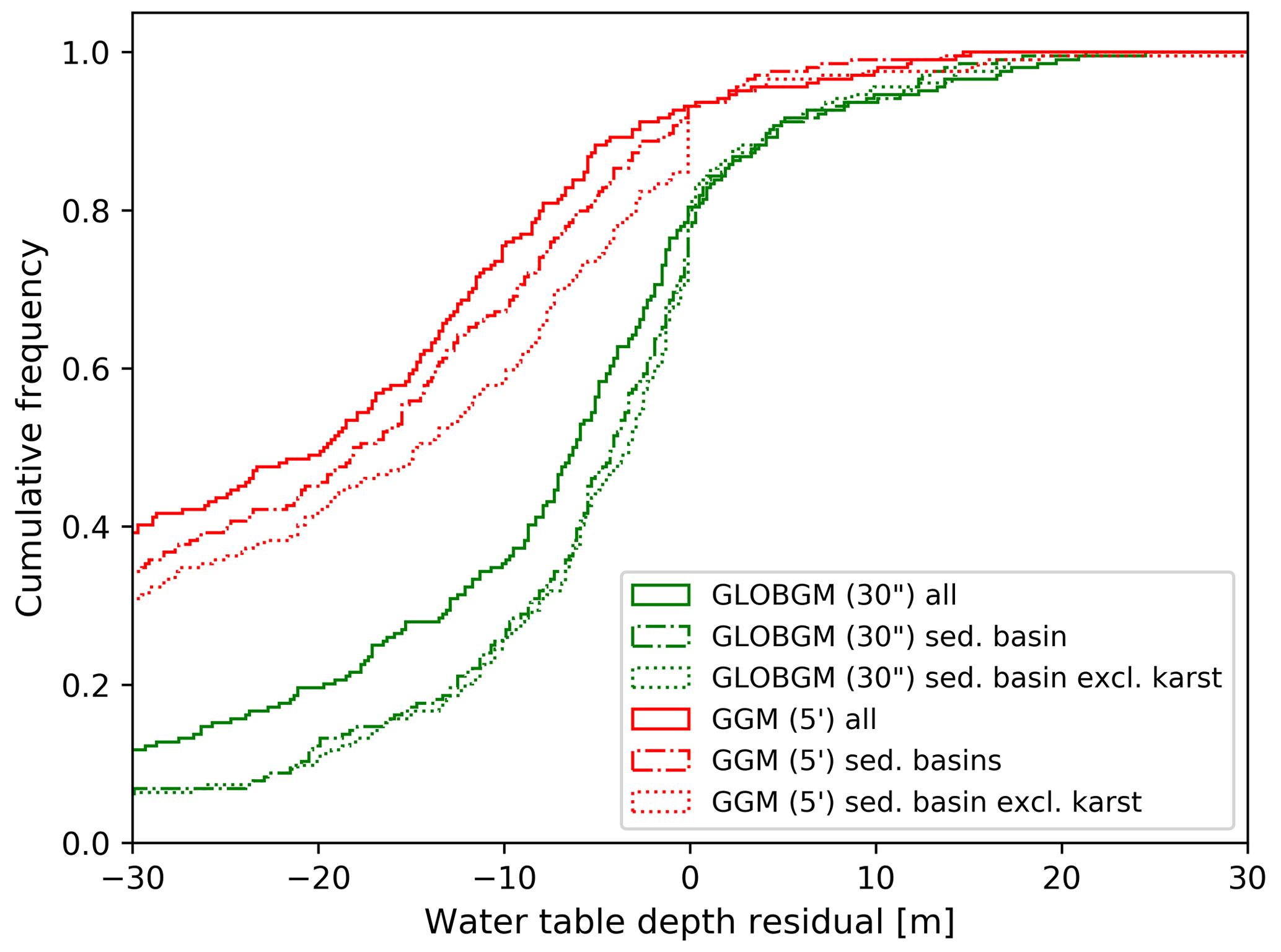
Figure A1 Cumulative frequencies of water table depth residuals aggregated to HUC4 units for the steady-state evaluation considering GLOBGM (green lines) and the GGM (red lines). The solid line includes all NWIS wells, similar to Fig. 13b. The dashed–dotted line is for NWIS wells only in sedimentary basins. The dotted line is for NWIS wells only in sedimentary basins excluding karst.

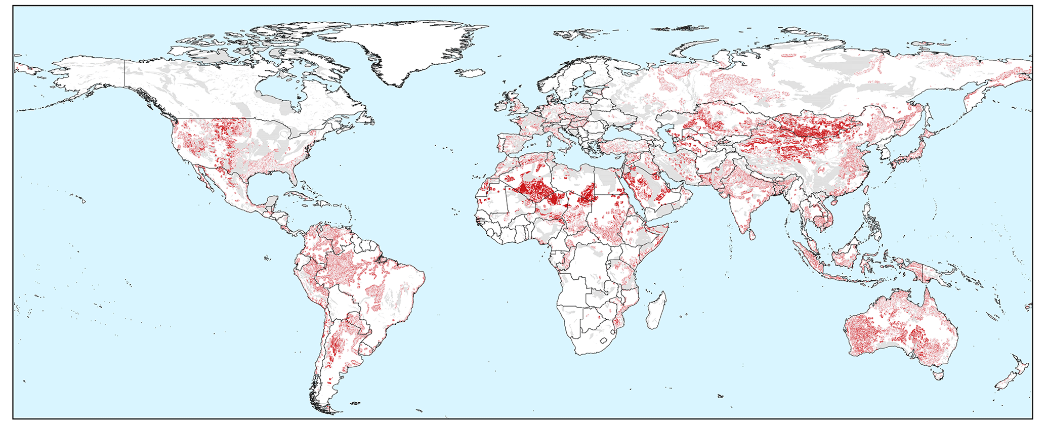
Figure A2 Locations (red) where groundwater seepage occurs from the lower model layer towards the upper model layer.