the Creative Commons Attribution 4.0 License.
the Creative Commons Attribution 4.0 License.
 | 12 Apr 2024
Inferring the tree regeneration niche from inventory data using a dynamic forest model
Florian Hartig
Harald Bugmann
The regeneration niche of trees is governed by many processes and factors that are challenging to determine. Besides a species's geographic distribution, which determines if seeds are available, a myriad of local processes in forest ecosystems (e.g., competition and pathogens) exert influences on tree regeneration. Consequently, the representation of tree regeneration in dynamic forest models is a notoriously complicated process which often involves many subprocesses that are often data deficient. The ForClim forest gap model solved this problem by linking species traits to regeneration properties. However, this regeneration module was never validated with large-scale data. Here, we compare this trait-based approach with an inverse calibration approach where we estimate regeneration parameters directly from a large dataset of unmanaged European forests. The inverse calibration was done using Bayesian inference, estimating shade and drought tolerance as well as the temperature requirements for 11 common tree species along with the intensity of regeneration (i.e., the maximum regeneration rate). We find that the parameters determining the species' light niche (i.e., light requirements) are similar for the trait-based and calibrated values for both model variants, but only a more complex model variant that included competition between recruits leads to plausible estimates of the drought niche. The trait-derived temperature niche did not match to the estimates from either model variant using inverse calibration. The parameter estimates differed between the complex and the simple model, with the estimates for the complex model being closer to the trait-based parameters. In both model variants, the calibration strongly changed the parameters that determine regeneration intensity compared to the default.
We conclude that the regeneration niche of trees can be recovered from a large forestry dataset in terms of the stand-level parameters light availability and regeneration intensity, while abiotic drivers (temperature and drought) are more elusive. The higher performance (better fit to hold out) of the inversely calibrated models underpins the importance of informing dynamic models by real-world observations. Future research should focus on even greater environmental coverage of observations of demographic processes in unmanaged forests to verify our findings at species range limits under extreme climatic conditions.
- Article
(5438 KB) - Full-text XML
- BibTeX
- EndNote


Predictions of species range shifts and forest dynamics under climate change require process-based models that account for the complex feedback between stand dynamics, soils, and climate (Morin and Thuiller, 2009). In this context, tree regeneration is particularly important because of its key roles in species range shifts (McDowell et al., 2020) and forest resilience to climate change (i.e., reorganization after disturbances; Seidl and Turner, 2022). Yet, tree regeneration is an uncertain and convoluted process (Price et al., 2001; König et al., 2022), as shown by numerous studies that yield different results depending on the site, species, and spatial and temporal scales that are considered (Clark et al., 1999; Lett and Dorrepaal, 2018). The reasons for these divergences between observations and experimentation are that (a) many seemingly stochastic regeneration processes are actually controlled by biotic and abiotic conditions that vary across a wide range of temporal and spatial scales (Grubb, 1977; Hart et al., 2017) and (b) there is a lack of suitable data for consistently studying these processes on different scales (Clark et al., 1999).
A challenge that hinders progress on these questions is that a tree's regeneration niche is generally driven by many factors and lacks a clear definition that distinguishes it from a plant's full niche (Grubb, 1977). Instead, differences between Grubb's niche types are continuous (see also ontogenetic shifts in environmental preferences; Heiland et al., 2022) and valid only conceptually. At the same time, Grubb's definition of the regeneration niche as “an expression of the requirements for a high chance of success in the replacement of one mature individual by a new mature individual of the next generation […]” provides a coherent framework to which regeneration models can be related.
Regeneration in most dynamic forest models (DFMs) is captured in a relatively simple manner (compared to the growth and mortality of adult trees) and, due to the lack of detailed process data, mostly phenomenologically (König et al., 2022). Nevertheless, even these simplified representations of tree regeneration are characterized by widely different levels of complexity (Bugmann and Seidl, 2022). Typically, the representations of regeneration in DFMs are based on knowledge that is abstracted to an aggregate over many processes (Price et al., 2001). DFMs usually simulate regeneration via binary, count, or hurdle models. Such probabilistic models simulate the occurrence of small trees at certain size thresholds as a function of environmental variables and sometimes dispersal, vegetative reproduction, or browsing. The complexity of these models is characterized by the different definitions of the relation between environmental variables and the species' regeneration probability. Consequently, there is a wide range from very simple models that use binary threshold values for one or very few variables (e.g., FORMIND; Köhler and Huth, 1998) to highly complex models with continuous transitions from unsuitable to suitable regeneration conditions comprising many variables (e.g., iLAND; Seidl et al., 2012). In addition, the actual regeneration amount is often calculated invoking random numbers, which leads to high stochasticity and renders the validation of tree regeneration patterns in DFMs challenging. Bugmann and Seidl (2022) and Hanbury-Brown et al. (2022) provide a comprehensive overview of regeneration models.
In this study, we focus on the relation between the tree species' regeneration success and environmental variables in DFMs. For this purpose, we aim to disentangle the effects of large- and small-scale environmental drivers on tree regeneration based on regeneration data that stem from natural conditions, i.e., unmanaged forests. In conjunction with such data, DFMs can be used to assess how simulated natural regeneration relates to real-world observations. First, DFMs represent complex stand–environment feedbacks explicitly, which places the quantified effects in the context of specific processes. For example, species shade tolerance estimates will only be constrained by the actual available light and not by any other confounding factors. This opens up opportunities for more nuanced inference on processes instead of yielding loose associations between observed regeneration patterns and environmental drivers. Second, using data from unmanaged forests minimizes the confounding influence of management on demographic processes. Specifically, the promotion of certain species or individual trees through planting or thinning is absent in unmanaged forests.
Over the past decade, robust methods for evaluating stochastic models of ecological processes with data have been developed (see Hartig et al., 2011). Yet, only a few studies have compared tree regeneration models with forest inventory data (Rüger et al., 2009; Díaz-Yáñez et al., 2024). An important reason for this is the issue of elucidating the drivers of ecological processes at different spatial and temporal scales mechanistically, as the apparent stochasticity makes it challenging to retrieve the signal from the data (Hart et al., 2017; Oberpriller et al., 2021; Shoemaker et al., 2020). Specifically, trade-offs between meaningful observations for key small-scale processes, such as light competition, browsing, microclimate (e.g., frost events), and the coverage of macroclimatic gradients at which dispersal and plant migration take place, impede a comprehensive analysis across the stages of tree regeneration (Clark et al., 1999). Consequently, there is a need to advance the frontier of evaluating tree regeneration in DFMs with data (see Díaz-Yáñez et al., 2024).
In the DFM ForClim (Huber et al., 2020), which we use as a case study, the regeneration niche is captured, among other factors, based on light availability, water availability, and summer temperature conditions. It is derived from trait values for shade tolerance, drought tolerance, and minimum degree-days (e.g., Leuschner and Ellenberg, 2017). The model is highly sensitive to the values of these parameters (see Huber et al., 2018), which adds weight to their detailed evaluation based on real-world observations. For traits directly linked to a specific explicitly modeled process, such as the relationship between the species' shade tolerance and light availability, a higher predictive power is anticipated. In contrast, traits influencing multiple processes tend to exhibit lower predictive power. An example of this is the intricate relationships involving the species' temperature requirements, frost tolerance, and drought tolerance, all of which interact with factors such as precipitation and temperature (see Yang et al., 2018). Functional traits have been successfully applied in simple dynamic models of annual plant communities (e.g., Chalmandrier et al., 2021), thus underpinning the validity of trait-based approaches for modeling plant demography.
In ForClim, the interplay between the traits of multiple species is implemented in two variants, i.e., a simple and a complex approach for capturing regeneration processes. In the simple approach, the relation between traits and environmental conditions is defined using binary thresholds and competition among regenerating trees is not considered. In the complex approach, the relation between traits and environmental conditions is defined with continuous transitions between suitable and unsuitable regeneration conditions, and competition among regenerating trees is considered (Huber et al., 2020). Interestingly, in both variants, the link between traits and processes leads to ecologically plausible emergent properties of simulated potential natural vegetation along elevational gradients in the Swiss Alps (Huber et al., 2020) and elsewhere (Bugmann and Solomon, 2000). While empirical studies based on plot-level data have provided valuable insights into large-scale regeneration patterns (Zell et al., 2019; Käber et al., 2021), it remains unclear whether DFMs can match such empirical data. A comparison of many DFMs with data on unmanaged European forests shows that mismatches exist; yet, the reasons for these mismatches remain vague (Díaz-Yáñez et al., 2024).
Here, we evaluate possible reasons for mismatches between process formulations and observations by comparing two approaches for parameterizing the regeneration niche in ForClim: (1) a trait-based approach, where the regeneration niche is based on trait values determined a priori from ecological knowledge, and (2) an inverse calibration approach, where the trait values are derived a posteriori using a novel observational dataset of demographic processes in European unmanaged forests that covers unprecedented spatial and temporal scales (Käber et al., 2023). Specifically, we address two research questions:
-
How does the regeneration niche that emerges from the inverse calibration differ compared to the niche defined by the species' traits?
-
Does a more complex regeneration model that includes competition feature a higher performance compared to a simple regeneration model without competition?
2.1 Data
2.1.1 Forest inventory data
We used records of tree recruitment from 6540 forest inventory plots covering 299 strict forest reserves that are curated by 18 European research institutions in the context of the European Forest Research Initiative (EuFoRIa, https://www.euforia-project.org, last access: 15 September 2023) (Käber et al., 2023). Depending on the forest inventory design, different diameter thresholds (DBH, diameter at breast height) were used as the calipering limit in the inventories (i.e., 4, 7, or 10 cm). These inventory plots were aggregated or split into units of ca. 1 ha to obtain samples of a similar spatial extent (Käber et al., 2023), which reduces the stochasticity in the data and thus increases the stability of the signal used for model evaluation. After data processing (Käber et al., 2023), 865 plots were available for this study. Some trees within these plots had implausible DBH measurements (e.g., annual DBH growth was unrealistically high (ΔDBH > 2 cm yr−1) or negative (ΔDBH < −0.1 cm yr−1)), which required the exclusion of some plots. This allowed us to obtain a dataset where all observations are in an ecologically plausible range.
We defined two criteria for selecting plots suitable for the study. The first criterion evaluated the number of trees with implausible measurements relative to the total number of measured trees and observed basal area: at least 95 % of all trees needed to have plausible measurements and at least 95 % of the basal area comprised trees with plausible DBH measurements. The second criterion evaluated the number of trees with implausible measurements relative to the plot area: the maximum number of trees with implausible measurements per ha allowed in the dataset was defined as the 75th percentile of trees with implausible measurements per ha (which amounted to 14.31 ha−1). The second criterion was defined because some plots did not fulfill the first criterion, although they had a relatively low number of trees with implausible measurements per ha. These were particularly large plots with a low tree number per ha (N=51). After plot selection, all trees with implausible DBH measurements of the selected plots were removed.
The final number of sites considered was 696, which provided sufficient information on tree regeneration for 11 tree species. All other species were aggregated in an extra category (“other” species). About half of the sites (353) were used for calibration (training data), and the other half (343) were used for evaluation (test data). We split the sites so that the variation of the represented inventory datasets (i.e., the individual data associated with one research institution) and DBH thresholds was similar in both test and training data. This also resulted in similar variations of environmental conditions because each inventory dataset (from a given institution) represents a specific region with similar environmental conditions.
2.1.2 Environmental input data
ForClim contains a stochastic weather generator where the long-term averages and standard deviations of monthly mean temperature and log-transformed precipitation sums, along with their cross-correlation, serve as input (Bugmann, 1994; Risch et al., 2005). These climatic input variables were derived from the CHELSA dataset version 2 (Karger et al., 2017) with a horizontal resolution of 30 arcsec. The plot's slope and aspect (represented as “kSlAsp” in the model; Bugmann, 1994) are input variables as well; they were derived from the Copernicus digital elevation model EU-DEM (EU-DEM 2020) with a spatial resolution of 25 m, which was further processed with QGIS (QGIS Development Team, 2022) to calculate the slope and aspect with a spatial resolution of 100 m. The so-called “bucket size”, i.e., the plant-available water storage capacity of the soil, was derived with a random forest model trained with expert assessments of the soil quality of a subset of the plots (see Käber et al., 2023).
2.2 The forest gap model ForClim
ForClim is a dynamic vegetation model that simulates the processes of growth, mortality, and regeneration (often also called “establishment”) of individual trees via species-specific size cohorts (Bugmann, 1994). ForClim is classified as a forest gap model (Shugart, 1984) and simulates forests in independent patches, each with a size of 800 m2. By default, 100 patches (i.e., 8 ha) comprise a forest stand, which is used to obtain realistic averages of forest dynamics across patches. The model uses an annual time step and represents trees as cohorts with the properties number of trees (Trs), diameter at breast height (DBH), height, leaf area, and stress level. Here, we used two variants of the regeneration module within ForClim v4.0.1 (Huber et al., 2020).
2.2.1 The two regeneration models
The ForClim regeneration module initiates new cohorts of trees based on (a) site variables for climate and soil in combination with (b) species traits and (c) state variables of forest structure. The species traits of drought tolerance, temperature, and light requirements originate from the indicator values of Ellenberg (1986) (see the latest translated edition, Leuschner and Ellenberg, 2017) and the FORECE model (Kienast, 1987). They define thresholds (so-called “establishment flags”, EFs) that must be fulfilled for a species to qualify for establishment at a DBH of 1.27 cm. For example, if a species has an EF of 10 % of the available light to regenerate, the EF will be fulfilled if the available light is ≥ 10 %. If the available light is < 10 %, the species EF is not fulfilled (see the detailed description of establishment flags below). In this study, we focus on a simple variant and a more complex variant of the regeneration model. Below, a brief summary of the two models is provided, followed by an explanation of the EFs investigated here. For more details, see Fig. 1, Appendix B, and the original documentation for the simple and complex models in Bugmann (1994) and Huber et al. (2020), respectively.
The simple model simulates tree regeneration for each species independently and corresponds to the original ForClim establishment module in Bugmann (1994), which is the same as model variant 1 in Huber et al. (2020). EFs in this model indicate either “suitable” or “not suitable”; i.e., they are binary. In a first step, the annual regeneration probability (kEstP), modulated by species-specific EFs, determines whether regeneration takes place for each species. Second, if the regeneration of a species takes place, the potential maximum number of new trees for that species is calculated from (1) a regeneration intensity parameter (kEstDens, which is the maximum tree establishment density per species [m−2 yr−1]), and (2) the species-specific successional strategy (i.e., shade-tolerant species have a higher number of seeds and thus offspring compared to shade-intolerant species). Third, the actual number of new trees per species is derived by drawing a random number between 1 and the potential maximum number of trees for each species.
The complex model includes a mechanism for competition and was first introduced as variant 11 in Huber et al. (2020). EFs in this model are continuous, which allows for a more nuanced gradient from “suitable” to “not suitable”. In the first step, kEstP, as modulated by a drought index and degree-days, is used to determine if regeneration takes place for any species. Second, if regeneration does take place, the total potential number of new trees over all species is calculated from (1) a regeneration intensity parameter (kTrMax, which is the absolute maximum number of trees [ha−1]) and (2) a drought index, degree-days, and the continuous EFs. The actual number of new trees over all species is then derived by drawing a random number between 1 and the potential maximum number of trees over all species. Third, the number of new trees per species is calculated by multiplying the actual number of trees over all species by the species-specific ratio of each species' EF and the sum of the EFs of all species.
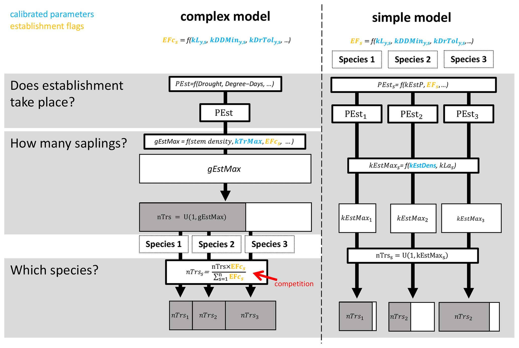
Figure 1Simplified visual representation of the simple and complex regeneration model variants of ForClim. A full description of the models is provided in Sect. 2.2 below.
2.2.2 Establishment flags regarding light, temperature, and soil moisture
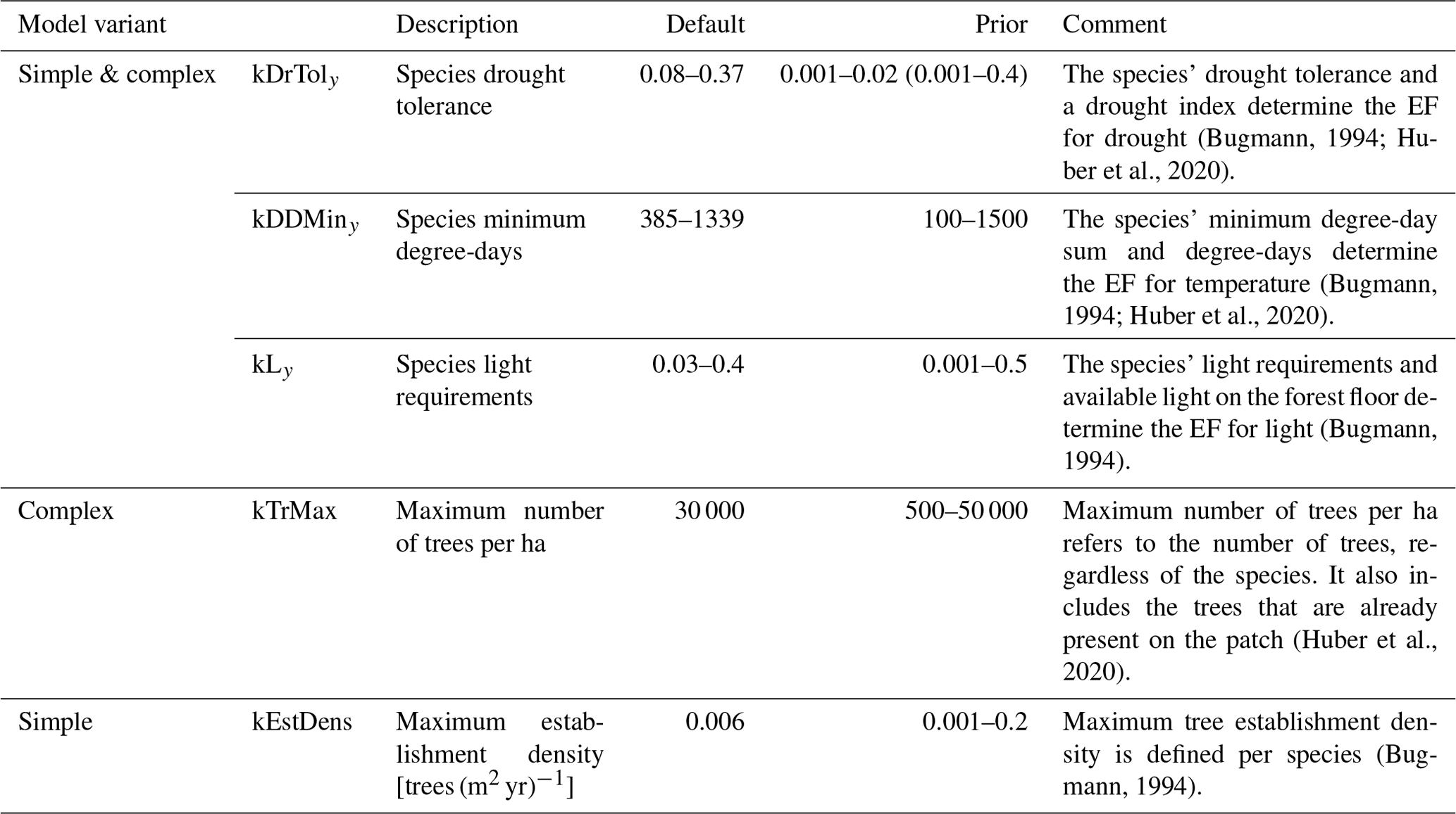
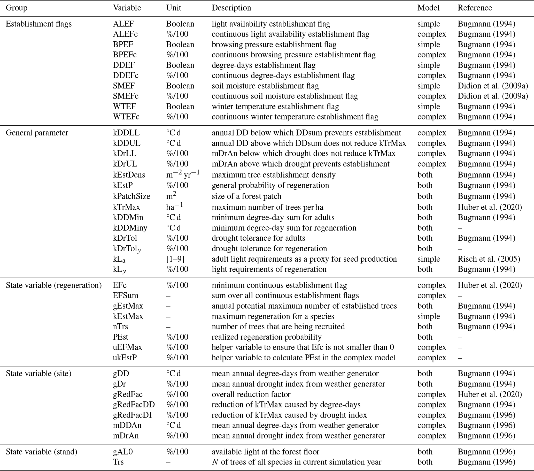
In the present study, we focus on three of the five EFs that are used in the two models (Table 1). The definitions of these three EFs (for light, drought, and degree-days) are given below.
The available light establishment flag (ALEF) evaluates whether the sunlight available at the forest floor (gAL0; see p. 63 in Bugmann, 1994 for details) matches a parameter for the species' light requirements to regenerate (kLy,s). kLy,s is derived from indicator values (ranging from 1 to 9) regarding the light requirements of young trees (Ls) (Leuschner and Ellenberg, 2017). Here,
For each species s, the binary EF (ALEFb,s) in the simple model is calculated with
while the continuous EF (ALEFc,s) in the complex model is calculated with
where the value 0.5 refers to the highest kLy,s (see Eq. 1) and serves as a buffer for the transition from 0 to 1.
The degree-days establishment flag (DDEF) evaluates whether the annual degree-day sum (gDD; see p. 81 in Bugmann, 1994 for details) matches the species' minimum degree-day requirement (kDDMin). The values of kDDMin originate from Kienast (1987), who derived climatic variables from Müller (1982) and Rudloff (1981) for multiple geographic locations and elevations within the species' distribution range (Ellenberg and Klötzli, 1972; Meusel et al., 1965). This approach was further improved by applying a site-specific bias correction (Bugmann, 1994). Note that this parameter has never been modified to reflect possible deviations regarding the regeneration niche. In this study, we distinguish between the original parameter (kDDMin of adults) and kDDMiny, which applies to the regeneration. For each species s, the binary EF (DDEFb,s) in the simple model is calculated with
while the continuous EF (DDEFc,s) in the complex model is calculated with
where the value 256 refers to the lowest kDDMiny,s and serves as a buffer for the transition from 0 to 1.
Lastly, the soil moisture establishment flag (SMEF) evaluates whether the drought index (gDr), defined as the ratio of actual evapotranspiration and water demand by the atmosphere (i.e., potential evapotranspiration), matches the species' threshold for this index, i.e., the drought tolerance (kDrTol). The original trait values for drought tolerance range from 1 to 5 (Leuschner and Ellenberg, 2017) and were scaled between 0.06 and 0.3 (i.e., 30 %). The evolution of the formulation of the drought index, including its integration into the regeneration model (Didion et al., 2009a), is documented in Bugmann (1994), Bugmann and Cramer (1998), and Bugmann and Solomon (2000). Similar to the DDEF, the original parameter (kDrTol of adults) and kDrToly are distinguished here, and the latter applies to regeneration only. For each species s, the binary EF (SMEFb,s) in the simple model is calculated with
while SMEFc,s in the complex model is calculated with
where the constant of 0.08 indicates the lowest kDrToly,s and serves as a buffer for the transition from 0 to 1, i.e., the EF being fulfilled or not (see Huber et al., 2020).
The two EFs in the model that are not considered here are the winter temperature establishment flag (WTEF), which depends on the minimum tolerated winter temperature and chilling requirements (Bugmann, 1994; Bugmann and Cramer, 1998; Kienast, 1987), and the browsing pressure flag, which depends on the species' susceptibility to ungulate browsing (Didion et al., 2009b). WTEF is correlated with DDEF and excluded from the calibration to avoid too many degrees of freedom. We therefore used the default parameterization for WTEF. Because no site information on browsing pressure was available, we decided against using this factor in the calibration. Instead, we kept browsing pressure constant across all sites at its default value of 20 %.
Table 1Description of ForClim model parameters that are considered for calibration.
2.3 Calibration approach
We used Bayesian inference to estimate the unknown parameters of the two ForClim regeneration models and their uncertainties. We estimated three species-specific (kLy,s, kDDMiny,s, and kDrToly,s) and two general (kEstDens, kTrMax) regeneration parameters of ForClim based on recruitment data from the EuFoRIa reserves. The species parameters were estimated for 11 out of 30 simulated species for which the data covered sufficient environmental variation. The species not considered for calibration were simulated with their default parameters (see Huber et al., 2020).
2.4 Calibration target
The calibration target was to obtain recruitment rates in the model that match to observations. Tree recruitment was quantified as the number of trees that pass an inventory-specific DBH threshold. Observed decadal tree recruitment rates Ri,s were calculated for each plot i and species s with
where p is the inventory period and Ti is the total number of years between the first and the last inventory at plot i. Simulated tree recruitment rates were calculated as
where is the number of recruited trees for one patch j, inventory period p, and repetition k. Each simulation during the calibration was conducted on > 100 patches (i.e., ca. 8 ha) to reduce the variability caused by the k stochastic realizations of the ForClim model. The trees in the initial forest inventory were randomly distributed to each of the 100 patches (each with a size of 0.08 ha) proportionally to the actual plot size until a full repetition exceeded 100 patches. If one repetition was not a multiple of the patch size of 0.08 ha, the difference in exceeded plot area determined the proportion of additional trees drawn from all trees in the initial forest inventory to populate the patches. The number of repetitions Nrepi for each plot i emerges from the next integer above , where Ai is the plot size in ha. This resulted in an average of eight repetitions k across all sites, although k ranged from 40 for plot sizes of 0.2 ha to 2 for two sites with plot sizes of > 4 ha. The number of patches j () within one repetition k is the next integer above .
2.5 Model initialization
To initiate the calibration runs, we had to resolve the issue that trees below the inventory-specific DBH threshold (i.e., small trees), which may have been present in reality, are obviously not present in the data. Ignoring these trees in the initialization would create a temporal lag in tree recruitment (i.e., trees surpassing the DBH threshold), which is connected with a potentially significant underrepresentation of tree regeneration directly after model initialization. To overcome this problem, we initialized unobserved trees below the DBH threshold with the model's steady state (i.e., equilibrium of regeneration).
This steady state was determined by running the simulation with the stand structure of the initial forest inventory for 50 years and suspending all processes affecting trees above or equal to the DBH threshold. During this “spin-up” phase, trees above the DBH threshold that were included in the initial forest inventory could neither die nor grow, but they still modulated the variables of stand structure that affect regeneration (i.e., gAL0, Trs). In contrast, trees below the DBH threshold were allowed to grow and die under the conditions observed in the initial inventory. If these newly regenerated trees grew larger than the DBH threshold during the spin-up, they were removed. This means that these trees did not die from mechanisms that simulate tree mortality in the model; they were forcefully removed from the simulation to avoid the accumulation of trees with a DBH close to the DBH threshold. Visual inspection of the simulation results showed that an equilibrium of the stand structure below the DBH threshold was reached after approximately 50 simulation years, which was the reason to fix the spin-up at this time period. After the spin-up, the simulation was continued with all trees and by running all model processes (i.e., regeneration, growth, and mortality).
2.6 Definition of goodness of fit
The goodness of fit was quantified by a (pseudo-)likelihood. We assumed that the observations Ri,s for site i and species s with the parameter vector θ were negatively binomially distributed, leading to a log-likelihood per observation of
Here, the mean is predicted by ForClim based on the chosen values for the model parameters kLy, kDDMiny, and kDrToly, the respective regeneration intensity parameters (kEstDens and kTrMax) of the two models (as explained above), and the dispersion parameter ϕ of the negative binomial distribution, which can be interpreted as a measure of residual variation and is a free parameter that needs to be estimated in addition to the model parameters.
We assumed that the dispersion may vary with species, DBH, and plot size according to the formula
where ϕs is the species-specific dispersion, ϕDBH is the effect of the diameter threshold DBHi, and ϕA is the effect of the plot size Ai on the dispersion. We used an exponential function to only allow for positive values, as required by the negative binomial distribution. In sum, the likelihood depends on a parameter vector θ that includes the model parameters as well as the parameters that control the value of ϕ based on the DBH and plot size.
Summing the expressions in Eq. (10) over all plots i and over all species s, we arrive at the joint log-likelihood
We then additionally re-scaled the joint log-likelihood (Eq. 13) by a factor of (reflecting Nspecies) to arrive at a pseudo-likelihood that we used as the calibration target in our MCMCs.
The effects of this re-scaling are that the uncertainties get larger and the absolute magnitude of (stochastic) likelihood differences decreases. For both reasons, MCMC samplers are less prone to get stuck in local optima, whereas the shape of the posterior surface as well as the posterior optimum remain unchanged. However, the re-scaling (which essentially corresponds to a down-weighting of the observational evidence by a factor of 12) can be interpreted as accounting for possible non-independence of the data and structural model error (see Oberpriller et al., 2021). The value was chosen ad hoc, but, given that some structural error and non-independence are likely present in the observations, we believe it is of the right order of magnitude. Given the approximate nature of this correction, our scaled likelihood should be viewed as a pseudo-likelihood or an informal likelihood (Smith et al., 2008), and the same labels should be applied to the posterior.
In total, our pseudo-likelihood depends on a vector θ consisting of 48 parameters, as we estimated three ecological threshold parameters (kLy, kDDMiny, and kDrToly; see Fig. 1) and a separate dispersion parameter ϕs for each of the 11 species, one extra dispersion parameter for all other species, two parameters for the effects of DBH and plot area (ϕDBH and ϕA), and one parameter for the regeneration intensity (kEstDens or kTrMax for the simple or the complex model, respectively). We defined wide uniform priors for each parameter that comprise the full range from the species' lowest value to its highest value in the default parameterization in ForClim (see Table 1).
2.7 Posterior estimation
We calibrated the model using the differential evolution sampler (DEzs; ter Braak and Vrugt, 2008) implemented in the R package BayesianTools (Hartig et al., 2019). We sampled with two independent sets of three chains (i.e., a total of six chains) for all 353 training plots. The z matrix was re-initialized at the beginning of the sampling procedure (at 5000 to 6800 and 2000 to 3700 iterations for the simple model and the complex model, respectively) to improve the mixing of the chains. This was necessary because of the very wide prior range for the dispersion parameters, which led to a degenerate z matrix. The same procedure was applied to improve chain mixing after 120 000 to 139 300 (simple model) and 120 000 to 145 500 iterations (complex model). For the simple model, the upper prior range for the parameter kEstDens had to be adjusted from 0.02 to 0.2 after 139 300 iterations. Ultimately, after 191 600 (simple model) and 200 900 iterations (complex model), one set of three independent chains converged, as judged from a visual inspection of the chains and Gelman and Rubin's MCMC convergence diagnostic (see Table A4). The other set of independent chains did not fully converge, mostly because one chain was stuck for the species-specific dispersion parameters. Computational constraints did not allow us to run the sampler for even longer. A single simulation took 3 s per plot; i.e., 6 chains × 353 calibration plots resulted in a total computation time of 1.765 h per iteration without parallelization. Fortunately, the Euler High Performance Computing Cluster of ETH Zürich enabled us to use 1000 cores (500 per model variant) and sufficient memory. The effective computing time, including the overhead when utilizing all resources, was 10–15 s per iteration and ca. 25 d in total for each model variant.
The posterior distribution from the calibration consisted of 1000 samples drawn from the last 32 300 (simple model) and 45 400 (complex model) iterations. The simulations from the posterior parameter distribution provided posterior estimates of decadal tree recruitment rates () for all 343 test plots i and species s. The mean posterior estimate (MPE) and the 80 % credible intervals (CIs) of from the 1000 posterior simulations were used to assess residuals and evaluate model performance (see Table A4). The MPE and CIs for the parameter estimate of the posterior distribution were used to compare the trait-based model and the calibrated model.
2.8 Performance comparison using the RMSE and marginal pseudo-likelihood (ML)
Model performance was assessed with the RMSE and the marginal pseudo-likelihood (ML) on both training and hold-out data. The difference between the two metrics is that the RMSE is a general metric of fit, while the marginal pseudo-likelihood is a Bayesian metric that relates to the Bayes factor and posterior model weights and thus allows the support for two alternative models to be compared based on a specific likelihood.
For the simulations from the calibrated and trait-based models, the RMSE was calculated for different DBH thresholds: for variable thresholds between plots and harmonized DBH thresholds of 7 and 10 cm. This harmonization was done by artificially increasing the DBH threshold in the observed and simulated data to mimic a consistent inventory design with a common DBH threshold. We calculated the RMSE from the training and test data based on a comparison of observed and simulated recruitment in terms of the species-unspecific, the species-specific, and the average over the species-unspecific and species-specific RMSEs (Table 2).
The ML was calculated only for the simulations of the calibrated models because the pseudo-likelihood relies on the dispersion parameters, which were not estimated for the trait-based model. The ML is the average pseudo-likelihood of the model given the training or the test data and is averaged over the posterior parameter uncertainty (see Delpierre et al., 2019). We evaluated the ML in both cases on the validation data based on the posterior distribution inferred from the training data. This approach, which corresponds to the fractional Bayes factor (O'Hagan, 1995), avoids inconsistencies when comparing models with weak or uninformative priors. The Bayes factor is then obtained by taking the ratio between two marginal likelihoods with eM1−M2. This provides the relative posterior support of M1 relative to M2 by the data (Kass and Raftery, 1995).
When interpreting the results, it is important to remember that both the RMSE and the ML, as evaluated here, will typically be higher for more complex models of the training data, so the comparison of models with these metrics of the training data is of limited use. However, models can be sensibly compared by comparing their performances for the hold out, and it is also informative to look at the reduction in performance between training and the hold out, which gives an indication of overfitting.
2.9 Posterior sensitivity
Global sensitivity analyses allow for the assessment of model behavior across large parameter spaces. However, large parameter spaces may also cover unrealistic parameter configurations, and computational requirements are high. Therefore, a strategy for constraining the parameter space to a relevant location is required (see Huber et al., 2018). We combined the benefits of a global and a local sensitivity analysis by constraining the parameter space by deriving a posterior distribution from the observations. This allowed us to evaluate model sensitivity with respect to the uncertainty derived from observed recruitment patterns in European forest reserves.
To analyze the sensitivity of regeneration to changes in the model parameters within the posterior distribution, we analyzed the effect of increased tolerance of trait values (i.e., a lower kLy, higher kDrToly, and lower kDDMiny) on simulated recruitment within the posterior parameter range. This was done by modeling with a GLM and a negative binomial distribution with z-scaled values of negative kLy, negative kDDMiny, and positive kDrToly as predictors. This model was implemented using glmmTMB (Brooks et al., 2017).
3.1 Species traits and regeneration intensity
The trait-based regeneration niche differs from the regeneration niche that emerges from the model which was calibrated with the observations made in unmanaged forest reserves. Variation in these differences is evident between trait types, species, and model variants (Fig. 2 and Table A2).
Light requirements stand out from the other traits because they were most sensitive during model calibration, as indicated by the narrow posterior distributions compared to the prior parameter range (Fig. 2, left; Fig. A2a). Most posterior estimates were not only narrow but also supported by the trait values (Fig. 3, left). Estimates of the complex model were generally closer to the trait values, with a good rank correlation (i.e., Spearman's rho = 0.57). Light requirements defined by traits for the simple model were systematically lower compared to the values emerging from the calibration. Nevertheless, a Spearman's rho of 0.94 indicates that the calibration put the species in a plausible order (Fig. 3, top left). The estimates of the species-specific light requirements were more similar for both approaches for shade-tolerant tree species in general. Values from the calibration for Quercus spp., Pinus sylvestris, and Betula spp. were much lower compared to the trait values in the complex model but were more similar in the simple model. For Tilia cordata, the calibration led to much higher light requirements compared to the trait-based values with either model (see Fig. 2, left). Drought tolerance values from both approaches matched moderately well when using the complex model (Spearman's rho = 0.46) with a relatively large CI, and the expectation was within the CI for eight species (Fig. 2, center). The MPE from the calibration was close to the definitions of the trait values for five species. However, drought tolerance estimates from the calibration did not match the trait values well for the simple model (Spearman's rho = −0.18). Only for six species did the wide CIs include the trait-based values, and the MPE matched the trait values in the simple model for two species only. For Quercus spp. (complex model), Tilia cordata (simple model), and Pinus sylvestris (both models), the calibration led to much lower values compared to the trait values. Conversely, for Alnus glutinosa and Fraxinus excelsior, the calibration resulted in higher values compared to the trait-based values (see Fig. 2, center).
Estimates for the minimum degree-days had a wide CI for both models and a low rank correlation between the approaches (Spearman's rho = 0.19 for the complex model and −0.3 for the simple model; Fig. 2, right). Although the posterior CI of the calibration included the trait-based values for many species, the intervals were wide and the MPE values were close to the trait-based values for only two and three species in the complex and simple model, respectively. This indicates that the calibration values neither fully disagree nor perfectly match the trait-based values. For Tilia cordata (both models) and Carpinus betulus (simple model), the calibrated values were much lower compared to the trait-based values. Conversely, the calibrated degree-day values for Pinus sylvestris (simple model) and Abies alba (both models) were considerably lower compared to the trait-based values (see Fig. 2, right).
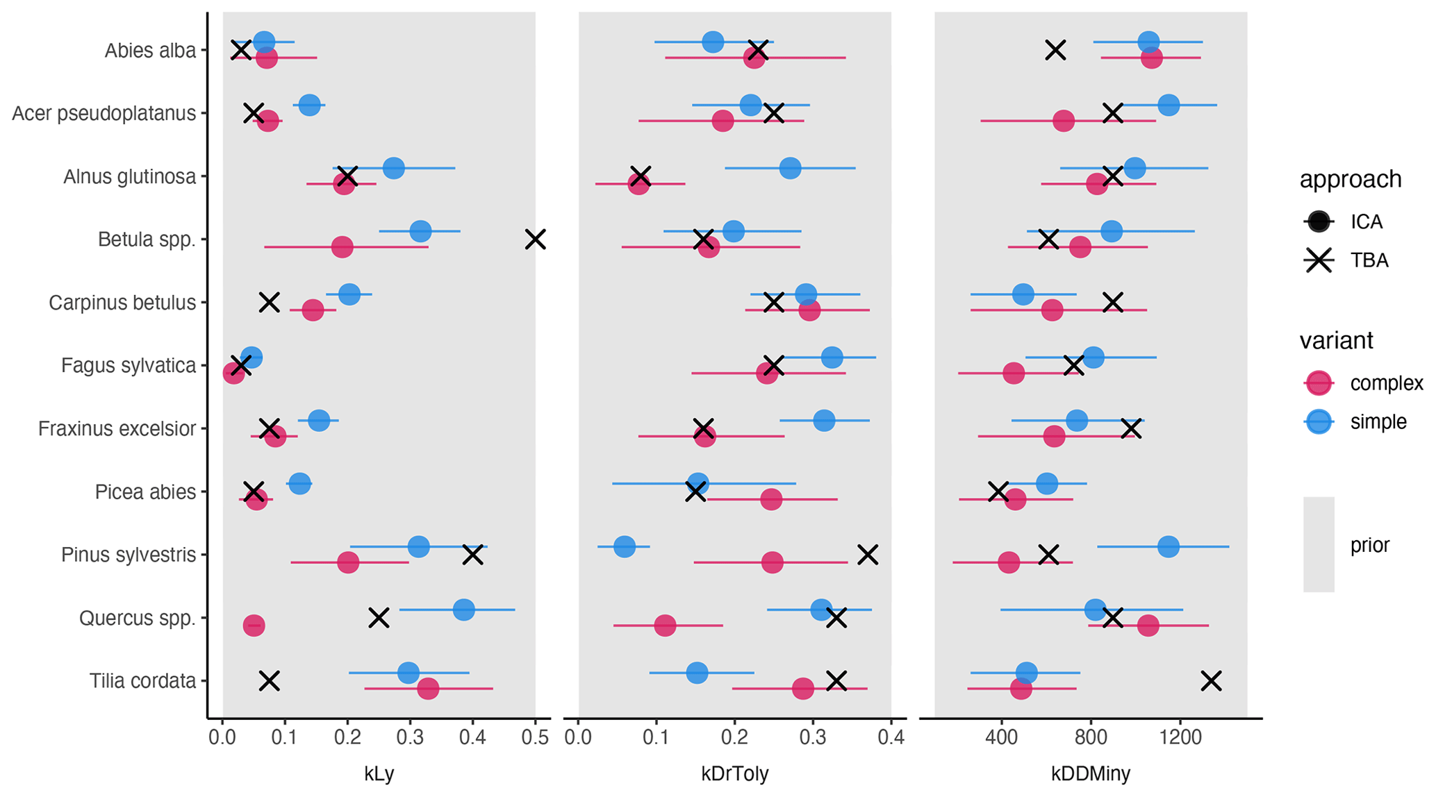
Figure 2Mean posterior estimate, including the 80 % CI, of the species-specific parameters for the complex model (red) and the simple model (blue). Point type indicates the approach (inverse calibration approach (ICA) or trait-based approach (TBA)). The panels show values for three species traits: light requirements (kLy), drought tolerance (kDrToly), and minimum degree-days (kDDMinkLy). The uniform prior parameter range (min, max) of each species trait (x axis) is indicated by the gray rectangle in the background.
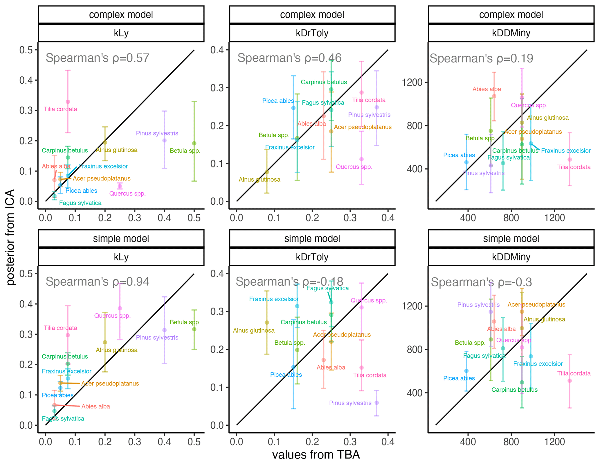
Figure 3Comparison of expected values for species-specific establishment thresholds based on ecological knowledge (TBA, trait-based approach; see Leuschner and Ellenberg, 2017) and MPE (ICA, inverse calibration approach; this study). The range displays the 80 % CI for the complex model (top panels) and the simple model (bottom panels). The 1:1 relationship is indicated by the black line. Spearman’s rank correlation of the MPE and the trait-based approach (TBA) values are shown in each panel.
The estimates of the calibration for general regeneration intensity were narrow compared to the prior (Fig. 4) and therefore considerably sensitive. While the species-unspecific parameter kTrMax from the calibration (complex model) was significantly lower than its default value for the trait-based model, the species-specific parameter kEstDens (simple) was higher than its default value for the trait-based model (Table A1). Considering the interaction between kEstP (which was reduced by a factor of ) and kEstDens or kTrMax (see the model description in Appendix B), the overall amount of regeneration is generally lower for the calibrated model compared to the trait-based model. Specifically, for the complex model, the MPE (kTrMax = 8762) suggests 25 times less maximum regeneration compared to the default values of the trait-based models (kTrMax = 50 000 × 5 = 250 000). For the simple model, the MPA (kEstDens = 0.022) suggests a reduction of ca. 24 % per species compared to the default trait-based model (kEstDens = 0.006 × 5 = 0.03). However, it is noteworthy that these parameters modulate regeneration differently and that the magnitude of the deviation between the parameters in the calibrated model, the default trait-based model, and the model variants is not directly translated into the simulated regeneration amount within the model (see Fig. 1 and the full set of equations in Appendix B).
The coefficient for the effect of the DBH threshold in the species-specific dispersion was significantly different from zero, with an MPE of −0.39 and −0.41 for the complex model and simple model, respectively. This indicates that dispersion increases for higher DBH thresholds (Fig. 4c). The coefficient for the effect of plot size is slightly negative but not significantly different from zero (Fig. 4d), which indicates that there is no significant effect of plot size on dispersion. However, a very weak positive effect of larger plots on dispersion is visible. At the species level, dispersion effects differed significantly, with the lowest dispersion seen for Fagus sylvatica and the highest for Quercus spp. (Fig. A1 and Table A3). These findings emerged from both the simple and the complex model (see Fig. 4c and d).
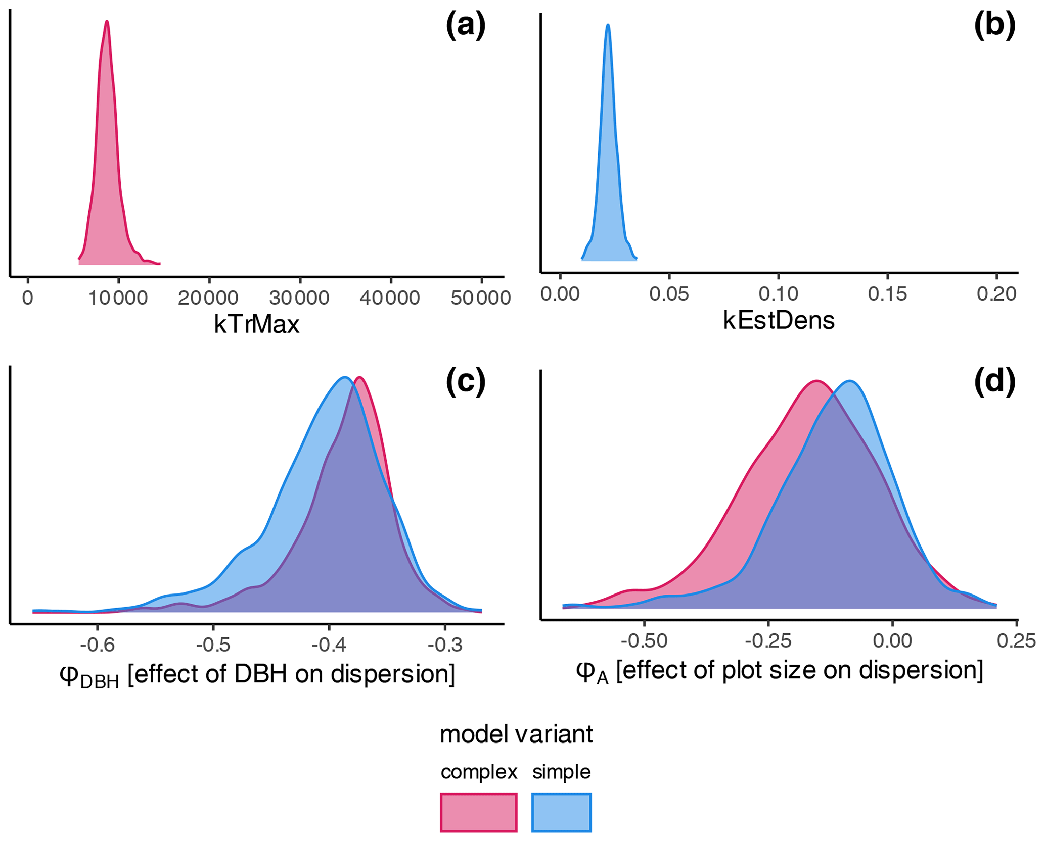
Figure 4Posterior distributions of the non-species-specific parameters determining the amount of regeneration: (a) kTrMax (complex model, red) and (b) kEstDens (simple model, blue). Effects on the dispersion parameter ϕ: (c) DBH threshold and (d) plot size. The prior parameter in (a) and (b) is given by the extent of the graph. The prior range for the dispersion parameters was −5 to 5 and is not shown. Note that lower values of the dispersion parameter indicate higher dispersion. Consequently, negative estimates for dispersion are positive effects on the actual dispersion. Species' dispersion parameters are presented in Table A3.
3.2 Model performance
The calibration led to somewhat better performance compared to the trait-based approach (Fig. 5 and Table 2). Both model variants performed better when calibrated and revealed the uncertainty of the posterior simulations. However, performance differed strongly between species. The most gains in performance coupled with a high degree of uncertainty were evident for Abies alba and Tilia cordata with both models (Fig. 5). No increase in performance was evident for Quercus spp. and Alnus glutinosa, although high uncertainty of the simulations was evident for Alnus glutinosa with the complex model. Slight but distinct gains in performance were found for Fagus sylvatica and Picea abies with the complex model. Note that not only the intercept for the comparison of observations and simulations but also the slope changed, which indicates that this was not only due to the regeneration intensity parameters. Overall performance increased distinctly for the complex model and considerably for the simple model (see the RMSE in Table 2). In summary, the calibration clearly improved model performance for almost all species in the complex model and to a limited extent in the simple model. In addition, the uncertainty based on the posterior parameter distribution was clearly visible in the simulations. The RMSE decreased with increasing DBH threshold (Fig. A3) for both models.
The ML confirmed the higher performance of the complex model (ML = −391.61) compared to the simple model (ML = −401.86), which was also evident from the RMSE (Table 2 and Fig. A2b). According to Kass and Raftery (1995), the fact that the Bayes factor from the training data is above 200 suggests strong support for the complex model (Bayes factor = 28 282.54).
Table 2RMSEs of the simulated and predicted R and the pseudo-likelihoods for the different models and approaches (the inverse calibration approach (ICA) and the trait-based approach (TBA)). The marginal pseudo-likelihood (ML) was derived from the posterior parameter distribution of the training data (N=353) and the test data (N=343). Species-specific RMSE values are presented in Fig. A4.
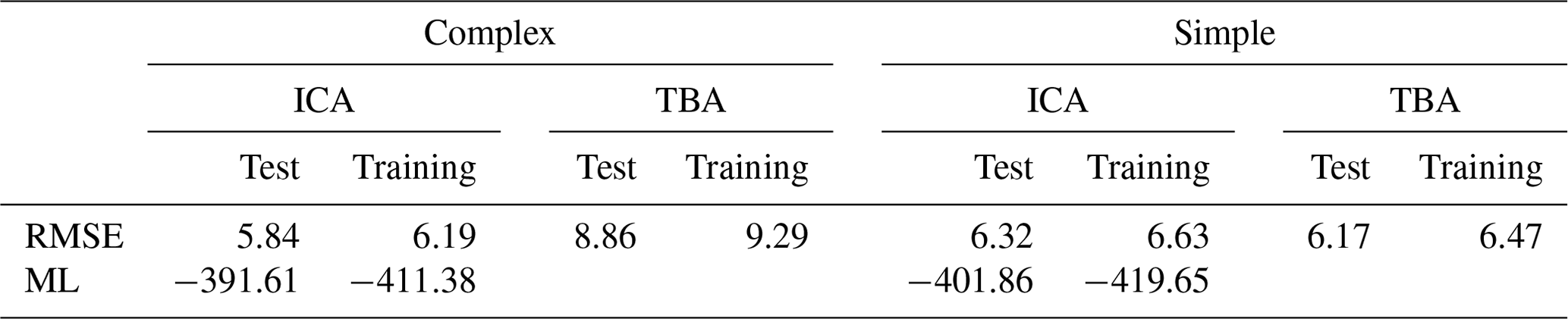
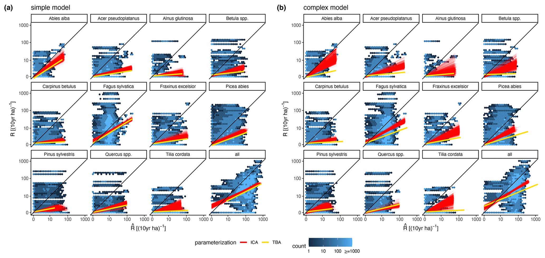
Figure 5Simulated vs. observed recruitment rates at 7 cm DBH of the 11 species for (a) the simple model and (b) the complex model. The red lines show linear regressions from 1000 simulated recruitment rates using the posterior parameter distribution at the 343 test plots. The data points used for the regression are indicated by the blue color of the hexagons, where light blue indicates fewer points and dark blue indicates more points. The yellow lines characterize the recruitment rates for the same test plots based on the default parameter setting (TBA, trait-based approach).
3.3 Posterior sensitivity
The variation of the parameter values characterizing the species' light requirements had the strongest effect on conspecific regeneration for each model variant (Fig. 6a and b, respectively). The variation of drought tolerance within the posterior, which was rather high, had a much weaker effect on conspecific recruitment, and the minimum degree-days had a very low effect on recruitment within the posterior parameter range. Interestingly, positive effects for heterospecific recruitment were evident in the case of higher shade tolerance of Quercus spp. and Acer pseudoplatanus, but only in the complex model (Fig. 6b). Picea abies (simple model) and Fagus sylvatica (complex model) showed the strongest negative effects on the emergence of heterospecific recruitment (Fig. 6).
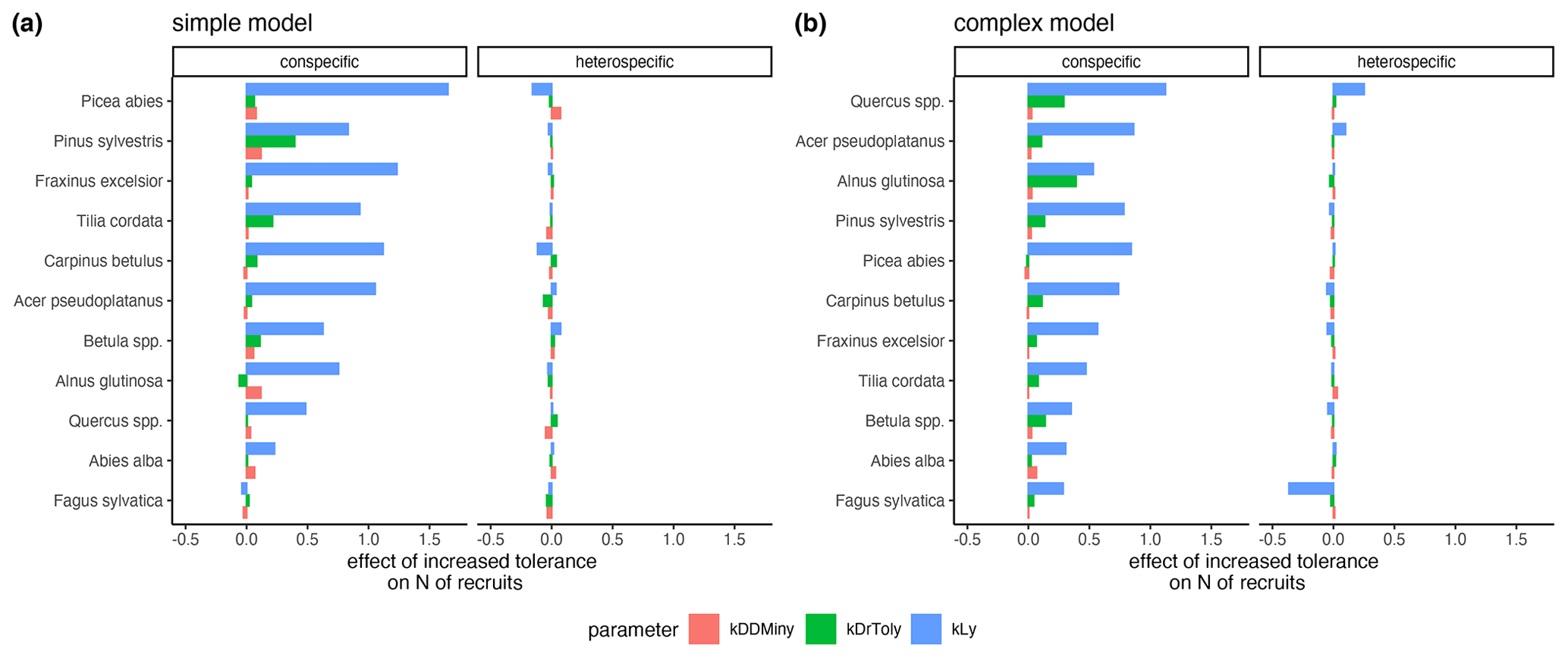
Figure 6Estimates of the effects of increased tolerances for kLy, kDrTolyy, and kDDMinyy on the emergence of conspecific and heterospecific recruitment for the simple model (a) and the complex model (b). The effect sizes correspond to the coefficients from a GLM that predicts recruitment with scaled tolerance parameters so that they have a mean of 0 and a standard deviation of 2; an increase in the value always indicates an improvement for the species.
Below, we discuss the research questions with respect to the results and the ecological implications of our findings. First, we focus on the differences in species-specific traits between the calibrated and the trait-based model; second, we evaluate how the structures of the simple and complex models affected performance; and third, we discuss technical advances and methodological aspects.
4.1 Species traits
The species trait values varied considerably between the calibrated models, the trait based-models, and the two model variants. We aim to explain these differences by reflecting on (a) the theoretical expectations of the two approaches and (b) the structural differences between the model variants.
Differences between the trait-based and calibrated models can be expected based on ecological considerations regarding the regeneration niche (Grubb, 1977) and ontogenetic niche shifts (Werner and Gilliam, 1984) as well as methodological aspects such as the importance of context for modeling trait–demography relationships (Yang et al., 2018). Specifically, we expected high sensitivity and a good match for the shade tolerance of the species because light availability is a key determinant of tree regeneration on small spatial scales (Collins and Good, 1987) and its context is modeled explicitly and in rather high detail in ForClim (note the direct link between stand structure and light availability in Eqs. 1 to 3). In contrast, the context of trait values related to climate (drought tolerance and temperature requirements) is only vaguely defined by species distribution limits (Meusel et al., 1965) along macroclimatic gradients (Rudloff, 1981). In addition, the traits for light requirements are differentiated between juveniles and adults (Leuschner and Ellenberg, 2017), while those related to climate are not. Therefore, we expected less agreement between the calibrated and trait-based models for the latter drivers. Our results supported these expectations, as shown by the mostly good agreement between the light requirement parameters compared to climatic parameters in the two approaches. Notably, this pattern was found in both the simple and the complex model, and it thus appears to be a robust feature, irrespective of the structure of the regeneration model. Furthermore, the drought-related parameters matched better between the calibrated and the trait-based models in the complex variant, which indicates that trait values embedded in a model that connects drought effects and competition during regeneration have more support from the data. This interlink of competition and drought has also been demonstrated in grassland communities (Grant et al., 2014; Levine et al., 2022) and tree species mixtures (Jucker et al., 2014; Grossiord, 2020; Young et al., 2017; Clark et al., 2016; Ruiz-Benito et al., 2013; Haberstroh and Werner, 2022).
4.1.1 Light
The nuanced differences between the model variants in terms of the estimates of the species' light requirements can be put in context with the regeneration intensity parameter. The calibrated trait values from the complex model were almost identical to the trait-based values for most species (Larcher, 1996; Lyr, 1992), whereas in the simple model, the light requirements were systematically lower in the calibrated compared to the trait-based models. This indicates that in the simple model, excessive recruitment levels (as embodied by the parameter kEstDens) were compensated for by erroneous light requirements (see Fig. 2). These inconsistencies may arise from the structure of the simple model, where the amount of recruitment is equal for all species that regenerate. Thus, the simple model lacks the flexibility to (a) generate an appropriate number of recruits for the dominant species and (b) lower the number of recruits for less dominant species. This explanation is supported by two other findings: the estimates of the light requirements for the often-dominant species Fagus sylvatica matched the trait-based values, while almost all other species had exaggerated estimates (Fig. 2); and the sensitivity of Fagus sylvatica to light within the posterior distribution was close to zero, while there was considerable uncertainty regarding the modulating effects of light for other species (Fig. 6). The light-demanding tree species Quercus spp., Pinus sylvestris, and Betula spp., along with Tilia cordata, did not match expectations either, which is in line with this pattern. These findings suggest that structural problems regarding competition for light in regeneration models of European forests can be exposed by the behavior of Fagus sylvatica. Thus, if the competitive dominance of Fagus sylvatica is not captured appropriately, a calibrated model is likely to compensate for this elsewhere.
In contrast to the absolute values for light requirements, the ranking of the species was more similar for the approaches for the simple model (Fig. 3). The lower rank correlation of the complex model is mostly due to much lower estimates for light-demanding tree species such as Betula spp., Pinus sylvestris, and Quercus spp., thus suggesting that the simple model performs better in simulating the regeneration of early-successional species. One possible reason for this behavior could be that all establishment factors (i.e., environmental drivers of regeneration) are assumed to be equally important in virtually all vegetation models, including ForClim (see Bugmann and Seidl, 2022). This assumption has different implications for a model with competition between species (complex model) compared to a model without competition (simple model). This becomes clear if we consider a stand with high light availability, i.e., in which the light requirements of all species are fulfilled. Within the simple model, the species establishment count takes into account their successional strategy, while the complex model lacks this mechanism and may favor species with higher suitability derived from factors other than light, thus blurring the overwhelming effect of the life-history strategies on the amount of tree regeneration under high-light conditions (see Welden and Slauson, 1986). Subsequently, the simple model adjusts for excessive regeneration through the processes of growth and mortality. By contrast, in the complex model, there may be too few early successional trees, and subsequent compensation is insufficient. This notion is supported by the fact that the RMSE decreased with higher DBH thresholds and suggests that unrealistic regeneration patterns must be compensated for in vegetation models by subsequent growth and mortality (see Díaz-Yáñez et al., 2024).
In summary, the light niches of most species were recovered considerably well. Although the identified inconsistencies regarding light requirements are caused by structural problems of the model, our results provide strong support for the quantification and ranking of species' trait-based light requirements (i.e., the original parameterization of species' light requirements in ForClim).
4.1.2 Drought
The credible intervals (CIs) of the estimates for drought tolerance were wide in the calibrations for both model variants, and the rank correlation between calibrated and trait-based values was better for the complex model. The ranking of species-trait-based drought tolerance values is ecologically plausible and widely accepted (Huber et al., 2020; Bugmann, 1994; Leuschner and Ellenberg, 2017). Yet, a key difference between the structures of the simple and complex models is competition during regeneration, which may explain the better rank correlation for the complex model (see Grant et al., 2014; Andivia et al., 2018; Käber et al., 2023). However, the CIs of the calibration estimates were high, and various mismatches were evident. We surmise that they arise from an oversimplified representation of drought in which nuanced differences between species drought tolerances and potential facilitation effects are not reflected (Lortie and Callaway, 2006). A different and more detailed perspective on modeling competition for drought is to consider the intra- or interannual variability of water availability in contrast to species phenological requirements (see Detto et al., 2022 and Levine et al., 2022). However, mismatches in temporal and spatial scales between the representation of drought in the simulations and actual drought conditions at the observed sites, coupled with errors in the input variables (climate and soil properties) and observations, are possible reasons for high CIs (see Shoemaker et al., 2020). Consequently, we would expect a higher predictive ability of tree species traits for drought at smaller scales with clearly defined relations between environmental drivers and outcomes, as shown by Li et al. (2022), who found that species traits explained more of the variation in tree seedling performance under controlled conditions in experiments compared to large-scale studies (see Paine et al., 2015). For the simple model, the estimates did not follow a clear pattern, and it is difficult to assess whether the estimates that are close to the expectation (e.g., for Picea abies) are actually providing a signal or are just random. Despite these uncertainties, it is noteworthy that some species-specific trait-based values were recovered with the calibration, thus providing at least some support from the calibrated drought-related regeneration niche, as it was defined by the traits.
4.1.3 Temperature
In contrast to the two other autecological parameters, the calibration estimates for the minimum degree-day requirements rarely matched the trait-based values. In general, the species minimum degree-days had wide CIs. We consider three factors to explain this. First, the manifold effects of temperature on regeneration at different scales, which cannot reasonably be aggregated into one single parameter, coupled with the fact that the original source of the trait values did not differentiate juvenile distribution ranges (Meusel et al., 1965; Kienast, 1987; Rudloff, 1981). Second, ontogenetic shifts (e.g., Vitasse, 2013) and demographic dependencies, i.e., the cumulated survival probability and growth over a tree's lifetime (see Grubb, 1977; Heiland et al., 2022). And third, it is likely that temperature-related processes limited regeneration much less often in our dataset compared to the persistent and strongly varying competition for light (see Grime and Mackey, 2002; Vincent and Harja, 2008). Distinguishing between filters for the macroclimatic factors and dynamic small-scale filters might be a better conceptual basis for more realistic and more accurate tree regeneration models (but see Thakur and Wright, 2017). Consequently, with respect to process formulations in dynamic models, valid growth and mortality formulations might be more important for temperature–regeneration relations than the formulation of the initiation phase of tree regeneration.
4.2 Model performance
Generally, the calibration resulted in much better performance for the complex model and a moderate improvement for the simple model compared to the trait-based approach. This is consistent with previous studies using Bayesian calibration of dynamic models (Augustynczik et al., 2017; Cailleret et al., 2019; Trotsiuk et al., 2020; Van Oijen et al., 2005). The main reason for this improvement in both model variants is the overall lower regeneration amount, which results from the combination of establishment probability and regeneration intensity. Thus, our results suggest that calibration can help to sharpen the estimates of regeneration parameters that are not well constrained by standard empirical data.
The somewhat better performance of the complex model is best explained by the way the species-specific amount of regeneration is determined. While the simple model does this uniformly, the complex model distributes the regeneration to the species according to their environmental suitability. This is also reflected in the more realistic estimates of the regeneration niche along the drought gradient. Overall, our findings corroborate the considerations of Huber et al. (2020), who suggested the simultaneous use of different model variants. In our study, the regeneration patterns across the very heterogeneous forest types in our dataset were captured much better by the complex model, which implicitly allows for differentiating processes (captured via the EFs) in the regeneration layer. In contrast, the ideas underlying the simple regeneration model, which was originally developed for multi-species forests with high evenness (Botkin et al., 1972), turned out to be less suitable for reproducing the observed regeneration patterns.
In addition to established performance measures such as the RMSE or Bayes factor, the comparison of the default trait values and inversely calibrated trait values allowed us to evaluate whether the calibrated parameters are just “degrees of freedom” that are used to make the model fit better to the data or whether their estimates are plausible from an ecological perspective (see Hellegers et al., 2020). Based on the discussion of species trait values above, this leads to the conclusion that the simple model is more realistic for the factor of light, whereas the complex model captures processes related to drought better.
4.3 Methodological considerations
4.3.1 Spin-up phase
We used a spin-up phase for dealing with the lack of information on small trees (i.e., the trees that are smaller than the diameter threshold, which inevitably has to be used in any inventory) in the initial state of the forest inventory. The spin-up phase proved to be a good solution because regeneration amounts were generally in agreement with observations. However, we were unable to evaluate whether the assumption of a steady state of regeneration below the DBH threshold was realistic. For this, data with much higher temporal resolution and a low DBH threshold (≤ 1.27 cm) would be necessary. Theoretically, our approach would lead to biased regeneration if the actual conditions for regeneration were significantly different from the conditions observed in the initial inventory. For example, an actual condition of lower light availability would lead to a bias towards shade-intolerant species; conversely, a higher light availability would lead to a bias towards shade-tolerant species. In addition, the overall regeneration amount could be affected by these biases. Thus, we encourage future studies to test the implications of our assumptions to evaluate the potential bias introduced by our approach.
4.3.2 Dispersion
Processes that are not considered in the models could explain further variation in parameters and performance between approaches and model variants. We found that the dispersion parameter of the negative binomial distribution was mostly determined by ecological processes: large differences in dispersion between species indicate that species-specific factors play a key role, as discussed below.
One such factor is the regeneration strategy, for which light requirements usually are a good predictor (Grime, 1977). Species with high light requirements that require disturbances for regeneration (e.g., Betula spp., Pinus sylvestris) featured higher dispersion than typical late-successional, shade-tolerant species (e.g., Fagus sylvatica or Picea abies. This pattern was also reflected for intermediate species on a gradient from low to high light requirements. However, not all species follow this pattern.
Migration limitations are another factor that are likely to contribute to species-specific range limits. Specifically, the range limits of Abies alba, Carpinus betulus, and Quercus spp. are potentially determined by lags in postglacial range expansion (Mauri et al., 2022; Svenning et al., 2008) and its interplay with long-term demographic processes and competition (Scherrer et al., 2020). The mismatch between estimated and ecologically plausible parameters could be caused by the model's assumption that seeds of all species are available all the time and the associated absence of dispersal limitations in the model. Dispersion parameters that are based on real-world observations account for such problems when using likelihood-based approaches for model evaluation. Consequently, species-specific clustering (e.g., random draws from a negative binomial distribution) could substitute for mechanisms that are not explicitly included in dynamic forest models. However, the parameterization of such mechanisms would be challenging because it would require a process-based justification; otherwise, dispersion parameters are only useful as a statistical measure for clustering in observed data (Hartig et al., 2012).
Overall, whether the incorporation of dispersion is beneficial in a model calibration study depends on the purpose of the study. Our study demonstrates that dispersion must be accommodated to achieve a higher accuracy of stand-level predictions. In particular, validation and calibration studies require dispersion components to enable a reliable comparison of simulations with observations of tree regeneration. From a theoretical point of view, however, the incorporation of dispersion is not necessarily required. For example, a study on different management scenarios that does not consider dispersion can still generate valuable insights for silvicultural decisions if the assumptions and context are clearly defined.
4.3.3 Pseudo-likelihood
Our approach to deriving the likelihood (see Eqs. 8 to 12) proved to be generally useful for our model calibration. Nevertheless, several aspects regarding the approach applied here can be improved in follow-up research. First, we deal with a stochastic likelihood that makes it extremely difficult for the sampler DEzs to efficiently sample the parameter space. We acknowledge that, theoretically, other approaches, such as Bayesian synthetic likelihood (Wood, 2010) or approximate Bayesian computation (Csilléry et al., 2010), might solve the issue of intractable likelihoods more elegantly than our approach. However, the computation time would be a major challenge if one wanted to apply these alternative approaches. Second, we focused on decadal average tree recruitment rates as a benchmark for evaluating the tree regeneration niche. This aggregates over many subprocesses and does not explicitly include time as a factor in the pseudo-likelihood. We did not consider early growth or mortality just after establishment either. Future studies may consider all three demographic processes simultaneously to construct an improved benchmark of model accuracy (Bröcker and Smith, 2007; Dietze, 2017). Third, our study covered very few boreal plots and only rarely covered the transition towards very dry, Mediterranean-type forest ecosystems. Thus, future studies could benefit strongly from extending the environmental gradients to more extreme climates so as to reduce parameter uncertainty. Thus, our study also underlines the importance of long-term monitoring of forest ecosystems over a wide range of conditions (see Hanbury-Brown et al., 2022).
This study aimed to compare two tree regeneration models with different complexities and to examine their abilities to capture the regeneration niches of 11 tree species in unmanaged European forests. Furthermore, we sought to gain a deeper understanding of the effectiveness of the two approaches at parameterizing tree regeneration in dynamic forest models.
The comparison of the regeneration niche that emerged from the inverse calibration approach with the predefined niche of the trait-based approach revealed that calibration led to better predictions of tree regeneration. The improvements were mostly caused by the lower regeneration intensity compared to the trait-based models. Decreases in regeneration intensity were modulated by competition for light, with a subordinate role of drought. Temperature was not sensitive, and, based on the EuFoRIa dataset, it was not possible to recover the temperature-based niche. The mismatches between predefined and inversely calibrated trait values led to the conclusion that competition for light is a key process for tree regeneration, along with parameters that modulate the tree regeneration amount. We therefore hypothesize that climatic drivers must become more important after initial establishment, having pronounced effects on tree growth and, indirectly, on mortality.
Furthermore, we found that a more complex model that incorporates competition during regeneration features a higher performance compared to a simple model without competition. This highlights the importance of considering the interactions between species during the regeneration process and underscores the potential of adding model complexity for improving model performance.
Future research faces the challenge of identifying the sweet spot between simulating realistic, nuanced regeneration amounts for individual species on the one hand and excessive regeneration that must be regulated later in tree life by growth and mortality on the other hand. While the former might expose more structural problems of the model, with the consequences of unrealistic species composition and insufficient regeneration intensity, the latter potentially results in overoptimistic predictions of forests' regenerative capabilities, with consequences for, e.g., the assessment of the capacity of forests to adapt to climate change.
Overall, we encourage the use of inverse calibration to improve the understanding of the relation of real-world observations to tree regeneration models. Our major contribution to improving tree regeneration models lies in the finding that, overall, regeneration intensity and light availability are the most important factors that govern tree regeneration. Conversely, macroclimatic drivers (i.e., effects of climate) are not expected to directly alter the emergence of small trees; rather, they affect tree regeneration by modulating the light availability via increased mortality of larger trees. Thus, the accuracy of predictions of tree regeneration for the resilience of forests under climate change may depend more strongly on the representation of within-stand dynamics than the species range limits along large climatic gradients.
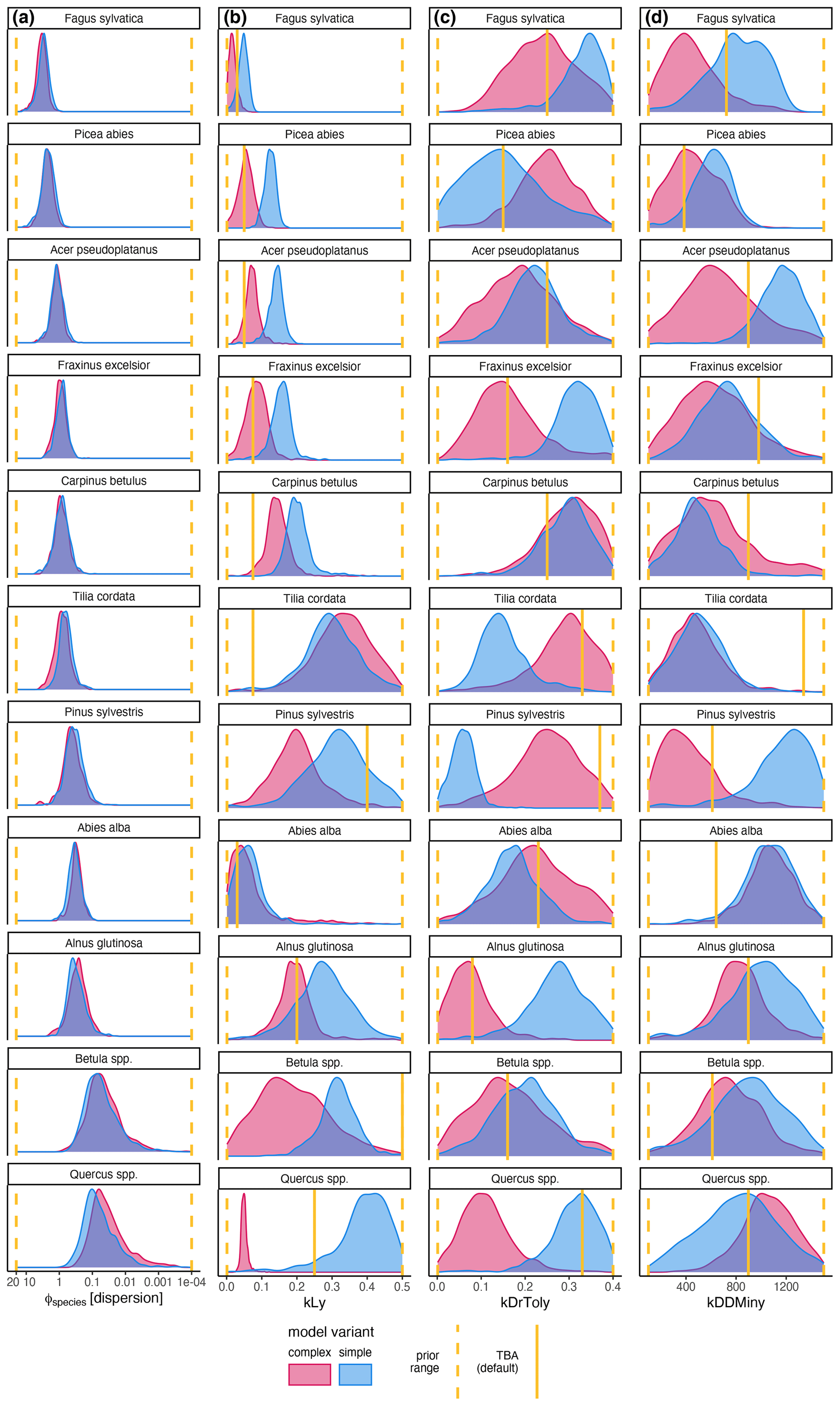
Figure A1Posterior distribution of species-specific parameters for the complex model (red) and the simple model (blue). Column (a) shows the species-specific dispersion parameter ϕ. The other columns show the ecological regeneration thresholds: (b) shows the light requirements (kLy), (c) shows the drought tolerance (kDrToly), and (d) shows the degree-days (kDDMiny). The species are sorted row-wise according to their average dispersions across both models. The prior parameter range and the expected value are indicated by the dashed and solid yellow lines, respectively.
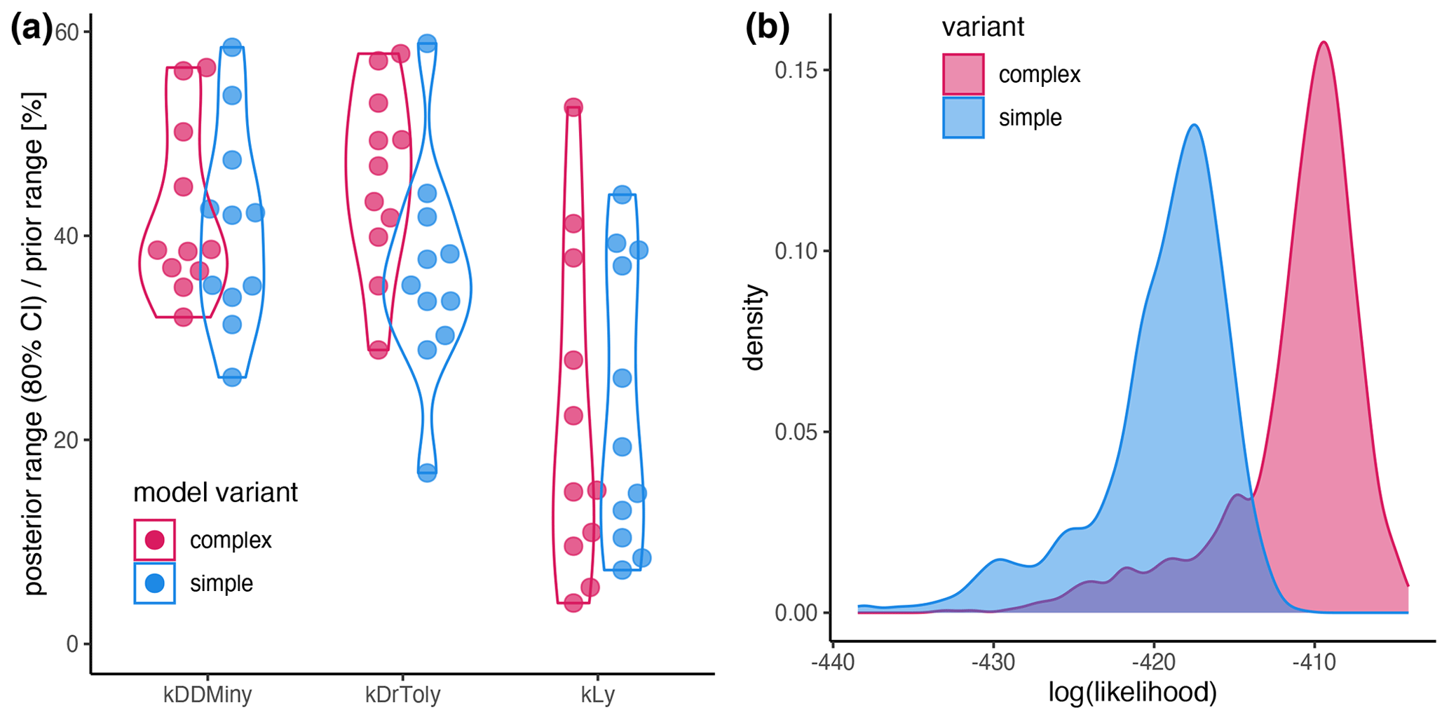
Figure A2(a) Sensitivity of the parameters expressed as the percentage of the prior range that is covered by the 80 % CI. (b) Likelihood distribution of the posterior simulations from the simple model (blue) and the complex model (red). The results for the complex model and the simple model are shown in red and blue, respectively.
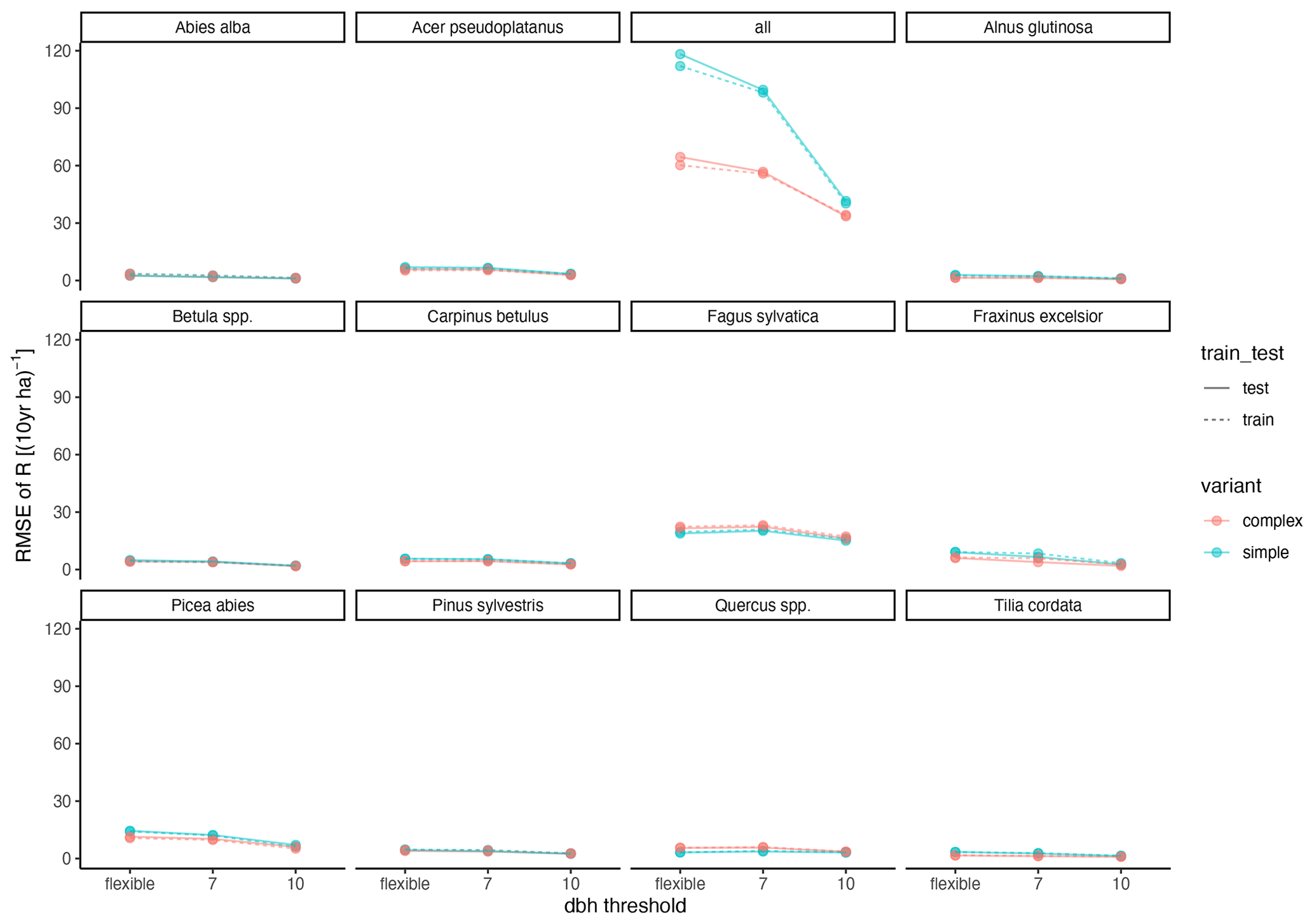
Figure A3Relationship between RMSE and DBH threshold. “flexible” refers to the individual DBH thresholds applied during model calibration. The DBH thresholds“7” and “10” refer to the subset of sites which had DBHs of at least 7 and 10 cm, respectively.
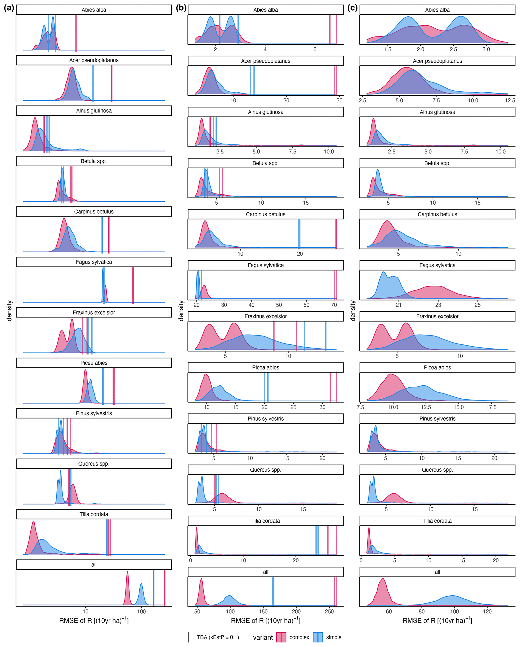
Figure A4RMSE of the difference between posterior predictions () and observations (R). Axis scaling: (a) log10 scaled; (b) the x-axis range varies with the RMSE of the trait-based approach (TBA; the default); the x-axis range varies between species with the RMSE of the inverse calibration (ICA).
Table A1Posterior values of the recruitment amount parameters kTrMax (complex model) and kEstDens (simple model), and the effects of DBH ϕDBH and plot area ϕA on dispersion. The outer values refer to the 80 % CIs and the middle values refer to the MPE (i.e., 10 %CI | MPE | 90 %CI).
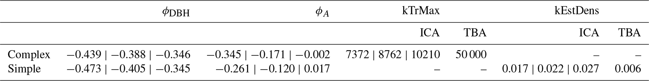
Table A2Species posterior parameter values for light requirements (kLy), drought tolerance (kDrToly), and degree-days (kDDMiny), including their default values. The outer values refer to the 80 % CIs and the middle values refer to the MPE (i.e., 10 %CI | MPE | 90 %CI). * Default values for Betula spp. are those of Betula pendula; default values for Quercus spp. are those of Quercus petraea.
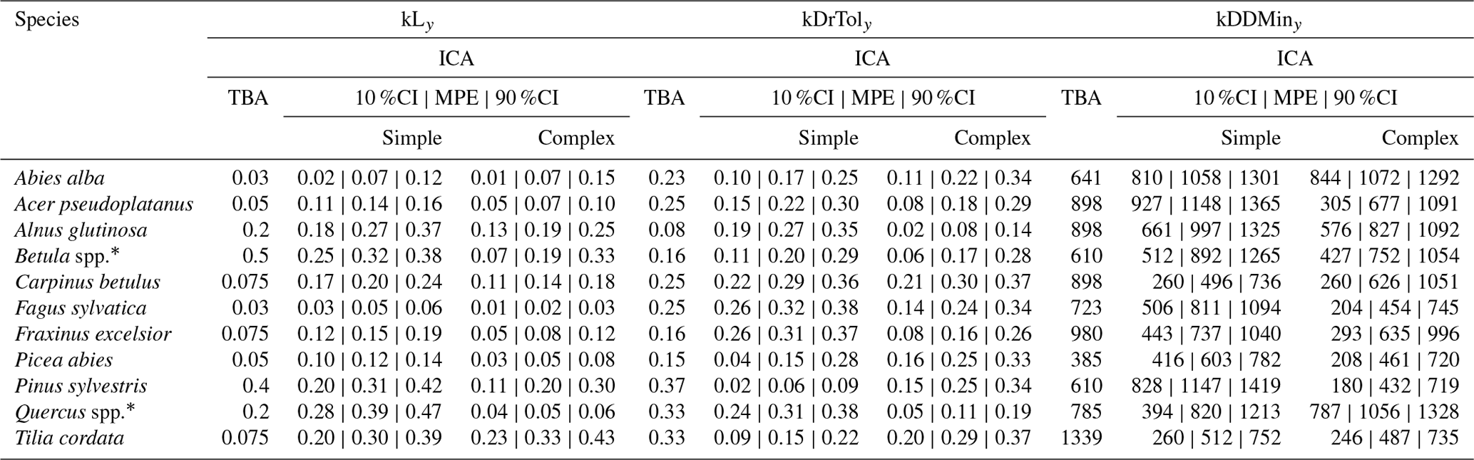
Table A3Species dispersion parameter posterior values. The outer values refer to the 80 % CIs and the middle values refer to the MPE (i.e., 10 %CI | MPE | 90 %CI).
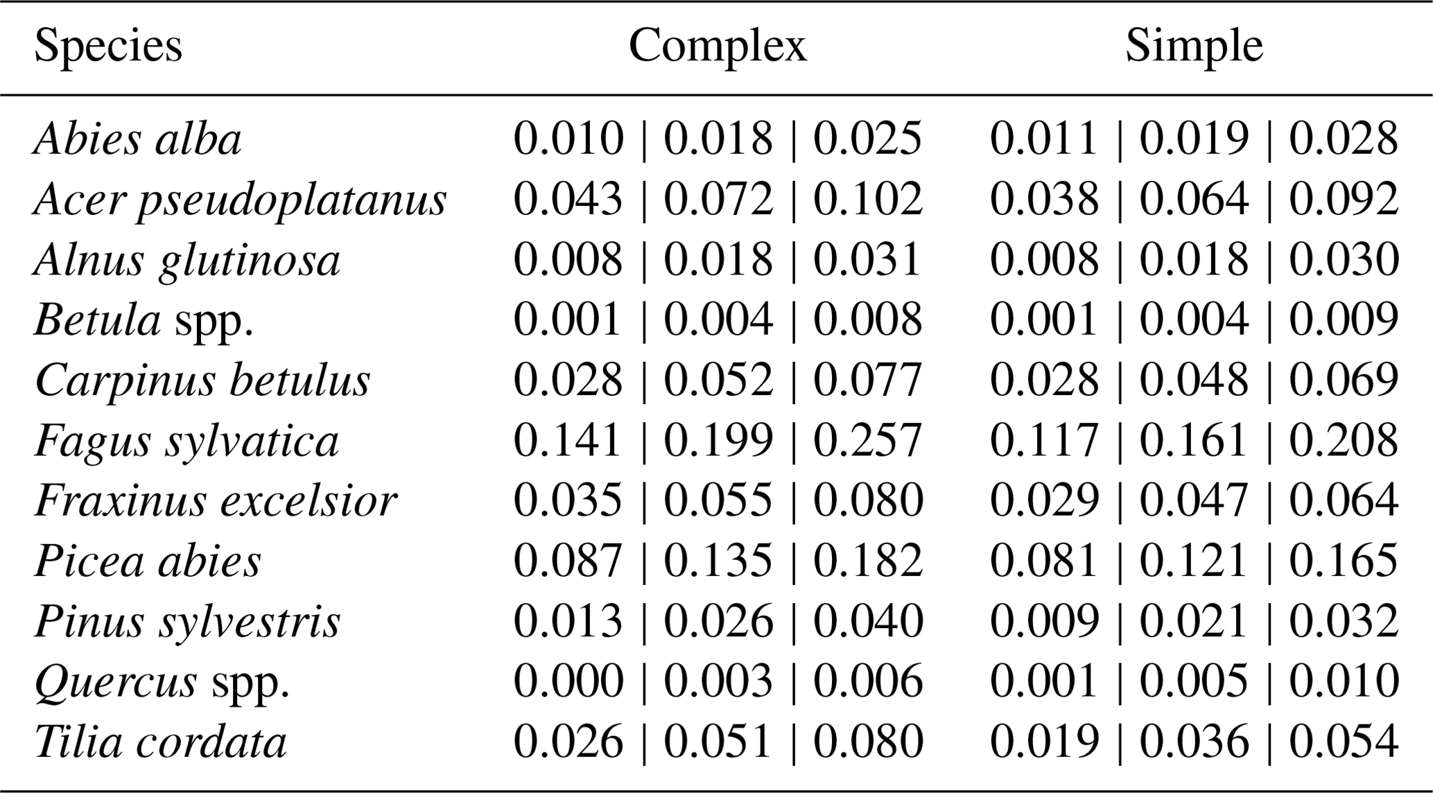
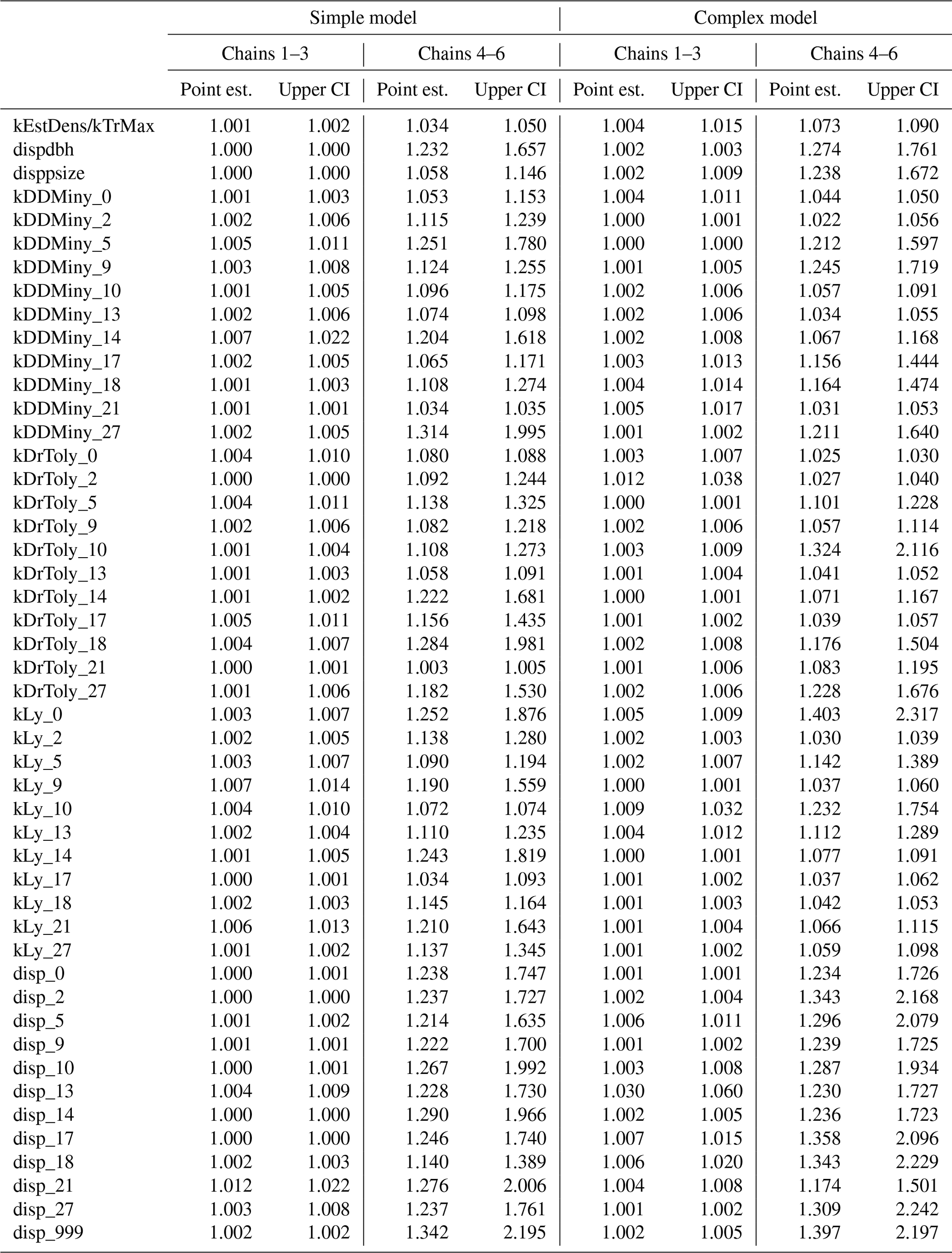
Table A4Gelman–Rubin diagnostics for the simple and complex models split into two sets of independent chains.
This appendix provides a detailed description of the two model variants used in this study. It complements the description in the main script (Fig. 1) but only covers the regeneration module of ForClim. Note that this model incorporates some minor changes compared to the original formulations in Bugmann (1994) for the simple model and Huber et al. (2020) for the complex model. However, these changes do not affect the functioning of the model.
B1 Step 1 – does regeneration take place?
The first step is to determine whether regeneration takes place at all in any given year; this is done for each species on each patch. The probability of regeneration (kEstP) was set to 2 % for the calibration – lower than the default value (10 %) of kEstP in the default model (the trait-based approach). This was done to reduce the number of cohorts and thus computational costs. The reduction, however, does not reduce the effective regeneration because it can be compensated for by the parameters for the regeneration amount (kEstDens and kTrMax; see Table B1 and Eqs. (B2) and (B3)) in the sense that reducing kEstP by a factor of 1/5, for example, can be compensated for by increasing kEstDens or kTrMax by a factor of 5.
where U is a function that draws a random number from a uniform distribution ranging from 0 to 1. The complex model determines whether regeneration takes place (PEst = 1) or not (PEst = 0) regardless of the species, but it does depend on the site factors degree-days (mDDAn) and drought (mDrAn). Specifically, PEst is calculated with
B2 Step 2 – how much regeneration?
Second, the number of new trees is calculated.
The simple model simulates the maximum regeneration amount per species based on the establishment intensity parameter (kEstDens) but also on kLas, which is used as a proxy for seed production (Huber et al., 2020; Risch et al., 2005). Specifically, the maximum regeneration kEstMaxs for species s is calculated with
where kPatchSize is the patch size, which was set to 800 m2 In the complex model, the regeneration amount is regulated by the continuous establishment flag (EFc) of the most suitable species, site factors (see the calculation of gRedFac in Eq. (B2)), and the regeneration intensity parameter kTrMax. Specifically, the regeneration amount over all species (nTrs) is calculated with
B3 Step 3 – what species?
Third, the final number of new trees for each species (nTrss) is determined.
In the simple model, for each species s, a random number between 1 and kEstMaxs is drawn, with
In the complex model, nTrss is calculated for each species s based on its suitability for regeneration (EFcs) and relative to the suitability of all other species (EFSum) with
Ultimately, nTrss denotes the number of trees with a DBH of 1.27 cm in a new cohort per species s on one patch, and it serves as a basis for calculating the likelihood (see below). After a new cohort has established, it follows the rules of adult growth and mortality, which are kept unchanged throughout this study by keeping all model parameters that directly affect trees with DBHs above 1.27 cm at their defaults (Bugmann, 1994; Huber et al., 2020).
Table B1Description of all model variables and parameters of ForClim used in this study. Calibrated parameters are explained in more detail in Table 1 in the main text.
The current version of ForClim is available from the project website: https://ites-fe.ethz.ch/openaccess/products/forclim (last access: 15 September 2023) under the GNU General Public License v3. The exact version of ForClim used to produce the results used in this paper is archived on Zenodo (https://doi.org/10.5281/zenodo.8334091, Käber et al., 2024), as are the input data and scripts used to run the model and produce the plots for all the simulations presented in this paper (https://doi.org/10.5281/zenodo.8334091, Käber et al., 2024).
YK, FH, and HB conceived the idea and developed the concept for this study; YK led the writing of the paper, conducted the analysis, and created the graphics. FH provided statistical support. HB secured funding. All authors contributed to writing the paper.
The contact author has declared that none of the authors has any competing interests.
Publisher's note: Copernicus Publications remains neutral with regard to jurisdictional claims made in the text, published maps, institutional affiliations, or any other geographical representation in this paper. While Copernicus Publications makes every effort to include appropriate place names, the final responsibility lies with the authors.
We thank all researchers of the European Forest Reserves Initiative (EuFoRIa, http://www.euforia-project.org, last access: 5 April 2023) who contributed long-term data to this study. EuFoRIa has been invaluable for this study, and we are grateful for its support and trust. In particular, we thank Thomas A. Nagel (University of Ljubljana, Ljubljana, Slovenia), Tuomas Aakala (University of Eastern Finland, Joensuu, Finland), Markus Blaschke (Bavarian State Institute for Forestry, Freising, Germany), Bogdan Brzeziecki (Warsaw University of Life Sciences, Warsaw, Poland), Marco Carrer (University of Padua, Legnaro, Italy), Eugenie Cateau (Reserves Naturelles de France, Quetigny, France), Georg Frank (Austrian Federal Research Centre for Forests, Natural Hazards and Landscape (BFW), Vienna, Austria), Shawn Fraver (School of Forest Resources, University of Maine, Orono, Maine, USA), Jan Holik (Silva Tarouca Research Institute, Brno, Czech Republic), Stanislav Kucbel (Department of Silviculture, Faculty of Forestry, Technical University in Zvolen, Slovakia), Anja Leyman (Research Institute for Nature and Forest, Brussels, Belgium), Peter Meyer (Northwest German Forest Research Institute, Göttingen, Germany), Renzo Motta (University of Turin, Turin, Italy), Pavel Samonil (Silva Tarouca Research Institute, Brno, Czech Republic), Lucia Seebach (Forest Research Institute of Baden-Württemberg, Freiburg, Germany), Jonas Stillhard (Swiss Federal Institute for Forest, Snow and Landscape Research, Birmensdorf, Switzerland), Miroslav Svoboda (Czech University of Life Sciences, Prague, Czech Republic), Jerzy Szwagrzyk (University of Agriculture, Kraków, Poland), Kris Vandekerkhove (Research Institute for Nature and Forest, Brussels, Belgium), Ondrej Vostarek (Czech University of Life Sciences, Prague, Czech Republic), Kamil Kral (Czech University of Life Sciences, Prague, Czech Republic), and Tzvetan Zlatanov (Institute of Biodiversity and Ecosystem Research, Bulgarian Academy of Sciences, Sofia, Bulgaria). In addition, we thank Hussain Abbas, who provided programming support and facilitated the use of the Euler HPC cluster.
This study is part of Yannek Käber's PhD project and was funded by ETH Zurich (grant no. ETH-35 18-1).
This paper was edited by Hisashi Sato and reviewed by two anonymous referees.
Andivia, E., Madrigal-González, J., Villar-Salvador, P., and Zavala, M. A.: Do adult trees increase conspecific juvenile resilience to recurrent droughts? Implications for forest regeneration, Ecosphere, 9, e02282, https://doi.org/10.1002/ecs2.2282, 2018.
Augustynczik, A. L. D., Hartig, F., Minunno, F., Kahle, H.-P., Diaconu, D., Hanewinkel, M., and Yousefpour, R.: Productivity of Fagus sylvatica under climate change – A Bayesian analysis of risk and uncertainty using the model 3-PG, Forest Ecol. Manag., 401, 192–206, https://doi.org/10.1016/J.FORECO.2017.06.061, 2017.
Botkin, D. B., Janak, J. F., and Wallis, J. R.: Some Ecological Consequences of a Computer Model of Forest Growth, J. Ecol., 60, 849–849, https://doi.org/10.2307/2258570, 1972.
Bröcker, J. and Smith, L. A.: Scoring Probabilistic Forecasts: The Importance of Being Proper, Weather Forecast., 22, 382–388, https://doi.org/10.1175/WAF966.1, 2007.
Brooks, M. E., Kristensen, K., Benthem, K. J. van, Magnusson, A., Berg, C. W., Nielsen, A., Skaug, H. J., Maechler, M., and Bolker, B. M.: glmmTMB Balances Speed and Flexibility Among Packages for Zero-inflated Generalized Linear Mixed Modeling, R J., 9, 378–400, 2017.
Bugmann, H.: On the ecology of mountainous forests in a changing climate: a simulation study, PhD Thesis, https://doi.org/10.3929/ethz-a-000946508, 1994.
Bugmann, H.: A Simplified Forest Model to Study Species Composition Along Climate Gradients, Ecology, 77, 2055–2074, https://doi.org/10.2307/2265700, 1996.
Bugmann, H. and Cramer, W.: Improving the behaviour of forest gap models along drought gradients, Forest Ecol. Manag., 103, 247–263, https://doi.org/10.1016/S0378-1127(97)00217-X, 1998.
Bugmann, H. and Seidl, R.: The evolution, complexity and diversity of models of long-term forest dynamics, J. Ecol., 110, 2288–2307, https://doi.org/10.1111/1365-2745.13989, 2022.
Bugmann, H. and Solomon, A. M.: Explaining Forest Composition and Biomass Across Multiple Biogeographical Regions, Ecol. Appl., 10, 95–114, https://doi.org/10.1890/1051-0761(2000)010[0095:EFCABA]2.0.CO;2, 2000.
Cailleret, M., Bircher, N., Hartig, F., Hülsmann, L., and Bugmann, H.: Bayesian calibration of a growth‐dependent tree mortality model to simulate the dynamics of European temperate forests, Ecol. Appl., 30, e02021, https://doi.org/10.1002/eap.2021, 2019.
Chalmandrier, L., Hartig, F., Laughlin, D. C., Lischke, H., Pichler, M., Stouffer, D. B., and Pellissier, L.: Linking functional traits and demography to model species-rich communities, Nat. Commun., 12, 2724, https://doi.org/10.1038/s41467-021-22630-1, 2021.
Clark, J. S., Beckage, B., Camill, P., Cleveland, B., HilleRisLambers, J., Lichter, J., McLachlan, J., Mohan, J., and Wyckoff, P.: Interpreting recruitment limitation in forests, Am. J. Bot., 86, 1–16, https://doi.org/10.2307/2656950, 1999.
Clark, J. S., Iverson, L., Woodall, C. W., Allen, C. D., Bell, D. M., Bragg, D. C., D'Amato, A. W., Davis, F. W., Hersh, M. H., Ibanez, I., Jackson, S. T., Matthews, S., Pederson, N., Peters, M., Schwartz, M. W., Waring, K. M., and Zimmermann, N. E.: The impacts of increasing drought on forest dynamics, structure, and biodiversity in the United States, Glob. Change Biol., 22, 2329–2352, https://doi.org/10.1111/gcb.13160, 2016.
Collins, S. L. and Good, R. E.: The Seedling Regeneration Niche: Habitat Structure of Tree Seedlings in an Oak-Pine Forest, Oikos, 48, 89–98, https://doi.org/10.2307/3565692, 1987.
Csilléry, K., Blum, M. G. B., Gaggiotti, O. E., and François, O.: Approximate Bayesian Computation (ABC) in practice, Trends Ecol. Amp Evol., 25, 410–418, https://doi.org/10.1016/J.TREE.2010.04.001, 2010.
Delpierre, N., Lireux, S., Hartig, F., Camarero, J. J., Cheaib, A., Èufar, K., Cuny, H., Deslauriers, A., Fonti, P., Grièar, J., Huang, J.-G., Krause, C., Liu, G., de Luis, M., Mäkinen, H., del Castillo, E. M., Morin, H., Nöjd, P., Oberhuber, W., Prislan, P., Rossi, S., Saderi, S. M., Treml, V., Vavrick, H., and Rathgeber, C. B. K.: Chilling and forcing temperatures interact to predict the onset of wood formation in Northern Hemisphere conifers, Glob. Change Biol., 25, 1089–1105, https://doi.org/10.1111/gcb.14539, 2019.
Detto, M., Levine, J. M., and Pacala, S. W.: Maintenance of high diversity in mechanistic forest dynamics models of competition for light, Ecol. Monogr., 92, e1500, https://doi.org/10.1002/ecm.1500, 2022.
Díaz-Yáñez, O., Käber, Y., Anders, T., Bohn, F., Braziunas, K. H., Brůna, J., Fischer, R., Fischer, S. M., Hetzer, J., Hickler, T., Hochauer, C., Lexer, M. J., Lischke, H., Mairota, P., Merganič, J., Merganičová, K., Mette, T., Mina, M., Morin, X., Nieberg, M., Rammer, W., Reyer, C. P. O., Scheiter, S., Scherrer, D., and Bugmann, H.: Tree regeneration in models of forest dynamics: A key priority for further research, Ecosphere, 15, e4807, https://doi.org/10.1002/ecs2.4807, 2024.
Didion, M., Kupferschmid, A. D., Zingg, A., Fahse, L., and Bugmann, H.: Gaining local accuracy while not losing generality – extending the range of gap model applications, Can. J. Forest Res., 39, 1092–1107, https://doi.org/10.1139/X09-041, 2009a.
Didion, M., Kupferschmid, A. D., and Bugmann, H.: Long-term effects of ungulate browsing on forest composition and structure, Forest Ecol. Manag., https://doi.org/10.1016/j.foreco.2009.06.006, 2009b.
Dietze, M. C.: Ecological Forecasting, Princeton University Press, https://doi.org/10.2307/j.ctvc7796h, 2017.
Ellenberg, H.: Vegetation Mitteleuropas mit den Alpen in ökologischer Sicht, 4th Edn., Ulmer, Stuttgart Germany, 989 pp., ISBN 9783800134304, 1986.
Ellenberg, H. and Klötzli, F.: Waldgesellschaften und waldstandorte der schweiz, Eidgenössische Anstalt f. d. Forstl. Versuchswesen, https://www.dora.lib4ri.ch/wsl/islandora/object/wsl:13641 (last access: 9 April 2024), 1972.
Grant, K., Kreyling, J., Heilmeier, H., Beierkuhnlein, C., and Jentsch, A.: Extreme weather events and plant–plant interactions: shifts between competition and facilitation among grassland species in the face of drought and heavy rainfall, Ecol. Res., 29, 991–1001, https://doi.org/10.1007/s11284-014-1187-5, 2014.
Grime, J. P.: Evidence for the Existence of Three Primary Strategies in Plants and Its Relevance to Ecological and Evolutionary Theory, Am. Nat., 111, 1169–1194, https://doi.org/10.1086/283244, 1977.
Grime, J. P. and Mackey, J. M. L.: The role of plasticity in resource capture by plants, Evol. Ecol., 16, 299–307, https://doi.org/10.1023/A:1019640813676, 2002.
Grossiord, C.: Having the right neighbors: how tree species diversity modulates drought impacts on forests, New Phytol., 228, 42–49, https://doi.org/10.1111/nph.15667, 2020.
Grubb, P. J.: The maintenance of species-richness in plant communities: The importance of the regeneration niche, Biol. Rev., 52, 107–145, https://doi.org/10.1111/j.1469-185X.1977.tb01347.x, 1977.
Haberstroh, S. and Werner, C.: The role of species interactions for forest resilience to drought, Plant Biol., 24, 1098–1107, https://doi.org/10.1111/plb.13415, 2022.
Hanbury-Brown, A. R., Ward, R. E., and Kueppers, L. M.: Forest regeneration within Earth system models: current process representations and ways forward, New Phytol., 235, 20–40, https://doi.org/10.1111/nph.18131, 2022.
Hart, S. P., Usinowicz, J., and Levine, J. M.: The spatial scales of species coexistence, Nat. Ecol. Evol., 1, 1066–1073, https://doi.org/10.1038/s41559-017-0230-7, 2017.
Hartig, F., Calabrese, J. M., Reineking, B., Wiegand, T., and Huth, A.: Statistical inference for stochastic simulation models – theory and application, Ecol. Lett., 14, 816–827, https://doi.org/10.1111/j.1461-0248.2011.01640.x, 2011.
Hartig, F., Dyke, J., Hickler, T., Higgins, S. I., O'Hara, R. B., Scheiter, S., and Huth, A.: Connecting dynamic vegetation models to data – an inverse perspective, J. Biogeogr., 39, 2240–2252, https://doi.org/10.1111/j.1365-2699.2012.02745.x, 2012.
Hartig, F., Minunno, F., and Paul, S.: BayesianTools: General-Purpose MCMC and SMC Samplers and Tools for Bayesian Statistics, https://cran.r-project.org/package=BayesianTools (last access: 9 April 2024), 2019.
Heiland, L., Kunstler, G., Ruiz-Benito, P., Buras, A., Dahlgren, J., and Hülsmann, L.: Divergent occurrences of juvenile and adult trees are explained by both environmental change and ontogenetic effects, Ecography, 2022, e06042, https://doi.org/10.1111/ecog.06042, 2022.
Hellegers, M., Ozinga, W. A., Hinsberg van, A., Huijbregts, M. A. J., Hennekens, S. M., Schaminée, J. H. J., Dengler, J., and Schipper, A. M.: Evaluating the ecological realism of plant species distribution models with ecological indicator values, Ecography, 43, 161–170, https://doi.org/10.1111/ecog.04291, 2020.
Huber, N., Bugmann, H., and Lafond, V.: Global sensitivity analysis of a dynamic vegetation model: Model sensitivity depends on successional time, climate and competitive interactions, Ecol. Model., 368, 377–390, https://doi.org/10.1016/J.ECOLMODEL.2017.12.013, 2018.
Huber, N., Bugmann, H., and Lafond, V.: Capturing ecological processes in dynamic forest models: why there is no silver bullet to cope with complexity, Ecosphere, 11, e03109, https://doi.org/10.1002/ecs2.3109, 2020.
Jucker, T., Bouriaud, O., Avacaritei, D., Dãnilã, I., Duduman, G., Valladares, F., and Coomes, D. A.: Competition for light and water play contrasting roles in driving diversity–productivity relationships in Iberian forests, J. Ecol., 102, 1202–1213, https://doi.org/10.1111/1365-2745.12276, 2014.
Käber, Y., Meyer, P., Stillhard, J., Lombaerde, E. D., Zell, J., Stadelmann, G., Bugmann, H., and Bigler, C.: Tree recruitment is determined by stand structure and shade tolerance with uncertain role of climate and water relations, Ecol. Evol., 11, 12182–12203, https://doi.org/10.1002/ece3.7984, 2021.
Käber, Y., Bigler, C., HilleRisLambers, J., Hobi, M., Nagel, T. A., Aakala, T., Blaschke, M., Brang, P., Brzeziecki, B., Carrer, M., Cateau, E., Frank, G., Fraver, S., Idoate-Lacasia, J., Holik, J., Kucbel, S., Leyman, A., Meyer, P., Motta, R., Samonil, P., Seebach, L., Stillhard, J., Svoboda, M., Szwagrzyk, J., Vandekerkhove, K., Vostarek, O., Zlatanov, T., and Bugmann, H.: Sheltered or suppressed? Tree regeneration in unmanaged European forests, J. Ecol., 111, 2281–2295, https://doi.org/10.1111/1365-2745.14181, 2023.
Käber, Y., Hartig, F., and Bugmann, H.: Supplementary material for Käber et al. “Inferring the regeneration niche from forest inventory data using a dynamic forest model”. In Geoscientific Model Development (2.0), Zenodo [code and data set], https://doi.org/10.5281/zenodo.8334091, 2024.
Karger, D. N., Conrad, O., Böhner, J., Kawohl, T., Kreft, H., Soria-Auza, R. W., Zimmermann, N. E., Linder, H. P., and Kessler, M.: Climatologies at high resolution for the earth’s land surface areas, Sci. Data, 4, 170122–170122, https://doi.org/10.1038/sdata.2017.122, 2017.
Kass, R. E. and Raftery, A. E.: Bayes Factors, J. Am. Stat. Assoc., 90, 773–795, https://doi.org/10.1080/01621459.1995.10476572, 1995.
Kienast, F.: FORECE: A forest succession model for southern Central Europe, United States, https://www.osti.gov/biblio/5729437 (last access: 9 April 2024), 1987.
Köhler, P. and Huth, A.: The effects of tree species grouping in tropical rainforest modelling: Simulations with the individual-based model Formind, Ecol. Model., 109, 301–321, https://doi.org/10.1016/S0304-3800(98)00066-0, 1998.
König, L. A., Mohren, F., Schelhaas, M.-J., Bugmann, H., and Nabuurs, G.-J.: Tree regeneration in models of forest dynamics – Suitability to assess climate change impacts on European forests, Forest Ecol. Manag., 520, 120390, https://doi.org/10.1016/j.foreco.2022.120390, 2022.
Larcher, W.: Physiological plant ecology, Acta Physiol. Plant., 18, 183–184, 1996.
Lett, S. and Dorrepaal, E.: Global drivers of tree seedling establishment at alpine treelines in a changing climate, Funct. Ecol., 32, 1666–1680, https://doi.org/10.1111/1365-2435.13137, 2018.
Leuschner, C. and Ellenberg, H.: Ecology of Central European Forests: Vegetation Ecology of Central Europe, Volume I, Springer International Publishing, Cham, https://doi.org/10.1007/978-3-319-43042-3, 2017.
Levine, J. I., Levine, J. M., Gibbs, T., and Pacala, S. W.: Competition for water and species coexistence in phenologically structured annual plant communities, Ecol. Lett., 25, 1110–1125, https://doi.org/10.1111/ele.13990, 2022.
Li, Y., Jiang, Y., Zhao, K., Chen, Y., Wei, W., Shipley, B., and Chu, C.: Exploring trait–performance relationships of tree seedlings along experimentally manipulated light and water gradients, Ecology, 103, e3703, https://doi.org/10.1002/ecy.3703, 2022.
Lortie, C. J. and Callaway, R. M.: Re-analysis of meta-analysis: support for the stress-gradient hypothesis, J. Ecol., 94, 7–16, https://doi.org/10.1111/j.1365-2745.2005.01066.x, 2006.
Lyr, H. (Ed.): Physiologie und Ökologie der Gehölze, Fischer, Jena Stuttgart, 620 pp., ISBN 9783334003978, 1992.
Mauri, A., Girardello, M., Strona, G., Beck, P. S. A., Forzieri, G., Caudullo, G., Manca, F., and Cescatti, A.: EU-Trees4F, a dataset on the future distribution of European tree species, Sci. Data, 9, 37, https://doi.org/10.1038/s41597-022-01128-5, 2022.
McDowell, N. G., Allen, C. D., Anderson-Teixeira, K., Aukema, B. H., Bond-Lamberty, B., Chini, L., Clark, J. S., Dietze, M., Grossiord, C., Hanbury-Brown, A., Hurtt, G. C., Jackson, R. B., Johnson, D. J., Kueppers, L., Lichstein, J. W., Ogle, K., Poulter, B., Pugh, T. A. M., Seidl, R., Turner, M. G., Uriarte, M., Walker, A. P., and Xu, C.: Pervasive shifts in forest dynamics in a changing world, Science, 368, eaaz9463, https://doi.org/10.1126/science.aaz9463, 2020.
Meusel, H., Jäger, E., and Weinert, E.: Vergleichende Chorologie der zentraleuropäischen Flora – Band 1, G. Fischer Verlag, 1965.
Morin, X. and Thuiller, W.: Comparing niche- and process-based models to reduce prediction uncertainty in species range shifts under climate change, Ecology, 90, 1301–1313, https://doi.org/10.1890/08-0134.1, 2009.
Müller, M. J.: Selected climatic data for a global set of standard stations for vegetation science, Springer Netherlands, Dordrecht, https://doi.org/10.1007/978-94-009-8040-2, 1982.
Oberpriller, J., Cameron, D. R., Dietze, M. C., and Hartig, F.: Towards robust statistical inference for complex computer models, Ecol. Lett., 24, 1251–1261, https://doi.org/10.1111/ele.13728, 2021.
O'Hagan, A.: Fractional Bayes Factors for Model Comparison, J. Roy. Stat. Soc. Ser. B, 57, 99–118, https://doi.org/10.1111/j.2517-6161.1995.tb02017.x, 1995.
Paine, C. E. T., Amissah, L., Auge, H., Baraloto, C., Baruffol, M., Bourland, N., Bruelheide, H., Daïnou, K., Gouvenain, R. C. de, Doucet, J.-L., Doust, S., Fine, P. V. A., Fortunel, C., Haase, J., Holl, K. D., Jactel, H., Li, X., Kitajima, K., Koricheva, J., Martínez-Garza, C., Messier, C., Paquette, A., Philipson, C., Piotto, D., Poorter, L., Posada, J. M., Potvin, C., Rainio, K., Russo, S. E., Ruiz-Jaen, M., Scherer-Lorenzen, M., Webb, C. O., Wright, S. J., Zahawi, R. A., and Hector, A.: Globally, functional traits are weak predictors of juvenile tree growth, and we do not know why, J. Ecol., 103, 978–989, https://doi.org/10.1111/1365-2745.12401, 2015.
Price, D. T., Zimmermann, N. E., van der Meer, P. J., Lexer, M. J., Leadley, P., Jorritsma, I. T. M., Schaber, J., Clark, D. F., Lasch, P., McNulty, S., Wu, J., and Smith, B.: Regeneration in Gap Models: Priority Issues for Studying Forest Responses to Climate Change, Clim. Change, 51, 475–508, https://doi.org/10.1023/A:1012579107129, 2001.
QGIS Development Team: QGIS Geographic Information System, QGIS Association, 2022.
Risch, A. C., Heiri, C., and Bugmann, H.: Simulating structural forest patterns with a forest gap model: a model evaluation, Ecol. Model., 181, 161–172, https://doi.org/10.1016/j.ecolmodel.2004.06.029, 2005.
Rudloff, W.: World climates, Wissenschaftliche Verlagsgesellschaft, Stuttgart, ISBN 380470509X, 1981.
Rüger, N., Huth, A., Hubbell, S. P., and Condit, R.: Response of recruitment to light availability across a tropical lowland rain forest community, J. Ecol., 97, 1360–1368, https://doi.org/10.1111/j.1365-2745.2009.01552.x, 2009.
Ruiz-Benito, P., Lines, E. R., Gómez-Aparicio, L., Zavala, M. A., and Coomes, D. A.: Patterns and Drivers of Tree Mortality in Iberian Forests: Climatic Effects Are Modified by Competition, PLOS ONE, 8, e56843, https://doi.org/10.1371/journal.pone.0056843, 2013.
Scherrer, D., Vitasse, Y., Guisan, A., Wohlgemuth, T., and Lischke, H.: Competition and demography rather than dispersal limitation slow down upward shifts of trees' upper elevation limits in the Alps, J. Ecol., 108, 2416–2430, https://doi.org/10.1111/1365-2745.13451, 2020.
Seidl, R. and Turner, M. G.: Post-disturbance reorganization of forest ecosystems in a changing world, P. Natl. Acad. Sci. USA, 119, e2202190119, https://doi.org/10.1073/pnas.2202190119, 2022.
Seidl, R., Rammer, W., Scheller, R. M., and Spies, T. A.: An individual-based process model to simulate landscape-scale forest ecosystem dynamics, Ecol. Model., 231, 87–100, https://doi.org/10.1016/J.ECOLMODEL.2012.02.015, 2012.
Shoemaker, L. G., Sullivan, L. L., Donohue, I., Cabral, J. S., Williams, R. J., Mayfield, M. M., Chase, J. M., Chu, C., Harpole, W. S., Huth, A., HilleRisLambers, J., James, A. R. M., Kraft, N. J. B., May, F., Muthukrishnan, R., Satterlee, S., Taubert, F., Wang, X., Wiegand, T., Yang, Q., and Abbott, K. C.: Integrating the underlying structure of stochasticity into community ecology, Ecology, 101, e02922, https://doi.org/10.1002/ecy.2922, 2020.
Shugart, H. H.: A theory of forest dynamics: the ecological implications of forest succession models, Springer-Verlag, New York, 278 pp., ISBN 9780387960005, 1984.
Smith, P., Beven, K. J., and Tawn, J. A.: Informal likelihood measures in model assessment: Theoretic development and investigation, Adv. Water Resour., 31, 1087–1100, https://doi.org/10.1016/j.advwatres.2008.04.012, 2008.
Svenning, J.-C., Normand, S., and Skov, F.: Postglacial dispersal limitation of widespread forest plant species in nemoral Europe, Ecography, 31, 316–326, https://doi.org/10.1111/j.0906-7590.2008.05206.x, 2008.
ter Braak, C. J. F. and Vrugt, J. A.: Differential Evolution Markov Chain with snooker updater and fewer chains, Stat. Comput., 18, 435–446, https://doi.org/10.1007/s11222-008-9104-9, 2008.
Thakur, M. P. and Wright, A. J.: Environmental Filtering, Niche Construction, and Trait Variability: The Missing Discussion, Trends Ecol. Evol., 32, 884–886, https://doi.org/10.1016/j.tree.2017.09.014, 2017.
Trotsiuk, V., Hartig, F., Cailleret, M., Babst, F., Forrester, D. I., Baltensweiler, A., Buchmann, N., Bugmann, H., Gessler, A., Gharun, M., Minunno, F., Rigling, A., Rohner, B., Stillhard, J., Thuerig, E., Waldner, P., Ferretti, M., Eugster, W., and Schaub, M.: Assessing the response of forest productivity to climate extremes in Switzerland using model-data fusion, Glob. Change Biol., 26, 2463–2476, https://doi.org/10.1111/gcb.15011, 2020.
Van Oijen, M., Rougier, J., and Smith, R.: Bayesian calibration of process-based forest models: bridging the gap between models and data, Tree Physiol., 25, 915–927, https://doi.org/10.1093/treephys/25.7.915, 2005.
Vincent, G. and Harja, D.: Exploring Ecological Significance of Tree Crown Plasticity through Three-dimensional Modelling, Ann. Bot., 101, 1221–1231, https://doi.org/10.1093/aob/mcm189, 2008.
Vitasse, Y.: Ontogenic changes rather than difference in temperature cause understory trees to leaf out earlier, New Phytol., 198, 149–155, https://doi.org/10.1111/nph.12130, 2013.
Welden, C. W. and Slauson, W. L.: The Intensity of Competition Versus its Importance: An Overlooked Distinction and Some Implications, Q. Rev. Biol., 61, 23–44, https://doi.org/10.1086/414724, 1986.
Werner, E. E. and Gilliam, J. F.: The Ontogenetic Niche and Species Interactions in Size-Structured Populations, Annu. Rev. Ecol. Syst., 15, 393–425, https://doi.org/10.1146/annurev.es.15.110184.002141, 1984.
Wood, S. N.: Statistical inference for noisy nonlinear ecological dynamic systems, Nature, 466, 1102–1104, https://doi.org/10.1038/nature09319, 2010.
Yang, J., Cao, M., and Swenson, N. G.: Why Functional Traits Do Not Predict Tree Demographic Rates, Trends Ecol. Evol., 33, 326–336, https://doi.org/10.1016/j.tree.2018.03.003, 2018.
Young, D. J. N., Stevens, J. T., Earles, J. M., Moore, J., Ellis, A., Jirka, A. L., and Latimer, A. M.: Long-term climate and competition explain forest mortality patterns under extreme drought, Ecol. Lett., 20, 78–86, https://doi.org/10.1111/ele.12711, 2017.
Zell, J., Rohner, B., Thürig, E., and Stadelmann, G.: Modeling ingrowth for empirical forest prediction systems, Forest Ecol. Manag., 433, 771–779, https://doi.org/10.1016/j.foreco.2018.11.052, 2019.