Implementing a dynamic representation of fire and harvest including subgrid-scale heterogeneity in the tile-based land surface model CLASSIC v1.45

Canada's forests play a critical role in the global carbon (C) cycle and are responding to unprecedented climate change as well as ongoing natural and anthropogenic disturbances. However, the representation of disturbance in boreal regions is limited in pre-existing land surface models (LSMs). Moreover, many LSMs do not explicitly represent subgrid-scale heterogeneity resulting from disturbance. To address these limitations, we implement harvest and wildfire forcings in the Canadian Land Surface Scheme Including Biogeochemical Cycles (CLASSIC) land surface model alongside dynamic tiling that represents subgrid-scale heterogeneity due to disturbance. The disturbances are captured using 30 m spatial resolution satellite data (Landsat) on an annual basis for 33 years. Using the pan-Canadian domain (i.e., all of Canada south of 76° N) as our study area for demonstration, we determine the model setup that optimally balances a detailed process representation and computational efficiency. We then demonstrate the impacts of subgrid-scale heterogeneity relative to standard average individual-based representations of disturbance and explore the resultant differences between the simulations. Our results indicate that the modeling approach implemented can balance model complexity and computational cost to represent the impacts of subgrid-scale heterogeneity resulting from disturbance. Subgrid-scale heterogeneity is shown to have impacts 1.5 to 4 times the impact of disturbance alone on gross primary productivity, autotrophic respiration, and surface energy balance processes in our simulations. These impacts are a result of subgrid-scale heterogeneity slowing vegetation re-growth and affecting surface energy balance in recently disturbed, sparsely vegetated, and often snow-covered fractions of the land surface. Representing subgrid-scale heterogeneity is key to more accurately representing timber harvest, which preferentially impacts larger trees on higher quality and more accessible sites. Our results show how different discretization schemes can impact model biases resulting from the representation of disturbance. These insights, along with our implementation of dynamic tiling, may apply to other tile-based LSMs. Ultimately, our results enhance our understanding of, and ability to represent, disturbance within Canada, facilitating a comprehensive process-based assessment of Canada's terrestrial C cycle.

1 Introduction

Canada's forests play a critical role in the global carbon (C) cycle (Keenan and Williams, 2018; Lenton et al., 2008). Canada's forests are also responding to both unprecedented climate change and ongoing anthropogenic disturbance (Lenton et al., 2008; White et al., 2017). Unfortunately, disentangling the relative impacts of disturbance processes and climate change on the Canadian forest C cycle is difficult (Sulla-Menashe et al., 2018; Goetz et al., 2005; Ju and Masek, 2016; Weber and Flannigan, 1997). Process-based land surface models (LSMs) provide a tool to evaluate the impacts of both types of disturbance, but there has only been limited representation of anthropogenic disturbance in regional or global C cycling assessments (Friedlingstein et al., 2019; Peng et al., 2014; Chaste et al., 2017; Hayes et al., 2012). Moreover, of those LSMs that do explicitly represent anthropogenic disturbance, only a small subset account for the resulting subgrid-scale heterogeneity (Le Quéré et al., 2018; Nabel et al., 2020; Pongratz et al., 2018). Here we demonstrate the impacts of disturbance and subgrid-scale heterogeneity on C and energy fluxes by implementing a dynamic tiling scheme in the Canadian Land Surface Scheme Including Biogeochemical Cycles (CLASSIC).

Subgrid-scale landscape heterogeneity refers to any characteristic of the landscape that differs at scales below that of the main model grid – in this case, differences in tree age and biomass in the burned or harvested subfraction of the grid cell. Tile-based LSMs, unlike individual-based models (i.e., models which simulate the landscape using several heterogeneous individuals), do not inherently represent subgrid-scale heterogeneity. Instead, the tile represents the average individual of a given plant function type (PFT) and thus represents the PFT's average state within the grid cell (a single height, biomass, etc.), which is used to simulate fluxes. Although most tile-based LSMs account for wood harvest, few represent the resulting subgrid-scale landscape heterogeneity, instead representing the impact of disturbances on the average individual PFT (Le Quéré et al., 2018; Pongratz et al., 2018; Nabel et al., 2020).

Stand-replacing forest disturbances (i.e., timber harvest and fire) directly impact forest C stocks through the removal of standing biomass (Wulder et al., 2020). In addition, stand-replacing disturbances also impact stand structure, especially in the case of managed timber harvest (Pan et al., 2010; Kuuluvainen and Gauthier, 2018; Pan et al., 2013). The resulting stand structure impacts forest function such as the exchange of matter and energy with the atmosphere as well as the forest's response to climate change (Erb et al., 2017; Luyssaert et al., 2014; Körner, 2006; Dore et al., 2010; Liu, 2005; Maness et al., 2012; Hirano et al., 2017). Historically, 0.4 % of Canada's ∼ 650 Mh of forested ecosystems are affected by stand-replacing disturbance per year (White et al., 2017). The age structure of Canadian forests due to historical disturbance has impacted the strength of the historical C sink in Canadian forests (Kurz and Apps, 1999, 1993; Böttcher et al., 2008). The age structure resulting from disturbance also influences the surface energy balance of stands by, for example, altering the sensible heat flux due to differences in snow cover and albedo and altering the seasonality of surface energy budgets and land surface properties (Liu, 2005; Maness et al., 2012). Therefore, it is key that we enhance our ability to accurately represent both disturbance processes and the influence of the subgrid-scale heterogeneity that disturbances produce within LSMs.

Disturbance events impact the response of Canada's forests to climate change. The responses of forest productivity, forest soil decomposition processes, and evaporation rates to warming, rising CO₂ concentrations, and changes to precipitation regimes will depend on stand structural characteristics and tree species characteristics (Hember et al., 2012; Kurz et al., 1997; Körner, 2006; Shrestha and Chen, 2010; Bond-Lamberty and Gower, 2008; Czimczik et al., 2006; Kurz et al., 2008). Warmer temperatures and higher atmospheric CO₂ concentrations are likely to increase the productivity of boreal forests, whereas drought stress and changing disturbance regimes are likely to decrease productivity and enhance the decomposition of soil C, leading to a patchwork of contrasting future responses (Babst et al., 2019; Reich et al., 2018; Lenton et al., 2008; Weber and Flannigan, 1997; Potapov et al., 2008; Ju and Chen, 2008; Sulla-Menashe et al., 2018). Complex changes in vegetation productivity have already been observed across the pan-Canadian domain due to the intermingling of different disturbance regimes and different vegetation sensitivities to climate change (Marchand et al., 2018; D'Orangeville et al., 2018; Ma et al., 2012; Girardin et al., 2016). Decreases in vegetation productivity are generally occurring in northwestern boreal forests, whereas southeastern boreal forests show positive trends (Marchand et al., 2018). Much of the landscape-scale change in vegetation productivity detected across Canada's boreal forests is a product of or is influenced by stand-replacing disturbance (Hermosilla et al., 2015b, a). Some negative productivity trends in the southern fringes of western undisturbed forests can be largely be attributed to moisture stress, and some of the positive trends in cooler and wetter portions of eastern boreal forests can be attributed to warming (Marchand et al., 2018; Sulla-Menashe et al., 2018). Process-based models which represent both disturbance and the resultant subgrid-scale landscape heterogeneity can offer insight into the drivers of these complex trends (Böttcher et al., 2008).

CLASSIC is a tile-based LSM that can be coupled to the Canadian Earth System Model (CanESM). Several methods are available for representing disturbance history in tile-based LSMs. Some models represent the age classes within the stand by using a fixed number of tiles to represent fractional areas below the scale of the main model grid (i.e., from two to 12 tiles) (Shevliakova et al., 2009; Yue et al., 2018a; Naudts et al., 2015; Yang et al., 2010; Stocker et al., 2014). Alternatively, several models simulate subgrid-scale forest structure using another model housed in a separate module coupled to the main model (Bellassen et al., 2010; Haverd et al., 2014). The module takes information about net primary productivity from the main model and uses it to simulate and track the growth of individual trees. The module then returns grid-cell average state information (i.e., biomass and litter fluxes), which is used by the main model to simulate subsequent fluxes. Finally, a recently developed approach uses a fixed number of tiles to represent age classes (Nabel et al., 2020). Tile fractional area and associated state variables (i.e., biomass C) are horizontally exchanged between the tiles to represent processes like aging, harvest, and disturbance. Each approach entails a host of strengths and weaknesses as well as its own biases resulting from discretization error (Nabel et al., 2020; Fisher et al., 2018).

In this study, to demonstrate the impacts of disturbance and subgrid-scale heterogeneity on C and energy fluxes, we implement a dynamic tiling scheme in CLASSIC. Our implementation is a modified version of approaches that use a fixed number of tiles to represent age classes within the stand and may apply to other tile-based LSMs. We build upon a version of CLASSIC tailored to the pan-Canadian domain using region-specific plant functional types (PFTs) and a 0.22° (∼ 20 km × 20 km) common grid (Curasi et al., 2023b). The age classes within the stand are represented using a variable number of subgrid tiles of variable fractional area and are subject to a user-determined maximum number of tiles available for the simulation. Tiles are split to represent disturbance and the resulting age and size structures. Tiles, and their underlying characteristics, are joined by the simulation either when the number of tiles reaches the user-determined maximum bound or pre-emptively based upon other user-determined parameters. The model is driven by externally forced harvest and fire from region-specific disturbance history drivers. We set an optimal maximum number of tiles that are available for the simulation by evaluating different model setups through model-on-model evaluation and assessing the run times of these setups. Finally, we compare the differences across runs to assess the impacts of the imposed trade-off between run time and a more detailed representation (i.e., more tiles). This investigation provides insight into the model configuration and the roles of fire, harvest, and tiling within CLASSIC as a step towards a comprehensive process-based assessment of Canada's terrestrial C cycle. These insights may also apply to other tile-based LSMs.

2 Methods

2.1 Study area

We use all of Canada south of 76° N as our simulation study area. Canada contains 650 Mha of forested land, and 98 Mha (18 %) of this forested land was disturbed from 1985–2015. On average, each year, 1.61 Mha is disturbed by wildfire, whereas 0.64 Mha is disturbed by harvest (Hermosilla et al., 2019). Disturbance due to wildfire is most prevalent in northern boreal regions, whereas harvest and other anthropogenic disturbances are more common in southern boreal regions where wildfire is suppressed. The spatial extent of individual disturbances is highly variable. In Canada, over the course of a year, each contiguous timber harvest event clears on average 98 ± 115 ha. These timber harvest patterns are heavily influenced by forest management practices (Hermosilla et al., 2015b; White et al., 2017). Similarly, over the course of a year, each contiguous fire event burns 324 ± 633 ha (Hermosilla et al., 2015b). The spatial scale of these change objects, sourced from 30 m spatial resolution Landsat imagery, falls well below the ∼ 40 000 ha resolution of the 0.22° pan-Canadian domain model grid. Located largely in southern latitudes, around 52 % of Canada's forested land is considered managed forest (Stinson et al., 2011). Canada's forest structure is characterized by relatively young stands in central and northwestern Canada, with much older stands found in the Pacific coastal and interior forests in British Columbia (Maltman et al., 2023). Forest ages in Canada are the result of prevailing natural disturbance regimes and, to a lesser extent, forest management practices (Pan et al., 2013).

2.2 The CLASSIC model

CLASSIC is an open-source community model that couples the Canadian Land Surface Scheme (CLASS) (Verseghy, 2000, 2017; Verseghy et al., 1993; Verseghy, 2007) and the Canadian Terrestrial Ecosystem Model (CTEM) (Melton and Arora, 2016; Arora, 2003). CLASSIC v1.0 is described and evaluated by Melton et al. (2020) and Seiler et al. (2021). A detailed description of model updates and improvements to CLASSIC since v1.0 that are utilized by our simulations can be found in Asaadi et al. (2018), MacKay et al. (2022), and Curasi et al. (2023b). We carry out simulations of the pan-Canadian domain using a parameterization of the model which includes Canada-specific plant functional types (PFTs) that were developed and evaluated by Curasi et al. (2023b).

The CTEM dynamic vegetation sub-model simulates photosynthetic fluxes at a 30 min time step in offline simulations and the allocation of C within live vegetation to structural and non-structural components of leaves, stems, and roots at a daily time step. CTEM also simulates daily autotrophic respiration from leaves, stems, and roots and heterotrophic respiration fluxes from litter and soil C. The pan-Canadian parameterization of CTEM utilizes 14 biogeochemical PFTs (Curasi et al., 2023b). CTEM is coupled to CLASS at a daily time step and provides CLASS with vegetation height, leaf area index, biomass, and rooting depth. CLASS, in turn, provides CTEM with mean daily soil moisture, soil temperature, and net radiation incident on the land surface. CLASS simulates ground and canopy energy exchange from four possible subareas – bare ground, snow-covered bare ground, canopy-covered ground, and snow-covered canopy – at a 30 min time step. It uses 20 ground layers from 0.1 to 30 m thick to a depth of over 61 m and simulates heat transfer within all permeable soil layers and the underlying bedrock. It also simulates water fluxes between the soil layers up until the depth of the impermeable bedrock layer. The depth of the impermeable bedrock layer in each grid cell is derived from Shangguan et al. (2017). CLASS models a single-layer canopy and uses five physics PFTs, which map directly onto the 14 CTEM biogeochemical PFTs, in the pan-Canadian parameterization (Curasi et al., 2023b).

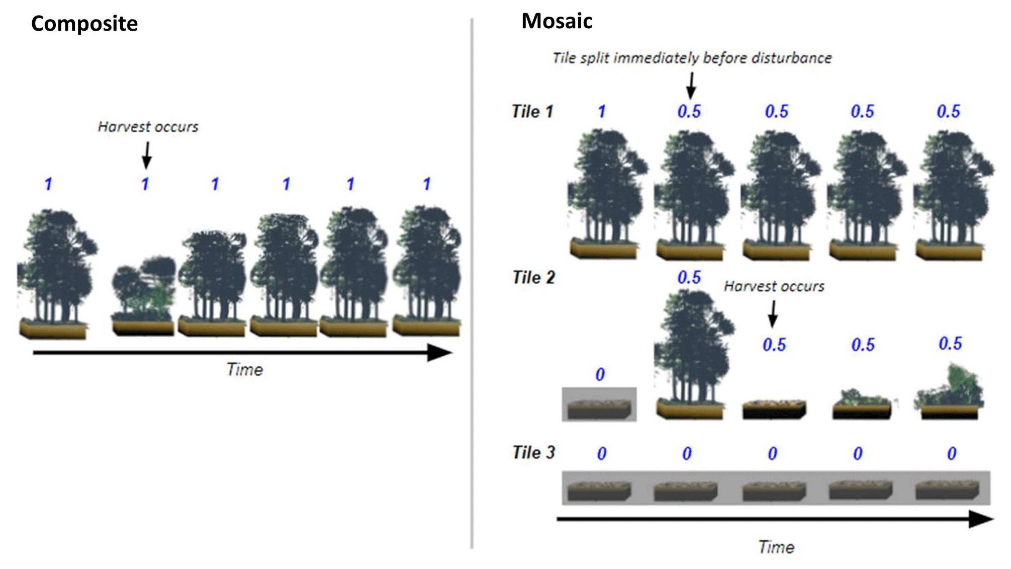
Figure 1 Illustrative diagram contrasting the composite (one tile) and mosaic (> 1 tile) representations of disturbance implemented herein. A hypothetical scenario where 50 % of a grid cell undergoes timber harvest is assumed here. The fraction of a grid cell that is occupied by a tile is denoted above each tile. Tiles that are not active have a gray background (e.g., tile 3 across all time steps).

2.3 Dynamic tile representation of externally forced fire and harvest

2.3.1 The composite versus mosaic representation in CLASSIC

CLASSIC can utilize either a composite (one tile) or mosaic (> 1 tile) representation of the land surface. The composite representation simulates average individual PFTs for each grid cell and uses their average structural attributes (i.e., leaf area index, height, and rooting depth) to simulate the energy balance and physical environment (i.e., soil temperature). The structural attributes of all of the average individual PFTs that exist within a grid cell are averaged in proportion to their fractional coverages, and the PFTs all experience a common land surface physical environment. For the composite representation, a disturbance event (i.e., wood harvest) takes an amount of C from the average individual PFT pools that is proportional to the areal fraction disturbed (i.e., a complete harvest of 50 % of the grid cell thereby removes 50 % of the vegetation biomass; Fig. 1).

The mosaic representation splits the grid cell into multiple tiles representing fractional areas of the grid cell. Each tile receives the same meteorological forcing but simulates its respective average individual of each PFT present, PFT structural attributes, and energy balance. The structural attributes of all the average individual PFTs that exist within each tile are averaged in proportion to their fractional coverages, and the PFTs all experience a land surface physical environment common to that tile. The tiles are aggregated to the scale of the final model grid by accounting for each tile's fractional coverage of the grid cell. CLASSIC's tiling capability has been used in the past to investigate the impacts of subgrid-scale heterogeneity in soil texture by breaking grid cells with heterogeneous soil textures into tiles (Melton et al., 2017), as well as vegetation cover (Melton and Arora, 2014; Li and Arora, 2012) and competition between plant functional types (Shrestha et al., 2016) by breaking grid cells with heterogeneous vegetation cover into tiles. These approaches result in regional differences in fluxes of up to 30 %. We adapt the mosaic representation to dynamically create disturbance history tiles and represent the subgrid-scale heterogeneity resulting from disturbance (i.e., we represent a complete harvest of an area corresponding to 50 % of the grid cell as a 100 % reduction of the vegetation biomass in a new subgrid tile that covers 50 % of the grid cell; Fig. 1). In our approach, the tiles serve to represent vegetation that is in different stages of recovery. Thus, the soil textures and vegetation fractional cover are the same for all tiles within a given grid cell.

2.3.2 Notation and background

We present generalized equations that illustrate the dynamic tiling calculations done by the model to split and join tiles. In these equations, scalars are lowercase letters (i.e., x = [1]), vectors are bold lowercase letters (i.e., x = $[x\mathrm{1},x\mathrm{2},\mathrm{\dots },xn]$), and matrices are bold uppercase letters (i.e., X = $\left(x_{\mathrm{1},\mathrm{1}}\mathrm{\cdots }{x}_{\mathrm{1},n}\mathrm{⋮}\mathrm{\ddots }\mathrm{⋮}{x}_{n,\mathrm{1}}\mathrm{\cdots }{x}_{n,n}\right)$. The model is set up to simulate state variables for a user-defined maximum number of tiles within a grid cell (i.e., the state variable x_all with a length equal to the user-determined maximum number of tiles). Tiles can be set as either active or inactive at each time step (Fig. 1). When the model identifies active tiles for merging or splitting (e.g., Sects. 2.3.4–2.3.6), they become candidate tiles. Depending upon the operation and the fraction of the grid cell involved, anywhere between one and the total number of tiles being actively simulated are candidate tiles for the merging or splitting operation. Because the maximum number of tiles is fixed, the model must manage the number of tiles being actively simulated. The model ensures that up to two inactive tiles are available to simulate disturbance each year (i.e., one for fire and one for harvest; see Sect. 2.3.4). During the merging or splitting operation, the model temporarily stores values from the candidate tiles before the operation (i.e., x_pre of length n, the total number of candidate tiles) and after the operation (i.e., x_post of length n, the total number candidate of tiles) and uses them to calculate the values for a new single output tile (i.e., x_new). All these values are temporarily stored and used in calculations up until the point where the dynamic tiling operation is complete, and the model's main data structures are updated.

2.3.3 Dynamic tiling splits and joins

Dynamic tiling allows the model to split grid cells into subgrid tiles during the model run or to join existing subgrid tiles. Dynamic tiling operations (splitting/joining) occur on 1 January at an annual time step alongside rigorous checks to ensure water, mass, and energy conservation. The area occupied by a given tile is a fraction of the grid cell land area between 0 and 1 (i.e., a_all with a length equal to the user-determined maximum number of tiles). The sum of a_all for all the active tiles within a grid cell must equal 1. When tiles are split, the fractional area occupied by the single new tile (a_new) must be less than the sum of the vector of fractional areas of the candidate tiles (a_pre of length n candidate tiles). The candidate tiles' fractional areas are a product of the dynamic tiling operations that occur in all previous time steps. When the first dynamic tiling operation in a run occurs, a_pre=[1], but a_pre is a much more complex vector in subsequent operations (e.g., ${\mathit{a}}_{\text{pre}}=[\mathrm{0.1},\mathrm{0.2},\mathrm{0.3}]$). The candidate tiles are later assigned a vector of new fractional areas adjusted to account for the new tile and the decrease in size of the candidate tiles (a_post, also of length n candidate tiles; Eq. 1).

$$\begin{array}{}\text{(1)}& {\displaystyle }\begin{array}{rl}& a_{\text{new}}<{\sum }_{i=\mathrm{1}}^n{a}_{\text{pre},i}\\ & a_{\text{post},n}=a_{\text{pre},n}-a_{\text{new}}{\displaystyle \frac{a_{\text{pre},n}}{{\sum }_{i=\mathrm{1}}^n{a}_{\text{pre},i}}}\end{array}\end{array}$$

When tiles are joined by the model, the fractional area of the new tile is the sum of the vector of the fractional areas of the candidate tiles. The candidate tiles are later assigned fractional areas of zero (Eq  2).

$$\begin{array}{}\text{(2)}& {\displaystyle }\begin{array}{rl}& a_{\text{new}}={\sum }_{i=\mathrm{1}}^n{a}_{\text{pre},i}\\ & {\mathit{a}}_{\text{post}}=\mathrm{0}\end{array}\end{array}$$

For a tile or group of tiles to be split or joined, they must pass rigorous checks that ensure they share the same abiotic characteristics and static fractional PFT cover. These characteristics (i.e., soil texture, soil permeable depth, and PFT fractional coverage) are copied directly to the new tile by the split or join. Mass-based variables (i.e., vegetation C pool mass, soil C pool mass, soil water, ponded water, and water held in the vegetation canopy) are split or joined using fractional-area-based weighted averages to ensure mass balance. The value of the mass-based variable in the new tile (M_new for l layers and o PFTs; kg m⁻²) is the average of the values for the candidate tiles (M_pre of length n candidate tiles for l layers and o PFTs; kg m⁻²) weighted by the fractional areas of the candidate tiles (Eq. 3).

$$\begin{array}{}\text{(3)}& m_{\text{new},lo}={\displaystyle \frac{{\sum }_{i=\mathrm{1}}^n{m}_{\text{pre},ilo}{a}_{\text{pre,i}}}{{\sum }_{i=\mathrm{1}}^n{a}_{\text{pre},i}}}\end{array}$$

Temperature-based variables (i.e., the temperatures of the vegetation canopy, ponded water, snowpack, and soil) are split or joined using a fractional area-based weighted average that blends the different temperature materials from the candidate tiles. The value of a given temperature for the new tile (t_new for l layers; K) is a function of the temperatures in the candidate tiles (T_pre of length n candidate tiles for l layers; K) weighted by the fractional areas of the candidate tiles before the split, the masses of the pools which track that temperature (M_pre of length n candidate tiles for l layers and m pools; kg m⁻²), and the specific heat capacities which characterize those mass pools (c for m pools; $\mathrm{J}{\mathrm{kg}}^{-\mathrm{1}}{\mathrm{K}}^{-\mathrm{1}}$; Eq. 4).

$$\begin{array}{}\text{(4)}& t_{\text{new},l}={\displaystyle \frac{{\sum }_{i=\mathrm{1}}^n\left(t_{\text{pre},il}{a}_{\text{pre},i}{\sum }_{j=\mathrm{1}}^m\left(m_{\text{pre},ilj}{c}_j\right)\right)}{{\sum }_{i=\mathrm{1}}^n\left(a_{\text{pre},i}{\sum }_{j=\mathrm{1}}^m\left(m_{\text{pre},ilj}{c}_j\right)\right)}}\end{array}$$

2.3.4 Dynamic tiling management

The maximum number of dynamic tiles in a given simulation is limited by a parameter set at the start of the model run. If this upper limit is reached, tiles are joined based on a similarity criterion. By default, the model selects the two tiles with the most similar vegetation heights and joins them. The model uses the vector of tile average vegetation heights ( of length n for the total number of tiles; m) and calculates the absolute differences between all possible combinations of the elements therein (i.e., using the nested iterators n1 and n2). The resulting absolute difference matrix of tile average vegetation heights (, a n1 total number of tiles by n2 total number of tiles matrix; m) is used to judge the similarity between tiles. The tile average vegetation height is a function of each PFT height (H of length n, the total number of tiles, for o PFTs; m) and the PFT fractional coverage within the tile (F of length n, the total number of tiles for o PFTs; Eq. 5; Fig. S1 in the Supplement). In the default case, the two tiles with the minimum are joined when the maximum number of dynamic tiles is reached.

$$\begin{array}{}\text{(5)}& {\displaystyle }\begin{array}{rl}& \mathrm{\Delta }{}_{n\mathrm{1},n\mathrm{2}}=\left|{}_{n\mathrm{1}}-{}_{n\mathrm{2}}\right|\\ & {}_n={\displaystyle \frac{{\sum }_{o=\mathrm{1}}^{\mathit{\#}\text{ of PFTs}}{h}_{n,o}{f}_{n,o}}{{\sum }_{o=\mathrm{1}}^{\mathit{\#}\text{ of PFTs}}{f}_{n,o}}}\end{array}\end{array}$$

An optional relative height threshold (rht; unitless) allows for tiles to be pre-emptively joined at a yearly time step before the maximum number of dynamic tiles is reached. rht can be conceptually thought of as breaking the tiles into equally spaced bins organized by vegetation height. It is used to calculate a threshold value from the maximum tile average vegetation height (; m). The threshold logically determines which pairs of tiles are pre-emptively joined at a yearly time step based on the absolute differences in their tile average vegetation heights (; m; Eq. 6; Fig. S1).

$$\begin{array}{}\text{(6)}& \textcolor{red}{}<\text{rht}\cdot max\left(\textcolor{red}{}\right)\end{array}$$

When the rht parameter is used, the optional tile preservation parameter (tpp; number of tiles) prevents tiles with the shortest average vegetation height from being merged. tpp is an integer which determines the number of tiles that the model will retain, starting from the tile with the shortest average vegetation height. This means the tiling scheme will carry out pre-emptive joins based upon rht while preserving young recently disturbed tiles and explicitly representing early successional differences in fluxes (Bellassen et al., 2010; Zaehle et al., 2006; Nabel et al., 2020). When dynamic tiling is active, the time since disturbance is tracked for all tiles. Time since disturbance increases at the CTEM time step (i.e., daily). Any disturbance event applied to a particular tile resets its time since disturbance to zero.

2.3.5 Externally forced fire

Externally forced fire builds upon the pre-existing fire module within CLASSIC (Melton and Arora, 2016; Arora and Melton, 2018). The annual fractional burned area in a grid cell is read from a file. The model assumes that fire impacts all non-crop PFTs.

If dynamic tiling is not active, biomass from the average individual and the litter pool burns proportional to the requested fractional burned area. If dynamic tiling is active, a new tile with a fractional area equal to the fractional burned area is split from the active tiles within the grid cell and subsequently burned. Depending upon the requested fractional burned area and the conditions in the grid cell, the model uses anywhere between one tile and the total number of tiles being actively simulated as candidate tiles for this splitting operation.

To determine the candidate tiles for this splitting operation, the model ranks the tiles based on their probability of fire (p of length n) conditional on the total aboveground biomasses available for burning (b of length n; kg C m⁻²). p is a linear function of the lower biomass threshold (0.4 kg C m⁻²) under which fire cannot sustain itself and the upper biomass threshold over which fire has a probability of 1 (1.2 kg C m⁻²; Eq. 7) (Moorcroft et al., 2001; Kucharik et al., 2000; Melton and Arora, 2016).

$$\begin{array}{}\text{(7)}& p_n=max\left[\mathrm{0},min\left(\mathrm{1},{\displaystyle \frac{b_n-\mathrm{0.4}}{\mathrm{1.2}-\mathrm{0.4}}}\right)\right]\end{array}$$

Table 1 The PFT-specific fire emission fractions (υ) used to calculate C emissions to the atmosphere due to fire for each live vegetation component (i.e., both structural and non-structural leaves, stems, and roots) and the litter pool as well as the PFT-specific mortality fractions (Θ) used to calculate the quantity of C from each live vegetation component transferred to the litter pool. Crop PFTs are not impacted by fire and are therefore not assigned fractions (Melton and Arora, 2016).

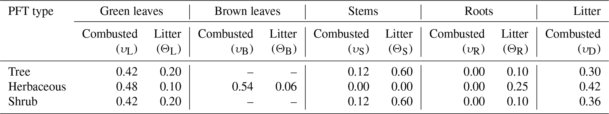
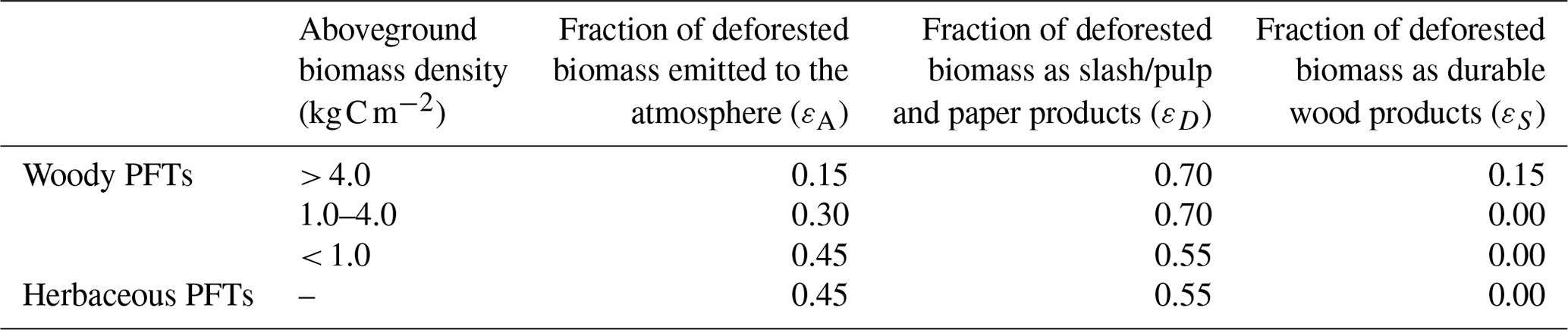
Table 2 The fractions of harvest-affected biomass transferred to different wood product pools for herbaceous PFTs and woody PFTs (ε). The fractions for woody PFTs differ depending on the aboveground biomass density (Arora and Boer, 2010).

The model initially selects tiles with a p of 1 as candidate tiles to be split to yield the tile to be burned. However, if these selected tiles do not contain enough fractional area to simulate the fractional burned area requested, the model selects tiles with a p of less than 1 from largest to smallest (Fig. S1). Externally forced fire uses a single probability (p) to rank tiles, whereas CLASSIC's standard fire module uses three probabilities to calculate the burned area: the probability of fire conditional on the total aboveground biomasses available for burning, the combustibility of the fuel based on its moisture content, and the presence of an ignition source (Arora and Boer, 2005; Arora and Melton, 2018). We make this simplification here because the fractional burned area comes from a file and all the tiles within a grid cell experience the same driving meteorology, limiting differences in moisture content and ignition (Melton et al., 2017; Melton and Arora, 2014). With dynamic tiling either active or inactive, we calculate the C emissions to the atmosphere using pre-defined PFT-specific fire emission fractions for each live vegetation component (i.e., both structural and non-structural leaves, stems, and roots) as well as the litter pool (υ; Table 1). We calculate the quantity of live vegetation C transferred to the litter pool as a result of fire-related mortality using pre-defined PFT-specific mortality fractions (Θ; Table 1). Externally forced fire does not impact crop PFTs, and thus their biomass never combusts nor experiences fire-related mortality.

2.3.6 Externally forced harvest

Harvest simulates the removal of biomass from the landscape because of logging activities and builds upon the pre-existing land use change module within CLASSIC (Arora and Boer, 2010). The annual fractional harvested area on a per-grid-cell basis is read from a file. The model assumes that all harvest events are clearcuts that impact some fraction of the simulated grid cell.

If dynamic tiling is not active, the average individual is harvested proportional to the requested fractional area. If dynamic tiling is active, a new tile with a fractional area equal to the requested fractional area is split from the oldest undisturbed active tile, and the entire new tile is harvested. If the harvested area requested exceeds the fractional area of the oldest undisturbed active tile, the model selects additional active tiles as candidate tiles from oldest to youngest until there is sufficient fractional area.

In either case, the harvested aboveground biomass (i.e., both non-structural and structural stem and leaf C) is split into three streams using fractions developed by Arora and Boer (2010). These streams contribute C to the atmosphere, the slash/pulp and paper product pool, and the durable wood product pool. The fractions of harvested aboveground biomass allocated to each stream (ε; Table 2) depend upon whether the PFT is woody or herbaceous and, in the case of woody PFTs, the aboveground biomass density. Unlike the procedure described by Arora and Boer (2010) where root biomass is transferred to the slash/pulp and paper product pool, we transfer harvested root biomass to the applicable PFT and soil-depth-specific litter pools.

2.4 Model forcing

2.4.1 Meteorological drivers and land cover

CLASSIC requires seven meteorological forcing variables: incoming shortwave radiation, incoming longwave radiation, air temperature, precipitation rate, air pressure, specific humidity, and wind speed. We use the interpolated and disaggregated meteorological forcing described in detail by Meyer et al. (2021) and Curasi et al. (2023b) (GSWP3–W5E5–ERA5) in our simulations. The 1901–1978 portion of the forcing comes from the Inter-Sectoral Impact Model Intercomparison Project GSWP3–W5E5 and the 1979–2018 portion comes from the ERA5 time series bias-corrected to match the means of the overlapping period in the GSWP3–W5E5 (Kim, 2017; Lange, 2019, 2020a, b; ECMWF, 2019). The atmospheric CO₂ concentrations (1700–2017) were obtained from the global carbon project (“Trends in atmospheric carbon dioxide”, National Oceanic & Atmospheric Administration, Earth System Research Laboratory (NOAA/ESRL), 2022; Friedlingstein et al., 2022).

We set the fractional coverage of PFTs using the remotely sensed 14 PFT-hybrid land cover product generated by Wang et al. (2023) and expanded upon and evaluated by Curasi et al. (2023b). This land cover corresponds to the year 2010. This land cover product combines information from the North American Land Change Monitoring System land cover (Latifovic et al., 2017), the National Terrestrial Ecosystem Monitoring System (NTEMS) (Hermosilla et al., 2018, 2016), satellite-derived maps of the National Forest Inventory attributes (Beaudoin et al., 2018), and British Columbia's biogeoclimatic ecosystem classification map (MacKenzie and Meidinger, 2018; Salkfield et al., 2016). Using a land cover that does not vary in time (i.e., static land cover as opposed to dynamic or prescribed land cover changes) allows us to focus on the influences of fire, harvest, and dynamic tiling on the model outputs.

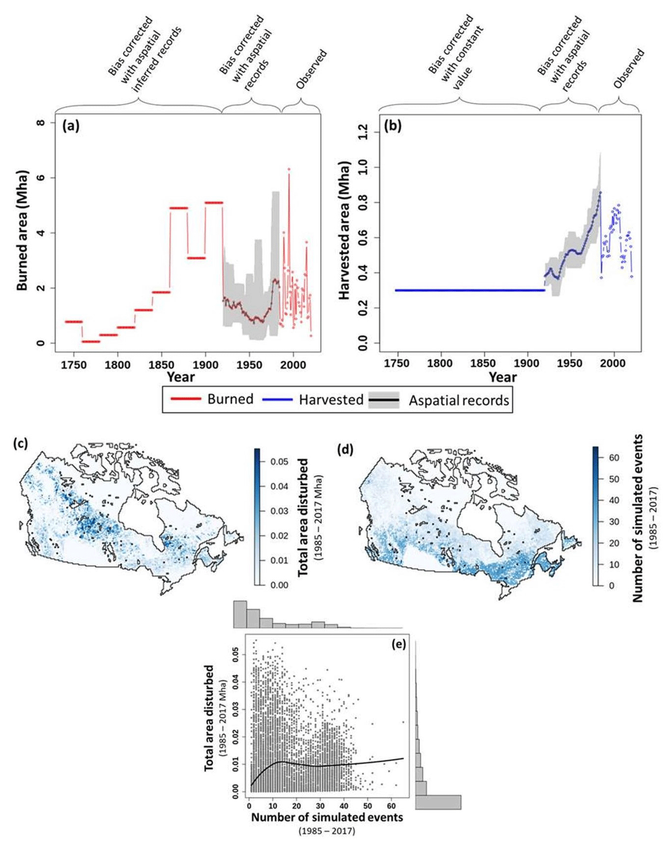
Figure 2 Plots of the disturbance drivers over time. Annual total (a) burned and (b) harvested areas from 1740–2020. “Observed” indicates the period that uses the Landsat fire and harvest observations (Hermosilla et al., 2016, 2015a, b). “Bias-corrected with aspatial records” indicates the period where the disturbance was inferred from the 2019 stand age (Maltman et al., 2023) and bias-corrected using the aspatial harvested and burned areas (Skakun et al., 2021; World Resources Institute, 2000; Van Wagner, 1988). “Bias-corrected with aspatial inferred records” and “Bias-corrected with constant value” indicate the period where the inferred disturbance was bias-corrected based on Kurz et al. (1995) and Chen et al. (2000), respectively. The aspatial records line is the 9-year running mean, min, and max of the aspatial total harvested and burned area data sets. (c) Per-grid-cell total area disturbed (1985–2017) and (d) the total number of simulated events (1985–2017). (e) Per-grid-cell total area disturbed, excluding undisturbed cells, plotted against the total number of simulated events. The black line is a LOESS curve. Note that a simulated event combines all the individual fire or harvest events that occur in a grid cell in a single year, with a maximum of two simulated events per year (one fire and one harvest) occurring in each grid cell.

2.4.2 Fire and harvest forcing

We develop fire and harvest drivers that detail the per-grid-cell annual fractional area harvested or burned between 1740 and 2017 (Fig. 2a and b). For the satellite era (1985–2017), we use remotely sensed 30 m spatial resolution records of harvest and fire events. These data were derived from Landsat by using breakpoint detection to identify changes and trends (Hermosilla et al., 2016, 2015a) followed by a random forest classification of change types (Hermosilla et al., 2015b). We mask the remotely sensed harvest records to include only private, long-term tenure, and short-term tenure forests, as indicated by Stinson et al. (2019).

Before the availability of remotely sensed records used herein (pre-1984), to our knowledge, there are no spatially explicit pan-Canadian integrated harvest and fire data sets available. Therefore, to represent the impact of historical disturbance on the model state, we employ established methods for inferring disturbance events from stand age (Nabel et al., 2020; Kurz et al., 2009; Chen et al., 2000, 2003). We also focus our analysis of the CLASSIC simulations on the satellite era (1985–2017) due to uncertainties in inferred historical disturbance and the model state before the satellite era. Maltman et al. (2023) derived a 30 m resolution stand-age map for 2019 from Landsat and MODIS data utilizing three methods. The methods included disturbance detection for stands between 0 and 34 years of age, the detection of spectral signals indicative of recovery for stands between 34 and 54 years of age, and inverting allometric equations for stands between 54 and 150 years of age. We infer the year in which the last disturbance occurred from the stand age. For example, a 40-year-old forest in 2019 is assumed to have been last disturbed in 1979. We use regional averages of the per-pixel ratio of burned to total disturbed area from the first decades of the satellite era (1985–1995) to fraction total inferred disturbance into fire and harvest.

However, pre-1984 disturbance that has been inferred from stand age does not align with available aspatial records of total harvested and burned area within Canada. Therefore, we utilize the aspatial records to bias-correct the 1740–1984 disturbance that has been inferred from stand age to ensure that the total values match the available historical records. From 1740–1920, we utilized aspatial records of total disturbed area derived from 1920 stand age with harvest held constant (0.3 Mha yr⁻¹) (Chen et al., 2000; Kurz et al., 1995). From 1920–1984, we utilized aspatial records of the total harvested and burned area within Canada from Skakun et al. (2021) and World Resources Institute (2000). We utilize bias correction that retains the spatial patterns of pre-1984 disturbance inferred from stand age while correcting positive and negative biases to match the aspatial records. This necessitated two distinct bias correction methods. For years with positive biases, the positive bias indicates that sufficient disturbance is inferred from stand age. In these cases, a uniform bias correction factor can be used to scale down disturbance. Years with negative biases, however, do not contain sufficient disturbance as inferred from stand age. Here, residual disturbed area from nearby years needs to be added to the year under consideration to match the aspatial records' level of disturbance while preserving the spatial patterns derived from stand age. Because the uncertainty of stand age estimates increases further into the past, the negative bias correction is carried out starting in 1984 and looping backward annually until 1740 (Maltman et al., 2023).

First, for years in which burned or harvested area inferred from stand age (D_inferred for i years, l grid cells; m²) exceeded the aspatial records (d_aspatial for i years; m²), we correct the positive biases. We calculate an aspatial bias correction factor (f for i years; unitless; Eq. 8).

$$\begin{array}{}\text{(8)}& f_i={\displaystyle \frac{\left(\left({\sum }_{l=\mathrm{1}}^{\mathit{\#}\text{ of grid cells}}{\mathit{d}}_{\text{inferred},i,l}\right)-{\mathit{d}}_{\text{aspatial},i}\right)}{\left({\sum }_{l=\mathrm{1}}^{\mathit{\#}\text{ of grid cells}}{\mathit{d}}_{\text{inferred},i,l}\right)}}\end{array}$$

Because the pre-1985 records are aspatial, the bias correction factor is temporally explicit but uniformly applied across space. When we apply the bias correction factor to the inferred disturbance time series, the result is a new time series with all the positive biases corrected (D_downsc for i years, l grid cells; m²; Eq. 9).

$$\begin{array}{}\text{(9)}& d_{\text{downsc},il}=d_{\text{inferred},il}-d_{\text{inferred},il}{f}_i\end{array}$$

When we apply the bias correction factor, we retain the spatially and temporally explicit residuals (D_residual for i years, l grid cells; m²; Eq. 10).

$$\begin{array}{}\text{(10)}& d_{\text{residual},il}=d_{\text{inferred},il}-d_{\text{downsc},il}\end{array}$$

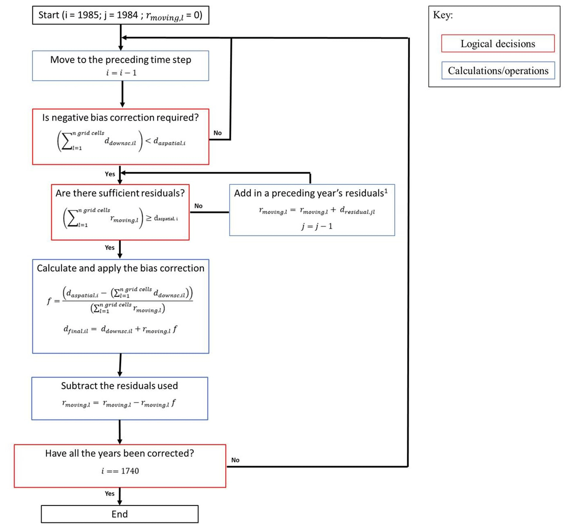
Figure 3 A schematic diagram of the negative bias correction algorithm with applicable equations and logical tests. ¹ Not shown: when the spatially explicit residuals are exhausted, they are replenished using the entire remotely sensed and stand-age-inferred disturbance record.

Second, for years in which burned or harvested area inferred from stand age falls below that indicated in the aspatial records, we correct the negative biases by adding in the residuals from nearby years (Fig. 3). We loop backward in time from 1984 to 1740 and accumulate residuals (r_moving for l grid cells; m²) extending as far back in time as needed to exceed the aspatial record for the year under consideration (d_aspatial,i). We calculate an aspatial bias correction factor (f; unitless) and use it to apply a fraction of r_moving to the inferred disturbance time series and subtract the residuals used from r_moving. When the spatially explicit residuals are exhausted (∼ 1920 for fire only), they are replenished using the entire gridded remotely sensed and stand-age-inferred disturbance record. This procedure continues until all the negative biases have been corrected between 1984 and 1740, yielding the final spatially explicit time series (D_final for i years, l grid cells; m²).

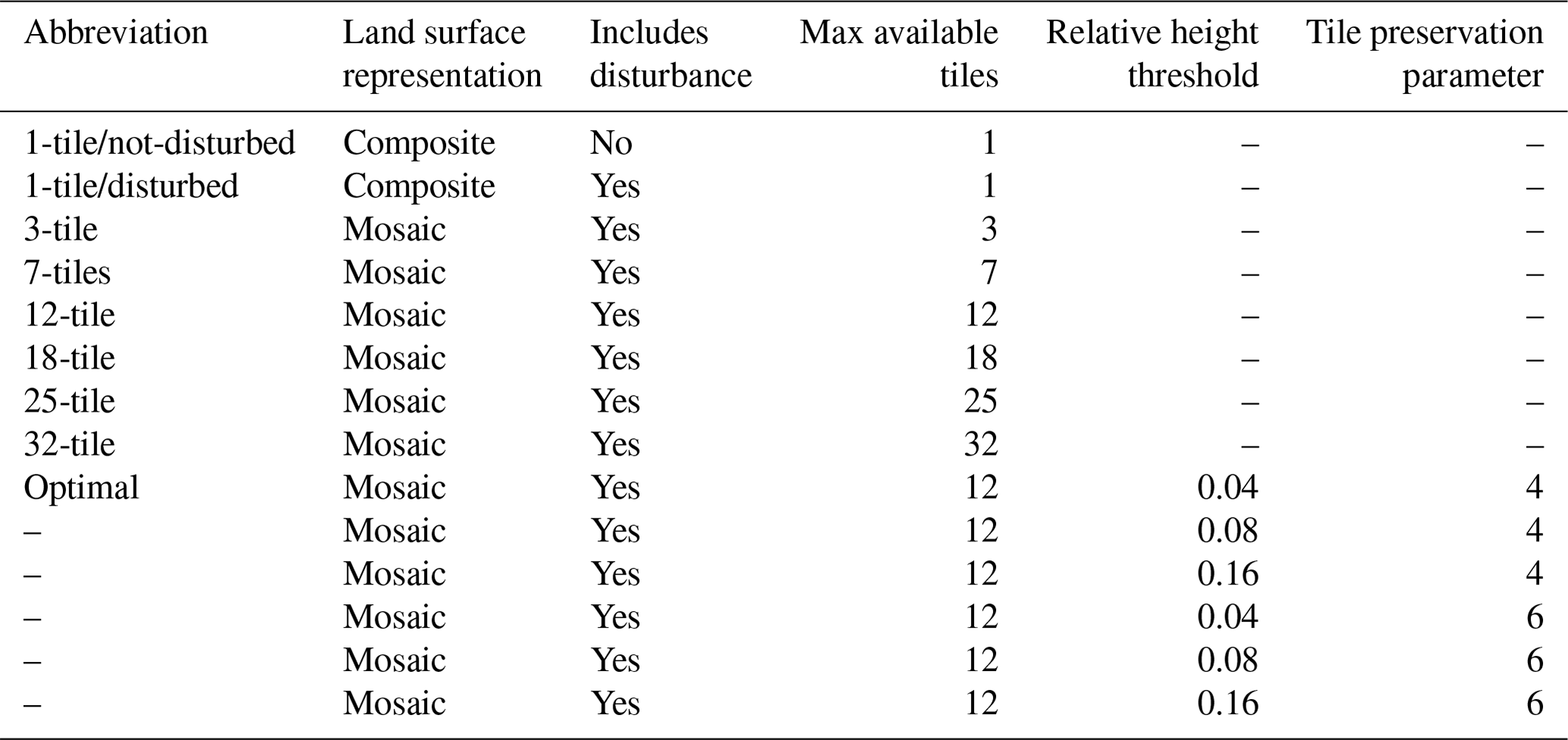
Table 3 An overview of the simulations conducted in this study.

2.5 Simulation protocol

We carry out a total of 14 simulations using a common simulation protocol to investigate the impacts of different maximum numbers of available tiles, rht, and tpp (Table 3). rht (0.04–0.16, unitless) can be conceptually thought of as breaking the range of tile average vegetation heights into between 24 and six equally spaced bins, depending upon its value (e.g., (1 bin m m⁻¹$/$6 bins) = 0.16 m m⁻¹). tpp (4–6 tiles) can be conceptually thought of as the maximum number of discrete disturbance events that the model can simulate in a grid cell over 2–3 years (e.g., (1 harvest tile yr⁻¹ + 1 fire tile yr⁻¹) × 3 years × 6 tiles).

We spin up the model to equilibrium conditions corresponding to the year 1700 and then do a transient run over the period 1700 to 2017. For the spin up, we loop the earliest 25 years of climate data available (1901–1925) and hold atmospheric CO₂ concentrations constant at the pre-industrial (1700) level. The 1700–1900 portion of the transient run uses the same loop of 1901–1925 climate but transient atmospheric CO₂ concentrations. The 1900–2017 portion of the transient run uses transient atmospheric CO₂ concentrations and evolving GSWP3–W5E5–ERA5 climate. During the full transient simulation from 1740–2017, the fire and harvest are applied (see Sect. 2.4). The 14 transient simulations utilize their individual, unique land-surface representation (i.e., composite or mosaic), maximum number of available tiles, rht, and tpp for the entire 1700–2017 run (Table 3). The CLASSIC nitrogen cycling module is not active in these simulations (Asaadi and Arora, 2021; Arora and Boer, 2010).

2.6 Model evaluation

We carry out model-on-model comparisons for a selection of variables and model configurations for the satellite era portions of our simulations (1985–2017) to select the model setup that optimally balances a detailed process representation and model run time (Table 3). This model-on-model approach has the benefit of canceling out any pre-existing biases in the model and focusing our results on the impacts of subgrid-scale heterogeneity, and discretization error (similar to Torres-Rojas et al., 2022; Moorcroft et al., 2001). We also use these evaluations to demonstrate the relative impact of representing subgrid-scale heterogeneity within our modeling framework. We evaluate a suite of C cycling and surface-energy-balance-related variables, including the land carbon pool (cLand), vegetation C (cVeg), soil C (cSoil), gross primary productivity (GPP), autotrophic respiration (Ra), heterotrophic respiration (Rh), ecosystem respiration (ER), leaf area index (LAI), sensible heat flux (HFSS), latent heat flux (HFLS), albedo (ALBS), fire emissions (fFire), total deforested C (fDeforestTotal), and cumulative deforested C (the running sum of fDeforestTotal starting in 1985; fDeforestCumulative).

To select the optimal maximum number of tiles available for the simulation as well as the rht and tpp, we calculate the mean squared deviation (msd for the j model runs detailed in Table 3 over the 1985–2017 period) between the model runs under evaluation and the reference 32-tile run. The 32-tile run is the reference point, as it is the simulation with the least compromise between run time and simulation detail and is assumed to best represent the impacts of disturbance in CLASSIC. MSD represents the mean of the squared differences between the annual summary (i.e., means for fluxes and sums for pools) of each variable for the 32-tile run (${\widehat{\mathit{x}}}_{\text{32tile}}$ containing i years) and that for the simulations under evaluation ($\widehat{\mathbf{X}}$ containing i years for j model runs; Eq. 11).

$$\begin{array}{}\text{(11)}& {\text{msd}}_j={\displaystyle \frac{\mathrm{1}}{\mathrm{33}}}{\sum }_{i=\mathrm{1985}}^{\mathrm{2017}}{\left({\widehat{x}}_{j,i}-{\widehat{x}}_{\text{32tile},i}\right)}^{\mathrm{2}}\end{array}$$

We also use a normalized response metric ($\mathbf{\Delta }{\stackrel{\mathrm{‾}}{\mathbf{X}}}_{\text{norm}}$ for j model runs, k variables; Eq. 12) to evaluate the relative impacts of disturbance and subgrid-scale heterogeneity on the simulations. The normalized response metric is a unitless summary statistic. Its strength is that a wide range of variables with different units can be visualized on the same axis to make relative comparisons of their simulated responses to disturbance and tiling. For a given variable, the metric normalizes each variable's output (X for i years, j model runs, k variables, l grid cells) using the minimum and maximum across all the outputs (X_norm for i years, j model runs, k variables, l grid cells; Eq. 12). Each normalized variable is averaged across the model domain and run years (${\stackrel{\mathrm{‾}}{\mathbf{X}}}_{\text{norm}}$ for j model runs, k variables; 1985–2017) considering each model grid cell's area (a_{grid  cell}; m²). Finally, the absolute value of the difference between ${\stackrel{\mathrm{‾}}{\mathbf{X}}}_{\text{norm}}$ for the desired runs (the 1-tile/not-disturbed and 32-tile runs) and the 1-tile/disturbed run is calculated (Eq. 12).

$$\begin{array}{}\text{(12)}& {\displaystyle }{x}_{\text{norm},i,j,k,l}={\displaystyle \frac{(x_{i,j,k,l}-min(X_k\left)\right)}{(max(X_k)-min(X_k\left)\right)}}\text{(13)}& {\displaystyle }\begin{array}{rl}& {\stackrel{\mathrm{‾}}{x}}_{\text{norm},j,k}=\\ & {\displaystyle \frac{{\sum }_{i=\mathrm{1985}}^{\mathrm{2017}}\left({\sum }_{l=\mathrm{1}}^{\mathit{\#}\text{ of grid cells}}{x}_{\text{norm},i,j,k,l}{a}_{\text{grid cell},l}\right)}{\mathrm{33}\left({\sum }_{l=\mathrm{1}}^{\mathit{\#}\text{ of grid cells}}{a}_{\text{grid cell},l}\right)}}\end{array}\text{(14)}& {\displaystyle }\mathrm{\Delta }{\stackrel{\mathrm{‾}}{x}}_{\text{norm},j,k}=\left|{\stackrel{\mathrm{‾}}{x}}_{\text{norm},j,k}-{\stackrel{\mathrm{‾}}{x}}_{\text{norm},\text{1-tile}/\text{disturbed},k}\right|\end{array}$$

All plots are created using R or the External Dynamic and Interactive Framework Integrating CLASSIC Experiments (EDIFICE) Python suite (Hijmans et al., 2015; R Core Team, 2013).

3 Results and discussion

3.1 Disturbance events within Canada

For the period represented by satellite data in this study, the highest total disturbed areas are in central boreal regions of the country and are attributable to wildfire events (Fig. 2c). In contrast, harvest is concentrated on the west coast and in eastern boreal and maritime regions of the country. The annual total disturbed area differs widely between years during the satellite era (Fig. 2a and b). In aggregate, harvest occurs in ∼ 2 % of the land area modeled, and fire occurs in ∼ 6 % from 1985 to 2017. The total number of simulated disturbance events is moderate, with 89 % of the grid cells incorporating 32 or fewer simulated disturbance events during the satellite era and 61 % incorporating 11 or fewer (Fig. 2d and e). Our aspatial tiling scheme operates on an annual time step, and therefore the maximum number of possible events in the 1985–2017 drivers is 66 (i.e., a harvest and fire each year for 33 years; Fig. 2e). Generally, beyond 11 simulated disturbance events, there is a limited correlation between the number of simulated disturbance events and the total area disturbed (Fig. 2e).

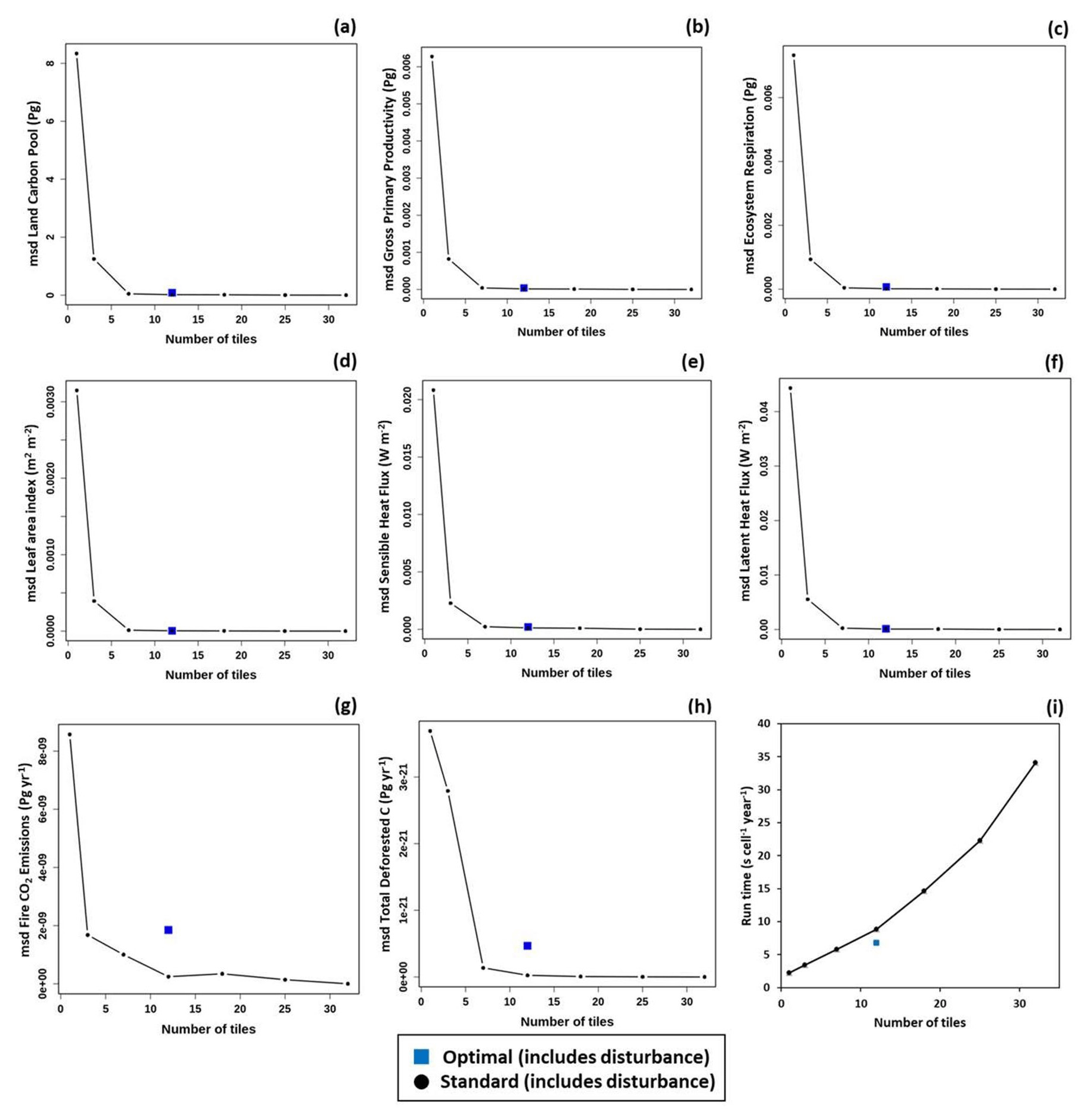
Figure 4 Plots of the mean squared deviation (msd; 1985–2017; Eq. 11) for (a) the land carbon pool (cLand), (b) gross primary productivity (GPP), (c) ecosystem respiration (ER), (d) leaf area index (LAI), (e) sensible heat flux (HFSS), (f) latent heat flux (HFSS), (g) fire emissions (fFire), and (h) total deforested carbon (fDeforestTotal) for model runs including disturbance with varying numbers of tiles (1–32) compared against the run including disturbance with the largest number of tiles (32). (i) The run time for each configuration. Values are also shown for the optimal model run including disturbance with 12 tiles (tile preservation parameter, tpp = 4; relative height threshold, rht = 0.16).

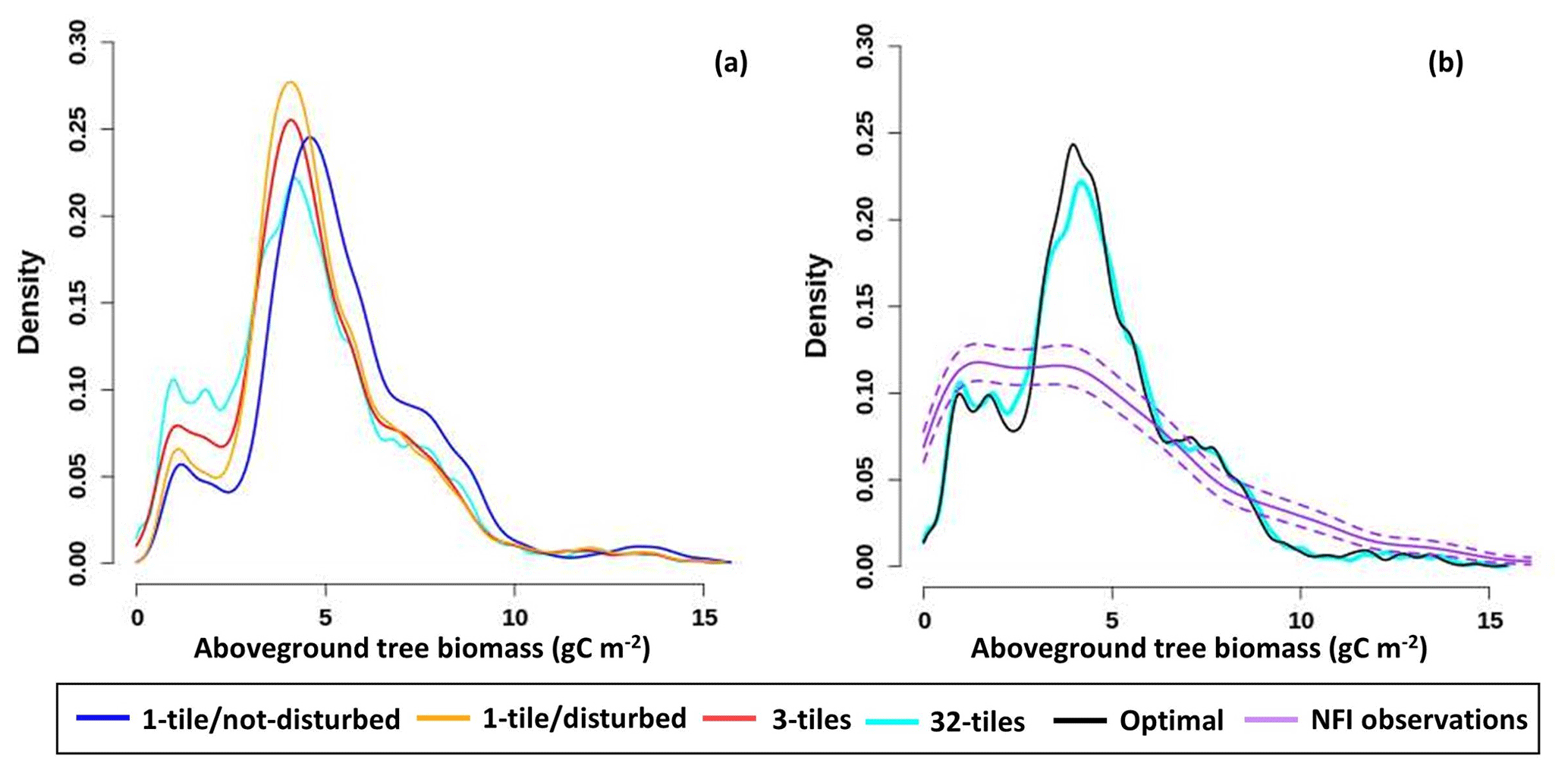
Figure 5 Weighted histogram of aboveground tree biomass for forested areas of Canada (a) at the end of a selection of model runs, including the 1-tile/not-disturbed run, 1-tile/disturbed, 3-tiles, and 32-tiles, as well as for (b) 32-tiles, optimal (12 tiles, four preserved tiles, and a threshold of 0.16), and observations from the National Forest Inventory (NFI) (Gillis et al., 2005). All runs using > 1 tile include disturbance. The bootstrapped 95 % CI for the NFI observations is also shown. The contributions of all forested subgrid areas weighted by their fractional area within the modeled region are considered. An area is classified as forested if it contains at least 50 % tree cover.

3.2 Model parameterization

The change in the MSD (Fig. 4a–h) as the maximum number of available tiles for the run increases from 1 to 32 exhibits a roughly exponential decline for the surface energy balance (HFSS, HFLS) and C-cycle-related variables (cLand, GPP, ER, LAI). The MSD is near zero at 7–12 tiles. The 32-tile simulation captures all the discrete disturbance events from 1985–2017 across most of the model domain (Fig. 2). However, a simulation that resolves all the disturbance events between 1740 and 2017 as tiles would require far more than 32 tiles in many forested areas and would be computationally intractable. However, we infer from the exponential (e.g., rather than linear) decreasing rate of change in Fig. 4a–f that our reference 32-tile simulation has minimal discretization error and converges on the results of that computationally intractable simulation (Torres-Rojas et al., 2022; Nabel et al., 2020; Nocedal and Wright 2006). The difference in MSD between the 32-tile simulation and that computational intractable simulation would likely be vanishingly small, similar to the difference between the 25-tile and 32-tile simulations (Nabel et al., 2020; Fisher et al., 2018; Ellner and Guckenheimer, 2011; Gelman and Hill, 2006). These roughly exponential declines in MSD reflect the model's ability to discretize patches of vegetation in different stages of recovery using greater numbers of tiles. This is reflected in how the statistical distributions of aboveground tree biomass in forested grid cells change as more tiles are utilized in the simulation (Fig. 5a).

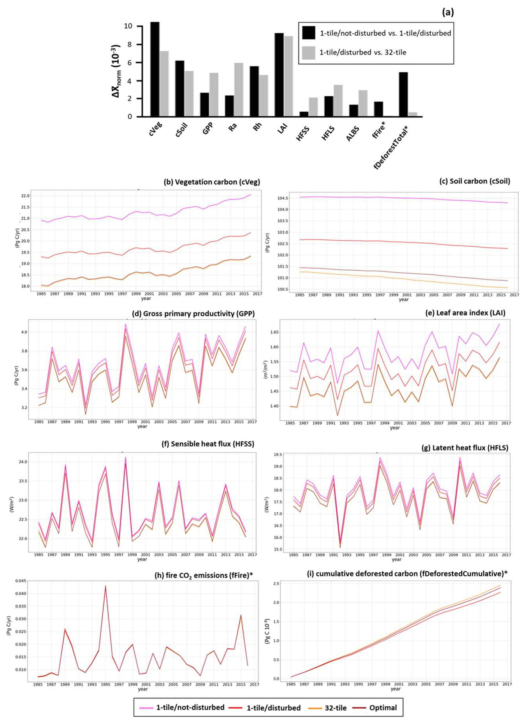
Figure 6 (a) Plot of the normalized response metric ($\mathrm{\Delta }{\stackrel{\mathrm{‾}}{\mathbf{X}}}_{\text{norm}}$; Eq. 12) for 1-tile/not-disturbed versus 1-tile/disturbed and for 1-tile/disturbed versus 32-tile for vegetation carbon (cVeg), soil carbon (cSoil), gross primary productivity (GPP), autotrophic respiration (Ra), heterotrophic respiration (Rh), leaf area index (LAI), sensible heat flux (HFSS), latent heat flux (HFLS), albedo (ALBS), fire emissions (fFire), and total deforested carbon (fDeforestTotal). Time series plots of (b) cVeg, (c) cSoil, (d) GPP, (e) LAI (f) HFSS, (g) HFLS, (h) fFire, and (i) cumulative deforested carbon (fDeforestCumulative; the running sum of fDeforestTotal starting in 1985) for 1-tile/not-disturbed, 1-tile/disturbed, 32-tile, and optimal (tpp = 4; rht = 0.16; purple). All runs using > 1 tile include disturbance. In panel (a), a normalized response of zero indicates that there are no differences between the runs. ^∗ These are disturbance-related fluxes that are omitted in the 1-tile/not-disturbed model run.

Disturbance-related variables, including fFire as well as fDeforestedTotal, exhibit a less sharp decline when going from one to seven tiles and approach zero at 12 tiles (Fig. 4g and h). This reflects the influence of selecting and splitting tiles in different phases of recovery on these processes and the extent to which recovering tiles with lower aboveground tree biomass are represented in the simulation (Fig. 5a). As a result, there is a discontinuity between representing these processes using average individuals, a small number of highly heterogeneous tiles, and many tiles (Figs. 4g and h and 5a). This pattern is also likely influenced by the relatively low magnitude of the differences between the simulations compared to the fluxes themselves (Fig. 6a, h, and i).

The run time for the satellite-era simulation (1985–2017) with one tile is ∼ 318 CPU hours (i.e., the sum of time utilized by all cores across multiple machines; Xeon Platinum 8380). Compared to the 1-tile run, the 32-tile, 12-tile, and optimal runs consume 14 times, 3 times, and 2 times as many CPU hours, respectively. The run time of the simulations increases linearly between one and 12 tiles (Fig. 4i) but increases more rapidly from 18 to 32 tiles due to the increasingly large multidimensional per-tile structures in memory. The intercept (i.e., the overhead for pre-processing meteorological files and initializing message passing interface sessions to run the model with a single tile) is around 3 times the slope (i.e., the time required to run each additional tile) for simulations with less than 12 tiles. This suggests that the splitting operations involved in simulating additional tiles are computationally efficient and do not dramatically increase the run time (Nabel et al., 2020).

As with all modeling exercises, we must balance model accuracy, complexity, and computational efficiency. We, therefore, use simulations with 12 tiles to set the rht (i.e., the relative height threshold for pre-emptively joining tiles) and tpp (i.e., the number of preserved recently disturbed tiles) parameter values. Simulations using 12 tiles and different rht and tpp parameters are very similar in terms of run time, and the surface energy balance and C-cycle-related variables exhibit no consistent patterns (Fig. S2a–f and i). There is a gradual increase in MSD for fFire and fDeforestedTotal as rht and tpp increase (Fig. S2g–h). However, these differences are again of relatively low magnitude compared to the fluxes themselves (Fig. 6a, h, and i). Therefore, we chose an rht of 0.16 and a tpp of 4 to maximize computation efficiency. The optimal parameterization has MSD values similar to those of a run with 12 tiles but with a lower run time (∼ 23 % less; Fig. 4i). The optimal model nearly approximates the heterogeneous tile structure of the more complex 32-tile simulation and represents forested areas with low aboveground tree biomass like the 32-tile simulation, in line with observations of aboveground tree biomass from the NFI (Fig. 5b). However, it may over-smooth the transition between low- and high-biomass areas (i.e., the ∼ 2–3 g C m⁻² range in Fig. 5b), thereby impacting the size classes of the tiles selected for splitting during the disturbance simulation (Fig. 4g and h). Nonetheless, the optimal simulation effectively balances computational efficiency and discretization error.

3.3 Impacts on simulated variables

The responses of the modeled variables to dynamic tiling (i.e., 1-tile/disturbed vs. 32-tile, as illustrated in Fig. 1, Table 3) often meet or exceed their responses to disturbance alone (i.e., 1-tile/not-disturbed vs. 1-tile/disturbed; Fig. 6a). The impact of the optimal tiling scheme is minimal by comparison; therefore, we focus on comparisons between the 1-tile/not-disturbed, 1-tile/disturbed, and 32-tile outputs (Figs. 6b–i and S3). C-cycle-related variables, including cVeg and LAI, show the strongest responses to disturbance, whereas energy-balance-related variables, including HFLS, HFSS, and ALBS, show the weaker responses. Many variables also respond strongly to dynamic tiling, including LAI, Ra, and cVeg (Fig. 6a, b, and e). Select surface-energy-balance-related variables, including HFLS, HFSS, and ALBS, respond more strongly to dynamic tiling than disturbance alone (Fig. 6a). These strong responses further reinforce the impact of disturbance-induced subgrid-scale heterogeneity on ecosystem processes and the value of representing this heterogeneity within models (Bellassen et al., 2010; Zaehle et al., 2006; Nabel et al., 2020; Körner, 2006; Dore et al., 2010; Luyssaert et al., 2014; Erb et al., 2017).

Disturbance-related variables such as fFire exhibit little difference from subgrid-scale heterogeneity (Fig. 6h), whereas fDeforestCumulative increases slightly (Fig. 6i). These patterns occur as fire can potentially impact all subgrid stands above a certain biomass threshold (Eq. 7), while wood harvest preferentially impacts the tiles with the largest aboveground biomass (i.e., approximating the highest-quality tiles being harvested). Biomass removal by disturbance leads to an ∼ 1.6 Pg decrease in cVeg across Canada (an 8 % decrease), while the subgrid-level (tiled) representation of these processes leads to another ∼ 1 Pg decrease (Fig. 6b). LAI mirrors these patterns, with a 4 % decrease due to disturbance and another 4 % decrease with the subgrid-level (tiled) representation (Fig. 6e). As a result of disturbance, cSoil decreases at a higher rate from 1985 to 2017, whereas cVeg increases at very similar rates of ∼ 0.035 Pg yr⁻¹ (Fig. 6b and c). For GPP and Ra, the impact of dynamic tiling is ∼ 1.5–2.5 times the impact of disturbance alone (Fig. 6a and d). This offset in GPP and Ra is, in part, likely a product of dynamic tiling simulating the naturally slower process of recovery from bare ground versus the recovery of an average individual with substantial pre-existing biomass and leaf area (Zaehle et al., 2006; Körner, 2006; Dore et al., 2010; Luyssaert et al., 2014). This slower recovery likely also contributes to the losses in cVeg between the 1-tile/disturbed and 32-tile simulation.

Dynamic tiling has impacts on HFLS, HFSS, and ALBS that are ∼ 1.5–4 times the impact of disturbance alone (Fig. 6a). The relative impact on HFLS is the more muted of the three, possibly because, while removing vegetation causes a decrease in transpiration, evaporation from the ground surface increases (Fig. 6g). Dynamic tiling does appear to have larger impacts on ALBS, with the surface becoming brighter; by extension, HFSS decreases (Fig. 6a and f). This occurs as the model with dynamic tiling is capable of representing sparsely vegetated and often snow-covered fractions of the land surface as a result of recent disturbance (Bright et al., 2013; Nabel et al., 2020). These impacts are muted or absent when disturbance is simulated by an average individual model because only a proportion of the average individual's biomass is removed, with enough remaining to support a tall dense canopy that obscures the ground surface and recovers quickly.

The relative impacts of subgrid-scale heterogeneity demonstrated herein are robust given our model-on-model approach which cancels out pre-existing biases. This is evident in model runs using alternative pre-1985 fire and harvest scenarios that are bias-corrected to match their respective means from the observed period (Fig. S4a and b). These alternative scenarios have a limited impact on the modeled statistical distributions of aboveground tree biomass (Figs. 5a and S4c). Moreover, because our statistical analysis focused on the period for which disturbance observations are available (1985–2017), and because of the statistical metrics utilized in our model-on-model comparisons (Eq. 12), the differences in $\mathrm{\Delta }{\stackrel{\mathrm{‾}}{\mathbf{X}}}_{\text{norm}}$ with these alternative scenarios (Fig. S4d) are an order of magnitude smaller than shown in Fig. 6a. Our evaluations provide insights into the impacts of subgrid-scale heterogeneity alone, further reinforcing its importance and the value of representing it within models.

4 Conclusion: implications for representing disturbance and subgrid-scale heterogeneity in LSMs

The dynamic tiling scheme presented in this study could form the basis for a more detailed representation of land use change and resultant subgrid-scale heterogeneity in CLASSIC, the land surface component of the LSM CanESM (Melton et al., 2020; Seiler et al., 2021; Swart et al., 2019). Our tiling scheme has several advantages over other methods. It uses a relatively large number of dynamic tiles as opposed to a small fixed number of tiles, which allows for a more granular representation of vegetation recovery following disturbance (Shevliakova et al., 2009; Yue et al., 2018a; Naudts et al., 2015; Yang et al., 2010; Stocker et al., 2014). It also explicitly simulates C and energy exchanges using tile average properties rather than grid cell average properties, thus fully simulating the impacts of the removal of vegetation by harvest or fire (Bellassen et al., 2010; Haverd et al., 2014; Melton and Arora, 2014). Most importantly, the scheme is dynamic and has no designated size or age class bins; the number of simulated tiles increases as disturbances occur and are then managed by on-demand or pre-emptive joins (Nabel et al., 2020; Shevliakova et al., 2009; Naudts et al., 2015; Bellassen et al., 2010). The tiling routine adapts its size distribution in response to lower disturbance frequencies, more extreme individual disturbance events, and potentially the addition of new PFTs, while remaining computationally efficient. Finally, the tiling scheme can preserve young, recently disturbed tiles, which may improve its representation of early successional differences in GPP, LAI, and cVeg (Bellassen et al., 2010; Zaehle et al., 2006; Nabel et al., 2020). In the context of pan-Canadian or global offline simulations within CLASSIC, this dynamic tiling scheme presents the opportunity for more detailed and efficient representations of land use and land cover change (LULCC) than can be achieved by simply increasing the spatial resolution of the model, which is limited by model inputs such as meteorological forcing or coupling considerations within CanESM. Future LULCC representations could implement more complex tile harvesting schemes to represent forest management (i.e., thinning, re-planting, clearcut avoidance, or low-intensity harvest) (Puettmann et al., 2015; Pan et al., 2010) or could introduce tiles to account for new LULCC processes and states such as rangelands, pasture, fertilizer use, and irrigation (Shevliakova et al., 2009). Other disturbances, including insect damage, wind damage, and landslides, could likewise be represented using dynamic tiling. Insects in particular are an important disturbance agent in Canada that have more spatially widespread impacts than fire and harvest but greater variation in severity (Kurz et al., 2008; Chen et al., 2000). Non-stand-replacing impacts such as those due to insect defoliation or drought stress can be detected, but their severity or longer-term impacts remain difficult to quantify. Representing these disturbance events requires consistent spatially explicit time series of the forcings, which are not widely available at present (Pongratz et al., 2018; Erb et al., 2017). This would also require careful consideration of the impacts of the disturbance in question. We can infer from our results that low-severity non-stand-replacing disturbances may not require a tiled representation.

Finally, our model-on-model evaluation provides insights into the biases induced in specific variables by the absence of dynamic tiling or particular dynamic tiling setups, which may also apply to other similar tile-based LSMs/discretized schemes (Nabel et al., 2020; Fisher et al., 2018). These results are strengthened by our model-on-model approach, which acts to cancel out pre-existing biases to demonstrate the impacts of subgrid-scale heterogeneity, and discretization error alone (Fig. S4) (Torres-Rojas et al., 2022; Curasi et al., 2023b; Melton et al., 2017; Melton and Arora 2014; Moorcroft et al., 2001). Representing subgrid-scale stand structure leads to differences in land-use emissions if particular size or age classes within the grid cell are preferentially impacted by fire or harvest (Nabel et al., 2020; Shevliakova et al., 2009; Yue et al., 2018b). Our results suggest that representing a relatively small number of heterogeneous tiles may yield undesirable biases when compared to simulations using a larger number of tiles (Figs. 4a–h and 6a) (Yue et al., 2018a; Shevliakova et al., 2009; Stocker et al., 2014; Yang et al., 2010). For a tile-based LSM to represent these subgrid impacts, the simulation needs to be sufficiently complex and judiciously implemented and tested. In the case of CLASSIC, we find that 7–12 tiles optimally balances a detailed representation and computational costs. Using an rht of 0.16 and a tpp of 4 increases computation efficiency with little impact on the level of detail represented. Likewise, subgrid-scale stand structure impacts C fluxes, vegetation C stocks, and energy fluxes (Erb et al., 2017; Luyssaert et al., 2014; Körner, 2006; Dore et al., 2010). These subgrid-scale impacts can be of a similar magnitude to the impacts of disturbance alone, further reinforcing their significance (Fig. 6).

Ultimately, Canadian forest ecosystems are critical components of the global C cycle which are responding to unprecedented climate change. Quantifying historical disturbances and evaluating the impacts of different methods of representing disturbance will improve the representation of the terrestrial C cycle in LSMs. This understanding will also facilitate a comprehensive, process-based assessment of Canada's future terrestrial C cycle and its response to both disturbance events and climate change.