Optimising CH₄ simulations from the LPJ-GUESS model v4.1 using an adaptive Markov chain Monte Carlo algorithm

The processes responsible for methane (CH₄) emissions from boreal wetlands are complex; hence, their model representation is complicated by a large number of parameters and parameter uncertainties. The arctic-enabled dynamic global vegetation model LPJ-GUESS (Lund–Potsdam–Jena General Ecosystem Simulator) is one such model that allows quantification and understanding of the natural wetland CH₄ fluxes at various scales, ranging from local to regional and global, but with several uncertainties. The model contains detailed descriptions of the CH₄ production, oxidation, and transport controlled by several process parameters.

Complexities in the underlying environmental processes, warming-driven alternative paths of meteorological phenomena, and changes in hydrological and vegetation conditions highlight the need for a calibrated and optimised version of LPJ-GUESS. In this study, we formulated the parameter calibration as a Bayesian problem, using knowledge of reasonable parameters values as priors. We then used an adaptive Metropolis–Hastings (MH)-based Markov chain Monte Carlo (MCMC) algorithm to improve predictions of CH₄ emission by LPJ-GUESS and to quantify uncertainties. Application of this method on uncertain parameters allows for a greater search of their posterior distribution, leading to a more complete characterisation of the posterior distribution with a reduced risk of the sample impoverishment that can occur when using other optimisation methods. For assimilation, the analysis used flux measurement data gathered during the period from 2005 to 2014 from the Siikaneva wetlands in Southern Finland with an estimation of measurement uncertainties. The data are used to constrain the processes behind the CH₄ dynamics, and the posterior covariance structures are used to explain how the parameters and the processes are related. To further support the conclusions, the CH₄ flux and the other component fluxes associated with the flux are examined.

The results demonstrate the robustness of MCMC methods to quantitatively assess the interrelationship between objective function choices, parameter identifiability, and data support. The experiment using real observations from Siikaneva resulted in a reduction in the root-mean-square error (RMSE), from 0.044 to 0.023 gC m⁻² d⁻¹, and a 93.89 % reduction in the cost function value. As a part of this work, knowledge about how CH₄ data can constrain the parameters and processes is derived. Although the optimisation is performed based on a single site's flux data from Siikaneva, the algorithm is useful for larger-scale multi-site studies for a more robust calibration of LPJ-GUESS and similar models, and the results can highlight where model improvements are needed.

1 Introduction

Methane (CH₄) is the second most important long-lived greenhouse gas after carbon dioxide (CO₂) (Ciais et al., 2013; Kirschke et al., 2013). It has been reported that the global atmospheric CH₄ concentration has been growing since the pre-industrial period. In 2021, it reached a value of 1908 ppb (parts per billion), nearly 2.62 times greater than its estimated value in 1750 (Dlugokencky, 2021). This increase in the atmospheric concentration of CH₄ is responsible for around 16.5 % of the total effective radiative forcing (in W m⁻²) of the well-mixed greenhouse gases (IPCC AR6: Forster et al., 2021).

Among the biogenic sources, wetlands contribute around 19 %–33 % of current global terrestrial CH₄ emissions and are the largest and the most uncertain (Kirschke et al., 2013; Saunois et al., 2020; Bousquet et al., 2006). Wetlands occupy around 3.8 % of the Earth's land surface and are mainly located in high-latitude regions. There is approximately 455 Pg of carbon stored in boreal and subarctic wetland peat/Histosol soils. Under long-term anaerobic soil situations, this carbon will be metabolised by the anaerobic microorganisms (called methanogens) and will eventually be emitted as CH₄ back to the atmosphere (Aurela et al., 2009).

In the future, climate change may cause a positive feedback on CH₄ emissions from wetlands due to a warmer and wetter climate (Johansson et al., 2006; Bridgham et al., 2008). According to Zhang et al. (2017), at the end of the 21st century, 38 %–56 % of the CH₄ production from the wetlands will be climate change induced. Increased uncertainty in CH₄ emission from boreal wetlands (Christensen et al., 2007) is also predicted, partly due to expected spatio-temporal changes in wetland extent (Saunois et al., 2016). Considering the fragility of boreal wetlands in a changing environment (Jacob et al., 2007), one way to quantify their carbon budget is to model their carbon dynamics, including CH₄ emission. Realistic and optimised process-based vegetation models can be used to reach a more precise estimation of emission variability and trends. However, representation of the complex biogeochemical processes, including soil carbon turnover, vegetation dynamics, hydrology, soil thermal dynamics, and defining wetland boundaries are complex; therefore, estimating the contribution from multiple pathways for CH₄ production, consumption, and release complicates wetlands CH₄ modelling (Ahti et al., 1968; Wania et al., 2010, 2013; Susiluoto et al., 2018).

The Lund–Potsdam–Jena General Ecosystem Simulator (LPJ-GUESS) (Smith et al., 2014) is one of a few available process-based dynamic global vegetation models (DGVMs) that simulate local to global vegetation dynamics and soil biogeochemistry (Smith, 2001; Sitch et al., 2003). Using information about the climate and the concentration of CO₂ in the atmosphere, it predicts the structural, compositional, and functional properties of the native ecosystems of major climate zones of the Earth. Considering the complexity of LPJ-GUESS, with its large number of uncertain process parameters, the model requires a mathematically robust framework for parameter optimisation (Wramneby et al., 2008). Data assimilation using Bayesian statistics can be seen as a way of combining observations with prior information (i.e. model process formulation and prior model parameter values) to derive posterior parameter and emission estimates (Susiluoto et al., 2018; Ghil and Malanotte-Rizzoli, 1991; Dee, 2005; Carrassi et al., 2018). The Markov chain Monte Carlo (MCMC) method (Metropolis et al., 1953b) is a powerful and convenient Bayesian framework (Tarantola, 1987) for data assimilation, as it can combine prior information with observations to sample from the posterior distributions in complex models. This study has developed an adaptive MCMC Metropolis–Hasting (AMCMC-MH) framework (Hastings, 1970b; Tarantola, 1987) with “Rao-Blackwellised” adaptation (transformation of estimators using the Rao–Blackwell theorem) of the multivariate Gaussian random walk proposals (Andrieu and Thoms, 2008). The algorithm minimises the model–data misfit (i.e. a cost function) by sampling from the probability density function (PDF) of the posterior parameters. The adaptation allows the algorithm to learn the shape of the posterior, thereby improving sampling efficiency. The main objective of this paper is to evaluate the capabilities and limitations of the AMCMC-MH framework to optimise CH₄ wetland emissions simulated by the LPJ-GUESS model by analysing the posterior parameter distributions, the parameter correlations, and the processes they control.

2 Data and methodology

2.1 Siikaneva wetland and measurements

The Siikaneva wetland is located at 61°49^′ N, 24°12^′ E, and 160 m a.s.l., and it is the second largest undrained wetland complex in Southern Finland (Ahti et al., 1968; Rinne et al., 2007). This boreal wetland complex has an area of 12 km², including minerotrophic and ombrotrophic sites with over 6 m of peat deposition under the surface (Mathijssen et al., 2016; Aurela et al., 2007; Rinne et al., 2007). The estimated average annual total precipitation is about 707 mm. The average temperatures for January and July are approximately −7.2 and 17.1 °C, respectively. The estimated mean annual temperature is around 4.2 °C (Korrensalo et al., 2018). Total annual CH₄ emissions from the Siikaneva wetland vary between 6.0 and 14 gC m⁻², while net CO₂ fluxes vary between −96 and 27 gC m⁻² (Rinne et al., 2018).

The CH₄ flux data were obtained from https://doi.org/10.23729/bcc98726-ead8-45d4-ac39-1e4b1bf5e243 (Alekseychik et al., 2019a). Daily measurements of incoming short-wave radiation (swr), precipitation, and air temperature collected at the wetland were used as input to the model. As the meteorological data measured directly at the Siikaneva wetland have several significant gaps, which made them unsuitable as input for the model, we used precipitation and temperature data collected at a nearby station called Juupajoki – Hyytiälä (https://en.ilmatieteenlaitos.fi/download-observations, last access: 5 February 2024), located approximately 5.5 km from Siikaneva. The swr data collected at the Hyytiälä weather station, situated around 6 km from Siikaneva, were obtained from https://doi.org/10.23729/23dd00b2-b9d7-467a-9cee-b4a122486039 (Aalto et al., 2022). Given the short distances between these sites and Siikaneva, we assumed that the meteorological variables were representative of Siikaneva. To verify this assumption, we analysed the available data from Siikaneva and the datasets collected from the Juupajoki and Hyytiälä sites. The air temperature and precipitation from the Juupajoki and Siikaneva sites showed Pearson correlation values of 0.998 and 0.706, respectively. The swr data collected at Hyytiälä and Siikaneva showed a correlation of 0.98. However, there were some minor gaps in the swr data collected at Hyytiälä that were gap-filled using the available data collected at Siikaneva, which were obtained from https://doi.org/10.23729/371cd3e4-26ae-41c9-96d7-69acccc206f7 (Alekseychik et al., 2019b) for the corresponding periods.

Additional inputs to the model are the atmospheric CO₂ concentration, as described by McGuire et al. (2001) and updated until recent years using data from https://gml.noaa.gov/ccgg/trends (last access: 5 February 2024). Daily water table depth (wtd) and soil temperature at a 5 cm depth collected from the Siikaneva site are obtained from https://doi.org/10.23729/371cd3e4-26ae-41c9-96d7-69acccc206f7 (Alekseychik et al., 2019b) and are used to evaluate the modelled values.

2.2 CH₄ model description in LPJ-GUESS

Compared with version 4 of LPJ-GUESS described by Smith et al. (2014), version 4.1, which we used for this study, has more detailed representations of plant functional type (PFT) characteristics and processes in wetlands. This includes improved descriptions of peatland-specific PFTs, peatland hydrology, soil temperature estimation, and CH₄ emissions. Brief descriptions of the important wetland processes in LPJ-GUESS version 4.1 are given below and in Sect. S1 in the Supplement. For a more detailed description, the reader is referred to Gustafson (2022).

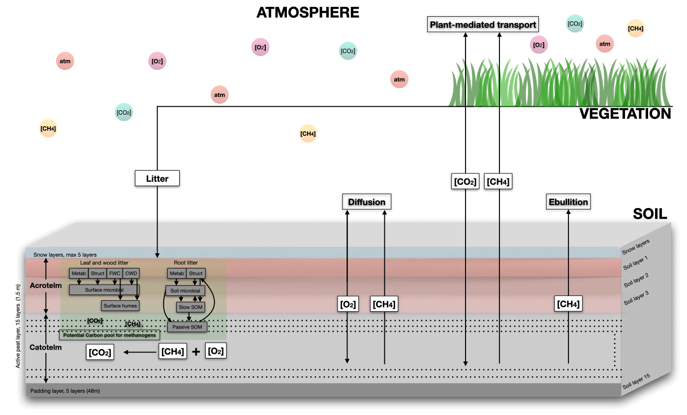
Figure 1 Schematic representation of the CH₄ model in LPJ-GUESS with the CENTURY soil organic model implemented. Carbon for methanogens is allocated to soil layers based on the distribution of roots in each layer. The root density decreases from the top of the peat to the bottom. The assigned carbon in each layer is divided into CH₄ and CO₂. Oxygen (O₂) either directly diffuses or is transported through plants. The availability of O₂ determines the amount of CH₄ in the soil, as it oxidises a fraction of CH₄. Similarly, CH₄ can also either directly diffuse or be transported to the atmosphere in bubbles or it can be transported by vascular plants. The equilibrium between gaseous bubbles of CH₄ and dissolved CH₄ in water is controlled by the maximum solubility of CH₄. Any CH₄ that exists in gaseous form will escape to the atmosphere via ebullition.

The active wetland peat in the LPJ-GUESS is represented by a 1.5 m deep column that is further divided into 15 layers of 0.1 m thickness each (see Fig. 1). The uppermost three layers comprise the acrotelm, within which the water table can vary. The underlying 12 layers of catotelm are permanently saturated with water (Wania et al., 2009a). The decomposed organic carbon on each day (explained in Sect. S1.4) is distributed vertically in different peat soil layers in proportion to an assumed static root distribution (see Eq. 1). This carbon pool is considered to be the “potential carbon pool” for methanogenic archaea and is the basic concept behind the CH₄ model in LPJ-GUESS. The total available carbon is decomposed into two components – CO₂ and CH₄ – depending on the availability of O₂ in the soil. The dissolved CH₄ concentration and the gaseous CH₄ fraction are calculated based on the estimated CH₄ content in each layer. A portion of the estimated CH₄ is oxidised by soil O₂, whereas the remainder is transported to the atmosphere by diffusion, ebullition, or plant-mediated transport. Apart from being the key factor in estimating the potential carbon pool, root biomass in each soil layer also plays a role in the transport of O₂ and CH₄ into and out of each layer, as this transport is mediated by the plants. From different studies of various wetland PFTs, Wania et al. (2010) observed an exponential decrease in the root biomass with depth that was proportional to the degree of anoxia, which is expressed by the following equation, also used in LPJ-GUESS:

$$\begin{array}{}\text{(1)}& f_{\mathrm{root}}=C_{\mathrm{root}}{e}^{z/{\mathit{\lambda }}_{\mathrm{root}}},\end{array}$$

where f_root is the fraction of root biomass at a certain depth z, λ_root=0.2517 m is the decay length, and C_root=0.025 is a normalisation constant. This distribution ensures that approximately 60 % of the roots are distributed within the acrotelm, and the root fraction in the lowest soil layer is adjusted to achieve a total root distribution of 1 across all 15 soil layers.

2.2.1 CH₄ production

Due to its wide range, the ${\mathrm{CH}}_{\mathrm{4}}/{\mathrm{CO}}_{\mathrm{2}}$ ratio from decomposition is challenging to predict. For example, Segers (1998) observed high variation in the CH₄-to-CO₂-production molar ratio of between 0.001 and 1.7 under anaerobic conditions. Hence, it is defined in the model as an adjustable parameter weighted by the degree of anoxia (α): $\mathit{\alpha }=\mathrm{1}-(F_{\mathrm{air}}+f_{\mathrm{air}})$, where F_air is the fraction of air in the soil layers and f_air is the fraction of air in peat (Wania et al., 2009a) (see Sect. S1 for details).

The production of CH₄ on each day in each layer is determined as follows:

$$\begin{array}{}\text{(2)}& {{\mathrm{CH}}_{\mathrm{4}}}_{\mathrm{prod}}=\mathit{\alpha }\left(z\right)\times f_{\mathrm{root}}\left(z\right)\times {\mathrm{CH}}_{\mathrm{4}}/{\mathrm{CO}}_{\mathrm{2}}\times R_{\mathrm{h}},\end{array}$$

where α(z) is the degree of anoxia at depth z, f_root(z) is the fraction of roots in the peat at depth z, ${\mathrm{CH}}_{\mathrm{4}}/{\mathrm{CO}}_{\mathrm{2}}=\mathrm{0.085}$ (prior value in the model) is the tuning parameter for the CH₄-to-CO₂-production ratio, and R_h is the daily heterotrophic respiration. Note that the model is set to ${{\mathrm{CH}}_{\mathrm{4}}}_{\mathrm{prod}}=\mathrm{0}$ when F_water<0.1, assuring no CH₄ production in frozen and/or dry soils (i.e. the model assumes there is no water when the water is frozen and, hence, F_water is 0).

2.2.2 CH₄ oxidation

As mentioned above, the CH₄ fraction that is oxidised (represented by the parameter f_oxid=0.5 as the prior value in the model) depends on the availability of O₂ in the soil. A part of the O₂ transported to the soil will be consumed by the plant roots and non-methanotrophic microorganisms. The remaining part is then used to oxidise CH₄. The oxidised CH₄ is added to the CO₂ pool, and the remainder stays in the CH₄ pool.

2.2.3 Total CH₄ flux

Diffusion, ebullition, and plant-mediated transport are the three pathways via which CH₄ is transported to the atmosphere. The total CH₄ flux from high-latitude wetland patches in the model is represented as follows:

$$\begin{array}{}\text{(3)}& F_{{\mathrm{CH}}_{\mathrm{4}}}={{\mathrm{CH}}_{\mathrm{4}}}_{\mathrm{diff}}+{{\mathrm{CH}}_{\mathrm{4}}}_{\mathrm{plant}}+{{\mathrm{CH}}_{\mathrm{4}}}_{\mathrm{ebul}},\end{array}$$

where ${{\mathrm{CH}}_{\mathrm{4}}}_{\mathrm{diff}}$ is the CH₄ flux component from diffusion, ${{\mathrm{CH}}_{\mathrm{4}}}_{\mathrm{plant}}$ is the CH₄ flux component from plant-mediated transport, and ${{\mathrm{CH}}_{\mathrm{4}}}_{\mathrm{ebul}}$ is the CH₄ flux component from ebullition. As the daily CH₄ production in each layer is dependent on R_h (Eq. 2), $F_{{\mathrm{CH}}_{\mathrm{4}}}$ is subtracted from R_h before saving the daily heterotrophic respiration. Any CO₂ generated, whether from heterotrophic respiration or CH₄ oxidation, is released into the atmosphere.

Diffusion

The fractions of CH₄, CO₂, and O₂ that are transported to the atmosphere and from the atmosphere through diffusion are calculated by solving the gas diffusion equation within the peat layers using a Crank–Nicolson numerical scheme with a time step of 15 min. The molecular diffusivities of these gases in soil depend on temperature, soil porosity, and the water and air content of the soil. Diffusivity in water is derived by fitting a quadratic curve to observed diffusivities at different temperatures, as described in Broecker and Peng (1974); diffusivity in the air and its temperature dependency are derived from the values taken from Lerman (1979); and diffusivity in soil and its temperature dependency are estimated from the Millington–Quirk model, as described in Millington and Quirk (1961). A detailed description can be found in Wania et al. (2010).

At the water–air surface, the gas diffusivities change by a minimum of 4 orders of magnitude; hence, at the water–air boundary, the flux is calculated by the following equation:

$$\begin{array}{}\text{(4)}& J=-\mathit{\psi }\left(C_{\mathrm{surf}}-C_{\mathrm{eq}}\right),\end{array}$$

where C_surf is the surface water gas concentration; C_eq is the concentration of gas in equilibrium with the atmospheric partial pressure, estimated using Henry’s law; and ψ is the gas exchange coefficient, also called the piston velocity, which is usually difficult to estimate for different gases. In this case, the piston velocities of CH₄, CO₂, and O₂ are calculated by relating them to the known piston velocity of SF6 via the following equation:

$$\begin{array}{}\text{(5)}& \mathit{\psi }*={\mathit{\psi }}_{\mathrm{600}}{\left({\displaystyle \frac{Sc*}{\mathrm{600}}}\right)}^n,\end{array}$$

where ${\mathit{\psi }}_{\mathrm{600}}=\mathrm{2.07}+\mathrm{0.215}\times U_{\mathrm{10}}^{\mathrm{1.7}}$ is the piston velocity of SF6 normalised to a Schmidt number of 600 (subjected to the wind speed U₁₀ at 10 m from the ground, which is considered to be 0 in the model), Sc* represents the Schmidt number of the gas under consideration, and $n=-\mathrm{1}/\mathrm{2}$ (see Wania et al., 2010, for details).

As mentioned above the diffusion through the soil is affected by soil porosity, i.e. by the value of F_air(t,z). When F_air≤0.05 in a given soil layer, the diffusivity values of water are used; otherwise (F_air>0.05), the diffusivity values of air, which are 4 orders of magnitude larger than those of water, are used. At each daily time step, before diffusion is calculated, the gas flux J at the boundary is used to update the dissolved gas content. The surface concentration C_surf of CH₄ will mostly be greater than C_eq; hence, J will be negative, denoting a flux to the atmosphere, although it is possible for CH₄ to diffuse into the soil in small amounts if the concentrations at the surface are suitable. The resulting daily flux of CH₄ is determined as the total ${{\mathrm{CH}}_{\mathrm{4}}}_{\mathrm{diff}}$.

Ebullition

Ebullition depends on the solubility of CH₄ at a given temperature and pressure and occurs when the water table reaches the surface during periods of high CH₄ emission. Following Wania et al. (2010), in LPJ-GUESS, the best-fitted curve is represented as follows:

$$\begin{array}{}\text{(6)}& S_{\mathrm{B}}=\mathrm{0.05708}-\mathrm{0.001545}T+\mathrm{0.00002069}{T}^{\mathrm{2}},\end{array}$$

where S_B is the Bunsen solubility coefficient (i.e. the volume of gas dissolved per volume of liquid at atmospheric pressure and a given temperature).

The CH₄ in each layer is converted to a maximum allowable dissolved mass, and this limit is used to separate the CH₄ in the form of dissolved and gaseous components. If there is any CH₄ that exceeds the maximum solubility of a layer, it will be released into the atmosphere. The CH_4ebul is calculated by adding the ebullition fluxes from all layers.

Plant-mediated transport

Plant-mediated transport of CH₄ occurs via the aerenchyma (the gas-filled tissues) of vascular plants, either through concentration gradient or active pumping from the soil to the atmosphere. Only the passive mechanism (through a concentration gradient) is considered in the model, as it is the most dominant one (Cronk and Fennessy, 2016). Abundance, biomass, phenology, and the rooting depth of aerenchymatous plants are considered to calculate this. Only the flood-tolerant C₃ graminoids are considered for plant-mediated gas transport in the model (see Table S2 in the Supplement); hence, plant-mediated transport of O₂ and CH₄ can only occur when C₃ graminoids are present in a simulated patch.

The transport depends on the cross-sectional area of plant tillers (all of the secondary shoots produced by grasses like Poaceae or Gramineae) in each soil layer, assuming that a significantly high percentage of CH₄ is oxidised in the highly oxic zone near the roots, where methanotrophs flourish, before they enter into the plant tissue.

The mass of the tiller is calculated as follows:

$$\begin{array}{}\text{(7)}& m_{\mathrm{tiller}}=b_{\mathrm{graminoid}}\times P\left(\mathrm{leaf}\right),\end{array}$$

where b_graminoid is the leaf biomass of graminoids, and P represents the daily phenology, which is the fraction of potential leaf cover that has reached full development. To calculate the number of tillers (n_tiller), the total weight of tillers (m_tiller) is divided by the average weight of an individual tiller (w_tiller). The cross-sectional area of tillers (A_tiller) can then be obtained as follows:

$$\begin{array}{}\text{(8)}& A_{\mathrm{tiller}}=n_{\mathrm{tiller}}\times {\mathit{\varphi }}_{\mathrm{tiller}}\times \mathit{\pi }{r}_{\mathrm{tiller}}^{\mathrm{2}},\end{array}$$

where r_tiller is the tiller radius and ϕ_tiller is the tiller porosity. Based on the optimisation of McGuire et al. (2012), Tang et al. (2015), and Zhang et al. (2013), the value of r_tiller is estimated as 0.0035 m, and based on Wania et al. (2010), the values of ϕ_tiller and W_tiller are estimated as 70 % and 0.22 gC per tiller, respectively. Each soil layer is allocated a fraction of the total cross-sectional area of tillers based on the root fraction estimated in that layer. The CH_4plant is estimated by adding the plant-mediated CH₄ fluxes from all layers.

2.3 Parameters selected for optimisation

Parameter values related to the processes of CH₄ emission in LPJ-GUESS are mostly adopted from the parameter values described in Wania et al. (2010). As Wania et al. (2010) had difficulties finding the optimal parameter values for many of the parameters, they performed some preliminary analyses for seven uncertain parameters for which there were little or no data available. They performed a simple initial sensitivity test by taking four sets of values for each of the seven parameters, followed by a parameter fitting exercise with three sets of values for each of the seven parameters. They ran the model with all 2187 different combinations for 7 sites for 1 year. As a result, they got an RMSE range of between 226.4 and 18.3 (mg CH₄ m⁻² d⁻¹) for the different sites, which clearly indicates loosely fitted parameters with a high degree of uncertainty.

In this study, parameters for the optimisation are selected based on their sensitivity to the model output (CH₄) and expert opinion. We used a simple method to calculate the percentage difference in output (single simulation) when varying only one input parameter at a time from its permitted minimum value to its maximum (Hoffman and Miller, 1983; Bauer and Hamby, 1991). The “sensitivity index” (SI) is calculated using the following equation:

$$\begin{array}{}\text{(9)}& \mathrm{SI}={\displaystyle \frac{D_{\max }-D_{\min }}{D_{\max }}},\end{array}$$

where D_min and D_max represent the model output values corresponding to the respective minima and maxima of the corresponding parameter range. The values are taken based on expert opinion.

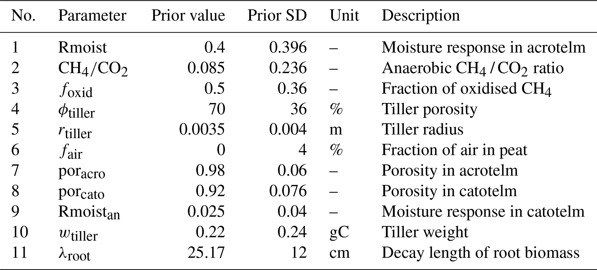
We considered 5 of the 7 parameters that Wania et al. (2010) tested in their sensitivity analysis (2 parameters related to the root exudate decomposition are not used in LPJ-GUESS) as well as 11 other parameters used in LPJ-GUESS. Based on their high SI values, we chose 11 of them for the optimisation (Fig. 2, Table 1).

Among the five eliminated parameters, ag_frac is the fraction of annual net primary production (ANPP) used to calculate number of tillers, DT_min is the minimum temperature (°C) for heterotrophic decomposition, por_org is the porosity of organic material, C_con is the carbon content of biomass, and U₁₀ is the possible constant value of wind speed at 10 m height. Among the selected parameters related to the CH₄ production, Rmoist and Rmoist_an are the response of the soil moisture content to the soil organic matter decomposition in the acrotelm and catotelm, respectively (see Eq. 8 in Supplement); ${\mathrm{CH}}_{\mathrm{4}}/{\mathrm{CO}}_{\mathrm{2}}$ is the CH₄-to-CO₂ ratio under the anaerobic conditions (Eq. 2); f_air is the fraction of air in peat (Sect. 2.2.1 and Eq. 2); por_acro and por_cato are the porosity in the acrotelm and catotelm, respectively (see Sect. S1); and λ_root is the decay length of root biomass in peat (Eq. 1). Among the selected parameters related to the CH₄ transportation, f_oxid is the fraction of oxidised CH₄ (Sect. 2.2.2) related to the CH₄ oxidation, w_tiller is the average weight of an individual tiller, r_tiller is the tiller radius, and ϕ_tiller is the tiller porosity (Eq. 8).

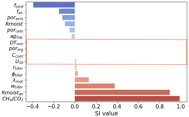
Figure 2 Tested parameters for the optimisation and their SI values. Red and blue colours indicate an increase or decrease in the total CH₄ flux, respectively, when the value of the parameter increases.

Table 1 Selected model parameters for the assimilation. The prior values, units, prior standard deviation (SD), and parameter description are given.

2.4 Parameter optimisation framework

We assumed Gaussian PDFs to depict both the prior distributions of the parameters and the deviation between model and observations. The resulting model can be formulated as follows:

$$\begin{array}{}\text{(10)}& \begin{array}{rl}Y|x& \sim N\left(M\right(x),R),\\ x& \sim N(x_{\mathrm{p}},B).\end{array}\end{array}$$

Here, Y represents the observations; M(x) is the LPJ-GUESS output given parameters x; x_p represents the prior values of the parameters; and R and B are error covariance matrices describing the uncertainty in observations and priors, respectively.

The prior uncertainties (B) are based on expert opinion and were kept relatively large to reduce the prior's influence on the posterior parameter estimates. We have assumed prior variance for each parameters as 40 % of their expected range (see Table 1). The parameters are also assumed to be a prior uncorrelated, due to the lack of good and consistent expert opinions regarding dependence.

2.4.1 Cost function

Using the Bayesian framework, the posterior for the parameters becomes

$$\begin{array}{}\text{(11)}& P\left(x\right|Y)={\displaystyle \frac{P\left(Y\right|x\left)p\right(x)}{p\left(Y\right)}}\propto P(Y\left|x\right)p\left(x\right),\end{array}$$

which, on a log scale, results in the following quadratic cost function (Tarantola, 1987):

$$\begin{array}{}\text{(12)}& \begin{array}{rl}\log P\left(x\right|Y)& =-J\left(x\right)+\text{const.}\\ J\left(x\right)& ={\displaystyle \frac{\mathrm{1}}{\mathrm{2}}}(Y-M(x\left){)}^t{R}^{-\mathrm{1}}\right(Y-M\left(x\right))\\ & +{\displaystyle \frac{\mathrm{1}}{\mathrm{2}}}(x-x_{\mathrm{p}}{)}^t{B}^{-\mathrm{1}}(x-x_{\mathrm{p}}),\end{array}\end{array}$$

where “const.” represents normalising constants not depending on the unknown parameters. The two terms in J(x) represent model–data misfit and the prior information on the parameters. A number of experiments aim to achieve the smallest cost function values to locate the optimal parameter set within the parameter space.

2.5 Adaptive Metropolis–Hastings (MH) algorithm

To search for the optimal posterior parameters, we used an MCMC-MH algorithm (Metropolis et al., 1953a; Hastings, 1970a). A standard MH algorithm generates samples from a target distribution by, in each iteration, drawing from a proposal distribution and then either accepting the new state or copying the old state. For a Gaussian random walk, proposals ($\widehat{x}$) are generated by adding a mean-zero normal random variable to the current value (x_t):

$$\begin{array}{}\text{(13)}& \widehat{x}=x_t+\mathit{ϵ},\mathit{ϵ}\sim N(\mathrm{0},\mathit{\lambda }\mathrm{\Sigma }),\end{array}$$

where λΣ is a scaling and covariance matrix describing the spread of the added random variable. The new value is accepted with a probability that compares the likelihood (or cost function) of the proposed and old sample:

$$\begin{array}{}\text{(14)}& \mathit{\alpha }=min\left(\mathrm{1},{\displaystyle \frac{P\left(\widehat{x}\right|Y)}{P\left(x_t\right|Y)}}\right)=min\left(\mathrm{1},\exp (-J(\widehat{x})+J(x_t\left)\right)\right).\end{array}$$

If the value is accepted, set $x_{t+\mathrm{1}}=\widehat{x}$, otherwise keep the previous value, $x_{t+\mathrm{1}}=x_t$. The resulting sequence of states will represent dependent samples from the target distribution.

The adaptive MH algorithm used here contains three key concepts that are explained in the following sections: transformed proposals, providing a natural way of including limits on the parameters; the adaptive random walk, allowing the algorithm to estimate λ and Σ from the target distribution; and tempering of the target distribution, to reduce the effects of local maxima and allow better exploration of the target.

2.5.1 Transformed proposals

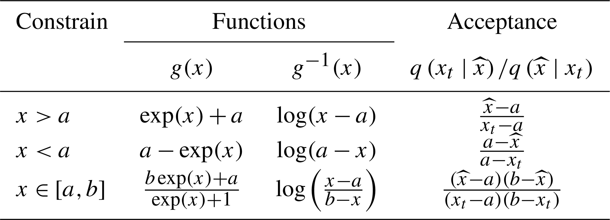
The standard proposal in Eq. (13) does not include any restrictions on the parameters. To handle parameter limits, we transformed the parameters, resulting in an adjusted random walk proposal:

$$\begin{array}{}\text{(15)}& \begin{array}{rl}{z}_t& =g^{-\mathrm{1}}\left(x_t\right),\\ \widehat{z}& =z_t+\mathit{ϵ},& \mathit{ϵ}& \sim N(\mathrm{0},\mathit{\lambda }\mathrm{\Sigma }),\\ \widehat{x}& =g\left(\widehat{z}\right).\end{array}\end{array}$$

A list of possible limits and corresponding functions are given in Table 2. Note that different functions can be applied to each parameter in x.

Having a transformed proposal requires an adjustment of the acceptance probability (Hastings, 1970a) in Eq. (14) to

$$\begin{array}{}\text{(16)}& \begin{array}{rl}\mathit{\alpha }& =min\left(\mathrm{1},{\displaystyle \frac{p\left(\widehat{x}\right|Y)}{p\left(x_t\right|Y)}}\prod _i{\displaystyle \frac{q\left(x_t^{\left(i\right)}\mid {\widehat{x}}^{\left(i\right)}\right)}{q\left({\widehat{x}}^{\left(i\right)}\mid x_t^{\left(i\right)}\right)}}\right)=\\ & =min\left(\mathrm{1},\exp (-J(\widehat{x})+J(x_t)\right.\\ & \left.+\sum _i\log \left({\displaystyle \frac{q\left(x_t^{\left(i\right)}\mid {\widehat{x}}^{\left(i\right)}\right)}{q\left({\widehat{x}}^{\left(i\right)}\mid x_t^{\left(i\right)}\right)}}\right)\right).\end{array}\end{array}$$

Here, $x_t^{\left(i\right)}$ denotes the ith parameter in the x_t vector, and the q terms are given in Table 2. Note that each transformation results in one adjustment for that parameter and that all adjustments have to be multiplied together.

Table 2 Summary of transformations and corresponding adjustments to the acceptance probability for the three cases of variables with a lower limit, variables with an upper limit, and variables constrained to an interval.

2.5.2 Adaptive random walk

It has been shown that the optimal MH algorithm behaviour is obtained when about 20 %–30 % of samples are accepted (Gelman et al., 1996; Roberts et al., 1997). For the proposal in Eq. 13, this is achieved when Σ corresponds to the posterior covariance matrix of the target distribution, P(x|Y), and the scaling is $\mathit{\lambda }={\mathrm{2.38}}^{\mathrm{2}}/d$, where d is the number of parameters in x. The key idea of the adaptive algorithms suggested in Andrieu and Thoms (2008) is to recursively estimate both Σ and λ from previous samples. An important note for the transformed proposal in Eq. (15) is that Σ and λ relate to the transformed variable z_t and not x_t.

A Rao-Blackwellised update of the covariance matrix will consider both the proposal, $\widehat{z}$, and the previous value, z_t, weighted according to the acceptance probability, α, computed in Eq. (16). The expectation and covariance matrix are updated recursively as follows:

$$\begin{array}{}\text{(17a)}& {\displaystyle }{\mathit{\mu }}_{t+\mathrm{1}}=(\mathrm{1}-{\mathit{\gamma }}_{t+\mathrm{1}}){\mathit{\mu }}_t+{\mathit{\gamma }}_{t+\mathrm{1}}\left(\mathit{\alpha }\widehat{z}+(\mathrm{1}-\mathit{\alpha })z_t\right),\text{(17b)}& {\displaystyle }\begin{array}{rl}{\mathrm{\Sigma }}_{t+\mathrm{1}}& =(\mathrm{1}-{\mathit{\gamma }}_{t+\mathrm{1}}){\mathrm{\Sigma }}_t+{\mathit{\gamma }}_{t+\mathrm{1}}[\mathit{\alpha }\left(\widehat{z}-{\mathit{\mu }}_{t+\mathrm{1}}\right){\left(\widehat{z}-{\mathit{\mu }}_{t+\mathrm{1}}\right)}^{\top }\\ & +(\mathrm{1}-\mathit{\alpha })\left(z_t-{\mathit{\mu }}_{t+\mathrm{1}}\right){\left(z_t-{\mathit{\mu }}_{t+\mathrm{1}}\right)}^{\top }],\end{array}\end{array}$$

where γ_t is an adaptation factor and we have used ${\mathit{\gamma }}_t=t^{-\mathrm{0.51}}$.

The global adaptive scaling then updates the scaling factor λ as follows:

$$\begin{array}{}\text{(18)}& {\displaystyle }\log {\mathit{\lambda }}_{t+\mathrm{1}}=(\mathrm{1}-{\mathit{\gamma }}_{t+\mathrm{1}})\log {\mathit{\lambda }}_t+{\mathit{\gamma }}_{t+\mathrm{1}}\left(\mathit{\alpha }-{\mathit{\alpha }}_{\text{target}}\right).\end{array}$$

The update is on a log scale to ensure that λ_t stays positive; the second part of the equation compares the current acceptance probability with a target probability, α_target=0.234, and adjusts λ_t to obtain this desired overall acceptance probability.

To limit the effect of initial values, we first ran 5000 steps of the chain without adaptation and with Σ as 10⁻³ times an identity matrix (i.e. very small initial steps). Thereafter, a covariance matrix Σ was estimated based on the initial samples, and the chain was run for a further 15 000 steps adapting only λ and not Σ. Finally, for the last 80 000 steps, both λ and Σ were updated as described in Andrieu and Thoms (2008). We call the resulting framework the global Rao-Blackwellised adaptive metropolis (GRaB-AM) algorithm.

2.5.3 Tempering the target distribution

For large numbers of data, the cost function J(x) can have very deep local minima, causing the MH algorithm to get stuck, even with the two already outlined adjustments. To reduce the scale of the cost function, we temper the target distribution (Jennison, 1993).

$$\begin{array}{}\text{(19)}& {\displaystyle }\stackrel{\mathrm{̃}}{P}\left(x\right|Y)=P(x|Y{)}^{\mathrm{1}/T}=\exp (-J\left(x\right)/T),\end{array}$$

where T is a suitably large value.

Having run an MH algorithm for N samples, the first N_b samples are discarded as “burn-in”, and expectations or variances can be computed as averages of the remaining samples.

However, with a tempered target distribution, we have samples from $\stackrel{\mathrm{̃}}{P}\left(x\right|Y)$ and need to use importance sampling to adjust for the difference in distributions (Jennison, 1993), resulting in weighted averages

$$\begin{array}{c}{\displaystyle }E\left(x\right|Y)\approx \sum _{i=N_{\mathrm{b}}}^N{w}_i{x}_i,\\ {\displaystyle }V\left(x\right|Y)\approx \sum _{i=N_{\mathrm{b}}}^N{w}_i(x_i-E\left(x\right|Y){)}^{\mathrm{2}},\end{array}$$

where the weights are given by

$$w_i={\displaystyle \frac{\exp \left(-\frac{T-\mathrm{1}}{T}\left(J\right(x_i)-J_{\text{min}})\right)}{{\sum }_{i=N_{\mathrm{b}}}^N\exp \left(-\frac{T-\mathrm{1}}{T}\left(J\right(x_i)-J_{\text{min}})\right)}}$$

and $J_{\text{min}}={min}_{i}J\left(x_i\right)$. The subtraction by J_min is for numerical stability to avoid cases of 0/0 when all J(x_i) are very large. For the case of no tempering, i.e. T=1, the weights simplify to $w_i=\mathrm{1}/(N-N_{\mathrm{b}})$, resulting in unweighted averages.

2.6 Experimental design

We have designed a set of twin experiments and a real-data experiment. For both the twin and real-data experiments, we generated MCMC chains with a length of 100 000 samples, as mentioned in Sect. 2.5.2. MCMC approaches are computationally intensive and time-consuming. In this study, each model simulation took approximately 9 s to complete (using an AMD Ryzen Threadripper processor). As a result, for the 100 000 iterations, it consumed nearly 250 computational hours. However, it should be noted that this study involves the model running for a single site, and the computational speed is highly dependent on the performance of the processors being used.

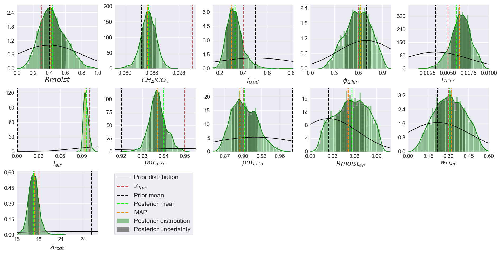
Figure 3 An example of posterior PDFs from the twin experiment. Prior and posterior distributions are illustrated with solid black and solid green lines, respectively. True parameter values (Z_true), the prior mean, the posterior mean, and the MAP are shown in red, black, lime, and orange colours, respectively.

Twin experiment

Twin experiments are designed to assess the performance of the developed GRaB-AM and its ability to recover the parameter values. The daily CH₄ output simulated by LPJ-GUESS using randomly chosen true parameter values (Z_true) within their permitted range of variation is used as the synthetic observation. As the synthesised observation conforms completely to the model, any potential errors in the model have not influenced the parameter optimisation process, ensuring unbiased posteriors. The observations have been assigned uncertainties to resemble the real-data experiment, as described below. It is expected that the assimilated parameters will converge to the true values as the MCMC chain progresses in time. To freely recover the Z_true values, the prior parameter values (x_p) in the cost function (Eq. 12) are set as Z_true. Two scenarios are considered for the twin experiment to test the identifiability of the parameters under different conditions: scenario 1, which has a shorter temporal scale from 2005 to 2014 (10 years), and scenario 2, which has a longer temporal scale from 1901 to 2015 (115 years). Scenario 1 is more realistic and is chosen to mimic the real data at Siikaneva, whereas scenario 2 constitutes an ideal, hypothetical case with observations over the entire simulation period. In each set of the scenarios, the optimisation started from a different initial point in the parameter space that was randomly selected from their prescribed ranges.

Real-data experiment

To estimate the posterior parameter values, an experiment using the real observation from Siikaneva is designed. The observed daily averages are compared with the model simulation in the cost function only when more than 90 % of the hourly observation are available each day. When there are gaps in the daily observation, we eliminate them and their corresponding modelled values from the cost function calculation. In principle, the error covariance matrix R should include both observation uncertainties and their correlations. As the latter is difficult to estimate, we neglected them, and the observation uncertainties are estimated as 30 % for the daily observations greater than 0.01 gC m⁻² d⁻¹ and a floor value of 0.3 for the observations less than 0.01 gC m⁻² d⁻¹.

2.7 Parameter value estimation

For all of the experiments conducted in this study, the first 75 % of the GRaB-AM chains are discarded as the burn-in. The PDFs generated after the burn-in are used to estimate each parameter's maximum a posteriori probability (MAP), posterior mean, and standard deviation (SD). Following the idea used in Braswell et al. (2005), the parameter distributions are grouped into three categories: “well-constrained”, “poorly constrained”, and “edge-hitting” parameters. The well-constrained parameters are those that exhibit a well-defined unimodal distribution with a low SD. The poorly constrained parameters are those that exhibit a relatively flat multi-modal distribution with a large SD. To be more precise with the estimation, for posterior parameter distributions that appeared multi-model, if the SD of the distribution was greater than 20 % of the total range, we classified them as poorly constrained. The edge-hitting parameters are those that cluster near one of the edges of their prior range.

2.8 Posterior resampling experiment

To examine the effect of parameter optimisation on flux components, we designed a resampling experiment from the posterior parameter distributions. From the experiment conducted using site observations, 1000 sets of parameters were randomly selected and used to run the model to simulate the CH₄ flux components. The outputs from each simulation of the experiment were used to analyse the process correlations and process–parameter relationships.

3 Results

3.1 Twin experiment using GRaB-AM

We ran a set of four different twin experiments for each of the scenarios mentioned in Sect. 2.6. Each of them shows a reasonably good convergence, regardless of their chosen initial values. In scenario 1, all parameters except for ${\mathrm{CH}}_{\mathrm{4}}/{\mathrm{CO}}_{\mathrm{2}}$ and λ_root showed good convergence (see Fig. S1 in the Supplement; posterior parameter correlations of the first experiment shown in Fig. S1 are provided in Fig. S2). The results of scenario 2 are not shown, as they followed the same pattern. The resulting PDFs of experiment 1 in scenario 1 after the burn-in are represented in Fig. 3, which shows the mean and MAP values as well as the SD of the parameters. The parameter values and related statistics are given in Table 3.

The parameter retrieval capacity of the GRaB-AM algorithm is estimated as the “retrieval score” by dividing the posterior mean estimates of the parameters from all of the chains in each scenario by the Z_true parameter values. The idea behind the retrieval score is that, in an ideal case of complete recovery, the posterior parameter estimate and the Z_true value are the same; hence, the retrieval score would be 1. Figure 5 shows the retrieval scores obtained for each parameter and their 1σ value. In scenario 1, the ϕ_tiller, por_acro, por_cato, w_tiller, and λ_root are well retrieved with a low SD. Scenario 2 performed better in parameter retrieval compared with scenario 1. In scenario 2, the majority of the parameters except the ${\mathrm{CH}}_{\mathrm{4}}/{\mathrm{CO}}_{\mathrm{2}}$, r_tiller, w_tiller, and λ_root showed good retrieval scores but with comparatively high SDs (see Fig. 5). The overall mean retrieval score estimation is based on the ratio of the estimated and true values, given a value of 0.95 with an SD of 0.19 for scenario 1 and a value of 1 with an SD 0.21 for scenario 2 (see Fig. 5).

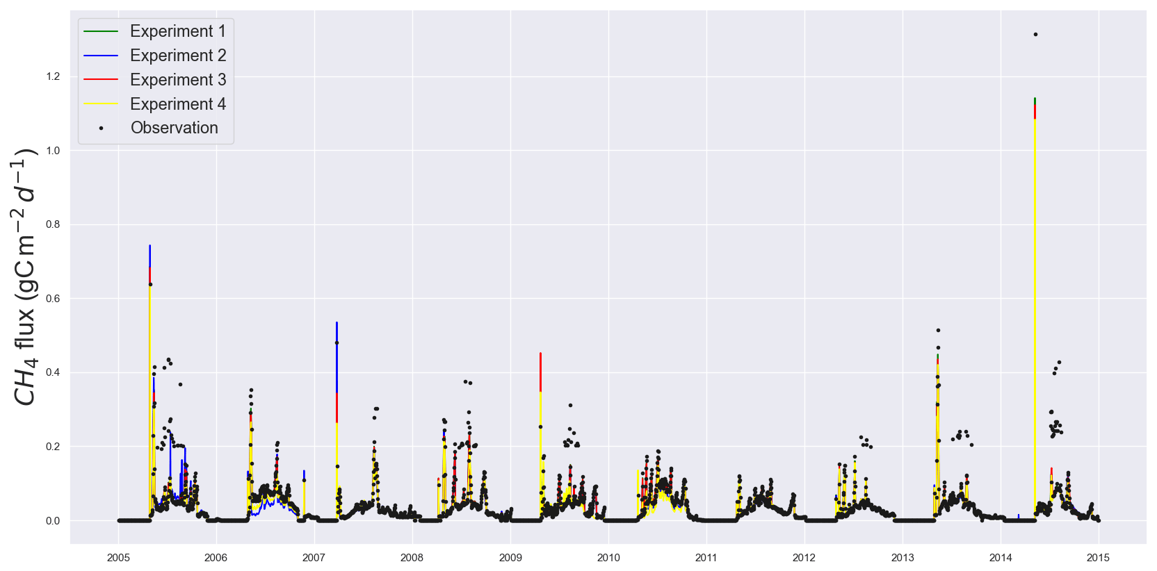
Figure 4 Time series estimates of the twin experiments in scenario 1. The simulations, using four sets of posterior parameter values obtained from the twin experiments, are plotted against the twin observation used.

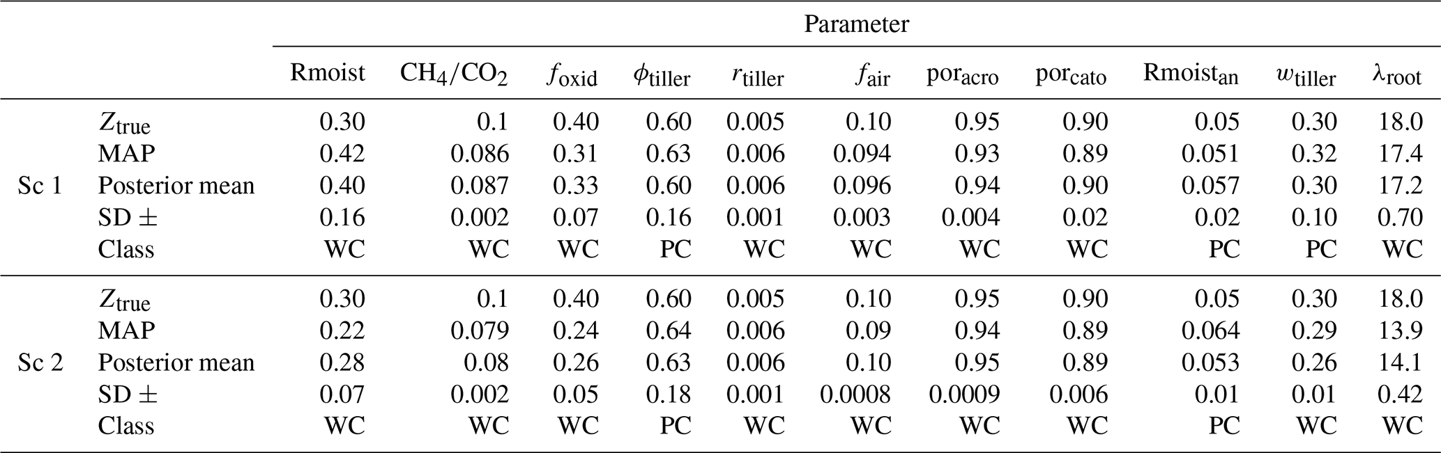
Table 3 The posterior mean, MAP, and SD of retrieved parameters for selected twin experiments in scenario (Sc) 1 and 2 and the parameter classes estimated from analysing the distributions of all four chains. The parameter classes include well-constrained (WC) and poorly constrained (PC) parameters.

In general, the twin experiments have resulted in well-constrained and poorly constrained parameter classes. Examples of the different classes of the distributions for experiment 1 of scenario 1 are shown in Fig. 3. Based on the posterior distributions estimated from all four GRaB-AM chains, the parameters Rmoist, ${\mathrm{CH}}_{\mathrm{4}}/{\mathrm{CO}}_{\mathrm{2}}$, f_oxid, r_tiller, f_air, por_acro, por_cato, and λ_root are well constrained in scenario 1, whereas the parameters Rmoist, ${\mathrm{CH}}_{\mathrm{4}}/{\mathrm{CO}}_{\mathrm{2}}$, f_oxid, r_tiller, f_air, por_acro, por_cato, w_tiller, and λ_root are well constrained in scenario 2 (see Table 3).

Table 4 Cost function reduction observed in scenario (Sc) 1 and 2 of the twin experiments. The prior and posterior cost function values obtained from four sets of experiments for each scenario are provided. The misfit between observed and expected (zero) cost function values are represented as the reduced χ² value.

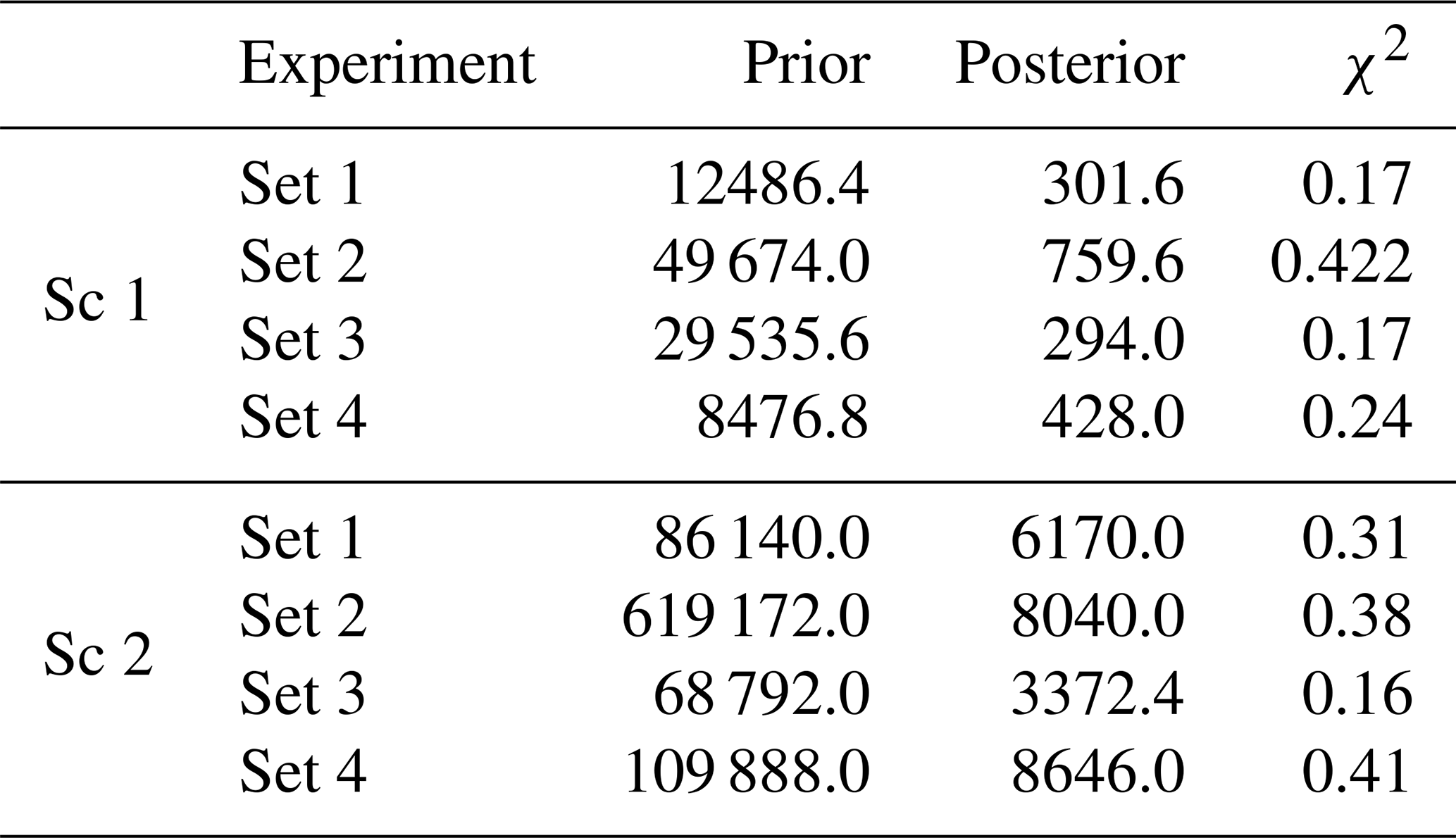
The reduced posterior cost function values and their χ² values are given in Table 4. Here, the reduced χ² values are calculated by dividing twice the cost function by the number of observations used in the assimilation. Overall, the χ² values indicate a statistically robust reduction in the cost function in all of the experiments, although a systematic behaviour of being below 1 is observed.

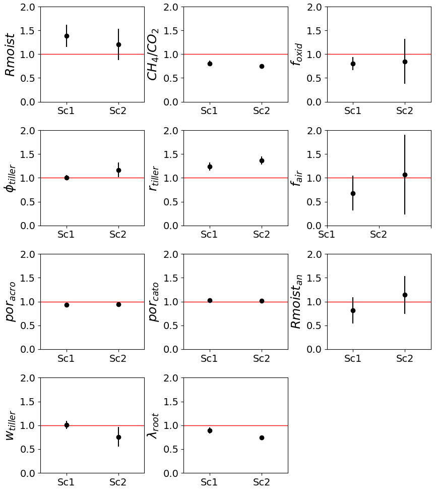
Figure 5 Twin experiment results in terms of the mean retrieval score based on the ratio of the estimated and Z_true values of the parameters. The horizontal red lines indicate a complete retrieval, and the error bar shows the SD obtained from different chains in different scenarios. Sc1 and Sc2 indicate the two respective scenarios.

3.2 Real-data experiments and optimised parameters

For the experiment with the real data, the observations collected at the Siikaneva wetland are assimilated using the GRaB-AM algorithm. The MCMC trace plots are exemplified in Fig. 6.

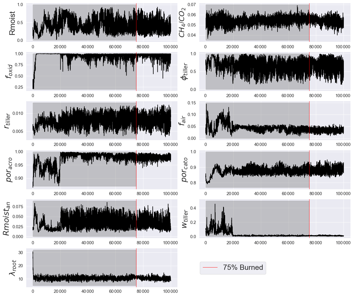
Figure 6 An example of the GRaB-AM chains for the experiment with real observations showing all 100 000 values in the chain. The first 75 % of values were discarded as burn-in and are greyed out in the figures. The remaining 25 % (from the red vertical lines) of values were used for the analyses.

3.2.1 Optimised parameter values and distributions

The posterior parameter PDFs are shown in Fig. 7. In contrast to the twin experiments, the parameters fell into three categories: well-constrained, poorly constrained, and edge-hitting parameters. The classifications are given in Table 5. The PDFs for the Rmoist, ${\mathrm{CH}}_{\mathrm{4}}/{\mathrm{CO}}_{\mathrm{2}}$, ϕ_tiller, f_air, por_acro, w_tiller, and λ_root parameters are classified as well-constrained distributions; the PDFs for r_tiller, por_cato, and Rmoist_an are classified as poorly constrained distributions; and that for f_oxid is classified as an edge-hitting distribution. In both the well-constrained and poorly constrained parameters, high kurtosis is observed. The values of f_oxid, which is the edge-hitting parameter, lay near the higher bound of the edges of the prior range, and most of the retrieved values were clustered near this edge. This parameter also exhibited large positive kurtosis and negative skewness. The posterior parameter values and their 1σ SDs along with the prior values are shown in Table 5. The MAP and posterior mean estimates agree on the value for the ${\mathrm{CH}}_{\mathrm{4}}/{\mathrm{CO}}_{\mathrm{2}}$, f_air, and por_acro parameters. For f_oxid, ϕ_tiller, and r_tiller, both the MAP and posterior mean estimates stayed out of one-third of the 1σ range of the posterior distribution, which we consider a large difference. For the remaining parameters, the MAP and posterior mean estimates stayed within one-third of the 1σ of their posterior distribution; hence, we consider this a small difference. For the Rmoist and ${\mathrm{CH}}_{\mathrm{4}}/{\mathrm{CO}}_{\mathrm{2}}$ parameters, the posterior values appeared close to but below the prior values. The posterior values of Rmoist_an appeared very close to but above the prior values. For the ϕ_tiller parameter, the MAP estimate appeared very close to but above the prior value, whereas the posterior mean estimate appeared very close to but below the prior value. For these four parameters, the posterior mean stayed within one-third of the 1σ range of the assumed prior uncertainty. The posterior values of the f_oxid, r_tiller, and f_air parameters appeared slightly above the prior values but outside of one-third of the 1σ range of the prior uncertainty. The prior and posterior values of the por_acro parameter remained the same. In contrast, the por_cato, w_tiller, and λ_root parameters appeared very distant from and below the prior values, out of one-third of the 1σ range of prior uncertainty, but stayed within the prior range (see Sect. 4.2 for details).

3.2.2 Posterior parameter correlation

The 2-D distributions of the posterior parameters and their correlations are illustrated in Fig. 9. Overall, the majority of the parameters showed weak positive or negative correlations with a few exceptions with extreme correlations (the values and corresponding colour code in the triangle above depict this). For example, Rmoist_an showed a high negative correlation with Rmoist, and por_acro showed a high positive correlation with f_air. The 2-D marginal distributions (scatterplots), illustrated in the lower triangle, showed a general tendency toward high clustering within the 1σ range for all of the parameters; in general, the 1-D histograms (on the diagonal; also shown in Fig. 7) appeared as well-constrained unimodal distributions. For further details, the reader is referred to Sect. 4.2.1.

3.2.3 Cost function reduction

The prior and posterior cost function values corresponding to the prior and posterior parameter values are listed in Table 5. The prior cost function value calculated with the default model parameters showed a high-cost value of 48424.4, with a model overestimation of around 4 times the observed flux. After the optimisation, the cost function value was reduced to 2959.8 (reduced χ²=3.82) with the MAP estimate of parameters and to 3002.6 (reduced χ²=3.88) with the posterior mean estimate of parameters.

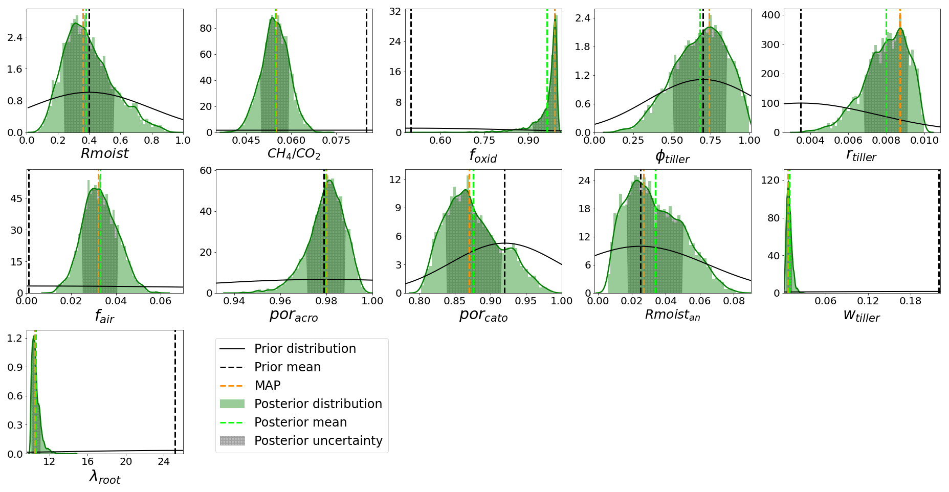
Figure 7 Posterior PDFs of parameters from the GRaB-AM real-data experiment. The green curves shown are the smoothed Gaussian kernel estimates of the posterior distribution on the posterior histograms, whereas the black curves are the prior distributions. The dotted vertical black, lime, and orange lines represents the prior mean, posterior mean, and MAP, respectively. The shaded green area of the distributions represents the 1σ error estimate of the PDFs.

Figure 8 Schematic summery of the resampling experiment. Panel (a) shows the process–parameter correlation and regression slope. Three different flux components of CH₄ as well as the total flux are labelled on the vertical axis, whereas the parameters are labelled on the horizontal axis. The different colours of the circles represent the regression slopes (β) scaled between −1 and 1 (in 11 steps). The blue colour indicates a steeper negative slope (and hence a strong decrease) in CH₄ fluxes with the increasing parameter value, whereas the red colour indicates steeper positive slopes (and hence a strong increase) in CH₄ fluxes with the increasing parameter value. The coefficient of determination (R²) scaled between 0.05 and 1 (in 11 steps) is represented by the size of the circles, with larger circles indicating higher R² values. Panel (b) shows the process–process correlations. Numeric labels on the upper triangle correspond to Pearson's correlation coefficient values. The diagonal of the matrix shows the 1-D histogram for each flux component and the total flux. The 2-D marginal distributions of the sum of the processes and total flux are represented in the lower triangle with contours to indicate the 1σ, 2σ, and 3σ confidence levels. The black dots in the plots indicate the sums of flux components. Ranges of the distributions are labelled on the left and bottom of the panel.

3.2.4 Flux components of the CH₄ simulation and parameter values

To understand how and the magnitude to which each optimised parameter influences the flux components and the total flux, the result of the resampling experiment (see Sect. 2.8) is examined using correlation and regression analyses. The Pearson correlation coefficients and regression slopes are calculated for all 1000 parameter sets and their corresponding sums of the flux components and total flux. Figure 8a shows a schematic summary of the correlation coefficients and regression slopes between the 11 parameters, the flux components, and the total flux. For both the total flux and diffusion, all parameters, except f_oxid and ϕ_tiller, showed a similar regression pattern, although with slight differences in magnitude. This similarity is not surprising, as diffusion is the most dominant among the process components. The total flux showed the highest correlations with ${\mathrm{CH}}_{\mathrm{4}}/{\mathrm{CO}}_{\mathrm{2}}$ and λ_root and the lowest correlation with f_oxid. A detailed discussion of the process–parameter relations can be found in Sect. 4.2.1.

Table 5 Parameter values estimated after the GRaB-AM real-data optimisation. The prior values, MAP, posterior mean, posterior SD, and parameter classes are shown. The parameter classes include well-constrained (WC), poorly constrained (PC), and edge-hitting (EH) parameters. The cost function values corresponding to the parameter values obtained with the prior, MAP, and posterior mean estimates are also shown.

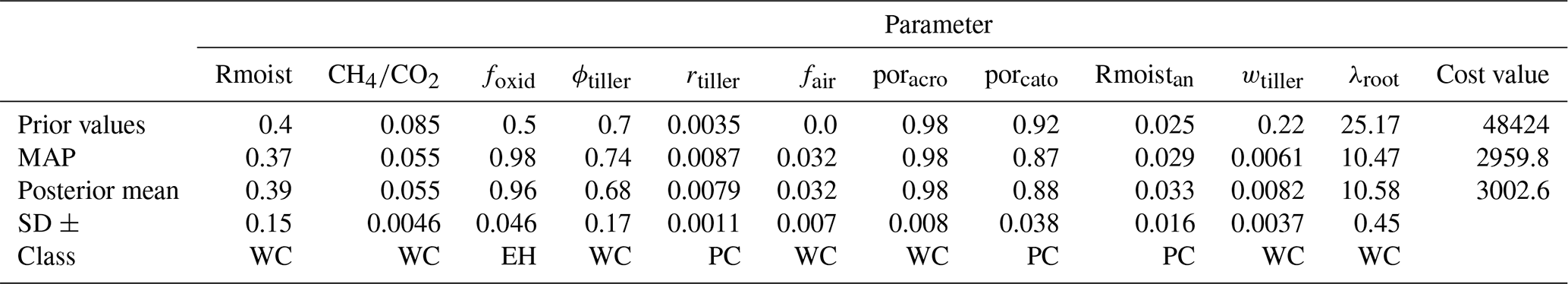
Figure 8b shows the correlations between the sums of flux components resulting from the resampling experiment. The 2-D distributions in the lower triangle show a strong positive relation between diffusion and total flux. Almost all of the parameter residuals are observed within 3σ deviation without many outliers. Except for the correlation between diffusion and total flux, the analysis showed no other strong positive or negative correlations between the components, as can be seen in the correlation plot illustrated in the top triangle of the aforementioned figure panel.

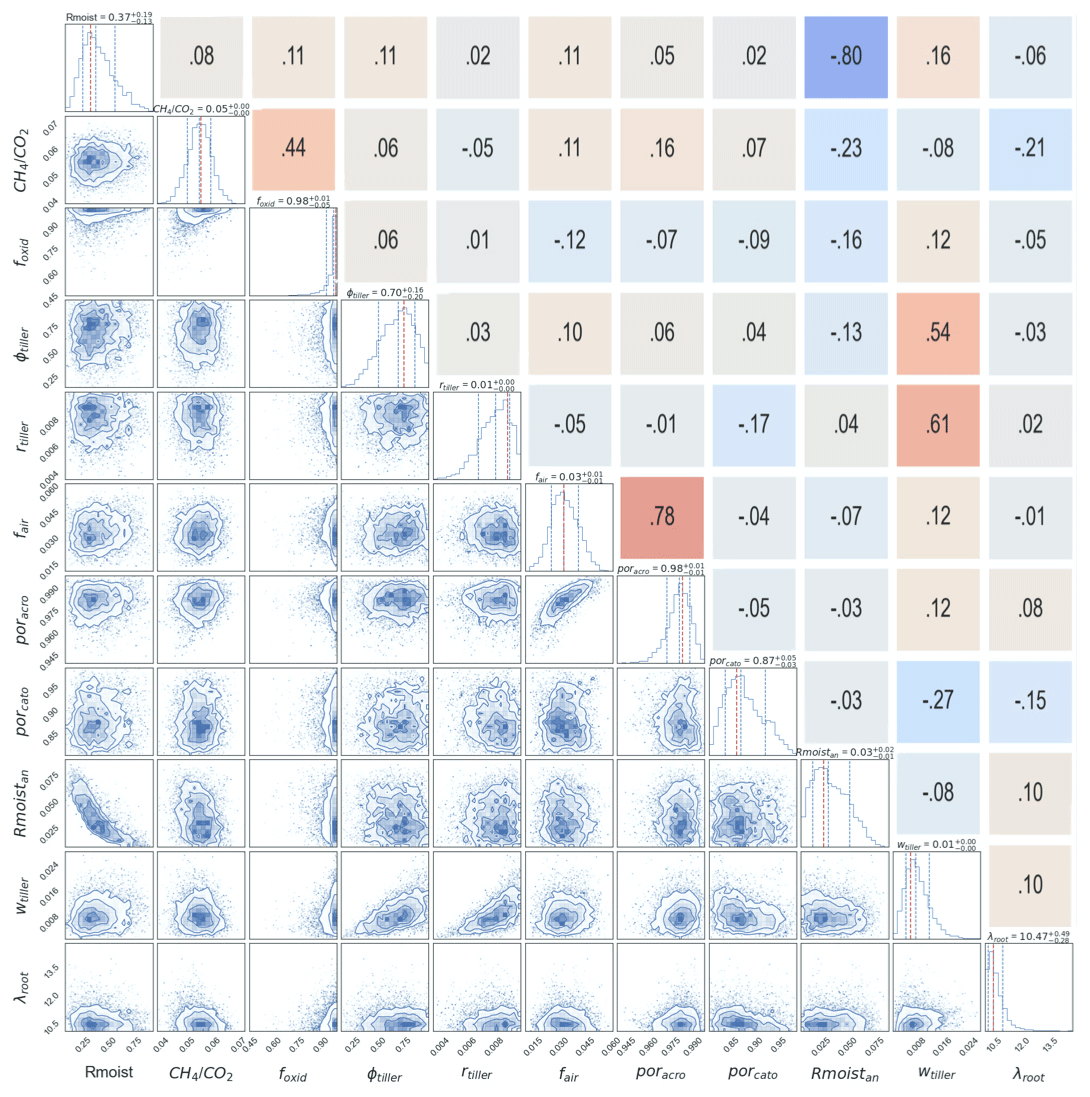
Figure 9 A posteriori correlations between the parameters from the GRaB-AM real-data optimisation. The blue and red colours in the upper triangle represent strong negative and positive correlations, respectively. The numerical labels on the upper triangle are the Pearson's correlation coefficient values. The panels on the diagonal show the 1-D histogram for each model parameter with a dashed red vertical line to indicate the mode. The vertical blue lines are the 0.16, 0.5, and 0.84 quantiles of the distributions. The lower triangle represents the 2-D marginal distributions of each parameter with contours to indicate the 1σ, 2σ, and 3σ confidence levels, whereas the blue dots on the marginal distributions are the posterior parameter values. The ranges of the distributions are labelled on the left and bottom of the figure.

Yearly variations in the fractional contributions of flux components simulated using prior and posterior parameter estimates are examined to understand the impact of the optimisation on the composition of the inter-annual emissions. The time series of the annual sums of flux components as a function of their total flux (in %) are shown in Fig. 10a. The result shows that, among the flux components, diffusion contributes the most to the total CH₄ flux both in prior and posterior estimates, with a slightly higher contribution in the posterior estimate, followed by plant-mediated transport (see Sect. 4.2.3 for detailed discussion).

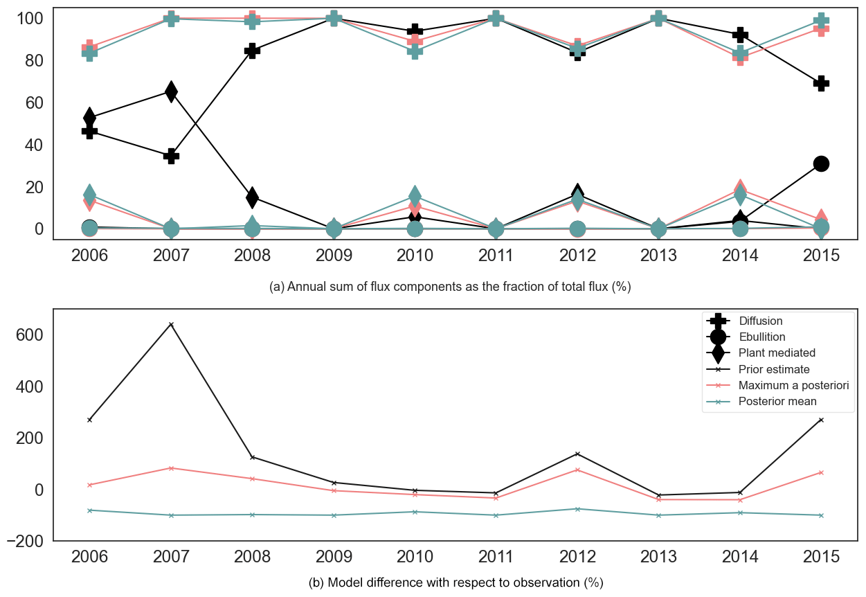
Figure 10 Flux component fractions and the model–data difference (in %). Panel (a) shows the proportions of annual flux components plotted as a function of the total yearly flux. The different flux components are represented with solid lines of different colours, and the symbols on the lines correspond to each flux component. Panel (b) shows the annual model–observation mismatch (in %) with respect to the yearly total CH₄ observation.

The time series model–observation mismatch of prior and posterior estimates for the annual total fluxes can be seen in Fig. 10b; the values are displayed as a percentage of the observed CH₄ flux. The prior estimate showed a mismatch of around 600 % for the first 2 years. Furthermore, a considerably high mismatch is observed in the years 2011, 2012, and 2014. The MAP estimate remained near 0, while the posterior mean estimate exhibited slightly negative values, indicating an underestimation of the flux. Interestingly, the MAP followed the same pattern as the prior estimation by showing an increase whenever the prior increased and a decrease whenever the prior decreased; however, the posterior mean estimate did not show this relation.

The percentage fractions of the annual errors in the flux components are shown in Fig. 11. The effect of optimisation on the individual contributions of each component can be seen from the annual means (solid dots) of their fractional contribution to the total flux. Among the prior estimates of flux components, the prior plant-mediated transport showed the largest error (22.5 %), whereas the ebullition showed the smallest error (9.1 %). In the MAP estimate, ebullition showed the highest error, with a value of 12.3 %, followed by diffusion and ebullition, with similar error values of 6.9 % and 6.8 %, respectively. For the estimate using posterior mean values, diffusion and plant-mediated transport showed around the same errors, 7.5 % and 7.4 %, and ebullition showed the least error (2.6 %). On the right-hand side of the aforementioned figure, the fourth column displays the mean and errors for the inter-annual variation in the total fluxes obtained by prior parameter values and posterior estimates. The prior total estimate showed an error of 4.2 %, while the mean and MAP showed an error of 0.66 % and 0.72 %, respectively.

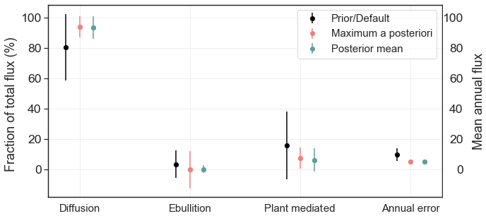
Figure 11 The first three columns of the figure show the fractions of the annual fluxes from process components of the total fluxes. The vertical solid lines represent the 1σ error bars of each component, whereas the dots represent the mean of the annual fluxes. The fourth column (which corresponds to the right y axis) shows the annual mean and annual errors for the inter-annual variation in the total fluxes.

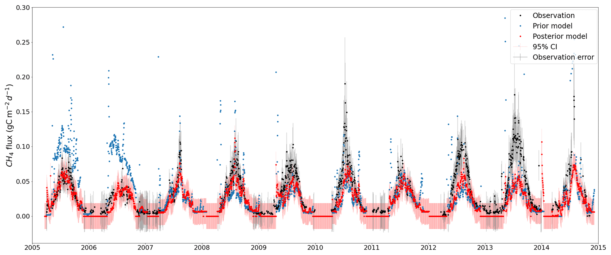
Figure 12 Total CH₄ simulation from the LPJ-GUESS model (red dots) after optimising with the GRaB-AM algorithm. The black dots are the real CH₄ observations from Siikaneva with prior observation error (grey shading). The light red shading around the posterior model simulation is the 95 % confidence interval (CI) of the simulations. The blue dots are the prior simulation with the prior default model parameters. A few outliers above 0.3 gC m⁻² on the vertical axis have been removed from the figure for better visualisation. While most of the observations fall within the confidence intervals, it is important to note that the effects of parameter variations in the posterior are part of these confidence intervals.

3.3 Fit to the observation

Figure 10b illustrates the percentage model–data misfit, and Fig. 12 shows the time series of the assimilated observations as well as the model prior and posterior estimates with their uncertainties. The total RMSE estimated between the prior and observations was 0.044 gC m⁻² d⁻¹, which was reduced to a value of 0.023 gC m⁻² d⁻¹ for the posterior case. This result indicates that most of the mismatch between the prior model estimates and observations was contributed by the large overestimation in the initial years. This overestimation disappeared in the posterior, showing a better agreement with the observation. There are years for which the observations show large peaks during the summer (such as 2010, 2012, and 2013), and the posterior estimates succeeded in capturing these peaks to a large extent, although not completely (see Sect. 4.5 for details).

4 Discussion

4.1 Twin experiment

A common problem with the adaptive MH algorithm is its inability to widely explore the target distribution if the set-up is not well tuned. This can then result in a poor approximation of the target distribution and, hence, poor adaptation. The resulting trace plots shown in Figs. 6 and S1 depict a set of well-explored parameters in their permitted space ranges during the progression of the random walk, indicating a well-tuned assimilation set-up. The use of adaptive Rao-Blackwellised learning of the posterior distribution appeared beneficial during the transients of the chains whenever the acceptance probability was dropped to low values in low-probability regions of the parameter space.

Even though twin experiments have retrieved all true parameters in different experiments, individual experiments reveal instances where one or two parameters may not fully converge to their true values due to factors such as parameter correlation or equifinality (Figs. 5 and S1). Given the complexity and non-linearity of the model, it is unsurprising that not all parameters converged completely. It is also unsurprising that different chains estimated slightly different posterior solutions for the parameters. However, most poorly retrieved parameters still have their true values within the 1σ range of the Gaussian PDFs of the optimised values. Even when the parameters are slightly off from the Z_true values, Fig. 4 shows the capability of the twin experiments with respect to capturing the structure of the observations, including the observed spikes.

The occasional lack of convergence mentioned above likely introduces a slight bias in the posterior estimates, i.e. compensating effects due to the equifinality in subsequent real-data analyses, leading to suboptimal parameter estimates. This equifinality is essentially based on the high non-linearity of the model and a missing observational data constraint that would help distinguish between certain parameter combinations. Nevertheless, in contrast to other similar studies, like Santaren et al. (2014), which have encountered challenges in achieving complete recovery of many true parameter values, our GRaB-AM algorithm showed better performance with respect to recovering true parameter values. The analysis of the cost function reduction (Table 4), the ability to constrain the parameters (Fig. 3), the ability to capture the structure of the model (Fig. 4), and the parameter retrieval ability of the twin experiments (Fig. 5) showed that the developed GRaB-AM algorithm is still capable of optimising the process parameters related to CH₄ emissions in LPJ-GUESS, given the caveats mentioned above on the equifinality.

Similarly, the systematic low χ² values observed for the twin experiment do not necessarily affect the framework's ability to be set up for the real-data experiment (Sect. 3.1). As the twin experiments here are under the assumption of an “idealised model”, meaning that the model perfectly reproduces the observations without any errors or uncertainty, and “error-free data”, where the data perfectly represent the environmental conditions without any random errors, it is expected to have χ² values systematically below 1. Furthermore, the χ² value is highly sensitive to the number of observations and parameters. Having 3650 observations in scenario 1, 41 610 observations in scenario 2, and only 11 parameters can lead to low χ² values. However, the comparatively smaller χ² values for sets 1 and 3 in scenario 1 and set 3 in scenario 2 indicate a tendency toward overfitting the results and being overconfident in the estimated posterior values and uncertainties.

4.2 Parameter estimation using real observations

As described in Sect. 3.2.1, the experiment using real-data resulted in three poorly constrained parameters and one edge-hitting parameter. Poorly constrained or edge-hitting parameters, however, are not uncommon in MH parameter searches and are somewhat expected with a complex and highly non-linear model such as LPJ-GUESS. The correlation of parameters with other parameters can affect the result, i.e. the number of parameters that can be optimised within this data assimilation framework is limited. Although the twin experiments showed good parameter retrieval capabilities, the assimilation of real-world observations into a complex ecosystem model like LPJ-GUESS is expected to have parameter retrieval and equifinality problems. This is another reasons for selecting a small subset of the parameters associated with wetland CH₄ flux simulations for this study. Considerable changes have occurred in the prior parameter values after optimisation. Here, it should be considered that, in this study, the assimilation aims to reduce the magnitude of the prior CH₄ flux simulation to minimise its misfit with the observed data, which is nearly half of the prior model estimate (see Table 6).

4.2.1 Posterior correlation estimates

The following discusses the possible impact of the posterior parameters (shown in Table 5) on CH₄ flux simulation, the interactions between the optimised parameters and the component fluxes (shown in Fig. 8), and the parameter–parameter correlations (shown in Fig. 9). (We distinguish between strong, >0.5, and weak, <0.2, parameter correlations but focus on the strong ones here.)

The very slight reduction, i.e. within one-third of the 1σ error, observed in the posterior mean estimate of Rmoist (Table 5) indicates a slight decrease in the moisture response under aerobic conditions, which would likely result in a slower soil carbon turnover time with a slight decrease in CH₄ emission. The weak R² value and the weak positive β value of Rmoist with all of the flux components indicate that a decrease in this parameter value decreases the emission and explains some of the variances in the flux components (Fig. 8).

In contrast, Rmoist_an obtained a higher posterior value compared with the prior (Table 5) with a slightly asymmetric multi-modal distribution (see Fig. 7), indicating an increase in the moisture response in the anaerobic catotelm. Together with this, the strong negative correlation (−0.8) observed between Rmoist and Rmoist_an (Fig. 9) indicates reduced decomposition in the acrotelm and increased decomposition in the catotelm. Rmoist_an had a positive effect on diffusion and a negative effect on plant-mediated transport (Fig. 8). An increase in Rmoist_an could enhance CH₄ production in the catotelm. As the catotelm has a low plant root abundance, this increase would lead to more diffusion and a reduction in total plant-mediated transport. The increase in Rmoist_an contributed very little to ebullition. This is most likely due to the negligible contribution of ebullition to the overall flux, with no contribution most of the time.

The posterior ${\mathrm{CH}}_{\mathrm{4}}/{\mathrm{CO}}_{\mathrm{2}}$ parameter, which is the CH₄-to-CO₂ ratio in an anaerobic environment, was found to be lower compared with the prior (Table 5). This indicates a high fraction of CO₂ production from the peat compared with CH₄ production. The very high R² value of ${\mathrm{CH}}_{\mathrm{4}}/{\mathrm{CO}}_{\mathrm{2}}$ for diffusion and plant-mediated transport (which represent the two diffusive pathways) indicates that a significant portion of the variance in these pathways can be explained by this parameter (Fig. 8). Similarly, the high, positive β value for diffusion and plant-mediated transport indicates a substantial linear increase in emissions via these pathways if the parameter is increased. The increase in ebullition is marginally less than the other fluxes, most likely because ebullition is limited by the availability of the gaseous fraction of CH₄. The dissolved CH₄ will first emit via diffusive fluxes; hence, there could be very little CH₄ left in the gaseous phase for ebullition. The ${\mathrm{CH}}_{\mathrm{4}}/{\mathrm{CO}}_{\mathrm{2}}$ ratio is negatively correlated with the Rmoist_an and λ_root parameters (Fig. 9). This indicates a lower CH₄ fraction produced by decomposition in deep soil.

The prior parameter value for f_air was 0, which means that there is no “permanent” gas fraction in peat (Table 5). The posterior value of f_air was slightly positive (0.032), indicating a small air fraction in the peat. f_air showed a very high positive correlation with por_acro, which can simply be explained by the fact that more porous soil allows for more air in the soil (Fig. 9). An increase in the f_air value would increase all of the flux components, with a notably larger effect on diffusion (Fig. 8). As stated in Sect. 2.2.3, the diffusivity of CH₄ in air is 4 orders of magnitude greater than that in water, indicating that a higher fraction of air in the soil results in the rapid and easy transport of CH₄ to the atmosphere. The larger increase in diffusion can be directly attributed to f_air, as this parameter directly controls diffusion.

The fraction of available oxygen utilised for CH₄ oxidation is determined by the f_oxid parameter, which has a higher value after optimisation (Table 5). The high values of f_oxid and f_air, indicating a high available air fraction and, hence, high O₂ concentration in the soil, result in the conversion of most of the available carbon into CO₂. This could explain the above-mentioned reduction in ${\mathrm{CH}}_{\mathrm{4}}/{\mathrm{CO}}_{\mathrm{2}}$ as a balancing effect (Eq. 2). f_oxid showed a negative β value for diffusion and ebullition and a slight positive β value with a comparatively high R² value for plant-mediated transport (Fig. 8). A decrease in ebullition can be explained by the increased availability of oxygen for CH₄ oxidation, resulting in less CH₄ being emitted via ebullition. A significant decrease occurs in diffusion because the diffusive flux cannot bypass the top layer, into which oxygen diffuses. Directly explaining the increase in plant-mediated transport is difficult due to the complex process formulation in the model; however, it can be assumed that the aerenchyma could transport a part of the oxygen deep down to the soil layers where it plays less of a role in oxidation but contributes more to the total gas pressure, which can escalate the passive plant-mediated transport to the atmosphere.

The optimisation of plant-related parameters depends on the specific plant species present in the wetland. A slight reduction in the posterior mean estimate of ϕ_tiller suggests that the tillers may be slightly more compact, with reduced porosity for CH₄ transport. A considerable reduction, more than one-third of the prior uncertainty, is observed in w_tiller, indicating lower leaf biomass (Table 5). This reduction in potential leaf cover would lead to less carbon added to the potential carbon pool for methanogens, resulting in lower CH₄ emissions. A decrease in tiller weight would add less organic carbon to the soil, leading to a less-compact peat accumulation in the bottom soil layers with more porosity for water. This could explain the negative correlation between w_tiller and por_cato (Fig. 9). In contrast to the values of the two above-mentioned CH₄ transport-related parameters, r_tiller, which represents the tiller radius of plants, showed a value more than twice the prior value (Table 5). This increase indicates more cross-sectional area of tiller for a given biomass, resulting in an increase in plant-mediated CH₄ transport (see Eq. 8). These three parameters related to plant-mediated transport showed strong positive correlation with each other. They also exhibited positive β values in relation to plant-mediated transport (Fig. 8). These parameters can have two effects on emissions: on the one hand, having aerenchyma cells with more porous space, radius, and biomass enhances CH₄ transport to the atmosphere; on the other hand, via the same spacious aerenchyma cells, it is also possible for plants to transport more O₂ to the soil. This enhanced O₂ transport to the soil could explain the slight reduction in diffusion and ebullition observed in the cases of ϕ_tiller and w_tiller.

The posterior value for the porosity in the catotelm (por_cato) was significantly lower than the prior (Table 5), suggesting a more compact catotelm with less water (as it is assumed to be saturated). This change could have a dual effect on CH₄. Variations in water content can slightly affect soil temperature, potentially leading to an increase in the flux if the temperature rises or to a decrease in the flux due to the compact peat. As described in Sect. 3.2.1, por_acro remained unchanged, indicating no changes in acrotelm porosity (Table 5). The positive kurtosis observed in the PDF of this parameter indicates a well-constrained single solution, while the negative skewness indicates a more probabilistic region below the posterior estimate. Similar to f_air, por_acro also exhibited positive β values for all flux components, although with a relatively low R² value (Fig. 8). This positive relationship may be attributed to the increased presence of air in the acrotelm soil, which could facilitate CH₄ emissions. In contrast, an increase in por_cato could lead to a slight reduction in ebullition. This could be because more water can potentially occupy the pores of permanently saturated catotelm which will indirectly affect ebullition through phase change and by affecting soil temperature.

The posterior value for λ_root is estimated to be much smaller than the prior (higher than the value reported in Wania et al., 2010, and in Susiluoto et al., 2018), i.e. more than one-third of 1σ of the prior estimate (Table 5). This small posterior value for λ_root indicates a low decay length of root biomass in the soil, meaning that more of the decomposition and CH₄ production occurs in the acrotelm and that less occurs in the catotelm. The emission of CH₄ produced mainly by peat decomposition in the acrotelm would be facilitated by a low posterior value for λ_root, with around 60 % in the first layer of the acrotelm followed by 22 % and 8 % in the respective second and third layers of the acrotelm. λ_root played a key role in this optimisation. Figure 8 shows that λ_root has a strong negative β value for diffusion and a weak positive β value for plant-mediated transport, both with relatively strong R² values (Fig. 8). As most of the peat decomposition activities are assumed to occur in the acrotelm, the reduction in the magnitude of λ_root could facilitate diffusion, especially as it is the largest component. On the other hand, plant-mediated transport may be reduced, as it limits the distribution of roots in soil depths.

4.2.2 Posterior flux components

In Fig. 13, the time series of process components is shown for the posterior mean estimate. In general, the optimisation of the model parameters leads to an approximately 50 % decrease in the production of CH₄ compared with the prior, with a significant reduction in the plant-mediated and ebullition components, leaving diffusion as the dominant component. Diffusion is reduced by around 30 %, and plant-mediated transport is reduced by approximately 86 %.

The low contribution of plant transport is mainly due to the reduced value of the root-depth-controlling parameter λ_root, which decreased from 25.17 to 10.58. This smaller proportion of plant-mediated transport is somewhat surprising for a fen wetland site like Siikaneva, which features a significant aerenchymatous leaf area throughout the growing season. The result is contradictory to the results obtained from optimising the HIMMELI model (Susiluoto et al., 2018), in which the largest fraction of CH₄ is contributed by the plant-mediated transport. However, field experiments conducted to estimate plant-mediated transport by Korrensalo et al. (2022) have observed a smaller proportion of the ecosystem-scale CH₄ flux attributable to plant CH₄ transport at the Siikaneva fen site. This observation aligns well with the results that we obtained.

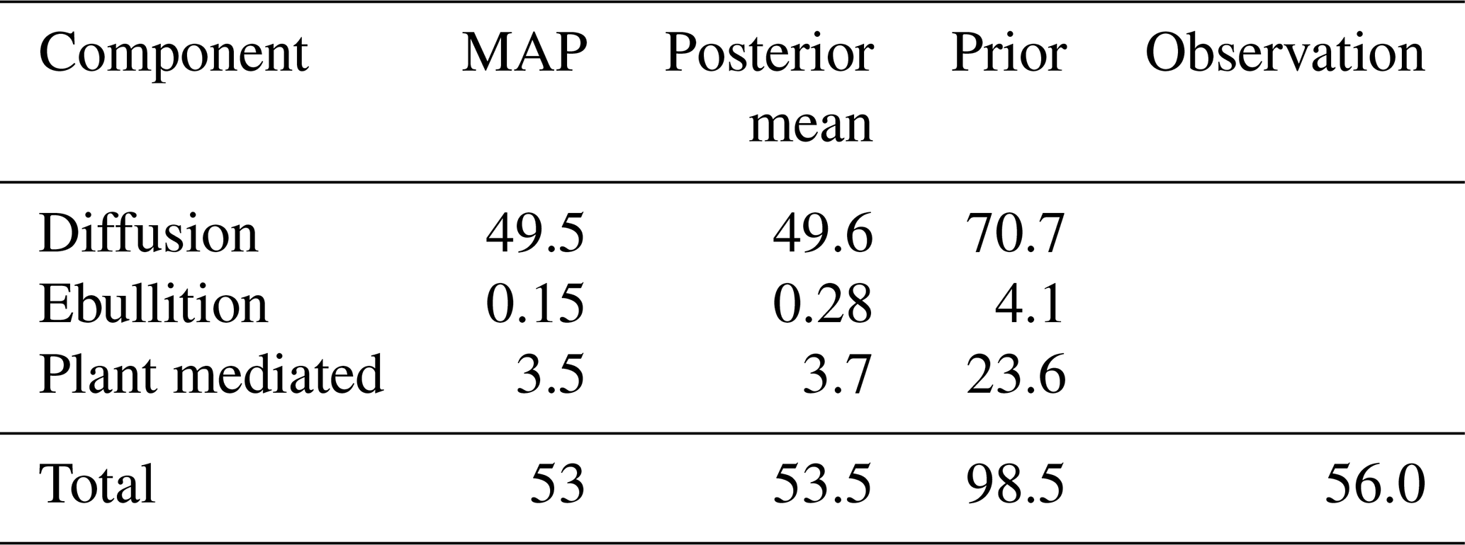
The largest reduction, however, was for ebullition (by around 92 %). This result is not surprising, as Wania et al. (2010), who provide the basic foundation of the CH₄ model in LPJ-GUESS, also reported almost virtually no ebullition to the surface at several sites. Figure 13 shows that no ebullition is estimated during the years 2008, 2010, and 2012. Here, it should be considered that the representation of ebullition in LPJ-GUESS is somewhat simplified using a curve-fitting equation to calculate the solubility and using the ideal gas law to convert the volume of CH₄ per volume of water into the corresponding number of moles. Due to this lack of detail and its fast timescale occurrence (mostly depends on the physical parameters such as temperature and pressure) and with no relevant parameters in the control vector, the optimisation could not alter the ebullition component directly. However, ebullition is indirectly controlled by parameters related to CH₄ production and transport when there is a high amount of saturated CH₄ available in the soil water. Thus, the optimisation can indirectly affect the ebullition. The total observed CH₄ flux from Siikaneva during the period of 2005 to 2014 was 56.0 gC m⁻², while the prior model estimate was 98.5 gC m⁻² (Table 6). After the optimisation, with the posterior mean estimate of parameter values, the model estimated a flux of 53.5 gC m⁻² with an estimated posterior uncertainty of ±4.82 gC m⁻². This shows a reduced model–data error after optimisation with a difference of only 2.5 gC m⁻².

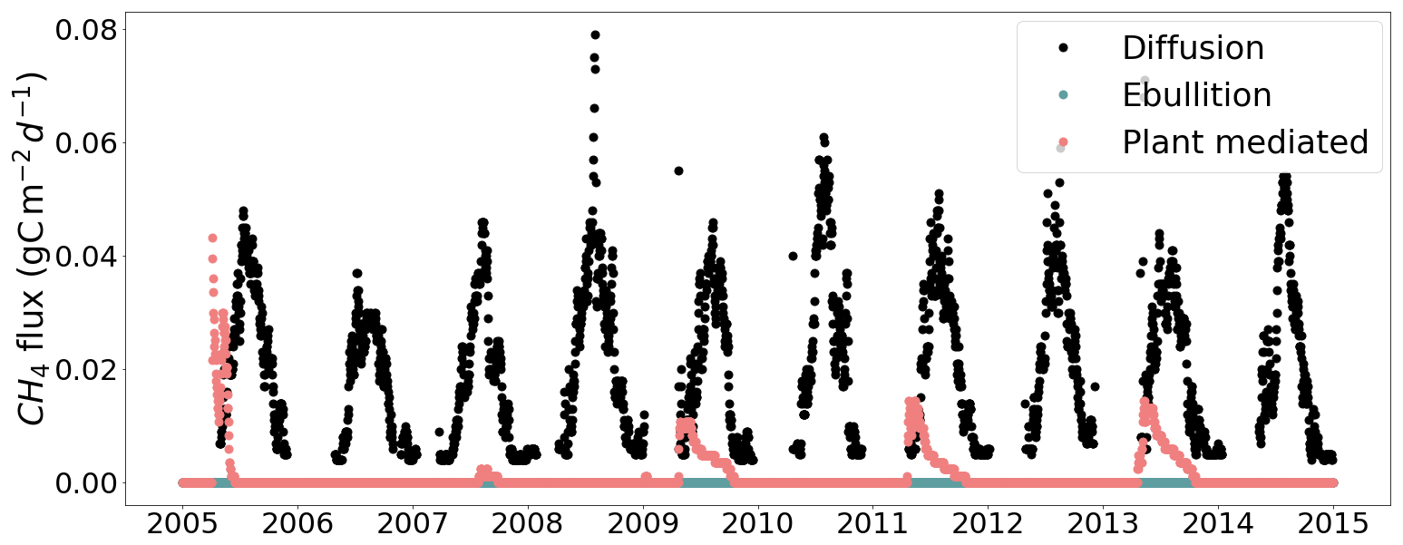
Figure 13 Time series for diffusion, ebullition, and plant transport using parameter values from the posterior mean estimate. A few outliers above 0.08 gC m⁻² on the vertical axis have been removed from the figure for better visualisation.

Table 6 Total emissions from flux components estimated from the MAP, posterior mean, and prior parameter values for all 10 years of the optimisation, given in grams of carbon per square metre.

4.2.3 Posterior process–process correlation

After the optimisation, the air fraction in the peat was increased, which is likely the cause of the enhanced diffusion. Diffusion is estimated in the model based on the soil porosity, water, temperature, and air fractions in the soil. Correlating the diffusion with the ebullition showed a negative result, i.e. illustrating the dominance of diffusion over ebullition (see Fig. 8b). A larger air fraction in the soil can also lead to an increase in plant-mediated emission, as the passive diffusion of air through the plant tissues depends on the amount of air in the soil/peat water (see Sect. 2.2.3). This can be seen in Fig. 8b as a comparatively high correlation between diffusion and plant-mediated transport. The increased tiller radius (r_tiller) in plants increases the A_tiller value (Eq. 8), thereby favouring faster diffusion through the aerenchyma cells. Ebullition is positively correlated with plant-mediated transport, indicating the occurrence of both of these components when there is a high concentration of CH₄ in the soil. This occurs when the water table is located close to the surface and when there is a higher density of graminoids. An increase in plant-mediated transport of gases to the soil increases the net pressure imposed by the gases in soil/peat water, which could also lead to increased ebullition.

4.3 Model error and fit to the observation

Except for ebullition, all of the prior process components exhibited larger variances in the annual errors compared with the posterior estimates (Fig. 11). The plant-mediated transport is the component with the largest error in the prior estimate. The posterior error estimates for this component showed nearly equal values, with a slightly higher value for the posterior mean estimate. A similar pattern can also be seen for diffusion. In contrast, the MAP error estimate for ebullition showed a higher value compared with the posterior mean error but interestingly also to the prior. The posterior mean error estimate for ebullition showed the lowest value.

The annual sums of flux components mentioned above are illustrated in Fig. 10a. It is clear from this figure that the prior process components had large inter-annual variance, especially for the first 3 years and the last year. A considerable reduction in variance is observed for both the MAP and posterior mean estimates. The reduction in the variance observed in posterior estimates is not proportional to the prior; however, the posterior estimates showed a comparatively high variance in the first and last years. In Fig. 10b, as described in Sect. 3.2.4, the posterior mean estimate shows a comparatively high variance (with respect to the MAP estimate) for the annual errors with a negative bias throughout the time period. In contrast, the MAP estimate showed a positive bias throughout the time period. Compared with the posterior mean estimate, the MAP estimate has considerably larger parameter values for ϕ_tiller and r_tiller; this could possibly be interpreted as slightly more CH₄ emission through the increased tillers of plants and, hence, the reason for the positive bias in the MAP estimate. Figure 11 also indicates a high percentage of annual plant-mediated emissions for the MAP estimate. The negative bias in the posterior mean estimate could be due to the additional wintertime emissions from the real-world wetlands, which are not captured in the model. In the model, the emissions start around early summer, once the soil is not frozen anymore. In addition, the large daily variability in the observations of the summertime fluxes is also not represented in the model. Overall, the posterior estimates of the annual fluxes are in good agreement with the observations, leading to a small model–data mismatch for both MAP and the posterior mean estimates.

4.4 Model inputs and uncertainty

As mentioned in Sect. 3.3, a somewhat pronounced systematic underestimation of emissions was observed in the years 2010, 2012, and 2013. None of the twin experiments exhibited these systematic errors, which indicates that the issue could be attributed to a structural model error (see Fig. 4). While the CH₄ module within LPJ-GUESS is relatively comprehensive when compared with many other similar models, the model's process description and parameterisation remain incomplete. For instance, in the real world, wind plays a crucial role in CH₄ emissions and its atmospheric concentration; however, wind speed is set to 0 for modelling convenience in LPJ-GUESS, thereby presenting a significant limitation. Similarly, the lack of the representation of air pressure, the simplified representation of ebullition (see Sect. 4.2.2), and the simplified representation of CH₄ production (see Eq. 2) are also a major limitations. Another reason for this mismatch could be the variations in the input climate data. The correlation plots of the input environmental variables of LPJ-GUESS and the CH₄ residuals (Fig. S3) indicate that, in these years, CH₄ emissions showed a comparatively high correlation with swr and air temperature, although precipitation did not show any significant relation. The results of the sensitivity study indicate that both the prior and posterior model estimates are significantly sensitive to the input variables. However, the posterior model estimate exhibited a considerable reduction in sensitivity, especially for swr and precipitation (see Sect. S5 and Fig. S5).

As mentioned in Wania et al. (2010), the flux components are determined by complex processes that depend on changes in many environmental factors. The model is unable to represent peak emissions caused by these microenvironmental changes. For instance, ebullition (one of the more complex CH₄ emissions processes in LPJ-GUESS, as explained in previous sections) depends on the volumetric content of wind and various gases as well as on hydrostatic and atmospheric pressure. However, the model does not use them as forcing variables. Ebullition is also affected by the concentration of CH₄ and the density of nucleation sites, which are difficult to represent in the model.

It should be noted that the incomplete state vector used for optimisation might have affected the optimised model result. The process representations in LPJ-GUESS are complex and interconnected, with a multitude of parameters directly or indirectly linked to CH₄ fluxes. Representing the indirect parameters can be intricate, as they may depend on other fluxes or model components. For instance, the soil module in LPJ-GUESS is intricately connected to the CENTURY model, featuring 10 soil compartments. Introducing a parameter related to soil temperature or the wtd into the framework would necessitate consideration of the intricacies of the CENTURY model. Furthermore, it might require the inclusion of additional flux species, such as net primary production (NPP), soil temperature profiles, or wtd. This would significantly increase the complexity of the problem, exceeding the scope of this paper. Given these caveats, the small negative biases obtained for the posterior mean estimates when compared against the observations (see Fig. 10b) are reasonable considering the quality and uncertainty in the input data used (see Sect. 2.1) and the complexity and structural issues of LPJ-GUESS.

4.5 Optimised simulation from LPJ-GUESS

A detailed time series distribution of prior and posterior model simulations plotted against the observations is shown in Fig. 12. The posterior model predictions were adjusted by the optimisation to fit the observations with considerable adjustment to the summer peaks. For example, the large peaks in the modelled emissions in 2005 and 2006, which largely contributed to the prior cost function, disappeared in the posterior emissions. In the following years, 2007 and 2008, the prior model simulations underestimated the observation, which also got corrected in the posterior. Furthermore, the posterior emissions largely capture the comparatively high peaks in the observations for the years 2010 and 2012, although the model still underestimated the observations. In 2013, the observations were high and the optimisation failed to capture this peak; rather, it tried to compensate for the underestimation by releasing a sudden high spike at the end of the summer that year. In winter months, the model simulated very low or almost zero fluxes (as discussed before), whereas, the observations showed a small emission (around 8.3 % of the assimilated total), often with some small spikes (possibly from the ebullition). This inability of the model to capture the wintertime emission has contributed to the posterior model uncertainty and model–data misfit.

A significant mismatch in soil temperature and wtd has been observed between the model and observations, especially during the wintertime (see Sect. S4 and Fig. S4). The model tends to overestimate wintertime temperatures and underestimate the wintertime wtd, indicating completely frozen soil with a very low wtd. This discrepancy could be a reason for the complete suspension of model CH₄ emissions during the winter. Observations show many days with a wtd above ground level, both in summer and winter. As the wtd is a key factor that can affect all flux components, this error could contribute to the misfits observed after the optimisation, although it cannot explain the systematic under estimation observed in the posterior. It should be noted that there are no considerable differences observed between the prior and posterior soil temperature or wtd.

As discussed in Sect. 4.2.3, the contribution of ebullition to the posterior estimate is comparatively negligible. Compared with the posterior, there were many emissions spikes observed in the prior estimate, especially during the beginning and the end of the summer months. Apart from these spikes, the prior CH₄ estimates during the summer were a bit low in most of the years. The posterior estimate has considerably reduced these high spikes and adjusted the summer peaks to match the observations better. On the other hand, while compromising for the summer peaks in the observations, the model with the optimised parameters often failed to capture the abrupt high fluxes in the daily observation and simulated them at slightly wrong times. The spike shown at the end of 2013 is an example of this mistiming. This is likely caused by errors in the meteorological input data and missing wind and pressure representations.

It can be seen from the Fig. 12 that the majority of the observations lie within the 95 % confidence interval of the posterior estimate. Often, the observation uncertainty overlaps the confidence interval, except for the summer peak times of 2010, 2012, and 2013 in which the observations showed strong peaks compared with the average values. The few outliers in the observations are not captured by the model; these could likely be measurement artefacts and/or due to environmental forcing not considered here, such as wind speed or air pressure.

4.6 Merits and shortcomings of the GRaB-AM framework

The advantages of the developed GRaB-AM framework include the ability of the MCMC method to escape local maxima or minima, making it more robust in this respect than gradient-descent-based methods. Furthermore, the MCMC method is derivative-free, thereby avoiding issues with computing gradients for very rough (non-continuous) functions. The adaptive part of the MCMC “learns” about parameter correlations and utilises these dependencies in the proposal, allowing it to better explore the parameter space. Potential issues for the MCMC are that very uneven cost functions can lead to the chain getting stuck (essentially, the local minima is too deep for the algorithm to escape). Here, we have alleviated this issue by tapering the cost function. We also acknowledge that the cost function could be improved, as the squared cost function essentially assumes Gaussian errors with equal variance for all values and ignores any temporal correlations. The observations are measured as time series, and concentration/flux observations are known to have spatio-temporal error correlations. Adapting the cost function to account for these factors would be of interest and is likely to have a larger impact on the posterior parameter uncertainties than on the estimates of the parameters.

In principle, the twin experiment should be able to recover all of the parameters completely. However, the twin experiment in this study did not completely recover the true values of some parameters, especially the ${\mathrm{CH}}_{\mathrm{4}}/{\mathrm{CO}}_{\mathrm{2}}$ parameter. This could be attributed to one or more of the following issues: (1) due to the complex and extremely non-linear nature of LPJ-GUESS, there is a high possibility of equifinality; (2) the high dimensionality of the problem and limited variability in the data could be a reason for the poor convergence of some parameters; and (3) the model is not fully constrained by the limited dimensions in both the data and the parameter space. Achieving complete convergence may require incorporating (a) additional complementary observations capable of constraining additional model processes and (b) additional parameters from different modules of the model that represent different model processes.

The failure observed in convergence is expected to yield suboptimal parameter estimates with overly optimistic posterior uncertainty estimates due to the equifinality problems in the real-data experiments. It may also result in slightly corrupted relationships between variables, leading to changes in the covariance structure of the posterior parameters estimated from the real data. Considering the high degree of non-linearity in the model, a single type of twin flux from a single site might not be sufficient to identify all of the parameters. Therefore, additional sites spanning a large climatic variability and/or different species of twin fluxes from the same site may be necessary. For instance, regarding the ${\mathrm{CH}}_{\mathrm{4}}/{\mathrm{CO}}_{\mathrm{2}}$ parameter, one reason for the poor recovery could be that the study only optimises the CH₄ component, leaving the CO₂ fluxes significantly off. Incorporating both CH₄ and CO₂ fluxes to address both sides of the ratio would lead to a more accurate convergence. However, a challenge in this approach would involve formulating cost functions for different observations in a manner that properly weights them to equally represent the information without diminishing their significance. These considerations are beyond the scope of this paper.

5 Conclusions

This study represents an initial effort to optimise the model process parameters controlling the simulation of wetland CH₄ fluxes within the LPJ-GUESS model using a Rao-Blackwellised adaptive MCMC technique based on Bayesian statistics. The assimilation framework has been shown to be able to retrieve true parameter values within the uncertainty limits discussed above by performing a set of twin experiments. Furthermore, we used eddy-covariance flux measurement data from a boreal wetland to calibrate the LPJ-GUESS model parameters for a site-specific simulation. The results demonstrate that the fit to the observation of the CH₄ simulation of a complex terrestrial DGVM like LPJ-GUESS can be systematically enhanced with a Bayesian parameter calibration. The results also show that the modelled processes and the estimated parameters were well constrained by the observations, leading to a substantial reduction in the posterior uncertainty in the simulated CH₄ emissions. However, we note here that, due to the equifinality problems identified in the identical twin experiments, the posterior parameter values contain compensating effects caused by the non-linearity of the model and the lack of an additional observational data constraint to uniquely identify each individual parameter. The results of the resampling experiment and the parameter and process correlations indicate that there are no redundant processes in the model description.

The robustness of the assimilation framework developed in this study calls for further application of the framework using observations from multiple sites in a simultaneous assimilation. Further validation of the framework's performance is necessary to confirm its applicability to other sites with diverse PFTs and climatic conditions. The relatively strong roughness in the shape of the cost function observed in this study is expected to be reduced in a multi-site assimilation experiment, as has been observed by Kuppel et al. (2012); this would provide additional observational data constraints to allow the retrieval of the global minimum of the cost function more easily and reduce the equifinality problem. These further applications are beyond the scope of this paper and will be investigated in future studies.