High-resolution downscaling of CMIP6 Earth system and global climate models using deep learning for Iberia

Deep learning (DL) methods have recently garnered attention from the climate change community for being an innovative approach to downscaling climate variables from Earth system and global climate models (ESGCMs) with horizontal resolutions still too coarse to represent regional- to local-scale phenomena. In the context of the Coupled Model Intercomparison Project phase 6 (CMIP6), ESGCM simulations were conducted for the Sixth Assessment Report (AR6) of the Intergovernmental Panel on Climate Change (IPCC) at resolutions ranging from 0.70 to 3.75^∘. Here, four convolutional neural network (CNN) architectures were evaluated for their ability to downscale, to a resolution of 0.1^∘, seven CMIP6 ESGCMs over the Iberian Peninsula – a known climate change hotspot, due to its increased vulnerability to projected future warming and drying conditions. The study is divided into three stages: (1) evaluating the performance of the four CNN architectures in predicting mean, minimum, and maximum temperatures, as well as daily precipitation, trained using ERA5 data and compared with the Iberia01 observational dataset; (2) downscaling the CMIP6 ESGCMs using the trained CNN architectures and further evaluating the ensemble against Iberia01; and (3) constructing a multi-model ensemble of CNN-based downscaled projections for temperature and precipitation over the Iberian Peninsula at 0.1^∘ resolution throughout the 21st century under four Shared Socioeconomic Pathway (SSP) scenarios. Upon validation and satisfactory performance evaluation, the DL downscaled projections demonstrate overall agreement with the CMIP6 ESGCM ensemble in magnitude for temperature projections and sign for the projected temperature and precipitation changes. Moreover, the advantages of using a high-resolution DL downscaled ensemble of ESGCM climate projections are evident, offering substantial added value in representing regional climate change over Iberia. Notably, a clear warming trend is observed in Iberia, consistent with previous studies in this area, with projected temperature increases ranging from 2 to 6 ^∘C, depending on the climate scenario. Regarding precipitation, robust projected decreases are observed in western and southwestern Iberia, particularly after 2040. These results may offer a new tool for providing regional climate change information for adaptation strategies based on CMIP6 ESGCMs prior to the next phase of the European branch of the Coordinated Regional Climate Downscaling Experiment (EURO-CORDEX) experiments.

1 Introduction

The Sixth Assessment Report (AR6) of the Intergovernmental Panel on Climate Change (IPCC) was released in August 2021, dramatically calling for urgent action to reduce global greenhouse gas emissions (GGEs) due to the scale of the projected changes for the climate system from the mean state to extremes (IPCC, 2021). The results in the report are based on the Coupled Model Intercomparison Project phase 6 (CMIP6) simulations, which were performed using Earth system and global climate models (ESGCMs), and included runs with a spatial resolution in the range of 0.70 to 3.75^∘. The IPCC report projects worrying changes in global-scale extreme events, such as significant increases in the frequency and intensity of heat waves, droughts, and extreme precipitation. Although based on global simulations, the AR6 showed particularly pronounced changes on a regional level in some climate change hotspots, like the Mediterranean region (Turco et al., 2015; Cos et al., 2022; Lionello and Scarascia, 2018).

It is widely accepted that most resolutions used by ESGCMs are still too coarse to represent many regional- to local-scale processes that define the local climate (Randall et al., 2007; Soares et al., 2012; Rummukainen, 2016). This disadvantage highlights the necessity for downscaling methods, at a higher resolution, which often provide regional to local fine-scale information, which is crucial for impact and adaptation studies. There is a plethora of downscaling methods, including dynamical ones using regional climate models (RCMs), statistical ones using statistical downscaling methods (SDMs), and, recently, an umbrella group of the latter, designated as artificial intelligence (AI) approaches, which include machine-learning (ML) and deep-learning (DL) methods.

RCMs are forced at the boundaries by ESGCMs (Dickinson et al., 1989; Giorgi and Bates, 1989; Giorgi and Mearns, 1991; McGregor, 1997; Christensen et al., 2007), using higher resolutions (∼ 10 km) in limited area domains, which significantly improve the description of regional to local climates (Giorgi and Mearns, 1999; Laprise, 2008; Rummukainen, 2010, 2016; Feser et al., 2011; Soares et al., 2012, 2017a, b; Rios-Entenza et al., 2014; Giorgi et al., 2016; Lucas-Picher et al., 2017; Cardoso et al., 2019). Nevertheless, considering local and, especially, sub-daily climate features, RCMs still present limitations in capturing sub-grid processes such as convection (Prein et al., 2013). In order to bridge this gap, RCMs are running at very high resolutions, usually described as convective-permitting resolutions (approximately 1 km), where deep convection is explicitly resolved by the grid mesh at grid spacing below 3 km (Prein et al., 2015; Coppola et al., 2020; Pichelli et al., 2021; Soares et al., 2022).

SDMs are based on the establishment of empirical relationships between large-scale atmospheric predictors and local observed predictands describing local climate (Wilby and Wigley, 1997; Fowler et al., 2007; Nikulin et al., 2018; Hertig et al., 2019; Maraun et al., 2019; Gutiérrez et al., 2019a; Rössler et al., 2019; Soares et al., 2019; Widmann et al., 2019). Subsequently, projections of future regional to local climate variables are determined from future large-scale atmospheric conditions. SDMs include model output statistics and perfect-prognosis approaches (Maraun et al., 2010, 2017). However, when compared to dynamical downscaling, the model formulation of SDMs lacks physical constraints and, in general, does not ensure a full multivariate consistency (Le Roux et al., 2018). Since SDMs use observations for training, they are able to overcome the systematic biases often displayed by RCMs. Additionally, since SDMs are not computationally demanding, the need for large computational infrastructures is avoided.

There is a continuous improvement in SDMs, and new AI approaches are being proposed for climate applications, with deep learning (DL) being one of the most promising. DL is a subdomain of machine learning (ML). In ML, the models learn the optimal value of their parameters automatically. Since parameter tuning is based on the input data fed to the model, the model is able to make predictions when forced by new data (see Alzubi et al., 2018, for an overview of ML). Unlike “shallow” learning models (e.g., random forests and support vector machines), DL models learn non-linear relationships between data due to their “deep” layered structure. DL has become a common approach in research over the past decade (Schmidhuber, 2015), including in Earth sciences in the last few years (Reichstein et al., 2019), thanks to advances in computational power and data availability. For example, the European Centre for Medium-Range Forecasts (ECMWF) features DL as the main showcase in its Destination Earth project (Bauer et al., 2021), which will attempt to create digital twins of the Earth system in the next decade.

The most common DL model type is the artificial neural network (ANN), an attempt to design an artificial analog to the biological neural networks that exist in the human brain. One of the most used types of ANNs is convolutional neural networks (CNNs). These models are widely used in the field of computer vision, as they extract information and identify objects in images (LeCun and Bengio, 1995). However, the value of CNNs is not restricted to computer vision, as CNNs have been used in other research areas, including in Earth sciences, for example, in model parameterization (Chantry et al., 2021a) and ensemble postprocessing (Rasp and Lerch, 2018), showing promising results. Climate downscaling is another promising area benefitting from the implementation of CNNs. Early attempts at downscaling using simple ANN structures were not compelling due to limited input data, computational resources, and scarcer observations (e.g., Wilby et al., 1998; Trigo and Palutikof, 1999). Recent studies have shown more favorable results, equalling and even surpassing classic SDMs (e.g., Baño-Medina et al., 2020; Hernanz et al., 2022; Baño-Medina et al., 2022). Recently, and for the first time, Baño-Medina et al. (2022) were able to downscale climate projections with the aid of DL for precipitation and temperature, based on a set of global climate models (GCMs) from the Coupled Model Intercomparison Project phase 5 (CMIP5). These authors showed that DL reduced the biases in the historical period when compared to an ensemble of RCMs with 0.44^∘ resolution from EURO-CORDEX (European branch of the Coordinated Regional Climate Downscaling Experiment). In addition, the resulting climate change signals have similar spatial patterns to those obtained from the RCMs, and when looking at the uncertainty, the DL preserves the uncertainty of the climate change signal for temperature and reduces it for precipitation.

Despite their promising results, DL methods are viewed with caution in the scientific community due to their black-box nature. DL models usually have thousands (if not millions) of trainable parameters that hinder a physically based explanation for the quality of their results. There have been attempts to improve the understanding of models' reasoning (e.g., Carter et al., 2018), building an overall framework for DL studies in Earth sciences, including weather/climate modeling and postprocessing, and generating consistent intercomparable studies (Reichstein et al., 2019; Chantry et al., 2021b; Haupt et al., 2021). As a result, the first benchmark dataset for data-driven weather forecasting has been created (Rasp et al., 2020). DL presents other general limitations, including the need for hardware (graphics processing units or GPUs accelerate the model training, while the more common central processing units or CPUs can be computationally costly; Chantry et al., 2021a). Other DL limitations concern the climate research field. Lack of explicit physics in the DL models and the need to split the data in a way that includes long-term patterns and trends (e.g., El Niño–Southern Oscillation or ENSO and global warming) in both training and test phases for long-term datasets (Schultz et al., 2021) are examples of said limitations.

The Iberian Peninsula, within the Mediterranean basin, is a known climate change “hotspot” (Planton et al., 2012; Diffenbaugh and Giorgi, 2012; Turco et al., 2015; Russo et al., 2019; Cos et al., 2022) due to its high vulnerability to warming and drying conditions (Argüeso et al., 2012; Cardoso et al., 2019; Soares et al., 2017a, b; Lima et al., 2023a, b; Soares and Lima, 2022), leading to high occurrence of extreme events, such as droughts, heat waves, and wildfires (Hoerling et al., 2012; Bento et al., 2022, 2023; Soares et al., 2023a). Future projections point to a warming trend that is stronger for daytime values during summer and autumn than in other seasons, resulting in an amplification of the daily and annual temperatures (Cardoso et al., 2019; Lima et al., 2023a). Also, a significant reduction in the mean precipitation is projected throughout the entire year (Argüeso et al., 2012; Lima et al., 2023a; Soares et al., 2017a). Concomitant with the projected warming and drying trends, the occurrence of hot and dry extreme events is expected to become more frequent, intense, and longer (Hoerling et al., 2012; Lima et al., 2023b), which may have significant impacts on human and natural sectors, such as agriculture (Bento et al., 2021), forests (Palma et al., 2015, 2018), coastal areas (Pereira and Coelho, 2013), and water resources (Soares and Lima, 2022). The Iberia01 regular gridded product (hereafter Iberia01) is the highest-resolution observational daily dataset including mean, maximum, and minimum temperatures and precipitation, covering the full domain of continental Iberia (Herrera et al., 2019). Iberia01 is commonly used for assessing the performance of ESGCMs (Soares et al., 2022), RCM results (Herrera et al., 2020; Careto et al., 2022a, b), building of multi-model ensembles for climate change assessments (Soares et al., 2023a; Lima et al., 2023a, b), and other studies, such as those related to water availability (Soares and Lima, 2022) and droughts (Páscoa et al., 2021; Soares et al., 2023a).

The most consistent and widely used high-resolution climate change dataset for Iberia remains the EURO-CORDEX and CORDEX-Core runs (Jacob et al., 2014, 2020). These regional climate simulations were forced by the previous CMIP5 global climate simulations and are becoming less useful after the recent release of the CMIP6 results forced by the Shared Socioeconomic Pathway (SSP) and Representative Concentration Pathway (RCP) greenhouse gas emissions scenarios. At present, the new EURO-CORDEX simulations protocol, forced by CMIP6 runs, is being finished, and widespread availability of new simulations and results for the scientific community and society is not expected before 1–2 years' time. Additionally, the building of new multi-model and multi-approach ensembles is highly beneficial to assess the robustness and uncertainty of future climate projections (Lima et al., 2023a). The increasing need for exploring and updating regional climate information for Iberia requires and benefits from the use of other approaches to downscale the current CMIP6 runs.

In the present study, a DL methodology based on the work of Baño-Medina et al. (2022) is used to downscale, in a consistent manner, the CMIP6 runs at high resolution for Iberia. A matrix of plausible futures is used to select the CMIP6 models considered to be in agreement with the EURO-CORDEX evaluation study (Sobolowski et al., 2023). The DL algorithm is trained using ERA5 and compared to the high-resolution regular gridded dataset Iberia01 (Herrera et al., 2019) for the current climate, covering the period 1979–2014, and is then used to downscale future projections in agreement with four SSP–RCP scenarios, namely SSP1–RCP2.6, SSP2–RCP4.5, SSP3–RCP7.0, and SSP5–RCP8.5 (O'Neill et al., 2016), for three future periods throughout the 21st century, namely the beginning of the century (2015–2040), middle of the century (2041–2070), and end of the century (2071–2100). First, different architectures of DL are trained and evaluated for the present climate and then multi-model projections are performed, based on a simple-averaged multi-model ensemble approach. This study is focused on four of the main climate variables and their extremes: minimum, mean, and maximum temperatures and precipitation. The main goals of this study are to understand the accuracy of downscaling CMIP6 GCMs to a much finer spatial resolution using DL and to take advantage of the advancing AI methods to compile information that may be crucial to timely assist mitigation and adaptation plans being developed at the national, regional, and local levels within Iberia.

2 Data and methods

2.1 Study area

The Iberian Peninsula (IP) is located in the southwestern tip of Europe (Fig. 1), bordered by the Atlantic Ocean and the Mediterranean Sea. The IP sits in a climate transition zone between the arid and semiarid climates of subtropical regions and the humid temperate climates of northern Europe. Despite having a surface area of smaller than 600 000 km², it shows a diverse climate, with significant regional variations. In fact, while the northern and northwestern regions are marked by long rainy seasons and temperate summers, the south and southeast are characterized by long and hot summers and a clear dry season. The interior regions are defined by a continental climate, with hot summers and cold winters. Additionally, local and regional topographic features play a significant role in modulating climate features throughout the IP. Here, the IP domain is considered to be the land area between 36 and 44^∘ N and ^∘ W and 4^∘ E (Fig. 1; inside the orange line). The predictor domain (Fig. 1; dashed red line) is a larger region than the IP domain to ensure that large-scale phenomena are included in the information provided by the predictors to train the DL models.

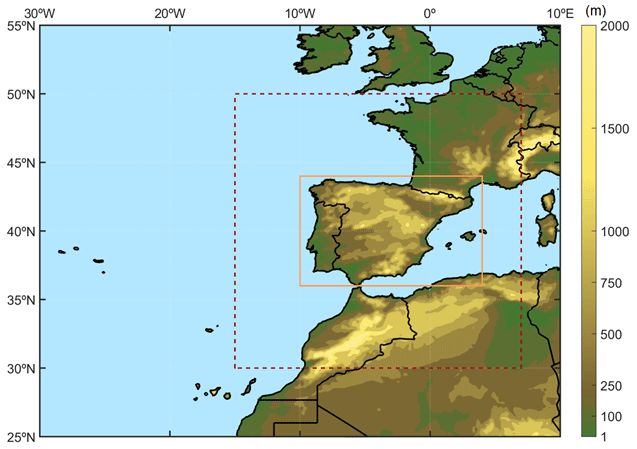
Figure 1 Consideration of western Europe and northwestern Africa topography (m) and of the domains of the Earth system and global climate model predictors (dashed red line) and predictands (full orange line).

2.2 ERA5 reanalysis

ERA5 is the latest European Centre for Medium-Range Weather Forecasts (ECMWF) reanalysis (Hersbach et al., 2020) produced within the Copernicus Climate Change Service (C3S). ERA5 provides a comprehensive, high-resolution record of the global atmosphere, land surface, and ocean from 1950 onwards. Benefitting from advanced research and model physics development, outputs are archived at 0.25^∘ × 0.25^∘ horizontal and 1 h time resolutions, considering 137 atmospheric levels up to 0.01 hPa. The ECMWF Integrated Forecasting System (IFS) Cy41r2, used operationally for forecasting from March to November 2016, is used to produce ERA5. Additional details are available in Hersbach et al. (2020). Here, the period from 1 January 1979 to 31 December 2014 is considered. The original ERA5 reanalysis data were interpolated to a 1^∘ × 1^∘ horizontal resolution, using a bilinear interpolation method, to build a common grid to the CMIP6 ESGCMs (Sect. 2.3).

2.3 CMIP6 Earth system global climate models

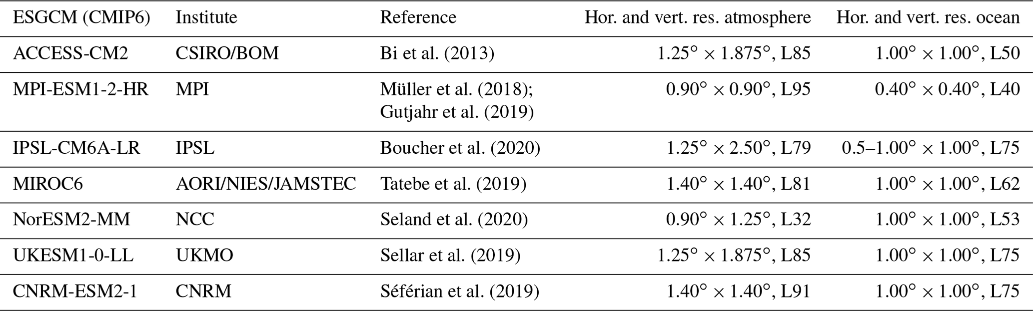
The ESGCMs selected for the current study closely follow the model array built in Sobolowski et al. (2023) for the ongoing CMIP6 dynamical downscaling that is being performed (i.e., the regional climate model simulations of EURO-CORDEX phase II). The authors thoroughly analyzed the ability of the CMIP6 ESGCMs to describe the most important large-scale features that define the European climate, such as the storm track position, and that span the AR6 IPCC climate sensitivity range. The ESGCMs considered are listed in Table 1; understandably, the list is additionally constrained by the availability of the predictors data. The predictor data were extracted for the domain in Fig. 1 (inside the dashed red line), limited by 30^∘ N–50^∘ N, 15^∘ W–7^∘ E, and then interpolated to a common grid at a 1^∘ × 1^∘ resolution, using the bilinear interpolation method.

2.4 Iberia01 observational regular gridded dataset

The Iberia01 regular gridded product is the highest-resolution observational daily dataset including mean, maximum, and minimum temperatures and precipitation that covers the full domain of continental Iberia (Herrera et al., 2019). This observational dataset was built using an unprecedented number of ground station observations, 275 for temperatures and 3486 for daily accumulated precipitation, resulting in a high-quality regular gridded dataset at 0.1^∘ × 0.1^∘ horizontal resolution. Here, the Iberia01 product is used both to calibrate and evaluate the deep learning approach for the period 1979–2014 (same as ERA5).

Table 1 CMIP6 Earth system global climate models. Note that “Hor. and vert. res.” stands for horizontal and vertical resolution.

2.5 Deep learning methodology

Convolutional neural networks (CNNs) are deep learning (DL) model structures specializing in extracting features automatically from geospatial data. The architecture of a CNN model includes convolutional layers that perform feature identification and extraction using filters that apply the mathematical operation of cross-correlation to the data (LeCun and Bengio, 1995; see Fig. 3 of Baño-Medina et al., 2020). The general outline of one epoch, i.e., a full cycle of the training phase, is as follows:

• The 2D filters in a convolutional layer “scan” the set of predictor variables, computing a set of filter maps based on each filter, highlighting different features/patterns of the original data. These filter maps are then used as input for the following convolution layer.

• The output of the final convolutional layer is flattened (reshaped to 1D) before being fed to the fully connected (dense) layer that follows.

• The units in a dense layer are connected to every unit in the previous and following layers, allowing the network to learn potential relationships between all units in successive layers. The final dense layer must have the size of the target data in order to generate the predictions.

• The predictions are compared with the observations by calculating the loss, according to the loss function defined by the user.

• Finally, the model attempts to lower the loss by the use of the stochastic gradient descent optimization algorithm, tuning the parameters of each model layer according to the direction of the gradient that minimizes the loss the fastest. This process begins in the output layer, computing the gradients on that layer, and backtracks all the way to the first convolutional layer in what is known as the back-propagation algorithm.

The model then repeats the training until it reaches a convergence mark defined by the user (usually a set number of epochs after the loss stops decreasing). While the learnable parameters are optimized automatically by the model, there is a set of hyperparameters that is defined by the user, including the following:

• the maximum number of epochs that the model can run;

• the batch size of observations used to tune the model in each training cycle; and

• the learning rate at which the model incorporates new information after each epoch.

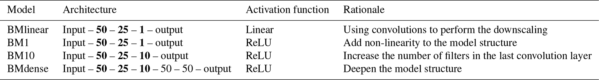
The main goal of DL is to achieve generalization; i.e., the ability to make quality predictions when given new, never-before-seen data (extrapolation). Such a feature is particularly important when training DL models for climate studies, due to global warming and other long-term trends. The model structures considered in this study were retrieved from the Baño-Medina et al. (2020) and are described in Table 2. Although all models have similar structures, differing only in the small details, they are designed in such a way that every model is slightly more complex than the previous one. All models comprise the following:

• three convolutional layers (the first two layers have 50 and 25 filters each);

• a final dense layer that outputs the predictions; and

• the same hyperparameters (batch size = 100 and learning rate = 0.0001).

The differences among the models are as follows:

• The third convolutional layer has 1 filter in BMlinear and BM1 architectures and 10 filters in BM10 and BMdense architectures.

• BMdense presents two additional dense layers, both with 50 units, prior to the output layer.

• The activation function in every layer of every model is the rectified linear unit (ReLU), a non-linear function, except in BMlinear, in which the function is linear.

The loss function used for the temperature predictions is based on the mean squared error. For precipitation, however, the DL models feature a multi-output structure (see Fig. 3 in Baño-Medina et al., 2020). Instead of predicting precipitation directly, the model attempts to obtain three parameters: the shape (alpha) and scale (beta) of the gamma distribution and the probability of precipitation (p). This is achieved by applying a custom loss function that computes the negative log likelihood of the Bernoulli–gamma distribution (Cannon, 2008), following the methodology presented in Baño-Medina et al. (2020). The precipitation value is obtained by multiplying the alpha and beta parameters.

Table 2 CNN architectures used in this study (adapted from Baño-Medina et al., 2022). The architecture is divided into one input and one output layer and several hidden layers in between. Numbers represent the units in each hidden layer, with convolutional layers in bold; otherwise, dense layers are given. The input format is lat × long × 15 (five predictors times three pressure levels), and the output is a 6523 × 1 vector (the number of 0.1^∘ land grid points over Iberia).

2.6 Selection of predictors, training, and evaluating

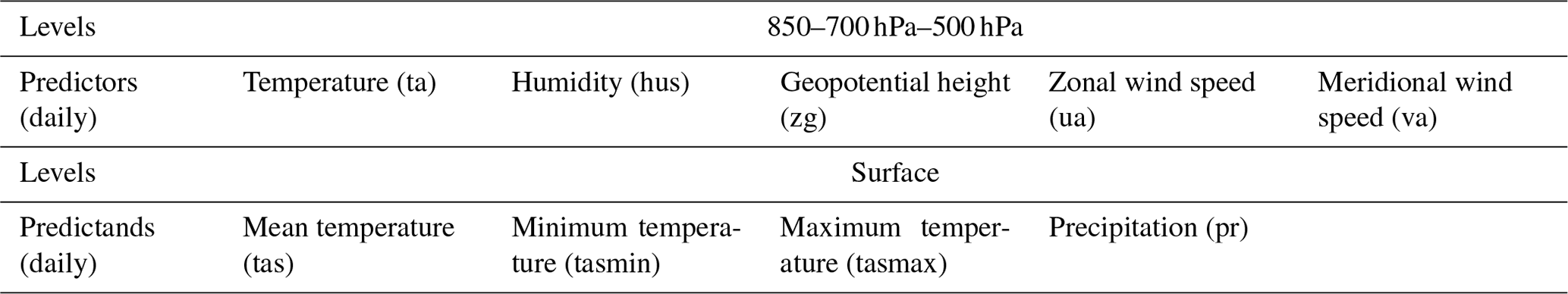
The predictors selected follow the Baño-Medina et al. (2022) study and are included in Table 3. The data were pre-processed before being used to train and evaluate the DL models. The ERA5 variables, used as predictors, were standardized to facilitate the training of the DL models. Grid points with missing data in the CMIP6 ESGCMs were filled with an average of the surrounding grid points. If the surrounding grid points had missing data as well, then a domain average was applied. Afterwards, the dataset was standardized (with the same parameters used for ERA5). The ESGCMs were bias-corrected in relation to ERA5 through a simple mean-variance scaling method. The climate change trend was removed in the future scenarios before the bias correction and reintroduced afterwards (Vrac and Ayar, 2017).

Two stages were pursued with the aim of training and evaluating the four architectures (Fig. 2). The first stage was to train them using ERA5 predictors (Table 3), considering the 1979–2004 period, validating their performance between 2005 and 2009, and finally testing the architectures for the period 2010–2014. This process was performed to obtain each of the four predictands, namely daily mean temperature (T), daily minimum temperature (T_min), daily maximum temperature (T_max), and daily accumulated precipitation (Pr) (Table 3). The results of the DL downscaled predictands from ERA5 were then compared with the Iberia01 reference data. In this case, since the DL used ERA5 reanalysis predictors, the evaluation was performed with daily synchronized climate data. This evaluation, conducted between 2010 and 2014, was based on error metrics such as the bias, the root mean squared error (RMSE), the standard deviation ratio (SDR), the Perkins' skill score (PSS), and the relative operating characteristic skill score (ROCSS).

The mean bias, used for temperature and precipitation is defined as

$$\begin{array}{}\text{(1)}& \mathrm{Bias}={\displaystyle \frac{\mathrm{1}}{N}}{\sum }_{k=\mathrm{1}}^N\left(m_k-o_k\right),\end{array}$$

where o_k and m_k are, respectively, the observed and modeled time series, and N is the total number of grid points.

The root mean squared error (RMSE), used for temperature and precipitation, is defined as

$$\begin{array}{}\text{(2)}& \mathrm{RMSE}=\sqrt{{\displaystyle \frac{\mathrm{1}}{N}}{\sum }_{k=\mathrm{1}}^N{\left(m_k-o_k\right)}^{\mathrm{2}}}.\end{array}$$

The standard deviation ratio, used only for temperature, is expressed as

$$\begin{array}{}\text{(3)}& {\mathit{\sigma }}_n={\displaystyle \frac{{\mathit{\sigma }}_{\mathrm{m}}}{{\mathit{\sigma }}_{\mathrm{o}}}}={\displaystyle \frac{\sqrt{\frac{\mathrm{1}}{N}{\sum }_{k=\mathrm{1}}^N{\left(m_k-\underset{\mathrm{¯}}{m}\right)}^{\mathrm{2}}}}{\sqrt{\frac{\mathrm{1}}{N}{\sum }_{k=\mathrm{1}}^N{\left(o_k-\underset{\mathrm{¯}}{o}\right)}^{\mathrm{2}}}}},\end{array}$$

where σ_o and σ_m are standard deviations of the observed and modeled time series, respectively, while $\underset{\mathrm{¯}}{o}$ and $\underset{\mathrm{¯}}{m}$ represent the respective mean values.

The Perkins' skill score (PSS; Perkins et al., 2007) quantifies the model's ability to reproduce the observed probability distribution functions (PDFs) as follows:

$$\begin{array}{}\text{(4)}& S=\mathrm{100}\times {\sum }_{i=\mathrm{1}}^{B}min\left[E_{\mathrm{m},i},E_{\mathrm{o},i}\right],\end{array}$$

where E_m and E_o are, respectively, the modeled and observed empirical PDFs, and $min\left[E_{\mathrm{m},i}{E}_{\mathrm{o},i}\right]$ is the minimum between the two values. B is the total number of bins used to compute the PDF.

Finally, the relative operating characteristic skill score (ROCSS) is given by

$$\begin{array}{}\text{(5)}& \mathrm{ROCSS}=\mathrm{2}\times \text{Area under the ROC curve}-\mathrm{1}.\end{array}$$

For the extreme values, the 2nd and 98th percentiles of T, the 10th (90th) percentile of T_min (T_max), and the 98th percentile of Pr were computed and compared with those from Iberia01 (bias).

The second stage consisted in training the DL architectures with ERA5; this time, the complete 1979–2014 period was used. These architectures were then used to downscale the individual CMIP6 ESGCMs for the same period for each of the four predictands. The resulting DL downscaled ESGCMs, at 0.1^∘ horizontal resolution (ESGCM-DL), are non-synchronized with the Iberia01, and consequently, only a statistical comparison was performed. Therefore, Julian years with 365 multi-year daily means were computed for each ESGCM-DL and for the Iberia01, and a performance evaluation based on the same error metrics as in the first stage was conducted. Finally, a simple average ensemble was built for each architecture, containing seven ESGCM-DL models, and compared to the 1^∘ ESGCM ensemble, the 1^∘ ERA5 reanalysis, and the interpolated 0.1^∘ ERA5 reanalysis.

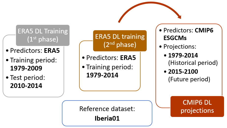
Figure 2 Summary of the two phases of the methodology (detailed in Sect. 2.6) describing the predictors and training and projections periods considered in each phase.

Table 3 ERA5 and CMIP6 predictors and predictands and the respective atmospheric levels.

2.7 Future climate projections

The present climate historical period considered here corresponds to 1981–2010. The future climate projections are focused on three periods: 2015–2040 (beginning of the 21st century), 2041–2070 (middle of the 21st century), and 2071–2100 (end of the 21st century), encompassing four CMIP6 SSPs (Rozenberg et al., 2014; O'Neill et al., 2016), namely SSP1–2.6, SSP2–4.5, SSP3–7.0, and SSP5–8.5. These scenarios range from a strong mitigation level, resulting in low greenhouse gas emissions (GGEs), with CO₂ emissions cut to net zero around 2075 (SSP1–2.6); an intermediate trajectory of future GGEs, with CO₂ emissions maintaining current levels until 2050 and then reducing, but not achieving, net zero by 2100 (SSP2–4.5); and, finally, two scenarios with increasing GGEs with SSP3–7.0 and SSP5–8.5, where the former considers that CO₂ emissions double by 2100, and the latter considers a 3-fold increase by 2075. In this study, results of future climate projections correspond to anomalies (differences) between the future and the historical climatological values, as given by a simple averaged multi-model ensemble consisting of all ESGCM-DL outputs. It should be noted that the projected temperature increase depends on the chosen historical period. Downscaling using the four DL algorithms is performed for each ESGCM considered in this study (Table 1) for the disclosed future periods. As reference, the change signal linked to all ESGCMs is also computed. The future ESGCM-DL-projected climate of Iberia is analyzed in terms of mean climate and extreme values. Anomaly maps for the annual projected changes for Iberia are presented for all variables, where the differences between the 1^∘ ESGCMs and 0.1^∘ ESGCM-DL projections are highlighted. Box plots summarizing the projected changes (median, interquartile range, and variability) are also presented for the four predictands.

3 Results

3.1 Evaluation of DL forced by ERA5

The four DL architectures are trained and validated with ERA5 for the 1979–2004 and 2005–2009 periods, respectively, and finally tested during 2010–2014 against Iberia01 considering minimum, mean, and maximum temperatures and precipitation. The performance evaluation metrics are shown in Fig. 3 (T), Fig. 4 (T_min), Fig. 5 (T_max), and Fig. 6 (Pr). The comparison between the ERA5 (interpolated to 0.1^∘ horizontal resolution; iERA5 from here on) and Iberia01 is also shown as a reference for all fields (dark gray box plot).

Considering T (Fig. 3), the following three main outcomes emerge: (1) all of the DL approaches display rather small errors and even slight improvements in comparison with iERA5, such as concerning RMSE and the PSS; (2) the DL architectures present less variability in accuracy metrics (bias) than iERA5, but in some cases, the error distribution of the latter is more closely centered around zero than for the DL outcomes; and (3) the four architectures present small biases for extreme values. When considering the total bias, the four architectures show somewhat interchangeable results, with median values slightly below zero for BMlinear, virtually zero for BM1, and slightly over zero for BM10 and BMdense. The small warm bias found for the 2nd percentile of T is observed both in the DL outcomes and in the iERA5. However, the cold bias found in the 98th percentile of T is only found in the DL outcomes, with values close to zero for the iERA5. Regarding the RMSEs, DL results show lower variability ranges than iERA5 and overall lower median values with increasing DL complexity. The interquartile range for the RMSEs of the DL results encompasses values from 1.25 to 1.5 ^∘C. In terms of SDR, in relation to Iberia01, the iERA5 shows the median value closest to 1; however, it also shows the largest interquartile distance and largest variability range (from ∼ 0.90 to ∼ 1.08 when compared with ∼ 0.93 to ∼ 1.04 for the DL outcomes). Finally, regarding the PSS, the four architectures show more similarity between distributions of T with Iberia01 than the iERA5. A distinction between the DL outcomes for this error metric is rather unnoticeable.

Regarding T_min (Fig. 4), the overall results show the following: (1) the DL architectures present better results in comparison to Iberia01 than the simple interpolation of ERA5, showing lower RMSEs, biases closer to zero, and larger PSS values; and (2) the four architectures show, to some extent, similar results between them. Following a more detailed analysis, the median biases presented by the four architectures are all near-zero, while the iERA5 shows a median bias larger than 1 ^∘C. Furthermore, when comparing the bias of the architectures to the interpolated ERA5, a lower interquartile range (circa 1 ^∘C) is observable in the first range compared to the latter (∼ 2 ^∘C). Additionally, a narrower extreme bias variability range (about 2.5 ^∘C versus about 4 ^∘C, respectively) is seen. Results for extreme low temperatures (bias p10) are in line with the total bias; nevertheless, these results show a slight tendency to lower median biases as the complexity of the architecture increases. This is also noticeable in the precision metric, with reduced RMSEs for increasing DL architecture complexity. However, here, BM10 and BMdense show very similar results. All architectures present median RMSEs below 2 ^∘C, which is the third quartile of the three more complex ones below this value as well. The maximum RMSE does not surpass 3 ^∘C. On the other hand, the iERA5 shows a median RMSE slightly above 2 ^∘C, the third quartile close to 3 ^∘C, and a maximum value above 4.5 ^∘C. Similar to the T results in Fig. 3, the median SDR is closer to 1 for the iERA5; nevertheless, the DL architectures show greater variability ranges for T_min in comparison to T. Among the architectures, BMdense is the one with a standard deviation ratio median closer to 1. Finally, considering the PSS values, it is once again noticeable that the distributions of the downscaled ERA5 using DL and Iberia01 tend to match better with the increase in complexity of the architectures.

When assessing T_max (Fig. 5), the following three main results may be highlighted: (1) all the error metrics are improved by the DL methods when compared with iERA5; (2) the DL architectures show much less variability in the biases and RMSEs in comparison to iERA5 (having Iberia01 as reference); and (3) the four architectures show, to some extent, similar results between them. In terms of bias, and considering the four architectures, neither T_max nor the extreme T_max show cold or warm biases, as both are centered around zero. Conversely, iERA5 shows a cold bias in both cases. Once again, the precision tends to be larger with more complex DL architectures, with BMdense showing lower RMSEs. The T_max SDR between BM10 and Iberia01 seems to indicate a better agreement than BMlinear, BM1, and BMdense. Nevertheless, the four architectures present SDR values closer to 1 when compared with iERA5. Finally, the matching between the four DL architectures outcomes distributions and Iberia01 is greater than for iERA5. The high-quality DL results for temperatures with regard to iERA5 are rather promising, since those variables are assimilated by ERA5.

For Pr, the error metrics from the comparison between the DL downscaled ERA5, iERA5, and Iberia01 are shown in Fig. 6. In this case, between the four architectures, BMdense is the most accurate and precise one, also surpassing iERA5. While the iERA5 shows an overall slightly negative bias (median of −8 mm), the DL outcomes show generally positive values (between 1 and 10 mm). Considering the extreme Pr (98th percentile), all approaches show an underestimation, performing slightly worse than the iERA5, despite the lower error variability ranges. The distributions of the RMSEs of iERA5 and BMlinear, BM1, and BM10 show somewhat similar results for the median and overall variability. In this case, BMdense presents the best results. Finally, the ROCSS shows that all four DL architectures have better skill at representing Pr over the Iberian Peninsula, in comparison with iERA5, with median values ranging between 0.82 and 0.86, which contrasts with 0.67 for iERA5.

The results from Figs. 3 to 6 show that the four DL architectures are successful in downscaling temperature and precipitation from ERA5 at high resolution, presenting, in the vast majority of instances, a better performance than iERA5. Given the similar behavior of the four architectures, choosing the “best” one is not straightforward. BM10 and BMdense show the best precision (RMSEs) for the four variables (with BMdense being the most precise). However, considering the biases, BMdense produces the best results for 10th percentile T_min, BMlinear comes first for the 2nd percentile of T, and BM10 produces more accurate results for T_max. Regarding Pr, BMdense and BM1 retain the best performance for the mean and 98th percentile. Therefore, a clear distinction between architectures for all variables is not meaningful. Therefore, and assuming that all DL architectures are able to partially contribute to the overall performance of the downscaled datasets, the ensemble-building process considers all DL downscaling equally for each ESGCM.

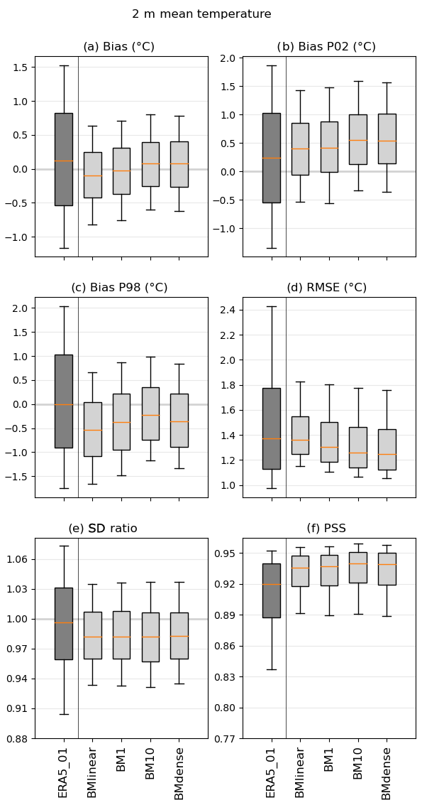
Figure 3 Error measures of the DL downscaling of ERA5 for the daily mean temperature (2010–2014) in relation to the Iberia01 observations. The errors considered are bias, bias of the 2nd and 98th percentiles, root mean square error (RMSE), standard deviation ratio (SDR), and Perkins' skill score (PSS). As reference, the errors in ERA5 interpolated to 0.1^∘ are also shown. Each box plot represents the value of all grid points of the output of each CNN model forced with ERA5. The box represents the interval between the 25th and 75th percentiles. The orange line is the median value, and the lower (upper) whisker represents the 10th (90th) percentile.

Figure 4 Error measures of the DL downscaling of ERA5 for the daily minimum temperature (2010–2014) in relation to the Iberia01 observations. The errors considered are bias, bias of the 10th percentile, root mean square error (RMSE), standard deviation ratio (SDR), and Perkins' skill score (PSS). As reference, the errors in ERA5 interpolated to 0.1^∘ are also shown. Each box plot represents the value of all grid points of the output of each CNN model forced with ERA5. The box represents the interval between the 25th and 75th percentiles. The orange line is the median value, and the lower (upper) whisker represents the 10th (90th) percentile.

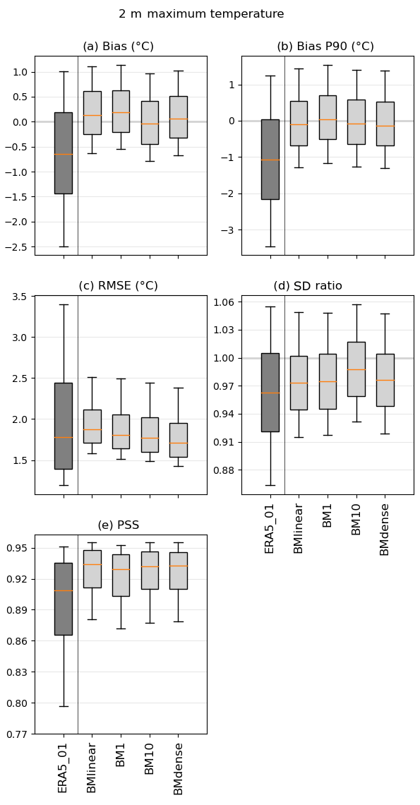
Figure 5 Error measures of the DL downscaling of ERA5 for daily maximum temperature (2010–2014) in relation to the Iberia01 observations. The errors considered are bias, bias of the 90th percentile, root mean square error (RMSE), standard deviation ratio (SDR), and Perkins' skill score (PSS). As reference, the errors in ERA5 interpolated to 0.1^∘ are also shown. Each box plot represents the value of all grid points of the output of each CNN model forced with ERA5. The box represents the interval between the 25th and 75th percentiles. The orange line is the median value, and the lower (upper) whisker represents the 10th (90th) percentile.

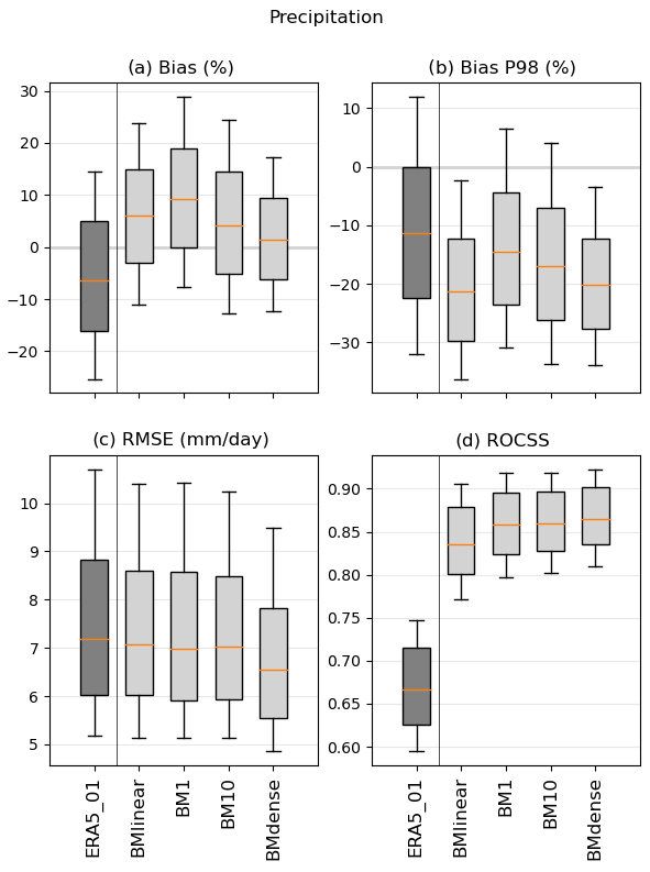
Figure 6 Error measures of the DL downscaling of ERA5 for daily precipitation (2010–2014) in relation to the Iberia01 observations. The errors considered are bias, bias of the 98th percentile, root mean square error (RMSE), and relative operating characteristic skill score (ROCSS). As reference, the errors in ERA5 interpolated to 0.1^∘ are also shown. Each box plot represents the value of all grid points of the output of each CNN model forced with ERA5. The box represents the interval between the 25th and 75th percentiles. The orange line is the median value, and the lower (upper) whisker represents the 10th (90th) percentile.

3.2 Evaluation of DL forced by the ESGCMs

In this section, the error metrics comparing the DL downscaling of the CMIP6 ESGCMs and Iberia01 are displayed for the four analyzed variables (T, T_min, T_max and Pr) and evaluated in the context of the baseline dataset errors, like the CMIP6 ESGCMs at 1^∘ and ERA5 (interpolated at both 1 and 0.1^∘, henceforth iERA5-1 and iERA5-0.1 or simply iERA5). Note that, for each DL downscaled ESGCM, a four-member ensemble, comprising the results from the four DL architectures, is considered.

In general, for T (Fig. 7), the DL ESGCMs show a much better performance in comparison to the ESGCMs, even with regard to the ERA5, at 0.1^∘. All biases for the DL ESGCM results are around zero and show small variabilities (below 0.3 ^∘C). The forcing ESGCMs display both positive and negative median values for the three biases (total, 2nd, and 98th percentiles), ranging in general between −1 and 2 ^∘C, but some rise to 3 ^∘C. The medians for iERA5 are generally closer to zero (below 0.3 ^∘C). Regarding the RMSE, the DL downscaled ESGCMs show similar values, below 0.5 ^∘C, while the iERA5 values are typically below 1 ^∘C, and most of the ESGCMs reach almost 4 ^∘C, except for MIROC6, which exceeds this threshold. The SDR of all models is around 1; nevertheless, the DL ensembles for each ESGCM present less variability. Finally, the PSS metric shows that the DL ESGCMs are able to represent the Iberia01 PDFs remarkably well, yielding scores above 0.93. The ESGCMs display median PSS values between 0.8 and 0.9 and are characterized by large variability.

Considering T_min (Fig. 8), the biases for the DL ESGCMs results are around zero (ranging no more than 0.5 ^∘C), while the forcing ESGCMs and iERA5 show mainly positive values, with medians reaching 4.5 and 2 ^∘C, respectively. The error variability range for the DL ESGCMs is considerably smaller than for the ESGCMs counterparts. For the extreme T_min values (10th percentile), a similar pattern is visible; however, there are slightly greater biases for the ESGCMs. Regarding RMSEs, the DL ESGCM ensemble shows a great improvement with values around 1 ^∘C, whereas the medians of ESGCMs and ERA5 exceed 4 ^∘C and reach ∼ 2 ^∘C, respectively, accompanied by much larger variability ranges. In terms of SDR, all DL downscaling medians are near 1 and with rather small interquartile ranges when compared with ESGCMs and iERA5, reaching 0.3 units. Finally, the PSS metric consistently reveals the added value of the DL ensemble in representing the PDFs with values ∼ 0.94 that compare with values in the range of 0.70 and 0.87 of the ESGCMs.

Regarding T_max (Fig. 9), the DL ensemble shows a clear improvement with regard to the forcing ESGCMs, with median biases less than −0.2 ^∘C, compared with a general underestimation of median values that reach 4 ^∘C for T_max and its 90th percentile. The MIROC6 is the only model overestimating T_max in ∼ 1 ^∘C. The RMSE values display a striking reduction given by the DL approaches, with median RMSE values ranging from 4 and 1.5 ^∘C to less than 0.5 ^∘C. The SDRs are closer to 1 than the ESGCM counterparts and iERA5. Considering the PSS, similarly to what was previously shown, the DL downscaled inter-member variability ranges between 0.92 and 0.97, contrasting with the forcing ESGCMs and iERA5 (although the median PSS values for iERA5 are also high at above 0.9).

Finally, for precipitation (Fig. 10), the performance of the DL ensembles for each ESGCM is less remarkable than for temperatures. Nevertheless, the DL downscaling outperforms the forcing counterparts in all the error metrics, presenting lower errors and variability ranges. Biases, both for Pr and its 98th percentile, point to a general underestimation, ranging between −25 % and 10 %, yet corresponding to much lower overall differences in comparison to Iberia01 than the ESGCMs and iERA5. For the RMSE, the DL ESGCMs and iERA5 are relatively equivalent, with median values of about 10 mm d⁻¹. However, the ESGCM RMSEs show values above 70  mm d⁻¹ but with medians between 18 and 35  mm d⁻¹. A similar behavior is identifiable for the ROCSS, with good results for both the DL ESGCMs and iERA5, with most median values above 0.95, while the ESGCMs median ROCSS values are in the range of 0.7 and 0.9 and extreme values reach −0.2. In contrast, the PSS values of the DL downscaled ESGCMs show lower values, with medians around 0.5, which are smaller than the ∼ 0.72 of the ESGCMs. In some sense, this is not that surprising since we are comparing the ESGCM and Iberia01 precipitation at 1^∘, which has a much smoother spatial pattern than at 0.1.

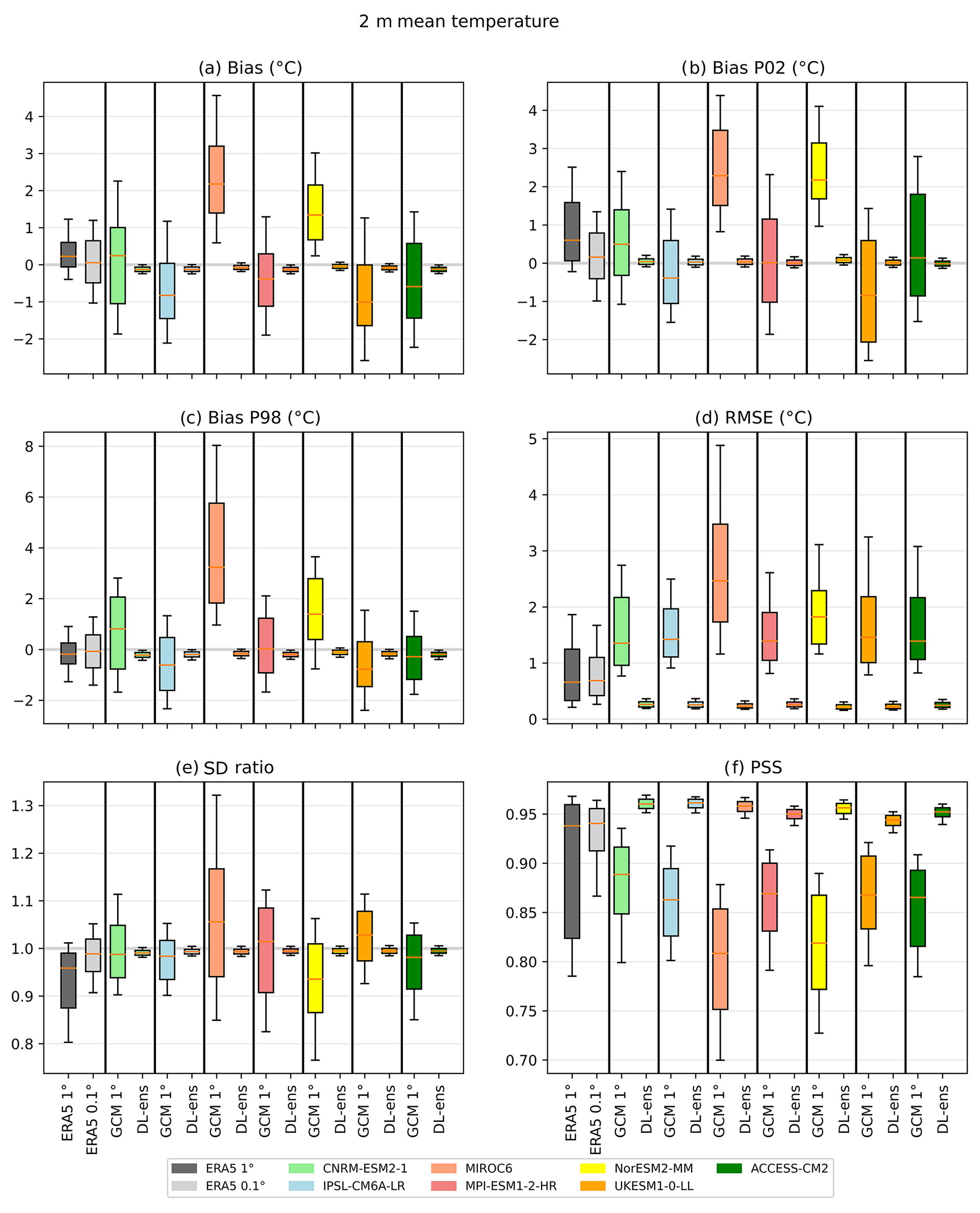
Figure 7 Error measures of the DL downscaling of CMIP6 ESGCMs for daily mean temperature (1979–2014) in relation to the Iberia01 observations. The errors considered are bias, bias of the 2nd and 98th percentile, root mean square error (RMSE), standard deviation ratio (SDR), and Perkins' skill score. As reference, the errors in ERA5 interpolated to 1 and 0.1^∘ and the errors in CMIP6 ESGCMs at 1^∘ are also shown. Each box plot represents the value of all grid points of the output of all CNN models pooled together and forced with each CMIP6 ESGCM. The box represents the interval between the 25th and 75th percentiles. The orange line is the median value, and the lower (upper) whisker represents the 10th (90th) percentile.

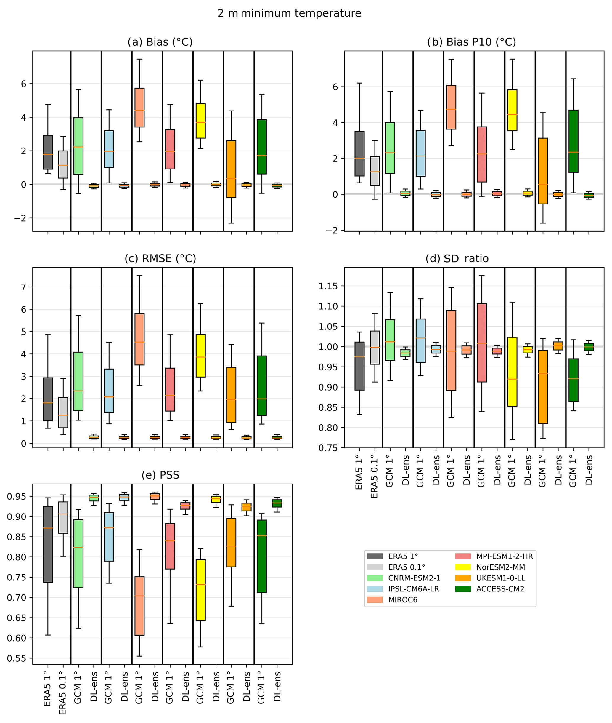
Figure 8 Error measures of the DL downscaling of CMIP6 ESGCMs for daily minimum temperature (1979–2014) in relation to the Iberia01 observations. The errors considered are bias, bias of the 10th percentile, root mean square error (RMSE), Perkins' skill score (PSS), and standard deviation ratio (SDR). As reference, the errors in ERA5 interpolated to 1 and 0.1^∘ and the errors in CMIP6 ESGCMs at 1^∘ are also shown. Each box plot represents the value of all grid points of the output of all CNN models pooled together forced with each CMIP6 ESGCM. The box represents the interval between the 25th and 75th percentiles. The orange line is the median value, and the lower (upper) whisker represents the 10th (90th) percentile.

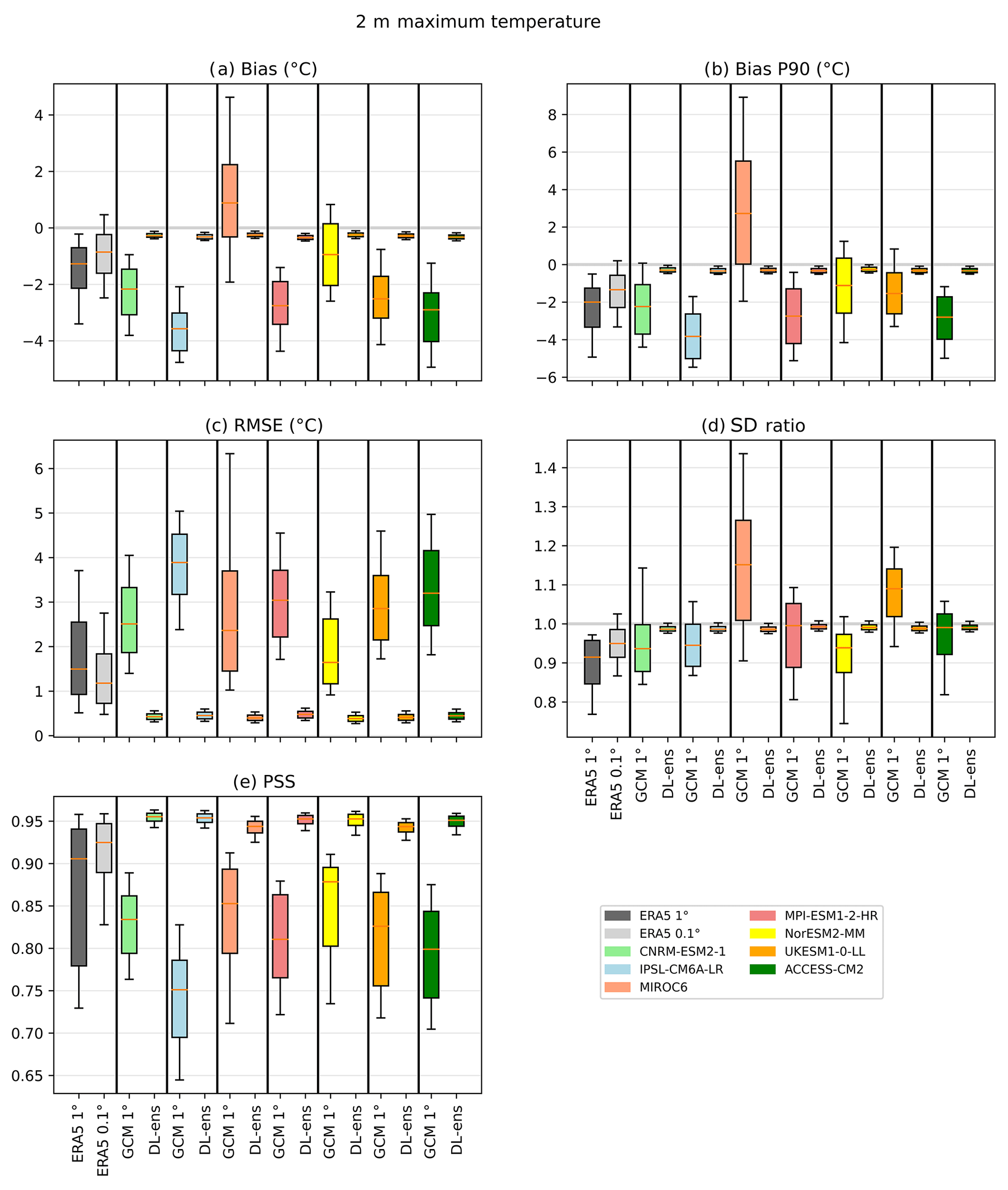
Figure 9 Error measures of the DL downscaling of CMIP6 ESGCMs for daily maximum temperature (1979–2014) in relation to the Iberia01 observations. The errors considered are bias, bias of the 90th percentile, root mean square error (RMSE), standard deviation ratio (SDR), and Perkins' skill score. As reference, the errors in ERA5 interpolated to 1 and 0.1^∘ and the errors in CMIP6 ESGCMs at 1^∘ are also shown. Each box plot represents the value of all grid points of the output of all CNN models pooled together and forced with each CMIP6 ESGCM. The box represents the interval between the 25th and 75th percentiles. The orange line is the median value, and the lower (upper) whisker represents the 10th (90th) percentile.

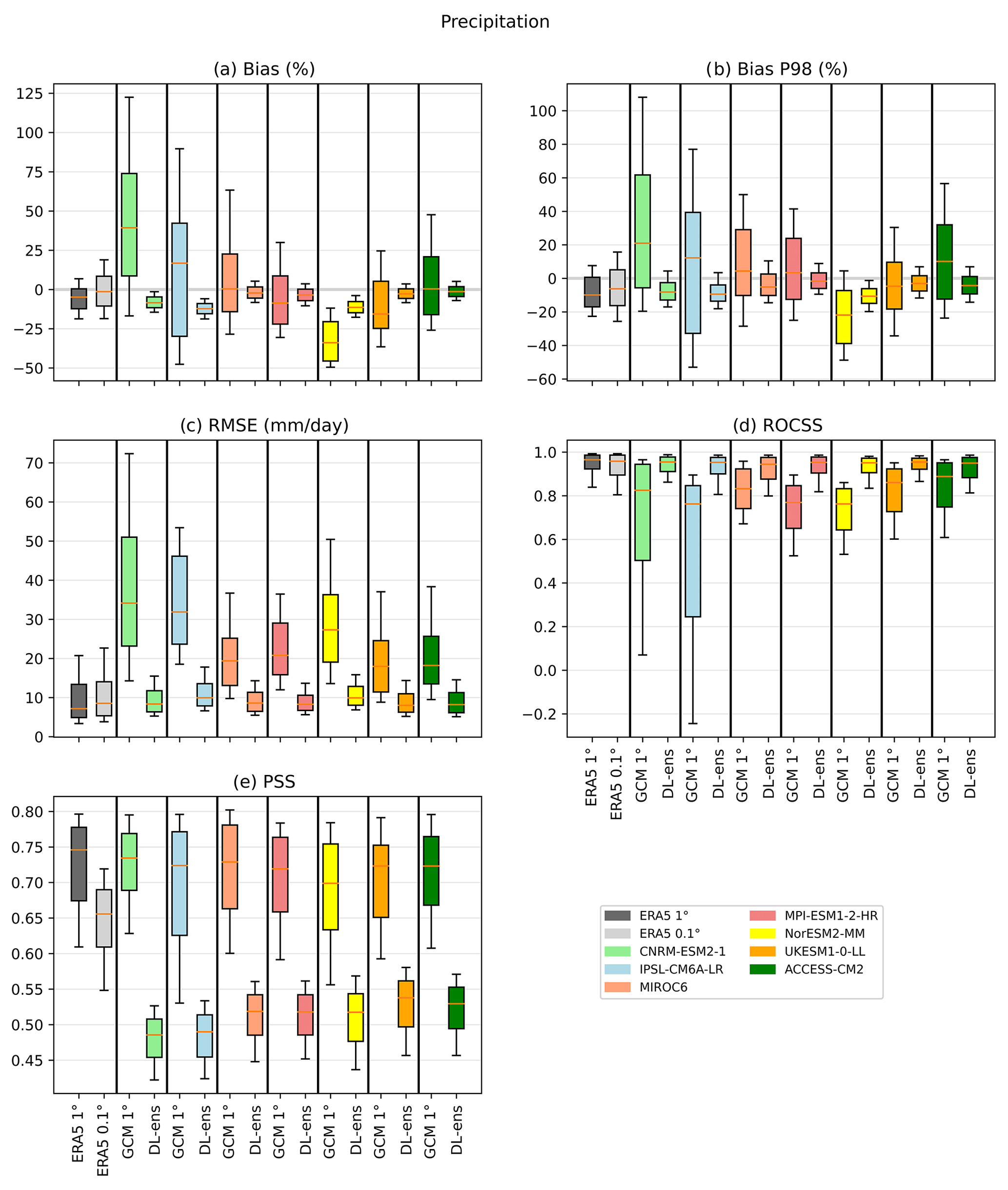
Figure 10 Error measures of the DL downscaling of CMIP6 ESGCMs for daily precipitation (1979–2014) in relation to the Iberia01 observations. The errors considered are bias, bias of the 98th percentile, root mean square error (RMSE), Perkins' skill score, and relative operating characteristic skill score (ROCSS). As reference, the errors in ERA5 interpolated to 1 and 0.1^∘ and the errors in CMIP6 ESGCMs at 1^∘ are also shown. Each box plot represents the value of all grid points of the output of all CNN models pooled together and forced with each CMIP6 ESGCM. The box represents the interval between the 25th and 75th percentiles. The orange line is the median value, and the lower (upper) whisker represents the 10th (90th) percentile.

3.3 Iberian future mean climate

The evaluation of the ability of the DL architectures to downscale both the ERA5 and the ESGCMs during the historical climate provided the necessary confidence to apply this method to downscale the future ESGCMs climate simulations. Therefore, here, the projected changes from the DL downscaled ESGCM ensemble are shown, as obtained from the comparison of three future time slices (2015–2040, 2041–2070, and 2071–2100) with the 1981–2010 historical period, in terms of anomalies (i.e., future minus historical). The four SSP–RCP pairs are analyzed (SSP1–2.6, SSP2–4.5, SSP3–7.0, and SSP5–8.5) for each of the four variables. The simple-averaged unweighted ensembles were built considering all ESGCMs and DL architectures. Therefore, the DL ESGCM ensembles are composed of 28 members (seven models times four architectures). Figures 11 to 14 refer to the projections for T, T_min, T_max and Pr, respectively. If fewer than two-thirds of the ESGCMs members agree on the change signal, then the grid point is signalized with a gray dot, which reveals the lack of robustness of the projected change. A spatial comparison between the projected changes from the 1^∘ ESGCMs ensemble, the 0.1^∘ DL downscaled ESGCM ensemble, and the interpolated version of the latter, at 1^∘ (to offer a fair comparison with the original datasets), is conducted to highlight the differences and added value brought by the DL downscaled ensembles.

The future projected changes for T are displayed in Fig. 11 for the forcing 1^∘ ESGCMs (labeled “1^∘ GCM” in the panels) and for the DL downscaled ESGCM ensemble (labeled “DL-MM_01” in the panels) for the three future time slices under the four scenarios. Overall, the results show a projected increase in T, starting from the 2015–2040 period and continuing towards the end of the 21st century (Fig. 11a). Naturally, the SSP1–2.6 (SSP5–8.5) scenario depicts the smallest (greatest) changes. Under SSP1–2.6, projected changes of up to 2.5 ^∘C are discernible, and the patterns exhibit analogous characteristics when comparing the ensemble of ESGCM to the downscaled ensembles generated using DL (Fig. 11a). This similarity is also evident in the remaining scenarios, although with the additional advantage of DL downscaled ESGCM ensembles displaying more detailed patterns of warming. Both DL and ESGCM ensembles demonstrate temperature increases of up to 1.5, 3.5, and 6 ^∘C during the periods 2015–2040, 2041–2070, and 2071–2100, respectively, under the SSP5–8.5 scenario. But the corresponding median warming values for Iberia are around 1.23, 2.5, and 5 ^∘C. In the case of SSP2–4.5 and SSP3–7.0, there is less pronounced warming, although it may still reach up to 3.5 and 4.5 ^∘C, respectively. These results are more easily observed by condensing the spatial information into box plots (Fig. 11b). Overall, differences between DL and ESGCM ensemble are more pronounced from the middle of the century onwards, especially for the two worst-case scenarios (SSP3–7.0 and SSP5–8.5).

Considering T_min (Fig. 12), the results present similar features to those from T. Within SSP1–2.6, projected changes between 0.5 and 2 ^∘C are visible, with more pronounced warming in the end of the century. The behavior is similar between the ESGCM ensemble and the downscaled one. Local variations in the patterns of T_min projected changes are visible for all time slices and scenarios in the outcomes from the DL downscaled ensemble, which is compatible with the results from higher-resolution models and able to describe local phenomena in greater detail (contrary to a simple interpolation method). For the SSP5–8.5 scenario, results for the 2041–2070 (2071–2100) period are similar between ensembles, with projected increases from 2 to 3.5 ^∘C (3 to 5.5 ^∘C). Note, however, that the DL ensemble projects local increases of up to 6 ^∘C in the central Iberian Peninsula, which are not present in the ESGCM ensemble projections. This behavior is also depicted in the box plots of Fig. 12b.

T_max (Fig. 13) presents similar characteristics to T and T_min. At the beginning of the 21st century (2015–2040), the magnitude of the projections from both the ESGCM and DL ensemble ranges from 0.5 to 2 ^∘C in most of the Iberian Peninsula (Fig. 13a), independently of the scenario. In the mid-21st century (2041–2070), projections from both the ESGCM and DL downscaled ensembles represent a similar range of projected changes (up to 3.5 ^∘C, depending on the scenario; Fig. 13b). By 2071–2100, warming values are almost 2-fold those of the middle of the century, surpassing 6.5 ^∘C in the worst-case scenario. It should be highlighted that the DL downscaled ensemble shows different areas of extreme projected increases in T_max (towards south) that are not present in the ESGCM ensemble (where the largest warming is found towards more central and northeastern regions).

Figure 14 shows the Pr projected changes for the future time slices and scenarios, which, in this case, consider the mean daily accumulated values and their changes (in  mm d⁻¹). In contrast, the changes depicted in Fig. 14 are rather different from the ones in Figs. 11 to 13. While the ESGCM ensemble projects a rather homogeneous decrease in the mean daily precipitation for all future periods and scenarios, the DL downscaled ensemble shows mostly consistent decreases in the western and northern areas of Iberia and non-robust regional increases throughout central and eastern Iberia, independently of the period and scenario. It is important to emphasize that most of these projected increases are not robust (i.e., fewer than two-thirds of the ensemble members agree on the signal), whereas almost all projected decreases are robust (Fig. 14a). Negative Pr projections are found mainly in the northern, western, and southwestern portions of Iberia, increasing in area and robustness towards 2100 and with the SSP5–8.5 scenario. These features are in overall agreement with the ESGCM ensemble; nevertheless, there is much increased detail due to the enhanced horizontal resolution. In fact, for the 2071–2100 time slice under the SSP5–8.5, the ESGCM (DL downscaled) ensemble shows projected decreases of down to −0.75  mm d⁻¹ (−1  mm d⁻¹ in the northern and northwestern Iberia). The box plots in Fig. 14b are largely affected by the compensating effect of different signal projected changes, resulting in overall larger ranges of projected change (even for the interpolated DL ensemble, at 1^∘) and median values closer to zero, in comparison with the ESGCM ensemble. Nonetheless, an overall decrease in the Iberian precipitation is visible in that the one for the DL ensemble is smaller than the one shown by the forcing ESGCM ensemble.

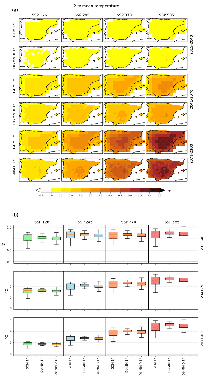
Figure 11 Mean temperature relative changes given by the DL CMIP6 ESGCM multi-model ensemble at 0.1^∘ for SSP1–2.6, SSP2–4.5, SSP3–7.0, and SSP5–8.5 (2015–2040, 2041–2070, 2071–2100 minus 1981–2010)/1981–2100. (a) Maps. Gray dots specify grid points where fewer than two-thirds of the DL CMIP6 ESGCM pairs agree on the change signal (no occurrences). (b) Box plots. The DL CMIP6 ESGCM multi-model ensembles were interpolated to 1^∘, and the results are also displayed. As reference, the change signal linked to the ESGCM ensemble at 1^∘ is also shown in panels (a) and (b). Each box plot represents the value of all grid points of the output of all CNN models pooled together and forced with all CMIP6 ESGCMs pooled together. The box represents the interval between the 25th and 75th percentiles. The orange line is the median value, and the lower (upper) whisker represents the 10th (90th) percentile.

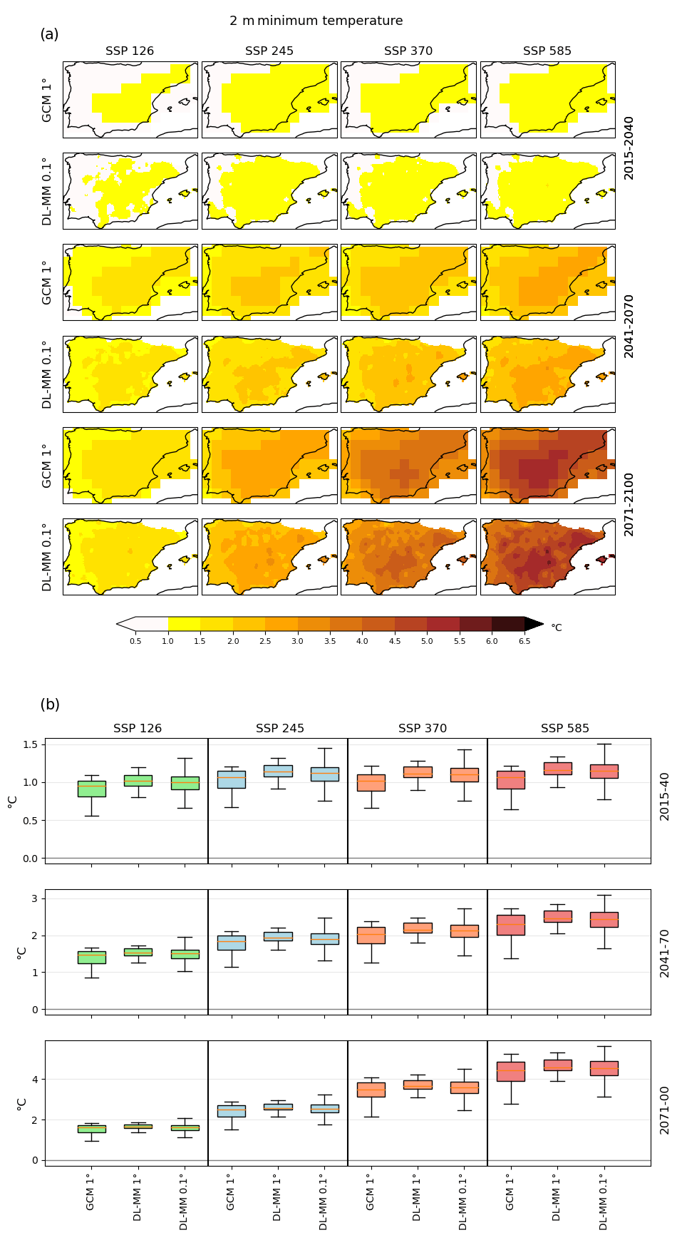
Figure 12 Minimum temperature relative changes given by the DL CMIP6 ESGCM multi-model ensemble at 0.1^∘ for SSP1–2.6, SSP2–4.5, SSP3–7.0, and SSP5–8.5 (2015–2040, 2041–2070, 2071–2100 minus 1981–2010)/1981–2100. (a) Maps. Gray dots specify grid points where fewer than two-thirds of the DL CMIP6 ESGCM pairs agree on the change signal (no occurrences). (b) Box plots. The DL CMIP6 ESGCM multi-model ensembles were interpolated to 1^∘, and the results are also displayed. As reference, the change signal linked to the ESGCM ensemble at 1^∘ is also shown in panels (a) and (b). Each box plot represents the value of all grid points of the output of all CNN models pooled together and forced with all CMIP6 ESGCMs pooled together. The box represents the interval between the 25th and 75th percentiles. The orange line is the median value, and the lower (upper) whisker represents the 10th (90th) percentile.

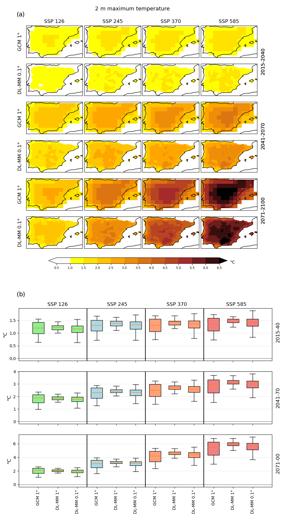
Figure 13 Maximum temperature relative changes given by the DL CMIP6 ESGCM multi-model ensemble at 0.1^∘ for SSP1–2.6, SSP2–4.5, SSP3–7.0, and SSP5–8.5 (2015–2040, 2041–2070, 2071–2100 minus 1981–2010)/1981–2100. (a) Maps. Gray dots specify grid points where fewer than two-thirds of the DL CMIP6 ESGCM pairs agree on the change signal (no occurrences). (b) Box plots. The DL CMIP6 ESGCM multi-model ensembles were interpolated to 1^∘, and the results are also displayed. As reference, the change signal linked to the ESGCM ensemble at 1^∘ is also shown in panels (a) and (b). Each box plot represents the value of all grid points of the output of all CNN models pooled together and forced with all CMIP6 ESGCMs pooled together. The box represents the interval between the 25th and 75th percentiles. The orange line is the median value, and the lower (upper) whisker represents the 10th (90th) percentile.

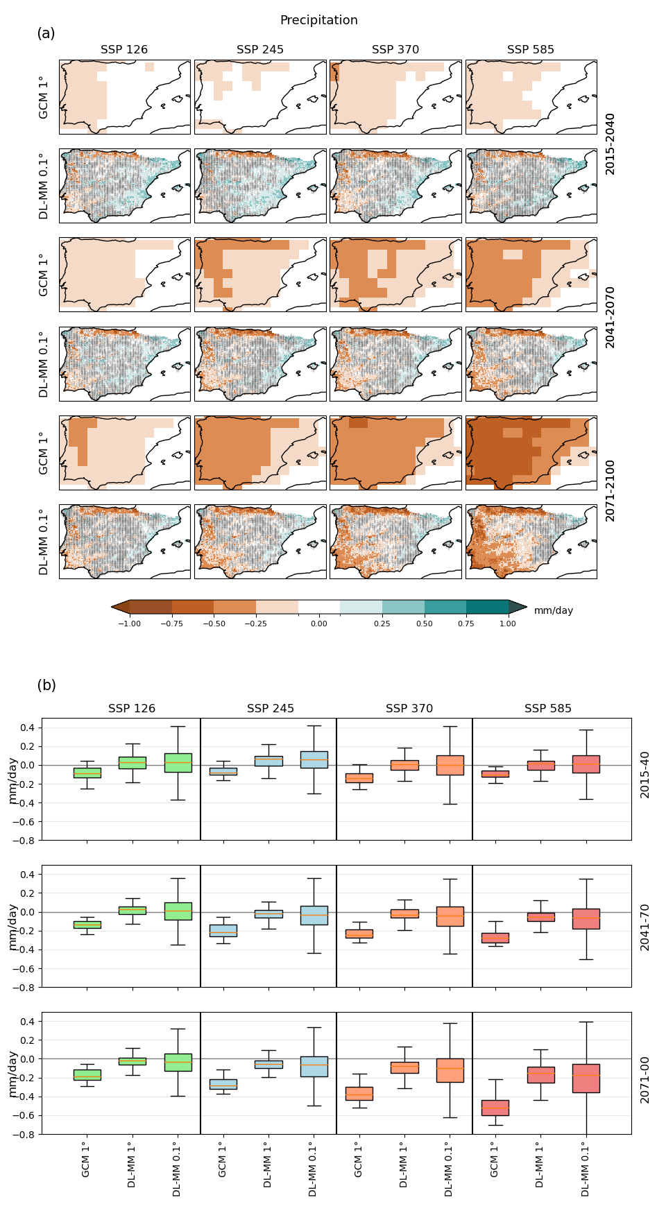
Figure 14 Daily mean precipitation relative changes given by the DL CMIP6 ESGCM multi-model ensemble at 0.1^∘ for SSP1–2.6, SSP2–4.5, SSP3–7.0, and SSP5–8.5 (2015–2040, 2041–2070, 2071–2100 minus 1981–2010)/1981–2100. (a) Maps. Gray dots specify grid points where fewer than two-thirds of the DL CMIP6 ESGCM pairs agree on the change signal (no occurrences). (b) Box plots. The DL CMIP6 ESGCM multi-model ensembles were interpolated to 1^∘, and the results are also displayed. As reference, the change signal linked to the ESGCM ensemble at 1^∘ is also shown in panels (a) and (b). Each box plot represents the value of all grid points of the output of all CNN models pooled together and forced with all CMIP6 ESGCMs pooled together. The box represents the interval between the 25th and 75th percentiles. The orange line is the median value, and the lower (upper) whisker represents the 10th (90th) percentile.

3.4 Iberian future climate extremes

Considering climate extremes, in this section, the projected changes in the three climate extreme indices are compared for both the ESGCM and the DL downscaled ESGCM ensembles, similar to Sect. 3.3. For T_min and T_max, the 10th and 90th percentiles were considered, respectively, while, for the extreme precipitation, the 95th percentile of the daily mean accumulated values was computed.

In general, the future 10th percentile of T_min (Fig. 15) reveals lower warming projections than for T_min (Fig. 12) and also different patterns. The most pronounced warmings are located in the south-central and eastern regions of Iberia (Fig. 14a), which may reach 2 ^∘C (4 ^∘C) in the 2041–2070 (2071–2100) period for the SSP5–8.5 scenario. The remaining scenarios show lower warmings, reaching 1.5, 2.5, and 3.5 ^∘C for SSP1–2.6, SSP2–4.5, and SSP3–7.0, respectively, by the end of the century. As expected, the warming patterns are much more detailed and localized when the DL ensemble is considered.

Similar to extreme T_min, the projections of extreme T_max (Fig. 16) exhibit comparable patterns to those of the mean climate variable (Fig. 13), although with much more pronounced warming values. In particular, over a significant portion of Iberia, the warming reaches over 8 ^∘C by the end of the century for the SSP5–8.5 scenario. The use of a precise and performance-evaluated technique to downscale a large ensemble of ESGCM climate projections at a high resolution provides substantial added value in capturing local climate change for the 90th percentile of T_max, as demonstrated in Fig. 16a. For instance, when considering the 2071–2100 period under SSP5–8.5, both the ESGCM and DL downscaled ensembles project changes exceeding 8 ^∘C. However, the DL downscaled ensemble surpasses this threshold over a wider area, locally exceeding 9 ^∘C and even extending to the southern coast of Iberia, where the projections from the ESGCM ensemble do not surpass 6 ^∘C.

Regarding the extreme Pr (Fig. 17), the DL projections point to reductions in the extreme precipitation across southwestern Iberia, expanding eastward (for part of southern Iberia) throughout the 21st century, and more pronounced for the SSP3–7.0 and SSP5–8.5 scenarios. These decreases can reach more than 3 mm d⁻¹ in these regions. On the other hand, essentially over central, southeastern, and northwestern Iberia, DL projections show an intensification in extreme precipitation in all scenarios and time periods, reaching increases that surpass 3 mm d⁻¹. The ESGCMs projections mostly present decreases in extreme precipitation (for all time slices and scenarios, except the SSP1–2.6 during 2015–2040 and 2041–2070 in the northern half of the peninsula; Fig. 17a). The spatial pattern of changes in extreme precipitation are dissimilar for the DL and ESGCMs projections. The box plots in Fig. 17b summarize the differences between the ESGCM and DL downscaled ensembles, being, nevertheless, slightly affected by the lack of robustness of some of the outcomes, as the DL ensemble shows a larger variability than the ESGCM ensemble.

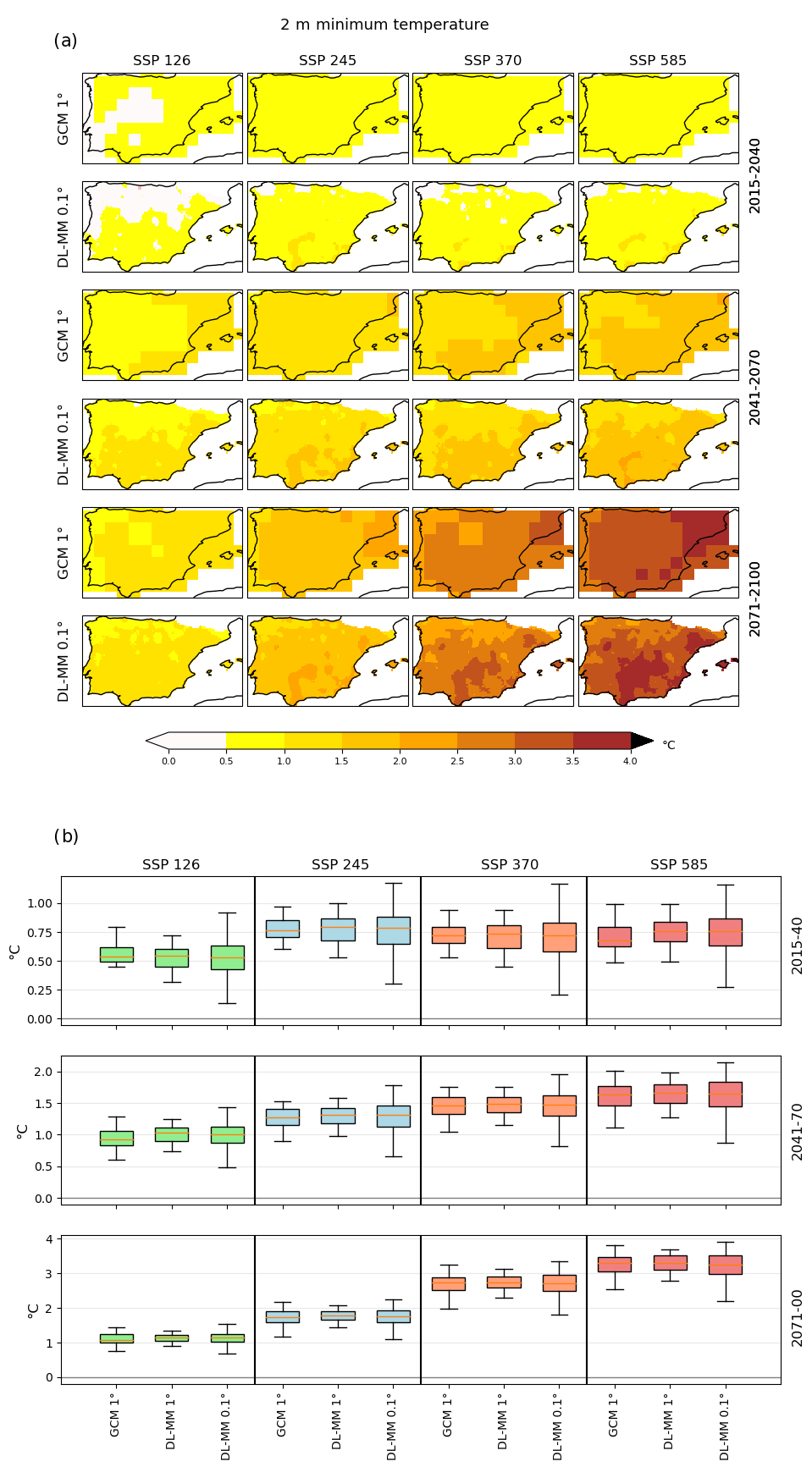
Figure 15 Mean minimum temperature 10th percentile relative changes given by the DL CMIP6 ESGCM multi-model ensemble at 0.1^∘ for SSP1–2.6, SSP2–4.5, SSP3–7.0, and SSP5–8.5 (2015–2040, 2041–2070, 2071–2100 minus 1981–2010)/1981–2010. (a) Maps. Gray dots represent grid points where fewer than two-thirds of the DL CMIP6 ESGCM pairs agree on the change signal (no occurrences). As reference, the change signal linked to all ESGCMs at 1^∘ is also shown. (b) Box plots. Each box plot represents the value of all grid points of the output of all CNN models pooled together and forced with all CMIP6 ESGCMs pooled together. The box represents the interval between the 25th and 75th percentiles. The orange line is the median value, and the lower (upper) whisker represents the 10th (90th) percentile.

Figure 16 Mean maximum temperature 90th percentile relative changes given by the DL CMIP6 ESGCM multi-model ensemble at 0.1^∘ for SSP1–2.6, SSP2–4.5, SSP3–7.0, and SSP5–8.5 (2015–2040, 2041–2070, 2071–2100 minus 1981–2010)/1981–2010. (a) Maps. Gray dots represent grid points where fewer than two-thirds of the DL CMIP6 ESGCM pairs agree on the change signal (no occurrences). As reference, the change signal linked to all ESGCMs at 1^∘ is also shown. (b) Box plots. Each box plot represents the value of all grid points of the output of all CNN models pooled together and forced with all CMIP6 ESGCMs pooled together. The box represents the interval between the 25th and 75th percentiles. The orange line is the median value, and the lower (upper) whisker represents the 10th (90th) percentile.

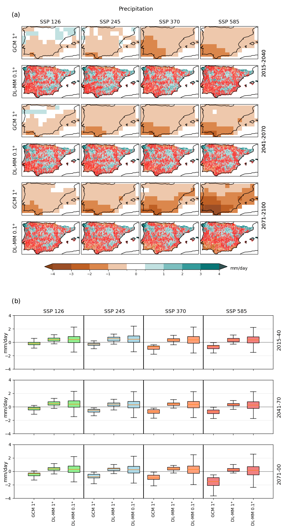
Figure 17 Precipitation 95th percentile relative changes given by the DL CMIP6 ESGCM multi-model ensemble at 0.1^∘ for SSP1–2.6, SSP2–4.5, SSP3–7.0, and SSP5–8.5 (2015–2040, 2041–2070, 2071–2100 minus 1981–2010)/1981–2010. (a) Maps. Red dots represent grid points where fewer than two-thirds of the DL CMIP6 ESGCM pairs agree on the change signal. As reference, the change signal linked to all ESGCMs is also shown. (b) Box plots. Each box plot represents the value of all grid points of the output of all CNN models pooled together and forced with all CMIP6 ESGCMs pooled together. The box represents the interval between the 25th and 75th percentiles. The orange line is the median value, and the lower (upper) whisker represents the 10th (90th) percentile.

4 Discussion and conclusions

The Iberian Peninsula, situated in the southwestern tip of the European continent within the Mediterranean region is considered a climate change hotspot, due to the projected future warming and drying conditions. These changes can significantly impact the natural environment and human health in the region (Giorgi, 2006; Soares et al., 2017a, b; Cramer et al., 2018; Lionello and Scarascia, 2018; Cardoso et al., 2019; Tuel and Eltahir, 2020; Soares and Lima, 2022; Lima et al., 2023a, b; Soares et al., 2023a). Consequently, there is an urgent need for accurate climate information to assist the planning and development of adaptation strategies. Recent climate change studies focusing on the Iberian Peninsula relied on RCM simulations forced by CMIP5 GCMs (Soares et al., 2017a, b; Cardoso et al., 2019; Lima et al., 2023a, b; Soares et al., 2023a) to project future climate change with increased resolution, accounting for regional features not captured by coarse ESGCMs. However, following the release of the improved CMIP6 global climate simulations and projections (in the context of the most recent IPCC report, AR6; IPCC, 2021), the need for an updated climate change assessment in the Iberia Peninsula arose. The new high-resolution CMIP6 EURO-CORDEX regional climate simulations and projections will become available within the next 1–2 years. In the interim, however, there is a need for high-resolution climate information to accurately assess future projections over Iberia. In this context, an opportunity emerges to explore alternative approaches to downscale the current CMIP6 simulations and projections. Therefore, this study leverages innovative AI methods to evaluate the evolution of mean, minimum, and maximum temperatures, as well as precipitation, across the Iberian Peninsula, throughout the 21st century. The analysis is based on a multi-model, multi-architecture ensemble of CNN-based downscaled projections derived from CMIP6 ESGCMs. The investigation encompasses three distinct future time slices (2015–2040, 2041–2070, and 2071–2100) in line with four SSP–RCP scenarios of SSP1–2.6, SSP2–4.5, SSP3–7.0, and SSP5–8.5.

First, the ability of four DL architectures to reproduce the historical T, T_min, T_max, and Pr climates was evaluated over Iberia during 2010–2014 (Figs. 3 to 6). During this period, all DL architectures, trained using ERA5 data between 1979 and 2004, revealed a good agreement with observations (Iberia01) for the predictand variables (using solely the predictors as input data). Although more complex architectures, such as BMdense, revealed better performance for Pr (lower overall biases and RMSEs and higher ROCSS), a clear distinction between architectures was not meaningful. The results showed that during the 1979–2014 historical period, the DL downscaled ESGCMs were able to represent the Iberia01 reference climate with large increased performance in comparison with the forcing ESGCMs, even when compared with the ERA5 and iERA5 datasets (Figs. 7 to 10). For Pr, nevertheless, the downscaled error metrics were shown to be similar to the reanalysis ones, despite greater differences in the overall variable distributions (as shown by the PSS values). Such disagreement could be related to the singular behavior of Pr, especially considering its extreme events, which can occur under distinct atmospheric synoptic patterns (predictor sets), thus becoming challenging for the DL architectures to establish empirical relationships between the vertical atmospheric structure and surface-level precipitation accumulation. Overall, the evaluation of the DL downscaled ESGCMs showed a rather good performance in representing the historical climate (mean, minimum, and maximum temperatures and precipitation), providing the necessary confidence to project the future climate change under different scenarios using this new approach. It should be noted that the DL models trained with predictors from ERA5 were used to generate the ESGCMs output for the historical and future periods. The bias correction procedure applied to the ESGCM predictors is an important asset that may allow their values to better agree with those from ERA5. As a result, we believe that the relationship between the predictors of both ERA5 and ESGCMs and Iberia01 are comparable.

The DL downscaled T projections revealed a projected increase between 1 and 1.5 ^∘C over Iberia (Fig. 11), for all scenarios, during the earliest future period (2011–2040). By the end of the 21st century, however, the DL ensemble projected changes were shown to become more heterogeneous between scenarios and generally varied between 1.5 ^∘C (SSP1–2.6) and 5 ^∘C (SSP5–8.5). In all instances, the DL downscaled T projected changes showed a strong agreement with the original CMIP6 ESGCM ensemble in both the signal and main spatial patterns of climate change. Nevertheless, regional-to-local features are clearly enhanced by the increased resolution. In fact, the most poignant difference between the DL and the original ensembles is the horizontal discretization. Local differences can be identified in the most inland areas of the Iberian Peninsula in the DL results, which are not captured by the original ESGCMs, due to the coarse grid that neglects valleys and other geographically enclosed areas, thus fostering greater horizontal heterogeneities. Similar features were found for T_min (Fig. 12) and T_max (Fig. 13) and for the respective extreme values (10th percentile of T_min and 90th percentile of T_max in Figs. 15 and 16, respectively). Between those, T_max showed larger projected increases than T_min (approximately 2-fold), revealing greater intra-daily temperature ranges to be expected in the future. For the extreme T_max values, even under the SSP1–2.6 “optimistic” scenario, DL downscaled projections revealed increases exceeding 3 ^∘C by the end of the 21st century. For the “less optimistic” ones (SSP3–7.0 and SSP5–8.5), extreme T_max projected changes of up to 7 ^∘C were shown for most of Iberia (Fig. 16). DL downscaled projections for extreme T_min, on the other hand, were shown to be higher in the eastern and southern Iberia (Fig. 15), locally surpassing 3.5 ^∘C (for 2071–2100 under SSP5–8.5). Overall, these projections are aligned with the EURO-CORDEX ensemble projections for Iberia (Soares et al., 2017a; Cardoso et al., 2019; Lima et al., 2023a; Amblar et al., 2017) but with small value differences, which are also linked to the dissimilarities regarding the emission scenarios.

The significance of DL downscaling techniques in the context of Pr projections unveiled further intricacies when compared to T, T_min, and T_max projections. Given that the behavior of daily mean accumulated precipitation is heavily influenced by local topography and other phenomena, particularly owing to convective processes, which can result in local, large precipitation accumulations, projecting Pr was shown to be more complex for DL downscaling methods, considering the widespread continental, mountainous areas of the Iberian Peninsula. Therefore, for both Pr (Fig. 14) and extreme Pr (95th percentile; Fig. 17), the original and DL downscaled ESGCM ensemble projections showed greater discrepancies. While the ESGCM projected changes showed essentially negative values, corresponding to the future large-scale expected drying over Iberia, the DL results revealed a drying trend in western and southwestern regions of Iberia, which are stronger for the upper-end scenarios, and local projected increases, mostly in the central and eastern continental regions. The southern and western precipitation reductions are consistent, with a significant reduction in the large-scale precipitation from frontal activity, due to the northern displacement of the storm tracks (Tamarin and Kaspi, 2017). In fact, the northward expansion of the Hadley cell lead to a northward shift in the storm tracks over the North Atlantic, resulting in a reduction in the large-scale precipitation across southern and western Iberia (Bengtsson et al., 2006; Harvey et al., 2014; Kang and Lu, 2012; Ulbrich et al., 2008). The projected local increases in the precipitation, although non-robust, mostly with fewer than two-thirds of ensemble members in agreement, may be consistent with local-to-regional changes in convective precipitation that are not captured by the original ESGCMs, highlighting potential applications of DL techniques to long-term projections (or even short-term forecasting).

The projected changes in the warming and drying over Iberia, as reported in recent studies using previous CMIP outputs (CMIP5) and in the most recent IPCC report (IPCC, 2021), are consistent with the multi-model, multi-scenario, and multi-architecture DL downscaled ESGCM ensemble projections presented in this study. This behavior is also in accordance with the resulting DL climate change signals from the Baño-Medina et al. (2022) report for Iberia, which showed similar spatial patterns to those obtained from the CMIP5 RCMs but with local-to-regional added value. Previous research has demonstrated that the warming and drying trends over Iberia are more pronounced under high anthropogenic emission scenarios, reflecting the influence of human activities on climate change, compared to the natural variability in the climate system. Our results demonstrated that in the CMIP6 context, within the new set of scenarios encompassing socioeconomic and representative concentration pathways, AI-based DL methods are able to accurately simulate the historical Iberian climate and produce high-resolution scenario-based projections, consistent with each other and with previous studies, using (coarse) GCM forcing and a high-resolution training database. Thus, the present study highlighted the substantial advantages of employing novel approaches based on DL to obtain efficiently up-to-date, high-resolution climate information at a local scale that is specifically for Iberia. This is crucial for supporting and designing mitigation and adaptation strategies.