the Creative Commons Attribution 4.0 License.
the Creative Commons Attribution 4.0 License.
 | 20 Mar 2024
CD-type discretization for sea ice dynamics in FESOM version 2
Carolin Mehlmann
Dmitry Sidorenko
Qiang Wang
Two recently proposed variants of CD-type discretizations of sea ice dynamics on triangular meshes are implemented in the Finite-VolumE Sea ice–Ocean Model (FESOM version 2). The implementations use the finite element method in spherical geometry with longitude–latitude coordinates. Both are based on the edge-based sea ice velocity vectors but differ in the basis functions used to represent the velocities. The first one uses nonconforming linear (Crouzeix–Raviart) basis functions, and the second one uses continuous linear basis functions on sub-triangles obtained by splitting parent triangles into four smaller triangles. Test simulations are run to show how the performance of the new discretizations compares with the A-grid discretization using linear basis functions. Both CD discretizations are found to simulate a finer structure of linear kinematic features (LKFs). Both show some sensitivity to the representation of scalar fields (sea ice concentration and thickness). Cell-based scalars lead to a finer LKF structure for the first CD discretization, but the vertex-based scalars may be advantageous in the second case.
- Article
(3462 KB) - Full-text XML
- BibTeX
- EndNote


The emergence of several global ocean models formulated on unstructured (triangular or hexagonal) meshes, such as the Finite-VolumE Sea ice–Ocean Model (FESOM) (Wang et al., 2014; Danilov et al., 2017), MPAS-Ocean (Ringler et al., 2013; Petersen et al., 2019) and ICON-O (Korn, 2017), triggered the development of sea ice models tailored to such meshes. Very recently, the sea ice components of FESOM (FESIM; Danilov et al., 2015), MPAS-Ocean (MPAS-Seaice; Turner et al., 2022 and Capodaglio et al., 2022) and ICON-O (Mehlmann and Korn, 2021; Mehlmann and Gutjahr, 2022) have been documented. FESIM (Danilov et al., 2015) is based on the finite element method and the piecewise linear P1−P1 collocated discretization. In this case, the discrete sea ice velocities and scalar quantities (concentration and thickness) are placed at mesh vertices, and the discrete fields are assumed to be linear functions on triangles. This is an example of an A-grid discretization, in the terminology of Mehlmann et al. (2021). The original formulation of MPAS-Seaice of Turner et al. (2022) follows the B-grid discretization. In this case, the discrete sea ice velocities are placed at the vertices of the hexagons, and scalars are placed at the hexagon centers. This corresponds to the cell (triangle) placement of the velocity and the vertex placement of the scalars on dual triangular meshes. Several variants of discretization are proposed by Turner et al. (2022), based either on variational principles or on the finite volume method. The new MPAS-Seaice variational discretization developed by Capodaglio et al. (2022) places sea ice velocity vectors at mesh edges. The same staggering is used by Mehlmann and Korn (2021) to discretize the sea ice module of ICON-O on triangular meshes. The discretization by Mehlmann and Korn (2021) uses linear nonconforming (Crouzeix–Raviart) finite elements, while the approximation by Capodaglio et al. (2022) uses either Wachspress (Dasgupta, 2003) or piecewise linear (PWL) representation on sub-polygons into which the mesh cells are additionally subdivided. The discretizations with velocity at the edges are called CD-grid discretizations (Mehlmann et al., 2021).
On triangular meshes, the A, B and CD placements of the discrete sea ice velocity result in different numbers of discrete degrees of freedom (DOF), with a ratio of . The CD placement implies 3 times more degrees of freedom than the A-grid discretization used by FESOM (Danilov et al., 2015) and thus finer effective resolution. An elementary Fourier analysis of the accuracy of the discrete stress divergence operator on triangular A, B and CD grids (see Danilov et al., 2022) also shows that the accuracy correlates with the number of DOF. This is the main motivation for considering CD-type discretizations for sea ice dynamics. However, the numerical efficiency, robustness and the ability to resolve sea ice leads of a particular placement depend on the implementation details.
This paper presents the new implementation of two CD-grid discretizations in the sea ice component of FESOM. Both are based on the standard Hibler viscous–plastic (VP) rheology (Hibler, 1979) and use the modified elastic–viscous–plastic (mEVP) method (Bouillon et al., 2013; Kimmritz et al., 2015). The first, hereafter referred to as CD1, follows Mehlmann and Korn (2021) but is formulated in longitude–latitude coordinates. This formulation includes additional metric terms but does not need to transform velocities between local tangent coordinate systems (Mehlmann and Gutjahr, 2022). CD1 discretization is based on the nonconforming linear (Crouzeix–Raviart) finite elements. These elements require stabilization when applied to problems with full stress divergence (Falk, 1991). The stabilizing term in the sea ice momentum equation used by Mehlmann and Korn (2021) is similar to that proposed in Hansbo and Larson (2003). The strength of the stabilization is well defined in the case of the VP method but requires adjustments in the case of the mEVP method.
The second CD-grid discretization, referred to as CD2, is similar to that used by Capodaglio et al. (2022), but it differs in a systematic finite element derivation based on piecewise linear basis functions defined on sub-triangles obtained by splitting the mesh triangles into four equal smaller triangles and the reconstruction of velocities at vertex locations based on edge velocities. The option of Capodaglio et al. (2022) using the Wachspress basis is not pursued. Some other (minor) differences are due to our use of locally flat triangles.
We use the test case proposed by Mehlmann et al. (2021) to compare the performance of the CD1 and CD2 discretizations and the existing A-grid discretization of FESOM. In fact, the results of FESOM simulations based on CD1 were already presented in Mehlmann et al. (2021), but the description of the implementation in FESOM was missing. Since CD discretizations use 3 times more discrete velocities than the A grid, we also compare the performance of CD1 and CD2 discretizations with the performance of a finer A grid.
The following sections describe main equations (Sect. 2), the implementation and the Fourier analysis (Sect. 3), and test simulations (Sect. 4). They are followed by Discussion (Sect. 5) and Conclusions (Sect. 6).
The sea ice momentum equation is written as
Here, is the total mass of ice and snow per unit area, with ρice and ρs the sea ice and snow densities and hice and hs the respective mean thicknesses (volumes per unit area). Cd is the ice–ocean drag coefficient, ρo is the water density, aice is the sea ice concentration, and uo are the sea ice and ocean velocities, τ is the wind stress applied to sea ice, H is the sea surface elevation, g is the acceleration due to gravity, and is the force from the internal stresses in ice (Hibler, 1979),
where
is the strain rate tensor; η and ζ are the viscosities,
I is the identity matrix, and P0 is the ice strength. Here, and are the components of the symmetric tensor in Eq. (3) with respect to the orthogonal basis given by unit zonal (with index 1) and meridional (with index 2) vectors and
The default parameters are e=2, C=20, s−1 and N m−2. Δmin regularizes plastic behavior if Δ is very small, replacing it with a viscous flow. To suppress sea ice motion in the absence of forcing, the last term in Eq. (2) contains an additional factor (after P0), i.e., the replacement pressure (Hibler and Ip, 1995).
The modified elastic–viscous–plastic method (mEVP) is used to solve for the sea ice dynamics in the same form as in Danilov et al. (2015) and Koldunov et al. (2019b). This method is a reformulation of the original EVP method described by Hunke and Dukowicz (1997), and it is preferred here because it removes the association of the sub-cycling time step of the standard elastic–viscous–plastic method with numerical stability (Lemieux et al., 2012; Bouillon et al., 2013; Kimmritz et al., 2015). The stability is governed by additional dimensionless parameters, α and β. The product αβ should be sufficiently large compared to (Bouillon et al., 2013; Kimmritz et al., 2015) for numerical stability of the iterative procedure. Even though the number of iterations, NEVP, should be formally larger than α, β to ensure convergence to VP, it has been demonstrated by, e.g., Kimmritz et al. (2017) and Koldunov et al. (2019b) that much smaller NEVP is often sufficient in practice. Simulations reported below use NEVP=100, and α, β are adjusted to ensure stability for the resolution and discretization used.
3.1 Spherical geometry
In the discretization of the sea ice momentum equation, spherical geometry is taken into account similarly to Danilov et al. (2015) and is consistent with Turner et al. (2022) and Capodaglio et al. (2022), apart from some modifications due to the weak formulation in our case and the approximation of locally flat triangles (vs. tangent plane). We use longitude–latitude coordinates (ϕ, θ). In realistic applications, these coordinates are those of a rotated coordinate system with the “North Pole” displaced to Greenland. The rotation necessitates the transform of forcing and redefines the Coriolis parameter but has no other implication for the numerical method. To simplify the description, the rotation of the coordinate system is ignored in the following. The distances Δx and Δy on mesh triangles are computed with respect to the first triangle vertex using the value of cosine at triangle center as Δx=Recos θcΔϕ and Δy=ReΔθ. The index c implies that the quantity is related to the cell (i.e., triangle), and Re is Earth's radius. These distances are used to compute arrays of vertex or edge weights that define derivatives in zonal and meridional directions on triangles (see Sect. 3.2 and 3.3). Additional metric terms appear in computations of strain rates and in computations of stress divergence. They are specified below. Apart from these additional metric terms and cosines used in computations of relative distances and derivatives, all other computations look as if the geometry were flat. Therefore, we use ∂x and ∂y to denote spatial derivatives as defined in and local Cartesian coordinates on triangles. Under this convention the previously introduced indices 1 and 2 in Eq. (4) are x and y. The FESOM simulations described below are carried out using a flat geometry which is achieved by setting the values of cos θc to 1 and the metric factor to zero. The cosines and metric factors are stored in arrays which are filled before the time stepping, so switching between flat and spherical geometries does not affect the code.
3.2 Case CD1: a CD discretization based on nonconforming linear finite elements
For brevity, we will begin with the VP momentum, Eq. (1) and then explain the modifications needed for the mEVP method. The momentum equation is first projected on some sufficiently smooth test functions, w. The internal stress is integrated by parts to obtain a weak formulation,
Here, R combines all other terms except for those that are explicitly written, and the colon implies a tensor product. The sea ice velocity is approximated by a series in nonconforming (Crouzeix–Raviart) linear basis functions,
Here, the summation is over all mesh edges, and Ne(x,y) is the nonconforming linear basis function. It is equal 1 on edge e and varies linearly to −1 on the vertex v opposite to edge e. In Fig. 1, on edge e1, is 0 at mid-points of edges e2 and e3, and is −1 at v1, and similarly on the other triangle opposite to the yellow one. Ne is zero outside two triangles sharing edge e. Note that the nonconforming basis function coincides with the standard linear function defined on a small triangle formed by connecting mid-edge points and then continued to the primary triangle. For this reason, if the set of triangle edges is ordered so that e1 is opposite to v1 of the set of triangle vertices (see Fig. 1), the derivatives of Ne can be obtained from the derivatives (already available in the FESOM sea ice module) of standard linear basis functions by multiplication with −2. A lumped approximation is used for R,
We will further suppress the upper index h used to denote discrete approximations. The components of strain rate tensor are written as
where is the metric factor. To simplify computations, we approximate metric terms by constants on triangles. The discrete strain rates on triangle c become
They are constant on triangles. Here, E(c) is the set of edges of triangle c.
The stresses are also considered to be constant on triangles, which requires that the ice strength P0 is constant too. If the scalar degrees of freedom are placed on cells, which is one option in our implementation, the discrete P0 is constant on triangles without additional approximations. If scalar fields are linear on triangles with the discrete degrees of freedom on vertices, as in Danilov et al. (2015), which is the second option here, P0 is computed at the central quadrature point, i.e., using mean aice and hice on triangles. Note that because the concentration aice enters the exponent in P0 (Eq. 5), this may reduce P0 in places where the concentration varies strongly.
The next step is to obtain the Galerkin approximation. The above polynomial approximations are inserted in Eq. (6), and the test function is taken as , where j is the edge index and wj is an arbitrary weight vector. The equations for sea ice velocity are obtained by requiring that the result holds for any wj. However, since the nonconforming function Ne(x,y) is discontinuous at edges other than e (except for mid-points), one restricts the integration to triangle interiors and adds penalty (stabilization) terms that effectively connect the triangles:
As shown by Hansbo and Larson (2003) (see also Mehlmann and Korn, 2021), the stabilization term is
where C is an order 1 constant; le is the length of edge e; [q] is the jump of quantity q across the edge; and ζe is the estimate of viscosity ζ on edge e, which is taken as mean over triangles sharing e.
The nonconforming functions are orthogonal on elements, so for and is zero otherwise. The edge value of mass is obtained as half the sum of two vertex or two cell values depending on the discretization of scalar fields. The computations of the third and fourth terms on the left-hand side of Eq. (10) are similar to the computations in Danilov et al. (2015), but we repeat them here for completeness. In spherical geometry, there are metric terms in ∇Nj, leading to
The metric contributions initially contained Nj, which left after integration over the cell area. Note that, compared to the case when the stresses are differenced directly, some metric terms are absent in the weak formulation. The reason is that they originate from the differentiation of cos θ, which is hidden in dSc in Eq. (11). Even if we used a linear representation for cos θ on triangle c, the result would be the mean cosine on the triangle (absorbed in Sc on the right-hand side of Eq. 11) because stresses are constant on triangles for linear basis functions.
Computations of ∇H in the fourth term on the left-hand side of Eq. (10) do not involve differentiation of metrics. In FESOM, H is known at vertices. The mass at edge j, as above, is the mean of two vertex values for the vertex-based scalars and two cell values for the cell-based scalars. The result is
where , Mv is the standard linear basis function on triangle c and V(c) is the set of vertices of triangle c.
The integration over edges in the stabilization term involves so that le drops out of the final result. The stabilization term is computed through two cycles over triangles, similar to Mehlmann and Korn (2021). The first cycle collects the contributions from the velocity on the triangle into the edge velocity differences, and the second one adds these contributions to the equations for edge j. The presence of the stabilization term is critical. As shown by the elementary Fourier analysis (Danilov et al., 2022), there is no approximation for the eigenvalues of discrete divergence of stresses if this term is absent.
The extension of this discretization to the mEVP method requires empirical adjustment of the strength of the stabilization. The point is that stresses in this method are iterative EVP approximations to the VP stresses. The stabilization term is the contribution to the stress divergence, and it does not appear in the iterative sub-cycling of stresses in the mEVP method. It has been empirically found that the stabilization pre-factor has to be essentially smoother than of the VP method and that its amplitude has to be tuned for numerical stability of the mEVP method. Instead of 2Cζe we take , where is the area associated with the edge (with c1 and c2 the triangles sharing the edge). C is dimensional in this case and is taken as C=2.5 s2 m−2. Apart from the intention to make stability of iterative process less sensitive to Δt and changes in mesh resolution, the selection is purely empirical. It was tested in the range of resolutions of 2–8 km in computations reported in Mehlmann et al. (2021) but may need additional tuning in other situations. A VP implementation can be a safer way to proceed with the stabilization, but it is not pursued in this work as we employ the EVP or mEVP methods in our practical applications.
As mentioned above, both vertex (P1) and cell representations of scalar fields are supported in the sea ice code. In the first case we use the FCT-FEM method of Löhner et al. (1987), as described in Danilov et al. (2015), to advect the tracers. Because of the use of consistent mass matrices, its high-order part is nominally fourth order in space and second order in time. For the cell-wise constant scalars we use the first-order upwind method, which will be replaced by an FCT method with the second-order high-order part for practical applications in the future.
3.3 Case CD2: a CD-grid discretization with conforming linear elements on sub-triangles
The difference from the previous (CD1) case lies in the selection of basis and test functions. Consider triangle c with vertices and edges , as shown in Fig. 1. As mentioned above, the convention is that e1 is opposite to v1, and so on. The notation e1,e2 and e3 for edges will be also used to denote the mid-edge points, which should not lead to ambiguities. By connecting the mid-edge points, each primary mesh triangle is subdivided into four smaller triangles. Triangle c in Fig. 1 is subdivided into triangles and s4 with the following ordering of vertices: for s1, for s2, for s3 and for s4. The ordering is important, because it allows us to use the array of derivatives computed for the primary triangle. The velocity field is assumed to be linear on each sub-triangle. We store the derivatives of standard linear basis functions Mv, v∈V(c) for each c as matrices and . The derivatives of linear functions on sub-triangles, by virtue of the ordering described above, are obtained by multiplication of these matrices with −2 for s1 and 2 for s2,s3 and s4 for given c. Note that, compared to the nonconforming linear basis functions of the previous section, only the representation on sub-triangle s1 remains the same.
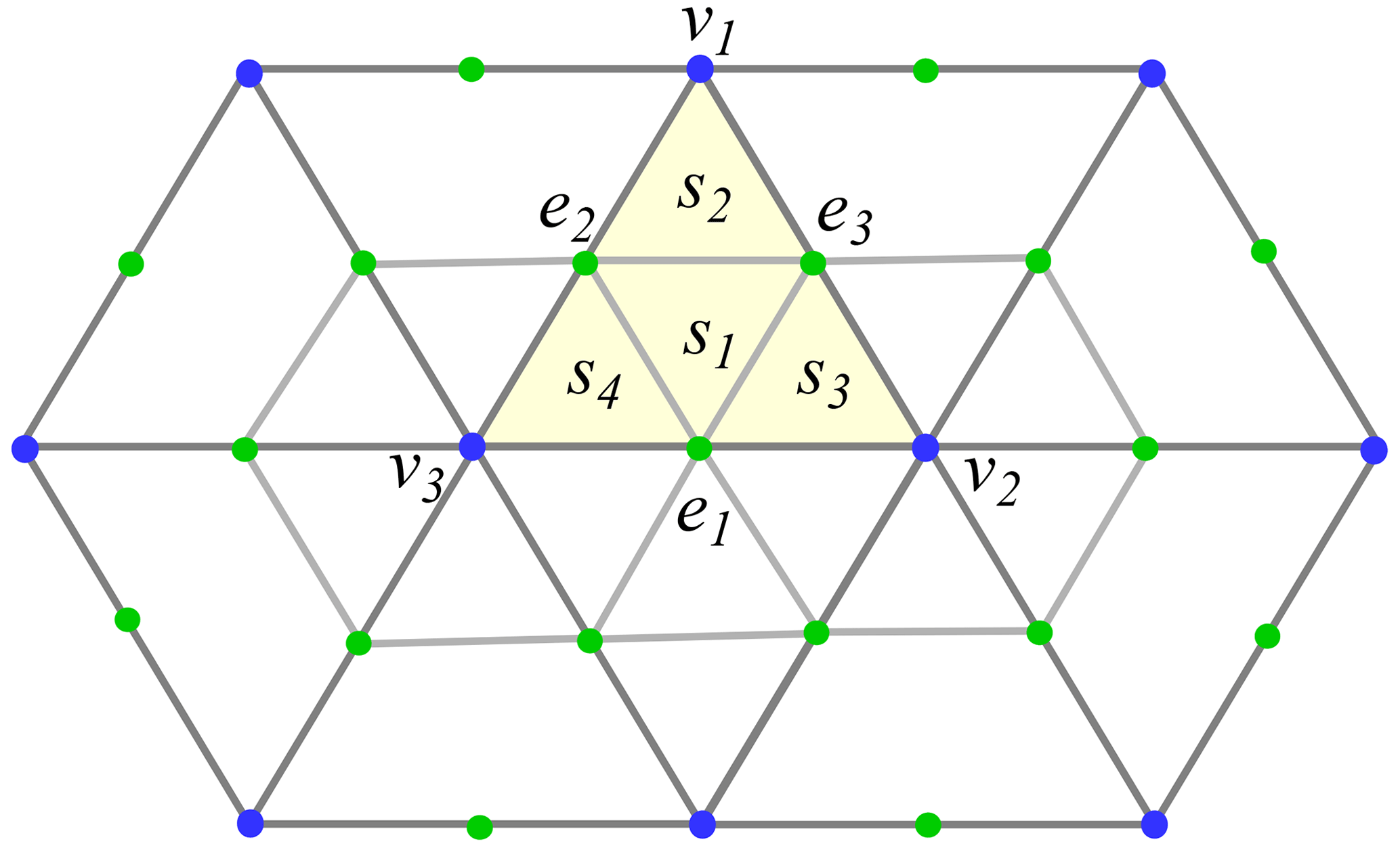
Figure 1CD1: the nonconforming linear function on the yellow triangle equals 1 on edge e1, −1 at v1, and 0 on the line connecting the mid-points of e2 and e3. CD2: triangle c (shaded yellow) is split into four sub-triangles ( and s4) by connecting mid-edge points. The set of triangle edges (edge mid-points) is ordered such that they are opposite to triangle vertices . The basis function at e1 is non-zero at the set of sub-triangles that meet at e1, v2 or v3. This basis function equals 1 at e1, at v2 and at v3, where and are scalar weights in Eq. (13). It decays linearly to 0 at all other green points of the stencil.
The available degrees of freedom are associated with edge velocities, same as in the previous section. The edge velocity is interpreted as a mid-edge value. Values of velocity at mesh vertices are reconstructed as a weighted mean of edge velocities,
The weights are normalized so that for each v. They are first taken as inverse of edge length and then normalized. This reconstruction rule and the linear representation on sub-triangles imply that for each edge e we are working with a piecewise linear basis function Ne which equals 1 at the mid-point of e, goes linearly to 0 at other edge mid-points in triangles sharing e, goes linearly to Wve at the edge vertices and goes linearly to 0 at mid-points of other edges joining at vertices. The support of in Fig. 1 is the combination of sub-triangles meeting at e1 or v2 or v3.
In terms of Ne thus defined, the velocity field is written as
In practice, we use two separate arrays: one to store the resolved velocities ue and another one to store their vertex reconstructions uv. In the same way as for the CD1 discretization, the strain rates are assumed to be constant on sub-triangles, and the metric terms are approximated by constants to achieve this. The ice strength is taken as constant on primary triangles, which leads to stresses that are constant on sub-triangles. Since there are four sub-triangles in each triangle c, 4 times more discrete stresses are iterated in the mEVP procedure. This increases computational load compared to the case of nonconforming functions, where the computation cycle is limited to the primary triangles of the mesh.
To obtain the Galerkin approximation, the test function is taken to be any of Nj=wjNj. Since Nj is now continuous, no additional penalty terms are present (in contrast to the CD1 discretization of the previous section), and for edge j we get
In the terms with the time derivative and Re, ∫NjNedS are the components of mass matrix. In contrast to the case of nonconforming functions, this matrix is not diagonal now. Similar to Danilov et al. (2015), it is replaced by its diagonally lumped approximation for numerical efficiency,
where Se is the row sum of mass matrix entries. It is equal to
where .
The computations of the third and fourth terms on the left-hand side of Eq. (14) are done in the double cycle over triangles (external) and sub-triangles (internal). Each term is computed as explained above for the case of nonconforming functions, but now the standard P1 functions on sub-triangles are used instead of nonconforming functions. The contributions from the stress divergence from sub-triangles are first collected in auxiliary edge-based (Fe) and vertex-based (Fv) arrays. For example, the sub-triangle s2 in Fig. 1 contributes to the edges e2 and e3 and to the vertex v1. On completing the cycle over triangles, the edge-based result Fe is updated by two vertex-based contributions Fv as
We see that actual basis and test functions Ne are not used in computations. They are, however, needed for the consistent Galerkin formulation, in particular, for defining how to compute Se. The procedure used by Capodaglio et al. (2022) to determine consistent areas associated with edge degrees of freedom is similar to the one used here, but the finite element approach automatically determines the areas associated with the computational nodes. Once again, we note that the presence of sub-triangles increases the computational load in finding the stress divergence.
3.4 Fourier analysis of CD2
It is instructive to perform the Fourier analysis of CD2. It will provide an independent argument on the accuracy of this discretization, similarly to the analysis in Danilov et al. (2022).
Consider an infinite triangular mesh made of equilateral triangles with side length a and height . Let the x axis be directed along one of the triangle sides and the y axis along the height drawn to that side. The discrete velocities are located at mid-edges. For the Fourier analysis they are naturally split into three families related to sides with the same orientation. A degree of freedom associated with a particular side of a triangle has a neighborhood with the stencil which is oriented differently compared to those associated with other sides. This is why one needs to introduce six (three for u and three for v) separate velocity amplitudes in order to perform the Fourier analysis,
Here, the subscript e denotes edges, and Ea, Eb and Ec are the sets containing edges oriented as e1,e2 and e3 (Fig. 1), respectively; is the wave vector; and xe is the location of the mid-edge point of edge e.
A vertex velocity is reconstructed from the edge velocities. The amplitude of vertex velocity is
The cosines contain phase shifts between a vertex and respective mid-edge points of edges emanating from this vertex.
In the same way as in Danilov et al. (2022), the stress divergence operator is linearized, the sea ice strength (and hence the viscosities η and ζ) is taken constant and the geometry is assumed to be flat. One is interested in the eigenvalues of the stress divergence operator . We take to ensure that the eigenvalues are sufficiently close to each other in plots.
We first compute the strain rates on each of the four sub-triangles of a primary mesh triangle (see Fig. 1), counting the phases relative to their centers. For example, for sub-triangle s1, formed by the vertices at e1,e2 and e3, the gradients of basis functions on this triangle are , and , respectively, so that the amplitude of on this triangle is
and similarly for all other strain rate components on sub-triangle s1 and also for the strain rates on other sub-triangles. Note that the expressions for the gradients and phase shifts depend on the orientation of primary triangles. The expression above is valid for triangles that are oriented as the yellow triangle in Fig. 1. For the primary triangles of opposite orientation (the neighbors of the yellow triangle in Fig. 1), the strain rate amplitudes are minus complex conjugates of the respective results for the triangle . In numerical computations this complication is automatically taken into account when the arrays of derivatives are computed. After the strain rates on sub-triangles are computed, the direct stress divergence contributions to edges and vertices are found, and then the edge expressions are updated for vertex contributions, just as is done in numerical computations. The resulting Fourier symbol of discrete stress divergence is a 6-by-6 matrix, the eigenvalues of which are found numerically and plotted in the left panel of Fig. 2.
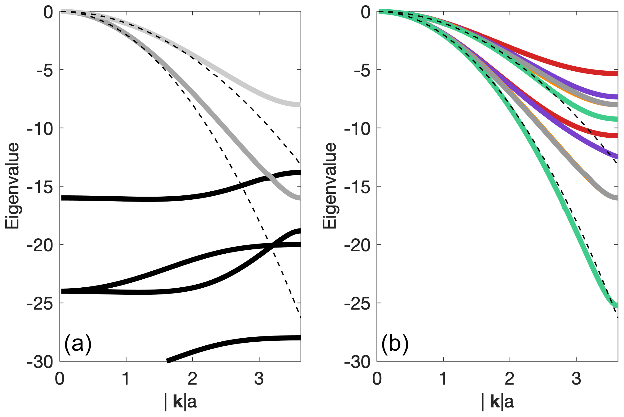
Figure 2(a) The eigenvalues of the (dimensionless) Fourier symbol of (thick gray lines) for the CD2 discretization as a function of dimensionless wavenumber for the wavevector oriented at to the x axis and ζ=η. The thin dashed lines show the dimensionless eigenvalues and of the continuous case. Thick black lines show the spurious branches. (b) Comparison with physical eigenvalues of other discretizations (Danilov et al., 2022). In order of increasing accuracy: A grid (red), B grid (Turner et al., 2022; PWL basis) (magenta), CD2 (gray), CD1 (green). The B grid of FESOM is nearly identical to CD2 and is barely seen (orange cast).
These have to be compared with the eigenvalues of CD1 and other discretizations given in Danilov et al. (2022). As in the case of CD1, there are two physical (thick gray) and four numerical (thick black) branches. The numerical branches are strongly dissipative in the limit of small wavenumbers and do not require any special care. There is no kernel (no zero eigenvalues except for zero wavenumbers), so no stabilization is needed. The right panel of Fig. 2 plots the physical eigenvalues found in Danilov et al. (2022) for other discretizations together with those of CD2 discretization. The range of wavenumbers where the stress divergence eigenvalues give an accurate representation of continuous eigenvalues is noticeably narrower for CD2 than for CD1 discretization. We thus expect to see lower resolving power for CD2 compared to CD1. The eigenvalues of CD2 are more accurate than those of the B-grid discretization of Turner et al. (2022) and the A-grid discretization of FESOM. The Fourier analysis only shows that different discretizations have potentially different accuracy. Full nonlinear simulations are needed to judge their real performance.
Since this work relies on the already existing discretizations, we only compare the performance of the two new CD methods in FESOM with respect to their numerical efficiency and ability to represent linear kinematic features (LKFs) based on the test case proposed by Mehlmann et al. (2021). Their comparison under realistic conditions will be carried out in a separate work. The representation of LKFs is judged qualitatively by their fine structure and quantitatively by computing the number of simulated LKFs using the method of Hutter et al. (2019). CD1 and CD2 discretizations are run in two options with the cell-based and vertex-based scalars. One expects that the ability to represent the fine structure of LKFs is mainly governed by the number of degrees of freedom used to resolve velocities. However, on triangular meshes, the number of cells is twice that of vertices, which may lead to a more detailed representation of sea ice concentration and thickness. Furthermore, computations of mean ice strength on triangles in our implementations imply averaging for the vertex-based scalars to cells, whereas no averaging is applied in the cell-based case. For more details on the influence of the tracer placement on the resolution of LKFs, see Mehlmann and Danilov (2022). We also compare the CD-grid simulations with those performed with the default A-grid sea ice discretization of FESOM on a finer mesh with the same number of degrees of freedom as for the CD discretizations.
The test case is run on a triangular mesh occupying a rectangular domain of 512 by 512 km. Except for western and eastern boundaries, the triangles are equilateral. Smaller rectangular triangles are added along the western and eastern boundaries to make these boundaries straight. The sides of equilateral triangles are 2 km for CD discretizations. The A-grid simulation is run on the mesh with a triangle side of km. The test case describes the initial phase of sea ice deformation under the forcing of a cyclone moving diagonally to the north-eastern corner. Precise formulation of the test case and forcing parameters can be found in Mehlmann et al. (2021). All simulations use the same external time step Δt=2 min. While a larger time step is possible, the selected time step would be typical if the sea ice model were run together with an ocean model at such spatial resolution. The simulated sea ice patterns at the end of the second day of the model integration are compared. We use on the A grid but increase them to 1500 on CD grids to maintain numerical stability. Our other runs (not shown here) indicate that the sensitivity of the simulations to the precise values of α, β is weak if these values are sufficiently large for stability of the iterative procedure. All runs use NEVP=100, as mentioned earlier.

Figure 3Sea ice concentration (a, b) and Δ (c, d) in the test case described by Mehlmann et al. (2021), simulated with CD1 discretization (a, c) and CD2 discretization (b, d) with the cell-based sea ice concentration and thickness.
Figure 3 presents the field of sea ice concentration (top row) and Δ (see Eq. 4) (bottom row) for CD1 (nonconforming basis functions) in the left column and for CD2 (linear basis functions on sub-triangles) in the right column. In both cases the scalars are placed on cells, and the first-order upwind advection is used. It can be seen that CD1 simulates more LKFs. The LKFs are wider and have fewer small-scale details in CD2.
Figure 4 presents the same fields as Fig. 3 in the first two columns but for vertex-based scalars. Here, too, the ability of CD1 to simulate finer scales is clearly seen in both the concentration and Δ. However, by comparison with the patterns of Fig. 3, we conclude that the vertex placement of scalars leads to some reduction in details in the western parts of the domain for CD1, despite the fact that the high-order advection scheme (see Danilov et al., 2015) is used in this case in contrast to the highly dissipative first-order upwind scheme used for the cell-based scalars. For CD2, almost no difference is seen between the cell and vertex placement.
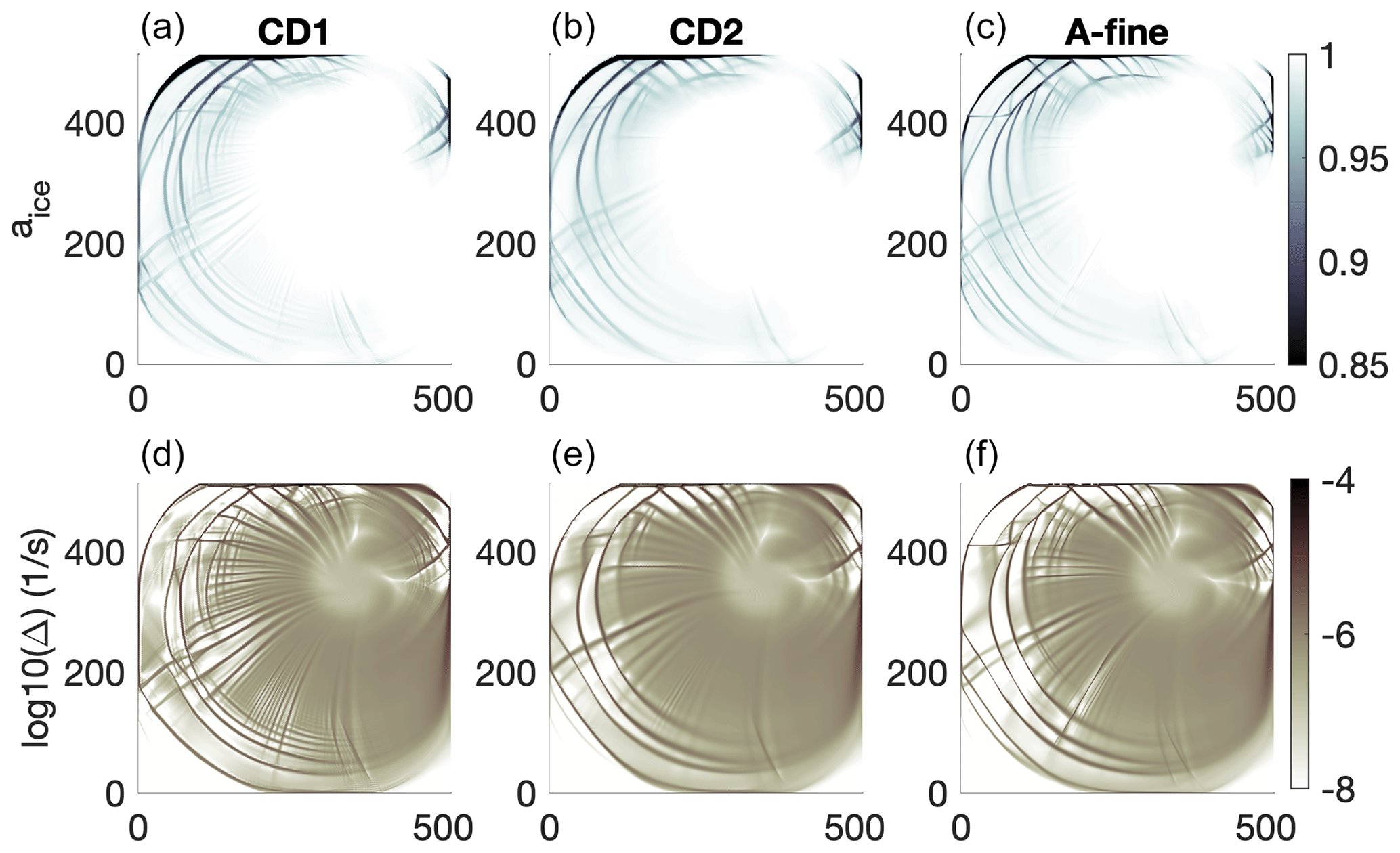
Figure 4Same as in Fig. 3 but for the cases with vertex-based scalars for CD1 discretization (a, d), CD2 discretization (b, e) and fine A-grid discretization (c, f). The two CD cases are for a mesh with a triangle side of 2 km, while the A-grid case is for a mesh with a triangle side of km.
The third column in Fig. 4 displays the sea ice concentration and Δ for the vertex (A-grid) velocity placement but on a finer mesh. The number of velocity degrees of freedom in this case is approximately the same as in the CD cases. Fine scales are better simulated than in the case of CD2 but still less resolved than in the case of CD1. The number of LKFs diagnosed with the algorithm of Hutter et al. (2019) are 114 for the A grid and 73 and 75 for CD2 with cell and vertex scalars, respectively, to be compared with ≈200 for CD1 with cell scalars.
Mehlmann et al. (2023) compare the performance of the CD discretizations in ICON-O, MPAS and FESOM frameworks. They show that the number of LKFs simulated by the FESOM CD2 discretization is lower compared to that simulated in the MPAS framework. Further experiments carried out after the present paper was submitted show that the CD2 discretization is sensitive to the representation of the ice strength for the vertex-based scalars, which correspond to the cell scalars of hexagonal meshes. The ice strength P0 (Eq. 5) in the FESOM implementation was taken constant on primary mesh triangles (e.g., the triangle with vertices v1,v2 and v3 in Fig. 1) in the simulations shown in Fig. 4 and used in Mehlmann et al. (2023). This choice was inherited from the A-grid and CD1 discretizations, where it led to element-wise constant strain rates and stresses. For the CD2 discretization, a more accurate choice is possible for vertex scalars. The ice strength is still element-wise constant but on small triangles. Returning to Fig. 1, P0 is based on the mean thickness and concentration on the triangle only for s1; the values of P0 on triangles s2,s3 and s4 are estimated at vertices v1,v2 and v3, respectively. This treatment increases the number of simulated LKFs (not shown), which becomes closer to that of MPAS simulations. The vertex placement of scalars leads in this case to finer detail than the cell placement, despite the number of DOF for the cell placement being twice as large. This observation indicates that not only the representation of scalars, but also the representation of P0, is important. A detailed analysis is the subject of future work.
The higher resolving capability of the CD (edge) placement of velocity compared to the vertex (A-grid) placement is related to its number of discrete velocities being 3 times as large. The larger number of degrees of freedom implies shorter distances between their locations and may potentially lead to a more accurate approximation of differential operators. The gain in accuracy depends on the discretization, and an elementary Fourier analysis of the eigenvalues of the linearized stress divergence operator in Danilov et al. (2022) and in Sect. 3.3 here indicates that CD1 is more accurate than CD2, and both outperform the A-grid discretization. This result agrees with the behavior of discretizations in the simple test simulations above. We also note that CD1 outperforms the A grid even in terms of LKFs per degree of freedom, as mentioned in Mehlmann and Danilov (2022) and also illustrated above by the A-grid run on a -times-finer mesh.
A caveat of the CD1 discretization is that it needs stabilization to remove kernels in differential operators, as discussed by Mehlmann and Korn (2021). The stabilization constant C requires tuning with the methods of EVP type, and, although the empirically found value ensures reliable work across some tested range of mesh resolutions, it may still need some attention on highly variable meshes. In contrast, CD2 does not require stabilization. From this perspective, it can be viewed as a more robust alternative to CD1.
We also note that CD1 shows a tendency to simulate very close LKFs, separated by several mesh cells. They are well seen in Fig. 3 for cell-based scalars but become less apparent in Fig. 4 for the vertex-based scalars. It is difficult to judge whether such scales are already affected by numerical errors in a full nonlinear case (the accuracy of the linear stress divergence operator remains high for ; see Fig. 2). It remains to be seen which of the two CD discretizations on triangular meshes is more reliable in real-world applications on general unstructured meshes.
In our implementation, CD1 is approximately 2 times and CD2 approximately 4 times more expensive than the A-grid code on the same mesh. In all cases there are two basic cycles over triangles. The stresses are computed in the first cycle, and the divergence of stresses is computed in the second cycle. For the A-grid discretization these two cycles take most of the CPU time. In CD1, there are two additional cycles over triangles to compute the contribution of stabilization, which largely explains the CPU time doubling. The cycles over triangles in CD2 include an inner cycle over four sub-triangles, which is the main reason for the observed increase in the computational load in this case. We speculate that some optimization is still possible, so these numbers can only be treated as preliminary estimates. In addition to the increase in the time needed for computations, the number of halo exchanges in parallel implementation also increases in the CD cases. As compared to the A-grid code, in our implementation the CD1 discretization requires an additional halo exchange for edge velocity differences. The CD2 case needs additional exchanges for vertex velocities and for the contributions to the divergence of stresses that are assembled at vertices. As demonstrated by Koldunov et al. (2019a), the halo exchanges in the sea ice module are the factor limiting the scalability of FESOM in massively parallel applications. This raises a question on the effect of CD discretizations on scalability, which also requires further work.
The A-grid run on a -times-finer mesh, which ensures the same number of degrees of freedom as in the CD cases, is approximately as computationally expensive as CD2. The fact that it simulates more LKFs than CD2 might be related to a much more accurate representation of scalars in this case. However, sea ice simulations are generally run on the surface mesh of the ocean model, and the potential possibility of using a separate finer mesh for sea ice is not always feasible. One would opt for using CD1 or CD2 instead of A-grid discretization if a better resolution of LKFs is required than the one provided by the A grid.
There is a possible extension of CD2 discretization. Instead of considering vertex velocities as dependent variables one treats them as independent ones, in addition to the edge velocities, and uses P1 finite elements on sub-triangles. The scalars are treated as previously on the original mesh. This extension is equivalent to considering the sea ice dynamics on a virtual twice-finer mesh. The increase in the numerical work is negligible compared to the case of CD2 discretization, but the advantage is the smaller support of basis functions, hence better resolution. Also, as follows from the Fourier analysis (the right panel of Fig. 2), the B-grid implementation of FESOM, briefly sketched in Danilov et al. (2022), is nearly as accurate as CD2. It is nearly as expensive as CD1. A detailed comparison of these possibilities in realistic simulations deserves further work.
We describe the implementation of two CD-type discretizations of sea ice mEVP dynamics in FESOM2. They are based on the finite element method and the use of longitude–latitude coordinates. Both discretizations have been proposed earlier by Mehlmann and Korn (2021) (CD1) and Capodaglio et al. (2022) (CD2), respectively. In the first case, the difference to the original implementation lies in using the longitude–latitude coordinates and the addition of metric terms, which eliminates the need to transform velocities between local tangent coordinate systems. In the second case, the difference lies in using the finite element approach, which makes the derivation more compact and automatically determines the surface area associated with the velocity degree of freedom.
Both CD1 and CD2 demonstrate higher LKF-resolving capability than the A-grid discretization. Although CD2 shows lower resolving capacity than CD1, it may be more robust in (m)EVP dynamics as it does not need much additional adjustment. The new discretizations can be sensitive to particular implementation details. It also remains to be seen how these new discretizations behave in realistic global climate simulations compared to the standard A-grid discretization of FESOM, which is the subject of our future work.
The exact version of the model used to produce the results used in this paper is archived on Zenodo (https://doi.org/10.5281/zenodo.7646908; Danilov et al., 2023). The mesh files and data files used to compile the last two figures are archived together with the code (Danilov et al., 2023).
SD worked on the implementation. All the authors contributed to writing and discussion.
At least one of the (co-)authors is a member of the editorial board of Geoscientific Model Development. The peer-review process was guided by an independent editor, and the authors also have no other competing interests to declare.
Publisher’s note: Copernicus Publications remains neutral with regard to jurisdictional claims made in the text, published maps, institutional affiliations, or any other geographical representation in this paper. While Copernicus Publications makes every effort to include appropriate place names, the final responsibility lies with the authors.
We acknowledge the use of the METIS (Karypis and Kumar, 1998) software package for mesh partitioning and express our thanks to N. Hutter for the use of his LKF diagnostics. This paper is a contribution to the project S2, Improved parameterizations and numerics in climate models, of the Collaborative Research Center TRR 181, “Energy transfers in Atmosphere and Ocean”, funded by the Deutsche Forschungsgemeinschaft (DFG, German Research Foundation; project no. 274762653).
The work of Carolin Mehlmann is funded by the Deutsche Forschungsgemeinschaft (DFG, German Research Foundation; project no. 463061012).
The article processing charges for this open-access publication were covered by the Alfred-Wegener-Institut Helmholtz-Zentrum für Polar- und Meeresforschung.
This paper was edited by Philippe Huybrechts and reviewed by Giacomo Capodaglio and one anonymous referee.
Bouillon, S., Fichefet, T., Legat, V., and Madec, G.: The elastic-viscous-plastic method revisited, Ocean Model., 71, 2–12, 2013. a, b, c
Capodaglio, G., Petersen, M. R., Turner, A. K., and Roberts, A. F.: An unstructured CD-grid variational formulation for sea ice dynamics, J. Comput. Phys., 473, 111742, https://doi.org/10.1016/j.jcp.2022.111742, 2023. a, b, c, d, e, f, g, h
Danilov, S., Wang, Q., Timmermann, R., Iakovlev, N., Sidorenko, D., Kimmritz, M., Jung, T., and Schröter, J.: Finite-Element Sea Ice Model (FESIM), version 2, Geosci. Model Dev., 8, 1747–1761, https://doi.org/10.5194/gmd-8-1747-2015, 2015. a, b, c, d, e, f, g, h, i, j
Danilov, S., Sidorenko, D., Wang, Q., and Jung, T.: The Finite-volumE Sea ice–Ocean Model (FESOM2), Geosci. Model Dev., 10, 765–789, https://doi.org/10.5194/gmd-10-765-2017, 2017. a
Danilov, S., Mehlmann, C., and Fofonova, V.: On discretizing sea-ice dynamics on triangular meshes using vertex, cell or edge velocities, Ocean Model., 170, 101937, https://doi.org/10.1016/j.ocemod.2021.101937, 2022. a, b, c, d, e, f, g, h, i
Danilov, S., Mehlmann, C., Sidorenko, D., and Wang, Q.: Sea ice CD-type discretizations of FESOM, Zenodo [code and data set], https://doi.org/10.5281/zenodo.7646908, 2023. a, b
Dasgupta, G.: Interpolants within convex polygons: Wachspress' shape functions, J. Aerospac. Eng., 16, 1–8, https://doi.org/10.1061/(ASCE)0893-1321(2003)16:1(1), 2003. a
Falk, R.: Nonconforming Finite Element Methods for the Equations of Linear Elasticity, Math. Comput., 57, 529–529, 1991. a
Hansbo, P. and Larson, M.: Discontinuous Galerkin and the Crouzeix–Raviart element: Application to elasticity, ESAIM, 37, 63–72, 2003. a, b
Hibler III, W. D.: A Dynamic Thermodynamic Sea Ice Model, J. Phys. Oceanogr., 9, 815–846, 1979. a, b
Hibler III, W. D. and Ip, C. F.: The effect of sea ice rheology on Arctic buoy drift, edited by: Dempsey, J. P. and Rajapakse Y. D. S., ASME AMD, 207, Ice Mechanics, 255–263, ISBN 0791813223, 1995. a
Hunke, E. C. and Dukowicz, J. K.: An Elastic-Viscous-Plastic model for sea ice dynamics, J. Phys. Oceanogr., 27, 1849–1867, 1997. a
Hutter, N., Zampieri, L., and Losch, M.: Leads and ridges in Arctic sea ice from RGPS data and a new tracking algorithm, The Cryosphere, 13, 627–645, https://doi.org/10.5194/tc-13-627-2019, 2019. a, b
Karypis, G. and Kumar, V.: A fast and high quality multilevel scheme for partitioning irregular graphs, SIAM J. Sci. Comput., 20, 359–392, 1998. a
Kimmritz, M., Danilov, S., and Losch, M.: On the convergence of the modified elastic-viscous-plastic method for solving the sea ice momentum equation, J. Comp. Phys., 296, 90–100, 2015. a, b, c
Kimmritz, M., Losch, M., and Danilov, S.: A comparison of viscous-plastic sea ice solvers with and without replacement pressure, Ocean Model., 115, 59–69, 2017. a
Koldunov, N. V., Aizinger, V., Rakowsky, N., Scholz, P., Sidorenko, D., Danilov, S., and Jung, T.: Scalability and some optimization of the Finite-volumE Sea ice–Ocean Model, Version 2.0 (FESOM2), Geosci. Model Dev., 12, 3991–4012, https://doi.org/10.5194/gmd-12-3991-2019, 2019a. a
Koldunov, N. V., Danilov, S., Sidorenko, D., Hutter, N., Losch, M., Goessling, H., Rakowsky, N., Scholz, P., Sein, D., Wang, Q., and Jung, T.: Fast EVP solutions in a high-resolution sea ice model, J. Adv. Model. Earth Sy., 11, 1269–1284, https://doi.org/10.1029/2018MS001485, 2019b. a, b
Korn, P.: Formulation of an unstructured grid model for global ocean dynamics, J. Comput. Phys., 339, 525–552, 2017. a
Lemieux, J.-F., Knoll, D., Tremblay, B., Holland, D., and Losch, M.: A comparison of the Jacobian-free Newton-Krylov method and the EVP model for solving the sea ice momentum equation with a viscous-plastic formulation: a serial algorithm study, J. Comp. Phys., 231, 5926–5944, 2012. a
Löhner, R., Morgan, K., Peraire, J., and Vahdati, M.: Finite-element flux-corrected transport (FEM-FCT) for the Euler and Navier–Stokes equations, Int. J. Numer. Meth. Fl., 7, 1093–1109, 1987. a
Mehlmann, C. and Danilov, S.: The effect of the tracer staggering on sea ice deformation fields, in: 8th European Congress on Computational Methods in Applied Sciences and Engineering, Oslo, Norway, 5–9 June 2022, CIMNE, https://doi.org/10.23967/eccomas.2022.267, 2022. a, b
Mehlmann, C. and Gutjahr, O.: Discretization of Sea Ice Dynamics in the Tangent Plane to the Sphere by a CD-Grid-Type Finite Element, J. Adv. Model. Earth Sy., 14, e2022MS003010, https://doi.org/10.1029/2022MS003010, 2022. a, b
Mehlmann, C. and Korn, P.: Sea-ice dynamics on triangular grids, J. Comput. Phys., 428, 110086, https://doi.org/10.1016/j.jcp.2020.110086, 2021. a, b, c, d, e, f, g, h, i
Mehlmann, C., Danilov, S., Losch, M., Lemieux, J. F., Hutter, N., Richter, T., Blain, P., Hunke, E. C., and Korn, P.: Simulating Linear Kinematic Features in Viscous-Plastic Sea Ice models on quadrilateral and triangular Grids With Different Variable Staggering, J. Adv. Model. Earth Sy., 13, e2021MS002523, https://doi.org/10.1029/2021MS002523, 2021. a, b, c, d, e, f, g, h
Mehlmann, C., Capodaglio, G., and Danilov, S.: Simulating sea-ice deformation in viscous-plastic sea-ice models with CD-grids, J. Adv. Model. Earth Sy., 15, e2023MS003696, https://doi.org/10.1029/2023MS003696, 2023. a, b
Petersen, M. R. A.-D., S., X., Berres, A. S.and Chen, Q., Feige, N., Hoffman, M. J., Jacobsen, D. W., Jones, P. W., Maltrud, M. E., Price, S. F., Ringler, T. D., Streletz, G. J., Turner, A. K., Van Roekel, L. P., Veneziani, M., Wolfe, J. D., Wolfram, P. J., and Woodring, J. L.: An evaluation of the ocean and sea ice climate of E3SM using MPAS and interannual CORE-II forcing, J. Adv. Model. Earth Sy., 11, 1438–1458, https://doi.org/10.1029/2018MS001373, 2019. a
Ringler, T., Petersen, M., Higdon, R., Jacobsen, D., Maltrud, M., and Jones, P.: A multi-resolution approach to global ocean modelling, Ocean Model., 69, 211–232, 2013. a
Turner, A. K., Lipscomb, W. H., Hunke, E. C., Jacobsen, D. W., Jeffery, N., Engwirda, D., Ringler, T. D., and Wolfe, J. D.: MPAS-Seaice (v1.0.0): sea-ice dynamics on unstructured Voronoi meshes, Geosci. Model Dev., 15, 3721–3751, https://doi.org/10.5194/gmd-15-3721-2022, 2022. a, b, c, d, e, f
Wang, Q., Danilov, S., Sidorenko, D., Timmermann, R., Wekerle, C., Wang, X., Jung, T., and Schröter, J.: The Finite Element Sea Ice-Ocean Model (FESOM) v.1.4: formulation of an ocean general circulation model, Geosci. Model Dev., 7, 663–693, https://doi.org/10.5194/gmd-7-663-2014, 2014. a