LOCATE v1.0: numerical modelling of floating marine debris dispersion in coastal regions using Parcels v2.4.2

The transport mechanisms of floating marine debris in coastal zones remain poorly understood due to complex geometries and the influence of coastal processes, posing difficulties in incorporating them into Lagrangian numerical models. The numerical model LOCATE overcomes these challenges by coupling Eulerian hydrodynamic data at varying resolutions within nested grids using Parcels, a Lagrangian particle solver, to accurately simulate the motion of plastic particles where a high spatial coverage and resolution are required to resolve coastal processes. Nested grids performed better than a coarse-resolution grid when analysing the model's dispersion skill by comparing drifter data and simulated trajectories. A sensitivity analysis of different beaching conditions comparing spatiotemporal beaching patterns demonstrated notable differences in the land–water boundary detection between nested hydrodynamic grids and high-resolution shoreline data. The latter formed the basis for a beaching module that parameterised beaching by calculating the particle distance to the shore during the simulation. A realistic debris discharge scenario comparison around the Barcelona coastline using the distance-based beaching module in conjunction with nested grids or a coarse-resolution grid revealed very high levels of particle beaching (>91.5%) in each case, demonstrating the importance of appropriately parameterising beaching at coastal scales. In this scenario, high variability in particle residence times and beaching patterns was observed between simulations. These differences derived from how each option resolved the shoreline, with particle residence times being much higher in areas of intricate shoreline configurations when using nested grids, thus resolving complex structures that were undetectable using the coarse-resolution grid. LOCATE can effectively integrate high-resolution hydrodynamic data within nested grids to model the dispersion and deposition patterns of particles at coastal scales using high-resolution shoreline data for shoreline detection uniformity.

1 Introduction

1.1 Marine debris in coastal regions

Coastal regions are highly susceptible to the impacts of the presence of marine debris (also widely referred to as marine litter), affecting ecological resources, social activities and economic assets (Browne et al., 2015). River discharges are widely acknowledged as being an important vector for the transport of debris from land-based sources to coastal areas (Galgani et al., 2015; Lebreton et al., 2017; Rech et al., 2014). Near the shoreline, coastal transport processes are crucial in determining marine debris' residence times (the time it spends in a region of interest) and accumulation zones. In coastal zones, debris can accumulate; return to the emerging beach; sink to the seafloor; or migrate to the open sea where it can converge in oceanic accumulation regions such as subtropical gyres, as predicted by Ekman dynamics (van Sebille et al., 2020). While mesoscale circulation transport mechanisms in the open ocean are relatively well understood, our knowledge of the motion of plastic particles in coastal regions, beaching (particle interaction with the beach morphology returning to the shoreline), accumulation or exchange with the open sea is more diffuse (Hinata et al., 2017; van Sebille et al., 2020).

Coastal hydrodynamic processes occur within a narrow region from the shoreline and can be very energetic depending on wave energy and local bathymetry. Coastal currents are driven by various forces, including tides and upwelling or downwelling processes driving density gradients; storm surges during severe weather events; wind-driven circulation; and processes derived from wave action such as rip currents, return bed flow (undertow) and longshore drift. The nonlinearity of ocean waves induces the transport of marine debris in the direction of wave propagation due to the Stokes drift, which can be described as the difference between the average Lagrangian and average Eulerian velocities at mean depth (Röhrs et al., 2012; Stokes, 1880). The magnitude of the effect of the Stokes drift on a particle is dependent on the buoyancy ratio between the particle and seawater (Alsina et al., 2020; Chassignet et al., 2021; Chubarenko et al., 2016). The role of the Stokes drift, however, is dampened with depth, with implications for particles that sit lower in the water column. The Stokes drift is widely acknowledged as being one of the key components for numerical simulations of floating marine debris drift.

The movement of marine debris on the shore is predominantly influenced by wave energy and direction, with a tendency for alongshore transport concentrating in convergence zones before being backwashed offshore by nearshore currents (Kataoka and Hinata, 2015). The residence time of debris at sea is dependent on the buoyancy ratio and the upward terminal velocity of the particle (Hinata et al., 2017; Isobe et al., 2014; Yoon et al., 2010). Larger debris items possess a higher upward terminal velocity determined by their size and density (Hinata et al., 2017). A natural sorting largely responsible for the removal of debris from the upper ocean surface layer has been hypothesised in coastal environments, with debris potentially exposed to repeated cycles of beaching, settling and resuspension (Koelmans et al., 2017; Lebreton et al., 2019; Morales-Caselles et al., 2021). The influence of coastal processes on the beaching of virtual particles in simulations is still mostly unexplored (Hinata et al., 2017).

1.2 Modelling transport of marine debris in coastal waters

The majority of studies that use Lagrangian models to track the dispersion of plastic particles do not resolve at coastal scales or do not use hydrodynamic inputs that consider the complexities of coastal transport processes (van Sebille et al., 2020). Due to the longevity and relatively high buoyancy of plastic particles, the residence times in coastal environments can be large, potentially travelling great distances (Maximenko et al., 2012). Consequently, coastal numerical approaches that focus on small scales with a fine spatial discretisation but a small spatial domain will experience plastic particles moving outside of the domain boundaries relatively fast, especially in energetic conditions. These challenges are also related to the modelling of the relevant coastal processes from a hydrodynamic perspective (Critchell and Lambrechts, 2016). The Lagrangian connectivity of nearshore flows strongly depends on the horizontal resolution of the underlying Eulerian hydrodynamic data (Dauhajre et al., 2019).

Accurately simulating marine debris dispersion in coastal regions is challenging due to difficulties in simulating coastal processes, such as wave breaking, wave-induced currents and coastal currents. Additionally, small computational meshes are required for coastal processes at smaller and varying spatial scales than for oceanic processes. Small computational grid sizes are also needed to characterise the influence of the complex shoreline configurations such as dykes, beaches and harbours in the motion of virtual particles, as well as in the hydrodynamic-topography interaction. Coastal numerical simulations require a high spatial coverage to simulate particle exchange between regions and a high spatial resolution close to coastlines to resolve coastal processes. Conducting simulations at a high resolution over large geographical areas is technically difficult as it increases the computational costs due to the increase in the total number of computational points (nodes) in the domain with a reduced grid size. Nested grid domains can cover relatively large areas around the coastline with lower resolutions yet have smaller grid subsections with higher resolutions on coastal regions of interest where the coastal processes and the topography demand it. This approach can overcome the spatial limitations of higher resolutions required to simulate coastal processes while allowing the movement of virtual particles across different mesh domains.

1.3 Objectives

The current study aims to present a nested grid approach using high-resolution hydrodynamic data in conjunction with a particle beaching module that uses a distance-to-shore-based detection of the shoreline, to resolve coastal processes and complex geometric structures at localised scales and to better represent particle deposition patterns and accumulation patterns. A numerical model was developed to consider coastal processes at a spatial resolution according to coastal process variability. The numerical model “Prediction of pLastic hOtspots in Coastal regions using sATellite-derived plastic detection, cleaning data and numErical simulations in a coupled system” (referred to as LOCATE hereon) is made up of two submodels:

• a.

  The hydrodynamic module computes the waves and currents that transport the marine debris using different meshes with varying grid resolutions depending on the domain and applicability.

• b.

  The dispersion module computes the motion of virtual debris particles within the different computation domains using nested hydrodynamic information at various resolutions, applying the open-source Lagrangian particle solver Parcels, “Probably a Really Efficient Lagrangian Simulator”, for the simulation of particles (Delandmeter and Van Sebille, 2019). Within this, a beaching module was developed to determine when particles cross the land–water boundary based on the pre-calculated distance data to the shoreline using high-resolution shoreline data.

For the present work, the Barcelona coastline was chosen to conduct the simulations for the development of the model. The Barcelona metropolitan area is densely populated, and the coastline has been identified in several studies as an accumulation hotspot for floating marine debris with a high flux of debris from the coastal regions to open waters (Liubartseva et al., 2018; Sánchez-Vidal et al., 2021; Zambianchi et al., 2017). Coastal areas, generally, are considered to be marine debris entrapment zones, exacerbated by localised sources of debris discharge (Onink et al., 2021). Two rivers have estuaries close to Barcelona: the Llobregat River with a basin area of approximately 5000 km² that has an estuary adjacent to the south of the Barcelona port and the Besòs River that flows out to sea several kilometres to the north of the city with a basin area of 1000 km². The availability of high-resolution hydrodynamic data for the region that covered both river mouths was key in its selection for the development of LOCATE, as well as the availability of river outflow data that enabled the simulation of particles based on observational data.

The availability of high-resolution shoreline data for the Catalan coastline allowed for the development of a beaching module that functioned using a distance-to-shore parameterisation for precise measurements of the beaching of particles. Such granular information can be extracted in the post-processing simulation analysis and is pertinent to meeting the objective for better and more precise representation of the beaching of particles at coastal- or localised-scale studies, such as this one, to determine which areas, beaches or structures could be more at risk of receiving marine debris.

This paper is structured as follows: firstly, the hydrodynamic data and input data are described, and an outline of the Lagrangian particle solver used to conduct simulations is provided. Subsequently, an analysis to assess the model's reliability in predicting the dispersion of floating marine debris in coastal regions using drifter data is outlined. A sensitivity analysis for particle beaching testing various parameterisations adapted to coastal areas is included to determine the most suitable particle beaching definition at such scales while considering coastal processes. Additionally, a comparison is made between using nested grids and using a single low-resolution hydrodynamic grid with observational data for a realistic debris discharge scenario on the Barcelona coastline. Lastly, a comprehensive discussion is provided, describing the advantages and limitations of different parameters in the beaching module, as well as the results from the use of high-resolution hydrodynamic data at coastal scales with future areas of development.

2 Method

2.1 Installation and configuration of LOCATE

The LOCATE model was built upon the coupling of Eulerian hydrodynamic information and the Lagrangian simulation of marine debris particles using the hydrodynamic information. Parcels is a Lagrangian particle solver that allows user customisation of the different Python tools available therein to produce simulations of virtual plastic particle movement in space and time (Van Sebille et al., 2023). The scripts used for LOCATE and preprocessing scripts mentioned hereon can be found in the “Code and data availability” section. To use LOCATE, the creation of a new Python environment is recommended, within which the necessary Python libraries can be installed using the requirements.txt script, for which full instructions are provided in the LOCATE repository (Hernandez et al., 2023). Parcels and its dependencies can then be installed in the newly created LOCATE environment using the appropriate *.yml file for the user's operating system. A simulation configuration file is found inside the config folder. General variables are set in this file, such as a simulation identifier; study domain coordinates; whether a simulation writes new data or uses existing data; and various forms of plotting outputs, such as particle trajectory paths, concentration maps or animations.

2.2 Eulerian hydrodynamic information

Three hydrodynamic grids of varying resolutions were used to couple data obtained from a circulation model and a wave propagation model. These data can be selectively downloaded as required, with the download period and the directories from which the simulation will run specified in the configuration file. Downloading the necessary files can be done using the Download_data script.

The circulation numerical model used for the lower-resolution simulations had a horizontal resolution of $\mathrm{1}/\mathrm{36}$° or ∼2.5 km and was based on the Nucleus for European Modelling of the Ocean (NEMO) numerical model for the Copernicus Marine Environment Monitoring System (CMEMS) that became fully operational in May 2015 (CMEMS, 2023; Gurvan et al., 2017). The Iberian Biscay Irish (IBI-CMEMS) system encompasses the Atlantic and Mediterranean regions of the Iberian Peninsula forced with 3-hourly atmospheric fields provided by the European Centre of Medium-Range Weather Forecasts (ECMWF) (Sotillo et al., 2015). Hourly pre-computed simulations were downloaded from the CMEMS website, and the operational Iberia Biscay Irish – Monitoring Forecasting Centre (IBI MFC) analysis and forecasting system of CMEMS was used that provided daily model estimates and 5 d forecasts of various physical parameters (Sotillo et al., 2015, 2020). The IBI products on CMEMS have been extensively validated and can be used with confidence to characterise circulation and regional and oceanic scales, although limitations have been observed at smaller coastal scales (Sotillo et al., 2015, 2020). To bridge the gap between larger regional services and end users that require high-resolution data for smaller scales such as harbour environments, information from CMEMS is downscaled by downstreaming services to adequately represent air–sea interactions involving atmosphere–wave–ocean coupling (García-León et al., 2022). The coarse-resolution hydrodynamic grid from IBI-CMEMS products is referred to hereon as the IBI-CMEMS grid.

The System of Meteorological and Oceanographic Support for Port Authorities (SAMOA; Sistema de Apoyo Meteorológico y Oceanográfico a las Autoridades portuarias) provides fully customised ocean-meteorological information to a multitude of Spanish port authorities consisting of several modules, from near-real-time observational capabilities to local high-resolution forecast modelling for atmosphere, waves and ocean circulation. The SAMOA system has been available from the Spanish Port Authority (PdE; Puertos del Estado) since January 2017 and provides an integrated coastal and harbour forecast service of sea-level, circulation, temperature and salinity fields, which in the case of Barcelona includes forcing due to freshwater discharges from rivers using climatological data and a constant salinity of 18 PSU (García-León et al., 2022; Sotillo et al., 2020). Tidal influence is not considered due to the microtidal regime characteristic of the Barcelona coastline.

The SAMOA model application incorporates two regular grids: a coastal grid with a spatial resolution of 350 m and a harbour grid with a spatial resolution of 70 m nested into the coastal grid from a computational cluster property in the PdE website using the Open-source Project for a Network Data Access Protocol (OPeNDAP). The 5-fold nesting ratio between grids has a sufficient definition to reproduce circulation within harbours due to their inner shape while considering larger-scale dynamics of the coastal domain (Sotillo et al., 2020). Coastal and harbour grids use the numerical model based on the Regional Ocean Modelling System (ROMS) (ROMS, 2022; Shchepetkin and McWilliams, 2005). Coastal simulations with an hourly data frequency that use data from metocean operational products are nested into the IBI-CMEMS forecast solution using the SAMOA system (Alvarez Fanjul et al., 2018; García-León et al., 2022; Sotillo et al., 2015). The nested SAMOA models are driven by sea surface data forced by the AEMET HARMONIE 2.5 km model (wind stress, atmospheric pressure, and surface heat and water fluxes) with a 36 h forecast horizon and a prior land mask applied to the forcing data to avoid land contamination.

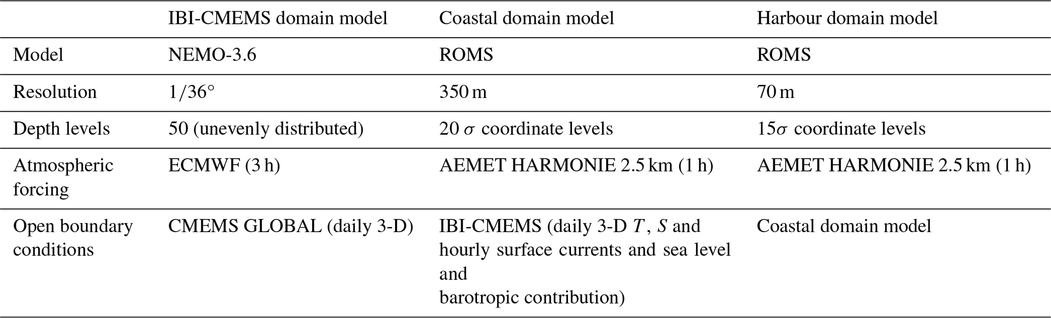
The harbour domain grid uses metocean forcing to downscale the coastal domain information to the more detailed resolution required. The nesting strategy was verified for inconsistencies with some continuity found between the IBI-CMEMS data and the SAMOA coastal application boundaries. The overall performance of SAMOA has also been successfully validated and was shown to capture major synoptic and mesoscale features mainly inherited from the IBI-CMEMS solution, together with specific local features (Sotillo et al., 2020). Further validation of the IBI and SAMOA systems was carried out using data from the extreme Storm Gloria event in January 2020, with both systems capturing the arrival of the storm with adequate accuracy (Sotillo et al., 2021). The hydrodynamic grid characteristics can be found in Table 1.

Table 1 Basic characteristics of the circulation numerical models used in the nested system (IBI and coastal and harbour domain models).

The wave component was obtained using the open-source Simulating Waves Nearshore (SWAN) model adapted to provide a wave height forecast downscaled to the Barcelona coastline using the nesting grid scheme and a resolution of $\mathrm{1}/\mathrm{20}$° (Allard et al., 2002). The SWAN-based system is formulated on the spectral reconstruction technique of sea states to compute random, short-crested wind-generated waves in coastal regions and inland waters. The wave data were also downloaded from the CMEMS server using the Download_data script.

2.3 Nested hydrodynamic grids

As mentioned previously, circulation data as numerical simulations available from PdE through the OPeNDAP server were provided in A grids, and although the IBI-CMEMS data were also in regular A grids, further configuration was necessary due to the coastal and harbour grids being oriented towards the coastline with some areas in these grids containing no data. To overcome this, an interpolation between the three grids that filled out empty values in the grids with higher resolution with the equivalent spatiotemporal data from the lower-resolution grids in these points was carried out using the UPC_resample_datasets script. The result of this interpolation can be seen in Fig. 2a. This script also produces and additional interpolation in the lower-resolution IBI-CMEMS grid due to the difference in temporal data, since CMEMS data are provided 30 min past the hour, and OPeNDAP data are provided on the hour, requiring previous and post-simulation temporal data to be downloaded in a process automated in the download script.

The u and v components of the hydrodynamic data of each grid were nested using the Parcels NestedField object in order of higher to lower spatial resolution, as shown in Fig. 1 (Delandmeter and Van Sebille, 2019). The nesting approach allowed the highest-resolution data to be used in the areas where it is available while utilising lower-resolution data elsewhere. The mean module intensity and current velocities in the nested grids (Fig. 2a), as well as the coastal and harbour grid boundaries (Fig. 2b and c respectively), are shown for a specified date. To use nested grids in the simulation, the nested_domain variable in the configuration file must be set, otherwise it defaults to the lowest-resolution grid. Artificial stagnation of particles on the coastline, which can be a concern when using A grids, was circumvented by deleting the particles on crossing a predetermined land–water boundary as described in Sect. 2.6.

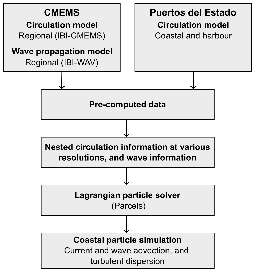
Figure 1 Schematic representation of the coupled plastic dispersion model components.

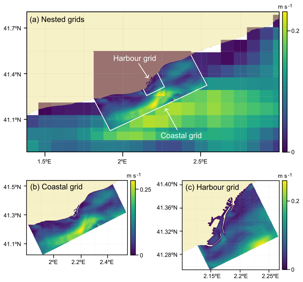
Figure 2 Example of hydrodynamic grids displaying module intensity and current velocity (m s⁻¹) for 23 March 2017.

2.4 Lagrangian particle simulations

The particle dispersion submodel was adapted to work at a coastal scale using the described hydrodynamic information to produce particle trajectory computations of virtual particles. The transport processes included in the motion of the virtual particles are coastal currents, wave data in terms of the Stokes drift, turbulent diffusion due to subgrid-scale diffusion and beaching. Particle simulations are conducted using the UPC_main_simulation script, with the required functions stored in an objects file, UPC_parcels_objects. If the nested_domain variable is set, the get_nested_fieldset function in the objects file is assigned as a fieldset, a class that holds hydrodynamic data needed to execute particles, otherwise the lowest-resolution fieldset, get_regional_fieldset, applies. The setting of the directories for the hydrodynamic data required for each fieldset can be found in the configuration file. Wave data are also added into a fieldset using a set_Stokes function found in the objects file, which reads the u and v Stokes drift components from the CMEMS wave data.

The particle trajectory simulation starts from an input of particles given at an initial time instant, and the position of the particles is then tracked in time moved by the mentioned transport processes. The input of particles can be given by direct information of marine debris particles measured in the domain, but it can also be obtained indirectly by inferring information about the amount of debris coming from rivers or wastewater discharge points located within the computational domain (see Sect. 2.8). These data are included in the simulation file through a sampler variable, which in turn is set by a ParticleXLSSampler function in the objects file that reads a spreadsheet with river input data. These data assume a continuous hourly or daily release of particles from a predetermined number of points as set in the particle_frequency variable in the configuration file. The spreadsheet name(s) and release coordinates are also specified in the configuration file. If the particle_frequency variable is set to None, the ParticleXLSCreator function is used, which creates individual, one-time releases for which spatial coordinates must also be provided in the spreadsheet input data.

The fundamental concept behind Parcels and any Lagrangian analysis is to integrate the advection equation (van Sebille et al., 2018):

$$\begin{array}{}\text{(1)}& {\displaystyle \frac{\mathrm{d}\mathit{x}}{\mathrm{d}t}}=\mathit{u}(\mathit{x},t),\end{array}$$

where x is the three-dimensional position of a virtual plastic particle in space, t is the time and u(x,t) is the three-dimensional Eulerian flow velocity field. u(x,t) incorporates the net current velocity and the Stokes drift. By integrating both sides of the equation, it can be rewritten as a pathway equation:

$$\begin{array}{}\text{(2)}& \mathit{x}\left(t\right)=\mathit{x}\left(t_{\mathrm{0}}\right)+\underset{t_{\mathrm{0}}}{\overset{t}{\int }}\mathit{u}(\mathit{x},t)\mathrm{d}t,\end{array}$$

which highlights that the location of a plastic particle at time t depends both on the initial three-dimensional position of the particle x(t₀) and the velocity field u(x,t). The pathway Eq. (2) by itself gives a trajectory of completely passive tracers. Note that u(x,t) is by definition a mean current and does not account for particle dispersion induced by diffusivity at smaller temporal scales.

2.5 Plastic particle dispersion

In Eq. (1) the velocity u(x,t) is by definition a mean velocity not incorporating subgrid-scale dispersion processes that are often parameterised as a diffusive process. In Lagrangian particle simulations, diffusive processes can be modelled as a stochastic, random displacement of particle positions as a function of the local eddy diffusivity (van Sebille et al., 2018). Whereas the time evolution of a trajectory advected by the mean current is accurately solved using an ordinary differential equation (ODE), which in the Parcels model is numerically solved using a fourth-order Runge–Kutta scheme, the time evolution of a stochastic process is solved using a stochastic differential equation (SDE). The SDE for a particle trajectory including diffusion is

$$\begin{array}{}\text{(3)}& \begin{array}{rl}\mathrm{d}\mathit{x}\left(t\right)& =\left(\mathit{u}\right(\mathit{x},t)+K(\mathit{x},t\left)\right)\mathrm{d}t+V(\mathit{x},t)\mathrm{d}W(\mathit{x},t)\\ \mathit{x}\left(t_{\mathrm{0}}\right)& ={\mathit{x}}_{\mathrm{0}},\end{array}\end{array}$$

where x is the particle position vector (x₀ being the initial position); u the velocity vector; K is the diffusivity tensor, where $K=\frac{\mathrm{1}}{\mathrm{2}}V{V}^T$; and dW(t) is a Wiener increment. The diffusivity tensor is a three-dimensional tensor incorporating the ocean–coastal diffusivity in the three-dimensional space. In Parcels, however, only horizontal diffusivity vectors can be simulated. These can be obtained from experimental data from the numerically simulated Eulerian eddy diffusivity (Bezerra et al., 1997). Three-dimensional eddy diffusivity can be obtained from ROMS simulations as a parameterisation of the subgrid diffusive processes in accordance with hydrodynamic forcing (wind, density, waves). However, pre-computed data available in the OPeNDAP do not incorporate such information, and a constant diffusivity parameter is generally used instead (OPeNDAP, 2022). When the horizontal diffusion coefficient (K) is constant, and time–space are invariant, the expressions in Eq. (3) can be simplified and integrated as

$$\begin{array}{}\text{(4)}& \mathit{x}\left(t\right)=\mathit{x}\left(t_{\mathrm{0}}\right)+\underset{t_{\mathrm{0}}}{\overset{t}{\int }}\mathit{u}(\mathit{x},t)\mathrm{d}t+R\sqrt{{\displaystyle \frac{\mathrm{2}\mathrm{d}tK}{r}}},\end{array}$$

where R is a random process representing subgrid motion with a zero mean and variance $r=\frac{\mathrm{1}}{\mathrm{3}}$ (Ross and Sharples, 2004). The hydrodynamic data input assumes current velocity data and Stokes drift data from the wave propagation model. A diffusion parameter, K_h, was added to the model as a constant field for the zonal and meridional components, using a spherical mesh. For all simulations described herein, the K_h value was set to 10 m² s⁻¹ (Okubo, 1971). This value has also been used in other studies using similar coarse horizontal resolutions, although preliminary simulations showed no material differences in terms of particle trajectory, destination or residence times with K_h values above 5 m² s⁻¹.

2.6 Plastic particle behaviours

Parcels allows the creation and use of specific kernels, which are small snippets of code that define particle dynamics and run during the execution of the simulation, depending on the requirements of the simulation (Delandmeter and Van Sebille, 2019). Particle behaviours can be declared as variables within the PlasticParticle class in the simulation file and can then be associated with a kernel in the UPC_Parcels_kernels file, resulting in the output of these data values from the simulation for further analysis. Examples of PlasticParticle variables used in kernels are particle residence time (age), trajectory length (distance_trajectory), real-time distance to the shore (distance_shore), and particle beaching (beached). The beaching definitions described in Sect. 2.9 used the beached variable and different kernels for different particle dynamics. When particles became beached or were exported from the study domain, they were deleted from the simulation using Parcels' core DeleteParticle behaviour.

2.7 Lagrangian model validation

To conduct a Lagrangian validation of the LOCATE model and evaluate its accuracy in predicting trajectories in coastal regions, comparisons were made between real and simulated trajectories. Drifter data were used from the Mobile Autonomous Oceanographic Systems (MAOS) Argo Italy database, available from the National Institute of Oceanography and Applied Geophysics website (OGS, 2023). Drifter data were selected on the condition of having drogues <1 m to assess only the influence of surface currents, including the Stokes drift, as it was assumed more realistic for a floating particle. Drifters that had trajectories that crossed the study domain were selected from the database, with priority given to drifters with data where the high-resolution hydrodynamic grids applied and those that were deployed from 2017 for which these data were available. Validation simulations were conducted for the available drifters. CODE drifter 6592, deployed in February 2022 was chosen as the most suitable because its trajectory crossed the coastal and harbour grids for a period long enough to analyse the skill of the model to forecast the trajectory 6, 24 or 72 h ahead, compared as a function of when the forecast started. CODE drifters 6607 and 6608 only crossed the coastal domain and were released within a minute of each other in March 2022.

For drifter 6592, simulations were conducted from the point where the trajectory transected the coastal grid boundary, at coordinates 41.18162° N, 2.24084° E. The provided data did not include timestamps, only a deployed and end date. It was assumed, however, that the drifter was fully operational and recording data at regular intervals, thus a reconstructed trajectory using the coordinates and the number of data points available were linearly interpolated to provide hourly data points, from which 100 particles were released at every step. Particles were released in the period 9 March 18:11:00 to 14 March 2022 18:11:00 LT (GMT + 1). The number of particles was determined through a sensitivity analysis of the standard deviation using varying amounts of particles (Castro-Rosero et al., 2023). Simulations for drifter 6607 were conducted at coordinates 41.19657° N, 2.27386° E from the period 11 March 09:14:00 to 14 March 2022 22:14:00LT (GMT + 1) and for drifter 6608 from coordinates 41.20218° N, 2.28279° E from the period 12 March 07:13:00 to 15 March 2022 09:13:00LT (GMT + 1). The same simulations were conducted using only the IBI-CMEMS grid, and with nested grids.

The comparison of the simulated versus the observed trajectories was based on the normalised cumulative Lagrangian separation (NCLS) distance skill score (SS) tests developed by Liu and Weisberg (2011). NCLS is defined as the cumulative sum of the separation distance between the observed and simulated trajectories (D) weighted by the length of the cumulative observed trajectory length (L):

$$\begin{array}{}\text{(5)}& \text{NCLS}={\displaystyle \frac{D}{L}}={\displaystyle \frac{{\sum }_{i=\mathrm{1}}^N{d}_i}{{\sum }_{i=\mathrm{1}}^N{\text{lo}}_i}},\end{array}$$

where N is the total number of time steps, d_i is the separation distance between the simulated and observed endpoints at time step i, and lo_i is the length of the observed trajectory. A reduced NCLS value implies an improvement in model performance, with a value of 0 implying a perfect fit between the simulated and observed values. The SS was calculated from the cumulative d and lo values for all time steps using a non-dimensional tolerance threshold (n) corresponding to the no-skill criterion of the simulated trajectory. In the same way as the present work, the value of this threshold is generally set to 1 (Liu and Weisberg, 2011; Révelard et al., 2021). The SS is defined as

$$\begin{array}{}\text{(6)}& \text{SS}=\left\{\begin{array}{ll}\mathrm{1}-{\displaystyle \frac{\text{NCLS}}{n}},& (\text{NCLS}\le n)\\ \mathrm{0},& (\text{NCLS}>n).\end{array}\right.\end{array}$$

Using the established threshold value, a SS value of 1 implies exact matches between simulated and observed trajectories. Distances were calculated using the geopy.distance Python module using the WGS-84 ellipsoid (Geopy, 2022). As part of the default particle behaviour in the model, particles that moved out of the study domain boundary (i.e. were exported) or became beached were detected, recorded and subsequently deleted from the domain for computational efficiency purposes. To maintain statistical rigour for the validation analysis, particles were not deleted when they became beached or were exported. Therefore, the same number of particles that were released was used in the validation calculations, with the last available coordinates registered either on the perimeter of the study domain or on the coastline used to calculate cumulative distances and the SS for subsequent time steps.

2.8 Plastic particle data inputs and release points

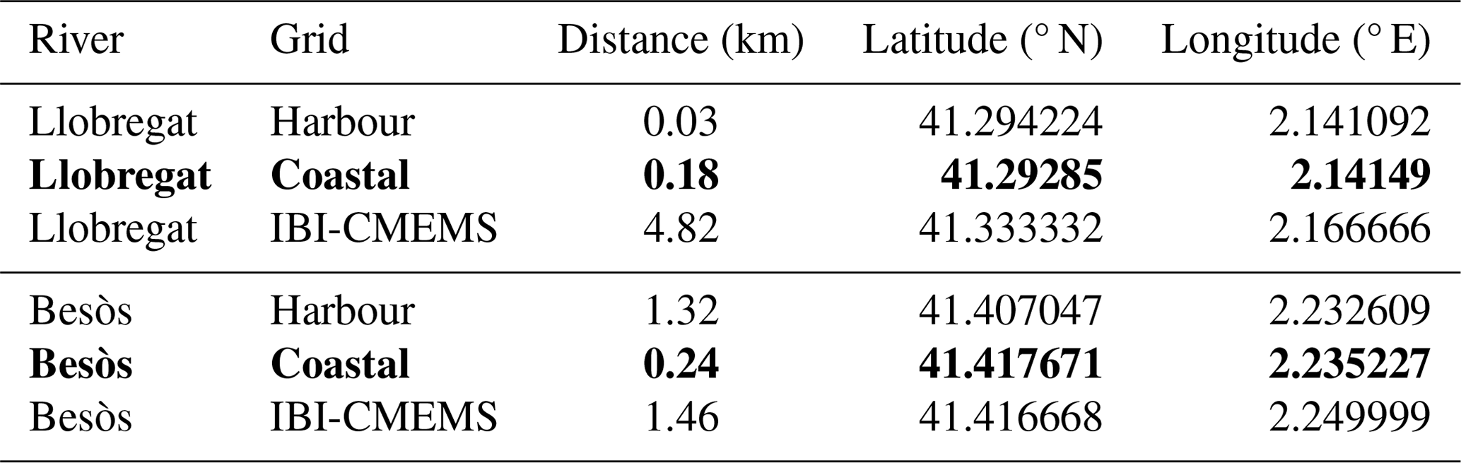
The high amounts of coastal marine debris and high flux rates observed in the study area allowed for the testing of beaching definitions and the applicability of those used in larger-scale studies to smaller coastal settings. Two Lagrangian simulations were conducted using the same input data: one using nested hydrodynamic grids and the other using a low-resolution IBI-CMEMS grid to compare particle beaching, residence times and trajectory distance. Particle release coordinates were selected based on the most proximal nodes from the coastal grid to each river mouth midpoint since it provided the highest resolution covering both river mouths. The release point for the Llobregat River (41.294468° N, 2.140995° E) was approximately 180 m distance from the river mouth midpoint, and that of the Besòs River (41.418909° N, 2.232839° E) was approximately 240 m from the river mouth midpoint. The selected coordinates for the particle release points are highlighted in bold in Table 2. The separation distance of both points was within the spatial resolution of the coastal grid.

Table 2 Closest nodes from each domain to the river mouth midpoint coordinates showing respective distances. The selected nodes are shown in bold.

The coastline in the study domain was divided into 16 different zones as shown in Fig. 3, which also shows the coastal and harbour grid boundaries. Demarcated zones were based on current official municipal demarcations according to the Área Metropolitana de Barcelona (AMB) or prominent features, such as port areas or beaches.

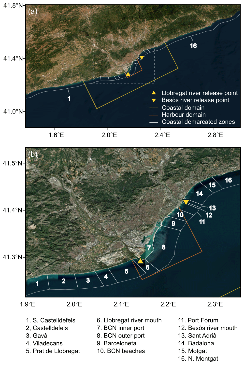
Figure 3 Demarcation of zones on the coastline (numbered) within the study domain area (a), with the dashed rectangle representing a closeup of the city area (b). Data source for (a) and (b) is ESRI.

The simulation period was limited to 261 d spanning 1 February to 19 October 2017 due to constraints in the availability of high-resolution hydrodynamic data before February 2017. The input component x(t₀) consisted of observational data of debris outflow from the Llobregat River and Besòs River around the city of Barcelona sourced from Schirinzi et al. (2020). As the river debris outflow data were irregular in time, a linear interpolation was applied to reflect realistic conditions of continuous debris release throughout the simulation period as illustrated in Appendix A. A total of 552 480 particles were simulated throughout the simulation period, with particles released every hour based on the interpolated daily amounts from each release point.

2.9 Particle beaching and beaching sensitivity analysis

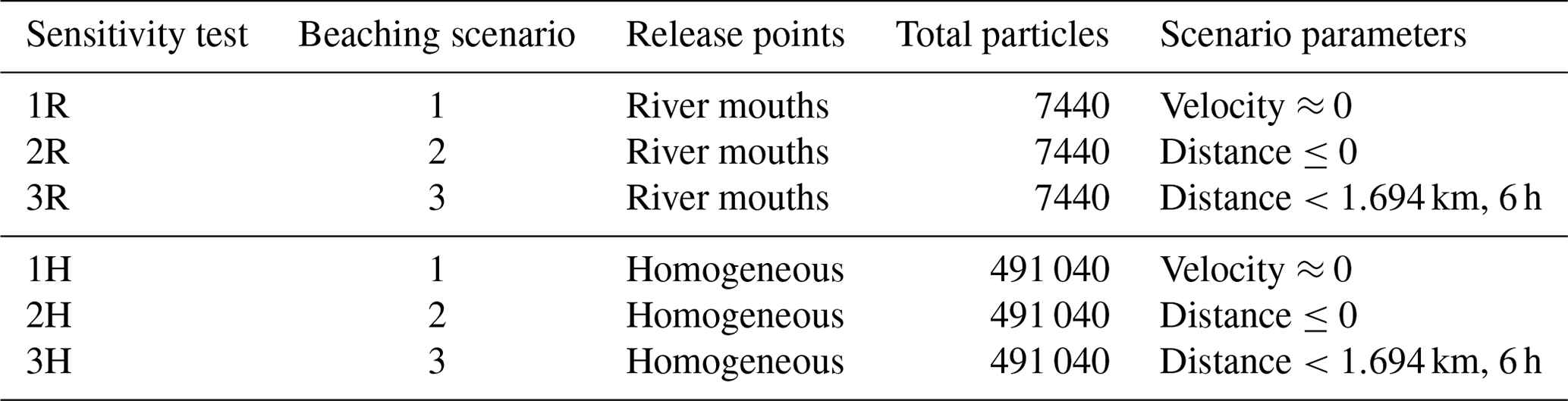
A beaching module was developed to parameterise particles that crossed the land–water boundary using the variables specified in Sect. 2.6 and the kernels listed below. A beaching sensitivity analysis was carried out in two parts with three different scenarios:

• a.

  using the two release points of river outflow from the Llobregat and Besòs rivers as per the simulations that compared the use of the IBI-CMEMS grid and nested grids (Table 2)

• b.

  releasing particles homogeneously in the study domain as a control using the coordinates of 132 nodes on the IBI-CMEMS domain that were on water (Appendix C).

In scenario 1 a particle was considered beached when u and v velocities were effectively stationary ($\le \mathrm{1}\times {\mathrm{10}}^{-\mathrm{16}}$ m s⁻¹), using the beaching_velocity kernel. In scenario 2 a particle was considered beached when it physically crossed the land–water boundary determined by a distance-to-shore parameter ≤0 m with pre-calculated distances from high-resolution shoreline data, using the beaching_distance kernel. In scenario 3, a time dependency was introduced linked to a distance parameter from the shoreline derived from the daily mean current velocity of 0.078 m s⁻¹ during the study period, as depicted in Fig. 4. Given the proximity to the shoreline of the particle release points, a time frame of 6 h was used resulting in a distance condition of 1.694 km. The latter scenario used the beaching_proximity kernel.

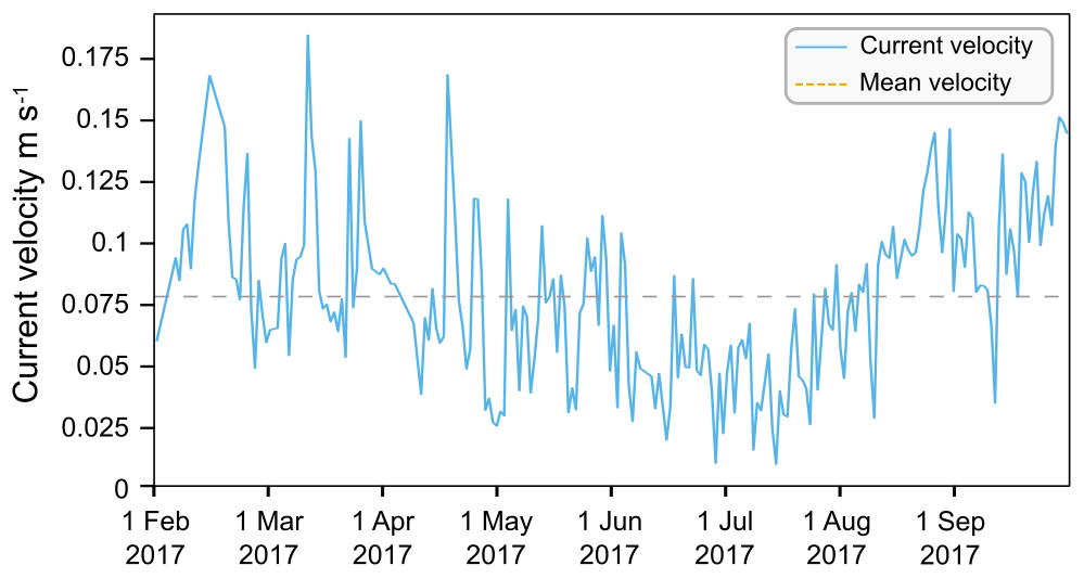
Figure 4 Mean daily current velocity of the IBI-CMEMS grid for the period 1 February to 30 September 2017, with the mean velocity for the period.

Given that kernels in Parcels are limited to basic arithmetic operations and conditions, Parcel's interpolation capabilities were utilised to calculate the real-time minimum distance between particle and shoreline for scenarios 2 and 3 with distance data available in a fieldset so that particles could effectively detect the shoreline given a beaching parameter. This was achieved by incorporating the distance-to-shore data into grids with the same structure as the hydrodynamic data. Information on the Catalan coastline was obtained as a linestring in a shapefile format with 259 080 data points, excluding islands or islets, using UTM-31N with datum ETRS89 as the cartographic reference system using a scale of 1:50 000 (ICGC, 2020). The linestring was edited in the open-source QGIS software to only include data within the boundaries of the study domain. Node coordinates of the hydrodynamic grids were differentiated and classified as being on land or at sea, and the minimum distance between all the node coordinates and the shoreline data was calculated using the geopy.distance Python module (Geopy, 2022). For land nodes, distances were assigned negative values to ensure correct interpolation when crossing the land–water boundary. Distance data for each node to the shoreline in each domain were added as netCDF4 files in the simulations, enabling the nesting of these files in the same manner as the nested hydrodynamic grids. The preprocessing required to prepare the distance grids is included in a series of Python scripts in the scripts folder.

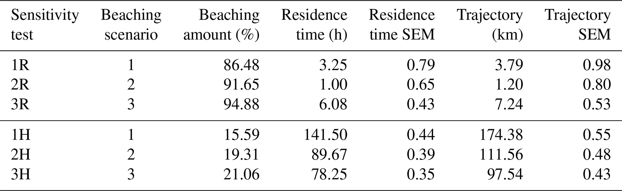
A total of five particles were released every hour from each point for the period 1 March 00:00:00 to 31 March 2017 23:00:00, with a total of 3720 particles released from each point. In the first part of the sensitivity analysis with the two river release points, a combined total of 7440 particles were released in the domain. In the second part, where particles were released homogeneously there were a total of 491 040 particles released from 132 points (Table 3).

Table 3 Parameters, release points and total particles released for beaching sensitivity tests.

3 Results

In this section, the main numerical experiments that were conducted are presented. Firstly, the validation results of the LOCATE model are provided, followed by a comprehensive beaching sensitivity test using different criteria to define beaching parameters. Finally, beaching amounts and residence times of simulations using the same debris outflow data are compared using nested grids and the IBI-CMEMS grid.

3.1 Lagrangian validation of LOCATE

The model validation process involved conducting simulations along the trajectory of the drifter data to qualitatively and quantitatively compare the observed (L) and the simulated (D) trajectory distance and SS calculations using different prediction horizons as illustrated in Fig. 5. The simulation times had decreasing forecast horizons of 1 h with every time step along the observed trajectory, with all simulations having the same end time. As seen in Fig. 5a, results from the progression of the SS values at different forecast horizons were nuanced when comparing simulations conducted with nested grids and the IBI-CMEMS grid. For a 6 h forecast horizon, there were two notable peaks of SS values, the first one at 13 h (IBI-CMEMS SS=0.41) and 15 h (nested grid SS=0.40) from the initial simulation and the second one at 43 h for both (IBI-CMEMS grid SS=0.43, nested grid SS=0.53). Results on a 24 h forecast horizon demonstrated a better performance for nested grids, with a peak at SS=0.49 at 13 h from the initial simulation, whereas the peak at 40 h was higher with the IBI-CMEMS simulation, SS=0.69 compared to SS=0.52 for the nested grid simulation. Overall, the 72 h forecast horizon was more stable with the nested grids with values exceeding 0.60 for simulations between 9 and 39 h from the initial simulation, with a peak of 0.68 for the simulation at 13 h. Simulations with IBI-CMEMS displayed much greater variability, with a peak of SS=0.80 at 36 to 39 h from the initial simulation. The IBI-CMEMS simulation had lower SS values than the nested grid simulations for the first 27 simulations (out of 48 total for each).

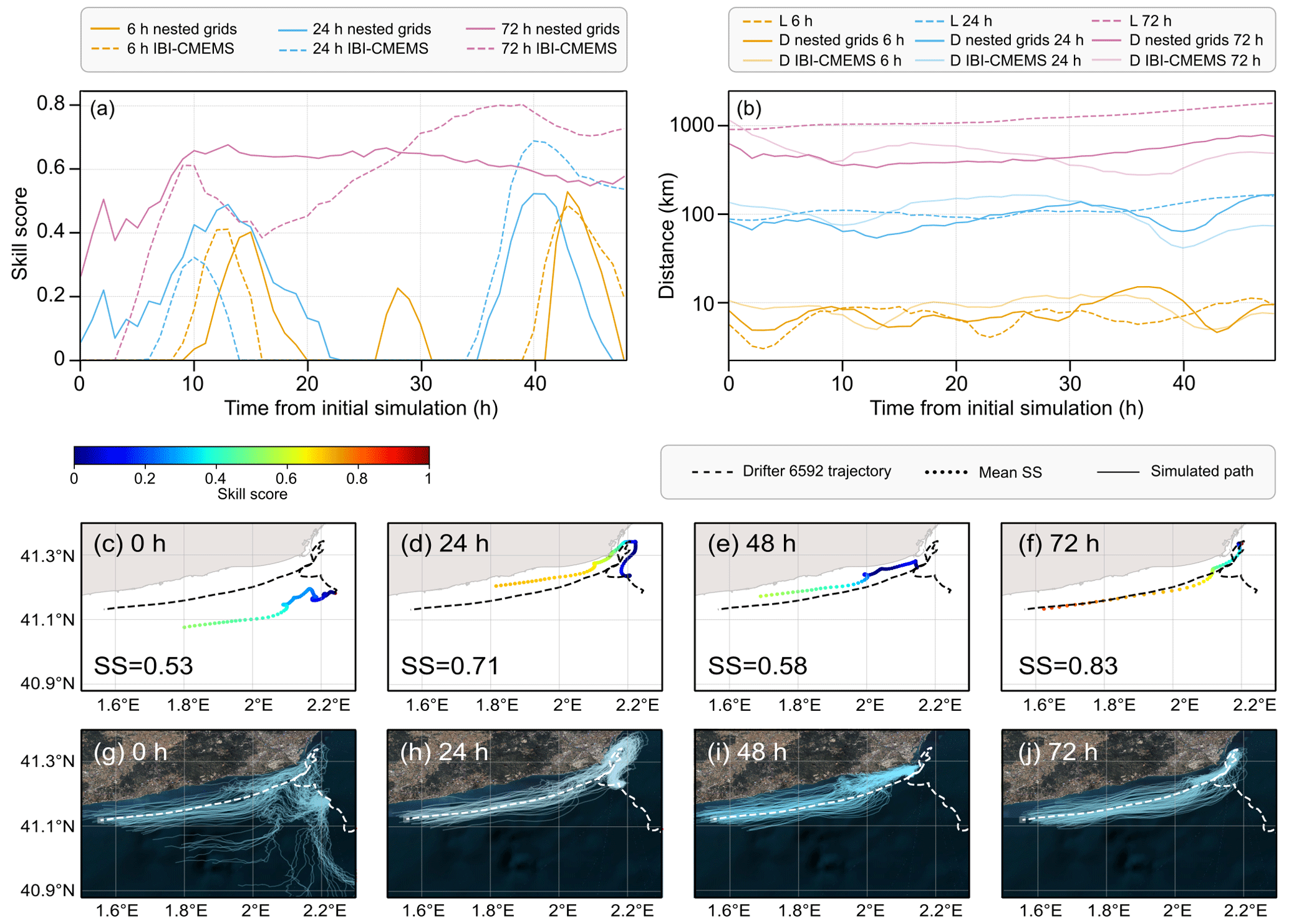
Figure 5 Lagrangian validation of LOCATE using data from drifter 6592 between 9 March and 14 March 2022 (maximum of 120 h) using the skill score test. Panel (a) illustrates the SS of the simulations at 6, 24 and 72 h forecast horizons using nested grids and the IBI-CMEMS grid. Panel (b) shows the time evolution of the cumulative distance (D) between the simulated and observed trajectories and the observed cumulative distance (L) for the same simulation using nested grids and the IBI-CMEMS grid at 6, 24 and 72 h forecast horizons using a logarithmic scale. Panels (c–f) show the SS of mean trajectories for simulations with nested grids at 24 h intervals with their final SS, with a SS colour band for scale. Panels (g–j) show the trajectories of the simulated particles using nested grids as well as the drifter trajectory for comparison. Data source for (g–j) is ESRI.

As illustrated in Fig. 5b, at a 72 h forecast horizon, the cumulative observed distance of the drifter (L) consistently exceeded the simulated cumulative distance (D) in both types of simulations, reaching a peak value of 1805 km for L. In comparison, the highest D values were 792 km for the nested simulations and 1264 km for the IBI-CMEMS simulation. Qualitatively, as depicted in Fig. 5b the simulations using nested grids demonstrate a similar growth pattern, whereas the IBI-CMEMS simulations displayed periods of cumulative distance increases and decreases. The SS of the mean trajectory of the initial simulation (Fig. 5c and g) reflected the variability of the simulated trajectories. Notably, some beaching was observed in Fig. 5i and j around the Barcelona city area, potentially indicative of the lower SS value in Fig. 5e at 48 h from the initial simulation. The SS value at 72 h was very high (SS=0.83), with increasing cohesiveness between the simulated and observed trajectories as the simulations progressed over the track of the drifter trajectory. It is important to note that these results were not observed in the SS forecast horizon plot (Fig. 5a) or the cumulative distance plot (Fig. 5b), as the 72 h forecast horizon was not available beyond the 48th simulation.

As seen in Fig. 6, the SS of drifter 6652 was much higher when using the nested grids than only the IBI-CMEMS grid (SS=0.53 compared to SS=0.07). For drifter 6607 the IBI-CMEMS grid performed slightly better (SS=0.74 compared with SS=0.68). Qualitatively, it can be observed that the particle trajectories using the IBI-CMEMS grid were being displaced towards the coastline with substantial beaching of particles, while the particle trajectories with the nested grids moved further out to sea, with the real drifter trajectories somewhat in the middle. The same difference in SS values was observed for drifter 6608 but with nested grids performing better with SS=0.61, and a similar particle displacement pattern as drifter 6607 can be observed.

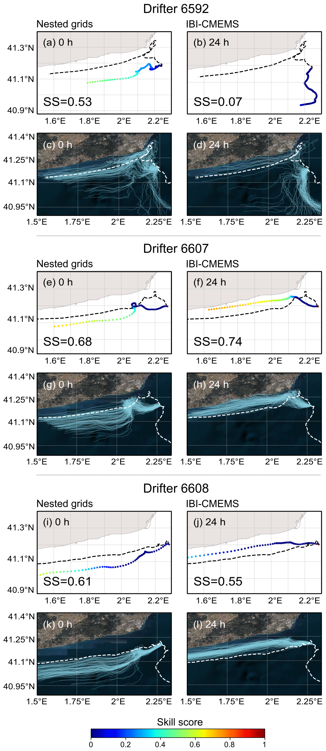
Figure 6 SS of the mean trajectories using nested grids and the IBI-CMEMS grid for drifter 6592 in panels (a) and (b), drifter 6607 in panels (e) and (f), and drifter 6608 in panels (i) and (j). Trajectories of the simulated particles for the simulations for drifter 6592 in panels (c) and (d), drifter 6607 in panels (g) and (h), and drifter 6608 in panels (k) and (l). Data source for panels (c), (d), (g), (h), (k), and (l) is ESRI.

3.2 Beaching sensitivity analysis

Figure 7 illustrates the distance from the shoreline at which particles become beached according to the different criteria for each scenario. As expected, tests with scenario 2 (2R and 2H) show particles closely aligning with the actual shoreline, while tests using scenario 1 follow the boundaries of the hydrodynamic grids of varying resolutions with current velocity data. The results presented in Table 4 indicate that the homogeneous particle release, serving as a control, yielded much lower beaching amounts (<21.06 %) compared to releases from the two river release points close to the shore (86.48 % to 94.88 %). The highest beaching amounts of each group were found in tests using scenario 3 (3R and 3H). The residence times for the tests using scenario 1 (1R and 1H) were notably longer than for tests using scenario 2. Additionally, trajectory distances were greater in scenario 3 when particles were released close to the shoreline, although this trend was reversed in the homogeneous particle release. The value of 6.08 h for test 3 includes the 6 h parameter for that scenario and the first time step thereafter, set to 5 min.

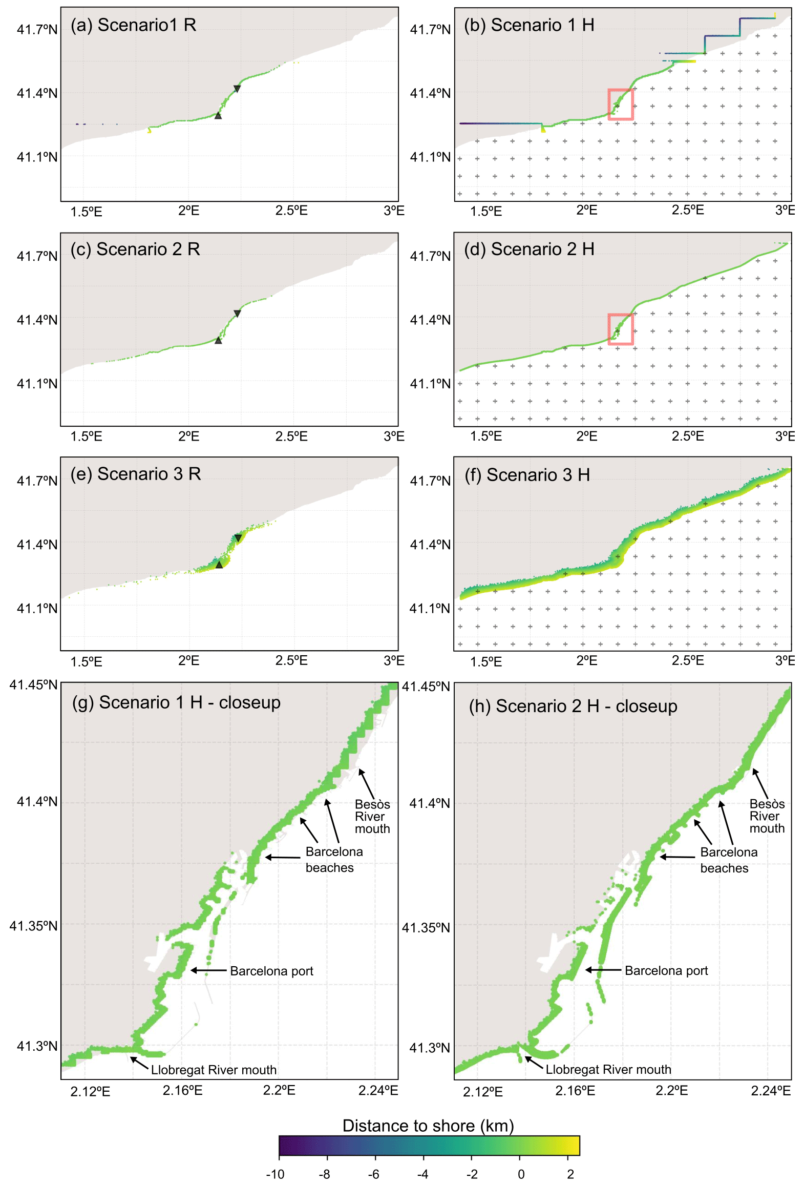
Figure 7 Locations of beached particles for beaching sensitivity tests. Markers represent particle release points, with a triangle up marker representing the Llobregat River, a triangle down marker representing the Besòs River and the plus marker representing nodes on the IBI-CMEMS domain for the homogeneous particle release tests. The red rectangle area in panels (b) and (d), representing the Barcelona port Barcelona beaches, the Llobregat River and Besòs River mouths, can be found in panels (g) and (h) respectively.

Table 4 Beaching amount percentage, median particle residence time and median particle trajectory with the standard error of the mean (SEM) for river release (R) and homogeneous release (H) tests for each scenario. Scenario 1 used current velocity to determine beaching, scenario 2 used a distance-to-shore parameter, and scenario 3 used a time condition with the distance-to-shore parameter.

The area depicted in Fig. 7g (scenario 1) and h (scenario 2) was covered by the high-resolution hydrodynamic grids, with the area approximately between latitudes 41.3 and 41.4° N and longitudes 2.14 and 2.22° E being covered by the harbour grid, and the rest by the coastal grid. Notable differences in the beaching patterns can be discerned due to the difference in how the coastline is resolved. In scenario 1, the beaching patterns where the coastal grid was applied appear jagged, although this was also the case at a smaller scale due to the higher resolution where the harbour grid was applied, especially around the Barcelona beaches. Additionally, small-scale structures, such as piers and groynes, are not considered. In contrast in scenario 2, the beaching patterns are in much tighter alignment with the real coastline, with port structures such as the jetties and other small-scale structures fully resolved.

3.3 Simulations of river release particles

The snapshots presented in Fig. 8 correspond to the simulation using nested grids and the distance-to-shore beaching parameter (scenario 2), providing a visual representation of how the model uses hydrodynamic data of varying resolutions. For illustrative purposes, the month of May 2017 was selected corresponding to the period of highest particle release from the Llobregat River, as shown in Fig. A1. The snapshots capture the dispersion of particles over 6 d intervals, starting from the beginning of the month. As the month progressed, the snapshots revealed the particles moving towards the coastline and dispersing along the majority of the coastal region within the domain. Some particle accumulation was observed towards the south of the domain on 31 May 2017 due to boundary conditions where the mean current velocity for that day was close to 0 m s⁻¹ in the nodes west of 1.6° E between 41.2 and 40.95° N. The particle density maps highlight the highest densities observed close to the release points, as evidenced on 7 May and 31 May 2017.

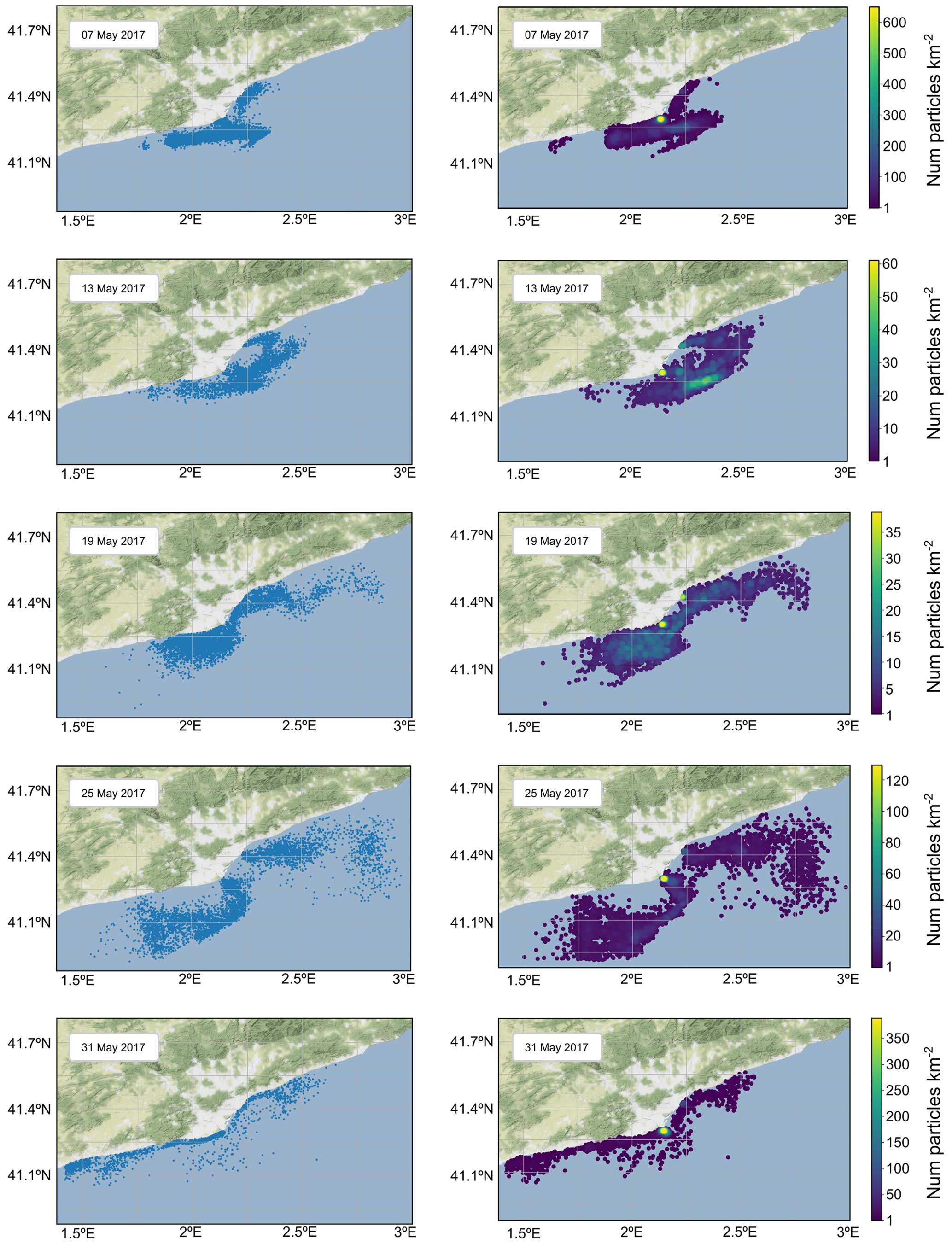
Figure 8 Simulation snapshots using nested grids for dates in May 2017 at 23:00 LT (GMT + 1). Maps on the left show the dispersion of particles released. Maps on the right show particle density of the number of particles per square kilometre (n km⁻²).

As can be inferred in Fig. 9, the total beaching amounts observed in the simulations with the IBI-CMEMS grid and nested grids using the distance-to-shore beaching parameter were very high. The nested grid simulation revealed a beaching proportion of 91.5 %, with 8.5 % of particles being exported, while the simulation employing the IBI-CMEMS grid exhibited a beaching proportion of 95.8 %, with 4.2 % of particles being exported. When examining the beached quantities within the demarcated zones in Fig. 9a, there were marked differences between both simulations. The Prat de Llobregat area received 12.7 % more beached particles with the IBI-CMEMS simulation (24.0 % with the IBI-CMEMS grid compared to 11.3 % with nested grids), whereas the Llobregat River mouth showed 8.7 % more beached particles with the nested grid simulation (43.5 % with nested grids compared to 34.8 % with the IBI-CMEMS grid).

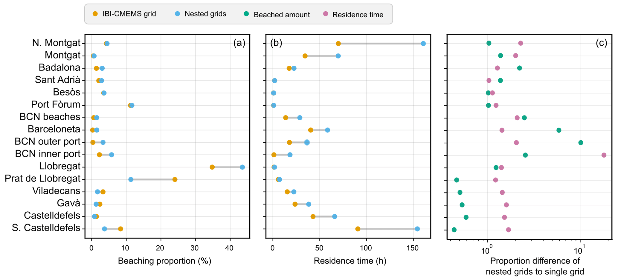
Figure 9 (a) Beaching amounts per demarcated zone as a percentage of the total amount of beached particles for the nested grids and IBI-CMEMS grid simulations. (b) Residence time median per demarcated zone for the nested grids and the IBI-CMEMS grid simulations. (c) Proportion difference of beaching amount and residence time between simulations using nested grids and the IBI-CMEMS grid on a logarithmic scale.

The larger beaching differences were found in regions of complex shoreline configuration. For instance, the amount of beaching was over 10 times higher in the external port area with the nested grid simulation and 2.5 times higher inside the port area. Barceloneta Beach experienced over 6 times as many beached particles with the nested grid simulations, and the other city beaches exhibited over 2.5 times as many beached particles. The number of beached particles in these areas, however, was lower than in other areas such as the Llobregat River mouth and surrounding areas. Residence times increased substantially as the zones moved further away from the release points, particularly evident in the areas south of Castelldefels and north of Montgat. The increase in residence times was also observed between release points where the higher-resolution grids provided the hydrodynamic data. Particle residence times consistently showed higher values for the simulation using the nested grids, with the inside of the port area registering values that were 18 times higher when compared to the same area in the IBI-CMEMS simulation.

4 Discussion

4.1 Numerical models and coastal processes

Numerical models of marine debris transport to date have been valuable in providing debris budget estimates, measuring fluxes and studying interconnectivity at oceanic scales (Chassignet et al., 2021; Eriksen et al., 2014; Law et al., 2010; Lebreton et al., 2012; Maximenko et al., 2012; Onink et al., 2019, 2021; van Sebille et al., 2012, 2015). Some studies have focused on semi-enclosed basins such as the Mediterranean Sea to establish debris dispersion and accumulation patterns (Kaandorp et al., 2020; Liubartseva et al., 2018; Mansui et al., 2015, 2020; Zambianchi et al., 2017). The models used in the aforementioned studies use similar coarse hydrodynamic resolutions, typically of ≥2.5 km. The application of Lagrangian models to nearshore systems with complicated geometries and at smaller scales is much less mature than oceanic-scale models. This is likely due to the complexities involved and the fact that the modelling of particle beaching in a shoreline defined by coarse resolutions can be difficult, leading to inconsistencies or inaccuracies (Critchell et al., 2015; Critchell and Lambrechts, 2016; Neumann et al., 2014; Yoon et al., 2010; Zhang, 2017). To address these limitations, nested hydrodynamic grids with varying resolutions can provide simulations with greater precision in high-interest areas such as harbours and adjacent coastal waters, where higher-resolution data may be available. Even if the high-resolution data do not encompass the entire study domain, large parts of the study domain can be covered. In the present study, the high-resolution coastal grid spanned all the demarcated areas to at least some extent as illustrated in Fig. 3.

The results from the Lagrangian validation of the model indicate that the similarity of the simulated trajectories to the real trajectory of the selected drifters using LOCATE was highly dependent on the resolution of the Eulerian hydrodynamic currents data. These results are consistent with a study by Castro-Rosero et al. (2023) in the Black Sea which also demonstrated the suitability of LOCATE for predicting the motion of floating marine debris. Furthermore, high skill stability and performance for the 72 h forecast horizon were observed when utilising nested grids, a commonly used threshold in other studies to determine the sensitivity of the SS test (Révelard et al., 2021). The comparison of simulations conducted using nested grids and the IBI-CMEMS grid across all forecast horizons presented somewhat mixed results. However, as seen in Fig. 5a, the SS values for the 72 h forecast horizon were higher for 56.25 % of the simulations conducted using nested grids. This is indicative of the challenges associated with predicting trajectories close to the shoreline influenced by coastal processes, amplified by the strong influence of the alongshore northern current as seen south of the Barcelona city area in Fig. 5g–j and in the trajectories in Fig. 6. There was a notable difference in how the different grids performed during the dates of the simulation, with the IBI-CMEMS grid showing the northern current much closer to the coastline than the higher-resolution grids, with a greater probability for beaching as seen for drifter 6607 in Fig. 6h. The consistent and generally higher SS values of the simulated drifter trajectories when using the nested grids compared to more variable results when using the IBI-CMEMS grid demonstrate that using higher-resolution data in nested grids can produce generally more favourable results. Drawing direct comparisons between nested grids and the IBI-CMEMS grid using the SS test, however, is challenging. Within a single trajectory, the influence and contribution of each grid as a particle moves across different domains cannot be isolated due to the cumulative nature of the test, even if it is possible to numerically determine which grid has provided the hydrodynamic data for that time step. Additionally, an area of future work could address the paucity of available and suitable drifter information at coastal scales where high-resolution hydrodynamic data may apply.

In the simulation comparison between nested grids and the IBI-CMEMS grid, the particle release coordinates coincided with coastal nodes close to the midpoint of the Llobregat and Besòs River mouths to prevent excessive accumulation of particles at the river mouths from a possible lack of hydrodynamic data at those specific points. While the coastal grid data included river contributions in the form of climatological run-off values and a constant salinity field, the actual outflow rates at the river mouths (mean values of 20.77 m³ s⁻¹ for the Llobregat River, and 4.33 m³ s⁻¹ for the Besòs River) were not included. Indeed, the real-time inclusion of discharge observations or inputs from hydrological forecast models is currently undergoing development in the SAMOA system. Once implemented, this enhancement would allow forcing to an extended run-off rate at every coastal grid point, thereby increasing the accuracy of simulations in areas adjacent to the river mouths where very high beaching rates can be found (Sotillo et al., 2020).

Numerical models that only rely on low-resolution hydrodynamic grids have been shown to inadequately reproduce submesoscale structures, particularly evident in the western Mediterranean region, causing model underperformance and potential problems when tracking maritime emergencies (Sotillo et al., 2021). Notably, particle residence times were substantially higher in areas of topographic complexity when using nested grids, such as the inner port area displaying 18 times higher residence times as depicted in Fig. 9c, which is consistent with findings reported by Sotillo et al. (2021), suggesting that some coastal processes were incorporated in the simulations with nested grids. There were elevated residence times and beaching amounts in all other areas covered by the harbour grid where other complex coastal structures could be found, such as beaches, groynes and piers. Higher residence times were also observed in other areas, particularly those close to the study domain limits, likely due to prolonged residence times of particles when traversing the higher-resolution domains during the simulation.

The differences in beaching amounts between grids display variability in some areas as illustrated in Fig. 9a. For instance, the Llobregat River mouth showed 8.7 % more beaching when using nested grids (43.5 % compared to 34.8 %). In contrast, the Prat de Llobregat, an adjacent area to the south of the Llobregat River mouth, experienced over twice the amount of beaching (24.0 % compared to 11.3 %) when only using the IBI-CMEMS grid. This observation suggests that the IBI-CMEMS grid may have higher current velocities around the Llobregat River mouth than the higher-resolution grids, leading to the transport of more particles to the neighbouring area to the south.

By incorporating high-resolution data and utilising a detailed coastline to parameterise particle beaching, it is possible to distinguish complex structures in regions with high fractal dimensionality and natural barriers. In contrast, using lower spatial resolutions may lead to an underestimation of beaching amounts in areas containing complex structures or adjacent to them. The external port area, which is separated by a barrier from the internal port area, exhibited markedly higher beaching amounts when high-resolution grids were applied. Thus, a distinctive feature of the Barcelona harbour, which has two mouths separated by a quay increasing the complexity of the hydrodynamic behaviour of the port, was considered when applying the harbour grid (Sotillo et al., 2021). Solely relying on low-resolution grids such as the IBI-CMEMS grid for dispersion tracking or even as a land detection mechanism using current velocity for particle beaching, as seen in some larger-scale studies, is observed to be insufficient or even imprecise for coastal-scale simulations. Some limitations do exist, however, in the high-resolution hydrodynamic data utilised in this study.

The hydrodynamic data used in this study did not include wave-induced Eulerian (mean) currents, therefore omitting some important coastal processes such as longshore currents that can be very important in the transport, deposition and redeposition of material in areas potentially far away from the point of emission. Despite the highest-resolution grid used resolving down to 70 m, it remains insufficient to resolve undertow or rip currents and resulting gyres that not only shape sandy shorelines but also contribute to the transport of material offshore especially where convergence occurs by longshore currents (Hinata and Kataoka, 2016). Currently, the wave component of the hydrodynamic data is a one-way coupled system between the regional CMEMS physical model (IBI-PHY) and the IBI wave products (IBI-WAV) that includes the Stokes drift, wave-induced mixing and wind drag coefficient formulas based on sea states. These wave data, however, are not included in the hydrodynamic data provided by the SAMOA application, although efforts are being made to incorporate them (García-León et al., 2022). Indeed, a positive impact has been observed in model predictions from coupling wave-current data in open water and shallower coastal areas, especially during extreme weather events such as Storm Gloria in January 2020 (Sotillo et al., 2021). In this study, the Stokes drift component was provided by the IBI-WAV system, which has an even lower resolution ($\mathrm{1}/\mathrm{20}$°) than the IBI-CMEMS grid ($\mathrm{1}/\mathrm{36}$°) and was not integrated into the nested solution (CMEMS, 2023).

The use of LOCATE to perform Lagrangian simulations using nested hydrodynamic grids is not limited to the current study domain and could be adapted and transposed to other areas where hydrodynamic data in varying resolutions may be available. Numerical simulations of other coastal regions in Spain are hosted on the PdE website, making the extension of the developed system to other locales relatively simple (García-León et al., 2022; Sotillo et al., 2015, 2021). Hydrodynamic grids may require some adaptation to work with each other even if they have the same regular A grid configurations to ensure compatibility between grid structure, orientation and time data, although the scripts provided in LOCATE address these issues. It is important to note that LOCATE can also be configured to be used with C grids. While the nested grid functionality is featured in Parcels, LOCATE is specifically tailored to be used in coastal areas or localised studies. Parcels alone lacks the necessary considerations and requirements to provide precise simulations of marine debris at coastal scales, which are included in LOCATE and would require significant time investment and programming from scratch. LOCATE also includes important features required for more precise representations of particle beaching at such scales which could be relevant in beach debris management and can be easily configured to be used for a one-off particle release or a continuous debris discharge.

Another aspect that may require further refinement is the parameterisation of the horizontal diffusion coefficient. In similar studies, the K_h value was commonly set to 10 m² s⁻¹ where the hydrodynamic resolution applied was similar to that of the coarse-resolution data used in the present work (Okubo, 1971; Onink et al., 2021, 2022). The simulated dispersion process largely depends on the size of the mesh, the resolution used and the velocities therein; however, there is no experimental or empirical data to know what the appropriate K_h value should be used at the scales used in this study. A prudent approach was therefore taken to use the same K_h value throughout for consistency while recognising this is an area for future research. Nevertheless, the validation work using drifter data in the areas where the high-resolution hydrodynamic data were applied yielded good skill score values, as seen in Fig. 6.

Currently, plastic dispersion simulations assume that the driving force behind the movement of plastic particles is a linear combination of the Stokes drift and mean currents. While this approach is realistic in middle–low energetic conditions and in coastal regions relatively far from the coastline (100 m from the coastline to the continental shelf), it fails to account for wave-induced currents and processes that are not resolved by current models, having important implications regarding the movement and transport of material. Moreover, the spatial resolution constraints result in particles moving linearly towards land without being caught up in the surf and swash areas, potentially leading to underestimations of residency times (Hinata et al., 2017).

Another drawback of not including wave processes is that particle resuspension and subsequent redeposition events cannot be effectively parameterised in a deterministic manner given the scarcity of data to form the basis of probabilistic definitions. To address these limitations, a beach domain based on the Coupled-Ocean-Atmosphere-Wave-Sediment Transport Modelling System (COAWST), a numerical model with a resolution of 23 m, is being developed at the Universitat Politècnica de Catalunya. This grid will be nested into the harbour domain enabling very detailed simulations that can accurately characterise coastal processes. Wave–current interaction processes will be relevant in this domain as the transport of plastic particles in coastal environments is largely influenced by wave-induced motions, with waves in coastal regions being highly nonlinear as a consequence of wave-topography interaction.

4.2 Particle beaching

The effect of wind on the currents was incorporated into the coastal and harbour grids which have atmospheric forcing by AEMET and can have a significant influence on beaching amounts, with small changes even in the short term having important effects on the trajectories and accumulation patterns (Critchell et al., 2015; Rosas et al., 2021). Wind drag on particles, however, was not considered since it would require particle size, shape and buoyancy to be determined for virtual particles which are assumed to be floating just beneath the surface. The high beaching values in the simulations with the nested grids and IBI-CMEMS grid were higher than other recent studies which are dependent on region, scale and simulation period. As can be seen in Appendix B, the beaching amounts were highly variable, with some studies from the central and eastern Mediterranean Sea such as Politikos et al. (2017, 2020) recording meager beaching rates, while other studies such as Macias et al. (2019) observed amounts higher than the present study. Other prominent studies at oceanic scales such as Onink et al. (2021) and Lebreton et al. (2019) recorded lower beaching amounts than this study, with 77 % and 67 %, respectively, over integration times that span up to 20 years. Unfortunately, there is not enough comparable beaching data from other comparable numerical modelling studies at similar coastal scales as of yet.

Defining the parameterisation and inclusion of particle beaching in numerical models is crucial for identifying areas within the coastal zone that may experience increased pressure from plastic pollution, and the range of these different types of definitions can be seen in Appendix B. It is important to note that definitions used in larger-scale studies may not be suitable for localised analyses. Deterministic parameterisations, which are simpler in formulation than probabilistic parameterisations, often depend on whether a particle crosses the land–water boundary using current velocity, such as Lebreton et al. (2012), Macias et al. (2019, 2022), Politikos et al. (2017, 2020), Rosas et al. (2021) and Ruiz et al. (2022), and were represented under scenario 1. Another common deterministic parameterisation involves a predetermined distance travelled over a certain amount of time to indicate particle stagnation, such as Chassignet et al. (2021), Lebreton et al. (2019) and Mansui et al. (2015), and were represented under scenario 3. The beaching pattern in Fig. 7b under scenario 1 showed that there were no areas around the coastline that were left uncovered by data, and that beaching always occurred on land. Even if some cells around the coastline did not have velocity data, as seen in Fig. 2a, Parcels' interpolation capabilities use the zero velocity values from adjacent land cells to interpolate velocities of shoreline cells without velocity data. In this scenario, shoreline identification had different resolutions along the coastline, resulting in an overestimation of residency times and trajectory distances with respect to using a physical land–water boundary such as under scenario 2. While higher-resolution grids using current velocity in scenario 1 can adequately resolve areas like the inner port, the lower-resolution grids caused uncertainty, with particles potentially travelling several kilometres inland before being considered beached. This uncertainty hinders the determination of areas most at risk of receiving and accumulating marine debris, especially in areas which are only covered by the low-resolution data. While this may not be an issue in larger-scale studies, at coastal scales it may prevent correct identification of accumulation areas. Furthermore, scenario 3, which utilised a time and distance requirement, introduced additional uncertainty regarding the likelihood of beaching occurrence, with higher residence times and trajectory distances also observed. Additionally, particles drifting alongshore within the specified distance would be immediately considered beached after the specified time, effectively disregarding hydrodynamic conditions or data that may resolve coastal processes (if these are included) within the distance parameter, which could explain the higher beaching values observed. Conversely under this scenario, if a particle reaches a land cell where there is no velocity data before the time limit, it would continue to move due to the horizontal diffusivity that continues the stochastic movement of a particle, resulting in possible overestimations of residence times.

A distinct approach to particle beaching was provided in scenario 2 which introduced a deterministic beaching model that relied on a physical shoreline and pre-calculated distance data of nodes to the shoreline in a grid(s) used in a fieldset. This methodology enabled the calculation of distances between particles and the shoreline during the simulation to determine when and where they cross the land–water boundary, becoming beached if the distance to the shore is ≤0 as illustrated in the beaching sensitivity analysis (Fig. 7c and d). The main purpose of this beaching parameterisation is not to predict that beaching occurs on the real shoreline but to provide a consistent coastline independently of the hydrodynamic resolution used when nesting grids. Additionally, the interpolation and grid nesting capabilities of Parcels allowed distance calculations not to be limited by a decrease in spatial resolution throughout the domain. Although small-scale structures are seemingly resolved using this parameterisation, allowing for quantification of beaching at specific locations with much less difficulty than other scenarios, it is not consistent with the hydrodynamic coastline. Therefore the flow around the subgrid scale features resolved may not be based on physical processes, and the localised effects these structures could have on the hydrodynamic data are not considered. Additionally, the potential for the introduction of artefacts from artificial convergence cannot be ruled out in areas where the hydrodynamic coastline and the real coastline based on high-resolution shoreline data converge (see Appendix D). Whether these inconsistencies have material effects on the prediction of beaching patterns remains an area for future work. Other limitations of this scenario include the dependency on the availability of high-resolution spatial data and the requirement of preprocessing steps. In the absence of hydrodynamic data of such a fine resolution that may counter these shortfalls, this beaching parameterisation can provide a suitable compromise for small-scale studies and could lead to the development of further parameterisations at beach level in future research. It is crucial to underscore that the considerations for using a distance-to-shore beaching parameterisation are especially relevant for small-scale or localised studies where stakeholders may prioritise identifying specific at-risk areas. In contrast, concerns at a larger scale may differ significantly, and the parameterisations used in scenario 2 may not be as useful or meaningful then.

5 Conclusions

The LOCATE model was developed specifically to simulate the dispersion of marine debris in coastal areas which requires high-resolution hydrodynamic data and a high spatial coverage. While this incurs computational costs, the use of nested grids within LOCATE addresses this concern, providing a solution for coastal-scale studies. Higher SS values were observed when using nested grids when comparing real drifter trajectories to simulated trajectories, in contrast to a coarse-resolution IBI-CMEMS grid, which validated the use of high-resolution data close to the coastline. A sensitivity analysis revealed that a distance-to-shore beaching parameter was the most precise for detecting particles crossing the land–water boundary based on high-resolution shoreline data which formed the basis of the beaching module in the study from then on. A realistic debris discharge scenario revealed elevated beaching values using nested grids (91.5 %) and the IBI-CMEMS grid (95.8 %), emphasising the critical role of beaching parameterisation at coastal scales, irrespective of hydrodynamic resolution. Notably, substantial differences in particle residence times and beaching patterns emerged between simulations employing distinct resolutions. These variations can be attributed to how different resolution data resolved the coastline. For example, with nested grids, particles exhibited an 18-fold increase in residence time in areas with complex shoreline configurations, demonstrating that using high-resolution hydrodynamic and shoreline data in conjunction successfully resolved these structures which were indistinguishable using only the IBI-CMEMS grid.

Some coastal processes were resolved when using high-resolution data, although limitations exist that do not allow for all coastal processes to be included, particularly those derived from wave action or particle behaviours in the surf and swash zones. These behaviours, however, could be incorporated into the present model once they are available in the hydrodynamic data. The beaching process of marine debris is still not fully understood, and the inclusion of resuspension and redeposition events would require either higher-resolution data capable of resolving wave-induced coastal processes or a more probabilistic approach despite a paucity of information on resuspension timescales. Despite these constraints, the LOCATE model effectively integrated high-resolution hydrodynamic data using nested grids around areas of high interest and used high-resolution shoreline data to provide land–water boundary detection uniformity throughout the domain when using varying hydrodynamic resolutions. The methodology employed in this study could be transposed to other coastal areas where high-resolution hydrodynamic and shoreline data may be available.

Appendix A: Particle release from the Llobregat River and Besòs River

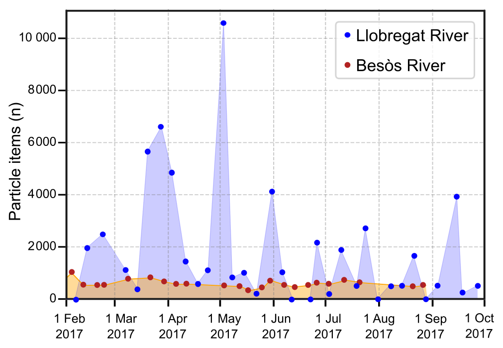
Figure A1 Linear interpolation of debris outflow from the Llobregat River and Besòs River for the period 1 February to 30 September 2017. Original data points are represented by dots in the plots.

Appendix B: Beaching parameterisation

Bosi et al. (2021)Cardoso and Caldeira (2021)Chassignet et al. (2021)Dobler et al. (2019)Kaandorp et al. (2020)Kaandorp et al. (2022)Kaandorp et al. (2023)Lebreton et al. (2012)Lebreton et al. (2019)Liubartseva et al. (2018)Macias et al. (2019)Macias et al. (2022)Mansui et al. (2015)Onink et al. (2021)Politikos et al. (2017)Politikos et al. (2020)Rosas et al. (2021)Ruiz et al. (2022)Seo and Park (2020)van der Mheen et al. (2020)Vogt-Vincent et al. (2023)Yoon et al. (2010)Zambianchi et al. (2017)Zhang et al. (2020)

Table B1 Marine debris particle beaching parameterisations and amounts in the literature. P: probabilistic. D: deterministic.

Appendix C: IBI-CMEMS node coordinates

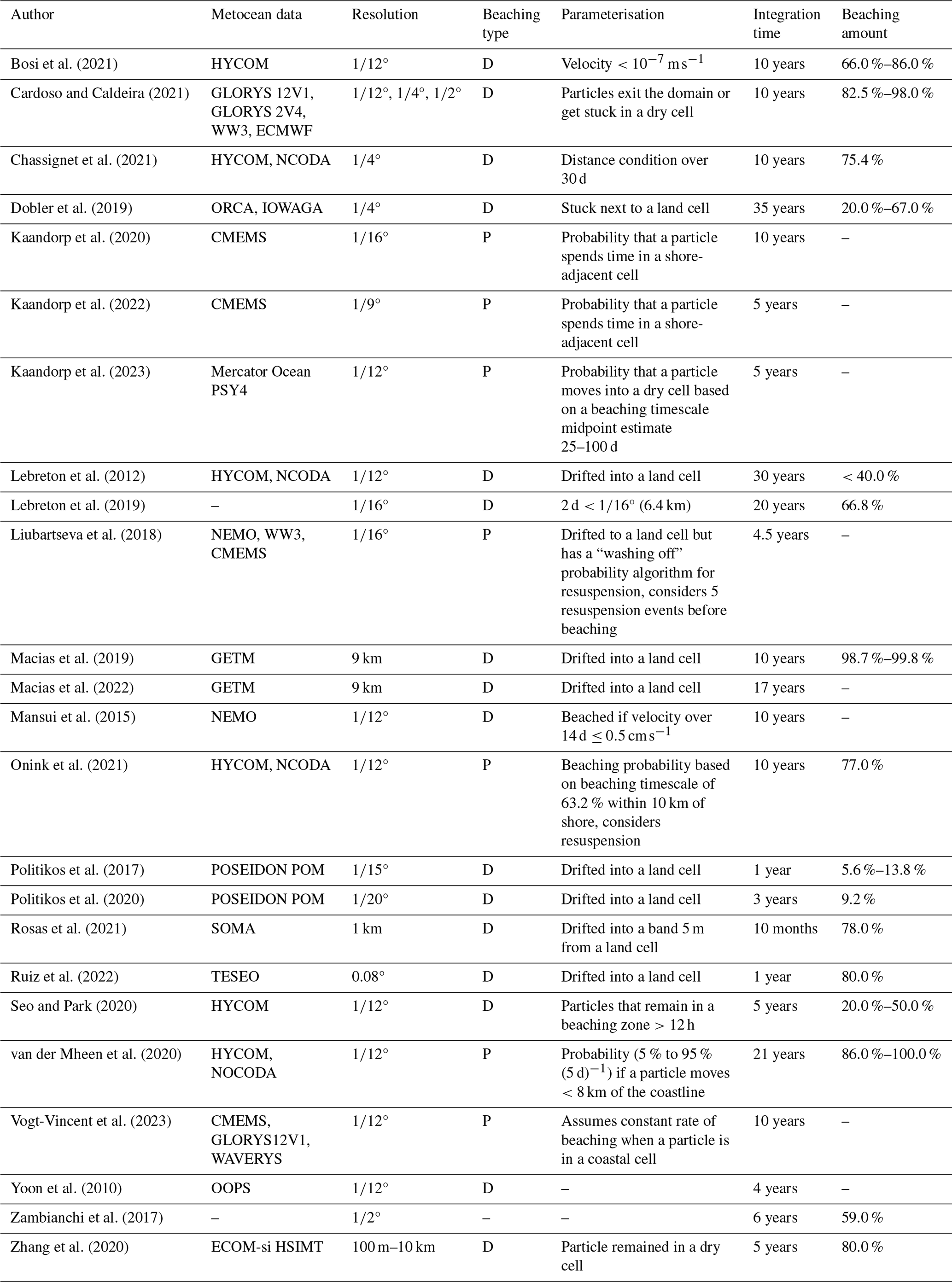
Table C1 IBI-CMEMS node coordinates used for the release of particles in the beaching sensitivity test.

Appendix D: Particle density plots

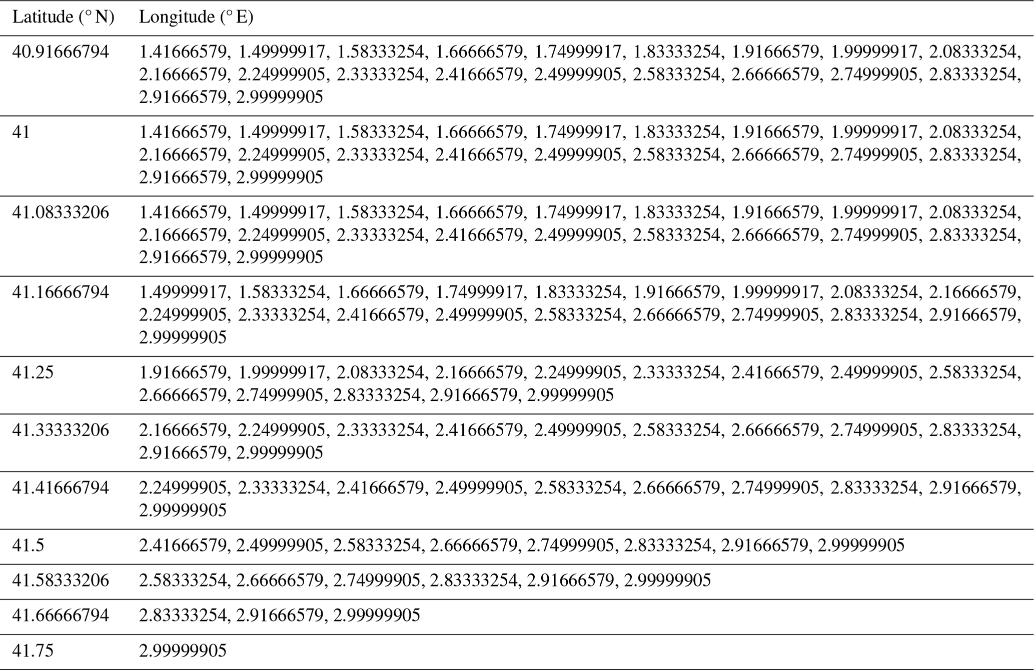
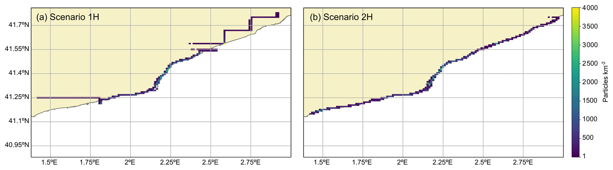
Figure D1 Particle density plots for scenarios 1 and 2 for the homogeneous particle release in the beaching sensitivity analysis. Of interest are the areas 41.25° N, 1.5° E in panel (b) which may represent artificial convergence between the hydrodynamic and real coastlines, and the area around 41.6° N, 2.6° E shows accumulation peaks of approximately 3700 particles per square kilometre (n km⁻²) in panel (a) and 2300 particles per square kilometre in panel (b).