Modelling water isotopologues (¹H²H¹⁶O, ¹H₂¹⁷O) in the coupled numerical climate model iLOVECLIM (version 1.1.5)

Stable water isotopes are used to infer changes in the hydrological cycle for different climate periods and various climatic archives. Following previous developments of δ¹⁸O in the coupled climate model of intermediate complexity, iLOVECLIM, we present here the implementation of the ¹H²H¹⁶O and ¹H₂¹⁷O water isotopes in the different components of this model and calculate the associated secondary markers deuterium excess (d-excess) and oxygen-17 excess (¹⁷O-excess) in the atmosphere and ocean. So far, the latter has only been modelled by the atmospheric model LMDZ4. Results of a 5000-year equilibrium simulation under preindustrial conditions are analysed and compared to observations and several isotope-enabled models for the atmosphere and ocean components.

In the atmospheric component, the model correctly reproduces the first-order global distribution of the δ²H and d-excess as observed in the data (R=0.56 for δ²H and 0.36 for d-excess), even if local differences are observed. The model–data correlation is within the range of other water-isotope-enabled general circulation models. The main isotopic effects and the latitudinal gradient are properly modelled, similarly to previous water-isotope-enabled general circulation model simulations, despite a simplified atmospheric component in iLOVECLIM. One exception is observed in Antarctica where the model does not correctly estimate the water isotope composition, a consequence of the non-conservative behaviour of the advection scheme at a very low moisture content. The modelled ¹⁷O-excess presents a too-important dispersion of the values in comparison to the observations and is not correctly reproduced in the model, mainly because of the complex processes involved in the ¹⁷O-excess isotopic value. For the ocean, the model simulates an adequate isotopic ratio in comparison to the observations, except for local areas such as the surface of the Arabian Sea, a part of the Arctic and the western equatorial Indian Ocean. Data–model evaluation also presents a good match for the δ²H over the entire water column in the Atlantic Ocean, reflecting the influence of the different water masses.

1 Introduction

Stable water isotopologues (¹H²H¹⁶O, ¹H₂¹⁶O, ¹H₂¹⁷O, ¹H₂¹⁸O), expressed hereafter in the usual delta notation with respect to the Vienna Standard Mean Ocean Water (V-SMOW) scale (Dansgaard, 1964), are important tracers of the hydrological cycle and are measured in a large variety of archives to reconstruct climate variations. At first order, the δ²H and δ¹⁸O of precipitation measured in polar ice cores can be used as a proxy of past temperature at the drilling site (e.g. Johnsen et al., 1972; Lorius et al., 1979; Jouzel et al., 2003). As they present the same variations, we can derive a second-order parameter called deuterium excess (d-excess) from the difference between the δ²H and δ¹⁸O. During evaporation, kinetic non-equilibrium processes affect the relationship between oxygen and hydrogen isotopes and lead to a deviation from the global meteoric water line, which represents the linear relationship between δ²H and δ¹⁸O (Craig, 1961; Dansgaard, 1964):

$$\begin{array}{}\text{(1)}& \text{d-excess}=\mathit{\delta }{}^{\mathrm{2}}\mathrm{H}-\mathrm{8}\times {\mathit{\delta }}^{\mathrm{18}}\mathrm{O}.\end{array}$$

This parameter is a classical polar ice core tracer that can be used to provide additional constraints on past climates and changes in the atmospheric water cycle. The deuterium excess is conventionally interpreted in terms of temperature at the moisture source or shifts in moisture origin (Stenni et al., 2001; Vimeux et al., 2002; Masson-Delmotte et al., 2005), even if it can also be impacted by local temperature (Masson-Delmotte et al., 2008a) and mixing along trajectory (Hendricks et al., 2000; Sodemann et al., 2008). Modelling studies, such as Risi et al. (2013), have also suggested that the d-excess is controlled by convective processes and rain re-evaporation at the tropics and by the effect of distillation and mixing between vapours from different origins at high latitudes. Recently, Landais et al. (2021) have also shown, using the first 800 000-year d-excess record, that precipitation, seasonality and moisture source region changes in the past can complicate the interpretation of the d-excess.

Following experimental developments for an accurate measurement of ¹H₂¹⁷O abundance (Barkan and Luz, 2007; Landais et al., 2008), a second-order parameter, the oxygen-17 excess (¹⁷O-excess), has been defined such as

$$\begin{array}{}\text{(2)}& {}^{\mathrm{17}}\text{O-excess}=\ln \left({\displaystyle \frac{{\mathit{\delta }}^{\mathrm{17}}\mathrm{O}}{\mathrm{1000}}}+\mathrm{1}\right)-\mathrm{0.528}\times \ln \left({\displaystyle \frac{{\mathit{\delta }}^{\mathrm{18}}\mathrm{O}}{\mathrm{1000}}}+\mathrm{1}\right).\end{array}$$

The ¹⁷O-excess is then multiplied by 10⁶ and expressed in per meg since magnitudes are very small (Landais et al., 2008). Note that we used the logarithm notation for ¹⁷O-excess following Luz and Barkan (2005). This definition makes it very sensitive to mixing between vapours of different origins (Risi et al., 2010).

The ¹⁷O-excess is commonly used in ice-core-based palaeoclimate studies to give information on the relative humidity over the ocean (e.g. Landais et al., 2008, 2018; Risi et al., 2010; Steig et al., 2021). This proxy is controlled by kinetic fractionation during evaporation and, similarly to d-excess, is very sensitive to empirical parameters determining the supersaturation in polar clouds (Landais et al., 2012; Winkler et al., 2012). Since influences of temperature or condensation altitude on ¹⁷O-excess are expected to be insignificant in contrast to d-excess, measurements of ¹⁷O-excess have an added value with respect to d-excess and can be used to disentangle the parameters (temperature, relative humidity) that affect the water isotopic composition. For example, Risi et al. (2010) have shown that the different behaviours of d-excess and ¹⁷O-excess in polar regions could be related to fractionation processes along the distillation pathway from the evaporative source to the polar region, which affect the d-excess more than the ¹⁷O-excess, with the ¹⁷O-excess recording the signal from low latitudes during surface evaporation more. Modelling the ¹⁷O-excess is still very challenging since it depends on complex processes that have to be properly reproduced in the climate models. To date, only the LMDZ4 model has included the ¹⁷O-excess (Risi et al., 2013). However, even if the processes that control the ¹⁷O-excess are more complex than those controlling the d-excess, the combination of the d-excess, ¹⁷O-excess and ¹⁸O could lead to new information on the understanding of past changes in local temperature, moisture origin and conditions at the moisture source.

Among the new proxies to document the water isotopic ratio in precipitation, the hydrogen isotope composition of plant wax (alkanes) has been found to reflect predominantly local continental rainfall fluctuations (e.g. Schefuß et al., 2005; Collins et al., 2013; Kuechler et al., 2013). Isotopic changes are primarily controlled by moisture loss by evapotranspiration, soil water conditions and precipitations rates, but the vegetation and isotopic enrichment effects should also be considered (Hou et al., 2008; Sachse et al., 2012; Kahmen et al., 2013a, b). Another method has also been developed to extract the fossil water (fluid inclusions) of speleothem records (Vonhof et al., 2006; van Breukelen et al., 2008). It then becomes possible to realize hydrogen and oxygen stable isotope analyses of fossil precipitation waters and to document the deuterium excess values in the past, outside the limited region of the ice core presence.

Similarly to continental records, the isotopologues in ocean surface waters track regional freshwater balance and then the hydrological cycle (Craig and Gordon, 1965). Water isotopologues in seawater can therefore be used as a proxy for salinity since surface freshwater exchanges are important for determining the variability of both variables. Seawater oxygen isotope concentration preserved in carbonate from organisms such as foraminifera allows for qualitative estimations of past regional changes in salinity and ocean circulation (Schmidt et al., 2007; Caley et al., 2011). It has been suggested that combining seawater hydrogen isotopes (δ²H obtained from alkenones or other biomarkers) with oxygen isotopes (δ¹⁸O obtained from zooplankton calcite shells of foraminifera) could be a promising way to quantitatively estimate salinity variability (Rohling, 2007; Legrande and Schmidt, 2011; Leduc et al., 2013; Caley and Roche, 2015).

With the emergence of new palaeoproxies to document water isotopologues in atmospheric and oceanic components of the climate system, the need to develop and use isotope-enabled models, and in particular coupled ocean–atmosphere models, has never been greater (e.g. Schmidt et al., 2007; Tindall et al., 2009; Werner et al., 2016; Cauquoin et al., 2019a). These later allow for more complex assumptions related to palaeoclimatic proxies to be examined (LeGrande and Schmidt, 2006; Schmidt et al., 2007). For example, the simulation of the climate and its associated isotopic signal can provide a “transfer function” between the isotopic signal and the considered climate variable such as the precipitation rate/water isotopes in precipitation or salinity/water isotopes in seawater relationships.

Since the initial work of Joussaume et al. (1984) and Jouzel et al. (1987), much progress has been made in atmospheric general circulation models (AGCMs) (e.g. Hoffmann et al., 1998; Noone and Simonds, 2002; Mathieu et al., 2002; Risi et al., 2010; Werner et al., 2011) that can accurately simulate the δ¹⁸O of precipitation. The subsequent development of water isotope modules in oceanic general circulation models (OGCMs) (Schmidt, 1998; Delaygue et al., 2000; Xu et al., 2012) opens the possibility of coupled simulations of present and past climates, conserving water isotopes through the hydrosphere (Schmidt et al., 2007; Zhou et al., 2008; Tindall et al., 2009; Werner et al., 2016; Cauquoin et al., 2019a). General circulation models (GCMs) had first been used to simulate water isotopes in the atmospheric and oceanic components separately but are now capable of running snapshot coupled simulations with the water isotopes enabled. However, running transient coupled simulations like the last deglaciation or the Holocene still remains challenging due to the high computing cost of these GCMs. Given the computing resources needed to run coupled climate models, applying intermediate-complexity coupled climate models with water isotopes like iLOVECLIM to long-term palaeoclimate perspectives is suitable (e.g. Caley et al., 2014). Other isotope-enabled intermediate-complexity models like CLIMBER (Roche et al., 2004) or fast GCMs like SPEEDY-IER (Dee et al., 2015) also exist, which could be used to improve our understanding of the relationship between water isotopologues, second-order parameters (like d-excess) and the climate over a broad range of simulated climate changes.

Oxygen isotopes (18, 16) have been implemented in iLOVECLIM, allowing for fully coupled atmosphere–ocean simulations. A detailed implementation of oxygen isotopes in iLOVECLIM and an evaluation against observed data in water samples and carbonates can be found in Roche (2013), Roche and Caley (2013), and Caley and Roche (2013). In the present paper, we present the design and the validation of δ²H water isotopes as well as deuterium excess and ¹⁷O-excess in the coupled climate model iLOVECLIM for the atmospheric and oceanic components. The agreements with and differences from the direct comparison between modelling results under preindustrial conditions with (1) multiple datasets and (2) several isotope-enabled GCM results for the atmosphere and ocean components are discussed to determine the potential of using iLOVECLIM in palaeoclimatic studies.

2 Description of the water isotopic scheme in iLOVECLIM

2.1 Atmospheric component ECBilt

The iLOVECLIM model (version 1.1.5) is a derivative of the LOVECLIM 1.2 climate model extensively described in Goosse et al. (2010). It is composed of an atmospheric, an oceanic, a land surface and a vegetation component. The atmospheric component ECBilt is a quasi-geostrophic model with a T21 spectral grid (resolution of 5.6° in latitude and longitude) with a complete description of the water cycle from evaporation to condensation and precipitation. The time step of the atmospheric component is 6 h. It is subdivided into three vertical layers: (1) between the surface and 650 hPa, (2) between 650 and 350 hPa, and (3) between 350 and 0 hPa. The mid-point of each layer is 800, 500 and 200 hPa respectively. The humidity is contained only in the first layer and is representative of the total humidity content of the atmosphere. Evaporative water fluxes are added to this humid layer, and vertical advection is computed. Water fluxes crossing the limit between the humid and dry layers are rained out instantly as convective rain. For specific humidity of the humid layer larger than 80 % (set as the saturation humidity at a given temperature), the excess water is removed as large-scale precipitation. If large-scale precipitation occurs with negative temperatures, excess precipitation is removed as large-scale snowfall.

With regard to water isotopes, the main development lies in the atmospheric component in which evaporation, condensation and the existence of different phases (liquid and solid) all affect the isotopic conditions of the water isotopes. The methodology used to trace the hydrogen water isotopes in ECBilt is identical to the description in Roche (2013) for the oxygen water isotopes. We used the same equations presented for the ¹⁸O in Roche (2013) but with adapted fractionation coefficients for the hydrogen and ¹⁷O. We present in this section the equations for the heavy/light isotope ratios. Additional information on the general water scheme formulation can be found in Roche (2013).

In ECBilt, the water isotopic quantity is expressed as a single tracer of water, and the humidity is assumed to be only in the first layer. For ¹H²H¹⁶O${/}^{\mathrm{1}}$H₂¹⁶O, it is defined as a function of the quantity of precipitable water for the whole atmospheric column ($\stackrel{\mathrm{̃}}{q}$, which depends on the mass of the water, the surface area of the cell and the water density) and of the ratio (R^H) between the number of moles of ¹H²H¹⁶O and the number of moles of ¹H₂¹⁶O:

$$\begin{array}{}\text{(3)}& {\stackrel{\mathrm{̃}}{q}}^{\mathrm{H}}=\stackrel{\mathrm{̃}}{q}\times R^{\mathrm{H}}.\end{array}$$

The isotopic ratio then changes within the water cycle, from evaporation to precipitation. The evaporation term for hydrogen water isotopes cannot be written in a simple manner like for the humidity because there is no vertical discretization for water isotopes in the model. The solution adopted by Roche (2013) is to compute the water isotopic ratio in the evaporation using a Craig and Gordon (1965) type-model in the formulation adapted by Cappa et al. (2003). The hydrogen isotopic ratio of evaporating moisture can then be written as

$$\begin{array}{}\text{(4)}& R_{\mathrm{E}}^{\mathrm{H}}={\mathit{\alpha }}_{\mathrm{diff}}^{\ast }\left({\displaystyle \frac{R_{\mathrm{eq}}^{\mathrm{H}}-h_{\mathrm{a}}^{\ast }{R}_{\mathrm{a}}^{\mathrm{H}}}{\mathrm{1}-h_{\mathrm{a}}^{\ast }}}\right),\end{array}$$

where $R_{\mathrm{eq}}^{\mathrm{H}}$ is the isotopic ratio at equilibrium with the ocean, $R_{\mathrm{a}}^{\mathrm{H}}$ is the isotopic ratio of the humidity in the atmosphere and $h_{\mathrm{a}}^{\ast }$ is an apparent relative humidity value for the atmosphere. ${\mathit{\alpha }}_{\mathrm{diff}}^{\ast }$ is a ratio of molecular diffusivity and is defined for the hydrogen such as

$$\begin{array}{}\text{(5)}& {\mathit{\alpha }}_{\mathrm{diff}}^{\ast }={\left({\displaystyle \frac{D^{\mathrm{H}}}{D}}\right)}^n,\end{array}$$

where D^H is the molecular diffusivity of water ¹H²H¹⁶O, D is the molecular diffusivity of water ¹H₂¹⁶O and n is a coefficient that varies with turbulence and evaporative surface (Brutsaert, 1975; Mathieu and Bariac, 1996). The molecular diffusivity ratio for ¹H²H¹⁶O${/}^{\mathrm{1}}$H₂¹⁶O is set to 0.9755 (Merlivat, 1978) and 0.9855 for ¹H₂¹⁷O${/}^{\mathrm{1}}$H₂¹⁶O (Barkan and Luz, 2007).

Since ECBilt only includes three layers, it is supposed that precipitation always forms in isotopic equilibrium with the surrounding moisture with instantaneous rainout to the surface. The convective precipitations, large-scale precipitation and snow are in equilibrium with isotopic values (using temperature at 650, 800 and 650 hPa respectively). When computing the precipitation and snow fractionation coefficients (see Roche, 2013), we take into account the temperature, the equilibrium fractionation coefficients between the different water phases for the hydrogen (Merlivat and Jouzel, 1979) and the ratio of hydrogen isotopes in vapour. In these equations, the hydrogen equilibrium fractionation coefficient between liquid water and vapour is taken from Majoube (1971a) and depends on the temperature:

$$\begin{array}{}\text{(6)}& {\mathit{\alpha }}_{\mathrm{l}-\mathrm{v}}^{\mathrm{H}}=\exp \left({\displaystyle \frac{\mathrm{24}\mathrm{844}}{T^{\mathrm{2}}}}-{\displaystyle \frac{\mathrm{76.248}}{T}}+\mathrm{0.052612}\right).\end{array}$$

For ¹⁷O, the fractionation between liquid water and vapour is calculated from Majoube (1971a) and Barkan and Luz (2005, 2007):

$$\begin{array}{}\text{(7)}& {\mathit{\alpha }}_{\mathrm{l}-\mathrm{v}}^{\mathrm{O}}=\exp \left({\displaystyle \frac{\mathrm{1137}}{T^{\mathrm{2}}}}-{\displaystyle \frac{\mathrm{0.4156}}{T}}-\mathrm{0.0020667}\right)\times \mathrm{0.529}.\end{array}$$

The equilibrium fractionation coefficient between solid water and water vapour for hydrogen is taken from Merlivat and Nief (1967) and depends on the temperature as well:

$$\begin{array}{}\text{(8)}& {\mathit{\alpha }}_{\mathrm{s}-\mathrm{v}}^{\mathrm{H}}=\exp \left({\displaystyle \frac{\mathrm{16}\mathrm{289}}{T^{\mathrm{2}}}}-\mathrm{0.0945}\right).\end{array}$$

For ¹⁷O, the fractionation between solid water and vapour is calculated from Majoube (1971b) and Barkan and Luz (2005, 2007):

$$\begin{array}{}\text{(9)}& {\mathit{\alpha }}_{\mathrm{s}-\mathrm{v}}^{\mathrm{O}}=\exp \left({\displaystyle \frac{\mathrm{11.839}}{T^{\mathrm{2}}}}-\mathrm{0.028224}\right)\times \mathrm{0.528}.\end{array}$$

2.2 Ocean and land surface components

The oceanic component CLIO has a 3 × 3° horizontal resolution, 20 vertical layers and a free surface. All the variables are calculated with a daily time step. In the ocean, the water isotopes are mass conserving and act as passive tracers under equilibrium fractionation, ignoring the small fractionation implied by the presence of sea ice (Craig and Gordon, 1965).

For the land surface model, the isotope water implementation in the bucket follows the same procedure as for the water. If re-evaporation occurs on land, it is assumed to be at equilibrium (without fractionation). A snow layer is also taken into account. Above a given threshold, the isotopic water and snow contents in the soil and snow buckets are routed to the ocean without fractionation.

2.3 Simulation setup

We present results of a 5000-year equilibrium run under fixed preindustrial boundary conditions. The atmospheric pCO₂ is set to 280 ppm, the methane concentration is 760 ppb and the nitrous oxide concentration is 270 ppb. The orbital configuration is calculated from Berger (1978) with 1950 as a constant year. We use present-day land–sea masks, freshwater routing and interactive vegetation. With regard to the water isotopes, the atmospheric moisture is initialized at 0 and δ²H at 0 ‰. The consistency of our integration is checked by ensuring that the water isotopes are fully conserved in our coupled system. The model has been run at T21 spatial resolution, and the outputs are computed with an annual time step.

To investigate the seasonal variations in the model in comparison to the observations and to estimate the range of the modelled results, we performed a 100-year simulation starting from the equilibrium run, with monthly outputs for the climate and the isotopes. This simulation is investigated in Sect. 3.1.4.

2.4 Observational data and water-isotope-enabled GCMs

To allow for comparison with and discussion of iLOVECLIM results, global hydrogen and d-excess isotopic datasets for the atmosphere from the Global Network of Isotopes in Precipitation (GNIP) dataset (IAEA, 2023) and Masson-Delmotte et al. (2008b) have been used. The original GNIP dataset has been subsampled to keep only the stations where the isotopic composition has been reported for a minimum of 3 calendar years within the 1961–2008 period. To evaluate the seasonal evolution of the model, we looked at the evolution of precipitations and the atmospheric isotopic ratio at several locations distributed on multiple continents to reflect the variety of climate: Pretoria (25.73° S, 28.18° E), Belem (1.43° S, 48.48° W), Ankara (39.95° N, 32.88° E) and Reykjavik (64.13° N, 21.92° W). Present-day measurements of δ¹⁷O and ¹⁷O-excess from multiple studies (Landais et al., 2008, 2010, 2012; Luz and Barkan, 2010; Uemura et al., 2010; Winkler et al., 2012; Pang et al., 2015; Tian et al., 2021; IAEA, 2023) have been used. Note that the data of Uemura et al. (2010) are for the vapour and not the precipitation and do not allow for a direct model–data comparison.

The GISS global seawater isotope database (Schmidt et al., 1999) has been used to compare the δ²H and d-excess with the ocean component in the model. We looked at the surface distribution of the isotopes for the first oceanic layer at 5 m depth in the model and selected GISS seawater values between 0 and 10 m to be representative of the surface.

To evaluate our model results against water-isotope-enabled GCMs, we used several model outputs: ECHAM5-wiso (Steiger et al., 2017; Steiger, 2018), GISS (Schmidt et al., 2007), LMDZ4 (Risi et al., 2010, 2013), MIROC (Kurita et al., 2011), CAM (Lee et al., 2007) and MPI-ESM-wiso (Cauquoin et al., 2020). The GISS, LMDZ4, MIROC and CAM data are from the Stable Water Isotope Intercomparison Group Phase 2 (SWING2) (Risi et al., 2012). δ²H_seawater in MPI-ESM-wiso has been calculated from δ¹⁸O_seawater and d-excess outputs.

3 Results and discussion

3.1 Water isotopic composition in the atmosphere

3.1.1 Annual δ²H_{precipitation}

The annual-mean modelled distribution of δ²H_{precipitation} is presented in comparison to observations in Fig. 1a. The latitudinal gradient from the poles to the Equator is correctly reproduced in the model, with low values at high latitudes (cold and dry regions) and high values at lower latitudes. However, regions like central Africa and the northern region of South America are different from the data since the modelled δ²H_{precipitation} is underestimated in comparison to the few measurements available. This could be due to one of the well-known iLOVECLIM biases – the overestimation of the precipitation in these regions. The west coast of South America also presents discrepancies between the model and the GNIP data (Fig. 1a). This could be related to the coarse model resolution that may not perfectly reproduce the observed δ²H_{precipitation} since the value is representative of a larger area. Finally, the modelled δ²H_{precipitation} over northern America and Europe is higher than that of the observations. However, the difference in the atmospheric isotopic ratio of precipitation over land and the ocean is well reproduced in the model, with values close to 0 over the Pacific, Atlantic and Indian oceans and values lower than −50 ‰ and −80 ‰ over the Arctic and Austral oceans respectively (Fig. 1a).

We also compared the zonal distribution of several water-isotope-enabled GCMs for results that co-locate with observations. From middle to low latitudes, all models show similar δ²H_{precipitation}, with iLOVECLIM being higher than the other GCMs below 20° S and above 30° N. Despite these biases, iLOVECLIM reproduces the global trend of low values at high latitudes and high values at low latitudes, as observed in the data (Fig. 2a). At high latitudes, iLOVECLIM models an isotopic ratio that is too high compared to the one in the ECHAM5-wiso, GISS, LMDZ4, MIROC and CAM models, as well as in the GNIP data, with values between up to −453 ‰ (Fig. 2a). These very low measured values over Antarctica can be explained by the low temperature (with a continental effect) and other influences like moisture transport or the distance from the coast that add complexity in modelling this region. Since iLOVECLIM only has 3 vertical layers in comparison to the 19 to 26 vertical layers for the other GCMs, we cannot properly reproduce the isotopic variations at these latitudes as a consequence of the non-conservative behaviour of the advection scheme at a very low moisture content. However, no model is able to correctly reproduce these very low values as observed in the measurements. All the GCMs model higher values, between −305 ‰ and −365 ‰.

In order to further evaluate our model results against water-isotope-enabled models and the observations, we analysed the standard deviation (SD), correlation (R) and root mean square error (RMSE), combined in a Taylor diagram (Fig. 3). In all these figure panels, we removed Antarctic values for the reason explained above. We observe for the δ²H_{precipitation} that ECHAM5-wiso is the model that has the best correlation coefficient with the observation (R=0.64 vs R=0.56 for iLOVECLIM – Fig. 3a). The different GCMs have a close correlation coefficient (between 0.59 and 0.64), standard deviation (between 40.21 and 46.43) and RMSE (between 34.94 and 39.82). The iLOVECLIM model presents a lower standard deviation (SD = 29.93) and RMSE than the other models (Fig. 3a). However, considering the close metrics between all models, iLOVECLIM presents the advantage of running faster than the other GCMs and is thus perfectly justified for its use in long-term global climate simulations.

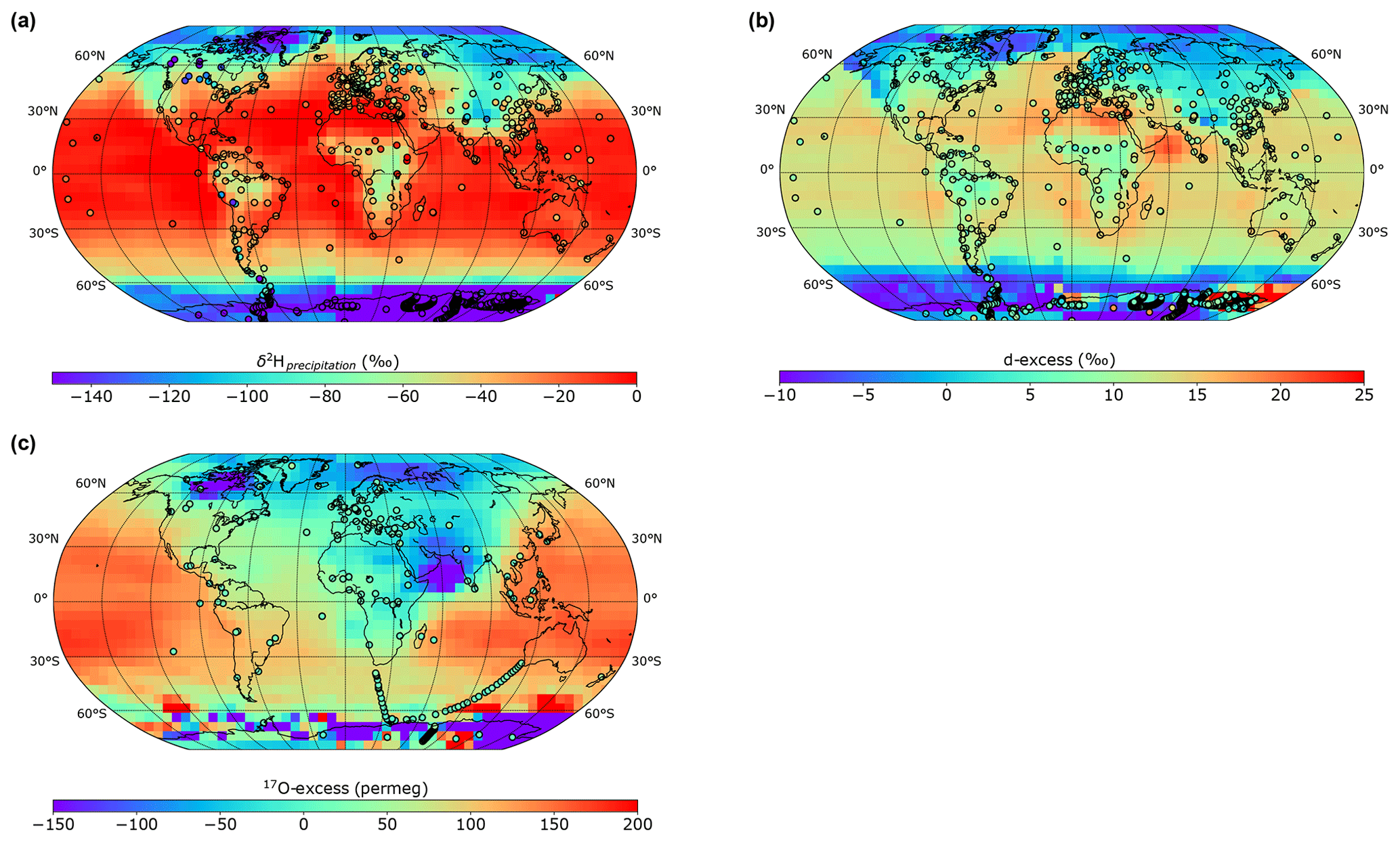
Figure 1 Model–data evaluation of the annual-mean isotope distributions. (a) δ²H in precipitation, (b) d-excess and (c) ¹⁷O-excess in iLOVECLIM. The model results are compared to observations (in circles).

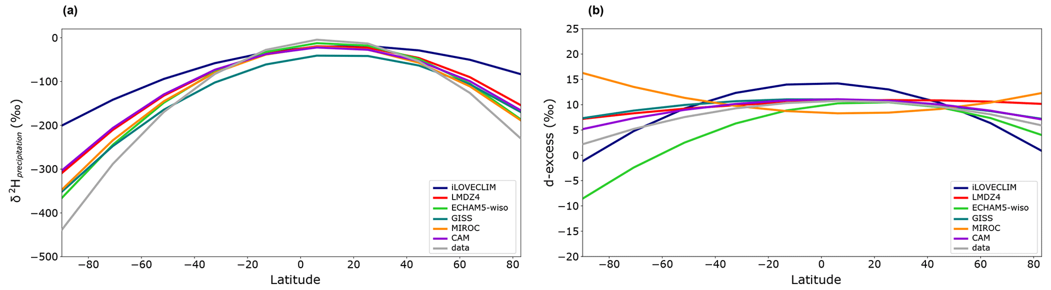
Figure 2 Multi-model zonal (a) δ²H_{precipitation} and (b) d-excess comparison. The model results (in colour) are compared to observations (in grey). The different lines are polynomial regression curves for the model results that co-locate with the observations.

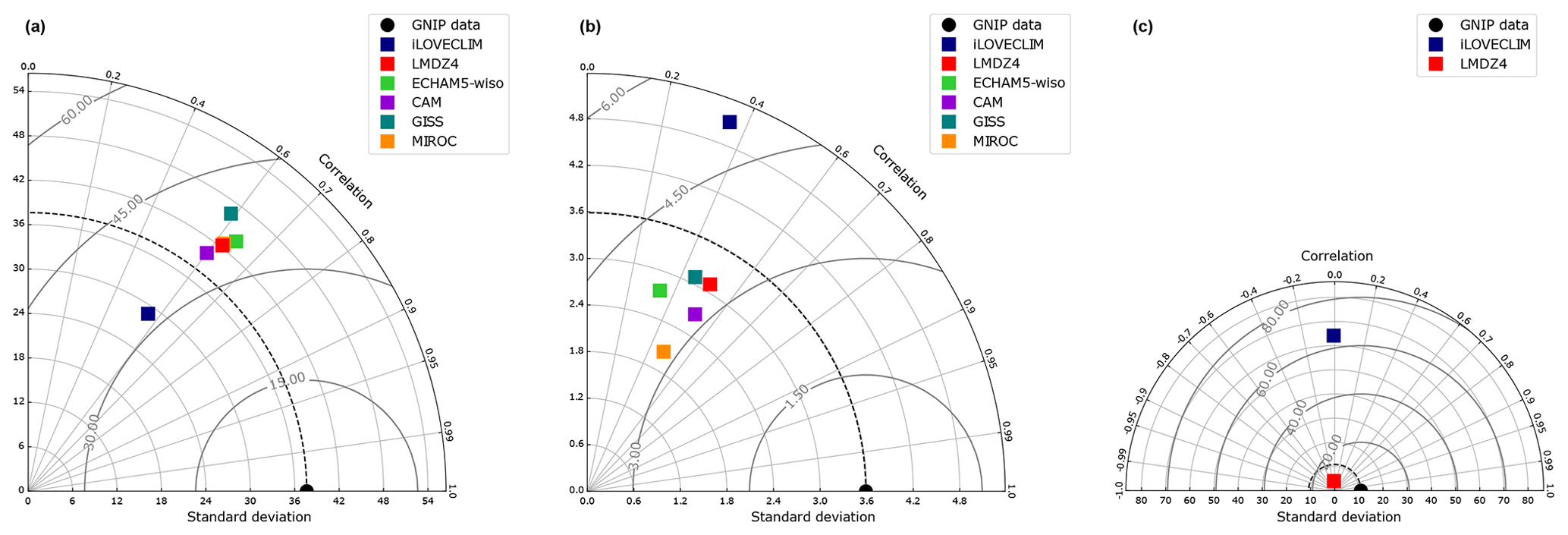
Figure 3 Taylor diagram representing (a) δ²H_{precipitation}, (b) d-excess and (c) ¹⁷O-excess values for different climate models (iLOVECLIM, LMDZ4, ECHAM5-wiso, CAM, GISS and MIROC) without Antarctic values. The simulated values are plotted against the observations. The dotted curved line indicates the reference line (standard deviation of the observations), and the bold grey contours represent RMSE values.

The linear relationship between δ¹⁸O and δ²H (δ²H$=\mathrm{8}\times {\mathit{\delta }}^{\mathrm{18}}$O + 10), established by Craig (1961) and defined as the global meteorological water line, can also be verified in the model. The model values match the GNIP observations and correctly reproduce the linear trend between the δ¹⁸O and δ²H of precipitation with a correlation coefficient of 0.99.

3.1.2 Annual deuterium excess

The annual-mean d-excess distribution is derived from the oxygen and hydrogen isotopic ratio. To evaluate the accuracy of the model, we compare the model results to the observations. As observed for δ²H_{precipitation}, the d-excess presents a latitudinal gradient with low negative values to the poles and high positive values to the Equator (Figs. 1b and 2b). The modelled values fit well with the observations at global scale. Differences between the model and the observations remain for some regions, like over India where the modelled d-excess is slightly higher than the observations. More generally, iLOVECLIM models too high d-excess values from middle to low latitudes (Fig. 2b). The modelled d-excess over Greenland, and especially the coastal areas, is negative, whereas the few available data points indicate positive values that are up to 20 ‰ higher. Similarly to the annual δ²H_{precipitation} distribution, the d-excess over Antarctica is not correctly reproduced in the model and presents outlier values in the coastal regions. The local data show values between 5 ‰ and 10 ‰, whereas the model calculates values ranging from −10 ‰ to 25 ‰ or higher in the region of Adélie Land (Fig. 1b). In Fig. 2b, we excluded these outlier values for a more suitable model intercomparison. Zonal mean d-excess values from middle to high latitudes modelled by LMDZ4, GISS and CAM are too high compared to the observations, whereas values from ECHAM5-wiso are systematically too low. The MIROC model is the only one that shows a different trend in the zonal distribution of the d-excess, with higher values in the high latitudes and low values to the Equator. Over the ocean, few d-excess data points are available, but the model presents overall good agreement with the GNIP data with mean values ranging from −10 ‰ over the Arctic and Austral oceans to 17 ‰ over the Atlantic and Pacific oceans. A maximum in d-excess is reached over the Arabian Sea with 20.6 ‰.

In comparison to the measurements for the atmosphere, iLOVECLIM has a correlation coefficient that is within the range of other models (0.34 to 0.52) but with a higher SD compared to the observations and other GCMs. The CAM model has the best correlation coefficient with the observations, whereas LMDZ4 has the closest standard deviation relative to the observations (Fig. 3b). Within all models, MIROC is the one with the lowest SD and RMSE. However, considering the general low correlation coefficient for all models, they all do not perfectly reproduce the d-excess variations as observed in the data. However, iLOVECLIM presents the advantage of running faster than the other GCMs. The same caution should be required for iLOVECLIM as for the other GCMs when investigating past changes in d-excess.

The relationship between the d-excess and δ²H_{precipitation} can be investigated and shows that it is partially driven by high-latitude values, mainly in Antarctica, as presented in Fig. 4. From the globally available data, a relationship between d-excess and δ²H_{precipitation} exists, with a high d-excess value (∼ 15 ‰) for very low δ²H_{precipitation} values (around −400 ‰ and 0 ‰), whereas lower d-excess is observed for mean δ²H_{precipitation} between −250 ‰ and −300 ‰. The low δ²H_{precipitation} values correspond to high-latitude values, mostly corresponding to Antarctic values, which drive the relationship between d-excess and δ²H_{precipitation} (R²=0.50 when considering all values, R²=0.10 for values without the high latitudes). A similar relationship between the d-excess and δ²H_{precipitation} is observed in the iLOVECLIM model. The highest d-excess values are obtained for low δ²H_{precipitation} values (around −200 ‰) and lower d-excess for intermediate δ²H_{precipitation} (Fig. 4). However, the shape of the regression curves is different between the data and the model because of outlier modelled d-excess values that are too high in the model. These data points mainly correspond to Antarctic values as already observed in Fig. 1.

Antarctic isotopic values are not computed correctly due to issues in the conservation of water in the advection scheme at a very low humidity content, a fact that has already been highlighted in Roche (2013). Improving the conservation in the spectral advection scheme is beyond the scope of the present study. We thus removed these Antarctic values in the following to investigate the isotopic trend without the influence of this region. This results in a better agreement between the data and iLOVECLIM model (with a correlation coefficient of 0.71), even if differences are observed with generally lower d-excess values in the model than in the data for low δ²H_{precipitation} (Fig. 4).

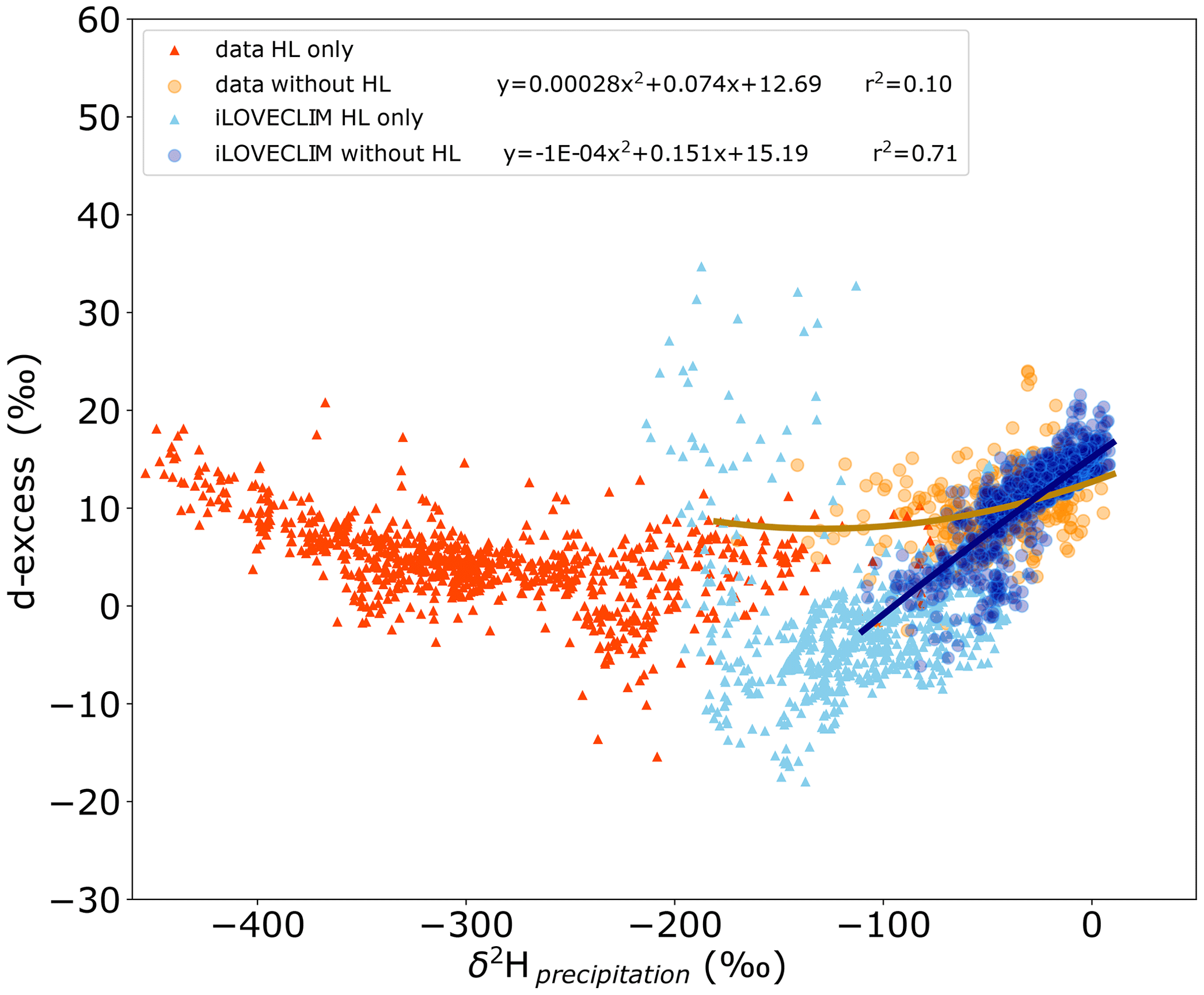
Figure 4 Global relationship between d-excess and δ²H in precipitation. High-latitude values (above 60° N and below 60° S) are presented with the red triangles for the data and with the light blue triangles for iLOVECLIM. Data for other regions are presented with the orange circles for the measurements and with the dark blue circles for the model. Regression curves for the data and the model, without high-latitude values, are also shown in orange and dark blue.

For the d-excess, the range of modelled values can be large for some locations (as already seen in Fig. 1). Thus, we can evaluate the ability of the model to reproduce the d-excess in comparison to the observed data, as presented in Fig. 5. The distribution of most d-excess values is centred around values between 8 ‰–18 ‰. A low correlation coefficient is obtained due to outlier d-excess values, but statistical significance between the model and the data is obtained with a p value of $\mathrm{3}\times {\mathrm{10}}^{-\mathrm{4}}$ (<0.001). This attests to a good representation of the d-excess in the model (excluding Antarctic values). This is also supported by the modelled d-excess in LMDZ4 that presents similar values than in iLOVECLIM (Fig. 5). However, considering the larger dispersion of the values in our model compared to LMDZ4 and to the fact that the uncertainties in the d-excess measurements are large, the relationship between the model and data might vary and become closer to the expected 1:1 line.

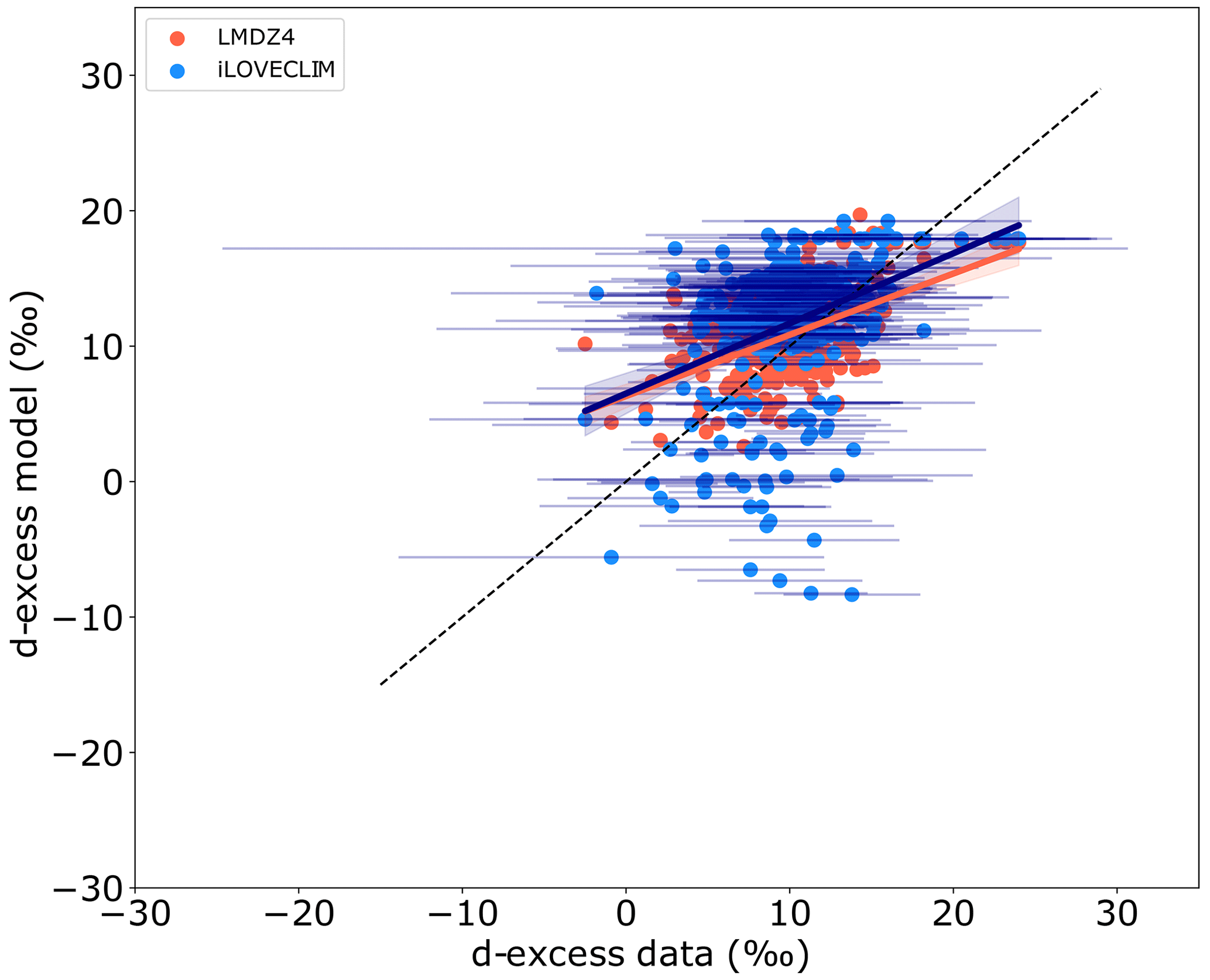
Figure 5 Relationship between the modelled d-excess in iLOVECLIM (blue) and in LMDZ4 (red) versus measurements without Antarctic values. The error bars associated with the data are shown at 2σ. The 1:1 line is shown with the dashed black line. The regression lines for iLOVECLIM and LMDZ4 are in dark blue and red respectively with the confidence bands.

3.1.3 ¹⁷O-excess distribution

The modelled ¹⁷O-excess shares a common pattern with δ¹⁷O (itself presenting the same spatial pattern as δ¹⁸O; see Appendix A), with low values over the high latitudes of the Northern Hemisphere and higher values over land (Fig. 1c). The ¹⁷O-excess presents values between 0 and 100 per meg over the Atlantic Ocean, which are lower than in the Indian and Pacific oceans. In comparison to the LMDZ4 model that is currently the only GCM that includes ¹H₂¹⁷O (Risi et al., 2013), iLOVECLIM presents higher values for most of the latitudes due to these high values over the ocean. The latitudinal gradient is also larger than in LMDZ4 that has relatively homogenous values between 70° S and 90° N. The model reproduces ¹⁷O-excess values that are close to observations over North America, Europe and Africa (Fig. 1c). But ¹⁷O-excess over the Arabian Sea and northern Canada probably has too-negative values. Similarly to d-excess and due to the outlined problem in modelling this region, the ¹⁷O-excess modelled over Antarctica presents a wide range of values from high negative to high positive and does not fit with ice core measurements.

Comparison can be done between the models and observations for the ¹⁷O-excess (Fig. 6a). A wide dispersion of the ¹⁷O-excess values (excluding values in Antarctica) is observed in the model, but they are statistically significant with a p value of 0.041 (<0.05). Higher values than observations are modelled from middle to low latitudes and lower values than observations at high latitudes of the Northern Hemisphere (Fig. 6b). ¹⁷O-excess has previously been modelled in LMDZ4 (Risi et al., 2013), with a lower dispersion of the values than in iLOVECLIM but no clear trend as expected from the data (Fig. 6a). We observe for the ¹⁷O-excess a low negative correlation coefficient for iLOVECLIM and LMDZ4 with respect to observations. Interestingly, the opposite pattern in the models compared to observations suggests that the physical processes at play are not fully understood and require further investigation. The standard deviation and root mean square error is better for LMDZ4 than for iLOVECLIM (Fig. 3c), suggesting that our model does not correctly reproduce the ¹⁷O-excess and has a too-important dispersion of the values.

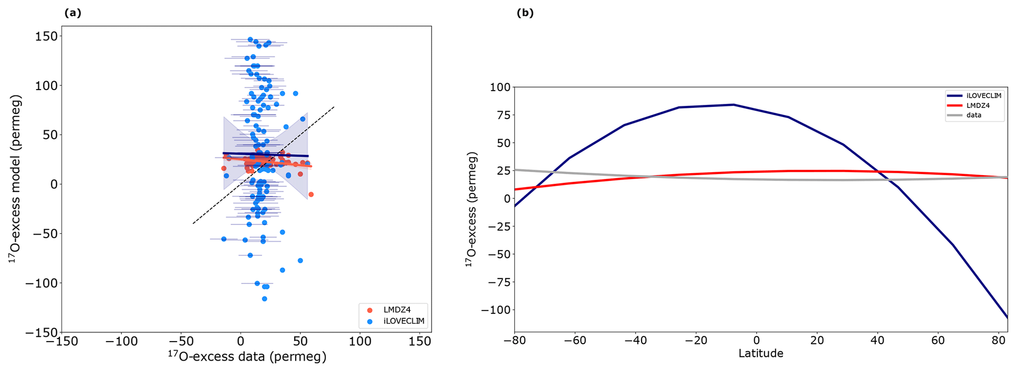
Figure 6 (a) Relationship between the iLOVECLIM-modelled isotopic value and ¹⁷O-excess measurements, without values from Antarctica. The LMDZ4 model results are also presented. The regression curves between the model and data are presented in dark blue for iLOVECLIM and red for LMDZ4 with the confidence bands. The 1:1 line is shown with the dashed black line. The error bars associated with the data are shown at 1σ. (b) Zonal ¹⁷O-excess comparison. The model results (in colour) are compared to observations (in grey). The different lines are polynomial regression curves for the model results that co-locate with the observations.

3.1.4 Seasonal variations

We compare the seasonal model results for precipitation, δ²H_{precipitation}, d-excess and ¹⁷O-excess to the GNIP monthly data at several locations representative of various climate conditions to have a global overview: South Africa (Pretoria), South America (Belem), the eastern Mediterranean (Ankara) and the northern Atlantic (Reykjavik). ¹⁷O-excess values are presented only for Ankara and Reykjavik, since no data are available for the other stations. We extracted the model results at the corresponding locations, but due to the coarse resolution of the model, regional biases exist as depicted in the previous section. We performed a mean over the last 10 years of the simulation and normalized the results (we subtracted the annual mean and divided it by the standard deviation for each station) for easier comparison with the data. The seasonal evolution of precipitation and the isotopic ratio in the model is then not expected to perfectly reflect the measurements. We then present the normalized values for both model and GNIP data.

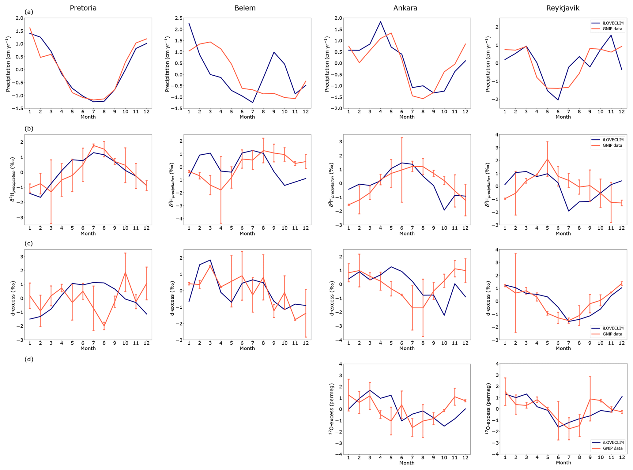
Figure 7 Monthly evolution of (a) precipitation, (b) δ²H_{precipitation}, (c) d-excess and (d) ¹⁷O-excess at several stations (different columns for Pretoria, Belem, Ankara and Reykjavik). The red line is the GNIP data measured at the station, and the blue line is the iLOVECLIM model result at the corresponding location. The data and model results have been normalized. The error bars for the data are also shown at 2σ.

There is good agreement in precipitation in Pretoria and Ankara between the observation and the model that correctly reproduces the seasonal cycle (Fig. 7a). For the Belem and Reykjavik stations, the model shows some differences, namely higher precipitations in September and October in Belem and higher monthly amplitude in Reykjavik. Good correlation is observed for the modelled δ²H_{precipitation} in comparison to observations in Pretoria and Ankara (even if the October value is very low). As for precipitations, the amplitude of δ²H_{precipitation} variations is different between the model and the data in Belem and Reykjavik (Fig. 7b). But the overall model behaviour in reproducing seasonal variations in δ²H_{precipitation} can be validated based on these observations, especially when considering that the uncertainties associated with the data can be as large as the measurement itself. However, the d-excess variations show larger differences between the model and the observations. The modelled d-excess in Reykjavik shows good agreement with the observation, while a larger amplitude of the variations is observed in Belem (Fig. 7c). In Ankara, the modelled d-excess is delayed during summer compared to observations and shows too-low values in October. In Pretoria, even if the δ²H_{precipitation} is correctly reproduced in the model, the d-excess presents differences with high values between May and September, whereas the data indicate lower values during this period. For the ¹⁷O-excess, the model–data agreement is not perfect, especially for Ankara, but the model is able to reproduce the seasonal variations as observed in the data for Reykjavik (Fig. 7d). All these model–data differences could be the result of uncertainties associated with the GNIP data and/or with biases in modelling the isotopic composition.

3.2 Evaluation of the main isotopic effects

3.2.1 Amount effect

The amount effect can be defined as a decrease in the isotopic ratio for an increase in the precipitation amount. Note that in our model the amount effect depletion is the process related to sequential precipitation removal and under-replenishment, in the form identified by Dansgaard (1964). This approach is more comparable to that of Moore et al. (2014) than the more complex approach of Risi et al. (2021). Comparing the different approaches would require further investigation and is beyond the scope of this paper.

We investigate this effect in the model and compare it to LMDZ4 and observations. We only extracted values in the models and for the GNIP stations that cover the tropics, from 0–20° N and 0–20° S, because this is where the amount effect is observed. For an easier comparison, we normalized the values (for more information, the raw values are presented in Appendix B).

The seasonal cycle in iLOVECLIM is well reproduced and in agreement with the GNIP data (especially for the precipitations between 0–20° S). In the northern tropics (Fig. 8a), the isotopic ratio of the precipitation of iLOVECLIM is lower during the wet season (i.e. during the boreal summer). The opposite effect is observed in the southern tropics (Fig. 8b), with high δ²H_{precipitation} during the austral winter, associated with a reduced amount of precipitation. Thus, δ²H_{precipitation} decreases as precipitation intensity increases. In the model, the minimum δ²H_{precipitation} leads the minimum observed for the GNIP stations of 1 month, whereas the minimum δ²H_{precipitation} in LMDZ4 lags the observations of 1 month for the northern tropics.

We further investigate this amount effect by examining the change in the δ²H_{precipitation} as a function of the amount of precipitation. Following Risi et al. (2008, 2010), we looked at the seasonal model variations for nine oceanic tropical GNIP stations (Apia, Barbados, Canton Island, Diego Garcia, Madang, Taguac, Chuuk (previously Truk), Wake Island and Yap). Because the resolution in iLOVECLIM is T21, the local processes may not be perfectly reproduced, and the comparison to local oceanic observations is complicated. Therefore, we selected for each GNIP station the pixel that was in better agreement with the precipitation and isotopic ratio seasonal cycle data. We also do not present observational precipitation values above 350 cm yr⁻¹ since in the model precipitations are never higher.

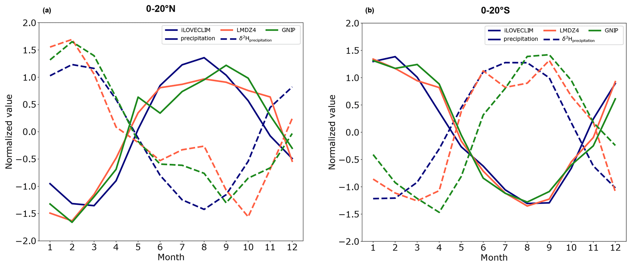
Figure 8 Seasonal variations in the mean precipitation and δ²H_{precipitation} in the tropics, from 0–20° N (a) and 0–20° S (b). The values have been normalized. The solid lines represent the precipitation and the dashed lines the δ²H_{precipitation}. The blue curve presents the iLOVECLIM values, the red curve is for LMDZ4 and the green curve corresponds to the GNIP data.

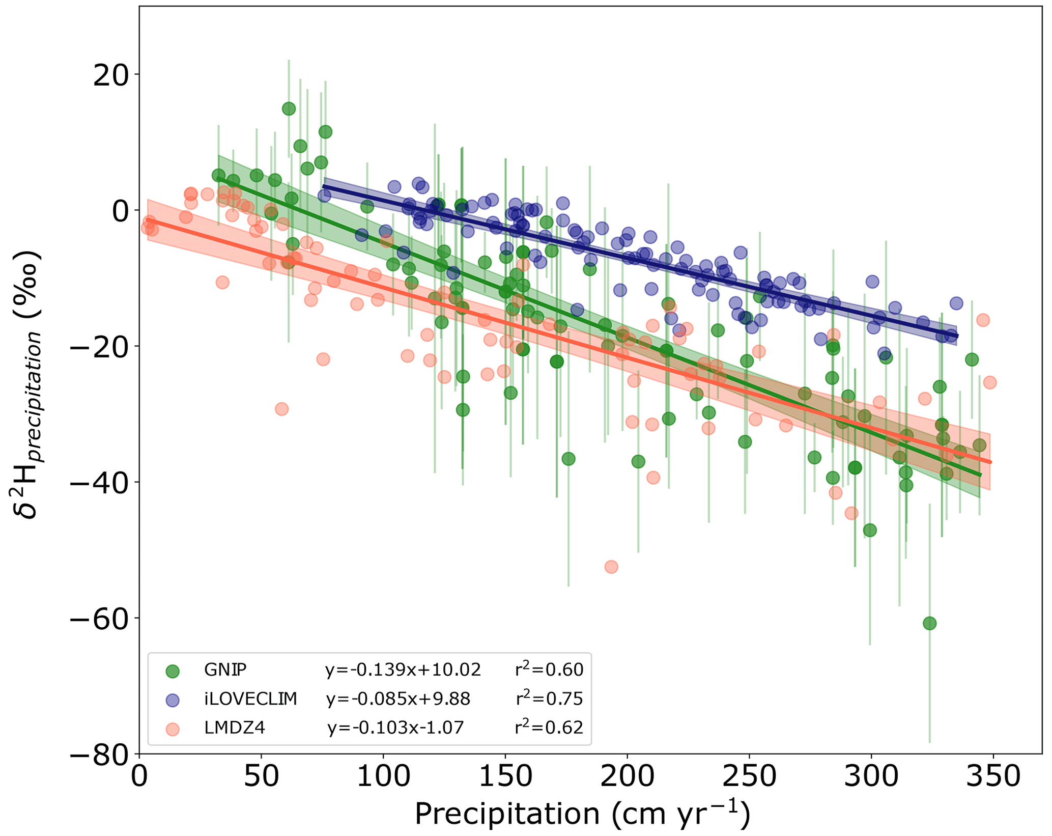
Figure 9 Monthly δ²H_{precipitation} as a function of the precipitation at the location of nine tropical oceanic GNIP stations. The iLOVECLIM results in blue are compared to LMDZ4 results in red and GNIP data in green. The error bars for the data are shown at 2σ.

Figure 9 presents the relationship between the δ²H_{precipitation} and the precipitation for the selected stations in iLOVECLIM, the observations and LMDZ4. The isotopic ratio of precipitation is high for low precipitations and changes toward low values as precipitations increase. This amount effect is −0.085 ‰ cm⁻¹ yr⁻¹ in iLOVECLIM, weaker than the one observed in LMDZ4 (−0.103 ‰ cm⁻¹ yr⁻¹) and in GNIP data (−0.139 ‰ cm⁻¹ yr⁻¹). The modelled δ²H_{precipitation} is however higher than the observations for the same precipitation amount (especially at high precipitations). In contrast, the standard version of LMDZ4 has slightly lower δ²H_{precipitation} at low precipitations in comparison to the observations, as has already been noted by Risi et al. (2010).

3.2.2 Temperature effect

Temperature plays an important role in the hydrogen isotopic ratio of precipitation with lower values for low temperatures. We investigate in this section this relationship in iLOVECLIM and compare it to the LMDZ4 model. Since in our model the surface temperature is not a prognostic variable, we used the temperature at 650 hPa (top of the first layer) and took the equivalent temperature in the LMDZ4 model at 662 hPa. An enhanced depletion of the δ²H_{precipitation} is observed with a decrease in the temperature in both models (Fig. 10a). However, differences are noticed at low temperatures (below −15 °C), mainly corresponding to Antarctic values, with an isotopic ratio that is not low enough in our model. Antarctic isotopic values are indeed not computed correctly due to issues in the conservation of water in the advection scheme at a very low humidity content, as has already been highlighted in Roche (2013). We then investigate the relationship between modelled and measured δ²H_{precipitation}, excluding Antarctic values (Fig. 10b). Most of the values are found between 0 ‰ and −60 ‰, with a similar distribution in iLOVECLIM and LMDZ4. Differences in modelled δ²H_{precipitation} between iLOVECLIM and LMDZ4 are enhanced for the lower values, and model–data agreement is deteriorated. As shown in Cauquoin et al. (2019b), the representation of the advection scheme in the model can impact the isotopic composition, with more enriched values when a more diffusive advection scheme is applied.

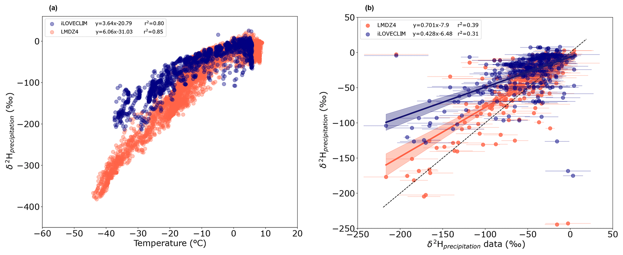
Figure 10 (a) Annual-mean modelled δ²H_{precipitation} as a function of the temperature for iLOVECLIM (blue) and LMDZ4 (red). (b) Annual-mean modelled δ²H_{precipitation} for iLOVECLIM and LMDZ4 against observations (without Antarctic values). The 1:1 line is shown with the dashed black line. The error bars associated with the data are shown at 2σ. The regression curves between the models and data are presented in dark blue for iLOVECLIM and red for LMDZ4 with the confidence bands.

3.2.3 Continental effect

The continental effect can be defined by a contrast in isotopic values between land and the ocean, with lower values over land (Rozanski et al., 1993). To evaluate this effect in iLOVECLIM, we extracted the monthly isotopic ratio of precipitation over land and the ocean separately and focused first on the tropics between 0–20° N and 0–20° S and second on the middle to high latitudes between 40–70° N. We also extracted values from the LMDZ4 and ECHAM5-wiso models and from the GNIP stations that have at least three measurements for each month. The total number of points/stations over the continents and oceans for each model (increasing with a higher resolution of the model) and observation is summarized in Table 1. Instead of representing all data points, we decided to show the monthly mean values that correspond to the continents (America, Africa and Asia/Indonesia/Australia for the tropics; Europe, Asia and North America for the middle to high latitudes) and the oceans (Atlantic, Pacific, Indian for the tropics; Atlantic, Pacific, Arctic for the middle to high latitudes).

The contrast in isotopic values between land and the ocean, with lower values over land, is well observed in the GNIP data for both tropical regions (with a median value of −23 ‰ for the continents and −9.9 ‰ for the oceans in the northern tropics and −27.9 ‰ vs −6.1 ‰ in the southern tropics, Fig. 11a). This is due to the fact that over land, the enrichment of the low-level vapour by evaporation is weaker than over the ocean. This continental effect is observed in iLOVECLIM with a median value of −11.6 ‰ over the continents and −4.6 ‰ over the oceans for the northern tropics as well as −17 ‰ and −3.2 ‰ over the continents and oceans respectively in the southern tropics (Fig. 11b). However, the difference between the land and the ocean is less pronounced than in the GNIP data with low values of 7 ‰ in the model compared to 13.1 ‰ between 0–20° N for the observations (13.8 ‰ vs 21.8 ‰ between 0–20° S). This smaller depletion in the isotopic ratio over land is also observed in the LMDZ4 model. The modelled median values for LMDZ4 are similar to those obtained with iLOVECLIM, despite the difference in complexity and processes represented in the atmosphere. Among all three models ECHAM5-wiso surprisingly reproduces this continental effect the least, despite having a better horizontal resolution.

The continental effect is well observed in the middle–high latitudes between 40–70° N in the observations with a median value of −89.8 ‰ for the continents and −51 ‰ for the oceans (Fig. 11e). The iLOVECLIM, LMDZ4 and ECHAM5-wiso models reproduce this continental effect with respective median values of −52 ‰, −99.8 ‰ and −109.8 ‰ for the continents and −31.3 ‰, −43.2 ‰ and −59.5 ‰ for the oceans (Fig. 11f, g, h). The amplitude of the continental effect for these middle to high latitudes is less pronounced in iLOVECLIM than in the observations (−20.7 ‰ vs −38.9 ‰), as has already been observed for the tropics. The continental effect is also less pronounced at low latitudes than in middle–high latitudes in our model. In comparison, the LMDZ4 and ECHAM5-wiso models have a higher continental effect than observations (−56.6 ‰ and −50.3 ‰ respectively vs −38.9 ‰).

Table 1 Number of GNIP stations and points in the different models that cover land surfaces and oceans between 0–20° N, 0–20° S and 40–70° N.

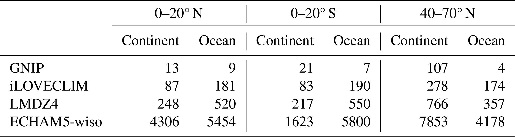
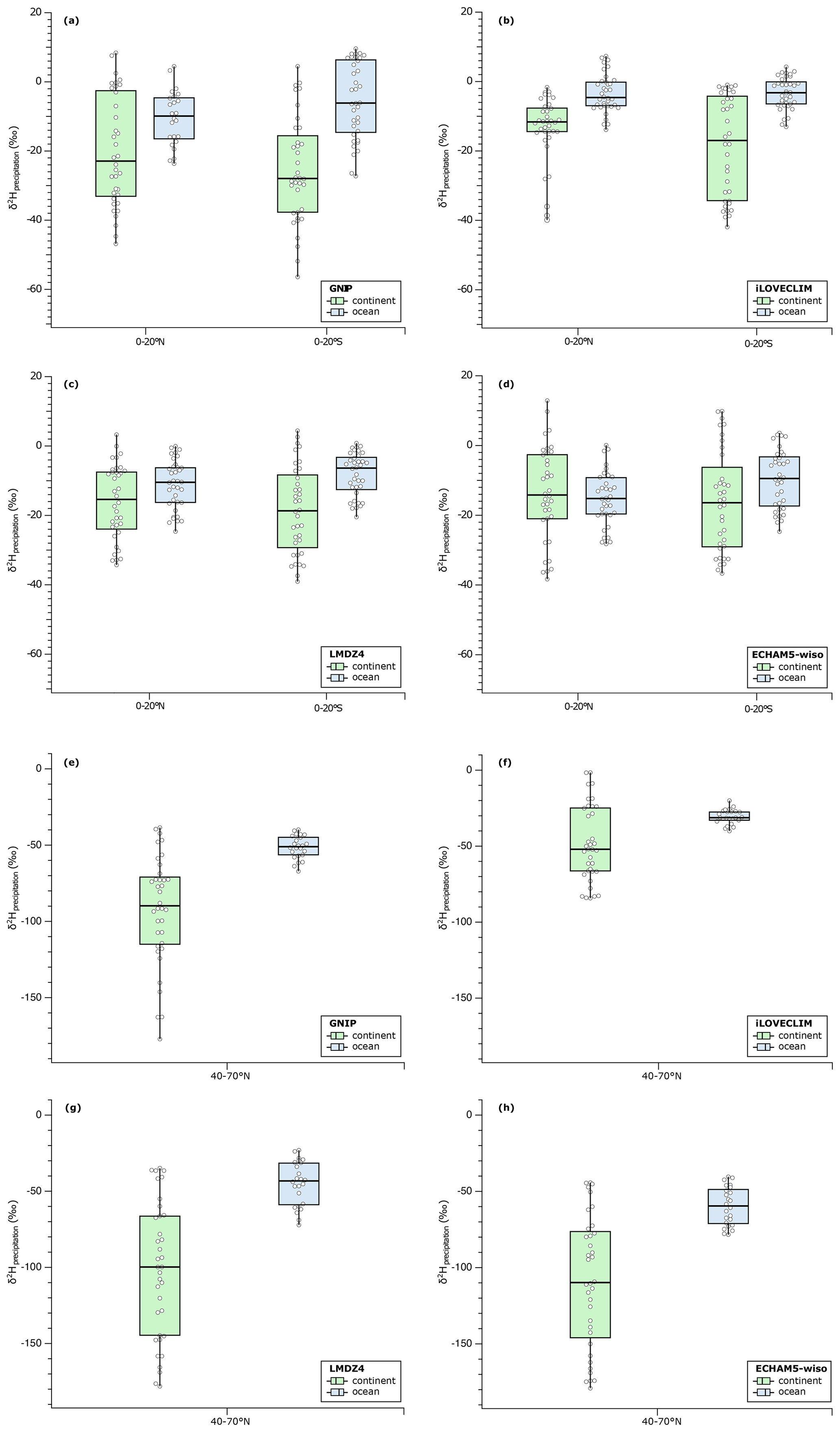
Figure 11 Boxplots of the δ²H_{precipitation} over the continents (in green) and oceans (in blue). Panels (a) to (d) present values between 0–20° N and 0–20° S for (a) GNIP data, (b) iLOVECLIM, (c) LMDZ4 and (d) ECHAM5-wiso. Panels (e) to (h) present values between 40–70° N for (e) GNIP data, (f) iLOVECLIM, (g) LMDZ4 and (h) ECHAM5-wiso. The horizontal line in the box plots corresponds to the median value.

3.3 Isotopes in ocean water

3.3.1 Surface seawater

The hydrogen isotopic ratio has been modelled in the oceanic component for the seawater. iLOVECLIM models annual-mean surface δ²H_seawater with low negative values in the Arctic Ocean that are too high compared to observations at high latitudes (Fig. 12a). This is clearly visible in the zonal distribution (Fig. 13a – with a similar methodology to Fig. 2 to take the model outputs that co-locate with the measurements and the use of a polynomial regression curve) where the δ²H_seawater trend in iLOVECLIM has too-high values for high latitudes compared to the observations and MPI-ESM-wiso. The δ²H_seawater in the Atlantic Ocean is well reproduced in the model with high values close to the tropics and the Equator and lower values in the northern and southern parts of the ocean even if the modelled values are slightly different from the observation in the northern Atlantic (Fig. 12a). The Mediterranean Sea presents good agreement with the observation with high δ²H_seawater values. The δ²H_seawater pattern in the Pacific and Austral oceans is also similar to the observations. However, the western part of the Indian Ocean and Arabian Sea presents lower values of ∼ 10 ‰ in comparison to the GISS data (Fig. 12a). This could be explained by a model bias toward higher precipitations and reduced salinity in this area. Both the iLOVECLIM and the MPI-ESM-wiso models reproduce the zonal distribution from 50° S to 20° N in comparison to the observations. They do however present differences, with a generally lower modelled δ²H_seawater value in comparison to the data and less variability in iLOVECLIM compared to MPI-ESM-wiso (Fig. 13a).

The annual-mean surface d-excess in the different oceanic basins is also presented in Fig. 12b with the measurements for comparison. The overall pattern of d-excess is similar to the one of the δ²H_seawater, with high positive values in the Arctic Ocean and lower values in the Atlantic, Pacific, Indian and Austral oceans. The modelled d-excess values from −2 ‰ to 0 ‰ in the Atlantic and Pacific oceans match the observations, with a gradient from low to high values from the low to high latitudes (Figs. 12b and 13b). The western part of the Indian Ocean and the Arabian Sea again presents values that are different from the observations. The model calculates a d-excess of ∼ 2 ‰ in the western Indian ocean, whereas the data have smaller values. The modelled d-excess even goes up to 14 ‰ in the Arabian Sea due to precipitation and the humidity effect. Even if a small number of data points exist in the Polar Ocean above 60° N (only a few measurements in the Atlantic sector), the model reproduces a too-high d-excess value in comparison to the observations, which could be explained by the absence of sea ice in this simulation. Indeed, Werner et al. (2016) have shown that fractionation happens during sea ice formation, leading to depletion of the liquid surface water isotopic composition of several per mil. iLOVECLIM also does not include river discharges that are at the origin of low isotopic values and could allow for lower d-excess than in our simulation. However, the iLOVECLIM model presents closer agreement with the measurements from the mid-latitudes to the Equator than the MPI-ESM-wiso model (Fig. 13b).

As for ¹⁷O-excess, modelled values are very low in the entire Arctic Ocean, Arabian Sea, Mediterranean Sea and along the coast of eastern and western Africa (Fig. 12c). Apart from the northern part that has negative values similar to the Arctic Ocean, the Atlantic Ocean presents relatively small ¹⁷O-excess variations and matches the data with values between 0 and 50 per meg. The Pacific and Indian oceans have higher ¹⁷O-excess values of up to 200 per meg, which is higher than observations. However, the uncertainties associated with the model and the lack of data do not allow for a good model–data evaluation for this proxy.

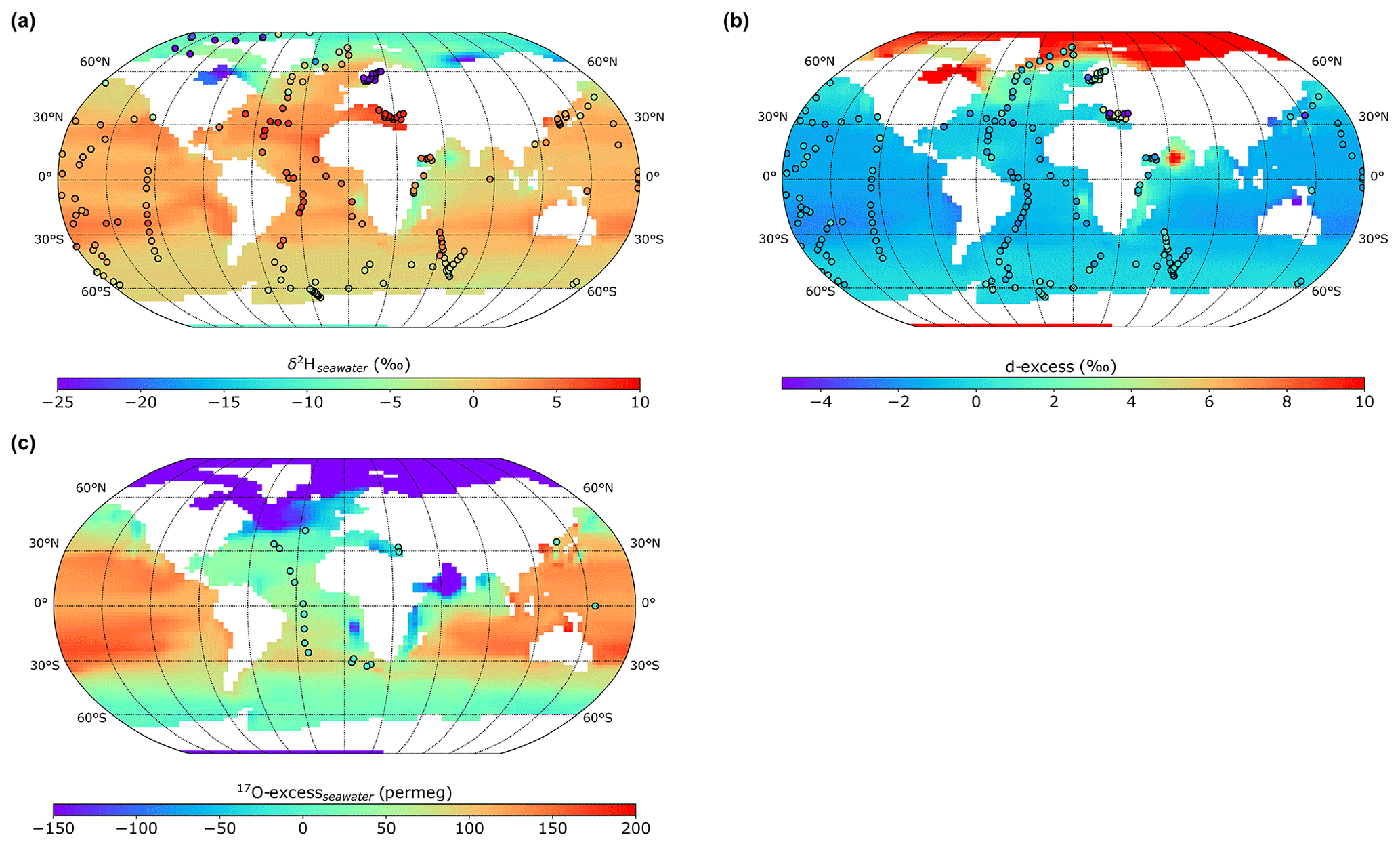
Figure 12 Model–data comparison of the annual-mean isotopic distribution in the ocean. (a) δ²H of ocean surface water, (b) d-excess of ocean surface water and (c) ¹⁷O-excess of ocean surface water in iLOVECLIM. The model results are compared to measurements (in circles).

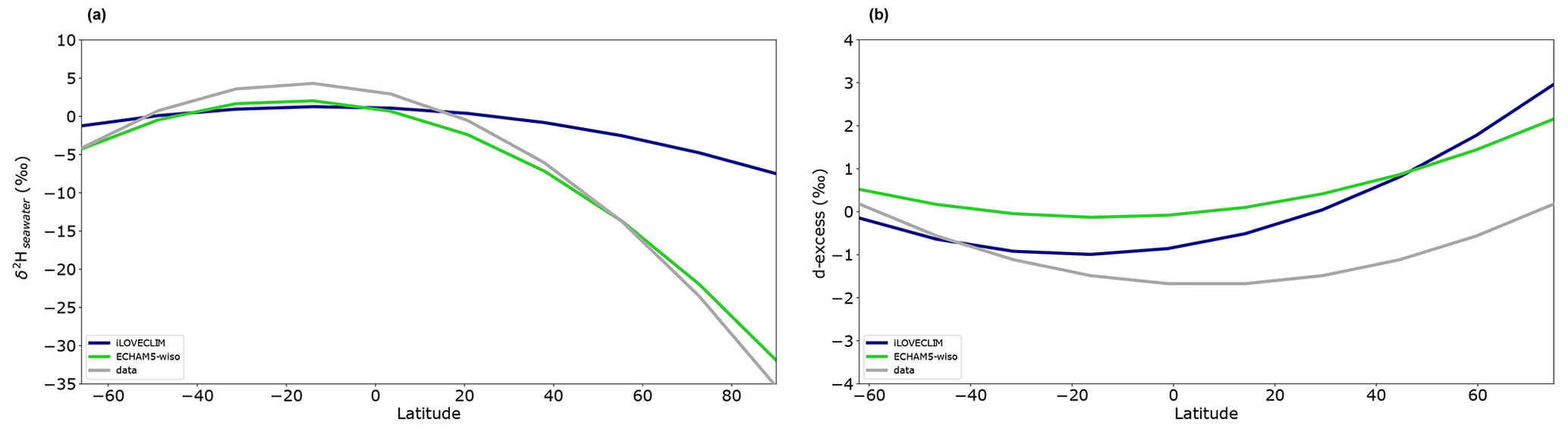
Figure 13 Multi-model zonal comparison of (a) δ²H of ocean surface water and (b) d-excess of ocean surface water. The model results (in colour) are compared to observations (in grey). The different lines are polynomial regression curves for the model results that co-locate with the observations.

3.3.2 Vertical profiles

The model–data comparison of δ²H and d-excess of seawater can be realized over the entire water column with a cross section in the Atlantic Ocean. We find general good agreement between the GISS observations and the model from the surface to the bottom with the imprint of the different water masses on the simulated δ²H (Fig. 14a). The strongest δ²H enrichment is observed in the upper Atlantic (above 700 m) between 30° S and 45° N with a maximum around 20° N with 4.2 ‰. However, there are some differences in the surface water with δ²H values that are lower than the observations by several per mil. Below 700 m, the North Atlantic Deep Water (NADW) has lower δ²H values, between 1.8 ‰ and up to 0 ‰ at the bottom of the ocean where the water mixes with the Antarctic Bottom Water (AABW) coming from the south with low values (Fig. 14a). In the Southern Ocean, around 1000 m depth, the Antarctic Intermediate Water (AAIW) flows to the north with negative low δ²H values.

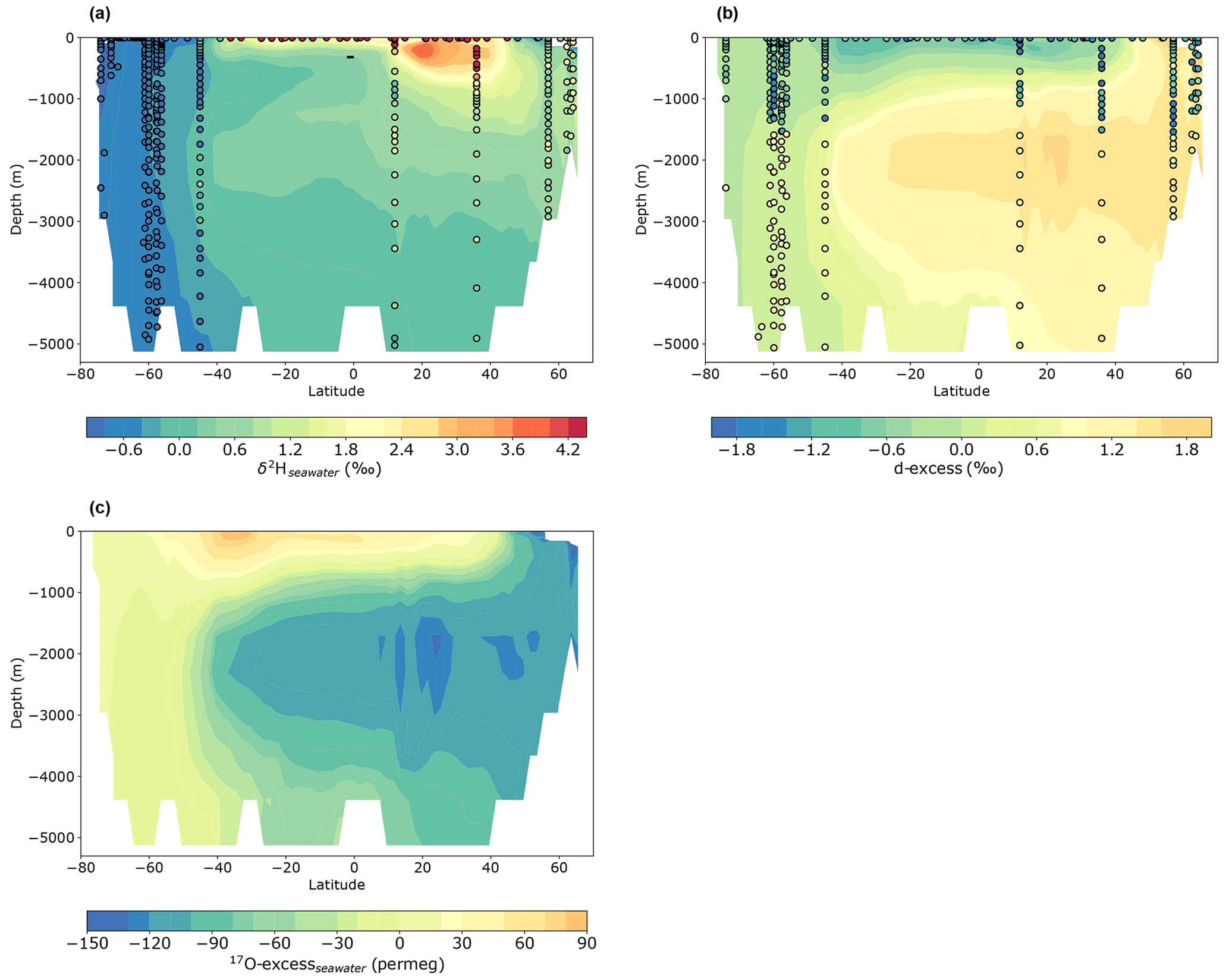
Figure 14 Atlantic zonal mean in iLOVECLIM of (a) δ²H of seawater, (b) d-excess of seawater and (c) ¹⁷O-excess of seawater compared to observations (in circles).

The oceanic d-excess and ¹⁷O-excess show a less prominent influence of the main water masses. Above 1000 m, the d-excess goes from 40° S to 40° N with low negative values (Fig. 14b) and positive values for ¹⁷O-excess (Fig. 14c). Below 1000 m and from 40° S to the north, the NADW d-excess values are higher with a maximum of 2 ‰ around 25° N and 2000 m depth. On the other hand, ¹⁷O-excess values are lower than at the surface, with minimum values at the same latitude and depth as the d-excess minimum. The comparison with the δ²H and d-excess observations shows that the model reproduces the low surface values and the high d-excess values below 1800 m even if the latitudinal gradient is more pronounced in the model than in the data. The depth interval from 500 to 1800 m presents disagreement between the modelled d-excess and the observation values that are consistently lower than in the model (Fig. 14b). This is especially the case for high latitudes of the Northern Hemisphere where the difference between the model and the data can reach 2 ‰ to 3 ‰. Since no ¹⁷O-excess observations exist at depths, we refrain from any further evaluation of the modelled values.

4 Conclusions

In this study, we presented the implementation of the ¹H²H¹⁶O and ¹H₂¹⁷O isotopologues in the intermediate-complexity coupled climate model iLOVECLIM. Based on the existing δ¹⁸O water isotopic module and this new extension, we modelled the d-excess and ¹⁷O-excess variations to have a general overview of the water isotopes. We evaluated the model isotopic ratio under preindustrial conditions for both the atmosphere and the ocean components based on a long equilibrium simulation. For the atmospheric part, we found good agreement between the model, the observations and several GCMs, with a reasonable simulation of the latitudinal gradient (considering the intrinsic biases of iLOVECLIM that could lead to local inconsistencies). The modelled δ²H and δ¹⁸O fit with the global meteorological water line, and the main isotopic effect, i.e. the amount effect, temperature effect and continental effect, are well reproduced in the model. The d-excess distribution for the atmosphere is also correctly modelled at global scale in comparison to the observations and several GCMs. However, the isotopic ratios of oxygen and hydrogen over Antarctica present differences of several per mil in comparison to the data because of the complexity of the local processes at play that are simplified in the model. At present, our model–data comparison suggests that iLOVECLIM does not correctly reproduce the ¹⁷O-excess, with an excessive dispersion of the values. Modelling the ¹⁷O-excess has to be improved in the future versions of the isotope-enabled models. New measurements are also needed with a reduction in their associated uncertainties. For the ocean, we reproduced with good agreement the modelled surface δ²H and d-excess in comparison to the existing data, except for some parts of the Arctic region and local areas in the Indian Ocean. This good agreement is conserved over the entire water column in the Atlantic Ocean, with similar δ²H values and distribution between the model and the data, influenced by the main water masses.

Given the computing resources needed to run coupled climate models, applying intermediate-complexity coupled climate models with water isotopes like iLOVECLIM to future long-term palaeoclimate perspectives appears to be very promising. Palaeoclimate simulations during the Holocene, the Last Glacial Maximum or transient glacial/interglacial periods are the next logical step to compare model results against past isotopic ratio records. New proxies that depend on the water isotopes can also be implemented in the model, like the leaf wax isotopic ratio, in order to quantify the influence of the respective factors (e.g. precipitation, vegetation, humidity) that control its variations.

Appendix A: δ¹⁷O isotopic composition

The latitudinal gradient and the global distribution of the modelled δ¹⁷O are similar to the ones of the δ¹⁸O with low values from the Equator to the poles (Fig. A1a). Similarly, the values over land are lower than those over the ocean. In comparison to the available data (including new data from Terzer-Wassmuth et al., 2023), iLOVECLIM models higher values of several per mil in central Europe and Canada and lower values in Africa. Agreements are observed between the model and the data in eastern Asia, western Europe and North America. The discrepancies can be explained by the fact that most of the data are punctual and reflect seasonal conditions, whereas the model outputs are annual-mean δ¹⁷O values.

δ¹⁷O of seawater in iLOVECLIM shows values close to 0 over the Atlantic, Pacific, Indian and Southern oceans, which is consistent with the observations (Fig. A1b). The amplitude of variation is small and around 1 ‰. The coast of eastern Africa and the Arabian Sea present lower values, as well as the northern part of the Atlantic Ocean and the Arctic Sea with negative values of up to −4 ‰.

Figure A2 presents the relationship between the modelled and measured δ¹⁷O_{precipitation} (excluding values in Antarctica). Most of the values modelled in iLOVECLIM are grouped around high isotopic values, but the correlation remains low. The model results are statistically significant with a p value of 0.007 (<0.05). In comparison to LMDZ4, which is currently the only GCM to include the ¹⁷O (Risi et al., 2013), iLOVECLIM results are in good agreement with most of the values between 0 ‰ and −7 ‰, leading to a similar linear trend between the model and the data. Towards negative values, LMDZ4 gets closer to the 1:1 line than iLOVECLIM. However, considering the large confidence intervals for both model results, the modelled δ¹⁷O_{precipitation} in iLOVECLIM could be in agreement with the values obtained in LMDZ4. The differences between the model results and the data could be related to the fact that most of the data are punctual and reflect seasonal conditions, whereas the model outputs are annual-mean δ¹⁷O values and have a low number of measurements to be compared with.

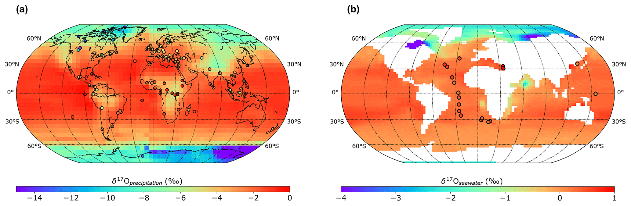
Figure A1 Mean annual spatial distribution of the iLOVECLIM-modelled (a) δ¹⁷O_{precipitation} and (b) δ¹⁷O of the ocean surface. Model results are compared to observations (in circles).

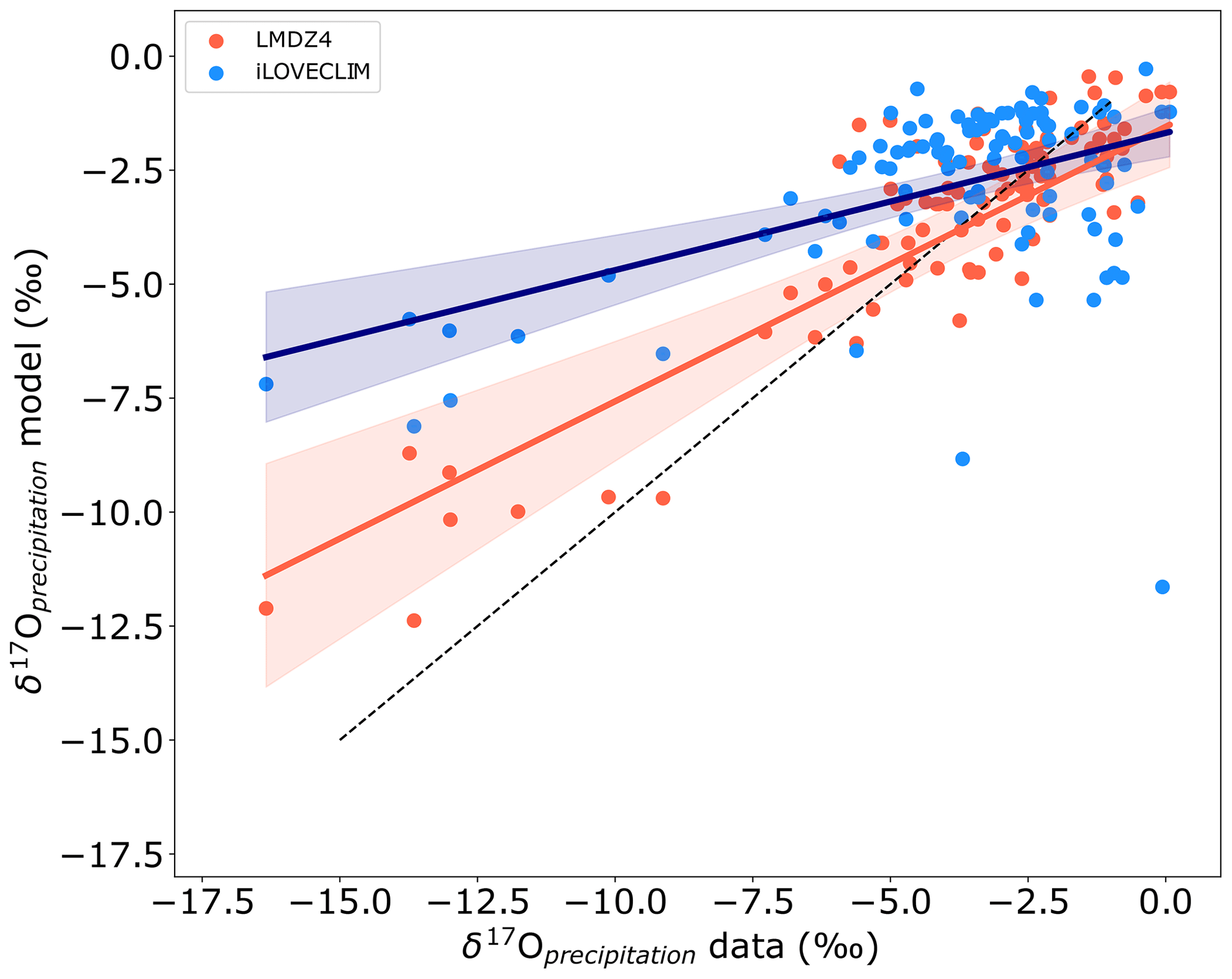
Figure A2 Model–data relationship for the δ¹⁷O_{precipitation} without Antarctic values for the iLOVECLIM (blue) and LMDZ4 (red) models. The regression curves between the model and data are presented in dark blue for iLOVECLIM and red for LMDZ4 with the confidence bands. The 1:1 line is shown with the dashed black line.

Appendix B: Seasonal variations

We investigate the amount effect by looking at seasonal variations in the precipitation and isotopic ratio. For an easier comparison in the main text, we normalized the values because the seasonal evolution in the model is not expected to perfectly reflect the measurements. We present here in Fig. B1 the raw values. The seasonal variation in the precipitation and δ²H_{precipitation} is the same as that presented in Sect. 3.2.1 with the normalized values (Fig. 8). The lead and lag of the iLOVECLIM and LDMZ4 models to the data are also conserved. However, differences are observed in the amplitude, mostly for the isotopic ratio, with lower values of up to 15 ‰ in summer for the northern tropics between the data and the models. The same difference in absolute values between the observation and the models is observed in the southern tropics.

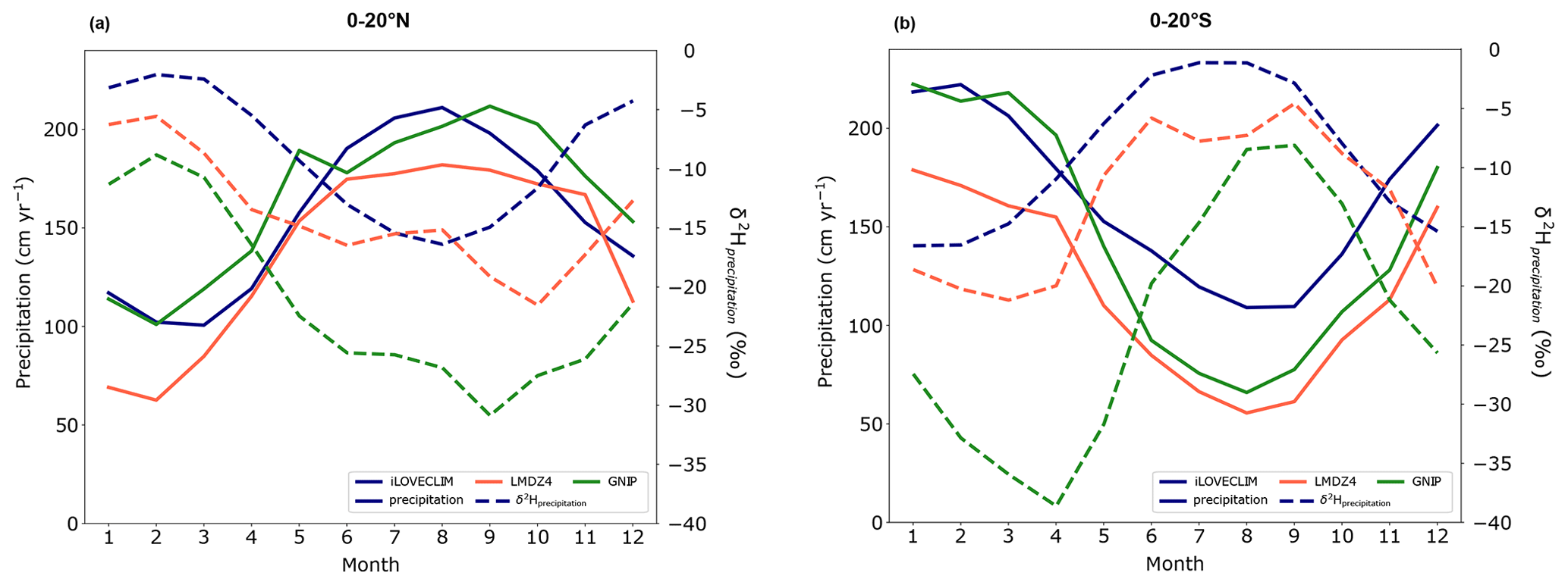
Figure B1 Seasonal variations in the mean precipitation and δ²H_{precipitation} in the tropics, from 0–20° N (a) and 0–20° S (b). The solid lines represent the precipitation and the dashed lines the δ²H_{precipitation}. The blue curve presents the iLOVECLIM raw values, the red curve is for LMDZ4 and the green curve corresponds to the GNIP data.