the Creative Commons Attribution 4.0 License.
the Creative Commons Attribution 4.0 License.
 | 13 Mar 2024
A generic algorithm to automatically classify urban fabric according to the local climate zone system: implementation in GeoClimate 0.0.1 and application to French cities
Erwan Bocher
Matthieu Gousseff
François Leconte
Elisabeth Le Saux Wiederhold
Geographical features may have a considerable effect on local climate. The local climate zone (LCZ) system proposed by Stewart and Oke (2012) is nowadays seen as a standard approach for classifying any zone according to a set of urban canopy parameters. While many methods already exist to map the LCZ, only few tools are openly and freely available. This paper presents the algorithm implemented in the GeoClimate software to identify the LCZ of any place in the world based on vector data. Six types of information are needed as input: the building footprint, road and rail networks, water, vegetation, and impervious surfaces. First, the territory is partitioned into reference spatial units (RSUs) using the road and rail network, as well as the boundaries of large vegetation and water patches. Then 14 urban canopy parameters are calculated for each RSU. Their values are used to classify each unit to a given LCZ type according to a set of rules. GeoClimate can automatically prepare the inputs and calculate the LCZ for two datasets, namely OpenStreetMap (OSM, available worldwide) and the BD TOPO® v2.2 (BDT, a French dataset produced by the national mapping agency). The LCZ are calculated for 22 French communes using these two datasets in order to evaluate the effect of the dataset on the results. About 55 % of all areas have obtained the same LCZ type, with large differences when differentiating this result by city (from 30 % to 82 %). The agreement is good for large patches of forest and water, as well as for compact mid-rise and open low-rise LCZ types. It is lower for open mid-rise and open high-rise, mainly due to the height underestimation of OSM buildings located in open areas. Through its simplicity of use, GeoClimate has great potential for new collaboration in the LCZ field. The software (and its source code) used to produce the LCZ data is freely available at https://doi.org/10.5281/zenodo.6372337 (Bocher et al., 2022); the scripts and data used for the purpose of this article can be freely accessed at https://doi.org/10.5281/zenodo.7687911 (Bernard et al., 2023) and are based on the R package available at https://doi.org/10.5281/zenodo.7646866 (Gousseff, 2023).
- Article
(6508 KB) - Full-text XML
- BibTeX
- EndNote


In its Sixth Assessment Report, the Intergovernmental Panel on Climate Change (IPCC) underlines that cities demonstrate a two-way interaction with the climate system (IPCC, 2007). While they impact the climate locally (modification of the energy and mass balances) and globally (greenhouse gas, GHG, and emissions), urban areas are also vulnerable to meteorological hazards (Baklanov et al., 2020). Cities are very likely to face extreme climate events such as heatwaves more frequently in the coming decades (IPCC, 2007). The United Nations (UN) has identified urban resilience as a key challenge via its Sustainable Development Goals (SDGs) (i.e., SDG 11, sustainable cities and communities) (Grimmond et al., 2020). Climate change attenuation and adaptation strategies are currently being designed and implemented in cities. The efficiency of these strategies relies on our knowledge of the urban environment and our understanding of the urban climate.
The description of the urban fabric is essential for urban climate research, both for observation and modeling purposes. Regarding observation, measurements of physical variables (such as air temperature, surface temperature, and relative humidity) are analyzed relative to local-scale urban features (e.g., mean size of street canyons) and micro-scale urban features (e.g., distance between the measurement point and a given wall), while models require information about building morphology, land use, materials, and anthropogenic fluxes as input data. However, urban data collection has been identified as a challenging task (Masson et al., 2020).
In this context, many classification systems have been promoted to standardize the study of urban climate. In the last decade, the local climate zone (LCZ) classification (Stewart and Oke, 2012) has encountered a growing interest amongst urban climate researchers. A local climate zone is an area that demonstrates particular urban characteristics in terms of morphology, land use, materials, and anthropogenic heat release, leading to a distinct thermal behavior under given weather conditions. Its size is approximately 400–1000 m wide. The LCZ classification system is organized into 17 LCZ types (10 urbanized and 7 non-urbanized). It requires the calculation of 10 urban canopy parameters (UCPs): sky view factor (SVF); aspect ratio; height of roughness element; terrain roughness class; surface fractions (built, impervious, and pervious); surface admittance; surface albedo; and anthropogenic heat output. Each LCZ type is associated with particular values of these 10 UCPs (e.g., LCZ 1, called compact high-rise, has a sky view factor between 0.2 and 0.4, an aspect ratio higher than 2, and a height or roughness class equal to 8.).
The construction of LCZ maps for an area of interest is very time-consuming if not automated. In their review, Quan and Bansal (2021) have identified two main research streams to build LCZ maps automatically. The first stream uses remote sensing images as main input data. A prominent initiative of this remote sensing approach is the World Urban Database and Access Portal Tools (WUDAPT) (Ching et al., 2018). Within this project, a LCZ-generator tool has been released (Demuzere et al., 2021). It is based on a random forest model trained with areas that have been classified by experts to a given LCZ type. The corresponding workflow has been applied to several continents (Demuzere et al., 2019, 2020). The second stream involves detailed geographical information (often presented as vector data) processed by a geographic information system (GIS). It is organized into six main steps (Quan and Bansal, 2021):
-
collection of geographical data;
-
partitioning of the territory using a reference spatial unit (RSU, called basic spatial units by Quan and Bansal, 2021), defined as the smallest spatial unit where calculations are performed;
-
calculation of several UCPs within each RSU;
-
assignation of a LCZ type to each RSU based on UCP values;
-
post-processing, e.g., merging adjacent RSUs for simplification and sizing purpose; and
-
evaluation of the LCZ map.
In the first stream, experts may not use the UCP values to attribute a LCZ type to a given area, thus leading to subjective decision while an objective LCZ referential has been proposed. However, due to the growing accessibility to high-quality satellite images, it is applicable to most countries in the world. The second stream is spatially limited to the territory where a specific geographical dataset is available (often a city or a country). Its main advantage is that the UCPs used in the LCZ reference list are often calculated, inducing a potentially more objective method than the first stream. Another advantage is that geographical information can be crowd-sourced, which is probably less energy-greedy than the use of, for instance, aerial photography.
For each of the six steps of this second stream, Quan and Bansal (2021) have observed a great diversity of methods. In step 1, the data collection concerns mostly vector data, such as the building footprint, building height, or road cover. However, to determine surface fractions, satellite or airborne images are often used. The definition of the RSU (step 2) varies significantly amongst studies. It can be estimated by local knowledge (Leconte et al., 2015). It can also corresponds to lot area polygons (i.e., influential area surrounding each building) (Skarbit et al., 2017); urban blocks (i.e., urban unit naturally bounded by streets) (Quan et al., 2017); or regular grids (Geletič et al., 2016). The vast majority of the methods does not calculate all 10 UCPs included in the LCZ framework (step 3). The most calculated UCPs are the surface fractions and the height of roughness elements, followed by the sky view factor and the aspect ratio. However, additional UCPs are often proposed, such as building density, population density, areal number density, and additional surface fractions. Concerning step 4, previous studies adopted mainly three workflow types to assign a LCZ type to a given RSU: the standard-, modified-, and fuzzy-rule-based approaches. The standard-rule-based approach associates a RSU with a given LCZ type only if all UCP values fall within the UCP value ranges of the LCZ type (the other RSUs are set as unclassified). The modified standard-rule-based approach often uses fewer than 10 UCPs, adds new UCPs, and proposes new rules for the LCZ-type assignment (such as decision trees). The fuzzy-rule-based approach calculates a degree of membership based on UCP values. For a given RSU, it selects the LCZ type with the highest degree of membership. Step 5 consists of merging the RSUs to simplify overcomplicated LCZ maps and to meet the size requirement of the LCZ scheme (LCZ larger than 400 m). This stage also aims to smooth LCZ boundaries and partially reduce the number of unclassified areas. Finally, LCZ maps are sometimes evaluated against expert knowledge, temperature measurements, or other LCZ maps provided by remote sensing methods (step 6).
LCZ map workflows usually face two key issues, namely a lack of input data and a partially described methodology (Quan and Bansal, 2021). This study presents a new automated workflow for LCZ map construction that addresses these issues by the following contributions.
-
The workflow has been designed to be generic; it accepts all datasets as soon as the input data are structured, following a well-described guideline (Bocher et al., 2021), and can be run with any type of RSU. The GeoClimate workflow is already designed to work with two input data types, namely BD TOPO® v2.2 and OpenStreetMap. The first is a French government dataset, while the latter is an open-source project that provides geographical information worldwide and therefore tackles the data-scarcity issue.
-
The workflow, described in detail within this article, is integrated in GeoClimate, a free and open-source software, and thus the code is fully open-source and available online (https://github.com/orbisgis/geoclimate/wiki, last access: 7 February 2023) (Bocher et al., 2021).
This article presents the GeoClimate methodology to produce LCZ maps. Additionally, it is applied to 22 French cities using the worldwide available OpenStreetMap data and compared to the results of using the same method with the French reference dataset BD TOPO® v2.2. This comparison is useful for observing the respective advantages and shortcomings of each dataset and how they could be combined together for application to the French territory.
2.1 GeoClimate library
GeoClimate is a free and open source toolbox developed in Groovy language that allows geographical indicators calculation from vector-based data. It consists of a preprocessing workflow where input data are processed to following a generic data structure, according to well-described guidelines (Bocher et al., 2021), and in a processing workflow where all indicators are calculated based on this generic input data.
The preprocessing workflow of the GeoClimate version (0.0.1) currently supports two data source providers: the BD TOPO® database (version 2.2, hereafter BDT) produced by the French national mapping agency (IGNF, https://geoservices.ign.fr/, last access: 7 February 2023) and the community database OpenStreetMap (hereafter OSM, https://www.openstreetmap.org, last access: 7 February 2023). Once the input data source is selected, GeoClimate applies a set of rules to extract and format the required spatial descriptors and then build six GIS layers, namely the building footprint, road and rail network, water, vegetation, and impervious surfaces. GeoClimate performs all analysis on an extended zone (1000 m larger than the original study area), and then the results are cropped to the initial zone of interest (limiting the edge effects at the boundary of the study area). Each layer follows a set of specifications to ensure the completeness and logical consistency of the input data and avoid potential geometry inconsistencies. For example, only a single geometry is allowed for the description of a feature (multipolygon or multipolyline are exploded), the values used to qualify a building type or a vegetation type are restricted to the ones available in a dictionary provided by GeoClimate, and some numeric attributes such as the width of a road are bounded by extreme values. Any data source can then be connected to the GeoClimate LCZ processing chain (and thus for any place in the world), as long as the connection to the GeoClimate input data model is performed respecting the set of specifications described in Bocher et al. (2021).
The next step concerns the construction of two new spatial units: building blocks and RSU.
-
A building block is defined as an aggregation of buildings that are in contact.
-
A RSU (reference spatial unit) is generated according to several geographic features which could have an impact on environmental and climate effects and which structure the study area, including the road and rail networks, as well as the vegetation and water surfaces. The construction of the RSU is a key process in GeoClimate. First, a planar graph is built using all input geometries. The planar graph is then traversed to generate new polygons. Only two-dimensional elements are considered for partitioning; therefore, underground (such as tunnels) or overground (such as bridges) elements are excluded from the input. Water and vegetation surfaces are also excluded from the input data when they are smaller than a given threshold set by default to 2500 m2 for water and 10 000 m2 for vegetation. This behavior is visible in Fig. 1. At the northern part of the river, many small vegetation patches are not considered for RSU creation, while they are when they get bigger than 10 000 m2 (along the river on its southern part or on the western part of the area).
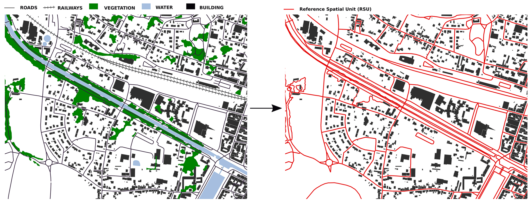
Figure 1Illustration of the method to produce the reference spatial units using BDT data.
The geographical indicators are then computed using the seven GIS layers to characterize the geometric properties and the location of the spatial features regarding the following three scales: buildings, building blocks, and RSUs. At the building scale, GeoClimate measures the distance to the nearest road and the number of building neighbor, area, and shape indices (concavity and compactness). At the building block scale, the volume, main orientation, and total areas of the courtyard are computed, while at the RSU scale, the building and building block indicators are aggregated (average number of levels per building and density of building floor areas) plus land type fractions and specific climate-oriented indicators such as aspect ratio and mean sky view factor.
At the end, more than 100 indicators are available. Those indicators are used to describe the land fabric, to feed parametric climate models, such as the Town Energy Balance (TEB) or the Weather Research and Forecasting (WRF) models, and to perform classifications such as the local climate zones.
2.2 Indicators used
The 14 indicators needed for the LCZ classification procedure are described in Table . Note that the land cover fraction used in this work is calculated considering that high vegetation may be above any other land cover (including buildings). Thus, if the high vegetation is superimposed on another land cover, then the sum of all land cover may be higher than 1.
Bernard et al., 2018Hanna and Britter (2010)Table 1Description of the calculation method for each indicator used.
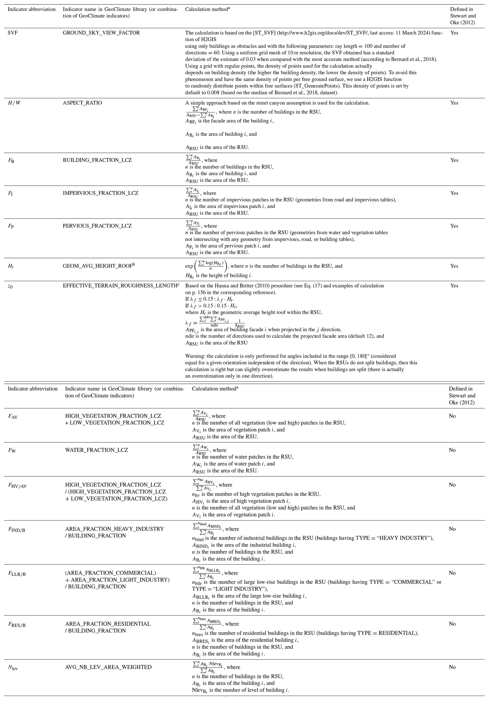
a This calculation is generic for any dataset, since GeoClimate is based on a generic model described by Bocher et al. (2021). b Stewart and Oke (2012) calls this the “height of roughness elements” and also consider the tree height in the calculation. c In Stewart and Oke (2012), terrain roughness classes are actually used, which are defined according to roughness length ranges of values. We prefer to keep the length, which is continuous information (whereas the class would be a categorical variable).
2.3 Algorithm
In the GeoClimate code, the LCZ algorithm that assigns a LCZ to each RSU is called identifyLczType. It can work for any RSU definition, as long as all necessary indicators have been previously calculated for these units. The method, based on the Stewart and Oke (2012) approach, is illustrated in Fig. 2.
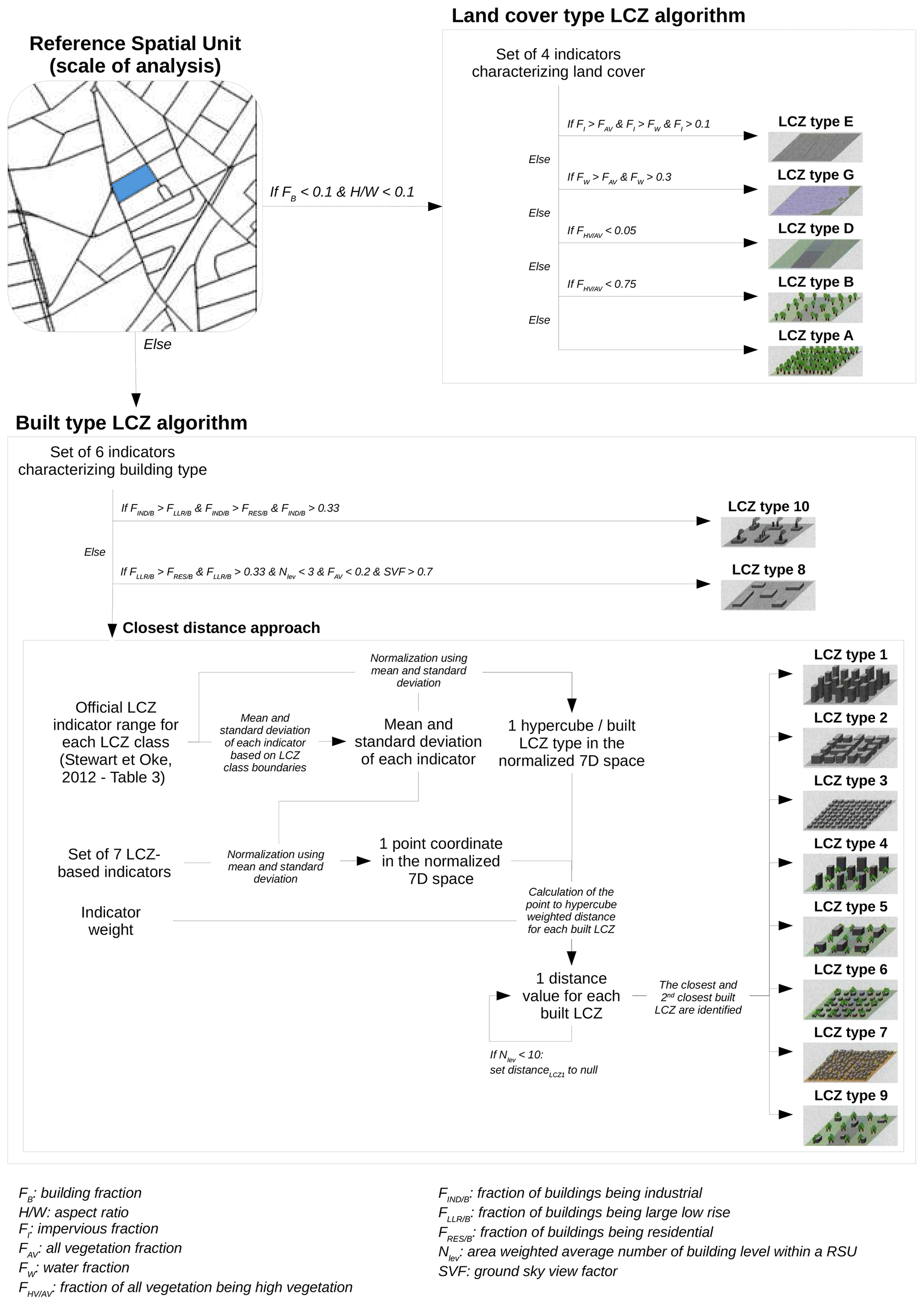
A RSU is treated differently regarding the number and the size of the buildings it contains. If the building fraction and the aspect ratio are both lower than 0.1, then the RSU is considered only as a land cover type, and its LCZ will be affected using the land-cover-type LCZ algorithm. Otherwise, the built-type LCZ algorithm will be used. The threshold of 0.1 is set according to Stewart and Oke (2012); the building fraction and aspect ratio are higher than 0.1 for all LCZ built types, while they are lower for all LCZ land cover types (if trees are excluded from the aspect ratio calculation, which applies in our case).
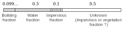
The land-cover-type algorithm currently works for five of the seven LCZ land cover types: LCZ types A, B, and D (respectively, dense trees, scattered trees, and low plants); LCZ type E (bare rock or paved); and LCZ type G (water). LCZ type F (bare soil or sand) and LCZ type C (bush and scrubs) cannot be identified, since we currently consider only five land cover types, i.e., buildings, impervious, water, low vegetation, and high vegetation. We first consider that our raw data are continuous anywhere on the planet; thus, any piece of land should be covered by one of the five selected land cover types. This assumption can induce some errors in cases where there is missing information in the data source. After considering the building fraction (which is lower than 0.1 for non-urbanized LCZ types), if the impervious fraction is higher than the water fraction and higher than the vegetation fraction (low and high), then the RSU can be set to LCZ type E (impervious), since impervious areas correspond to the major fraction. In reality, the sum of our land fractions rarely reaches 100 %. Depending on the data we use, we may have non-identified areas. The position and the size of buildings, roads (at least the center line), and water are often accurately known. However, this is not the case for vegetation (especially in urban private lands) and impervious areas (such as a sidewalks and parking lots). Thus, a land cover fraction should be higher than a given threshold in addition to representing the major fraction of a RSU. The higher the probability that a given land cover is missing from the data, the lower the corresponding threshold. Based on empirical observations using OSM and BDT, we set these thresholds to 0, 0.1, and 0.3, respectively, for vegetation, impervious, and water. Hence, a RSU must satisfy the following condition: having a vegetation fraction higher than 0.3 to be a water LCZ, an impervious fraction higher than 0.1 to be a paved LCZ, and a vegetation fraction higher than 0. Results from simple examples are presented in Fig. 3. If impervious and water fractions are below their threshold (respectively, 0.1 and 0.3), then the land cover type is set to vegetation. Whenever impervious or water fractions exceed their threshold, they should also be larger than any other land cover fractions. If the land cover is vegetation, then the LCZ type is set according to the high vegetation fraction for the vegetation (low and high) fraction ratio. The threshold values to distinguish low plants from scattered trees and scattered trees from dense trees have been roughly set to 0.05 and 0.75; these values were chosen arbitrarily from the drawing of each class and empirical observations using our data.
The built-type algorithm works for all LCZ built types. It is mainly based on a closest-distance approach (called the fuzzy-rule-based approach in Quan and Bansal, 2021). Stewart and Oke (2012) proposed a set of seven UCPs to characterize the morphology and the land cover properties of a given area. In Table 3 of their work, they set, for each of the LCZ types, a range of possible values taken by each of these UCPs. In a formal approach, a LCZ type is defined as an hypercube in a seven-dimensional space. In this space, a given RSU is defined by a point, and its coordinates are the value of the seven UCPs. Then, the closest-distance approach consists of identifying the LCZ-type hypercube that is closest to our RSU point. Note that the distance is clearly influenced by the dimension with the largest variability; the building height, which can vary from zero (no building) to several hundred meters for the highest buildings, will have much more impact on the distance than the building fraction, which is included in a [0, 1] range. Thus, each dimension is normalized using the mean and the standard deviation of all LCZ-type boundary values (note that we have replaced the initial terrain roughness class indicator with the more continuous information of the effective terrain roughness length using the conversion table in Davenport et al., 2000). However, we leave the opportunity to give more importance to some of the UCPs in the form of adding a given weight to each dimension. This can be useful for several reasons:
-
the data used as input may not represent the reality well; thus, we may decrease the weight of all impacted axes (e.g., pervious fraction if the vegetation is rarely identified);
-
the method used to calculate some UCPs might not be in total agreement with the Stewart and Oke (2012) definition (SVF does not take into account vegetation nor elevation), which is a reason to decrease its corresponding weight; and
-
the user may simply think that the seven UCPs should not have equal weight in the classification.
Actually, three LCZ built types have a specific behavior.
-
In LCZ 1 (compact high-rise), the closest-distance approach is used, but the distance of a RSU to the LCZ 1 hypercube is set to null wherever the mean number of building level in the RSU is lower than 10 (threshold set according to the Stewart, 2011, description of LCZ 1). Without this constraint, we have obtained LCZ 1 in numerous European cities in which most of the urban researchers would not set any (Demuzere et al., 2019).
-
In LCZ 10 (heavy industry), the shape and the land cover of these zones results directly from the building use. Thus we decide to exclude this LCZ type from the closest-distance approach. Instead, a RSU is set as heavy industry when its fraction of heavy industry among the buildings exceeds those of residential buildings and large low-rise buildings and when it is higher than 0.33.
-
In LCZ 8 (large low-rise), as for LCZ 10, we set a RSU as large low-rise when its building fraction exceeds that of industrial and residential and is higher than 0.33. However, even though the building use allows a simple identification of those areas, we may have a mid- or high-rise mall in our sample. Thus, the maximum average number of building levels should be lower than three, the SVF should be higher than 0.7, and the vegetation fraction lower than 0.2 (these thresholds come from Stewart and Oke, 2012, and Stewart, 2011).
At the end of the closest-distance algorithm, two LCZ types are conserved: the closest (called LCZ Primary) and the second-closest (LCZ2 Secondary). For all the RSUs set with another approach, only LCZ Primary has a value (LCZ2 Secondary is set to null).
2.4 Indicators of uncertainty
Once the LCZ type of each RSU is set, we can consider how accurate this information is. If the LCZ type has been set according to the closest-distance approach, then the distance to the closest LCZ is stored in the MIN_DISTANCE field. If the distance is 0, it means that the point is within the hypercube. Then higher this value, the worse the classification will be. However, a point may have a relatively low MIN_DISTANCE but be at an almost equal distance to several hypercubes. Then we calculate the LCZ_UNIQUENESS_VALUE defined by Eq. (1). Its value ranges between 0 and 1; the higher it is, the more relevant the LCZ type set to the RSU.
where dclosestLCZ is the distance from the RSU point to the closest LCZ hypercube, and is the distance from the RSU point to the second-closest LCZ hypercube.
In all other cases (when the LCZ type is not set using the closest-distance approach), MIN_DISTANCE and LCZ_UNIQUENESS_VALUE are set to null by default.
2.5 Sensitivity analysis: influence of the input data
The LCZ procedure proposed in GeoClimate is generic in the sense that it works with a fixed input table set. However, we want to investigate the impact of input data modification (BDT or OSM) on the resulting LCZ map. According to preliminary observations, we have identified two major differences between these data; the building height is not filled for most buildings in OSM, while land cover coverage seems better in OSM than in BDT.
Lack of building height data is a major concern for urban climate studies. For this reason, the missing heights have been estimated using a random forest method, based on geographical indicators characterizing the building environment (Bernard et al., 2022). Although the RSU mean building height could be quite far from the truth for certain areas, other indicators such as the ground sky view factor are less impacted by the quality of the building height estimation. Then we expect that the LCZ classification using these modified OSM data would lead to comparable results when using BDT data.
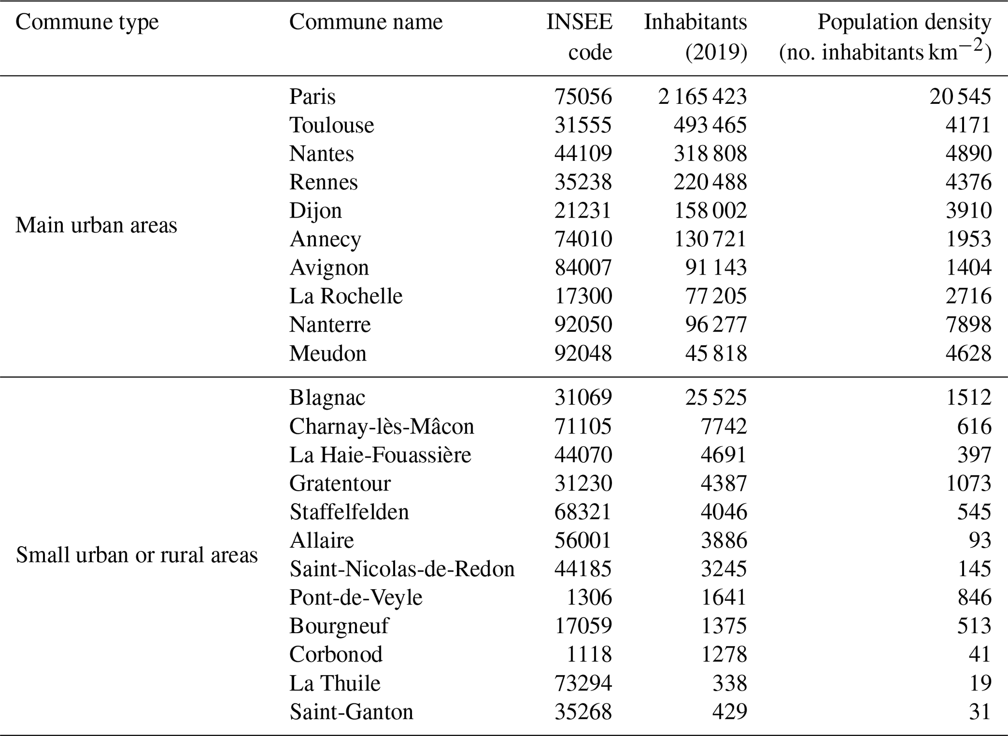
Concerning land cover coverage, we expect OSM results to have a lower fraction of undefined land (this fraction is calculated and called UNDEFINED_FRACTION for each RSU). To verify these expectations, we have run GeoClimate on the 22 French communes that have previously been used in Bernard et al. (2022). More information about these territories is given in Table 2.
Table 2Information and statistics about the communes used as study areas. Note: INSEE stands for the French National Institute of Statistics and Economic Studies (Institut national de la statistique et des études économiques).
The GeoClimate LCZ algorithm is partially based on relative weight indicators (see Sect. 2.3). Default weights have been used for each indicator, both OSM and BDT, with 4 for SVF, 3 for , 8 for FB, 0 for FI, 0 for FP, 6 for Hr, and 0.5 for z0. Those weights are only used in the closest-distance approach for LCZ built types. Two main characteristics differentiate the LCZ types, namely building capacity (mainly described by FB, SVF, and ) and building height (mainly described by Hr, , and SVF). FP and FI weights are set to zero, since they are secondary characteristics, and pervious and impervious data often lack accuracy in urban areas (this is the case for our input datasets). FB and Hr indicators are simply defined and are based on very few input variables and thus do not propagate uncertainties. However, the building height is less certain than the building footprint (especially for OSM data), thus FB has the highest weight. The SVF and have lower weights, since they do not consider all the variables they should (vegetation and terrain-level variations are excluded from the calculations). Moreover, the calculation method assumes that all LCZ built types are street canyons; thus, we set its weight slightly lower than SVF, which is calculated considering the real building setting. We may have had to decrease the Hr weight for the OSM data, but preliminary tests showed that decreasing its value down to 2 does not affect the results much.
3.1 Scale used for comparison
The spatial units generated with OSM differ from those created with BDT since the territory segmentation is performed using topographical data coming from two different sources. BDT partitioning results in about twice the number of RSU than OSM partitioning for most of the territories. Thus, the mean RSU area is more than twice as large in OSM than in BDT data (18 514 vs. 8636 m2). The median RSU area are much smaller than the mean (3013 for OSM and 1167 m2 for BDT), revealing the influence of some bigger RSU. However, the ratio between the OSM median RSU size and BDT median RSU size remains higher than 2. Three main reasons explain this observation. First, many forest patches outside city centers present in BDT do not exist in OSM. Second, some roads which are considered of secondary importance in OSM are conserved for segmentation in BDT. Third, the rules to edit data in OSM are more restrictive than BDT due to relational data model used by OSM to store and describe the geometry. In BDT, the geometries are stored in layers independently of each other (e.g., vegetation and water); consequently, there is a higher probability of finding overlaps and gaps between the layers (e.g., a surface of impervious that covers a surface of water) than in OSM. Indeed, in OSM all geometries are defined in three tables (nodes, ways, and relations); therefore, snapping between geometries is more consistent, resulting in a lower number of very small RSUs (Fig. 4). To compare the LCZ at RSU scale, a first step is then to create as many units as there are RSU intersections between the two datasets, thus leading to an increase in the small size units.
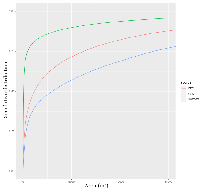
Figure 4Cumulative distribution function of RSU areas with OSM input, BDT input, and their intersection.
3.2 General agreement
For each LCZ, the areas of the geometries that received the same LCZ value using BDT or OSM data as input are summed to compute a weighted agreement per LCZ value and a general agreement for the whole commune.
A figure comparing the OSM and BDT results is automatically generated for each city using the lczexplore R package (https://github.com/MGousseff/lczexplore, last access: 7 February 2023). It contains the LCZ map created for both datasets, a bi-colored map (red and green) that shows the spatial distribution of the zones in agreement, and a confusion matrix based on percentage of area in agreement for each LCZ type. Figures 5 and 6 show a comparison of the LCZ obtained for the city of Dijon and for the rural commune of Saint-Nicolas-de-Redon, respectively. They illustrate well the main similarities and differences observed for major cities and rural territories.
Concerning Dijon, the city center (compact LCZ built types) and the urban ring (open LCZ built types) are well identified in BDT and OSM, even though the city center seems slightly bigger in OSM than in BDT. The built-up zone is visually more homogeneous in OSM than in BDT. The first reason is that the model used to predict OSM building height smooths its spatial variations (Bernard et al., 2022). The second reason is that the territory is more fragmented when using BDT compared to OSM data (the number of RSUs is 4548 and 2819, respectively, for the whole Dijon commune). In the rural areas outside the city, the LCZ vegetation type is more diverse in BDT than in OSM. However, there is a rather good spatial agreement (81 %) between zones covered by vegetation when we do not consider LCZ vegetation types (when we merge all vegetation). The agreement matrix can be used to identify the main misclassifications; for instance, 84 % of the area set to compact low-rise using BDT data is set to compact mid-rise using OSM data. However, the compact low-rise type covers a negligible fraction of the Dijon territory (0.51 %), as shown in the legend of Fig. 5 (the upper-left map).
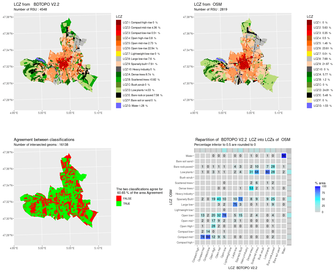
Figure 5Comparison of LCZ generated for the city of Dijon by the GeoClimate method using BDT and OSM datasets.
Concerning Saint-Nicolas-de-Redon, the observations made for Dijon remain valid; the center of the village is well identified using both OSM and BDT data. The vegetation is more heterogeneous in BDT than in OSM, resulting in a rather low agreement fraction (44 %). For such a territory with a very low LCZ built type, the vegetation type has a considerable impact, since once the vegetation is merged, the general agreement fraction is very high (94 %).
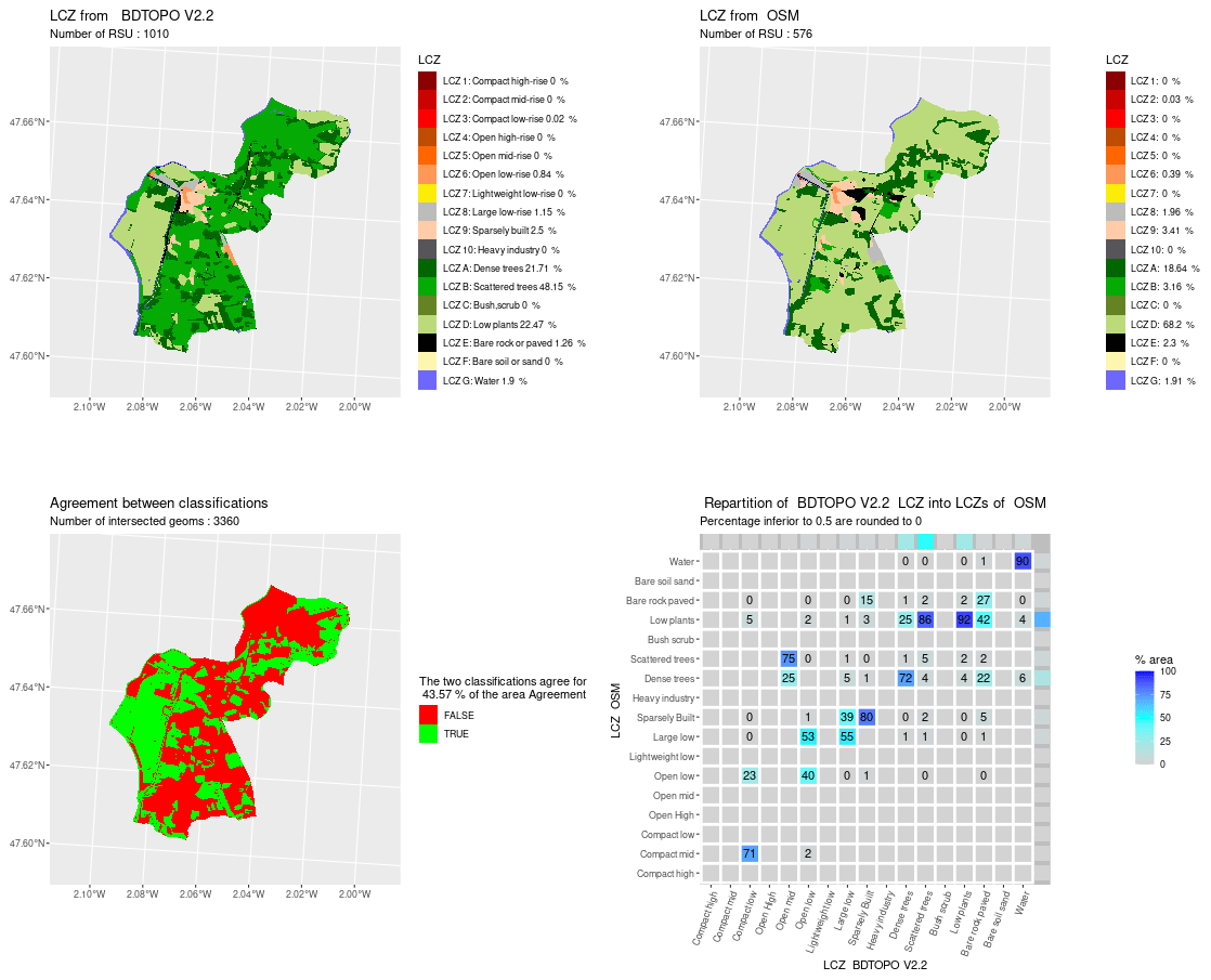
Figure 6Comparison of LCZ generated for the city of Saint-Nicolas-de-Redon by the GeoClimate method using BDT and OSM datasets.
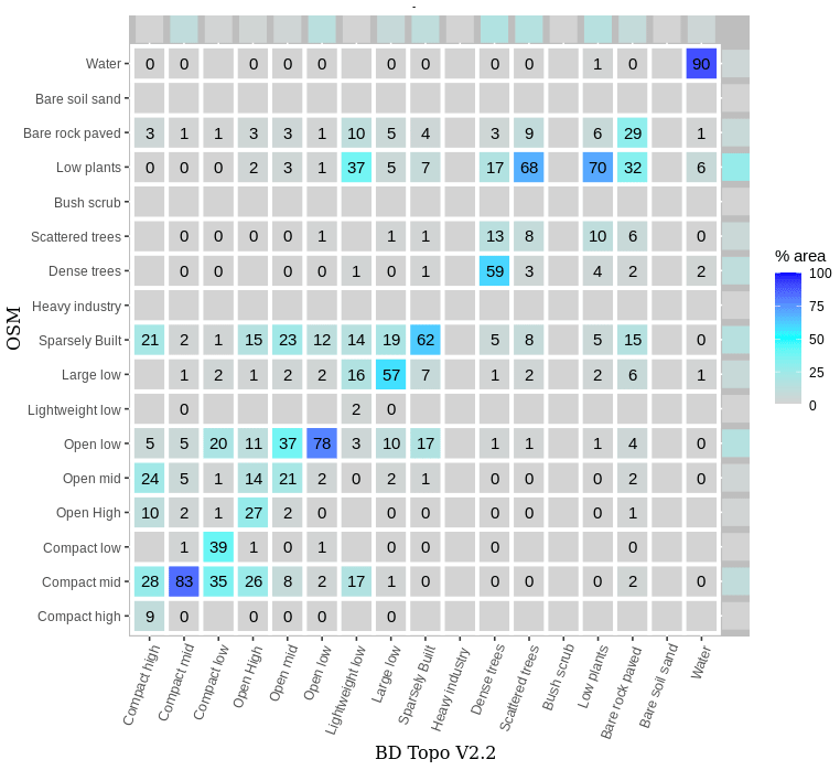
If we gather LCZ types into urban (all LCZ built types plus the bare rock and paved class) and rural classes (the rest of the LCZ land types) and compare the results obtained using OSM to the ones obtained using BDT, the degree of agreement is 87 % on average when considering all cities. If we consider the agreement between LCZ type by LCZ type, over 55 % of all territories area has the same LCZ classification between OSM and BDT. This statistic may differ a lot by territory but also by LCZ type. The best agreements are found for open low-rise and compact mid-rise (which are the more common LCZ built types), as well as water with 79 %, 81 %, and 91 %, respectively (Fig. 7). The worst agreements are found for lightweight low-rise (1 %), scattered trees (7 %), compact high-rise (8 %), open mid-rise (19 %), open high-rise (21 %), and paved (29 %), but only scattered trees and paved represent a non-negligible area (15 % and 8 % with BDT input, with none of the others above 2 % of the total area). The majority of the scattered trees in BDT RSU has been classified as low plant in OSM. This difference is clearly attributable to the spatial resolution of the datasets, since many small patches of forest are identified only in the BDT. Respectively, 68 % and 73 % of open mid-rise and open high-rise in BDT are classified as lower-rise types in OSM. This outcome is probably due to the model used to estimate OSM building height, which often produces underestimations of mid- and high-rise buildings in open areas (Bernard et al., 2022).
3.3 Uncertainty indicator
For all urban classes except large low-rise and heavy industry, an uncertainty indicator called a uniqueness value has been calculated (see Eq. 1). The higher the uniqueness value, the more certain the LCZ type attributed to a RSU. A value of 25 % seems to be a reasonable threshold to filter out uncertain values. Above this threshold (more than 40 % of the RSU), the agreement between OSM and BDT LCZ is higher than 90 %, while the agreement below the threshold is about 50 % (Fig. 8). Note that this result is only valid for RSUs with a uniqueness value. For those that do not have one, the average agreement is about 45 %.
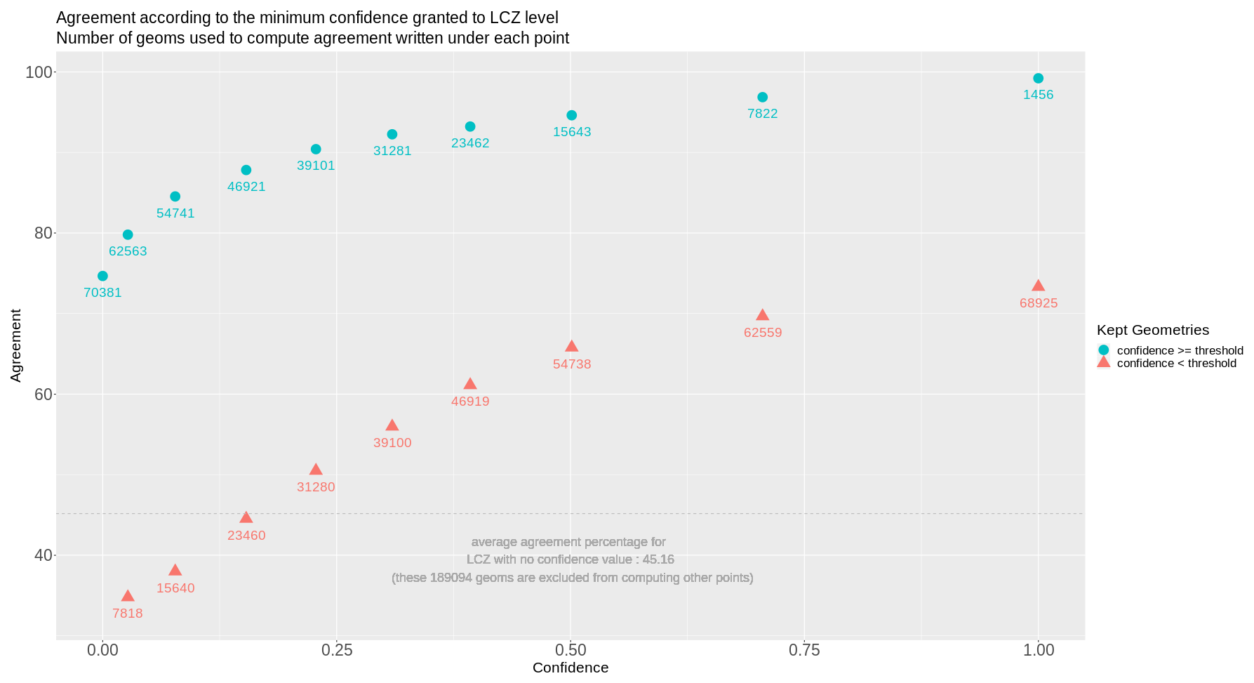
Figure 8General agreement according to the minimum confidence granted to OSM or BDT LCZ attribution.
The confidence threshold does not have the same impact for all LCZ types (Fig. 8). For those having already a quite good agreement, such as compact mid-rise, the agreement fraction cannot increase much with the confidence threshold. Setting a threshold to 0.25 increases the agreement between OSM and BDT from about 90 % to 98 %, but on the other hand, about 75 % of the RSUs that will be filtered out (50 % of the total) show agreement between BDT and OSM LCZ. On the contrary, it has a positive impact for LCZ types with a low agreement (such as open high-rise); setting a threshold to 0.25 will increase the agreement from 30 % to more than 60 %. This filter will remove more than 70 % of the RSU set as open high-rise, with only 25 % of them having agreement between BDT and OSM.
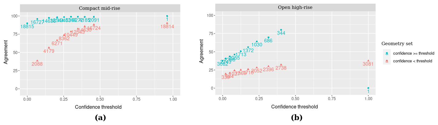
Figure 9Agreement according to the minimum confidence granted to OSM or BDT LCZ attribution (a) when LCZ is compact mid-rise and (b) when LCZ is open high-rise.
Concerning non-urbanized LCZ types, a major indicator of confidence is the fraction of non-defined land. This fraction is calculated at the RSU scale and is called the UNDEFINED_FRACTION. As expected from preliminary investigations, the OSM data have a higher land coverage; on average, for the 22 territories used as study areas, the fraction of undefined land is 37 % in OSM compared to 55 % in BDT.
3.4 City specificities
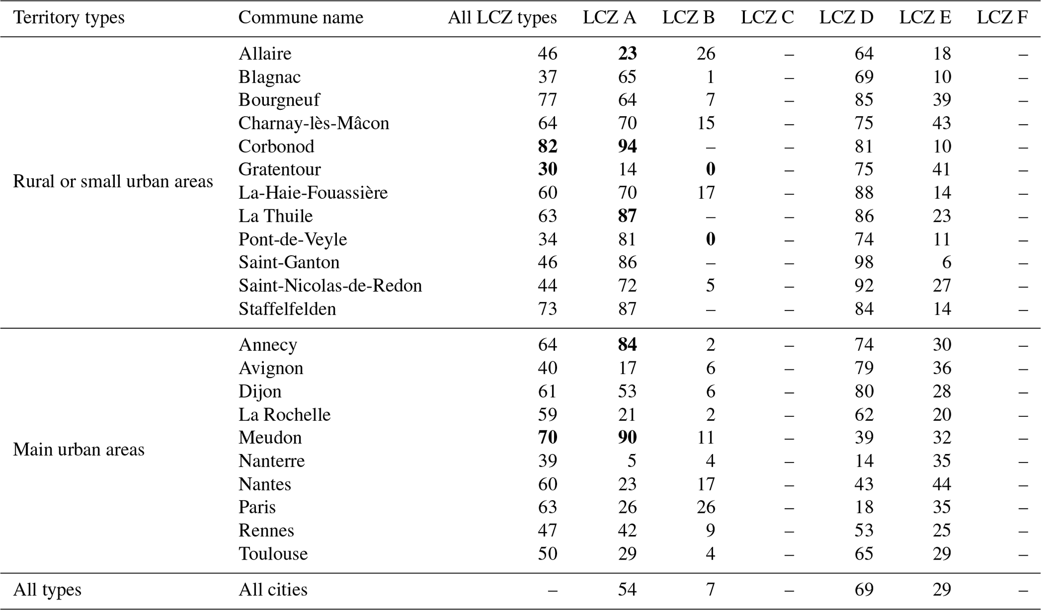
The agreement fraction by city is on average 55 % and varies from 30 % (Gratentour) to 82 % (Corbonod; see Tables 3 and 4). Most of the very low scores for rural or small urban areas are found for territories having small patches of high vegetation. As previously discussed in Sect. 3.2, only BDT demonstrates this level of detail. Territories containing small patches of vegetation (most of them being agricultural lands) are then identified as dense trees or scattered trees in BDT instead of low plants in OSM. This is the case for Allaire, which has only 23 % agreement for areas covered by dense trees in BDT, while it represents 20 % of its territory area, but also for Gratentour and Pont-de-Veyle, which both have no agreement for areas covered by scattered trees in BDT, while it represents, respectively, 53 % and 43 % of their territory area. For territories with large and homogeneous vegetation types, the general agreement is much better. This is the case for forested areas such as Corbonod (or La Thuile); 65 % (62 %) of its territory is covered by dense trees in BDT, and it has 94 % (87 %) agreement with OSM data for this specific land type.
Concerning main urban areas, the agreement between OSM and BDT is partially correlated to the fraction of their natural land and its corresponding type (Tables 3 and 4). Annecy and Meudon show the highest agreement fraction (64 % and 70 %) and have, respectively, 31 % and 45 % of their territory covered by a large and homogeneous patch of dense trees (thus having 84 % and 90 % agreement fractions). However, their agreement fraction for most of the mid- and high-rise LCZ types is very low. As described by Bernard et al. (2022), Annecy and Meudon are two cities for which the model used to estimate OSM building height fails quite a lot. This is clearly highlighted by their very low agreement for compact mid-rise LCZ (47 % for Annecy and 40 % for Meudon, while the average is 81 %). On the contrary, Paris is the city with the highest agreement for almost all mid-rise and high-rise LCZ types. The reason is twofold: many Paris building have a height tag in OSM, and most of the Paris urban fabric has quite a homogeneous structure (Haussmannian architecture , with large blocks of buildings of regular height with internal courtyards), which has been well caught by the building height model. However, if low-rise buildings are in general overestimated by the model, then it is particularly the case for Paris, where the agreement fraction for compact low-rise (LCZ3), open low-rise (LCZ6), and large low-rise (LCZ8) buildings are, respectively, 23 %, 40 %, and 40 % lower in Paris than the average for these classes.
Table 3Percentage of agreement using BDT and OSM data for urban LCZ types. Bold is used to highlight values that are interesting and that are discussed in the text.
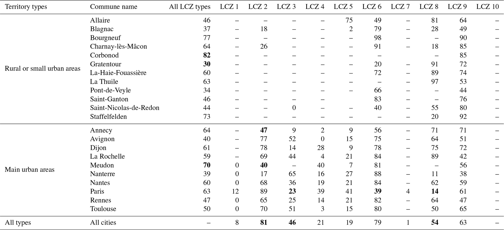
Table 4Percentage of agreement using BDT and OSM data for rural LCZ types. Bold is used to highlight values that are interesting and that are discussed in the text.
According to Quan and Bansal (2021), two main streams coexist to identify local climate zones. The first, based on images and supervised training, is applicable everywhere. However, the training is performed using expert classifications that might be quite subjective and induce a potential bias between the resulting classification and the LCZ referential, as defined by Stewart and Oke (2012). The second stream is based on UCP values calculated using geographical data, resulting in a classification in which the link with the LCZ referential is easier to make. The main shortcomings of the work presented in the literature for this second stream concern (i) datasets which are limited to a certain area (often a commune or a country) and (ii) methodologies that are often partially described and thus limited regarding their reproducibility. We presented a new method belonging to this stream that tries to address these limitations. The method described in this article can be reproduced by anyone, since it is integrated in the free and open-source software GeoClimate. It can be applied anywhere using OpenStreetMap data, which are available worldwide.
GeoClimate is designed to work with any dataset. Currently, it can automatically calculate LCZ using OSM and BDT data (a French national dataset). After a detailed description of the algorithm implemented in GeoClimate, it is applied to 22 French communes to compare the LCZ produced using OSM and BDT data. About 55 % of the area of all studied territories has obtained the same LCZ type. The agreement fraction between OSM and BDT classification varies greatly between the communes (from 30 % to 82 %). Large patches of forest and water are well indexed in both data sources, thus leading to a good agreement for territories containing a large share of these land types. Concerning LCZ built types, the agreement is high for compact mid-rise and open low-rise (83 % and 78 %, respectively) which are the main LCZ built types. However, a large part of the RSU classified into open mid-rise and open high-rise using BDT are set to open low-rise using OSM. This difference is attributed to the height underestimation for OSM buildings located in open areas (see Bernard et al., 2022).
Whenever a LCZ built type (except LCZ8 and LCZ10) is attributed to a RSU, a confidence indicator called LCZ_UNIQUENESS_VALUE is calculated. The agreement between OSM and BDT increases substantially when we only consider that RSU has a larger confidence value. Using a confidence threshold of 0.25 when mapping LCZ with the GeoClimate method is a good way to ensure that the LCZ type attributed to a RSU is reasonably accurate, while minimizing the number of RSUs removed from the analysis. This threshold only applied to some LCZ built types. There is currently no confidence indicator for LCZ8 or LCZ10, which might be a source of improvement for future versions of this work. Concerning non-urbanized LCZ types, a good indicator of confidence is the fraction of undefined land. This information is produced by GeoClimate for each RSU under the name UNDEFINED_FRACTION. Above 50 % of the UNDEFINED_FRACTION, we may assume that the attribution of a given LCZ is quite random. Moreover, some land types are currently not defined in GeoClimate (bare soil, sand, bush, and scrubs), which causes missing LCZ types (C and F). These should soon be integrated in a future GeoClimate version. Quan and Bansal (2021) have identified six steps that are classically used in vector-based approaches for LCZ classification. The four first steps used in the GeoClimate methodology have been presented, and the limitations corresponding to each dataset used as input identified. Potential future work could be to propose a methodology to aggregate small RSU into bigger ones to reach the minimal LCZ unit size of 400 m wide (step 5) and then compare the resulting LCZ to climate data provided by observations or models (step 6).
The GeoClimate software has great potential for new collaborations. Along with the lczexplore R package, it can be used to efficiently compare the LCZ produced with GeoClimate to any other method. The influence of each step of the LCZ creation can be investigated separately, including the impact of the dataset (as presented in this paper), of the unit of analysis (RSU), of the method used for UCPs calculation, and of the algorithm used to assign a LCZ. GeoClimate also has the potential to interact with the current WUDAPT approach. While GeoClimate may be used to train the WUDAPT model on areas in which the results are quite confident, WUDAPT can in turn be used on areas for which OSM data are still quite poor. To confirm the complementarity between these two workflows, a more in-depth study of their differences on similar locations needs to be performed.
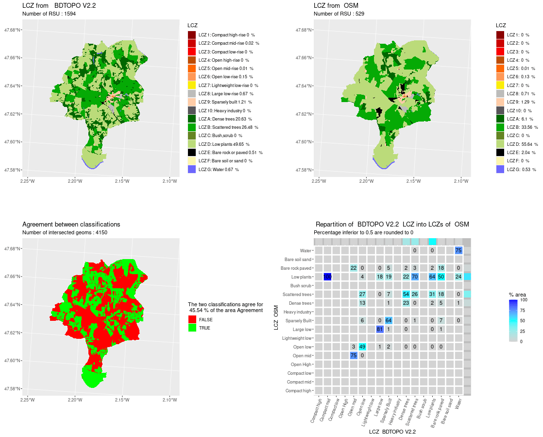
Figure A1Comparison of LCZ generated for the city of Allaire by the GeoClimate method using BDT and OSM datasets.
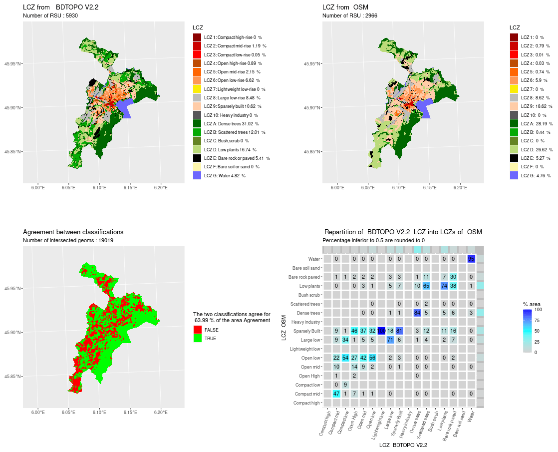
Figure A2Comparison of LCZ generated for the city of Annecy by the GeoClimate method using BDT and OSM datasets.
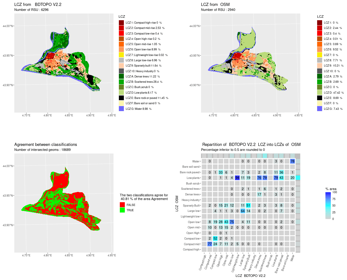
Figure A3Comparison of LCZ generated for the city of Avignon by the GeoClimate method using BDT and OSM datasets.
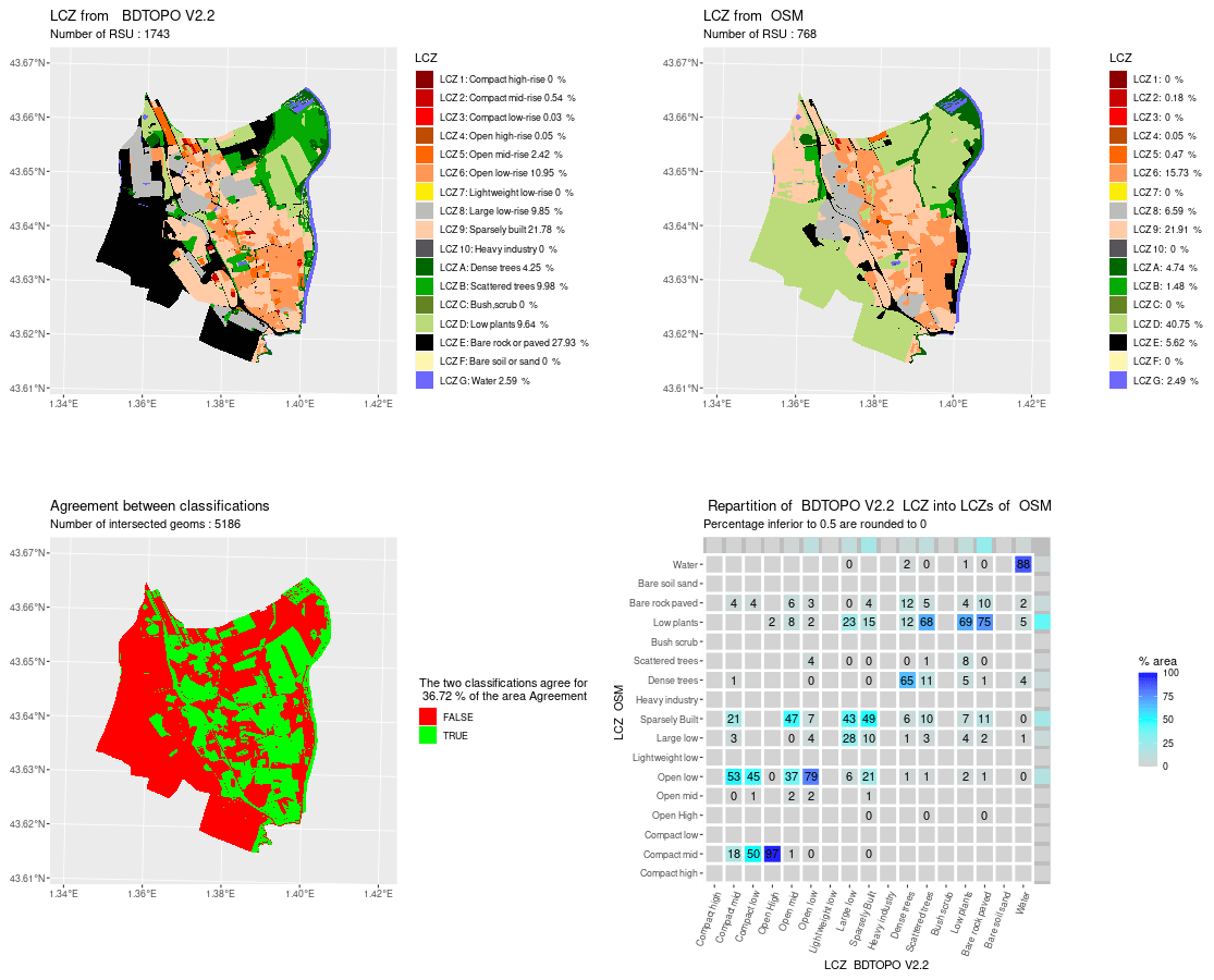
Figure A4Comparison of LCZ generated for the city of Blagnac by the GeoClimate method using BDT and OSM datasets.
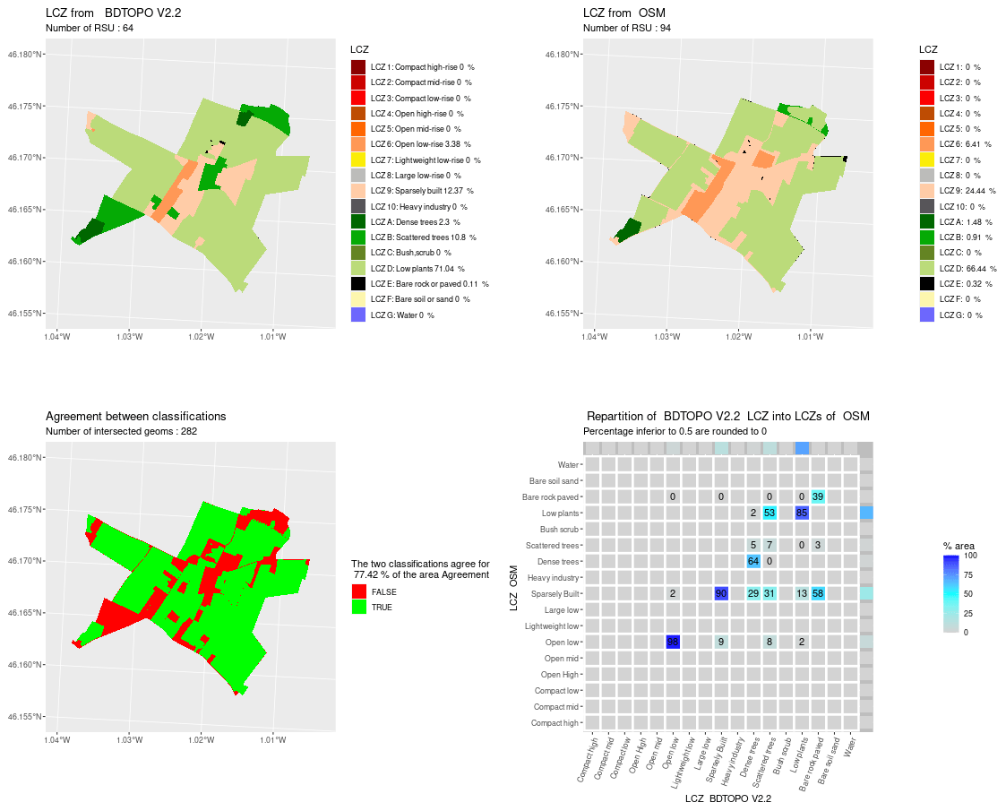
Figure A5Comparison of LCZ generated for the city of Bourgneuf by the GeoClimate method using BDT and OSM datasets.
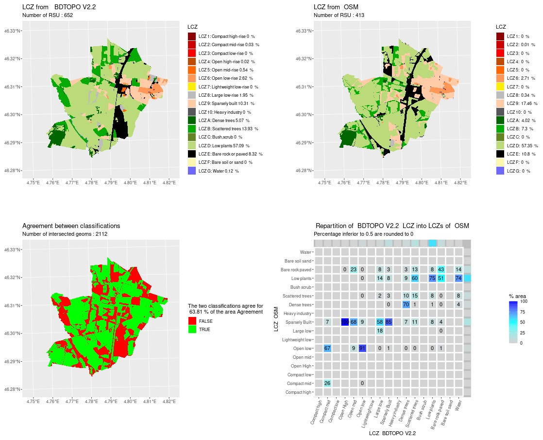
Figure A6Comparison of LCZ generated for the city of Charnay-lès-Mâcon by the GeoClimate method using BDT and OSM datasets.
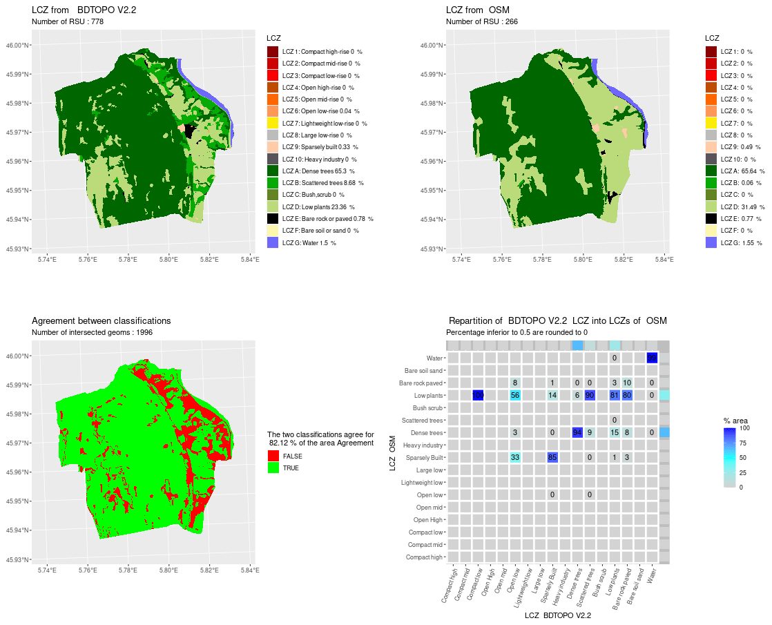
Figure A7Comparison of LCZ generated for the city of Corbonod by the GeoClimate method using BDT and OSM datasets.

Figure A8Comparison of LCZ generated for the city of Dijon by the GeoClimate method using BDT and OSM datasets.
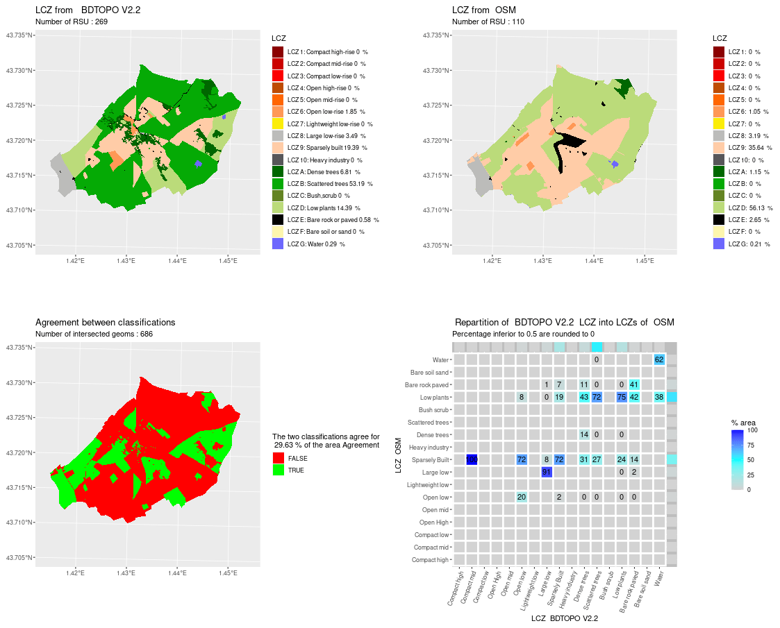
Figure A9Comparison of LCZ generated for the city of Gratentour by the GeoClimate method using BDT and OSM datasets.
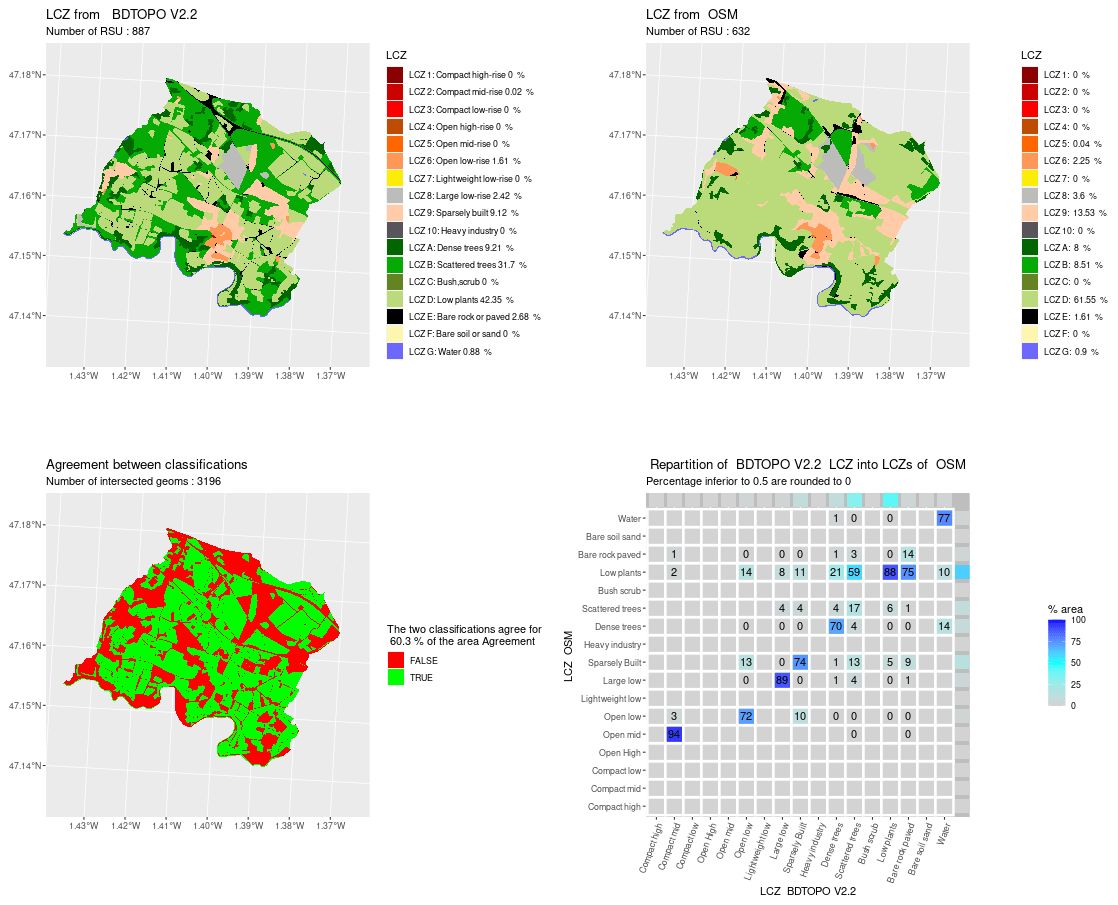
Figure A10Comparison of LCZ generated for the city of La Haie-Fouassière by the GeoClimate method using BDT and OSM datasets.
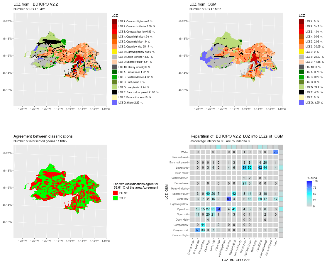
Figure A11Comparison of LCZ generated for the city of La Rochelle by the GeoClimate method using BDT and OSM datasets.
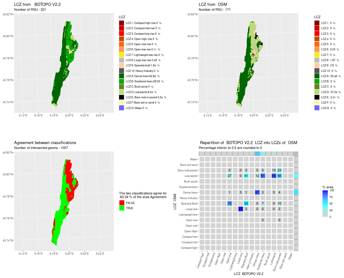
Figure A12Comparison of LCZ generated for the city of La Thuile by the GeoClimate method using BDT and OSM datasets.
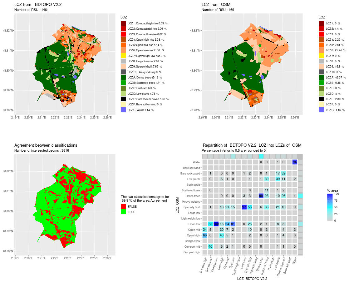
Figure A13Comparison of LCZ generated for the city of Meudon by the GeoClimate method using BDT and OSM datasets.
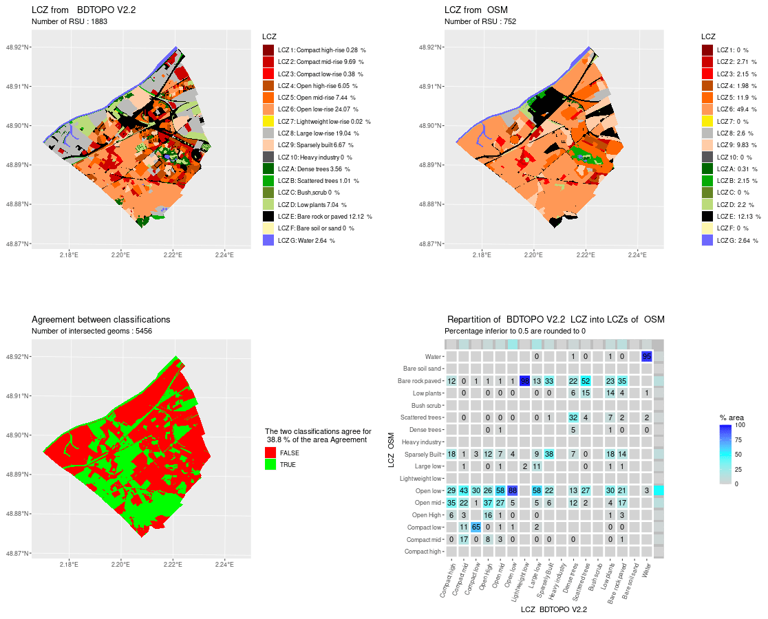
Figure A14Comparison of LCZ generated for the city of Nanterre by the GeoClimate method using BDT and OSM datasets.
Figure A15Comparison of LCZ generated for the city of Nantes by the GeoClimate method using BDT and OSM datasets.
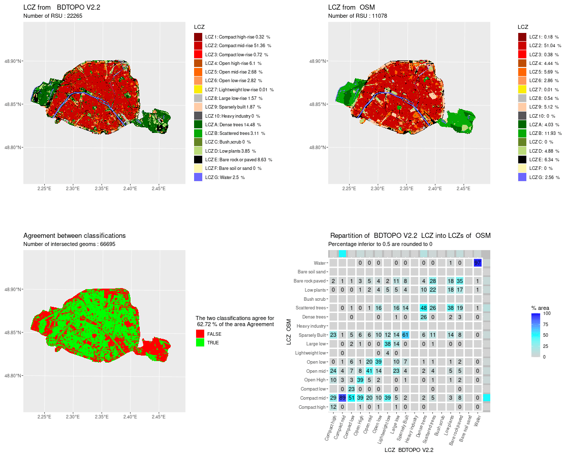
Figure A16Comparison of LCZ generated for the city of Paris by the GeoClimate method using BDT and OSM datasets.
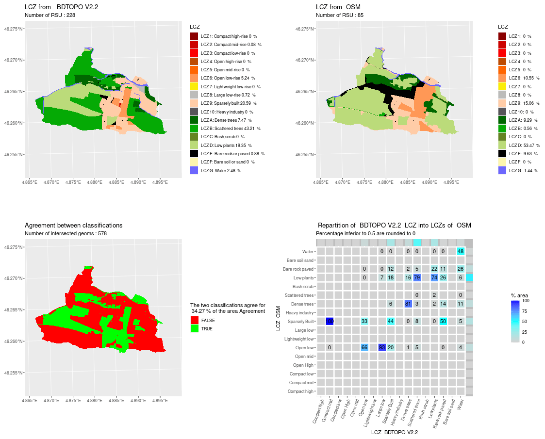
Figure A17Comparison of LCZ generated for the city of Pont-de-Veyle by the GeoClimate method using BDT and OSM datasets.
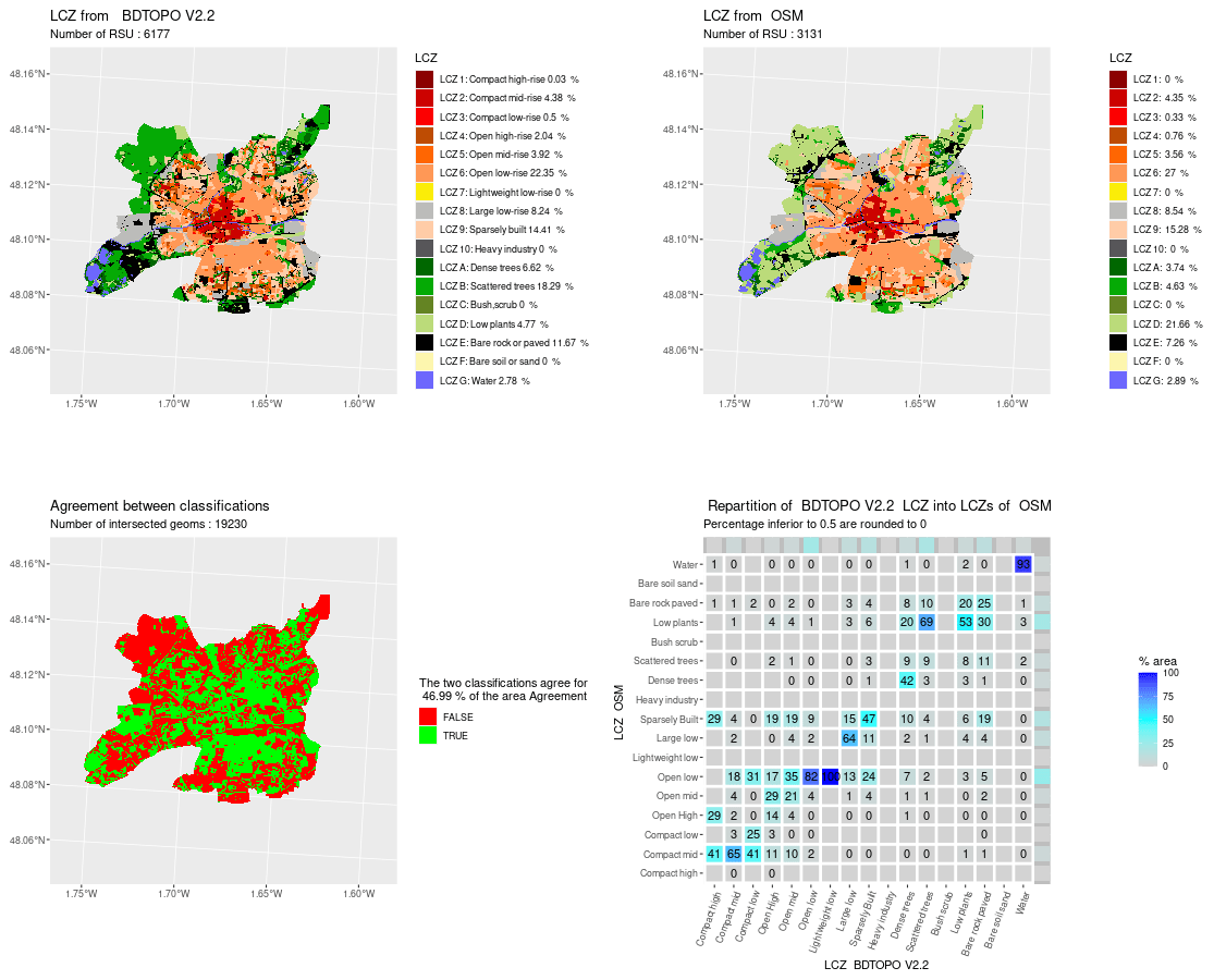
Figure A18Comparison of LCZ generated for the city of Rennes by the GeoClimate method using BDT and OSM datasets.
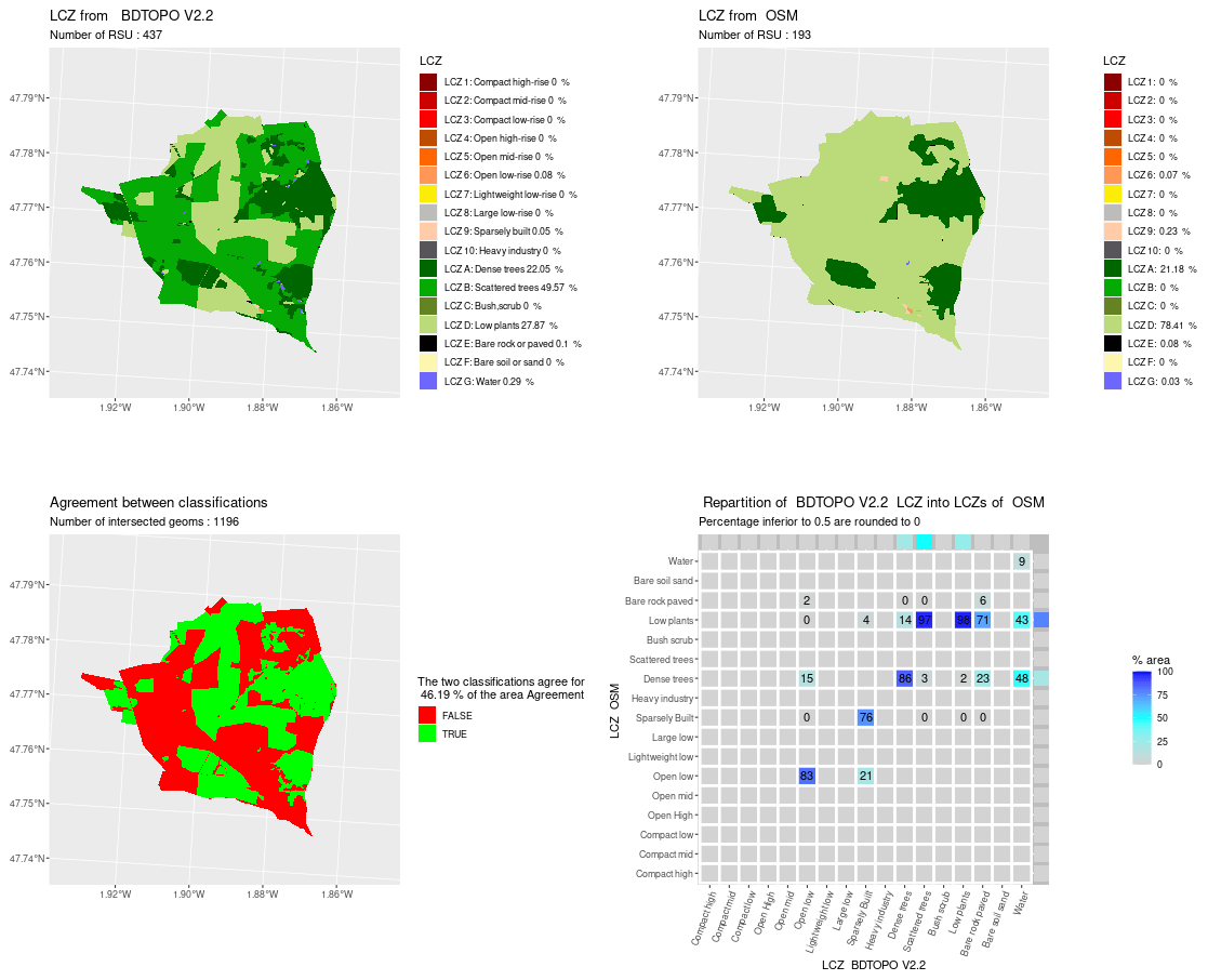
Figure A19Comparison of LCZ generated for the city of Saint-Ganton by the GeoClimate method using BDT and OSM datasets.
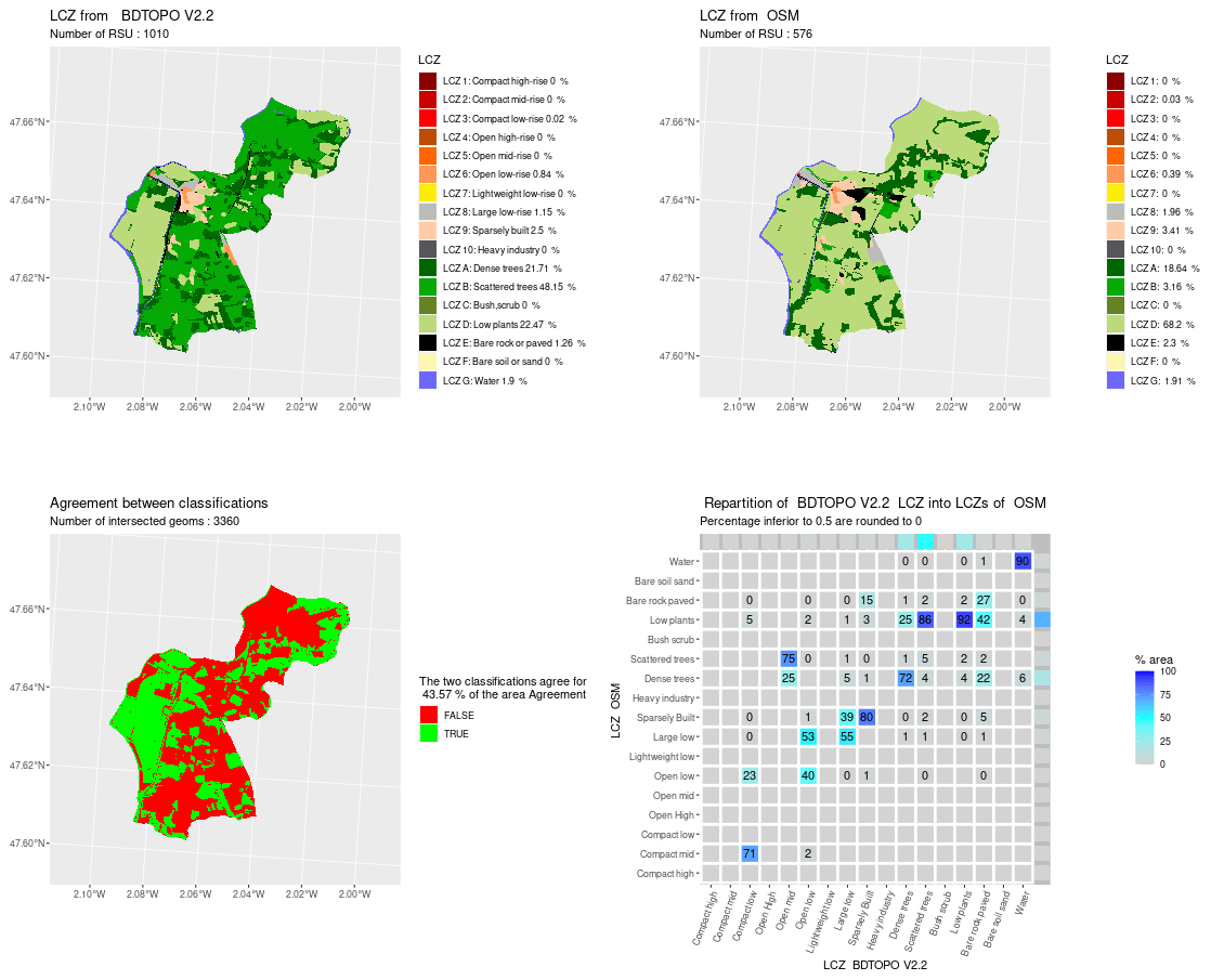
Figure A20Comparison of LCZ generated for the city of Saint-Nicolas-de-Redon by the GeoClimate method using BDT and OSM datasets.
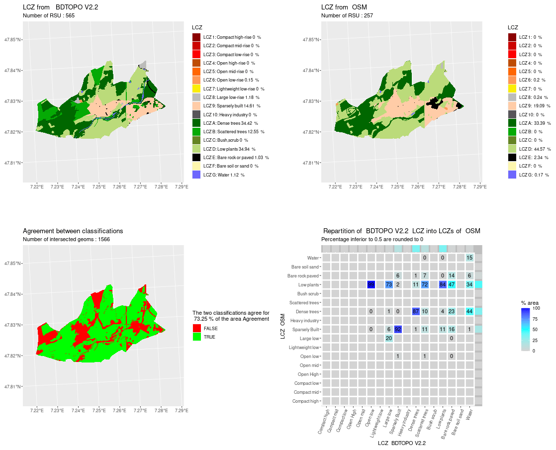
Figure A21Comparison of LCZ generated for the city of Staffelfelden by the GeoClimate method using BDT and OSM datasets.
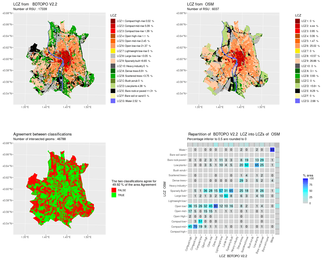
Figure A22Comparison of LCZ generated for the city of Toulouse by the GeoClimate method using BDT and OSM datasets.
The LCZ calculation is performed using the GeoClimate 0.0.1 software available at https://doi.org/10.5281/zenodo.6372337 (Bocher et al., 2022), while the figures used in the paper were created using the lczexplore R package available at https://doi.org/10.5281/zenodo.7646866 (Gousseff, 2023). All the work performed in this paper can be reproduced by following the Readme file of the following Zenodo repository: https://doi.org/10.5281/zenodo.7687911 (Bernard et al., 2023).
Conceptualization: JB, EB, and FL. Data curation: JB, EB, MG, and FL. Formal analysis: MG, JB, EB, and FL. Funding acquisition: EB and JB. Investigation: JB, EB, MG, and FL. Methodology: JB and EB. Project administration: JB and EB. Resources: EB. Software: EB, JB, MG, FL, and ELSW. Supervision: JB and EB. Validation: EB, JB, MG, FL, and ELSW. Visualization: MG, JB, EB, and FL. Original draft preparation: JB, FL, and EB. Review and editing: FL, MG, JB, and EB.
The contact author has declared that none of the authors has any competing interests.
Publisher's note: Copernicus Publications remains neutral with regard to jurisdictional claims made in the text, published maps, institutional affiliations, or any other geographical representation in this paper. While Copernicus Publications makes every effort to include appropriate place names, the final responsibility lies with the authors.
This research has been supported by the European Commission, Horizon 2020 (grant no. 896069), and the Agence de l'Environnement et de la Maîtrise de l'Energie (PAENDORA2; PACT2e 2021 research call).
The article processing charges for this open-access publication were covered by the Gothenburg University Library.
This paper was edited by Le Yu and reviewed by Jan Geletic and three anonymous referees.
Baklanov, A., Cárdenas, B., Lee, T.-C., Leroyer, S., Masson, V., Molina, L. T., Müller, T., Ren, C., Vogel, F. R., and Voogt, J. A.: Integrated urban services: Experience from four cities on different continents, Urban Clim., 32, 100610, https://doi.org/10.1016/j.uclim.2020.100610, 2020. a
Bernard, J., Bocher, E., Petit, G., and Palominos, S.: Sky view factor calculation in urban context: computational performance and accuracy analysis of two open and free GIS tools, Climate, 6, 60, https://doi.org/10.3390/cli6030060, 2018. a
Bernard, J., Bocher, E., Le Saux Wiederhold, E., Leconte, F., and Masson, V.: Estimation of missing building height in OpenStreetMap data: a French case study using GeoClimate 0.0.1, Geosci. Model Dev., 15, 7505–7532, https://doi.org/10.5194/gmd-15-7505-2022, 2022. a, b, c, d, e
Bernard, J., Bocher, E., Gousseff, M., Wiederhold, L. S., and Leconte, F.: GeoClimate 0.0.1 LCZ calculation: Code and data, Zenodo [code and data set], https://doi.org/10.5281/zenodo.7687911, 2023. a, b
Bocher, B., Wiederhold, L. S., Leconte, Petit, Palominos, and Noûs: GeoClimate: a Geospatial processing toolbox for environmental and climate studies, Zenodo [code], https://doi.org/10.5281/zenodo.6372337, 2022. a, b
Bocher, E., Bernard, J., Wiederhold, E. L. S., Leconte, F., Petit, G., Palominos, S., and Noûs, C.: GeoClimate: a Geospatial processing toolbox for environmental and climate studies, J. Open Source Softw., 6, 3541, https://doi.org/10.21105/joss.03541, 2021. a, b, c, d, e
Ching, J., Mills, G., Bechtel, B., See, L., Feddema, J., Wang, X., Ren, C., Brousse, O., Martilli, A., Neophytou, M., Mouzourides, P., Stewart, I., Hanna, A., Ng, E., Foley, M., Alexander, P., Aliaga, D., Niyogi, D., Shreevastava, A., Bhalachandran, P., Masson, V., Hidalgo, J., Fung, J., Andrade, M., Baklanov, A., Dai, W., Milcinski, G., Demuzere, M., Brunsell, N., Pesaresi, M., Miao, S., Mu, Q., Chen, F., and Theeuwes, N.: WUDAPT: An urban weather, climate, and environmental modeling infrastructure for the anthropocene, B. Am. Meteorol. Soc., 99, 1907–1924, 2018. a
Davenport, A. G., Grimmond, C. S. B., Oke, T. R., and Wieringa, J.: Estimating the roughness of cities and sheltered country, in: Preprints, 12th Conf. on Applied Climatology, Asheville, NC, Amer. Meteor. Soc, vol. 96, p. 99, https://ams.confex.com/ams/May2000/webprogram/Paper13744.html (last access: 4 March 2024), 2000. a
Demuzere, M., Bechtel, B., Middel, A., and Mills, G.: Mapping Europe into local climate zones, PloS one, 14, e0214474, https://doi.org/10.1371/journal.pone.0214474, 2019. a
Demuzere, M., Hankey, S., Mills, G., Zhang, W., Lu, T., and Bechtel, B.: Combining expert and crowd-sourced training data to map urban form and functions for the continental US, Sci. Data, 7, 264, https://doi.org/10.1038/s41597-020-00605-z, 2020. a
Demuzere, M., Kittner, J., and Bechtel, B.: LCZ Generator: a web application to create Local Climate Zone maps, Front. Environ. Sci., 9, 637455, https://doi.org/10.3389/fenvs.2021.637455, 2021. a
Geletič, J., Lehnert, M., and Dobrovolnỳ, P.: Land surface temperature differences within local climate zones, based on two central European cities, Remote Sens., 8, 788, https://doi.org/10.3390/rs8100788, 2016. a
Gousseff, M. lczexplore: an R package to compare different local climate zone classifications on same geographical areas, Zenodo [code], https://doi.org/10.5281/zenodo.7646866, 2023. a, b
Grimmond, S., Bouchet, V., Molina, L. T., Baklanov, A., Tan, J., Schlünzen, K. H., Mills, G., Golding, B., Masson, V., Ren, C., Voogt, J., Miao, S., Lean, H., Heusinkveld, B., Hovespyan, A., Teruggi, G., Parrish, P., and Joe, P.: Integrated urban hydrometeorological, climate and environmental services: Concept, methodology and key messages, Urban Clim., 33, 100623, https://doi.org/10.1016/j.uclim.2020.100623, 2020. a
Hanna, S. R. and Britter, R. E.: Wind flow and vapor cloud dispersion at industrial and urban sites, John Wiley & Sons, ISBN 0-8169-0863-X, 2010. a
IPCC: The physical science basis. Contribution of working group I to the fourth assessment report of the Intergovernmental Panel on Climate Change, Cambridge University Press, Cambridge, United Kingdom and New York, NY, USA, 996, 113–119, ISBN 9781107661820, 2007. a, b
Leconte, F., Bouyer, J., Claverie, R., and Pétrissans, M.: Using Local Climate Zone scheme for UHI assessment: Evaluation of the method using mobile measurements, Build. Environ., 83, 39–49, https://doi.org/10.1016/j.buildenv.2014.05.005, 2015. a
Masson, V., Heldens, W., Bocher, E., Bonhomme, M., Bucher, B., Burmeister, C., de Munck, C., Esch, T., Hidalgo, J., Kanani-Sühring, F., Kwok, J.-T., Lemonsu, A., Lévy, J.-P., Maronga, B., Pavlik, D., Petit, G., See, L., Schoetter, R., Tornay, N., Votsis, A., and Zeidler, J.: City-descriptive input data for urban climate models: Model requirements, data sources and challenges, Urban Clim., 31, 100536, https://doi.org/10.1016/j.uclim.2019.100536, 2020. a
Quan, S. J. and Bansal, P.: A systematic review of GIS-based local climate zone mapping studies, Build. Environ., 196, 107791, https://doi.org/10.1016/j.buildenv.2021.107791, 2021. a, b, c, d, e, f
Quan, S. J., Dutt, F., Woodworth, E., Yamagata, Y., and Yang, P. P.-J.: Local climate zone mapping for energy resilience: a fine-grained and 3D approach, Enrgy. Proced., 105, 3777–3783, 2017. a
Skarbit, N., Stewart, I. D., Unger, J., and Gál, T.: Employing an urban meteorological network to monitor air temperature conditions in the “local climate zones” of Szeged, Hungary, Int. J. Climatol., 37, 582–596, 2017. a
Stewart, I. D.: Redefining the urban heat island, Ph. D. thesis, University of British Columbia, https://doi.org/10.14288/1.0072360, 2011. a
Stewart, I. D. and Oke, T. R.: Local climate zones for urban temperature studies, B. Am. Meteorol. Soc., 93, 1879–1900, 2012. a, b, c, d, e, f, g, h, i, j