the Creative Commons Attribution 4.0 License.
the Creative Commons Attribution 4.0 License.
 | 05 Mar 2024
Three-dimensional geological modelling of igneous intrusions in LoopStructural v1.5.10
Fernanda Alvarado-Neves
Laurent Ailleres
Lachlan Grose
Alexander R. Cruden
Robin Armit
Over the last 2 decades, there have been significant advances in the 3D modelling of geological structures via the incorporation of geological knowledge into the model algorithms. These methods take advantage of different structural data types and do not require manual processing, making them robust and objective. Igneous intrusions have received little attention in 3D modelling workflows, and there is no current method that ensures the reproduction of intrusion shapes comparable to those mapped in the field or in geophysical imagery. Intrusions are usually partly or totally covered, making the generation of realistic 3D models challenging without the modeller's intervention. In this contribution, we present a method to model igneous intrusions in 3D considering geometric constraints consistent with emplacement mechanisms. Contact data and inflation and propagation direction are used to constrain the geometry of the intrusion. Conceptual models of the intrusion contact are fitted to the data, providing a characterisation of the intrusion thickness and width. The method is tested using synthetic and real-world case studies, and the results indicate that the method can reproduce expected geometries without manual processing and with restricted datasets. A comparison with radial basis function (RBF) interpolation shows that our method can better reproduce complex geometries, such as saucer-shaped sill complexes.
- Article
(8997 KB) - Full-text XML
- BibTeX
- EndNote


Significant advances in 3D geological modelling have shown that incorporating prior geological knowledge into interpolation algorithms can significantly improve the 3D representation of the geometry of structures (e.g. Godefroy et al., 2017; Grose et al., 2018, 2019; Hillier et al., 2014; Laurent et al., 2013, 2016; Thibert et al., 2005). Geological knowledge of a geological feature can be incorporated into the 3D modelling workflow using different approaches. For instance, by parameterising its 3D geometry, defining its expected geometries, or using complete structural datasets. These approaches have been applied to folds and faults, showing substantial improvements in 3D geological models, especially in models built using few or poor-quality observations.
To the best of our knowledge, there has been no attempt to improve the 3D modelling of intrusions, and no methods exist that incorporate prior knowledge into the modelling algorithm. Implicit 3D models of intrusions are currently characterised by a surface representing its contact boundary, and this boundary is numerically described using the same frameworks as those used to build other geological interfaces, such as stratigraphic contacts or faults (Wellmann and Caumon, 2018; Calcagno et al., 2008). However, intrusions' geometry differs from these geological features because they are closed surfaces that are not continuous in the 3D space. Two types of constraints are generally applied to build 3D models of igneous intrusions: (1) point data that indicate the location of the contact between the intrusion and the host rock and (2) a polarity constraint, which is a vector indicating the direction from the outside to the inside of the intrusion (Calcagno et al., 2008). The distinction between the top and base contact of the intrusion and other field measurements, such as the inflation and flow direction of the magma, are not considered to constrain the models. While the polarity constraint helps to adapt current interpolation methods to intrusions, it is not measurable in the field and does not have any geological meaning.
Igneous intrusions, such as plutons, laccoliths, sills, and layered intrusions, develop tabular bodies, with their horizontal dimension greater than their vertical dimension (e.g. Cruden et al., 2017, 1999; McCaffrey and Petford, 1997; Vigneresse et al., 1999). Their geometries and locations in the crust are strongly controlled by the anisotropies of the host rock that facilitated their emplacement, such as bedding and faults (e.g. Barnett and Gudmundsson, 2014; Brun and Pons, 1981; Clemens and Mawer, 1992; Gudmundsson, 2011; Morgan, 2018; Souche et al., 2019). While intrusions' 3D models estimated with existing methods are consistent with contact observations, they may not honour the tabular nature of intrusions without manual processing in data-sparse environments. In particular, the intrusion shape and its geometrical relation with the host rock are unlikely to be captured away from the data. This is particularly important for 3D models of intrusions, as they are usually only partly exposed, if not totally covered, and are consequently inferred from geophysical interpretations or simulations; moreover, intrusion observations (location and orientation of the contacts) are usually sparse.
To improve the 3D representation of intrusions, we propose a general workflow inspired by the object-distance simulation method (ODSIM; Henrion et al., 2008, 2010). Our method integrates conceptual knowledge of magma emplacement mechanisms into the ODSIM framework, enabling the reproduction of intrusion geometries comparable to those observed in reality. As these concepts are integrated into the methodological framework, the results are objective and reproducible. In practice, the method can use different types of datasets, build models of different types of intrusions, and incorporate knowledge of magma's mechanical behaviour into a purely geometric approach. The approach has three main steps. We initially build a structural frame adapted for intrusions (Grose et al., 2021a, b). This object is a curvilinear coordinate system whose main axis represents the location of the intrusion's top (or base) contact. The intrusion frame is constrained using contact data, the geometry of the host rock's foliation and/or structures that facilitated the emplacement of the intrusion, and vector directions indicating the propagation and growth of the magma. Then, conceptual models describing the coarse-scale geometry of the intrusion are parameterised using the intrusion frame coordinates and are employed to characterise the contact geometry along its axes. Finally, we use the conceptual models to modify the intrusion frame scalar fields to obtain a unique scalar field whose isovalue zero represents the intrusions' contact boundary.
This contribution is organised as follows. First, we summarise intrusion emplacement mechanisms and geometries of intrusions, with a specific focus on those features that can be used as geometric parameters for 3D modelling. Secondly, we introduce the method developed in this work and its association with previous work. Thirdly, we show the results of the application of the method in three case studies: a laccolith, a pluton, and a sill complex. Then, we assess the value of this method by comparing the resulting 3D model of a sill intrusion with its 3D model built using a classical interpolation framework. Finally, we discuss the advantages of adding geological knowledge of intrusions in the modelling framework, the limitations of our method, and further work that can be done to improve this approach.
Igneous intrusions comprise a significant volume of the Earth's crust and are found in all tectonic settings. They are part of volcanic and igneous plumbing systems, which involve magma production, transport, and emplacement (Burchardt, 2018). Magma production occurs due to partial melting of rocks in the upper mantle or crust (e.g. Brown, 2007; Petford et al., 2000; van Wyk de Vries and van Wyk de Vries, 2018). Magma can be vertically and laterally transported to its final emplacement location by the intrusion of dykes, sills, and inclined sheets (e.g. Brown, 2007; Magee et al., 2016). The emplacement of magma is controlled by mechanical interactions and the density contrast between the magma and its surroundings (e.g. Brown 2007; Hutton, 1988; Petford et al., 2000).
While there is a wide range of emplacement mechanisms (e.g. Paterson et al., 1996; Hutton, 1988; Miller and Paterson, 2001; Pignotta and Paterson, 2007; Galland et al., 2018; Johnson and Pollard, 1973), the geometry and location in the crust of many intrusions are strongly controlled by the anisotropies of the host rock that facilitated their emplacement, such as bedding, faults, stress barriers, and shear zones (e.g. Barnett and Gudmundsson, 2014; Brun and Pons, 1981; Hogan and Gilbert, 1995; Clemens and Mawer, 1992; Guineberteau et al., 1987; Weinberg et al., 2004). After the magma is emplaced or while it propagates through the crust, the intrusion grows.
The growth of plutons depends on host rock mechanical properties (Cruden and Weinberg, 2018) and can occur by both vertical and/or lateral displacement of the host rock (e.g. Cruden, 1998; Cruden et al., 1999; Grocott et al., 1999). Sills grow by horizontal propagation of their lateral tips and by vertical inflation (e.g. Hutton, 2009). The sill inflation direction is parallel to the intrusion opening vector, which may or may not be orthogonal to the intrusion plane (Magee et al., 2019). Laccoliths are generally developed by the incremental growth of an initial sill (e.g. Annen et al., 2015; Chen and Nabelek, 2017; Johnson and Pollard, 1973; Michel et al., 2008). The sills' top and bottom contacts act as discontinuities controlling the emplacement of new sheets (Morgan, 2018).
The geometries of intrusions have been characterised using different datasets, such as field observations of the intrusion's top, base, and lateral contacts; drilling data; and interpretation of gravity and seismic surveys (e.g. Braga et al., 2019; Cervantes, 2019; Eshaghi et al., 2016; Rawling et al., 2011; Grocott et al., 2009; Leaman, 1976, 2002; Paterson et al., 1996). There is a general agreement that intrusions develop tabular geometries in the coarse scale, with their horizontal dimensions being greater than their vertical dimension (e.g. Cruden et al., 2017, 1999; McCaffrey and Petford, 1997; Vigneresse et al., 1999). On the smaller scale, intrusions show a variety of shapes (Fig. 1). Plutons can be symmetric or asymmetric with one or more vertical feeder zones (Clemens and Mawer, 1992; Vigneresse, 1995; Vigneresse et al., 1999). In a plan view, plutons show elliptical or irregular geometry (Cruden, 1998). Their roof is roughly planar with an abrupt roof–sides transition (Paterson et al., 1996), and the floor may be wedge-shaped, dipping towards the feeder, or tablet-shaped, concordant with the roof (Cruden and McCaffrey, 2001; Cruden, 2006; Vigneresse, 1995; Vigneresse et al., 1999). Sills are sheet-like intrusions that can develop strata-concordant tabular bodies with little or no change in thickness or straight or step-wise transgressive bodies that develop an oblique angle with the host rock foliation (Galland et al., 2018; Jackson et al., 2013). Sills may also develop saucer or V shapes, with a thicker concordant inner sill that transitions to thinner transgressive outer sills (Galland et al., 2018; Köpping et al., 2022). Sill complexes are composed of elements (e.g. Köpping et al., 2022), which are generally elongated and narrow in map view, with tablet-shape or elliptical cross-sections (Leaman, 1995; Schofield et al., 2010, 2012). If two or more sill segments propagate in the same direction but at different stratigraphic levels, they eventually coalesce, developing connectors such as steps or bridges (e.g. Hutton, 2009; Köpping et al., 2022; Magee et al., 2019; Schofield et al., 2012). The laccolith roof and sides may be symmetric, developing a bell-jar shape with a slightly arched and concordant roof and outward-dipping sides (e.g. Clemens and Mawer, 1992; Johnson and Pollard, 1973; Morgan, 2018), or asymmetric with a flat roof concordant with the host rock layering and bounded by a fault on one side (e.g. de Saint-Blanquat et al., 2006). The floor of laccoliths is usually concordant with the stratigraphy with one feeder zone.
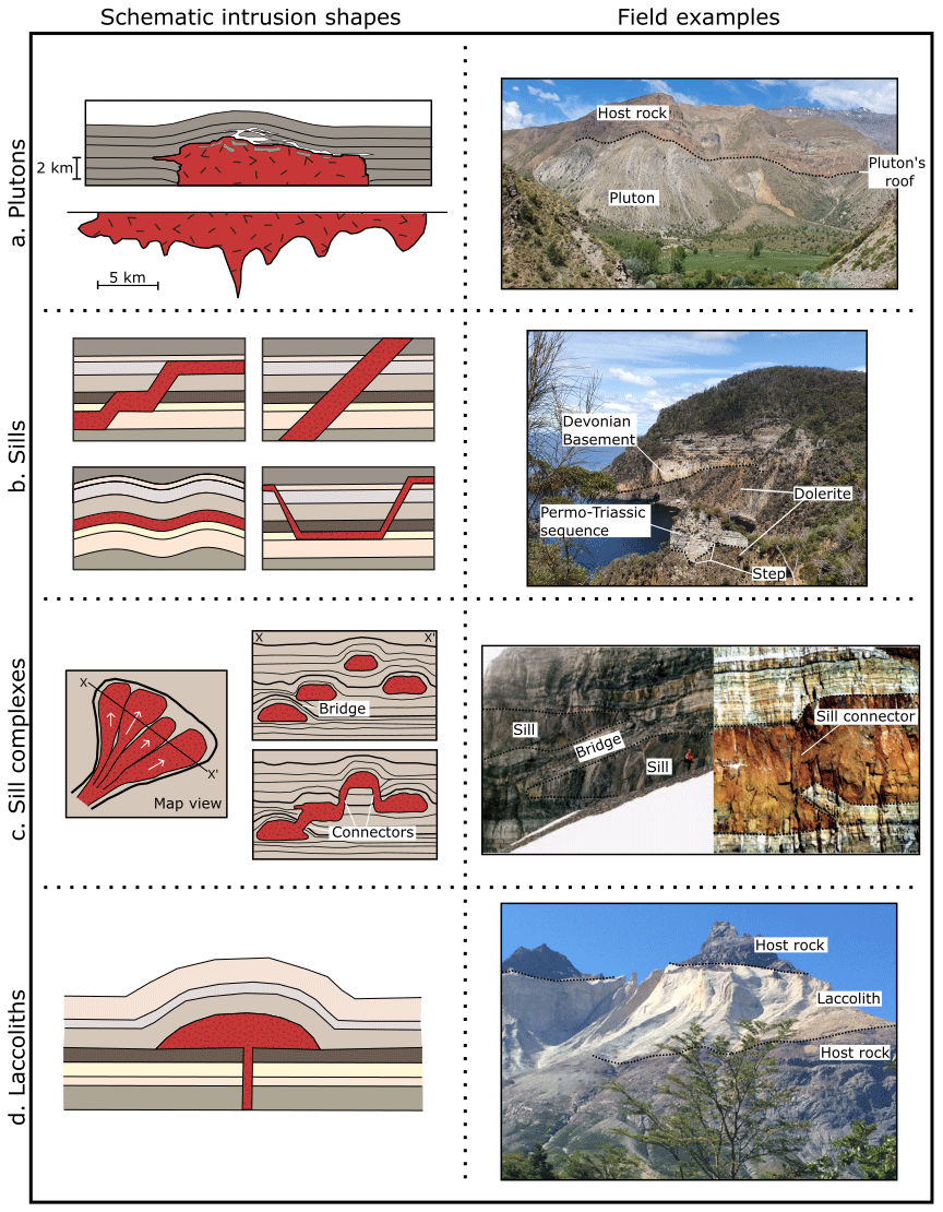
Figure 1Schematic intrusion shapes and field examples. (a) Schematic cross-section of a pluton's roof (after Paterson et al., 1996) and tablet-shaped floor contact inferred from the 3D inversion of gravity data (after Vigneresse et al., 1999). Field example showing the roof of the San Gabriel pluton emplaced in the volcano-sedimentary Abanico Formation, Maipo Valley, Central Chile. (b) Schematic morphologies of sill sheets (after Galland et al., 2018) and a field example from the roof contact of the Tasmanian dolerite emplaced in the sedimentary Parmeener Supergroup. (c) Schematic map view and cross-section of a sill complex developing bridges and sill connectors (a.k.a. broken bridges) from Köpping et al. (2022). Field examples from the Theron Mountains (Hutton, 2009). (d) Schematic cross-section of the roof and floor of laccoliths (after Johnson and Pollard, 1973) and a photograph of the roof and floor contact of the Torres del Paine laccolith, Patagonia, Chile.
In this contribution, we present a method to build implicit geological models of intrusions that integrates current knowledge on emplacement mechanisms and that honours intrusions' geometries described in the literature (see Sect. 2). This is achieved using the following steps:
-
building an intrusion frame, a local coordinate system that represents the main geometrical elements of the intrusion,
-
parameterising conceptual models using the intrusion frame coordinates to estimate the intrusion lateral and vertical contact, and
-
computing an implicit representation of the intrusion using the conceptual models and the intrusion frame scalar fields.
The method is implemented in the “intrusion” module of the “LoopStructural” Python library (Grose et al., 2021a, b), and an intrusion can be built using the “create_and_add_intrusion” function from the “GeologicalModel” application programming interface.
3.1 Method overview
Our method is inspired by the object-distance simulation method (ODSIM) proposed by Henrion et al. (2008, 2010). This technique was developed to model geological bodies whose geometry is affected by pre-existing geological features, such as karsts. The ODSIM models a 3D scalar field around a skeleton. The skeleton object can be constructed deterministically or by using object-based or stochastic simulations. The distance scalar field is then perturbed using a stochastically generated random threshold, which allows the generation of realistic geological boundaries.
For modelling igneous intrusions, we replace the skeleton and the distance scalar field of the ODSIM with a structural frame (Grose et al., 2021a, b). A structural frame is a curvilinear coordinate system composed of three axes, each representing a major structural direction of the modelled geological feature and bearing a scalar field implicitly defined throughout the model. The method does not use a skeleton per se, as intrusions are frequently not entirely exposed and only roof or floor contacts can be mapped, making it challenging to identify the centre line of a body. Furthermore, the structural frame allows us to integrate conceptual knowledge of emplacement mechanisms into the algorithm (see Sect. 3.2). Existing implementation of fold and fault structural frames in LoopStructural allows one to parameterise the folded and faulted foliations at any point in the model, enabling the reproduction of highly deformed terrains (Grose et al., 2021a, b).
We use geometrical conceptual models of the intrusion geometry to modify the scalar fields of the structural frame. The conceptual models are essentially parametric functions that describe the intrusion's coarse-scale geometry and allow integration of the interpreted intrusion shapes into the method algorithm. The functions are parameterised using the coordinates of the structural frame and are afterwards fitted to the observations of the intrusion contact. The fitted conceptual models characterise the intrusion contact as distance thresholds along the structural frame coordinate.
To obtain an implicit representation of the intrusion, we modify the intrusion frame scalar fields using the distance thresholds given by the conceptual models. We combine the intrusion frame scalar fields into one scalar field, whose isosurface zero represents the intrusion's contact.
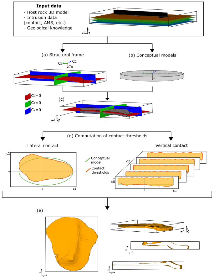
Figure 2Workflow for the proposed method using a synthetic example of a sill intrusion. The data and prior knowledge indicate that the sill exploits the host rock's bedding and two faults to step up in the stratigraphy. (a) The structural frame's coordinates are built using the following data: the geometry of the bedding and faults for coordinate 0, propagation data for coordinate 1, and synthetic vectors perpendicular to the sill's long axis for coordinate 2. (b) The conceptual models used are the ellipse and a constant function to constrain the lateral and vertical extent, respectively. (c) Conceptual models and structural frame observed along X–Y–Z axes. (d) Conceptual models (green lines) and conditioned conceptual models (orange lines) observed along the structural frame axes. (e) Different views of the isosurface that represents the intrusion contact.
3.2 Intrusion structural frame
The intrusion frame is built using LoopStructural implementation of structural frames (Grose et al., 2021a, b), in which the coordinates are interpolated sequentially using a discrete interpolator, e.g. finite-difference interpolation on a Cartesian grid (Irakarama et al., 2021) or piecewise linear interpolation on a tetrahedral mesh (Frank et al., 2005, 2007). These interpolation methods are mesh-based methods; therefore, the size of the mesh elements and the resolution of the mesh will impact the resulting 3D models.
The intrusion frame coordinates represent geometrical elements of the intrusion shape (Fig. 2a). The first coordinate (c0) measures the distance between the roof and floor contacts of the intrusion. Its scalar field is interpolated using contact observations and is constrained to be parallel to the host rock foliation and/or structures that facilitated the emplacement of the intrusion. Such mechanical anisotropies are defined by the modeller. The gradient of this coordinate's scalar field is forced to be perpendicular to the host rock's anisotropies, unless inflation measurements are available. The isosurface c0=0 approximates the location of the roof or floor contact (depending on the data used to constrain this coordinate). The second coordinate (c1) describes the propagation of the magma and is interpolated using measurements (or geological knowledge) of the propagation direction. The gradient of the c1 scalar field follows the direction of the magma propagation, and, conceptually, the isovalue c1=0 should be related to the position of the intrusion feeder. However, for the modelling, this isosurface can be anywhere in the model. The third coordinate (c2) measures the distance to the long axis of the intrusion. It is interpolated using points along the intrusion long axis and an additional constraint enforcing the orthogonality between the gradients of c1 and c2.
3.3 Conceptual models and threshold functions
The intrusion frame coordinates are used to parameterise two conceptual models that represent a simplified interpretation of the coarse-scale geometry of the intrusion (Fig. 2b). These conceptual models are simple geometric shapes observed along the frame coordinates; however, they may show a more complex geometry observed within the X–Y–Z coordinate system (Fig. 2c). The first conceptual model, ℭL(c1)=c2, returns a distance along c2 for any c1, and it represents the geometry of the intrusion lateral contact. The second conceptual model, , returns a distance along c0 for any (c1,c2), and it represents the geometry of the roof or floor contact of the intrusion, depending on which of these contacts were used to build the intrusion frame. For example, if the intrusion frame c0 is built using roof contact points, ℭV represents the geometry of the intrusion floor.
These conceptual models and their parameters are defined by the modeller. For example, to represent the lateral extent of an elongated sill segment, the modeller may choose the ellipse function as ℭL. The centre of the ellipse would be set to be the centre of the intrusion, and the length of the ellipse major and minor axes should be defined so the ellipse encloses the majority of the contact data.
To fit each of these models to the contact data (Fig. 2d), we propose the following steps for a set of roof or floor contact points pi with ; a set of lateral contact points pk with ; and their associated intrusion frame coordinates and , respectively.
Firstly, compute the residual values RV and RL between the data and the conceptual model at the data locations as follows:
Here, ℭV and ℭL are the geometrical conceptual model for the vertical and lateral contact, respectively. Secondly, use an exact interpolator to construct an interpolation function for both RV and RL. We call these interpolation functions and , respectively, and they will allow us to estimate the residual values away from the input data. Interpolating the residual values using an exact interpolator enables us to condition the model to the data at this step. However, other interpolation techniques can be used, and the model can be conditioned to the data afterwards. For all of the examples presented in Sect. 4, we have employed a linear radial basic interpolation.
Finally, distance threshold functions TV,L(p) are defined as the difference between the conceptual models ℭV and ℭL and the interpolation functions and .
These threshold functions TV,L(p) characterise the vertical and lateral contact of the intrusion along the structural frame coordinates. TV returns distances along c0 and provides the location of the roof (or floor) contact for any (c1,c2). TL returns a distance along c2 and represents the location of the side contacts of the intrusion for any c1.
Using the threshold functions along the intrusion frame coordinates, the intrusion body I can be defined as follows:
3.4 Implicit description of the intrusion geometry
The implicit description of the intrusion can be obtained by modifying the intrusion frame scalar fields, so the intrusion contact characterised by the threshold functions along the frame coordinates is represented by the isosurface zero of this modified scalar field (Fig. 2e). This can be achieved by different combinations of the scalar fields and threshold functions.
In this section, we present three case studies that show the applications of our approach to different types of intrusions: a sill complex, a pluton, and a laccolith. We also present a comparison between our method and radial basis function interpolation using an example of a sill complex offshore of Western Australia. These examples are presented as interactive Jupyter notebooks that can be downloaded from https://doi.org/10.5281/zenodo.10463777 (Alvarado-Neves, 2024).
4.1 Case study 1: synthetic sill complex
The first case study (CS1) is a synthetic sill complex composed of three sill segments. The sill complex is emplaced in a horizontal stratigraphic sequence, and the sill segments propagate to the north, with slightly different directions. Two of the sill segments (segments 0 and 1) were intruded at the same stratigraphic level, whereas the middle segment (segment 2) exploited a pre-existing east–west trending fault and stepped up in the stratigraphy.
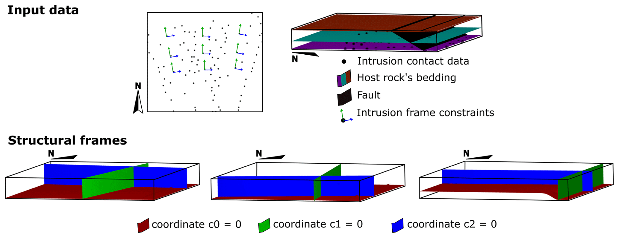
Figure 3Input data and structural frames of case study 1 – synthetic sill complex. The dataset consists of the 3D model of the host rock, roof and floor contact points, propagation data, and synthetic vectors perpendicular to the long axis of each sill.
In this example, the input data consisted of an implicit geological model of the stratigraphic sequence and the fault; contact data of the roof, floor, and sides of each sill segment; and propagation vectors and points located at the long axis of each segment. Figure 3 shows the 3D geological model of the host rock and the spatial distribution of the sill segments' data. The intrusion frame of each segment is built using the floor contact point and propagation and long-axis data (Fig. 3). The three sill segments are built with the same conceptual models: the ellipse equation as the lateral contact conceptual model ℭL and a constant function as the vertical conceptual model ℭV.
In the above expressions, (, ) is a point chosen arbitrarily in the centre of the intrusion considering the data spatial distribution; a, b, and c are the average of the c1, c2, and c0 coordinate values of the input data, respectively. Considering that c0= 0 approximates the location of the floor, ℭV is equivalent to the mean thickness of each sill. Figure 4 shows the 3D geological model of this case study. Sectional views along the y axis show structures usually developed in sill complexes, like broken bridges when sills inflate and coalesce or bridges when they inflate without coalescing.
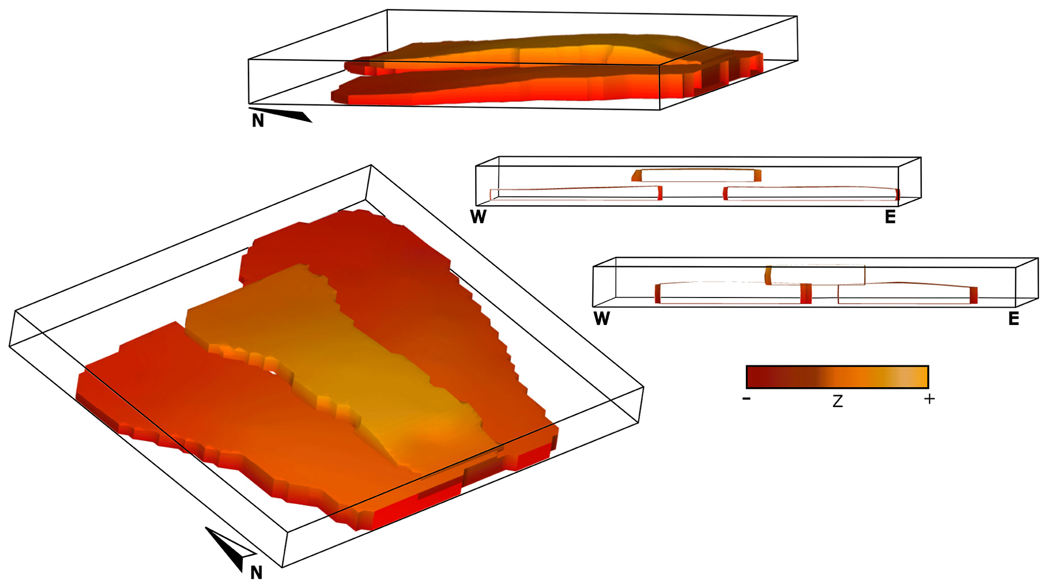
Figure 4Three-dimensional geological models of case study 1 – synthetic sill complex. To the right, two cross-sections show the bridge and broken bridge structures developed between the sill segments. The isosurfaces are painted with the elevation value at each location, highlighting the relief of the models.
4.2 Case study 2: Voisey's Bay intrusion
The second case study is the Voisey's Bay intrusion in Labrador, Canada. In this case study, we created the dataset by selecting intrusion contact data points from the geological map and geological cross-sections presented by Saumur and Cruden (2015). The floor data points were picked from the drill holes in the interpreted cross-sections. The roof and lateral data were picked from the geological map; therefore, it is assumed that the roof is located in the current topography. The host rock was modelled as a horizontally foliated unit. Figure 5 shows the 3D model of the host rock and the contact data points.
Considering the spatial distribution of the contact data, we approximate the long axis of the intrusion as a south-east–north-west line centred in the intrusion. The intrusion frame coordinate c0 is constrained using the roof contact data and is assumed to be parallel to the host rock foliation. The axis of coordinate c1 is constrained to be parallel to the long axis, and coordinate c2 perpendicular to the long axis. Figure 5 shows the intrusion frame of this case study.
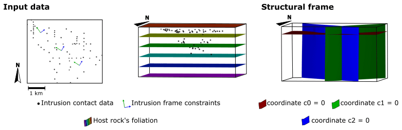
Figure 5Input data and structural frames of case study 2 – Voisey's Bay intrusion, Canada. The dataset consists of a 3D model of the host rock and roof and floor contact points extracted from the area's geological maps and cross-sections of the area. Synthetic data constrain coordinates 1 and 2 of the structural frame, which is coherent with the data spatial distribution.
To show the effects of the conceptual models on the results, we present two 3D geological models of the Voisey's Bay intrusion, each of them constrained with a different conceptual model of its floor geometry. Both models are constrained using the ellipse equation as the lateral contact conceptual model ℭL, similar to the previous case study (Sect. 4.1). Model A is constrained using the equation of an oblique cone as ℭV, while model B is constrained using a constant function.
In the above expressions, is the conic guiding curve of the cone, and represents the intrusion frame coordinates of the deepest data point, which acts as the vertex of the cone in model A. Figure 6 shows the resulting 3D models.
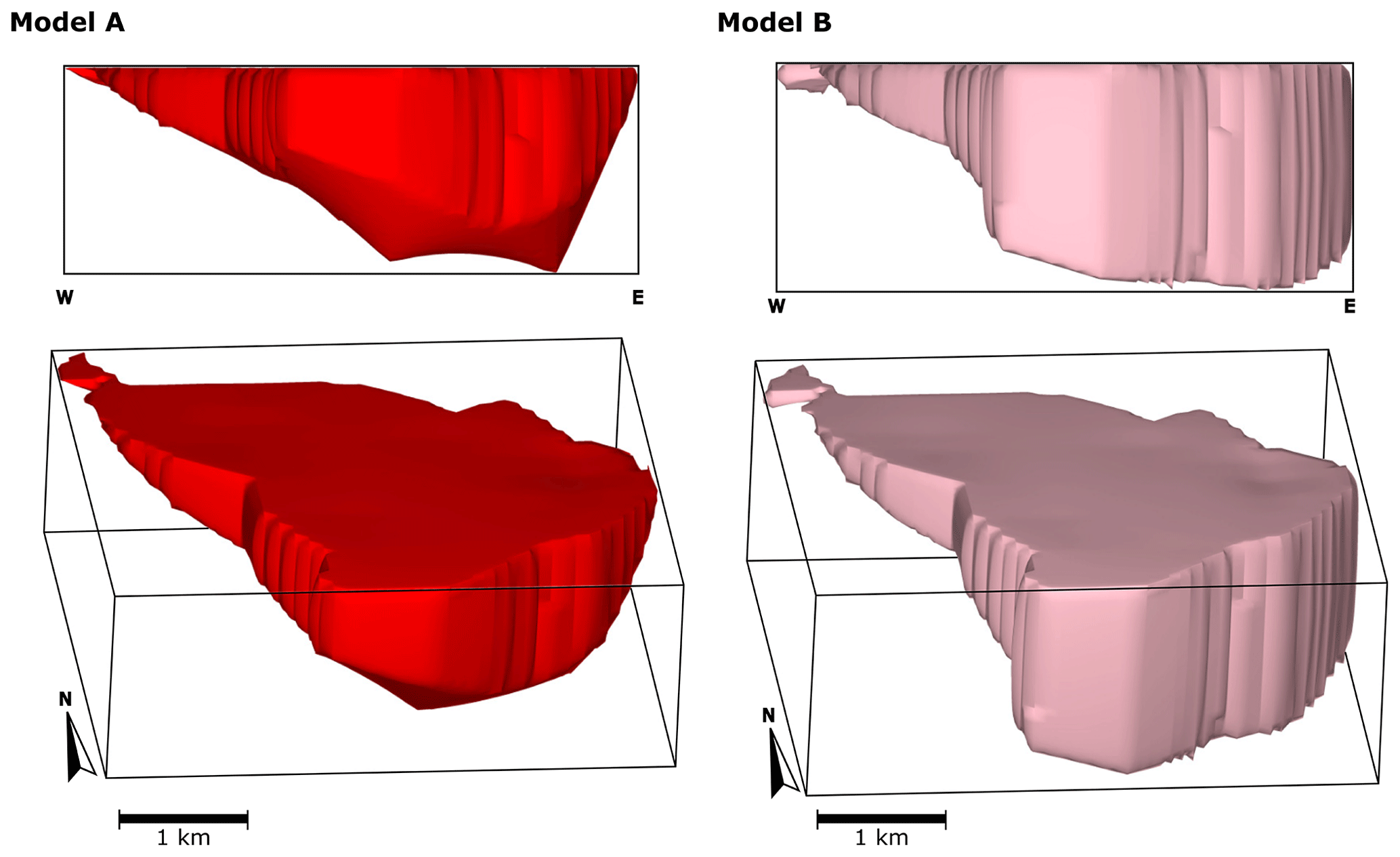
Figure 6Three-dimensional geological models of case study 2 – Voisey's Bay intrusion, Canada. Models A and B are built using the same input data and the ellipse function to constrain their lateral contact. The difference between them is the function that limits their vertical contact. Model A is constrained using the cone function, whereas model B is constrained using a constant function.
4.3 Case study 3: synthetic laccolith
The third case study is a synthetic laccolith emplaced in a horizontal stratigraphic sequence. The input data consisted of an implicit geological model of the stratigraphy, six data points of the roof and floor contact of the intrusion, and a point in the middle of the intrusion that indicates the laccolith long axis' position and a propagation direction parallel to the long axis. The intrusion frame is built using the floor contact, propagation and long-axis data, and its coordinate zero is constrained to be parallel to the host rock bedding. Figure 7 shows the 3D geological model of the host rock, the distribution of the laccolith data, and the intrusion frame.
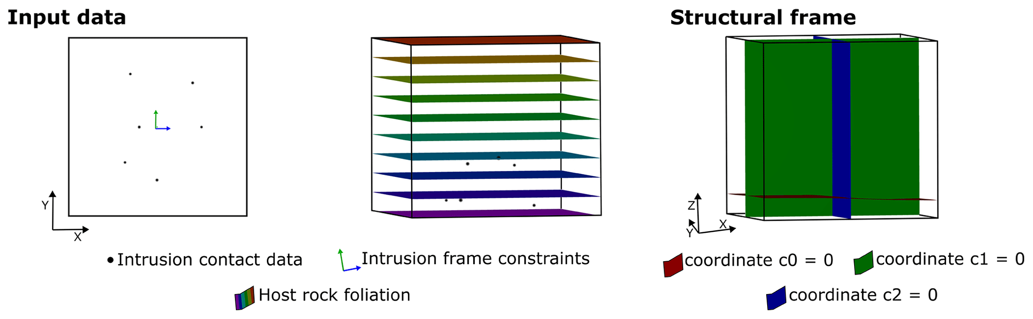
Figure 7Input data and structural frames of case study 3 – synthetic laccolith. The dataset consists of the 3D model of the host rock, six roof and floor contact points, and one point and vector to constrain coordinates 1 and 2 of the structural frame.
The conceptual models used in this example are the ellipse equation as the lateral contact conceptual model ℭL (same as case studies 1 and 2) and a bell curve function as the vertical conceptual model ℭV.
Here, a is the maximum half-distance between the data points along c1 and b is the middle point along c1, considering the spatial distribution of the data.
The threshold function TV characterises the thickness variation in the intrusion as distances along c0 for any (c1,c2). To reproduce the effects of the intrusion emplacement by roof lifting into the host rock, we use TV to modify the geometry of the horizontal stratigraphy, so it is concordant with the intrusion roof. We defined the post-intrusion stratigraphy smod(p) as follows:
Here, s(p) is the scalar field defined to characterise the pre-intrusion stratigraphy; TV(p) is the threshold function that represents the distance between the roof and floor of the laccolith, which is a proxy for the intrusion thickness; and I is the intrusion body given by Eq. (3). Figure 8 shows the resulting 3D model as well as a cross-section of the model illustrating the geometry of the host rock after the emplacement of the intrusion.
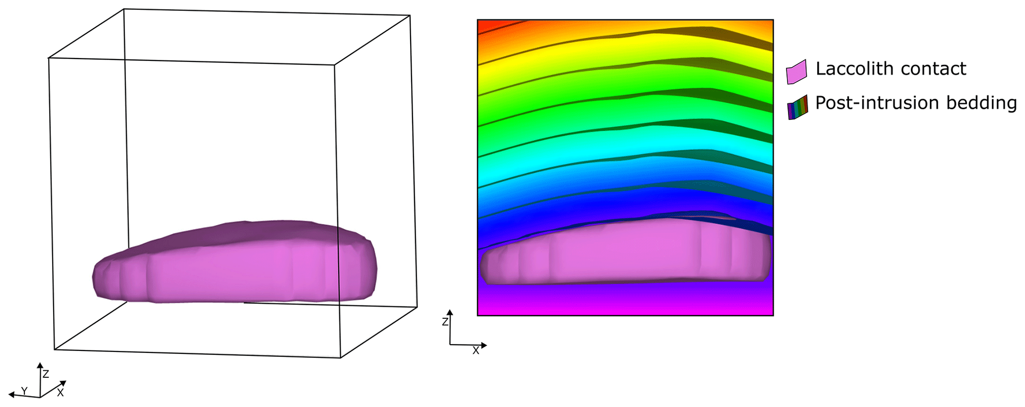
Figure 8Three-dimensional geological model of case study 3 – synthetic laccolith. To the right, a cross-section shows the geometry of the bedding folded using the geometry of the laccolith roof.
4.4 Comparison with radial basis function interpolation
Radial basis function (RBF) interpolation is one of the main approaches currently used to build implicit 3D geological models (Hillier et al., 2014; Cowan et al., 2002; Wellman and Caumon, 2018). To assess the value of our approach, we present a comparison between our method and radial basic function interpolation. We apply both methods to build 3D geological models of a sill intrusion in the offshore north-western Australia shelf (case study 4; Köpping et al., 2022). This real-world case study is an exceptional example to perform the comparison, as it has been extensively mapped with respect to seismic images and its geometry is well characterised. We built four 3D geological modes for this case study, whose differences arise from the method used to build them and the number and type of input data. Models A and B are built using radial basic function interpolation and differ with respect to the number of input constraints for each model. Models C and D are built using our proposed method, and the difference between them is that model D incorporates geometrical constraints from the emplacement history proposed by Köpping et al. (2022).
The input contact data for the models comprise a randomly selected sample of the dataset presented by Köpping et al. (2022). The original dataset consists of the sill base and top contact points picked from seismic imagery and covers approximately 4042 km2 with >2.5 million data points (Fig. 9a). According to Köpping et al. (2022) and our Fig. 9, the intrusion is composed of a 13.4 km long, north-trending, strata-concordant inner sill that transitions into transgressive inward-dipping inclined sheets along its eastern margin and south-western margin. Where inclined sheets are developed, the horizontal dimension of the inner sill is relatively narrow (∼3.4 km). In the northern section of the sill, where no inclined sheet has developed on the western margin, the inner sill widens up to 6.4 km and has a convex-outwards and lobate western termination. The authors present a detailed characterisation of the vertical thickness variation within the sill (Fig. 9b). The eastern half of the inner sill is ∼166 to ∼249 m thick, rapidly decreasing westward to ∼111 to ∼166 m. The inclined sheets, the southern sill tip, and the north-western lobate termination are presented as tuned reflection packages, and their thickness can only be defined by the limits of separability and visibility of the data (∼7 to ∼56 m).
Köpping et al. (2022) propose an emplacement model for the sill, as schematically represented in Fig. 9c. The sill comprises one segment that propagated and inflated northward from a south-west–north-east-trending fault and another segment that propagated to the south-west of this fault. This south-west–north-east-trending structure is located in the middle of the sill and likely also facilitated magma ascent. The transgressive inward-dipping inclined sheets formed along pre-existing faults in the east and south-west. The straight geometry of the south-western limb is interpreted to be controlled by pre-existing fractures and/or faults.
The preprocessing of the data, the workflow, and the results of the four models are presented in the following subsections. The input data are presented in Fig. 9 and the resulting 3D models are presented in Fig. 10.
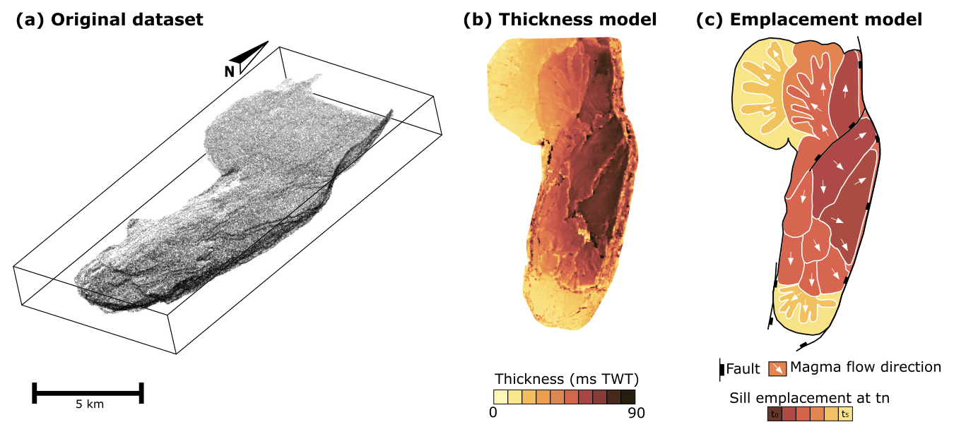
Figure 9Data and models of Köpping et al. (2022): (a) top and base contact points picked on seismic images, (b) two-way time thickness model, and (c) schematic diagram of the emplacement history of the sill.
4.4.1 Models A and B - radial basis function (RBF) implicit interpolation
Models A and B were built using the “SurfE” interpolator available in LoopStructural (Grose et al., 2021, b). SurfE (https://github.com/MichaelHillier/surfe, last access: 29 February 2024) implements a generalised radial basis function interpolator (Hillier et al., 2014). Radial basis function interpolation is a meshless interpolation method where the scalar field is constrained with different types of data, including value and gradient constraints. Models A and B are built using the signed distance interpolation of SurfE (single-surface method).
The input data for these models consist of value and gradient constraints (Fig. 10). In both models, the value constraints represent the intrusion contact location, and a value of zero is assigned to each of these points. The gradient constraints employed for these models are vectors perpendicular to the stratigraphy with a direction towards the outside of the intrusion. These data are equivalent to the polarity constraint (e.g. Calcagno et al., 2008) and are synthetic data which are required to interpolate the scalar field with RBF. For model A, a randomly selected subsample of approximately 0.1 % of the original dataset is used as value constraints, and a selection of these points located in the strata-concordant inner sill are used as gradient constraints. For model B, we increase the amount of value and gradient constraints to approximately 0.5 % of the original dataset, with the gradient constraints distributed within the inner and outer sills.
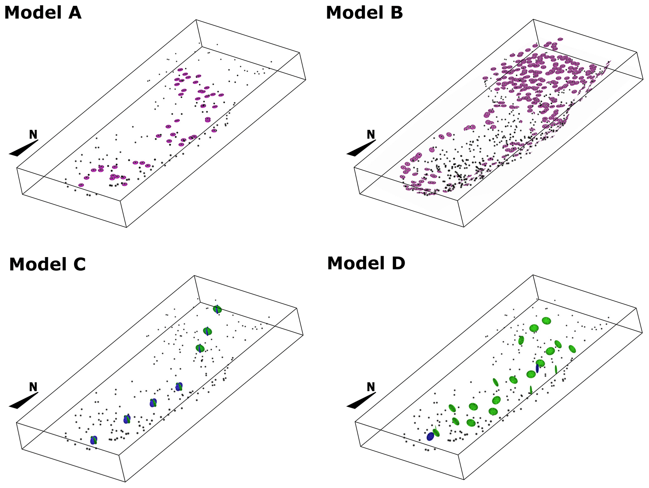
Figure 10Case study 4 – sill complex in Western Australia. The figure shows the spatial distribution of point data employed to build the models. In all of the models, black dots represent the location of intrusion contact data. In models A and B, pink circles represent the locations of gradient constraints. In models C and D, green and blue circles represent the gradient constraints for coordinates 1 and 2 of the structural frame, respectively. All circles are facing towards the direction of the gradient constraint.
4.4.2 Models C and D - structural frame and conceptual models
Models C and D are built using the approach introduced in this work. The main difference between these two models is that model D integrates geometrical constraints from the sill emplacement history proposed by Köpping et al. (2022). In other words, we use the geometry of the faults that facilitated the emplacement of the transgressive sills and the conceptual propagation model proposed by Köpping et al. (2022). The resulting 3D models are shown in Fig. 10.
The contact data for both models consist of a sample of approximately 0.1 % of the original dataset – the same data points used for model A. These points are classified as top, base, and lateral contacts depending on their location. For model C, the intrusion frame c0 is built using the sill's base contact points and is constrained to be perpendicular to the host rock. To constrain coordinates c1 and c2, we approximate the long axis of the intrusion considering the spatial distribution of the data. The gradients of c1 and c2 are constrained to be parallel and perpendicular to the long axis, respectively (Fig. 10).
For model D, we consider the sill composed of two segments emplaced at opposite sides of a north-east–south-west-striking fault (Fig. 10; Köpping et al., 2022). The northern segment propagates into the fault's hanging wall towards the north-north-west, and its geometry is controlled by the eastern marginal fault generating a transgressive sill. The southern segment propagates within the footwall towards the south-east and then south-south-west. The transgressive sills to the east and west of the southern segment are controlled by pre-existing faults. The two segments are modelled separately. For both segments, the intrusion frame c0 is built using the sills' base contact points and is constrained to be parallel to the host rock and the marginal faults involved in their emplacement. The propagation vectors given by the emplacement model of Köpping et al. (2022) are used to constrain c1, and c2 is constrained using a point located in the middle of the sill with its gradient enforced to be perpendicular to c1 (Fig. 10).
Models C and D are built with the same conceptual models: the ellipse equation as the lateral contact conceptual model ℭL and a constant function as the vertical conceptual model ℭV. ℭV is equal to the mean thickness of the sill given by the input data.
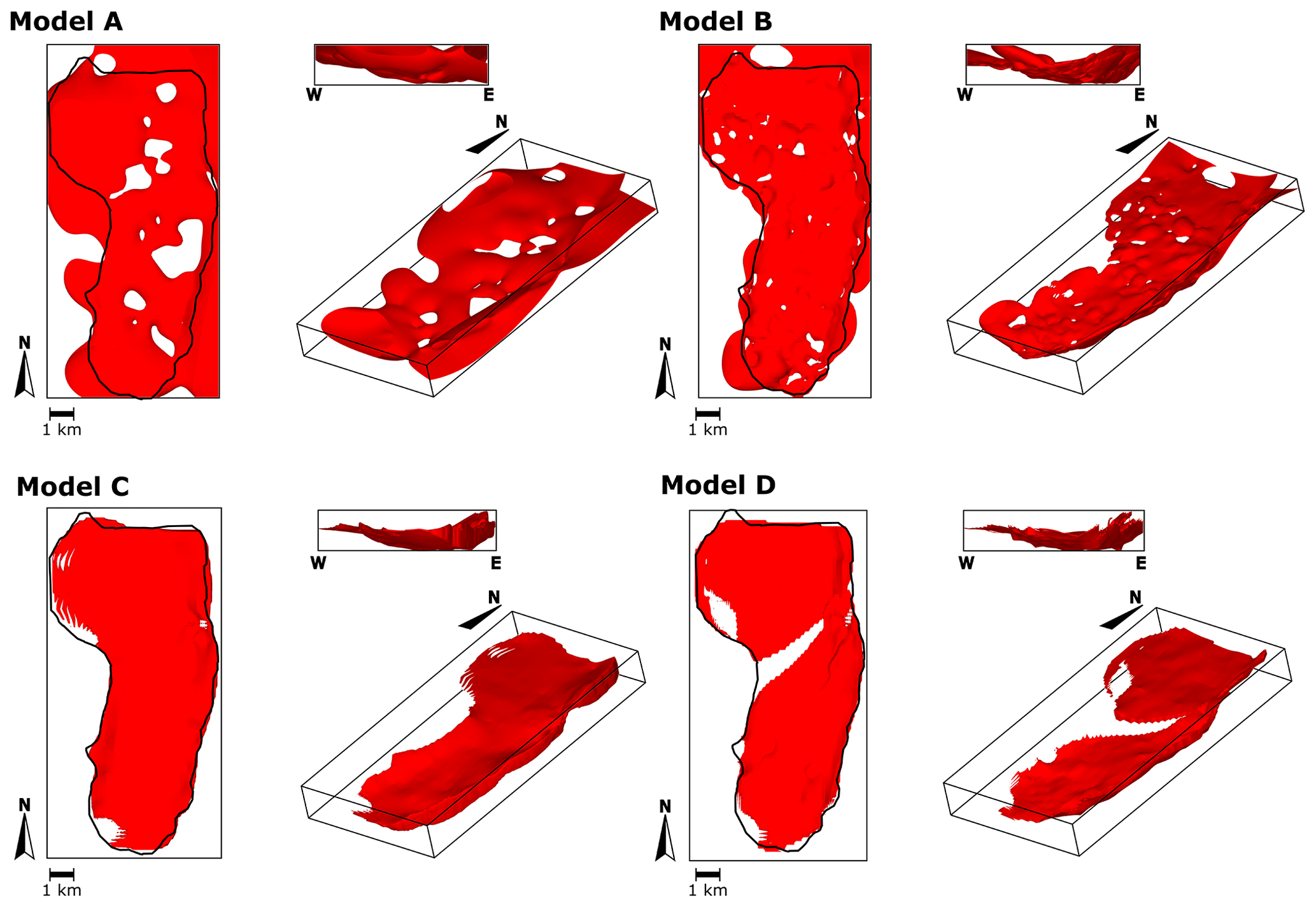
Figure 11Three-dimensional geological models of case study 4 – sill complex in Western Australia. Models A and B were built using radial basis function interpolation, whereas models C and D were built using the method proposed in this work. Black lines indicate the contour of the sill mapped in seismic images by Köpping et al. (2022).
4.4.3 Comparison between the models
The resulting 3D models are presented in Fig. 11. The grid employed for visualisation of the models has elements, and each element has a size of 74 m × 150 m ×8 m. Visual inspection shows that, in general, RBF interpolation and our method can reproduce the coarse-scale geometry of the sill, with a north-trending inner sill transitioning to inward-dipping outer sills. Considering the geometric description provided by Köpping et al. (2022) and our Fig. 9, our method is more accurate at constraining the shape of the terminations of the sill, whereas the RBF interpolation extrapolates the isosurface that represents the intrusion contact away from the data. This is exacerbated in model A due to the reduced number of input data compared with model B. In RBF interpolation, the value of the basis function depends on the distance ∥x−xi∥, where x is the position to evaluate the function and xi is the location of the data point, which may generate blobby geometries away from the data (Wellmann and Caumon, 2018). Models A and B present holes within the intrusion related to the absence of on-contact or planar constraints. Models C and D do not capture some of the thinnest parts of the sill, such as the southern tip, the north-western lobate termination, and the eastern inclined sheet of the northern segment and next to the feeder fault of model D. In these areas, the grid elements have larger dimensions than the width or length of the modelled sill; therefore, the isosurface representing the intrusion contact is not captured in the scalar field values assigned to each of the grid nodes.
To assess how realistic the resulting 3D models are, we compare the geometry given by the seismic imagery and the geometry given by each model. We visually inspect 12 cross-sections and measure each model's thickness. As an example, Fig. 11 shows one cross-section along the x axis and one cross-section along the y axis. Model A shows substantial differences compared with the other models, and it does not reproduce the expected sheet-like shape of a sill nor a clear transition from the inner to the outer sill. Models B, C, and D capture the inclined geometry of the outer sills; however, model C seems to flatten the eastern inclined sheet. This is because model C's intrusion frame is interpolated using the base contact points, and this interpolation does not necessarily capture the geometry of the faults that control the transgressive sill. Models C and D are slightly better at recovering the straight top and base contacts, while model B exhibits wavy contacts in some parts of the model.
The thickness of the models is measured in predefined locations and compared with the thickness given by the seismic imagery observations. Figure 12 shows the location of the measurements and the thickness contours interpolated using these measurements of each of the models. As Köpping et al. (2022) describe, their data show that the intrusion thickness decreases from east to west within the inner sill and towards the tips and inclined outer sills. Model A does not show any evident trend, and the thickness is generally larger than the thickness given by the data. Model B thins down towards the western lobate termination but does not capture the decreased thickness observed in the outer sills and the southern tip. Models C and D show a decreasing trend towards the western and southern tips but tend to amplify the difference with the data closer to the outer sills. We compute the absolute difference between the thicknesses measured on each model and the thickness given by the data (Fig. 12, Table 1). This difference's mean and standard deviation are significantly lower in model B compared with model A, showing the effect of adding more constraints to the RBF interpolation. Model C and D have a similar mean and standard deviation, and these figures are slightly lower in model C. Even though models C and D show less difference with the thickness measured in seismic images by Köpping et al. (2022), there are areas of these models where the thickness difference is significantly large. This is observed closer to the eastern marginal fault, and it stems from the fact that the geometry of c0 does not entirely capture the sharp transition between the inner and outer sills. This smoother transition can also be observed in the cross-sections presented in Fig. 12.
Table 1Input data and results of the thickness comparison between the models of case study 4.
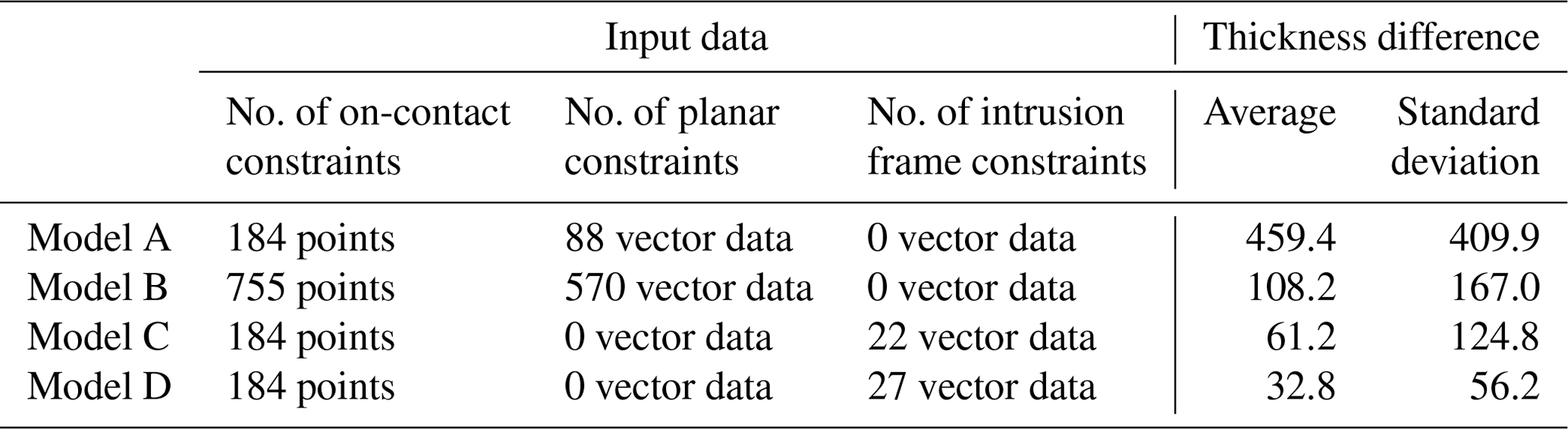
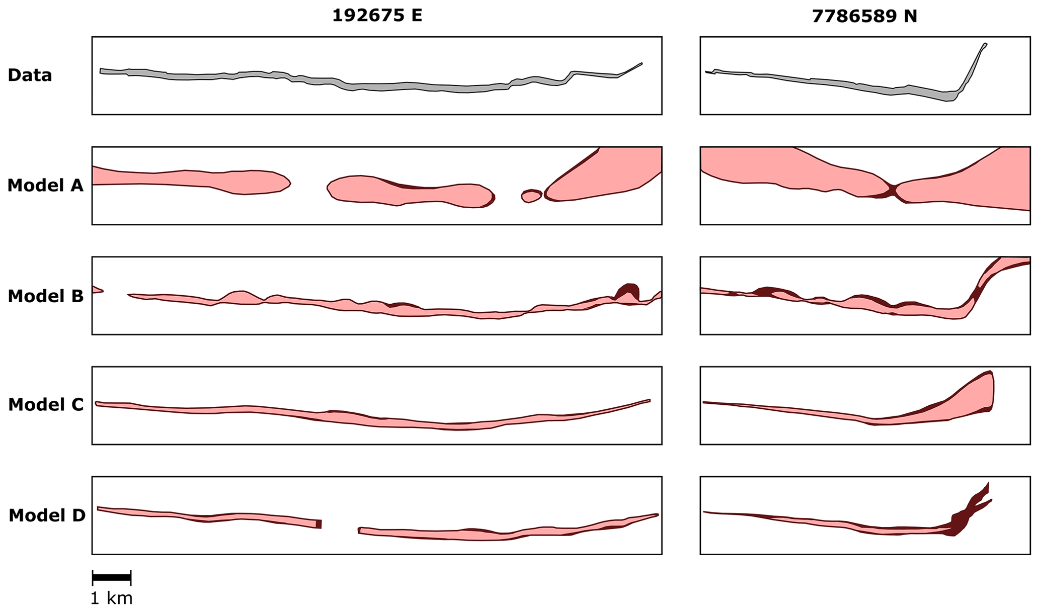
Figure 12Assessment of the 3D geological models of case study 4 – sill complex in Western Australia. The figure shows cross-sections of the models along 192675 E and 7786589 N (UTM WGS84 Zone 50S). Models A and B were built using radial basis function interpolation, whereas models C and D were built using the method proposed in this work. The first row of polygons (data) shows the area enclosed by the dataset presented by Köpping et al. (2022) and shown in our Fig. 9.
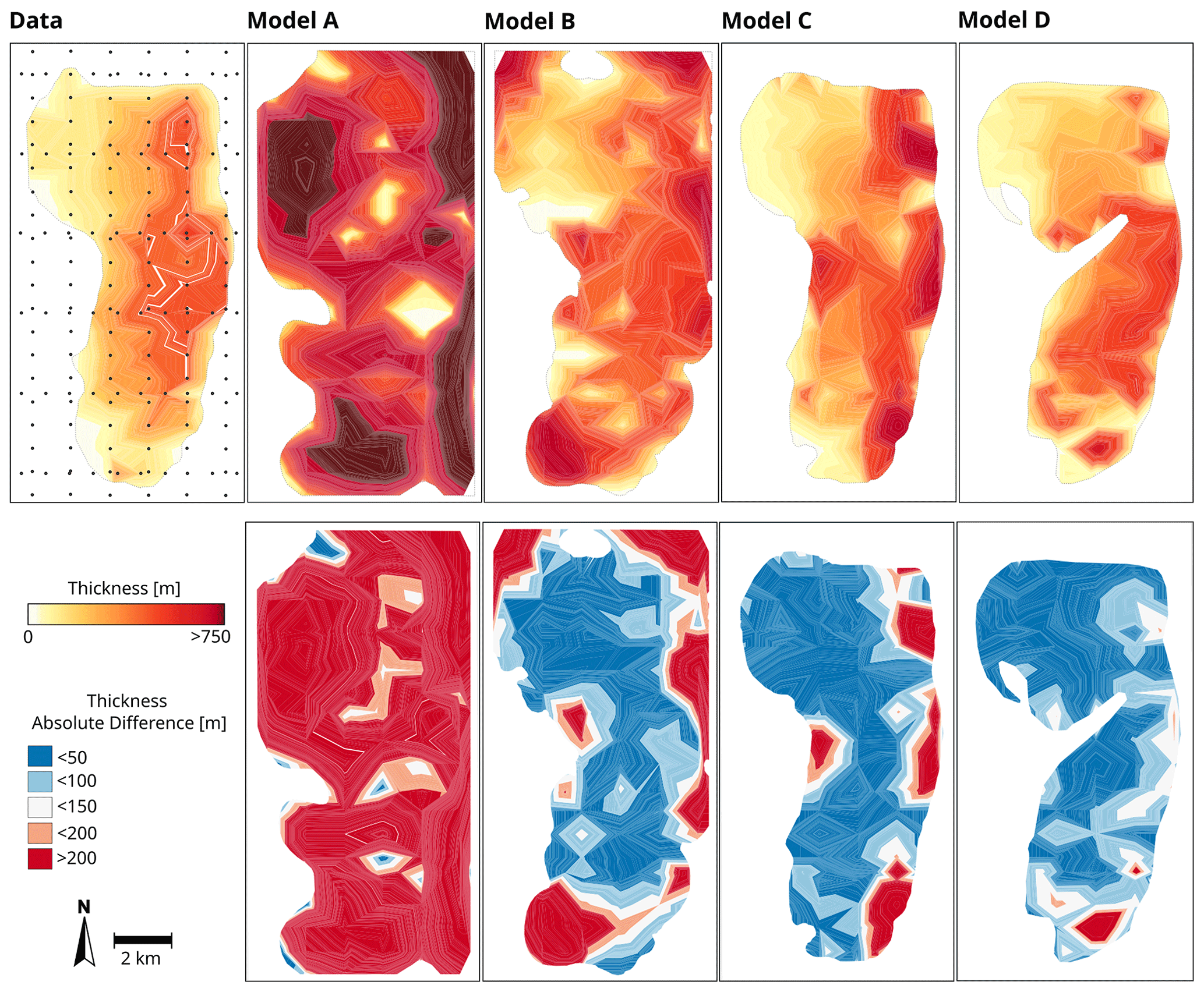
Figure 13Assessment of the 3D geological models of case study 4 – sill complex in Western Australia. The figure compares the models' thicknesses (first row) and the absolute difference between the thickness given by the data and the thickness given by the models (second row). Models A and B were built using radial basis function interpolation, whereas models C and D were built using the method proposed in this work. The panel to the left (data) shows the location of the thickness measurements and thickness contours estimated using the thickness data of Köpping et al. (2022). The other panels show thickness and thickness difference contours estimated using the measurements from each model. The estimated contours are clipped using the outline of each model.
To date, 3D models of intrusions have been built with classical interpolation workflows, in which on-contact data and a polarity constraint indicating the inside/outside of the intrusion are used to estimate the contact. Post-processing is usually required to generate the intrusion shapes observed in the field, drilling data, or imaged in geophysical surveys, making the model dependent on the modeller's expertise and challenging to reproduce. In this contribution, we address these limitations by implementing a method inspired by the object-distance simulation method (Henrion et al., 2008, 2010) and that uses an adapted structural frame for intrusions (Laurent et al., 2013, 2016; Godefroy et al., 2017; Grose et al., 2021a, b). The models can be constrained with contact data and other field measurements such as inflation direction and propagation direction.
The structural frame incorporates conceptual knowledge of intrusion emplacement mechanisms into the modelling framework. This is achieved by constraining the structural frame with the geometry of the foliation or geological structures that facilitated the emplacement of the intrusion. Thus, the geometry of the modelled intrusions is controlled by the geometry of the host rock. It may also be constrained using the inflation and propagation direction, if these data or this conceptual knowledge is available. The intrusion frame allows one to characterise the geometry of intrusions more simply. For example, a saucer-shaped (e.g. CS4) sill becomes a straight, tablet-shaped sill viewed along the coordinates of the intrusion frame. This is particularly useful for complex systems of intrusions, such as sills that step up and down within the stratigraphy with variable propagation directions.
One limitation of constraining the structural frame with host rock anisotropies is that, in theory, the method could be only applicable to intrusions whose emplacement was controlled by mechanical anisotropies. However, in practice, as long as the modeller knows the coarse-scale geometry of the intrusion, this can be overcome by setting the directions of the structural frame coordinates to follow the major direction of the intrusion. This is demonstrated in CS2 (Voisey's Bay intrusion), in which the emplacement mechanism is unknown. The contact data suggest an intrusion whose roof is roughly horizontal; therefore, we set up the structural frame to follow the orientation of a synthetic horizontal foliation. This is done because the current implementation of the method requires defining at least one mechanical anisotropy to constrain the geometry of the structural frame. We suggest that the next iteration of the method implementation should remove this requirement, which would add flexibility to constrain the structural frame without changing the essence of the proposed method.
The intrusion frame coordinates are employed to parameterise conceptual models that represent the coarse-scale geometry of the intrusion. The conceptual models represent a parametric description of the intrusion thickness and width, and the modeller defines these functions. They would be comparable to defining a conceptual model while drawing shapes or adding arbitrary (not quantified through proper geostatistical analysis) structural trends to the model, although with no manual processing. Thus, the conceptual models allow one to build objective and unbiased 3D models considering prior knowledge of the intrusion geometry. While the method workflow accepts any parametric function, it is recommended that these functions agree with the geometries observed in reality (see Sect. 2). The appropriate function can be selected after assessing the data and the regional context. The conceptual models also allow one to test different scenarios. In CS2, we create two models of the Voisey's Bay intrusion that differ with respect to the conceptual model. In one of them, we model a scenario where the intrusion has a wedge-shaped geometry using the function of an oblique cone to constrain the intrusion floor geometry. In the second model, we test a tablet-shaped geometry using a constant function to constrain the floor geometry. Both models comprise two alternatives for the geometry of the intrusion considering the spatial distribution of the data. A workflow to automatically find the best-fitting conceptual model can be implemented in the future. Following the approach of Grose et al. (2018, 2019), fitting the conceptual model to the observations can be considered to be an inverse problem. Finally, the conceptual models allow one to build intrusion models with small contact datasets and in the absence of lateral data, as shown in case study 3.
The structural frame and the conceptual model allow us to have an implicit representation of the intrusion thickness and width within the intrusion extent. This implicit representation can be used to modify the host rock to recreate the effects of the intrusion emplacement in the host rock geometry. This is demonstrated in case study 3, where we modify the originally flat-lying host rock to obtain a folded bedding concordant with the bell-shaped geometry of the laccolith roof. Further work should consider demonstrating this capability using real-world case studies.
The proposed method and its implementation allow one to add conceptual knowledge of the intrusion emplacement history and its morphology via the structural frame and conceptual models. Even though this could make the models strongly conceptual (such as CS3), the data that our method employs carry geological significance and can be interpreted in a geological context. This is a significant difference compared with existing interpolation approaches to build intrusions 3D models, which are required to have a gradient constraint that lacks any geological meaning.
In general, the 3D models of the four case studies presented in this work are in good agreement with the intrusion geometries described in the literature (e.g. Cruden et al., 2017, 1999; Galland et al., 2018; Jackson et al., 2013; Kavanagh, 2018; McCaffrey and Petford, 1997; Vigneresse, 1995; Vigneresse et al., 1999). These examples demonstrate the capability of our method to reproduce intrusion geometries, in particular, the coarse-scale geometry of sill segments and the connectors developed after the interaction between sill segments in a sill complex; the coarse-scale geometry of plutons, with a roughly flat roof with a symmetric or asymmetric floor; and the bell-shaped geometry of laccolith. The examples also show that the method can create realistic intrusion shapes considering small datasets from surface or drilling data. The modelling workflow for other intrusion types, such as dykes or lopoliths, would be similar, with the main difference being the conceptual model defined for each case.
Considering our case study 4 (Sect. 4.4), our method can more truthfully reproduce the sill geometries imaged in seismic surveys, compared with RBF interpolation. In particular, our method can replicate the sheet-like geometry of this sill intrusion, constrain its terminations and thickness variations, and generate a model of similar dimension, including thickness variation trends, to what is observed in contact data. Parameterisation of the intrusion using the structural frame is crucial and enables a rigorous computation of the intrusion extent in the direction in which the intrusion grew. This parameterisation enables the modeller to incorporate geometrical constraints based on the emplacement history of the intrusion, as we did in model D. However, the current implementation of the method is limited with respect to accurately capturing the sharp transition between the inner and outer sills, which results in large differences in thickness on the eastern side of the sill (Fig. 13). This could be refined by improving how the structural frame is enforced to be parallel to the host rock anisotropies involved in the intrusion emplacement.
One of the advantages of our approach over RBF is that the modeller can add geometrical constraints based on the emplacement history of the intrusion. For case study 4, we model the transition between the inner and outer sill using the geometry of the marginal faults in model D. This type of geometry would be difficult to reproduce using a classic interpolation approach unless a large dataset was provided, as in model B. However, having a dense dataset is rarely the case, and models of intrusions are usually built using sparse and unevenly distributed datasets. The models built using RBF interpolation may be improved by modifying the distance scalar field with an elliptical conceptual model. Nevertheless, this is outside the scope of this work.
The computing time of adding an intrusion to the 3D models ranges from 3 to 20 s. The computing time is proportional to the size of the grid and the number of geological features (e.g. bedding and faults) used to constraint the intrusion frame. The computing time of building the 3D geological models presented in this work, including their visualisation, ranges from 15 s to 3 min. All of the models were built on a consumer laptop PC.
The method has two main limitations. The first one is that it does not employ off-contact data (i.e. inside or outside the intrusion) to constrain the models. This is a significant limitation considering that many observations are from within the intrusion and that their location is usually available. We suggest that this should be considered in further implementations, and it could be implemented in the definition and fitting of the conceptual models using inequality constraints. The second limitation of the method is that the surface representing the intrusion contact depends on the size of the model grid elements. Consider a part of the intrusion that is narrower or thinner than the size of a grid element; in this case, the nodes around the intrusion will indicate threshold values TV and TL smaller than their respective c2 and c0 coordinates, and they will not be indicated as being inside the intrusion. The scalar field value on these nodes will be greater than zero; therefore, no isosurface zero will be found between them. This scenario is observed in the narrower zone of the Voisey's Bay intrusion model (CS2; Fig. 6). According to the data, the intrusion transitions to a narrow and thin sill-like intrusion, which the model does not capture. This is also observed in the thinnest parts of the sill intrusion in north-western Australia presented in Sect. 4.4 (CS4, models C and D; Fig. 10). This limitation can be addressed using a higher-resolution mesh; however, this introduces computing limitations (time and memory usage). Adaptive-mesh algorithms should also be considered in the next iteration of the implementation.
Current methods to build 3D models of igneous intrusions are strongly dependent on data availability and manual processing. They do not consider geological knowledge of intrusion emplacement mechanisms objectively and do not use all types of measurements collected in the field. In this context, the generation of intrusion shapes observed in the field and in geophysics imagery is challenging to reproduce. To address these problems, we developed a method to build 3D models of intrusions that accounts for geological knowledge on intrusion emplacement mechanisms and typical datasets. The method is inspired by the object-distance simulation method (ODSIM) and incorporates an intrusion structural frame into the ODSIM framework that accounts for intrusion growth and propagation. This structural frame provides a curvilinear coordinate system for each intrusion within the model. Conceptual models of the intrusion contacts are parameterised using the structural frame coordinates and then fitted to the data. The conceptual models include a conceptual idea of the intrusion shape objectively and allow one to test different scenarios without the modeller's bias. The intrusion and the conceptual model provide a characterisation of the intrusion thickness and width that may be used to alter the host rock to 3D model the deformation associated with the intrusion emplacement. Fitting of all the data is not always feasible and may be dependent on the grid size. Further work on the method will include automatically fitting the conceptual models to the data, incorporating off-contact data, and employing adaptive meshes to improve the intrusion resolution.
The examples presented in this contribution were generated using the open-source 3D modelling package LoopStructural. LoopStructural v.1.5.10 can be downloaded from https://doi.org/10.5281/zenodo.7734926 (Grose et al., 2023) or installed using pip install LoopStructural. The input data and Jupyter notebooks of all the examples presented in this work can be downloaded from https://doi.org/10.5281/zenodo.10463777 (Alvarado-Neves, 2024).
All authors contributed to the conceptual design of the method and comparative analyses presented in this work. FAN developed the model code with editing and improvement contributions from LG. FAN prepared the manuscript with editing and reviewing contributions from all co-authors.
The contact author has declared that none of the authors has any competing interests.
Publisher's note: Copernicus Publications remains neutral with regard to jurisdictional claims made in the text, published maps, institutional affiliations, or any other geographical representation in this paper. While Copernicus Publications makes every effort to include appropriate place names, the final responsibility lies with the authors.
The authors thank Gautier Laurent and an anonymous reviewer for their insightful comments. The authors would like to also thank Jonas Köpping for providing the data for case study 4.
This research has been supported by the Australian Research Council (grant no. LP17010985 – Enabling 3D Stochastic Geological Modelling).
This paper was edited by Mauro Cacace and reviewed by Gautier Laurent and one anonymous referee.
Alvarado-Neves, F.: Fer071989/loopstructural_intrusions_gmd_ paper2023: LS Intrusion GMD paper, Zenodo [data set], https://doi.org/10.5281/zenodo.10463777, 2024.
Annen, C., Blundy, J. D., Leuthold, J., and Sparks, R. S. J.: Construction and evolution of igneous bodies: Towards an integrated perspective of crustal magmatism, Lithos, 230, 206–221, https://doi.org/10.1016/j.lithos.2015.05.008, 2015.
Barnett, Z. A. and Gudmundsson, A.: Numerical modelling of dykes deflected into sills to form a magma chamber, J. Volcanol. Geotherm. Res., 281, 1–11, https://doi.org/10.1016/j.jvolgeores.2014.05.018, 2014.
Braga, F. C. S., Rosiere, C. A., Santos, J. O. S., Hagemann, S. G., and Salles, P. V.: Depicting the 3D geometry of ore bodies using implicit lithological modeling: An example from the Horto-Baratinha iron deposit, Guanhães block, MG, REM – Int. Eng. J., 72, 435–443, https://doi.org/10.1590/0370-44672018720167, 2019.
Brown, M.: Crustal melting and melt extraction, ascent and emplacement in orogens: mechanisms and consequences, J. Geol. Soc. London., 164, 709–730, https://doi.org/10.1144/0016-76492006-171, 2007.
Brun, J. P. and Pons, J.: Strain patterns of pluton emplacement in a crust undergoing non-coaxial deformation, Sierra Morena, Southern Spain, J. Struct. Geol., 3, 219–229, https://doi.org/10.1016/0191-8141(81)90018-3, 1981.
Burchardt, S.: Introduction to volcanic and igneous plumbing systems-developing a discipline and common concepts, Elsevier Inc., 1–12 pp., https://doi.org/10.1016/B978-0-12-809749-6.00001-7, 2018.
Calcagno, P., Chilès, J. P., Courrioux, G., and Guillen, A.: Geological modelling from field data and geological knowledge: Part I. Modelling method coupling 3D potential-field interpolation and geological rules, Phys. Earth Planet. In., 171, 147–157, https://doi.org/10.1016/j.pepi.2008.06.013, 2008.
Cervantes, C. A.: 3D Modelling of Faulting and Intrusion of the Nevado del Ruiz Volcano, Colombia, Reykjavík University, 2019.
Chen, Y. and Nabelek, P. I.: The influences of incremental pluton growth on magma crystallinity and aureole rheology: numerical modeling of growth of the Papoose Flat pluton, California, Contrib. Mineral. Petrol., 172, 89, https://doi.org/10.1007/s00410-017-1405-6, 2017.
Clemens, J. D. and Mawer, C. K.: Granitic magma transport by fracture propagation, Tectonophysics, 204, 339–360, https://doi.org/10.1016/0040-1951(92)90316-X, 1992.
Cowan, E. J., Beatson, R. K., Fright, W. R., McLennan, T. J., and Mitchell, T. J.: Rapid geological modelling. International Symposium, Kalgoorlie, 23–25 September 2024, 2002.
Cruden, A. R.: On the emplacement of tabular granites, J. Geol. Soc. London., 155, 853–862, https://doi.org/10.1144/gsjgs.155.5.0853, 1998.
Cruden, A. R.: Emplacement and growth of plutons: implications for rates of melting and mass transfer in continental crust, in: Evolution and Differentiation of the Continental Crust, edited by: Michael Brown, T. R., Cambridge University Press, Cambridge UK, 455–519, 2006.
Cruden, A. R. and McCaffrey, K. J. W.: Growth of plutons by floor subsidence: implications for rates of emplacement, intrusion spacing and melt-extraction mechanisms, Phys. Chem. Earth A, 26, 303–315, https://doi.org/10.1016/S1464-1895(01)00060-6, 2001.
Cruden, A. R. and Weinberg, R. F.: Mechanisms of Magma Transport and Storage in the Lower and Middle Crust – Magma Segregation, Ascent and Emplacement, in: Volcanic and Igneous Plumbing Systems, Elsevier, 13–53, https://doi.org/10.1016/B978-0-12-809749-6.00002-9, 2018.
Cruden, A. R., Sjöström, H., and Aaro, S.: Structure and geophysics of the Gåsborn granite, central Sweden: an example of fracture-fed asymmetric pluton emplacement, Geol. Soc. London, Spec. Publ., 168, 141–160, https://doi.org/10.1144/GSL.SP.1999.168.01.10, 1999.
Cruden, A. R., McCaffrey, K. J. W., and Bunger, A. P.: Geometric Scaling of Tabular Igneous Intrusions: Implications for and, in: Physical Geology of Shallow Magmatic Systems, vol. 104, edited by: Breitkreuz, C. and Rocci, S., Springer, Switzerland, 11–38, https://doi.org/10.1007/11157_2017_1000, 2017.
de Saint-Blanquat, M., Habert, G., Horsman, E., Morgan, S. S., Tikoff, B., Launeau, P., and Gleizes, G.: Mechanisms and duration of non-tectonically assisted magma emplacement in the upper crust: The Black Mesa pluton, Henry Mountains, Utah, Tectonophysics, 428, 1–31, 2006.
Eshaghi, E., Reading, A. M., Roach, M., Cracknell, M. J., Duffett, M., Bombardieri, D., and Tasmania, M. R.: 3D modelling of granite intrusions in northwest tasmania using petrophysical and residual gravity data, SEG Tech. Progr. Expand. Abstr., 35, 1637–1642, https://doi.org/10.1190/segam2016-13780273.1, 2016.
Frank, T., Tertois, A., and Mallet, J.: Implicit reconstruction of complex geological surfaces, 25th gOcad meeting, ASGA, 1–20, 2005.
Frank, T., Tertois, A. L., and Mallet, J. L.: 3D-reconstruction of complex geological interfaces from irregularly distributed and noisy point data, Comput. Geosci., 33, 932–943, https://doi.org/10.1016/j.cageo.2006.11.014, 2007.
Galland, O., Bertelsen, H. S., Eide, C. H., Guldstrand, F., Haug, T., Leanza, H. A., Mair, K., Palma, O., Planke, S., Rabbel, O., Rogers, B., Schmiedel, T., Souche, A., and Spacapan, J. B.: Storage and transport of magma in the layered crust-formation of sills and related flat-lying intrusions, Elsevier Inc., 113–138 pp., https://doi.org/10.1016/B978-0-12-809749-6.00005-4, 2018.
Godefroy, G., Caumon, G., Ford, M., Laurent, G., and Jackson, C. A. L.: A parametric fault displacement model to introduce kinematic control into modeling faults from sparse data, Interpretation, 6, B1–B13, https://doi.org/10.1190/INT-2017-0059.1, 2017.
Grocott, J., Garde, A. A., Chadwick, B., Cruden, A. R., and Swager, C.: Emplacement of rapakivi granite and syenite by floor depression and roof uplift in the Palaeoproterozoic Ketilidian orogen, South Greenland, J. Geol. Soc. London., 156, 15–24, https://doi.org/10.1144/gsjgs.156.1.0015, 1999.
Grocott, J., Arévalo, C., Welkner, D., and Cruden, A.: Fault-assisted vertical pluton growth: Coastal Cordillera, north Chilean Andes, J. Geol. Soc., 166, 295–301, https://doi.org/10.1144/0016-76492007-165, 2009.
Grose, L., Laurent, G., Aillères, L., Armit, R., Jessell, M., and Cousin-Dechenaud, T.: Inversion of Structural Geology Data for Fold Geometry, J. Geophys. Res.-Sol. Ea., 123, 6318–6333, https://doi.org/10.1029/2017JB015177, 2018.
Grose, L., Ailleres, L., Laurent, G., Armit, R., and Jessell, M.: Inversion of geological knowledge for fold geometry, J. Struct. Geol., 119, 1–14, https://doi.org/10.1016/j.jsg.2018.11.010, 2019.
Grose, L., Ailleres, L., Laurent, G., Caumon, G., Jessell, M., and Armit, R.: Modelling of faults in LoopStructural 1.0, Geosci. Model Dev., 14, 6197–6213, https://doi.org/10.5194/gmd-14-6197-2021, 2021a.
Grose, L., Ailleres, L., Laurent, G., and Jessell, M.: LoopStructural 1.0: time-aware geological modelling, Geosci. Model Dev., 14, 3915–3937, https://doi.org/10.5194/gmd-14-3915-2021, 2021b.
Grose, L., Ailleres, L., Laurent, G., and Jessell, M.: LoopStructural (v1.5.10), Zenodo [code], https://doi.org/10.5281/zenodo.7734926, 2023.
Gudmundsson, A.: Deflection of dykes into sills at discontinuities and magma-chamber formation, Tectonophysics, 500, 50–64, https://doi.org/10.1016/j.tecto.2009.10.015, 2011.
Guineberteau, B., Bouchez, J. L., and Vigneresse, J. L.: The Mortagne granite pluton (France) emplaced by pull-apart along a shear zone: Structural and gravimetric arguments and regional implication, Geol. Soc. Am. Bull., 99, 763, https://doi.org/10.1130/0016-7606(1987)99<763:TMGPFE>2.0.CO;2, 1987.
Henrion, V., Pellerin, J., Caumon, G., Henrion, V., Pellerin, J., Caumon, G., and Methodology, A. S.: A Stochastic Methodology for 3D Cave Systems Modeling To cite this version: HAL Id: hal-01844418, 2008.
Henrion, V., Caumon, G., and Cherpeau, N.: ODSIM: An Object-Distance Simulation Method for Conditioning Complex Natural Structures, Math. Geosci., 42, 911–924, https://doi.org/10.1007/s11004-010-9299-0, 2010.
Hillier, M. J., Schetselaar, E. M., de Kemp, E. A., and Perron, G.: Three-Dimensional Modelling of Geological Surfaces Using Generalised Interpolation with Radial Basis Functions, Math. Geosci., 46, 931–953, https://doi.org/10.1007/s11004-014-9540-3, 2014.
Hogan, J. P. and Gilbert, M. C.: The A-type Mount Scott Granite sheet: Importance of crystal magma traps, J. Geophys. Res.-Sol. Ea., 100, 15779–15792, https://doi.org/10.1029/94JB03258, 1995.
Hutton, D. H. W.: Granite emplacement mechanisms and tectonic controls: inferences from deformation studies, Earth Environ. Sci. Trans. R. Soc. Edinburgh, 79, 245–255, https://doi.org/10.1017/S0263593300014255, 1988.
Hutton, D. H. W.: Insights into magmatism in volcanic margins: Bridge structures and a new mechanism of basic sill emplacement – Theron Mountains, Antarctica, Pet. Geosci., 15, 269–278, https://doi.org/10.1144/1354-079309-841, 2009.
Irakarama, M., Laurent, G., Renaudeau, J., and Caumon, G.: Finite Difference Implicit Structural Modeling of Geological Structures, Math. Geosci., 53, 785–808, https://doi.org/10.1007/s11004-020-09887-w, 2021.
Jackson, C. A. L., Schofield, N., and Golenkov, B.: Geometry and controls on the development of igneous sill-related forced folds: A 2-D seismic reflection case study from offshore southern Australia, Geol. Soc. Am. Bull., 125, 1874–1890, https://doi.org/10.1130/B30833.1, 2013.
Johnson, A. M. and Pollard, D. D.: Mechanics of growth of some laccolithic intrusions in the Henry mountains, Utah, I: Field observations, Gilbert's model, physical properties and flow of the magma, Tectonophysics, 18, 261–309, https://doi.org/10.1016/0040-1951(73)90050-4, 1973.
Kavanagh, J. L.: Mechanisms of magma transport in the upper crust-dyking, Elsevier Inc., 55–88 pp., https://doi.org/10.1016/B978-0-12-809749-6.00003-0, 2018.
Köpping, J., Magee, C., Cruden, A. R., Jackson, C. A.-L., and Norcliffe, J.: The building blocks of igneous sheet intrusions: insights from 3D seismic reflection data, Geosphere, 18, 156–182, https://doi.org/10.1130/GES02390.1, 2022.
Laurent, G., Caumon, G., Bouziat, A., and Jessell, M.: A parametric method to model 3D displacements around faults with volumetric vector fields, Tectonophysics, 590, 83–93, https://doi.org/10.1016/j.tecto.2013.01.015, 2013.
Laurent, G., Ailleres, L., Grose, L., Caumon, G., Jessell, M., and Armit, R.: Implicit modeling of folds and overprinting deformation, Earth Planet. Sc. Lett., 456, 26–38, https://doi.org/10.1016/j.epsl.2016.09.040, 2016.
Leaman, D. E.: Geological Survey Explanatory Report: Hobart, Zone 7, Sheet Number 82, Tasmania Department of Mines, 1976.
Leaman, D. E.: Mechanics of sill emplacement: Comments based on the Tasmanian dolerites, Aust. J. Earth Sci., 42, 151–155, https://doi.org/10.1080/08120099508728188, 1995.
Leaman, D. E.: The rock which makes Tasmania (Tasmania's Curse), Leaman Geophysics, Hobart, https://nla.gov.au/nla.cat-vn521598 (last access: 2 March 2024), 2002.
Magee, C., Muirhead, J. D., Karvelas, A., Holford, S. P., Jackson, C. A. L., Bastow, I. D., Schofield, N., Stevenson, C. T. E., McLean, C., McCarthy, W., and Shtukert, O.: Lateral magma flow in mafic sill complexes, Geosphere, 12, 809–841, https://doi.org/10.1130/GES01256.1, 2016.
Magee, C., Muirhead, J., Schofield, N., Walker, R. J., Galland, O., Holford, S., Spacapan, J., Jackson, C. A.-L., and McCarthy, W.: Structural signatures of igneous sheet intrusion propagation, J. Struct. Geol., 125, 148–154, https://doi.org/10.1016/j.jsg.2018.07.010, 2019.
McCaffrey, K. J. W. and Petford, N.: Are granitic intrusions scale invariant?, J. Geol. Soc. London., 154, 1–4, https://doi.org/10.1144/gsjgs.154.1.0001, 1997.
Michel, J., Baumgartner, L., Putlitz, B., Schaltegger, U., and Ovtcharova, M.: Incremental growth of the Patagonian Torres del Paine laccolith over 90 k.y, Geology, 36, 459–462, https://doi.org/10.1130/G24546A.1, 2008.
Miller, R. B. and Paterson, S. R.: Construction of mid-crustal sheeted plutons: Examples from the North Cascades, Washington, GSA Bulletin, 113, 1423–1442, https://doi.org/10.1130/0016-7606(2001)113<1423:COMCSP>2.0.CO;2, 2001.
Morgan, S.: Pascal's Principle, a Simple Model to Explain the Emplacement of Laccoliths and Some Mid-crustal Plutons, Elsevier Inc., 139–165 pp., https://doi.org/10.1016/B978-0-12-809749-6.00006-6, 2018.
Paterson, S. R., Kenneth Fowler, T., and Miller, R. B.: Pluton emplacement in arcs: a crustal-scale exchange process, Earth Environ. Sci. T. Roy. Soc. Edinburgh, 87, 115–123, 1996.
Petford, N., Cruden, A. R., McCaffrey, K. J. W., and Vigneresse, J. L.: Granite magma formation, transport and emplacement in the Earth's crust, Nature, 408, 669–673, https://doi.org/10.1038/35047000, 2000.
Pignotta, G. S. and Paterson, S. R.: Voluminous Stoping in The Mitchell Peak Granodiorite, Sierra Nevada Batholith, California, USA, The Canadian Mineralogist, 45, 87–106, https://doi.org/10.2113/gscanmin.45.1.87, 2007.
Rawling, T. J., Osborne, C. R., McLean, M. A., Skladzien, P. B., Cayley, R. A., and Williams, B.: 3D Victoria Final Report, Geosci. Victoria 3D Victoria Rep., 1–98, 2011.
Saumur, B. M. and Cruden, A. R.: On the emplacement of the Voisey's Bay intrusion (Labrador, Canada), Geol. Soc. Am. Bull., 128, B31240.1, https://doi.org/10.1130/B31240.1, 2015.
Schofield, N., Stevenson, C. and Reston, T.: Magma fingers and host rock fluidization in the emplacement of sills, Geology, 38, 63–66, https://doi.org/10.1130/G30142.1, 2010.
Schofield, N. J., Brown, D. J., Magee, C., and Stevenson, C. T.: Sill morphology and comparison of brittle and non-brittle emplacement mechanisms, J. Geol. Soc. London., 169, 127–141, https://doi.org/10.1144/0016-76492011-078, 2012.
Souche, A., Galland, O., Haug, Ø. T., and Dabrowski, M.: Impact of host rock heterogeneity on failure around pressurised conduits: Implications for finger-shaped magmatic intrusions, Tectonophysics, 765, 52–63, https://doi.org/10.1016/j.tecto.2019.05.016, 2019.
Thibert, B., Gratier, J. P., and Morvan, J. M.: A direct method for modeling and unfolding developable surfaces and its application to the Ventura Basin (California), J. Struct. Geol., 27, 303–316, https://doi.org/10.1016/j.jsg.2004.08.011, 2005.
van Wyk de Vries, B. and van Wyk de Vries, M.: Tectonics and volcanic and igneous plumbing systems, Elsevier Inc., 167–189 pp., https://doi.org/10.1016/B978-0-12-809749-6.00007-8, 2018.
Vigneresse, J. L.: Control of granite emplacement by regional deformation, Tectonophysics, 249, 173–186, https://doi.org/10.1016/0040-1951(95)00004-7, 1995.
Vigneresse, J. L., Tikoff, B., and Améglio, L.: Modification of the regional stress field by magma intrusion and formation of tabular granitic plutons, Tectonophysics, 302, 203–224, https://doi.org/10.1016/S0040-1951(98)00285-6, 1999.
Weinberg, R. F., Sial, A. N., and Mariano, G.: Close spatial relationship between plutons and shear zones, Geology, 32, 377–380, https://doi.org/10.1130/G20290.1, 2004.
Wellmann, F. and Caumon, G.: 3-D Structural geological models: Concepts, methods, and uncertainties, Adv. Geophys., 59, 1–121, https://doi.org/10.1016/bs.agph.2018.09.001, 2018.
- Abstract
- Introduction
- Igneous intrusions: general overview
- Three-dimensional modelling of intrusions using constraints from emplacement mechanisms
- Results
- Discussion
- Conclusions
- Code and data availability
- Author contributions
- Competing interests
- Disclaimer
- Acknowledgements
- Financial support
- Review statement
- References