Estimating volcanic ash emissions using retrieved satellite ash columns and inverse ash transport modeling using VolcanicAshInversion v1.2.1, within the operational eEMEP (emergency European Monitoring and Evaluation Programme) volcanic plume forecasting system (version rv4_17)

Accurate modeling of ash clouds from volcanic eruptions requires knowledge about the eruption source parameters including eruption onset, duration, mass eruption rates, particle size distribution, and vertical-emission profiles. However, most of these parameters are unknown and must be estimated somehow. Some are estimated based on observed correlations and known volcano parameters. However, a more accurate estimate is often needed to bring the model into closer agreement with observations.

This paper describes the inversion procedure implemented at the Norwegian Meteorological Institute for estimating ash emission rates from retrieved satellite ash column amounts and a priori knowledge. The overall procedure consists of five stages: (1) generate a priori emission estimates, (2) run forward simulations with a set of unit emission profiles, (3) collocate/match observations with emission simulations, (4) build system of linear equations, and (5) solve overdetermined systems. We go through the mathematical foundations for the inversion procedure, performance for synthetic cases, and performance for real-world cases. The novelties of this paper include a memory efficient formulation of the inversion problem, a detailed description and illustrations of the mathematical formulations, evaluation of the inversion method using synthetic known-truth data as well as real data, and inclusion of observations of ash cloud-top height. The source code used in this work is freely available under an open-source license and is able to be used for other similar applications.

1 Introduction

Volcanic ash is considered a significant hazard for aviation, since ash particles at flight altitudes can be ingested into the jet engine, leading to debris buildup, with potential damage and engine failure risk (Casadevall, 1994; Clarkson et al., 2016). For that reason, it is important to forecast the location and movement of volcanic ash in the atmosphere to help aid safe flight operations. Atmospheric transport and dispersion models (ATDMs) are widely used for this task (e.g., Steensen et al., 2017b; Beckett et al., 2020; Osores et al., 2020; Chai et al., 2017; Gouhier et al., 2020). The accuracy of the model forecasts depends critically on details of the eruption source parameters (ESPs) (e.g., eruption onset; duration; mass eruption rate, MER; vertical-emission profiles; particle-size; fine ash fraction) which the models require as input. While some volcanoes are well monitored and observations of, e.g., eruption onset and duration can be directly observed (Lowenstern et al., 2022), other volcanoes (typically in remote areas) are not routinely monitored. Moreover, the MER is a quantity that often cannot be obtained directly with current measurement techniques but needs to be estimated indirectly using other observations. Plume height observations from radar has often been used in combination with an empirical relationship from Mastin et al. (2009) to estimate the MER. However, this approach has large uncertainties (for example it is biased towards large eruptions) and does not provide an estimate of the vertical distribution of the ash in the eruption column. A more robust approach to estimate ESPs is using data assimilation and inverse-modeling techniques which combine satellite data and transport modeling with the aim to estimate ESPs that bring the model simulations in closer agreement with observations (Stohl et al., 2011; Heng et al., 2016; Chai et al., 2017; Zidikheri and Lucas, 2020; Pelley et al., 2021).

Since the 2010 eruption of the Eyjafjallajökull volcano in Iceland, significant innovations and improvements in the capability of detecting and quantifying volcanic clouds from space have been made (Mastin et al., 2022), particularly the ability to estimate the ash cloud altitude (see, e.g., Prata and Lynch, 2019; Prata et al., 2022). Some satellite instruments are furthermore able to provide both volcanic ash mass loading and ash cloud height information, such as the SLSTR (Sea and Land Surface Temperature Radiometer) instrument on board the Sentinel-3 satellite. Still, there are issues and uncertainties in the detection of volcanic ash, particularly around the effect of water vapor, cloud identification, and the presence of ice (Kylling, 2016). These uncertainties are important to characterize and account for in any inverse-modeling method or other data assimilation approaches (see, e.g., Pardini et al., 2020; Osores et al., 2020; Tichý et al., 2020).

In this paper, we present a Python software package that is a further development of an inversion method originally developed for volcanic ash emission estimation (Stohl et al., 2011). The main idea of the method is based upon the variational principle, i.e., to use a set of forward simulations with a set of unit emission profiles and then attempt to find the linear combination of these that best matches the observed ash locations and total column loadings. The methodology used here has previously been used for sulfur dioxide emission (see, e.g., Seibert, 2000; Seibert et al., 2011; Eckhardt et al., 2008). It was for the first time used for volcanic ash emission rate determination for the 2010 Eyjafjallajökull eruption (Stohl et al., 2011). Steensen et al. (2017a) presented an uncertainty assessment of the method. This work extends the approach to also incorporate ash cloud-top height as an observation in the inversion. The ash cloud-top height can be estimated using the SLSTR instrument, using photogrammetric parallax between different satellites (Zakšek et al., 2013), or using other geometric approaches (Horváth et al., 2021). Chai et al. (2017) also included satellite retrievals of ash cloud-top heights as an additional constraint in their volcanic ash inverse system by explicitly enforcing no ash above the observed ash cloud-top height. However, they found that in their case study such extra constraints were not helpful for the inverse modeling. In this paper we use a similar approach by using observations of non-zero ash mass from the ground up to the detected plume top and observations of zero ash mass above the observed ash cloud top.

The paper is organized as follows: in Sect. 2 the theory behind the inversion procedure is outlined. The atmospheric dispersion model is described in Sect. 2.1. The synthetic benchmark cases and real-world cases are described in Sects. 3 and 4, respectively. The paper is summarized in Sect. 6.

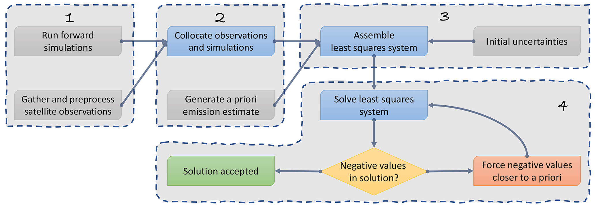
Figure 1 General solution framework for creating an accepted a posteriori emission estimate. The input to the algorithm is marked in gray (forward simulations, satellite observations, an a priori estimate, and initial uncertainties for both observations and a priori estimate). The algorithm runs sequentially through stages 1 to 4, marked as dashed boxes, and computes and iteratively refines the estimate in stage 4. The most computationally demanding stages are stage 1 (forward simulations), 2 (collocation of observations and simulations), and 3 (assembly of source–receptor matrix). Iteratively solving the least-squares system is highly efficient.

2 Mathematical formulation and solution framework

We base our inversion procedure on the approach taken by Seibert (2000) and adopted to ash emission by several authors (see, e.g., Stohl et al., 2011, and the references therein). Figure 1 shows the general solution framework which we use. We first compute a set of forward runs, representing possible emissions; collocate these with satellite observations; and finally assemble them into a source–receptor matrix. We then formulate the solution as a least-squares problem incorporating these collocated simulations and observations as well as an a priori estimate (initial guess) of the emission. Together with the uncertainties in the observations and an a priori estimate, we solve the least-squares problem to find the emission that recreates the observed satellite observations best (in a least-squares sense). As there is no guarantee of non-negative values in this process, we may end up with non-physical emissions. Negative emissions are forced closer to the (non-negative) a priori estimate by decreasing the uncertainty of these values and solving the least-squares problem again. This process is repeated until we have sufficiently few negative emissions. Other inversion methods (e.g., Pelley et al., 2021) use an algorithm with a direct non-negative emission constraint.

2.1 Atmospheric dispersion model

For this work, we use the eEMEP (emergency European Monitoring and Evaluation Programme; Steensen et al., 2017b) model version rv4_17, which is the emergency version of the basic EMEP MSC-W chemical transport model (Simpson et al., 2012, 2018; EMEP MSC-W, 2018). The model is based on an Eulerian advection model, uses the fourth-order positive definite advection scheme of Bott (1989) and an ash particle diameter distribution with nine bins from 4 to 25 µm, and has gravitational settling in all model layers. It is used operationally to generate volcanic ash forecasts at the Norwegian Meteorological Institute, and these forecasts are published on the Avinor Internet Pilot Planning Centre web pages for all pilots to use.

The current operational setup uses 48 vertical hybrid sigma layers from the ground up to 9.26 hPa (around 26 km above sea level) with ECMWF meteorology. The layer thickness is smallest close to the ground and increases with altitude. For our use, this may not be the most efficient approach¹, and we instead use 22 vertical levels which are close to 650 m thick each, shown in Fig. 2. This is a trade-off between the number of levels to emit into (which corresponds to the system matrix size; see Sect. 2.2), and the computational time required to run the model. We restrict the vertical extent of our model to around 14 km due to limitations in the meteorological input fields available for the 2010 Eyjafjallajökull case.

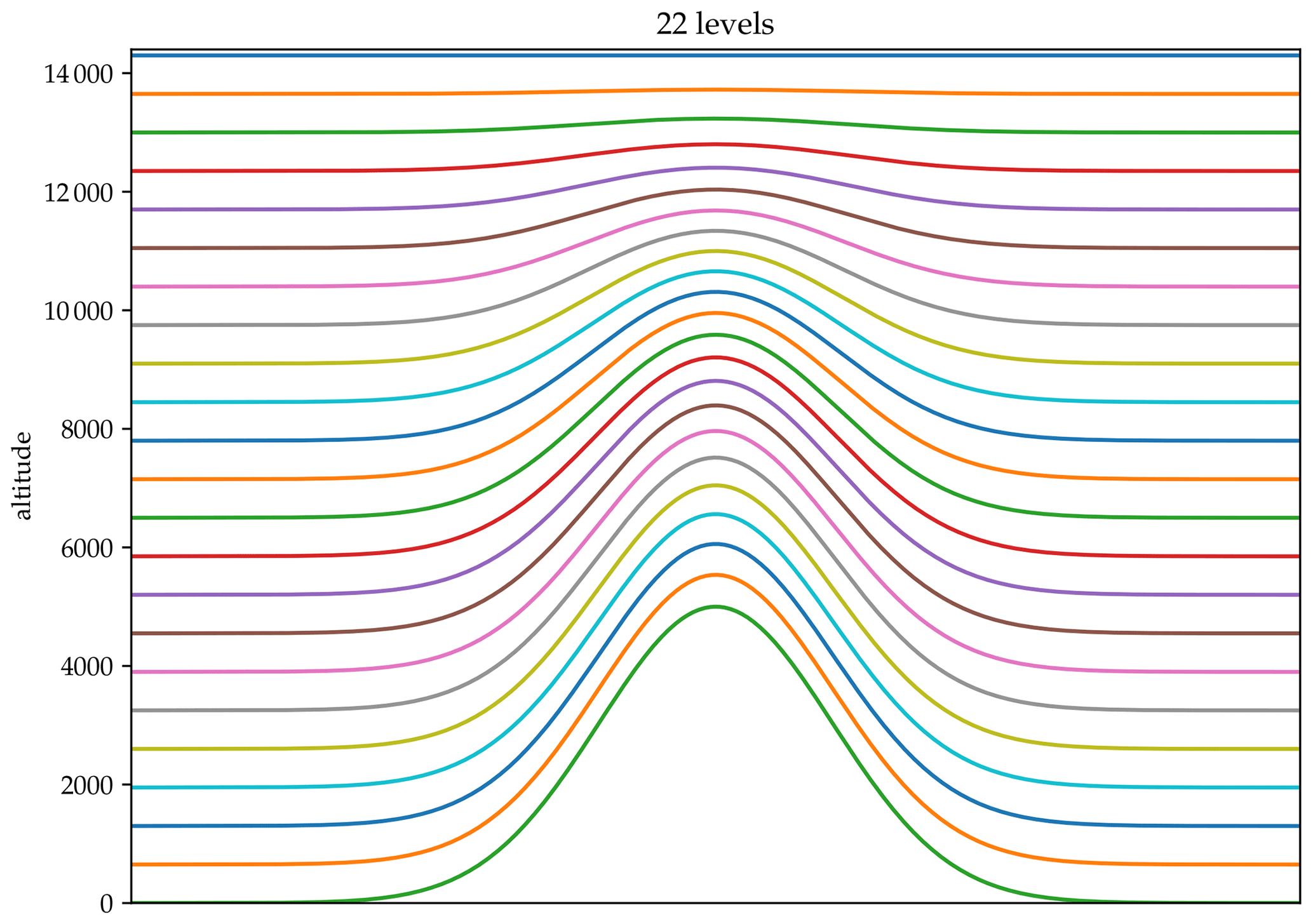
Figure 2 Vertical hybrid sigma levels for the inversion runs. Each level is designed to correspond to roughly 650 m of altitude given a ground pressure of 1013.25 hPa. The bottom layer shows a synthetic topography and how this alters the altitude of the different layers. Please note that these layers are only represented as hybrid sigma coordinates and never represent actual height as meters above sea level. The actual vertical-definitions file is available in Brodtkorb et al. (2020).

An inversion run with 22 levels of emission every 3 h for 4 d results in over 700 different unit emission scenarios that need to be simulated to generate the source–receptor matrix M. A regular run with the simulation model takes around 20 min to complete using 32 CPU cores, which means that this represents over 40 weeks of CPU time. This is prohibitively expensive, and we therefore use a special version of the eEMEP model that can run up to 19 tracers simultaneously. These tracers are independent and reduces the number of simulator runs from 700 to 36. The major savings come from only having to read and process the meteorology 36 times instead of over 700 times (which typically is the bottleneck for this kind of application).² The numerical advection and writing results to file are not optimized by this approach. For a simpler setup, we also do not use the uppermost three levels so that the 19 altitudes at each emission time can be simulated with a single run. We end up with 33 runs that each take around 20 min to complete, and using the Nebula supercomputer³ we are able to get all these inversion runs completed in less than 1 h.

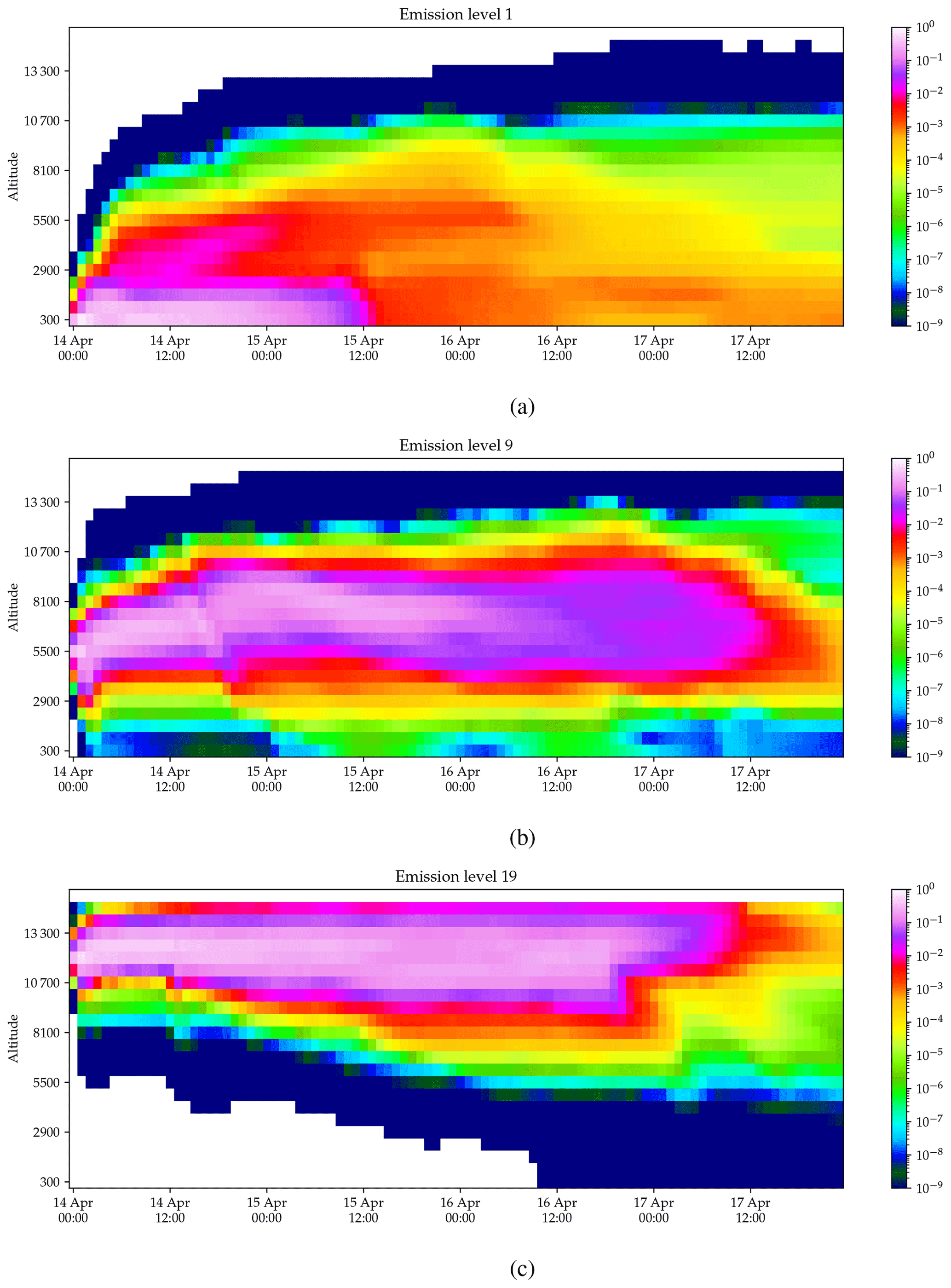
Figure 3 Unit emission profiles used in the inversion procedure. Here we emit a unit (1 Tg, teragram) of ash at different emission levels and plot the amount of ash in different layers over time. The figure has been created by spatially integrating the ash mass in each layer and thus shows how the ash emitted at a specific altitude disperses as time passes. The ash is released at the hybrid terrain-following vertical model levels shown in Fig. 2. Notice that for emissions close to ground, the ash travels only for a short time.

Figure 3 shows the result of emission simulations for different emission altitudes. The three simulations emit ash at level 1, 9, and 19 at midnight on 14 April. The simulation then progresses, and the plot shows how the ash is distributed in the vertical dimension as time goes on. Notice that large parts of the ash cloud leave the simulation domain⁴

2.2 Source–receptor matrix

The inversion procedure is based upon creating the so-called source–receptor matrix M from a set of forward simulations with unit emissions (see Fig. 3). We define the set of unit emissions as follows:

$$\begin{array}{}\text{(1)}& \begin{array}{rl}\mathit{\left\{}S\mathit{\right\}}& =\mathit{\left\{}S\right({\mathit{\alpha }}_{\mathrm{1}},{\mathit{\beta }}_{\mathrm{1}}),\mathrm{\dots },S({\mathit{\alpha }}_{\mathrm{1}},{\mathit{\beta }}_l),S({\mathit{\alpha }}_{\mathrm{2}},{\mathit{\beta }}_{\mathrm{1}}),\mathrm{\dots }S({\mathit{\alpha }}_k,{\mathit{\beta }}_l\left)\mathit{\right\}}\\ & =\mathit{\{}{S}_{\mathrm{1}},\mathrm{\dots },S_n\mathit{\}}.\end{array}\end{array}$$

Here, α_k denotes emission time k and β_l denotes emission level l. An individual simulation S_j then contains time-dependent three-dimensional simulation results of a unit of ash emitted into the atmosphere at the given emission time and emission level.

We equivalently have the set of observations arising from individual pixels of processed satellite images,

$$\begin{array}{}\text{(2)}& \begin{array}{rl}\mathit{\left\{}O\mathit{\right\}}& =\mathit{\left\{}O\right(y_{\mathrm{1}},x_{\mathrm{1}},t_{\mathrm{1}}),O(y_{\mathrm{2}},x_{\mathrm{2}},t_{\mathrm{2}}\left)\mathrm{\dots }O\right(y_m,x_m,t_m\left)\mathit{\right\}}\\ & =\mathit{\{}{O}_{\mathrm{1}},\mathrm{\dots },O_m\mathit{\}},\end{array}\end{array}$$

in which (x_i,y_i) denotes the spatial coordinates and (t_i) the observation time. The observations are sorted according to increasing time t_i. We can assemble matrix M so that element (i,j) of the matrix has simulation results from unit emission j at observation coordinate i,

$$\begin{array}{}\text{(3)}& {\mathbf{M}}_{i,j}:=S_j(y_i,x_i,t_i).\end{array}$$

We can similarly do this for the vector of observations so that element i corresponds to observation coordinate i,

$$\begin{array}{}\text{(4)}& {{\mathit{y}}_{\mathrm{0}}}_i:=O_i.\end{array}$$

This means that each row in the matrix corresponds to one observation and each column corresponds to a single simulated unit emission.

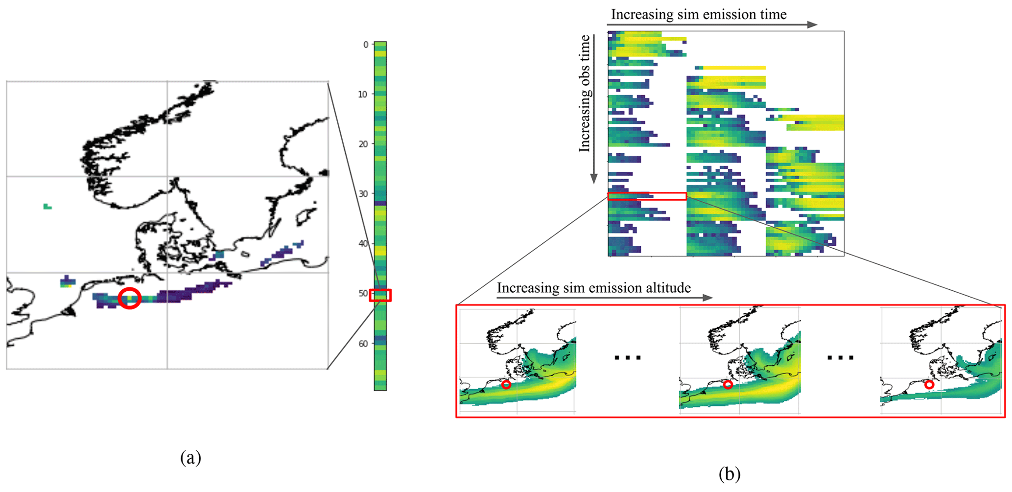
Figure 4 Linear system of equations. Panel (a) shows the vector of observations originating from the SEVIRI (Spinning Enhanced Visible and InfraRed Imager) instrument, in which a single location is highlighted with its corresponding location in the observation vector. Note that the image shows only part of the domain, and many of the detected ash pixels are outside the highlighted area. Panel (b) shows the source–receptor matrix M. Each row in the matrix contains all simulated ash mass loadings at the observation coordinate of the observation in the same row in the observation vector (see also Eq. 3). Equivalently, each column in the matrix corresponds to one individual emission simulation S_j. The matrix shown here has 60 observations (columns), 3 emission time points, and 19 emission altitudes (3×19 rows). White means no ash in the simulation, and the colored elements correspond to the concentration of ash in the individual simulations. See also Fig. 5, which shows the full matrix.

Figure 4 shows a small source–receptor matrix and part of the inputs used to create it. For each observation at $(y_i,x_i,t_i)$, we find the simulated ash content at the same time and spatial coordinate for all of the different emission simulations.

With the source–receptor matrix assembled, the aim of the inversion procedure is to find vector x so that

$$\begin{array}{}\text{(5)}& \mathbf{M}\mathit{x}={\mathit{y}}_{\mathrm{0}}.\end{array}$$

Here, x is the linear combination of unit emissions that best reproduce the observations. In an ideal world, we could have hope of finding the vector of unit emissions x that reproduces our observations. However, in the presence of observation and simulation uncertainties, we instead have to resort to finding the vector that best represents our observations.

The size of the matrices and vectors involved in the computation is determined by the number of observations and unit emissions. The number of unit emissions n can typically be a few hundred to a few thousand, and the number of observations m can be hundreds of thousands or even millions. For example, for the beginning of the 2010 Eyjafjallajökull eruption (to be discussed later in Sect. 4), we have an emission simulation every 3 h starting at 00:00 UTC on 14 April an continuing to 00:00 UTC on 18 April and emission heights every 650 m up to about 12 km. This corresponds to 33 distinct times and 19 elevations, totaling to 627 unique unit emissions with one simulation each. The corresponding satellite images for this period has a total of 92 403 observations, leading to an overdetermined system (i.e., 92 403 constraints and 627 degrees of freedom).

2.3 Linear least squares with Tikhonov regularization

We cannot hope to solve the system in Eq. (5) exactly, as it is typically overdetermined and both the simulations and observations have errors. We therefore seek a solution for vector x using linear least squares with Tikhonov regularization. The aim is to find a smooth solution that accounts for both observational and modeling errors.

Using (ground/visual) observations of the eruption, we create an a priori estimate of emission x_a and incorporate this a priori knowledge into our least-squares solver to give preference to solutions close to the a priori estimate. We start by replacing our inverted emissions x with $\stackrel{\mathrm{̃}}{\mathit{x}}=\mathit{x}-{\mathit{x}}_{\mathrm{a}}$,

$$\begin{array}{ll}{\displaystyle }\mathbf{M}\mathit{x}& {\displaystyle }={\mathit{y}}_{\mathrm{0}},\\ {\displaystyle }\mathbf{M}(\mathit{x}-{\mathit{x}}_{\mathrm{a}})& {\displaystyle }={\mathit{y}}_{\mathrm{0}}-\mathbf{M}{\mathit{x}}_{\mathrm{a}},\\ {\displaystyle }\mathbf{M}\stackrel{\mathrm{̃}}{\mathit{x}}& {\displaystyle }=\stackrel{\mathrm{̃}}{\mathit{y}},\end{array}$$

to penalize solutions that lie far from our a priori estimate. We still cannot hope to find an exact solution to this problem, but we can find the optimal solution, in a least-squares sense, by minimization:

$$J_{\mathrm{1}}=\left|\right|\mathbf{M}\stackrel{\mathrm{̃}}{\mathit{x}}-\stackrel{\mathrm{̃}}{\mathit{y}}\left|\right|.$$

However, the observations are known to have measurement error, and this uncertainty can be included by assigning a weight to each observation:

$$\begin{array}{}\text{(6)}& J_{\mathrm{1}}=\left|\right|{\mathit{\sigma }}_{\mathrm{o}}^{-\mathrm{1}}\left(\mathbf{M}\stackrel{\mathrm{̃}}{\mathit{x}}-\stackrel{\mathrm{̃}}{\mathit{y}}\right)\left|\right|,\end{array}$$

in which σ_o is a diagonal matrix with the standard error of observations to control how close we want our computed solution to match observation ${{\mathit{y}}_{\mathrm{0}}}_i$.

In the formulation above, we can also control how closely we want our solution to lie to the observations. To control how closely our solution should lie to the a priori knowledge, we add a second minimization term,

$$\begin{array}{}\text{(7)}& J_{\mathrm{2}}=\left|\right|{\mathit{\sigma }}_x^{-\mathrm{1}}(\mathit{x}-{\mathit{x}}_{\mathrm{a}})\left|\right|=\left|\right|{\mathit{\sigma }}_x^{-\mathrm{1}}\stackrel{\mathrm{̃}}{\mathit{x}}\left|\right|,\end{array}$$

where σ_x is a matrix with the estimated standard error of the a priori estimates on the diagonal. In our experiments, we have used ${\mathit{\sigma }}_x=\frac{\mathrm{1}}{\mathrm{2}}{\mathit{x}}_{\mathrm{a}}$.

Unfortunately, solving this minimization problem often results in implausible solutions with non-physical discontinuities in the vertical dimension. To avoid such non-physical solutions, we can add a smoothness minimization term,

$$\begin{array}{}\text{(8)}& J_{\mathrm{3}}=\mathit{ϵ}\left|\right|\mathbf{D}\stackrel{\mathrm{̃}}{\mathit{x}}\left|\right|,\end{array}$$

in which D is a tridiagonal matrix that calculates the second derivative of $\stackrel{\mathrm{̃}}{\mathit{x}}$, and ϵ determines how smooth we want the solution to be. We have used $\mathit{ϵ}=\mathrm{1.0}{e}^{-\mathrm{3}}$, and this parameter is typically set by experimentation.

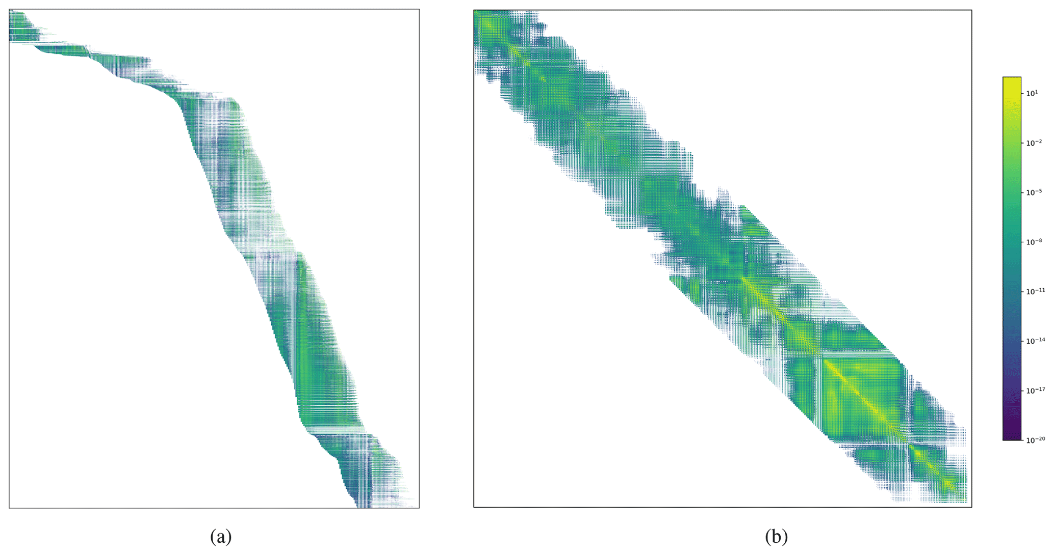
Figure 5 (a) Source–receptor matrix M and (b) least-squares matrix G. The source–receptor matrix for the Eyjafjallajökull case without no-ash observations for the period 14 April–24 May has 736 494 rows (observations) and 6061 columns (ash emissions to estimate). It has approximately 521 million non-zero entries. The least-squares matrix is a square matrix with 6061 rows and columns. The band width of the matrix is approximately 2000, which is determined by the maximum allowable time between an emission and observation of ash.

We can solve these combined minimization problems as a Tikhonov regularization problem (with a Tikhonov matrix of $\mathbf{Q}={\mathit{\sigma }}_x^{-\mathrm{2}}+\mathit{ϵ}{\mathbf{D}}^T\mathbf{D}$),

$$[{\mathbf{M}}^T{\mathit{\sigma }}_{\mathrm{o}}^{-\mathrm{2}}\mathbf{M}+{\mathit{\sigma }}_x^{-\mathrm{2}}+\mathit{ϵ}{\mathbf{D}}^T\mathbf{D}]\stackrel{\mathrm{̃}}{\mathit{x}}={\mathbf{M}}^T{\mathit{\sigma }}_{\mathrm{o}}^{-\mathrm{2}}\stackrel{\mathrm{̃}}{\mathit{y}},$$

in which the optimal solution x can be computed as

$$\begin{array}{}\text{(9)}& \begin{array}{rl}\mathit{x}& ={\mathit{x}}_{\mathrm{a}}+[{\mathbf{M}}^T{\mathit{\sigma }}_{\mathrm{o}}^{-\mathrm{2}}\mathbf{M}+{\mathit{\sigma }}_x^{-\mathrm{2}}+\mathit{ϵ}{\mathbf{D}}^T\mathbf{D}{]}^{-\mathrm{1}}{\mathbf{M}}^T{\mathit{\sigma }}_{\mathrm{o}}^{-\mathrm{2}}\stackrel{\mathrm{̃}}{\mathit{y}}\\ & ={\mathit{x}}_{\mathrm{a}}+{\mathbf{G}}^{-\mathrm{1}}{\mathbf{M}}^T{\mathit{\sigma }}_{\mathrm{o}}^{-\mathrm{2}}\stackrel{\mathrm{̃}}{\mathit{y}}\\ & ={\mathit{x}}_{\mathrm{a}}+{\mathbf{G}}^{-\mathrm{1}}\mathit{B}.\end{array}\end{array}$$

Figure 5 shows both the source–receptor matrix M and the least-squares matrix G, which then is used to compute the a posteriori emission estimates x. M is generally a large sparse matrix with m rows (one per observation O_i) and n columns (one per emission S_j), whilst G is a relatively small banded matrix with n rows and columns. The band width depends on the maximum time from emission to observation and is 1824 for our typical inversion parameters (19 emissions eight times per day for 6 d).

It is important that the units of the matrices and vectors are compatible when formulating the minimization problem. Our source–receptor matrix M and observation vector y₀ are column loadings expressed in kg m⁻². The a priori emission estimate x_a is mass-scaled to teragrams (10¹² g), and our individual simulations S_j have a source term from the volcano that emits one teragram of ash at the given time point α and altitude β. This means that our computed solution x is given in teragrams of emitted ash.

2.4 Efficient computation of a least-squares matrix

One novelty in this paper is the efficient assembly and calculation of the least-squares matrix, enabling the inversion to run on a regular laptop computer. The linear system in Eq. (5) is solved using the Tikhonov regularization, formulated as

$$\begin{array}{}\text{(10)}& {\displaystyle }\mathit{x}={\mathit{x}}_{\mathrm{a}}+{\mathbf{G}}^{-\mathrm{1}}\mathit{B}\end{array}$$

by inverting the least-squares matrix G. G is a matrix of dimension n×n, in which n is the number of emissions we want to estimate. This matrix is computed from the larger matrix M of size m×n, in which m is the number of observations. For the full Eyjafjallajökull eruption case, that means that up to 56 536 603 observations⁵ are used to calculate the 6061 unknown emissions.

The 56.5 million observations are matched against the simulations and stored in matrix M so that each row has up to 912 non-zero entries (19 emissions eight times per day for 6 d) but an average of around 170 in our runs. The matrix then has approximately 9.7 billion non-zeroes, which corresponds to 72.27 GiB of data. This is prohibitively expensive for the inversion procedure and limits the number of observations that are possible to assimilate. However, by carefully examining and restructuring the products involved, we can reformulate the procedure to compute G directly without storing M. This reduces the memory requirement from the aforementioned 72 GiB to less than 300 MB (a improvement of a factor of 260), enabling efficient inversion even on laptop computers with no special hardware requirements.

Matrix G in Eq. (9) is computed using

$$\begin{array}{}\text{(11)}& {\displaystyle }\mathbf{G}{\displaystyle }={\mathbf{M}}^T{\mathit{\sigma }}_{\mathrm{o}}^{-\mathrm{2}}\mathbf{M}+{\mathit{\sigma }}_x^{-\mathrm{2}}+\mathit{ϵ}{\mathbf{D}}^T\mathbf{D}.\end{array}$$

Here, M is the enormous sparse matrix with 72 GiB of non-zero entries, whilst G is a relatively modest dense matrix. The classical way to compute this expression is to use the inner product,

$$\begin{array}{}\text{(12)}& \begin{array}{rl}{\left({\mathbf{M}}^T{\mathit{\sigma }}_{\mathrm{o}}^{-\mathrm{2}}\mathbf{M}\right)}_{i,j}& =\text{diag}\left({\mathit{\sigma }}_{\mathrm{o}}^{-\mathrm{2}}\right)\circ ({\mathbf{M}}_{:,i}\cdot {\mathbf{M}}_{:,j})\\ & =\sum _{k=\mathrm{1}}^m{{\mathit{\sigma }}_{\mathrm{o}}}_k^{-\mathrm{2}}{\mathbf{M}}_{k,i}\cdot {\mathbf{M}}_{k,j}\\ & ={{\mathit{\sigma }}_{\mathrm{o}}}_{\mathrm{1}}^{-\mathrm{2}}{\mathbf{M}}_{\mathrm{1},i}\cdot {\mathbf{M}}_{\mathrm{1},j}+\mathrm{\dots }\\ & +{{\mathit{\sigma }}_{\mathrm{o}}}_m^{-\mathrm{2}}{\mathbf{M}}_{m,i}\cdot {\mathbf{M}}_{m,j},\end{array}\end{array}$$

in which $\text{diag}\left({\mathit{\sigma }}_{\mathrm{o}}^{-\mathrm{2}}\right)$ is the vector composed of the diagonal entries of ${\mathit{\sigma }}_{\mathrm{o}}^{-\mathrm{2}}$. Recall that m is here the number of observations.

By examining this inner product, we see that we can compute matrix G as a sum of outer products for each row of M instead of the inner-product formulation for each column above:

$$\begin{array}{}\text{(13)}& \mathbf{G}=\sum _{k=\mathrm{1}}^m{{\mathit{\sigma }}_{\mathrm{o}}}_k^{-\mathrm{2}}{\mathbf{M}}_{k,:}\otimes {\mathbf{M}}_{k,:}+{\mathit{\sigma }}_x^{-\mathrm{2}}+\mathit{ϵ}{\mathbf{D}}^T\mathbf{D}.\end{array}$$

By using the outer product, we can avoid having to store the large matrix M in memory and instead store only the relatively small n×n matrix. For the full Eyjafjallajökull eruption case that means that we store a dense matrix of 6061×6061 elements, which takes less than 300 MB of memory. In essence, this means that we assemble matrix G using one observation at a time.

Unfortunately, this also means that we need to compute

$$\begin{array}{}\text{(14)}& \mathit{B}={\mathbf{M}}^T{\mathit{\sigma }}_{\mathrm{o}}^{-\mathrm{2}}\stackrel{\mathrm{̃}}{\mathit{y}}={\mathbf{M}}^T{\mathit{\sigma }}_{\mathrm{o}}^{-\mathrm{2}}({\mathit{y}}_{\mathrm{0}}-\mathbf{M}{\mathit{x}}_{\mathrm{a}})\end{array}$$

simultaneously. Whilst this does not seem to have a significant impact, it means that we can no longer change our a priori estimate x_a without also re-assembling the right-hand side. However, it is trivial to use matrix X_a, in which each column represents one a priori estimate, and solve for all these simultaneously.

Equations (12) and (13) represent two extremes in how to compute matrix G, in which the former first assembles M and computes G using the (sparse) matrix product and the latter assembles G directly one observation at a time using the outer product. We can also use a hybrid approach in which we assemble a set of observations into G simultaneously. If we create a row partition of M and call each partition ${\mathbf{Q}}_{<\mathrm{1}>},\mathrm{\dots },{\mathbf{Q}}_{<p>}$, we can compute the same product as follows:

$$\begin{array}{}\text{(15)}& \mathbf{G}=\sum _{k=\mathrm{1}}^p{\mathbf{Q}}_{<k>}^T{\mathit{\sigma }}_{\mathrm{o}}^{-\mathrm{2}}{\mathbf{Q}}_{<k>}+{\mathit{\sigma }}_x^{-\mathrm{2}}+\mathit{ϵ}{\mathbf{D}}^T\mathbf{D}.\end{array}$$

This is analogous to computing Eq. (12) for a subset of the rows of M at a time or a subset of observations at a time. The benefit of this hybrid approach is that the computational speed can increase dramatically, as we can use efficient dense linear algebra routines from Python libraries, thereby avoiding the prohibitive memory requirement of Eq. (12) as well as the expensive outer-product formulation required for Eq. (13). The total performance benefit of the hybrid approach is up to 15 times in terms of wall clock time spent assembling and computing the least-squares matrix.

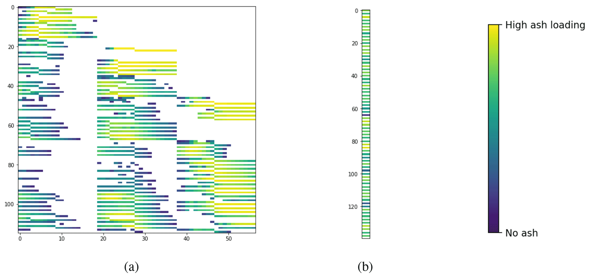
Figure 6 Linear system of equations with altitude information. Panel (a) shows the source–receptor matrix M with altitude information, and panel (b) is the corresponding vector of observations. Compare with Fig. 4 and notice that each row is now split into two new rows. Even-numbered rows now correspond to observations of ash (below the detected ash plume height), and odd-numbered rows correspond to no ash. The rest of the solution procedure remains the same.

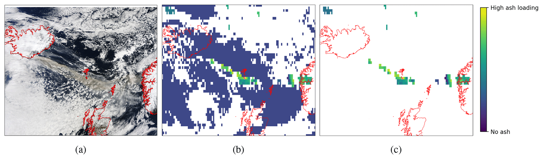
Figure 7 Satellite image and corresponding detection of ash. Panel (a) is from NASA Terra MODIS 2010/105 on 15 April 2010 at 11:35 UTC, and panel (b) is from the SEVIRI satellite instrument after the detection of ash concentrations at 11:00 UTC. White pixels are unobserved or uncertain parts of the domain, and blue pixels are observations of no ash. Panel (c) shows only certain instances of non-zero detection of ash.

2.5 Iterative inversion procedure

Because there are large uncertainties in both the meteorology and the satellite observations (see, e.g., Harvey et al., 2022), we may end up with negative emission estimates at certain points, as there is nothing in our minimization problem that prohibits negative solutions. Negative values in the a posteriori data are forced to lie closer to the a priori estimate by reducing the uncertainties σ_x for these values and recomputing the solution. The iterative procedure repeats until the amount of negative ash emissions is reduced to a fraction (e.g., 1 %) of the total a posteriori emission estimate.

2.6 Including ash cloud-top information

A novelty in this paper is the use of observed altitude from, e.g., the SLSTR instrument. The dual-view capabilities of the SLSTR instrument may be used to detect the top of the ash plume and thereby restrict the inversion procedure to give more correct altitudes for the a posteriori emissions. Mathematically, we formulate this by splitting each observation into two observations: one non-zero observation from the ground up to the detected plume height and one zero observation from the plume height to the top of the model. In essence, we simply split each row in the source–receptor matrix M into two as shown in Fig. 6. This then doubles the number of rows in the matrix, whilst keeping the number of non-zeroes constant. The rest of the algorithm is unchanged.

The computational cost of this extra information is negligible for the whole algorithm as our final linear least-squares system G has the same dimension both with and without altitude information.

3 Verification using synthetic data

To check if the inversion procedure presented here works as intended is a non-trivial exercise, as there are large uncertainties in both the simulation model and observations being used. We have therefore checked our inversion procedure against a known truth, generated by the simulation model itself. We first generate an a priori emission estimate using radar observed plume heights and the mass eruption rate estimate in Mastin et al. (2009) and subsequently use this a priori estimate to generate synthetic satellite images. The synthetic satellite images are created by scaling the unit emission simulations with the a priori value and then vertically integrating them to yield grams per square meters. We observe these satellite images at random locations in space and time to generate the truth. We then expect that our inversion procedure should generate a posteriori data which lie close to the a priori estimate used to generate the truth. It should be noted that we do not expect a perfect inversion, as we try to estimate the vertical and time distribution of the ash emission, whilst we only observe the vertically integrated ash concentration at certain points. We have used the 2010 Eyjafjallajökull eruption as a basis to generate a realistic scenario from 14 to 18 April. We also vary the a priori estimate and the ash cloud-top altitude to see the effect of these parameters on the solution. It should also be noted that synthetic benchmarks remove any uncertainty in both the transport model and the numerical weather forecast data.

We have devised several different experiments to test the inversion, which are summarized in Table 1. The expected outcomes of the experiments are as follows:

• A.

  This case uses an a priori estimate that is identical to the truth, and the inversion procedure should be able to produce something close to the truth. These default a priori data are created using an estimate of the eruption altitude and the relationship given by Mastin et al. (2009). Because we are using a Tikhonov regularization, we will expect a small deviation between the default a priori data and the computed a posteriori data. If the inversion is unable to capture this state, we expect that something is wrong – either with the implementation or with the data.

• B.

  This case uses the default a priori data, but the truth has an emission altitude of half the a priori data. As the inversion does not use altitude information in the inversion, we may not be able to resolve this case.

• C.

  This case is identical to case B, but we use the altitude information in the inversion. Case B and C therefore showcase the added value of restricting the inversion with altitude information in the case we have a too large an altitude estimate for the a priori data.

• D.

  This case shows how the inversion handles a constant a priori estimate without the use of altitudes in the inversion procedure. This is to simulate a “worst-case scenario” in which we do not have a good description of the eruption and therefore only have a very crude a priori estimate.

• E.

  This case is identical to case D but now using altitude information in the inversion.

All of these cases use synthetically generated satellite observations (shown in Fig. 8) in the inversion. These synthetic satellite observations are generated by first multiplying the true a posteriori data with the simulated emissions, followed by vertically integrating to achieve a column load for the whole domain. We finally sample at random locations to simulate true satellite images. The synthetic dataset consists of 235 observation time points with a total of 462 654 ash observations and covers the domain shown in Fig. 8.

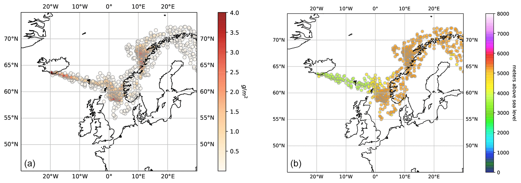
Figure 8 Synthetic satellite observations used in the validation of the inversion procedure with (a) mass loading (g m²) and (b) ash cloud-top altitude (m). The synthetic observations are based upon a vertical integration of simulation results at specific coordinates. The figure shows a synthetic satellite observation from 10:00 UTC on 15 April using the standard a priori estimate shown in Fig. 9 (compare also with Fig. 7, which shows actual satellite data). The coordinates are randomly generated and consist of 774 observation points uniformly distributed in space.

Table 1 Summary of experiments using synthetic data. The observations column shows what kind of synthetic observations are being used. The observations are generated using an eruption using the default a priori emission (“default”) or using the same amount of emission as the default a priori data but with half the plume height (“half altitude”). The a priori estimate used is either the default or a constant estimate based on an 8.4 km plume height.

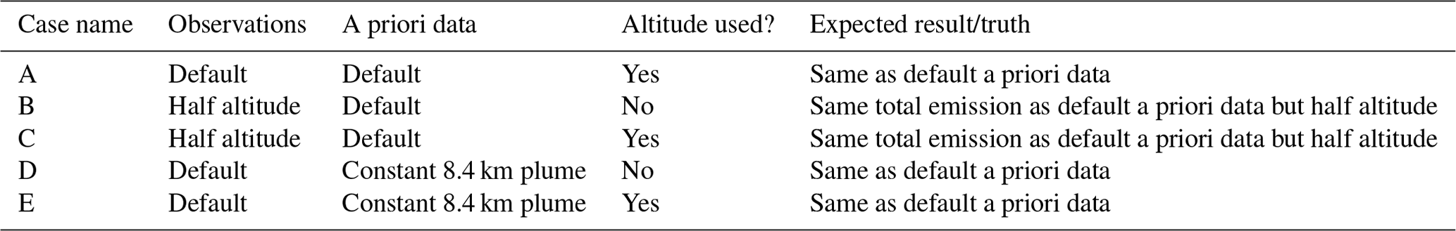
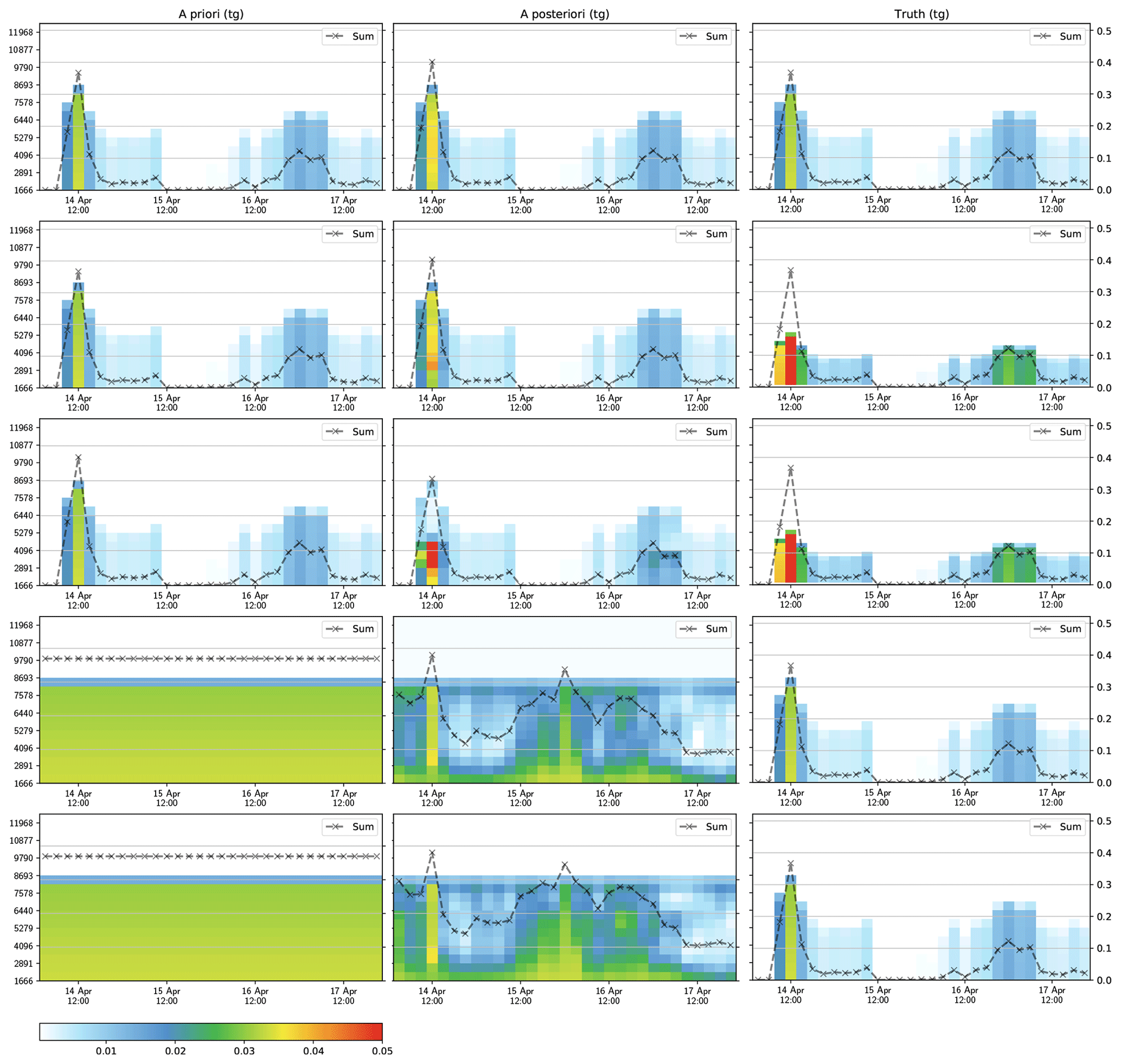
Figure 9 Verification of the inversion code. The color bar is in teragrams of emitted fine ash, and the altitude is in meters above sea level (volcano altitude is 1666 m above sea level). The rows (from top) represent the five cases (A–E) outlined in Table 1. The left column shows the a priori data used in the inversion, the middle column shows the inverted a posteriori estimate, and the right column shows the truth. The left axis shows the emission altitude above sea level, and the right axis shows the total emission in teragrams. The first row uses a priori data equal to the truth (case A), the second and third rows use a truth in which the ash is emitted at half the altitude of the a priori data (cases B and C), and the fourth and fifth rows use a constant a priori estimate (cases D and E). The first (case A), third (case C), and fifth rows (case E) use ash cloud-top observations to restrict the inversion.

Figure 9 shows the result of running the verification experiments. For case A (the top row) the inversion algorithm is quite capable of recovering the truth. The inverted results show a slight increase in the total emission, in particular during the peak of the eruption on 14 April. However, the inverted results are overall in good agreement with the expected results.

For case B, shown in the second row, the effect of overestimating the altitude of the eruption in the a priori estimate is evident, illustrating that the inversion does not capture the true emission very well. However, the result is not very surprising as the inversion algorithm is only using observations of vertically integrated quantities. Without a restriction on the altitude in the inversion itself, there needs to be a significant difference in the prevailing winds at different altitudes to penalize emissions at wrong altitudes.

Case C in the third row shows the exact same experiment as in the second row, but this time we use observations of the ash cloud top to restrict the inversion. Compared with case B, we clearly see the benefit of using altitude observations. The inversion is capable of capturing the emission altitude very well during the peak of the eruption on 14 April and also shows a relatively good reduction in higher-altitude emissions during the eruption from 16 to 17 April.

Case D and E are shown in the final two rows, which show how the inversion algorithm behaves when we do not have a good a priori estimate of the eruption. The results show that both with and without altitude observations, the algorithm is unable to find a satisfactory result. The two experiments are able to capture the peak of the eruption on 14 April quite well but wrongfully estimate a larger eruption from 15 to 16 April. This can be explained by our synthetic satellite observations shown in Fig. 8, which do not include observations of no ash. Thus, the algorithm does not have sufficient observations to restrict the inversion, particularly the eruption-free period from 15 to 16 April.

4 Validation using the 2010 Eyjafjallajökull eruption

The previous section outlined some of the sensitivities of the inversion procedure on synthetic datasets, in which we have generated satellite observations from a synthetic known truth. In this section, we apply the methodology to a real-world eruption, the 2010 Eyjafjallajökull eruption. The Eyjafjallajökull eruption is a well-studied case which makes it possible to compare the quality of our results with other approaches.

We have run two scenarios with our inversion code. The first uses the same setup as Steensen et al. (2017a) and covers the onset of the eruption from 14 to 18 April with an a priori estimate from eruption altitude and the relationship given by Mastin et al. (2009). The second mimics the setup of Stohl et al. (2011) and covers the whole eruption from 14 April to 24 May with a more complex a priori estimate. The full dataset consists of 959 observation time points and a total of 876 906 non-zero observations (detected ash), and the eruption onset dataset is simply a subset of the 96 first observation time points with a total of 43 241 non-zero observations. The extent of the dataset is shown in Fig. 11.

4.1 Eyjafjallajökull eruption onset

In this case, we use the same setup as in Steensen et al. (2017a) and have, as far as possible, used the same parameters. We have used the same SEVIRI satellite data and simulated unit emission simulations with the eEMEP advection model.

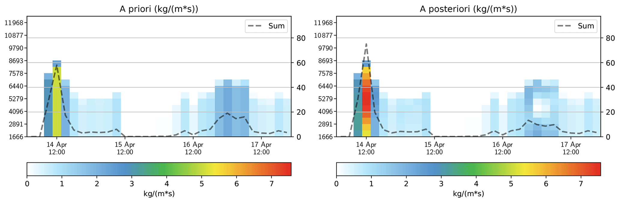
Figure 10 Comparison of the a priori estimate with the inverted results (kg (m s)⁻¹) for the Eyjafjallajökull eruption onset. The altitude is in meters above sea level (volcano altitude is 1666 m above sea level). The dashed line shows the total erupted mass in teragrams.

Figure 10 shows the result of the inversion algorithm. Overall our results match those of Steensen et al. (2017a), but there are some differences. We find that the main emissions for 14 April are fairly evenly spread from 3 to 7 km, with a maximum around 5 km, while in Steensen et al. (2017a) the emissions peak around 8 km and there is no emission below 3 km; secondly, early on 17 April we find emissions below 6 km, while none are reported by Steensen et al. (2017a). It is noted that results presented here agree better with those presented by (Fig. 2c of Stohl et al., 2011). We have identified several possible reasons for the differences with Steensen et al. (2017a): this is a new implementation, and we have used different parameters in the simulation runs with eEMEP; there are different parameters used in the inversion run; there is a slightly different vertical discretization of the eEMEP model; and the advection model (eEMEP) has gone through significant upgrades and changes. As the details required to reproduce the runs of Steensen et al. (2017a) are not fully available, it is not possible to reproduce their results.

4.2 Eyjafjallajökull full eruption

We use a similar setup as in Stohl et al. (2011) in the inversion of the full eruption period of Eyjafjallajökull, lasting from 14 April to around 24 May 2010. Our inversion results (Fig. 12) show a clear reduction in the eruption strength around 16 April, as well as the two high-altitude eruptions on 14 and 16 May, and a significant increase in the eruption strength on 12–13 May. Our results generally match well with those of Stohl et al. (2011), but there are some differences. In particular, the eruption onset on 14 April appears to be stronger in our results, and our results maintain more ash in the a posteriori data below 3 km. There are several factors that contribute to these differences: different advection models are used (eEMEP and FLEXPART, FLEXible PARTicle dispersion model); different meteorological datasets (ECMWF and a combination of ECMWF and GFS, Global Forecast System); differences in analysis of satellite observations; and a similar but not identical a priori estimate.

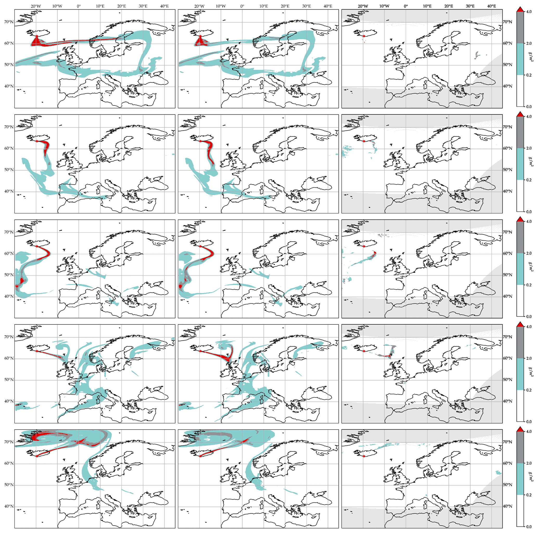
Figure 11 Modeled and observed ash clouds over Europe during the 2010 Eyjafjallajökull eruption at different times. From top to bottom, the figures represent 17 April 2010 at 19:00 UTC, 6 May 2010 at 10:00 UTC, 8 May 2010 at 19:00 UTC, 13 May 2010 at 03:00 UTC, and 18 May 2010 at 16:00 UTC. The leftmost column shows the modeled a priori estimate, the next column shows the modeled a posteriori estimate after inversion, and the rightmost column shows the satellite image. The colors in the figures correspond to the color codes used operationally at the Internet Pilot Planning Centre (IPPC) operated by Avinor Air Navigation Services AS (https://ippc.no/, last access: 21 February 2024). The color codes groups total column loadings into no ash (<0.2 g m⁻²), low ash (0.2–2.0 g m⁻²), medium ash (2.0–4.0 g m⁻²), and high ash (>4.0 g m⁻²). For the satellite images, non-analyzed areas are in light gray.

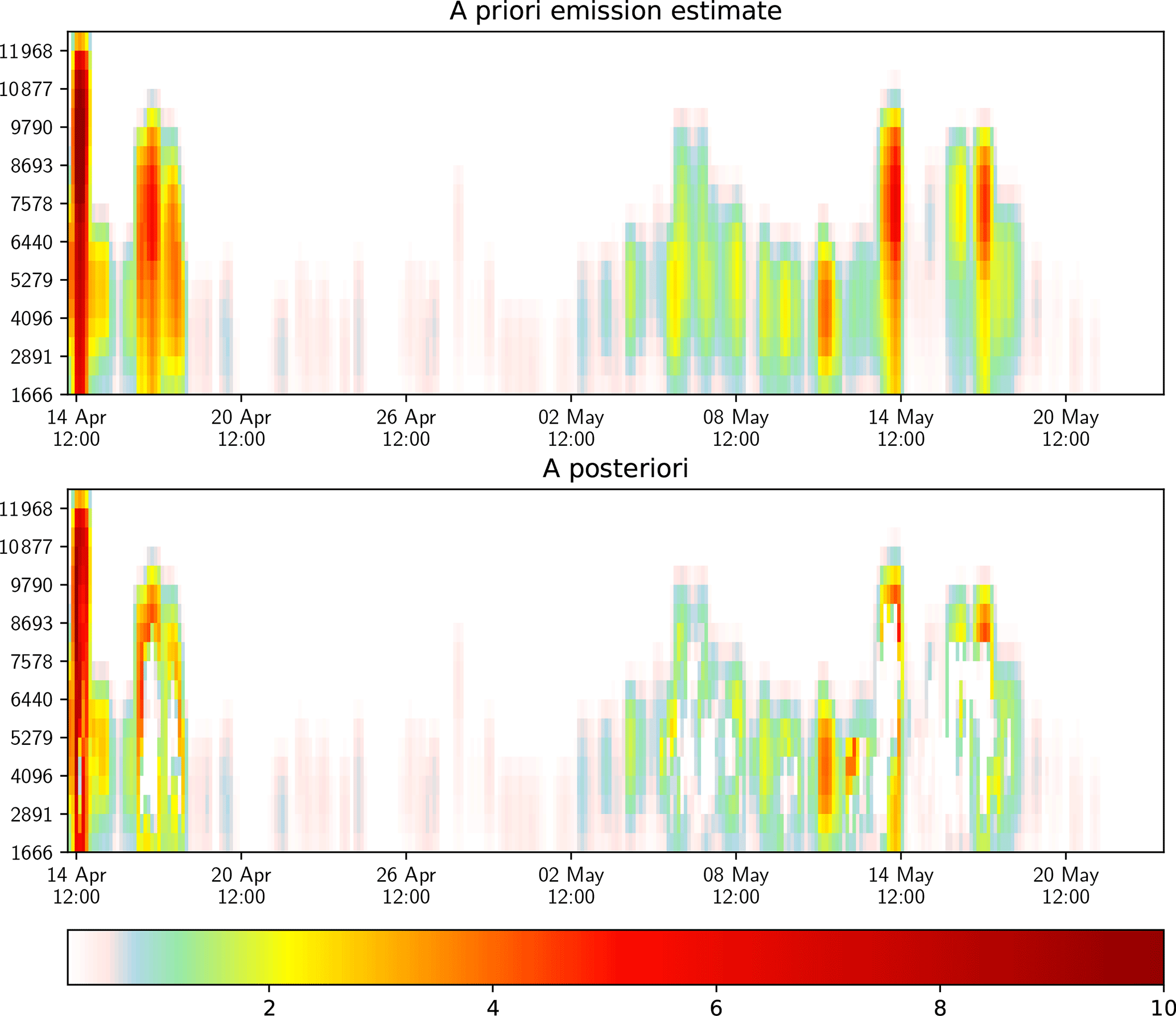
Figure 12 Eyjafjallajökull full eruption a priori vs. inverted emission estimate (kg (m s)⁻¹). The altitude is in meters above sea level, and the volcano summit is at 1666 m above sea level.

Figure 11 compares our a priori and a posteriori results with the retrieved ash from satellite observations for five different time points during the eruption. The figure shows quantized results in the same color scheme as the official Norwegian volcanic ash reports used by airline pilots⁶, with total column loadings of no ash (<0.2 g m⁻²), low ash (0.2–2.0 g m⁻²), medium ash (2.0–4.0 g m⁻²), and high ash (>4.0 g m⁻²). The left column shows the a priori estimate, the central column shows the a posteriori result, and the right column shows the satellite images.

The satellite images illustrate that the observations of ash are relatively sparse and that they suffer from false positives (including detected ash far from the simulated ash cloud; see also Fig. 7). They also show that there are differences between the position of the modeled and observed ash clouds, as shown in the fourth row close to the Faroe Islands. This is possibly due to errors in meteorology driving the advection model. Both false positives and positional errors between observed and modeled ash clouds make the inversion scenario significantly more challenging than the idealized data used for the verification in Sect. 3.

If we compare the a priori estimate with the a posteriori results, we see that the inversion algorithm reduces the areas with high-ash column loadings during parts of the eruption (first, third and fifth rows), whilst increasing it at other time points (second and fourth rows). Overall, this matches well with the observations of ash in the satellite images.

5 Performance assessment

The inversion framework consists of the four main stages (Fig. 1), and we have optimized each of these. The most novel improvements and optimizations have been in the assembly of the least-squares system in stage 3, but the other stages have also been improved.

In stage 1, we simulate the time development of unit emissions for a given altitude and time. This requires over 6000 unique simulation results, which is reduced to 319 eEMEP runs by using tracers (see also Sect. 2.1). Still, each run can take up to 40 min to complete, thus requiring over 200 computing hours on the Nebula supercomputer infrastructure. We have optimized the eEMEP runs by limiting the simulation time to a maximum of 6 d (thus assuming ash in the atmosphere older than 6 d will not be important for the inversion), which reduces the requirement to 110 computing hours on the cluster, as shown in Fig. 13. By running five simulations in parallel on the cluster, the wall clock time spent for the forward simulations is reduced to 10 h. By fully utilizing the cluster, it would be technically possible to reduce the wall clock time to approximately 1 h.

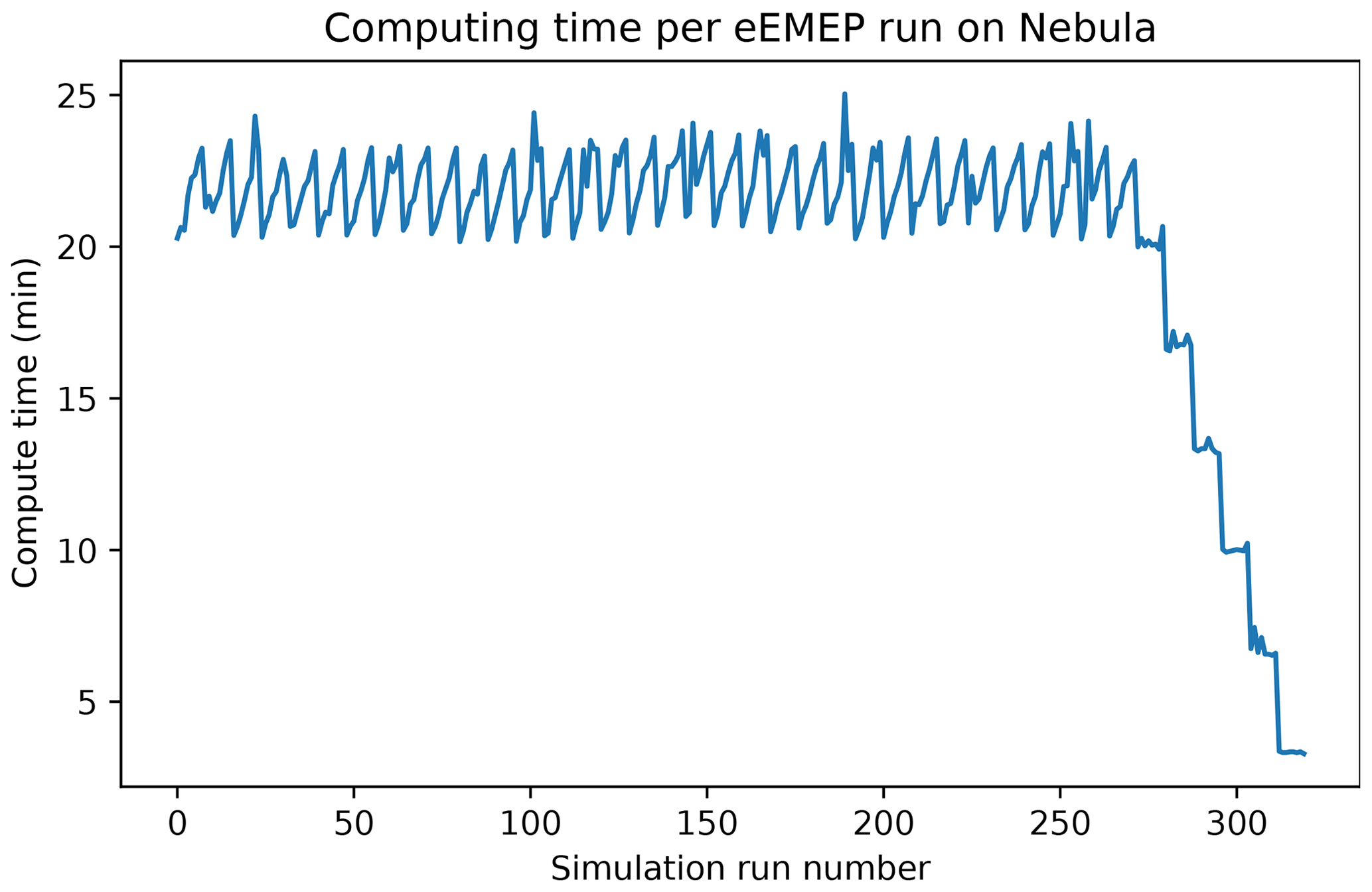
Figure 13 Computing time per forward simulation on the Nebula cluster. Notice that the last simulations take significantly less time as they approach the end simulation time (24 May 2010). The regular sawtooth pattern for the other runs is similarly explained by each new simulation starting at 00:00 UTC, even though the emission may start at, e.g., 21:00 UTC. This is due to a technical limitation in the eEMEP model.

Stage 2 is also a computationally demanding stage and consists of collocating all observations with the simulations created in stage 1 as well as generating the a priori estimate. The generation of the a priori estimate is not a computationally demanding challenge, but the collocation of observations is quite demanding as it requires us to match each observation to the unit emission simulation that might have caused it. This means that for each of the 56.5 million observations we have to find the corresponding temporospatial location in 912 unique simulations (see also Sect. 2.4). We can perform this on the PPI cluster⁷, and the process takes just shy of 5 h of wall clock time. This process is parallelizable (e.g., each of the 962 hourly satellite images can easily be processed independently), and it would be technically possible to significantly reduce the wall clock time by utilizing the full cluster.

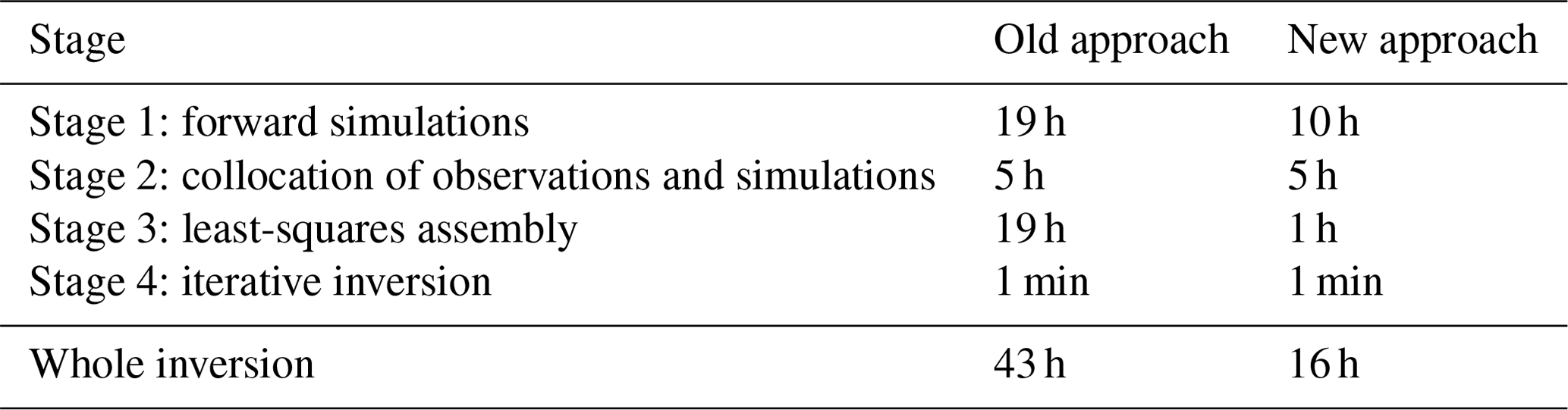
Table 2 Summary of wall clock time for the inversion procedure for the full Eyjafjallajökull eruption.

Finally, stage 3 is the last of the computationally demanding stages, in which we assemble the collocated simulations and observations into the least-squares system. This process takes over 19 h to complete on the PPI cluster when first assembling the huge matrix M and subsequently computing the matrix product ${\mathbf{M}}^T{\mathit{\sigma }}_{\mathrm{o}}^{-\mathrm{2}}\mathbf{M}$. The reformulation to compute matrix G directly reduces this process to just over 1 h. This stage may in fact also be parallelized further by following an approach similar to that shown in Eq. (15), i.e., partitioning the set of observations; assembling

$${\mathbf{G}}_q={\mathbf{Q}}_{<q>}^T{\mathit{\sigma }}_{\mathrm{o}}^{-\mathrm{2}}{\mathbf{Q}}_{<q>}+{\mathit{\sigma }}_x^{-\mathrm{2}}+\mathit{ϵ}{\mathbf{D}}^T\mathbf{D}$$

in parallel; and finally summing to compute the final matrix,

$$\mathbf{G}=\sum _{q=\mathrm{1}}^p{\mathbf{G}}_q.$$

The performance increases in this new approach are summarized in Table 2. In total, the inversion procedure runs approximately 2.7 times faster with the improvements discussed in this paper. Furthermore, an added benefit of the new inversion procedure is that it is extremely memory efficient, allowing it to run efficiently on a simple laptop.⁸

6 Summary and discussion

We have presented an inversion algorithm and open-source implementation for volcanic ash emission estimates based on satellite imagery. The main novelties of this paper include a memory-efficient algorithm for the assembly and calculation of the least-squares system, inclusion of ash cloud-top altitude information in the inversion, and verification using synthetic datasets. Our verification shows the potential benefit of using observations of the ash cloud top to restrict the inversion, and we have also run our code on the 2010 Eyjafjallajökull eruption. Our results are mostly in agreement with previously presented results but with some differences believed to be mainly due to differences in the model setup and meteorology used.

Our approach to assembling and calculating the least-squares system has reduced the computational time from over 19 h to just 1 h for this part of the inversion. For the simulation of the unit emissions, the computational time has gone from 19 to 10 h. These two stages constitute the most time-consuming parts of the inversion and reduce the total time to solution by a factor 2.7.

Our framework is also well tailored to an operational setting with an eruption going on for several weeks. It is technically possible to use a least-squares matrix G₁ representing, e.g., the first 3 d of the eruption and simply add another matrix G₂ that may represent a subsequent 4 d (and equivalently for vector B), instead of assembling the full 7 d period from scratch. With satellite imagery coming in continuously, this may save large amounts of computational time to create up-to-date estimates.

Our results show that using ash cloud-top altitude information gives a clear benefit, which contrasts the findings of Chai et al. (2017), who report a negative impact of using this information in the inversion. Our explanation to this is that we have performed testing with synthetic data in which there is no meteorological error. In the presence of meteorological error, we agree that there may be circumstances where adding more constraints to the inversion may negatively impact the results. Nevertheless, our results show that using ash cloud-top observations can improve the inversion results under favorable conditions.

This work has several opportunities for further improvement that we see natural to pursue. First of all, the use of coordinates in the collocation of satellite observations and simulations makes the inversion procedure sensitive to slight differences in the modeled vs. true meteorology. It would be fruitful to explore other forms of collocation strategies, e.g., using polar coordinates centered on the erupting volcano or at a streamlined distance from it, to possibly reduce this sensitivity. The use of ensemble meteorology coupled with ensemble inversion will possibly also address the sensitivity to differences between modeled and observed meteorology (see, e.g., Webster and Thomson, 2022; Crawford et al., 2022).

The current algorithm is somewhat robust when it comes to false positives (false detection of ash) and false negatives (false detection of no ash) in the satellite images. However, it will be valuable to quantify this sensitivity using synthetic satellite images, i.e., determining when false negatives and positives will affect the inverted results. On a similar note, full uncertainty quantification of the inversion will be important to determine when and where the inversion is most valid in the presence of different kinds of errors, including false positives, false negatives, meteorological errors, and inversion parameter settings.

Another aspect to explore is the use of iterative least squares to solve the inversion problem without non-physical (negative) emissions. An alternate approach may be to use non-negative least squares or other optimization strategies to solve the system.