the Creative Commons Attribution 4.0 License.
the Creative Commons Attribution 4.0 License.
 | 01 Mar 2024
Optimising urban measurement networks for CO2 flux estimation: a high-resolution observing system simulation experiment using GRAMM/GRAL
Sanam Noreen Vardag
Robert Maiwald
To design a monitoring network for estimating CO2 fluxes in an urban area, a high-resolution observing system simulation experiment (OSSE) is performed using the transport model Graz Mesoscale Model (GRAMMv19.1) coupled to the Graz Lagrangian Model (GRALv19.1). First, a high-resolution anthropogenic emission inventory which is considered as the truth serves as input to the model to simulate CO2 concentration in the urban atmosphere on 10 m horizontal resolution in a 12.3 km × 12.3 km domain centred in Heidelberg, Germany. By sampling the CO2 concentration at selected stations and feeding the measurements into a Bayesian inverse framework, CO2 fluxes on a neighbourhood scale are estimated. Different configurations of possible measurement networks are tested to assess the precision of posterior CO2 fluxes. We determine the trade-off between the quality and quantity of sensors by comparing the information content for different set-ups. Decisions on investing in a larger number or in more precise sensors can be based on this result. We further analyse optimal sensor locations for flux estimation using a Monte Carlo approach. We examine the benefit of additionally measuring carbon monoxide (CO). We find that including CO as tracer in the inversion enables the disaggregation of different emission sectors. Finally, we quantify the benefit of introducing a temporal correlation into the prior emissions. The results of this study have implications for an optimal measurement network design for a city like Heidelberg. The study showcases the general usefulness of the inverse framework developed using GRAMM/GRAL for planning and evaluating measurement networks in an urban area.
- Article
(3419 KB) - Full-text XML
- BibTeX
- EndNote


A large share of greenhouse gases (about 70 % of anthropogenic CO2 emissions) are emitted in urban areas, representing a huge potential to reduce greenhouse gas emissions (World Bank, 2010). To realise the full mitigation potential and to verify any emission reduction, solid knowledge of local greenhouse gas emissions is required. In addition to inventory-based (“bottom–up”) emission estimates, measurements of greenhouse gases can be used in an inverse framework to quantify emissions (“top–down”). In a top–down approach, an atmospheric transport model is used to transport a best estimate of surface fluxes forward to obtain a simulated concentration field. The simulated concentrations are then compared with the measured concentration at the location and time of measurement. By varying the surface fluxes within their given uncertainties, the difference between measured and simulated concentrations is minimised to agree with the model-data uncertainties. In a Bayesian inverse framework, the result is the so-called posterior emission estimate. In the past few years, many city CO2-monitoring networks have been formed at the local level. Monitoring systems in urban areas can be found in the San Francisco Bay Area (Turner et al., 2016; Delaria et al., 2021), Indianapolis (Turnbull et al., 2019; Oda et al., 2017; Lauvaux et al., 2016; Turnbull et al., 2015; Richardson et al., 2017; Deng et al., 2017; Davis et al., 2017; Balashov et al., 2020; Miles et al., 2021), Salt Lake City (Mallia et al., 2020; Kunik et al., 2019), Davos (Lauvaux et al., 2013), and Paris (Lian et al., 2022; Wu et al., 2016; Bréon et al., 2015). In the future, it is expected that more networks will be installed supporting local mitigation endeavours (Jungmann et al., 2022). In order to optimise the investment in a measurement network and maximise the knowledge gained from these measurements, several parameters need to be considered, preferably in the design phase. These parameters include the number and location of nodes, the uncertainty of the measurements, and the co-measured species. They need to be optimised under consideration of a limited financial budget.
Observing system simulation experiments (OSSEs) offer a valuable tool for assessing different monitoring networks. OSSEs provide a controlled and consistent framework for assessing the performance of the inversion methods used. In an OSSE, emissions as well as atmospheric transport are known. The concentration is obtained by simulating the atmospheric transport of the emissions into the atmosphere. The concentration at selected sites can then be used in an inversion framework to estimate emissions. It is possible to, e.g. add measurement uncertainty or model transport uncertainty to the concentration, or to change the prior emissions and evaluate the effect on the emission estimate by comparisons with the known true emissions. Isolating single factors of the inversion enables the analysis of different factors influencing measurement network design. For instance, Turner et al. (2016) conducted an experiment using the actual sensor locations of the BEACON measurement network in the San Francisco Bay Area to assess the trade-off between low-cost sensors in higher quantities and fewer, but more expensive, sensors with higher accuracy, by comparing the error in flux estimates for various set-ups. Their findings reveal two types of measurement network configurations: noise-limited configurations, where the inversion improves more substantially with higher sensor quality, and site-limited configurations, where the improvement is greater with an increased number of sensors. While Turner et al. (2016) selected the sensor locations randomly from a fixed set of sensor locations, Mano et al. (2022) developed an algorithm to determine optimal sensor locations for a measurement network. This algorithm utilises the entropy of expected trace gas concentration to identify ideal measurement positions. In a different study, Thompson and Pisso (2023) applied a Monte Carlo approach to optimise sensor locations. They were able to pinpoint the optimal sensor placement for CH4 flux estimation from a set of possible sites in Europe. Thus, performing measurements at the selected sites improves the posterior emission estimates.
Furthermore, the CO2 estimate may benefit from measuring co-emitted trace gases. For example, carbon monoxide (CO) is emitted together with CO2 during fossil fuel combustion. The ratio varies with emission sectors and regions, which makes it potentially useful as a proxy for CO2 emissions from fossil fuel combustion in general, and more specifically as a tracer for traffic emissions (Vogel et al., 2010). Nathan et al. (2018) quantitatively analysed the advantages of CO as a trace gas in the inversion set-up using the INFLUX measurement network in Indianapolis. By incorporating CO measurements in the inversion, Nathan et al. (2018) successfully distinguished spatially overlapping sources into two sectors. Furthermore, the uncertainty of prior fluxes significantly affects the inversion process. Kunik et al. (2019) conducted an OSSE using a measurement network in Salt Lake City to examine the influence of the prior flux uncertainty. They demonstrated that incorporating realistic correlations in the prior between fluxes in the temporal and spatial dimensions can substantially improve the inversion results. Wu et al. (2018) obtained similar results regarding spatial correlation in the city of Indianapolis. These examples highlight the possibilities of OSSEs in analysing urban network monitoring taking into consideration various aspects and site-specific characteristics. The resolution of urban OSSEs is usually 1 km or coarser and limited by the large computation time of the transport model as well as by the inversion on a high resolution.
In our study, we employ the Reynolds-Averaged Navier–Stokes Graz Mesoscale Model (GRAMM) coupled to the Graz Lagrangian Model (GRAL) as a forward model (GRAMM/GRAL). Both models assume hourly steady-state conditions. Using the steady-state wind fields, GRAL simulates an hourly 10 m × 10 m concentration field at five heights per emission group within a 12.3 km × 12.3 km domain, accounting for the flow around buildings. This high resolution exceeds the typical 1 km resolution of previous OSSEs, enabling the use of any 10 m × 10 m grid cell as simulated concentration data for inversion, thus keeping the aggregation errors small. The high resolution is possible due to the comparatively cheap forward model when using the catalogue approach (see Sect. 2), as well as due to the hourly steady-state assumption of the model such that the Jacobian, i.e. the linearisation of the forward model representing the sensitivity of the observation to the emissions, can be easily determined (see Sect. 2.2). This property allows for network optimisation considering many different parameters and locations, including those affected by street channelling and surrounding buildings. Specifically, this study focuses on analysing sensor quantity versus quality, sensor location optimisation, the use of CO as an additional tracer, and the temporal correlation of the prior for the first time at a high resolution of 10 m × 10 m within a 150 km2 domain centred on the Theodor Heuss Bridge in Heidelberg. With these first experiments, we also seek to showcase the general ability of the framework.
2.1 The atmospheric transport model GRAMM/GRAL
Emissions and concentrations are linked via the atmospheric transport. Modelling the atmospheric transport is challenging due to turbulence. Especially for heterogenic urban environments, models need to account for different land use types and their associated properties, flow around buildings, and topography, which influence the atmospheric transport. For this task, there are two types of models which are commonly used and which attempt to solve the Navier–Stokes equation: large eddy simulations (LES) and Reynolds-averaged Navier–Stokes simulations (RANS). While LES models explicitly solve large turbulent structures and parameterise small turbulent structures, RANS models use temporal averaging to reduce the complexity of the problem and generate steady-state flow fields. Therefore, RANS models are computationally cheaper compared to LES models (Blocken, 2018). The model GRAMM/GRAL is a RANS model. A description of the model can be found in Berchet et al. (2017a, b) as well as in Oettl (2019a, b).
GRAMM is a prognostic mesoscale model (Oettl, 2019a) that computes hourly steady-state wind fields from synoptic forcing given parameters associated with land use cover such as surface roughness or thermal conductivity, and for a given topography of the domain. The synoptic forcing is determined by wind direction, wind speed, and a stability class to parameterise the turbulence. In this study, we chose a domain size of 20 km × 20 km centred on the Theodor Heuss Bridge in Heidelberg, Germany with a resolution of 100 m × 100 m. GRAL uses the GRAMM wind fields as mesoscale input and refines the wind fields to a higher resolution taking into account the flow around buildings. The GRAL domain size is 12.3 km × 12.3 km with a resolution of 10 m × 10 m. The vertical resolution of the wind field is 2 m with a total of 200 cells. The domain borders for GRAMM and GRAL are shown in Fig. 1. Hourly concentration fields are obtained in GRAL by transporting emissions in the GRAL domain forward. The emission types can be point, line, and area sources which can be grouped into up to 99 emission groups. An emission group is a set of emissions which are stored and optimised together. For each emission group, a concentration field can be obtained.
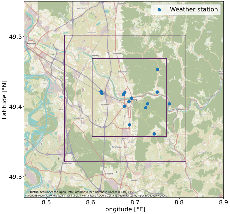
Figure 1The outer box shows the GRAMM domain, which has an extent of 20 km × 20 km with a resolution of 100 m × 100 m. The inner box shows the GRAL domain with a size of 12.3 km × 12.3 km and a resolution of 10 m × 10 m. The blue dots denote the meteorological measurement stations for the matching algorithm. The administrative district borders lie within the GRAL domain and can be seen in Fig. C1 in the Appendix.
In this study, the computational costs are further reduced by utilising a catalogue approach. The catalogue approach exploits the fact that for longer periods similar weather situations reoccur. Utilising the repetition of similar weather conditions, a catalogue of wind fields is computed covering all typical prevailing wind situations for the area. For Heidelberg, we use 1008 synoptic forcings, which are stored and are hourly matched with wind measurements to provide wind fields for the period considered. In particular, during the matching, measured and pre-calculated simulated wind speeds and directions are compared hourly to find the pre-calculated wind situation that minimised the difference with the measurements for that hour. Details can be found in Berchet et al. (2017a, b).
As the lifetime of CO2 is much longer than the period of interest, the concentration enhancement of CO2 in the atmosphere is proportional to the magnitude of the emissions. Using this linearity, a pre-computed concentration field can be scaled linearly to account for a change in the emissions. Emissions from an emission group can be scaled accounting for, e.g. different temporal profiles due to a diurnal cycle of emissions. Note that emission groups do not have to be homogeneous, but may have a sub-structure. However, scaling the emission group then means scaling all emissions in their sub-structure. The total concentration enhancement field for a given time step is obtained as a sum of the concentration fields for each emission group. The choice of the emission groups should reflect the relative variability of the emission sources such that grouped emissions should have a high correlation. The division into emission groups is described in Sect. 2.4.
2.2 The inverse framework
In this study, the inverse problem is estimating emissions x (state vector of length m) from the forward-modelled concentration measurements y (measurement vector of length n). The relation between the measurements and the state vectors, i.e. emission groups per time step, is given by the transport model GRAL
with ϵy as a vector of length n with Gaussian noise characterising the statistical uncertainty of the measurements. Since CO2 is inert on the time scales on which atmospheric transport in the city takes place, the concentration is proportional to the magnitude of the emissions, which means that the model is linear. The Jacobian matrix K (m×n) fully describes the linear forward model and scales the concentration fields for each emission group. Each matrix K for a given meteorological situation is constructed by simulating a concentration field for each emission group xi with i ϵ (1, m). The matrix entries Ki,j are the sensitivities of concentration of a specific measurement yj with j ϵ (1, n) to changes in the emissions of the emission groups:
Depending on the emission scenario, a different linear combination of the emission groups forms the total concentration field of a given hour. As the problem is typically under-constrained and thus no unique solution exists, regularisation is required to obtain a stable and realistic solution. Therefore, we use a Bayesian inversion approach and constrain the solution x by introducing prior emissions xa (vector of length m) and prior error covariance Sa (m×m matrix) following Rodgers (2000):
The uncertainties in y and K are assumed to be Gaussian, unbiased and independent of each other. Sy (m×m matrix) denotes the measurement covariance matrix, which we adjust within the OSSE (see Sect. 3.1). It contains instrument, model and representation errors. We assume that the matrix Sy is diagonal, i.e. has no covariances, implying that the model and measurement errors are not correlated in time and space.
The posterior covariance (n×n matrix) is then given as
For the derivation, see Rodgers (2000).
For multiple time steps, we chain the different atmospheric transport situations by concatenating the matrix K for each time step t of and construct a forward model KT for all time steps, which can be separated into tn independent sets of linear equations if no correlation between states is assumed. The matrices K for each time step are on the diagonal of the new matrix KT as the model GRAMM/GRAL assumes steady-state conditions. This means that the concentration field in an hour depends only on the emissions of the respective hour and not on the hours before. If the atmospheric transport changes from one hour to the next, so will the matrix K.
This equations simplifies and the number of state vectors decreases, if a constant diurnal cycle of the emissions is assumed:
Solving for the posterior emissions requires the prior probability distribution, which is given as a multivariate Gaussian distribution defined by the vector of the mean values for each state xa and the covariance matrix Sa. In the case of uncorrelated states, the prior covariance matrix is with the variances of the state on the diagonal. For correlated states, a common choice of correlation is an exponentially decaying correlation defined by a single parameter per dimension (Kunik et al., 2019). The single parameter defines the strength of the correlation along a distance of a dimension. In principle, the correlation in the prior reduces the total uncertainty of the prior and links the different hours of the inversion making the inverse problem numerically more complex at the same time. We analyse the influence of temporal correlation in the prior of fluxes in Sect. 3.4. The correlation is defined by a correlation strength τt for the time difference between states at the same position. With that, the covariance is
with the standard deviation of state xi at time t0 and time t1 as and respectively.
In Sect. 3.3, we analyse the benefit of measuring CO additionally for estimating CO2 emissions. We assume that they are both passive tracers and thus share the same forward model matrix K. The CO2 emissions can then be expressed in terms of the CO emissions as
with ACO as a diagonal matrix with the flux-weighted mean emission factors αCO per sector with
with xi,s as the CO2 emissions of sector s in flux state vector entry i and αCO,s as the emission factor for sector s. ∑s is the sum over all sectors. We assume the emission factors to be exact for the optimisation in the Bayesian inversion system.
2.3 Evaluation metrics
To describe the properties of the inversion and evaluate the set-ups of the OSSEs, we introduce evaluation metrics, namely the information content, the relative improvement and the root mean square error (RMSE). The metrics evaluate the quality of the inversion (result) and are sensitive to slightly different aspects of the evaluation. Some require the true emissions, while others are able to evaluate the quality of the inversion without knowing the truth. Further, the metrics differ in computational costs. For the analysis, we choose the metric that allows us to best analyse the system and highlight the impact.
First, the information content of the measurement can be derived from the concept of Shannon information, which is similar to the physical entropy (Rodgers, 2000). The Shannon information for the difference of prior and posterior probability for the Bayesian inversion in a linear case and given Gaussian probability distribution is
A denotes the averaging kernel and In is the identity matrix with dimension n. For details on the concept and derivation, see Rodgers (2000). One can see that the information content increases with the averaging kernel getting close to identity. The information content describes the quality of the set-up independently of the actual difference between the prior and the truth. It can therefore be used as a measure for the quality of the inversion, in which the truth is not known. Since it is a scalar quantity, it is useful for optimising observing systems as well as characterising and comparing them. However, in an OSSE, the truth is known, such that the difference between truth and posterior emissions can also be used for evaluation of the set-up. The RMSE over the entire domain is defined as the difference between the sum of the two vectors and .
The RMSE of the total fluxes gives quantitative information on how close the total posterior flux is to the true total in the domain. In contrast to the information content, it does not capture the complete probability distribution, but rather the effect of the stochastically generated noise. However, it is computationally cheaper to calculate. Additionally, the relative improvement can be calculated, if the true emissions are known:
with xa the prior flux, the posterior flux, and x* the true emissions. The relative improvement scales the difference between the posterior and the truth of each state by the difference between the prior and the truth of the states. The relative improvement is 0 % if the RMSE of the posterior has not improved compared to the prior and 100 % if the posterior and the truth are identical.
2.4 Emission data and uncertainties
In this study, we simulate anthropogenic CO2 enhancements. In the following, we explain the data sets used to construct the true emissions as well as the prior for the inversion. The fluxes of the inventories have a high resolution (see Sect. 2.4.1 and 2.4.2), but we group the fluxes into emission groups, which we use as basis vector for the inversion. The emission groups are administrative districts from OpenStreetMap. Therefore, only the total emissions per administrative district are optimised for, even though a district still exhibits a higher resolved sub-structure. While there are actually 26 administrative districts, small districts and districts at the domain border have been aggregated (see Fig. C1) such that there are 19 districts which can be optimised. The reason for choosing administrative districts is that the emission information should meet the needs of the stakeholder (Jungmann et al., 2022) and should be well constrained by a reasonable number of sensors. For Heidelberg, administrative districts are a politically meaningful unit exhibiting an area large enough to be constrained with a realistic number of sensor nodes. We choose to aggregate smaller districts and border districts as they are very difficult to constrain because they contribute only weakly to an overall enhancement. To assign area emissions on a district level, area sources are interpolated to the GRAL grid of 10 m × 10 m and each pixel on the GRAL grid is assigned to the district with the maximum overlap.
2.4.1 True emissions
For the true emissions, we use data with a high spatial and temporal resolution to reflect the expected heterogeneity and variability of the emissions in the urban area. Traffic emissions were taken from a OpenStreetMap-based emission estimate (Ulrich et al., 2023) as line sources with street-resolving (3 m) resolution. Combustion emissions are based on data for the yearly consumption of natural gas, fuel, oil, liquid gas, coal, wood and pellets in the municipality of Heidelberg, as provided by the public utility company of Heidelberg (“Wärme Atlas 2017 Aggregation”, version 001). The emissions are primarily caused by residential heating and do not include traffic emissions. The combustion data are aggregated on a grid with a resolution of 100 m × 100 m to protect the privacy of the customers. For the same reason, if there are fewer than five customers in a single grid cell, the data are masked and not available in the inventory. We treat masked emissions as if they do not contribute, i.e. set these grid cells to zero. Finally, the remaining emissions from Gridded Nomenclature for Reporting (GNFR) sector G to L are additionally accounted for as true emissions. We use the area emissions provided by TNO (Nederlandse Organisatie voor Toegepast Natuurwetenschappelijk Onderzoek) as true residual emissions. However, these area emissions contribute only 1.4 % to total emissions (see Table 1). All true emissions are then cut into administrative districts for division into base vectors (see Fig. C1), but still have a sub-structure, as described above and as illustrated in Fig. 2.
There are only two TNO point sources in the GRAL domain which are each treated as an individual group. The two TNO point sources in the domain are emitted as point sources at stack heights of 85 and 120 m. A fixed diurnal and weekly cycle of emissions is assumed following the profiles listed for each GNFR sector by Denier van der Gon et al. (2011).
2.4.2 Prior emissions
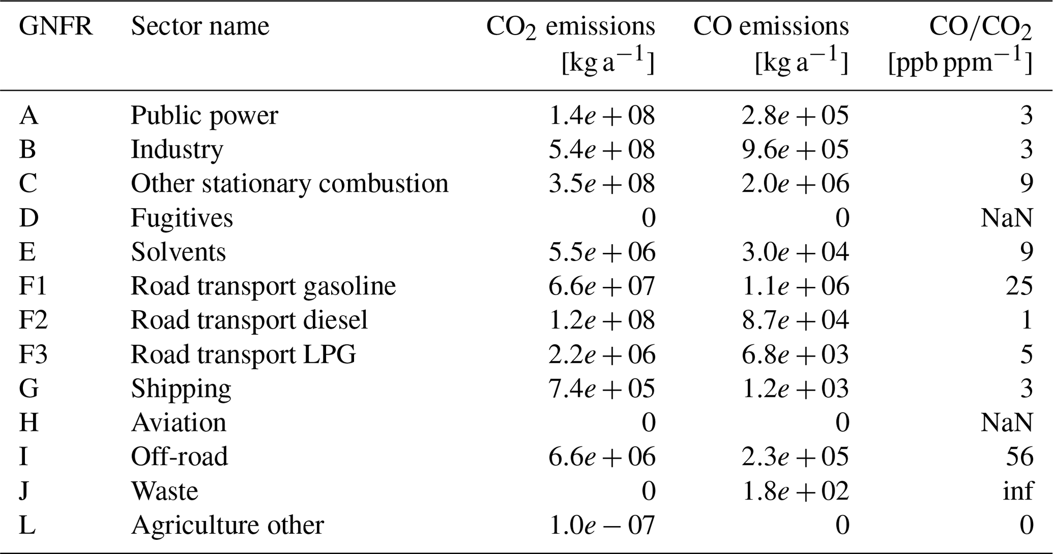
We use emission data from the TNO inventory (Super et al., 2020) as starting point for constructing the prior. The data set consists of an inventory of area sources with a resolution of longitude × latitude (≈1 km × 1 km over Central Europe) and point sources. TNO emissions are shown for the Heidelberg GRAL domain in Fig. B1. While the data set consists of 10 different emission maps which were constructed with a Monte Carlo approach, only the first realisation of the set is used. Emissions are divided into emission categories according to the GNFR category for both CO2 and CO. From this, the mean emission factor for each GNFR category for the entire GRAL domain is obtained. The emissions and ratios for the Heidelberg domain are listed in Table 1 and are used in Sect. 2.4.
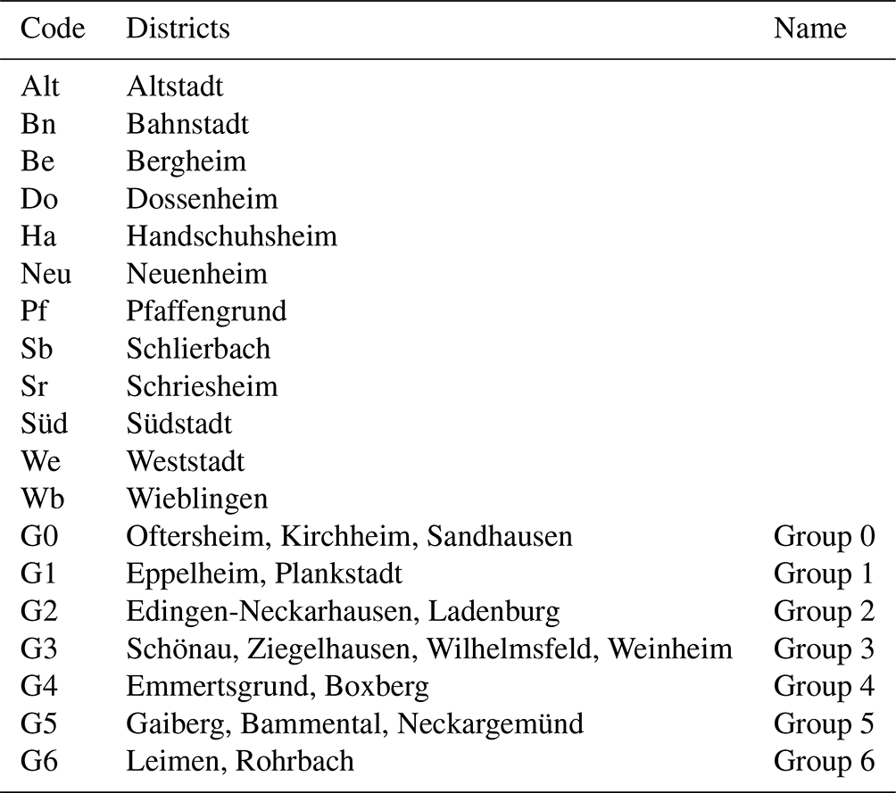
Table 1CO2 and CO emissions per year in Heidelberg and ratio of [ppb ppm−1] for different Gridded Nomenclature for Reporting (GNFR) emission sectors as taken from TNO (Super et al., 2020). The ratio was calculated by converting from kilograms to parts per million (ppm) or parts per billion (ppb) by taking into account the molecular mass of CO and CO2. The GNFR sectors are the basis for reporting spatially distributed emissions of air pollutants by European countries.
TNO area emissions are divided into administrative districts as described above. We further smooth out the area TNO emissions such that the mean emissions per area are equal for each district; however, they are not constant over the domain because emissions per area still exhibit a sub-structure within the district (see Fig. 2). The prior emissions are set constant in time and do not have a diurnal cycle. The reason for introducing smoothing across districts, as well as the constant temporal profile for the prior, is to reflect a realistic difference between prior and truth that would also be expected in a real inversion. In addition to the area sources, the TNO point sources are also accounted for in the prior.
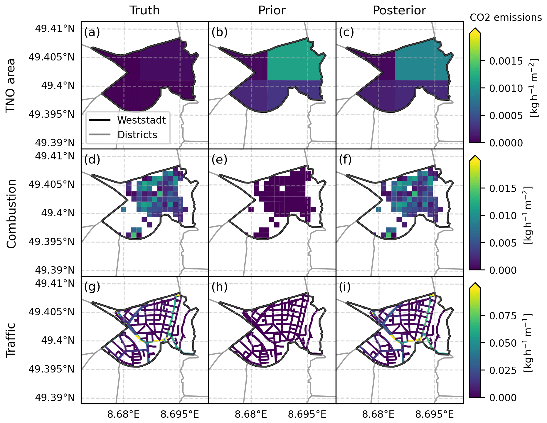
Figure 2For the city district Weststadt (“We”) three elements of the state vector are shown (three rows). The columns show the true, prior and posterior emissions for TNO area emissions (a, b, c), combustion emissions (d, e, f) and traffic emissions (g, h, i). This plot illustrates three of the state entries seen in Fig. 3. Note, that the prior (d, e, f) for combustion and traffic is zero, but exhibits the fixed sub-structure of the truth. The combustion emission in the district exhibits white 100 m × 100 m squares, which are masked due to data protection policy. The posterior emissions differ depending on the data assimilated and are illustrated here for 10 CO2 measurements in the entire Heidelberg domain with 1 ppm uncertainty. Posterior results are discussed in Sect. 3.
The prior uncertainties for TNO point and area sources are set to 100 % of the prior flux. Prior uncertainties for traffic and combustion sources are set to 100 % of the true emissions since the prior emissions for traffic and combustion sources are zero.
In total, there are 59 emission groups consisting of two point sources, and 19 districts with emissions from the TNO area sources, the traffic simulations and the combustion data. This choice of emission groups defines the dimension n of the inversion framework. Figure 2 illustrates the three emission groups (area, combustion and traffic) belonging to the district Weststadt. The temporal mean emission strength of all emission groups is illustrated in Fig. 3 for prior, prior uncertainty and truth.
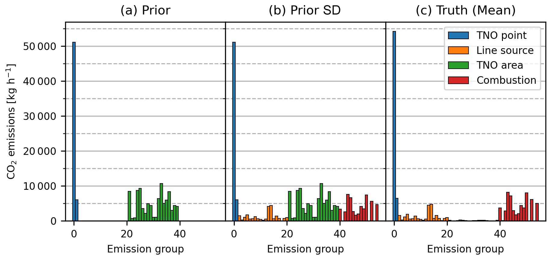
Figure 3Emissions of each state vector for prior (a), uncertainty of the prior as the standard deviation (SD) (b) and truth averaged over time (c). The different emission groups contain emissions from the TNO point (blue) and area sources (green), the traffic simulations (orange) and the combustion sources (red).
Note the differences between the magnitude of the emission groups in the prior and the truth. As the prior and true emissions are accounted for in different emission groups, corresponding to different vector entries in state x, the inversion needs to redistribute to the other source types to correctly estimate sectoral and spatial patterns. This configuration pushes the limits of the current inversion set-up as it tests the capabilities of the inversion system to identify spatially overlapping emission groups. For the entire domain, prior and true emissions differ on average by 13.5 % ((truth–prior)truth).
2.5 Inversion experiments
This study examines the performance and design parameters of a network of sensors that measure the CO2 concentration in air in an urban environment by combining a high-resolution atmospheric transport model on building-resolving scale with an atmospheric inverse model. The investigation focuses on various aspects to gain initial insights into the capabilities of a monitoring network in Heidelberg. To systematically analyse different parameters of a measurement network, we conduct four separate experiments, each targeting different aspects of network design or inversion set-up. We analyse the number of sensors versus the quality of sensors (Sect.3.1), the optimal horizontal sensor placement (Sect. 3.2), the benefit of utilising CO as an additional tracer (Sect. 3.3) and the effect of introducing a temporal correlation in the prior error covariance (Sect. 3.4). In all experiments, the virtual sensors, which “sample” the atmospheric trace gas concentrations, are placed at 2 m above ground level and positioned such that they form a rectangular grid that covers the domain. Then, either all sensors are used or they are sub-sampled from the grid as described for each respective experiment in Sect. 3. The grid is chosen as a first approach to find the optimal sensor placement. The inversions are performed for wind situations during the period of 22 July 2021 to 21 August 2021. For the experiments in Sect. 3.1–3.2, 24 random hours are sampled from the first 300 h of the period. For the experiments in Sect. 3.3–3.4, the first consecutive 120 h (5 d) of the period are used for the inversion to test whether the posterior estimate captures the correct temporal pattern. For the inversion, we assume constant emissions in Sect. 3.1–3.2 and a fixed diurnal cycle as described in Sect. 2.4 for Sect. 3.3–3.4. In the OSSE conducted, the influence of biogenic CO2 fluxes and background concentrations is not considered. Instead, the simulated concentration fields specifically represent the increase in CO2 concentration resulting from anthropogenic fluxes within the domain. This simplification corresponds to periods when biogenic influences in the city centre are very small, most likely in winter, and exact background estimations of CO2 transported from outside the domain into the domain are available. Both assumptions are not valid during most parts of the year. However, the goal of this OSSE is to evaluate the inversion framework and analyse the sensitivity of network configurations to CO2 emission estimates as a starting point for optimal network design in Heidelberg. As such, we do not claim completeness. We elaborate on the limitation caused by these simplifications in Sect. 4.
3.1 Sensor quality and quantity
The optimal design of a measurement network is constrained by the total costs of the network limiting quantity and/or quality of the sensors and transport model used. In this experiment, the quality of the inversion is investigated for different numbers of sensors with different mismatch errors Sy. The mismatch error includes instrument errors, model errors as well as representation errors. While all of the errors are inevitable, the instrument errors deserve special focus as this is a design variable for building a monitoring network. High-cost sensors have better precision than mid-cost or low-cost sensors, but are much more expensive such that we expect a trade-off between quality and quantity for a given budget. We follow the set-up by Turner et al. (2016) and conduct multiple Monte Carlo experiments, each with N=2000 runs. In a Monte Carlo experiment a model variable, in our case sensor location, is sampled randomly to estimate the probability of having a certain outcome, in our case of having a certain information content of the inversion. We place 5, 10, 15, 20, 25 and 30 sensors randomly on a 5 × 6 grid within the domain (30 possible locations) with a total noise of 0.1, 0.5, 1.0, 2.0, 3.0, 4.0, 5.0, 10.0 ppm. We conduct the analysis for 24 randomly selected wind situations. For illustrative purposes, Fig. 2 plots the true (left column), prior (middle column) and posterior emissions (right column) for the district “Weststadt” on a map for the three emission groups, namely for area emissions (upper panel), combustion emission (middle panel) and traffic emissions (lower panel). One can see that an emission group is not flat, but exhibits a sub-structure. Posterior emissions are shown for a specific setting (10 CO2 measurements with 1 ppm uncertainty). The mean posterior result for each state (all districts, all sectors, same setting) can be seen on the left in Fig. 4.
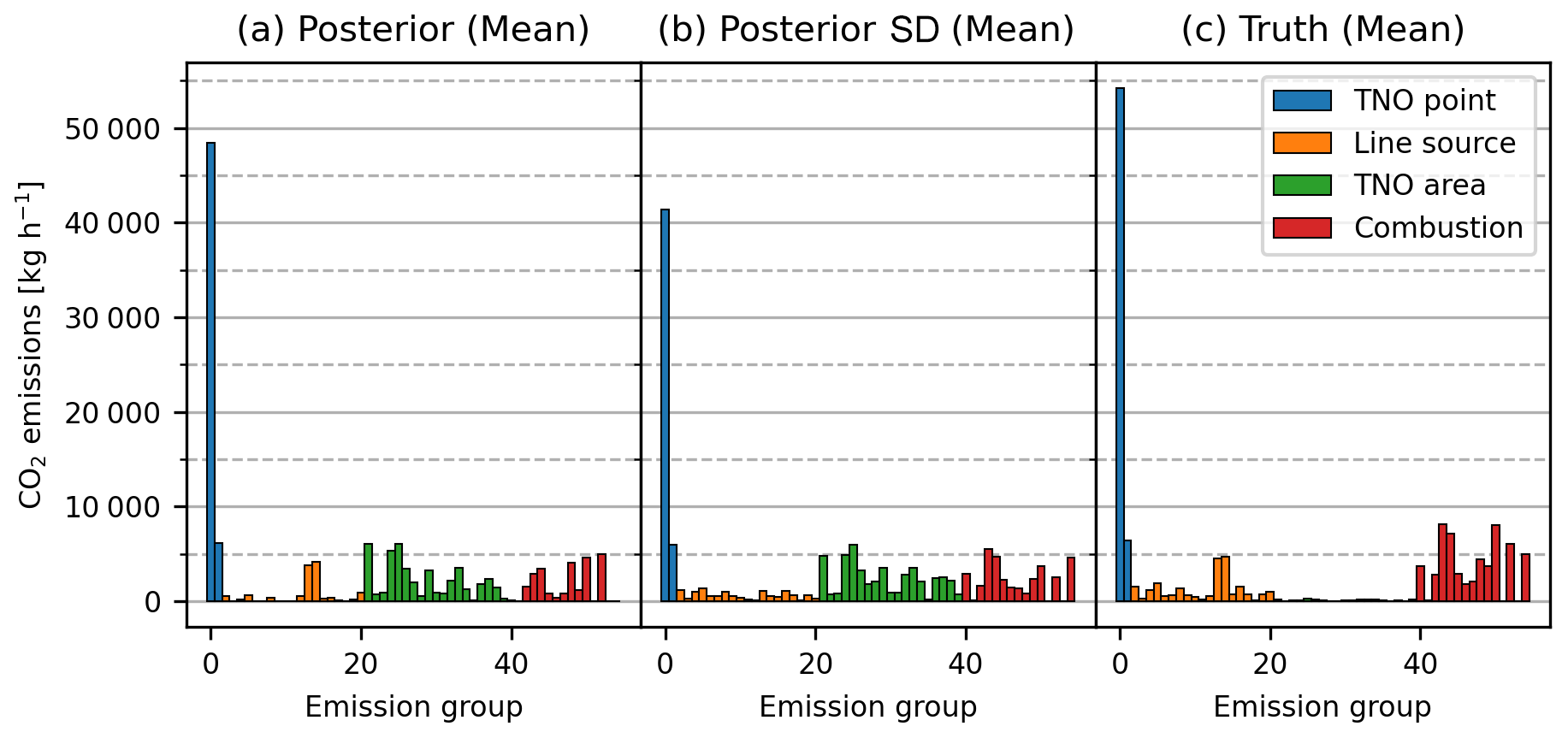
Figure 4Mean posterior emissions of each state vector (a), mean posterior uncertainty (b) and true emissions of each state vector (c). The different states refer to emissions from the TNO point (blue) and area sources (green), the traffic simulations (orange) and the combustion sources (red). Note that the prior emissions and uncertainties are given in Fig. 3.
For quantitative analysis of the optimal configuration, Fig. 5 shows the relative improvement of the estimation of the city-wide emission flux for the different sensor noises and number of sensors. The relative improvement increases with quantity and with the decrease in model–data mismatch error, e.g. by increasing the quality of sensors. Similar to Turner et al. (2016), we can identify noise-limited configurations (e.g. 25 sensors at 2 ppm uncertainty in Fig. 5) for which the flux estimation improves more by increasing the quality of the sensors and models and site-limited configurations (e.g. 5 sensors at 2 ppm uncertainty in Fig. 5) where the flux estimation improves more by increasing the number of sensors. While the quality of flux estimation increases with the number of sensors and sensor quality, the budget for a sensor network is limited. The best choice of network depends on the monetary constraints for the sensor network and the costs of each sensor.
The plot allows us to compare the relative improvement of flux estimation for different networks in Heidelberg. One can then utilise Fig. 5 to identify the configurations that are still affordable (subset of squares in Fig. 5) and find the configuration that maximises the relative improvement of the flux estimation. This implies that for any given budget one can base a decision regarding whether to invest in more or in better sensors (and models) on these results. Note that here we only account for a random uncertainty in sensor noise assuming uncorrelated measurement uncertainties among sensors. We do not analyse systematic errors within the measurement network, which could be present because of, e.g. temperature-dependent drifts of the sensors (Delaria et al., 2021) or by a background transport errors. Although analysing systematic offsets was not the scope of this study, the inverse framework established can be easily used to study such effects in the future.
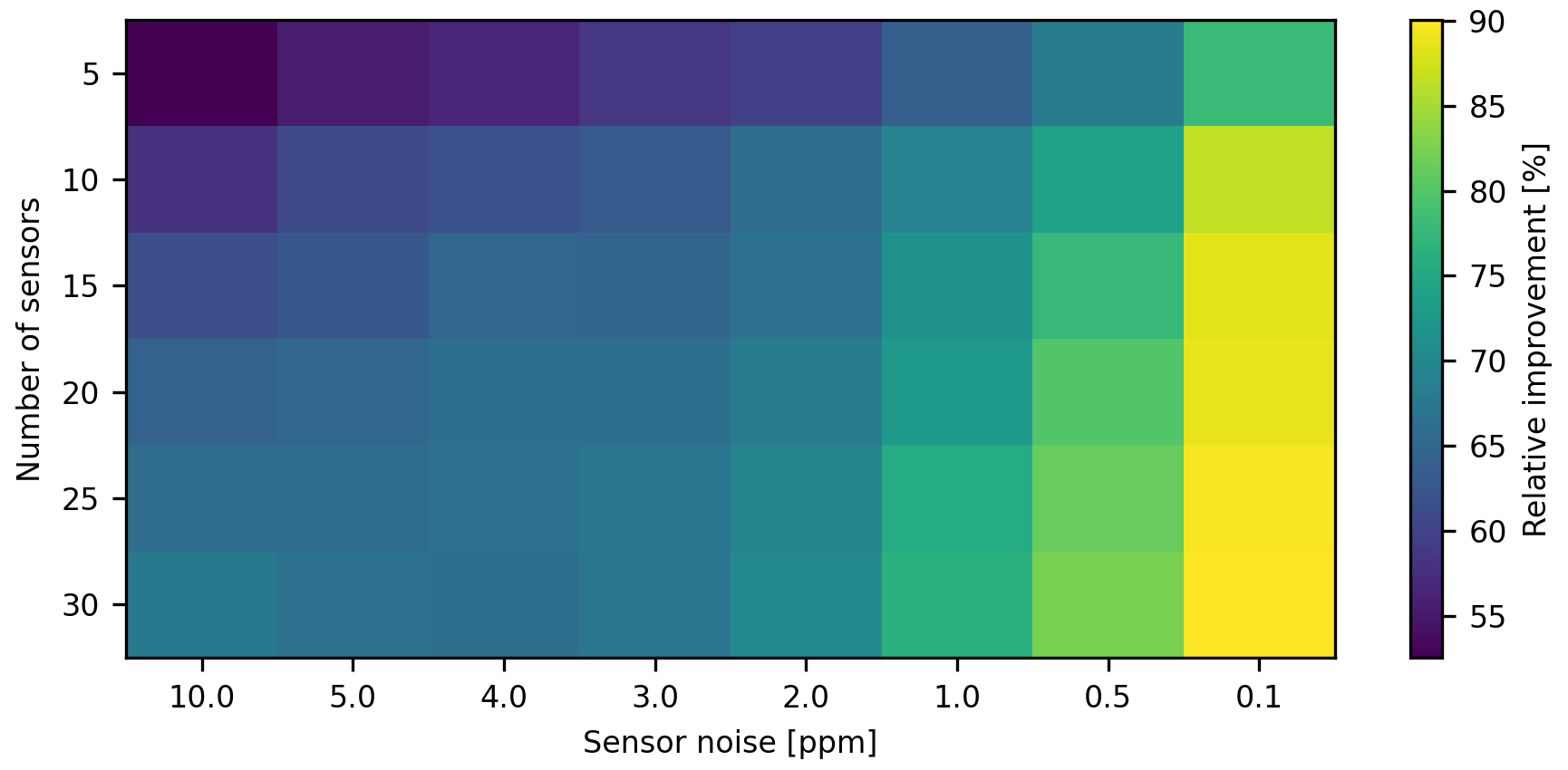
Figure 5Relative improvement of the flux estimate for different configurations of the number of sensors and the measurement error of the sensors. The relative improvement increases with increasing number of sensors and sensor noise.
3.2 Sensor placement
In Sect. 3.1 we randomly sub-sampled a number of sensors from a 5 × 6 grid. Now, we analyse the optimal spatial distribution of the sensors. We therefore compare the sensor placement in a regular grid with a random selection of locations in the domain. For the random selection, we run Monte Carlo simulations (each N=2000) for different sensor numbers again using 24 randomly selected wind situations and offering 100 (10 × 10 grid) different possible sensor positions at 2 m above ground. We analyse the information content for 9, 16, and 25 sensors for the random placement and for a regular grid placement assuming a measurement precision of 1 ppm (see Fig. 6). One can clearly see that the information content increases with the number of sensors, as expected since more sensors offer better information on the emissions. On average, the grid placement outperforms the random placement as can be seen from the mean values in Fig. 6. This means that without further information on the underlying emission statistics, it is beneficial to place the sensors in a regular grid rather than placing them randomly. This is expected since a regular grid covers the entire domain and therefore is less likely to be insensitive to emissions from specific areas. The difference between random and grid placement, as well as the distribution of the random placement, is especially large for a low number of sensors. For a low number of sensors, the random placement of sensors is more likely to be spatially heterogeneous and therefore may be especially well or badly placed contributing to lower and higher information content than in the random placement. The distribution of information content for the randomly placed sensors decreases for a higher number of sensors due to a better statistic. Interestingly, the placements with the highest information content are again random placements. We analysed the right tail (10 best-performing sensor arrangements) of the random distribution of nine sensors with high information content. Figure 7 shows the locations of the configurations with the highest information content. The locations with large incident number produce high information content in many meteorological situations and should therefore be considered as optimal location for a measurement network. As the tail of the distribution corresponds to individual realisations of the Monte Carlo experiments, it remains unclear whether the “high information content tail” is driven by a specific set of wind situations or whether these measurement locations outperform the grid placement in all wind situations. For our Heidelberg setting, one can see that the measurement locations providing the most information content are located in the city centre and in the vicinity of higher emissions. In the east of the domain, which is dominated by forest areas with low anthropogenic CO2 emission in the true emissions, only few sensors are placed. In future work, we plan to extend this study by considering also measurement stations at higher altitudes above ground since higher stations are less influenced by local sources and are therefore likely to provide information on the emission patterns over a larger area. This might be complementary to the ground-based sensors.
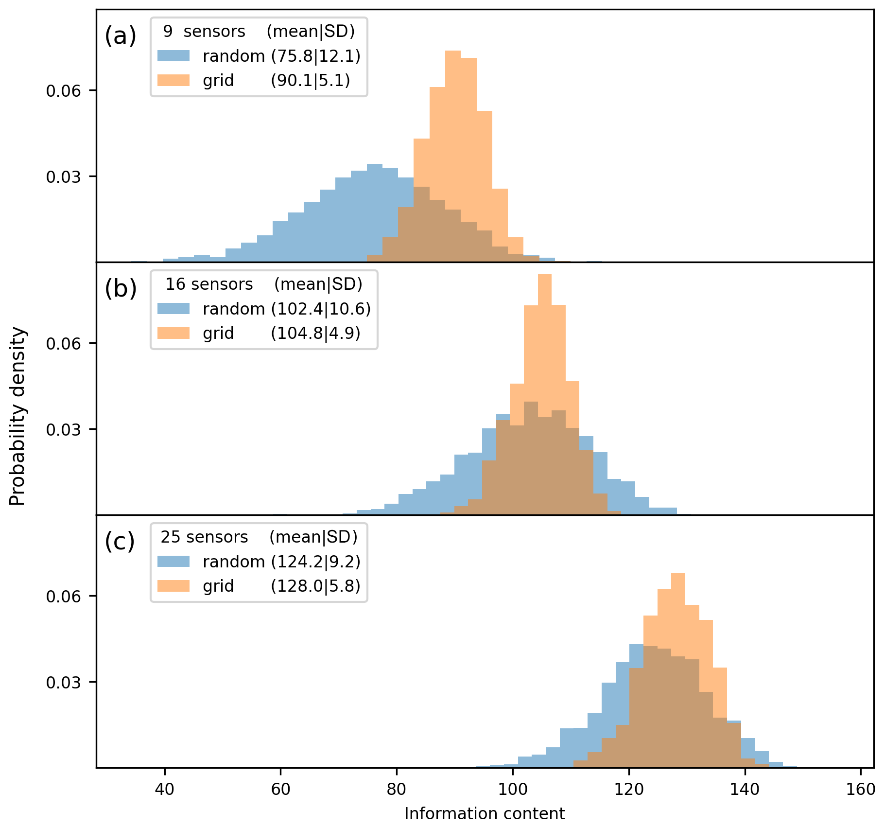
Figure 6Information content distribution for the inversion set-up for varying wind conditions. The information content increases with the number of sensors from (a) to (c). The mean information content of randomly placed sensors (blue) is higher in the grid placement, but as the standard deviation of the random placement is larger, the highest information content is achieved for some configurations with randomly placed sensors.
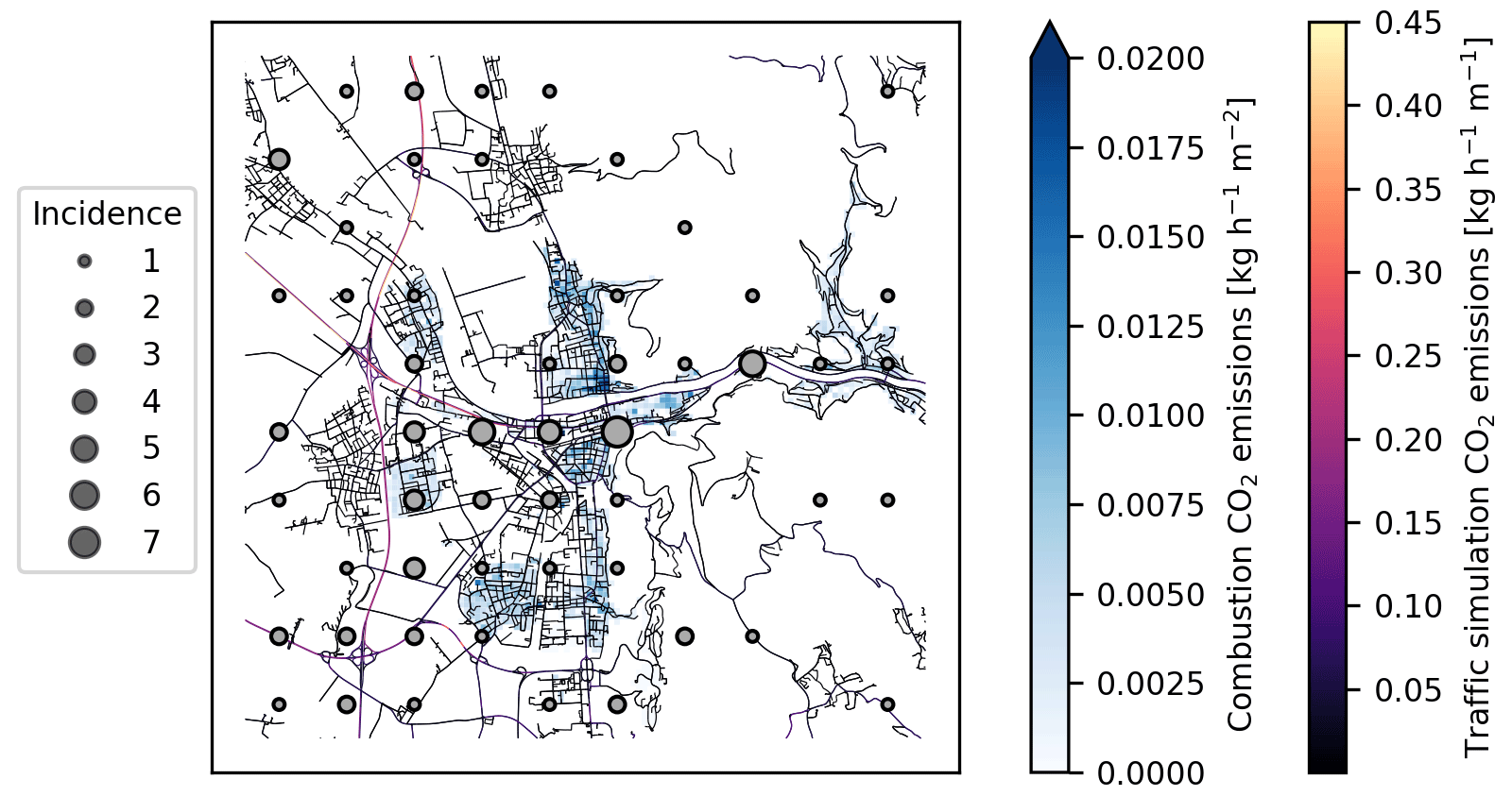
Figure 7Sensor positions of the 9 sensors with the 10 highest information content. The size of the dots indicates the incidence of the sensor position of the 100 available positions in the experiment.
3.3 CO as additional tracer
CO is co-emitted when burning fossil fuels. Depending on the source type, the ratio of the emissions differs (see Table 1). As CO and CO2 are nearly passive during 1 h, both tracers are transported linearly with the same atmospheric transport. Therefore, measuring the atmospheric CO concentration can provide additional information about the specific emission groups and potentially also about the total CO2 emissions in general as both stem from anthropogenic sources. We now analyse to which degree the estimation of CO2 emissions benefits from measuring CO enhancement as an additional tracer along with CO2. Note that we neglect biogenic CO emissions, which are normally expected to be much smaller than anthropogenic CO emissions in cities. While the mean ratio of all anthropogenic sources in Heidelberg is 5 ppb ppm−1, it is about 10 ppb ppm−1 for traffic emissions (see GNFR sectors F1–F3 in Table 1) making CO measurements especially sensitive to traffic emissions.
In this experiment, we assume that all measurement stations measure both CO2 and CO with uncorrelated measurement errors of 1.0 ppm for CO2 and 2.0 ppb for CO. The inversions are performed for a period of 5 d and the diurnal cycle is assumed to be identical for each day. We conduct this experiment using 10 sensors. The prior is constant during the period and we do not introduce any correlation into the prior.
Figure 8a shows the total anthropogenic CO2 emissions during the course of the day. While the prior is constant in time, the truth actually shows a temporal profile with distinct morning peak. One can see that both inversion results (posterior with CO2 only and with CO2 and CO) differ from the flat prior and are able to capture the profile of the true total emissions. In the given setting, there is no significant improvement in the posterior emissions of total CO2 when including CO in the inversion. Note that this finding only holds in our setting when neglecting biogenic emissions. However, for future studies, we encourage re-analysing the benefit of CO for total anthropogenic CO2 when including biogenic emissions. Figure 8b shows the traffic emissions. Again, both posterior inversions differ from the flat prior emissions. However, the posterior estimate using the CO as additional constraint in the inversion is much closer to the true emissions. The same is true for combustion emissions (see Fig. 8c). This means that in our setting, for the given emission ratios and measurement uncertainties, the additional measurement of CO is useful in the inversion to separate different emission groups.
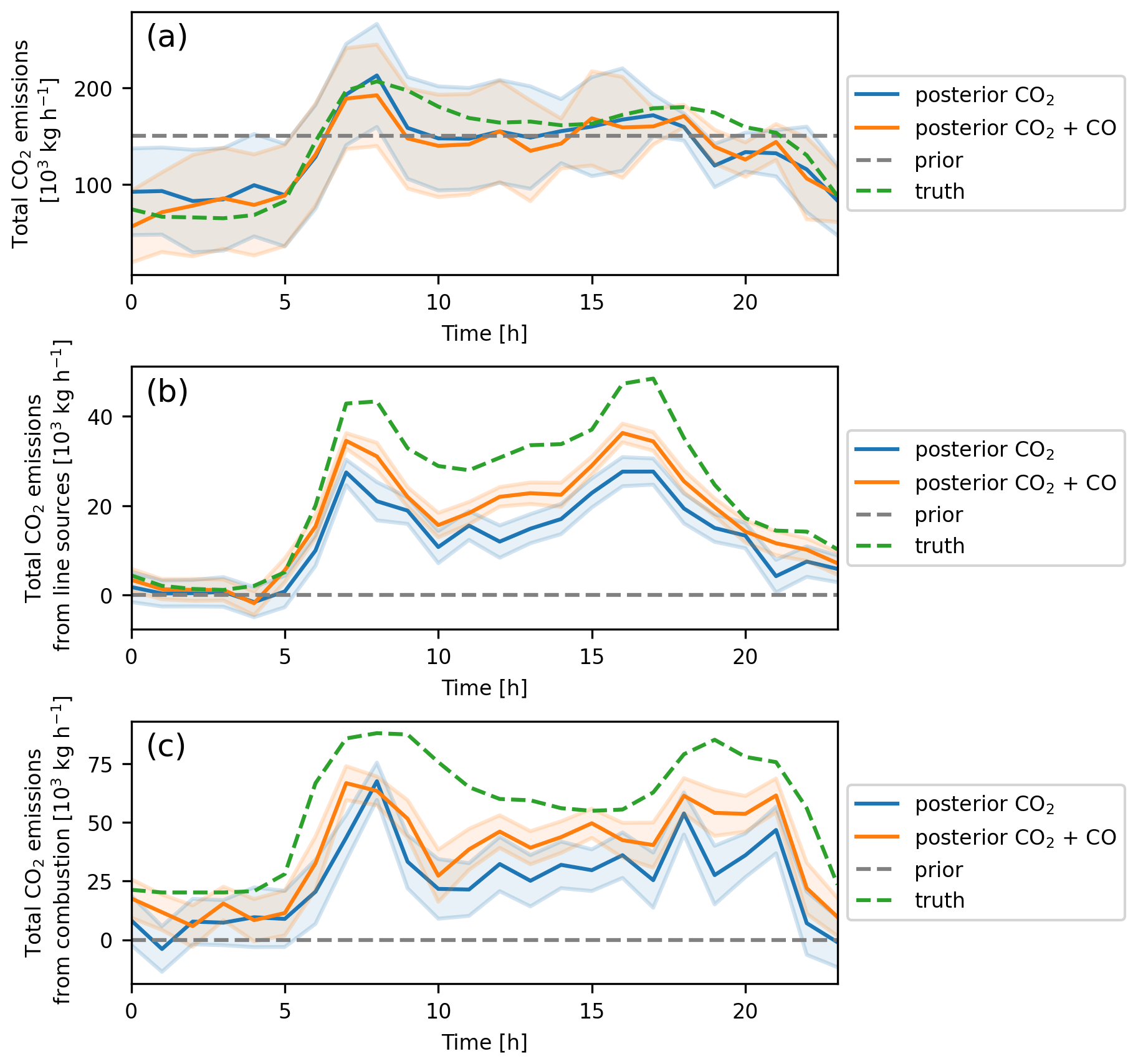
Figure 8(a) Diurnal cycle of the total CO2 emissions in Heidelberg. The figure shows the posterior for an inversion utilising CO2 only (blue) and an inversion utilising CO2 and CO (orange). The shaded area is the standard deviation derived from the posterior covariance. The dotted lines show the prior emissions (grey) and the truth (green). (b) Same as (a), but for traffic instead of total CO2 emissions. (c) Same as (a), but for combustion emissions.
3.4 Temporal correlation of the prior
In the previous sections, we retrieved the CO2 emissions for every hour without assuming any correlation between the states. Without temporal correlation, each hour of the inversion is independent of the previous and the following hour. We now examine the effect of considering temporally correlated states to reflect the existence of temporal emission trends exceeding 1 h time scales. A correlation in the prior reduces the total uncertainty of the prior. However, the choice of the correct correlation length is vital. A larger correlation length leads to a smoothed time series, as measurements inform multiple emission states and thus exhibit a larger corrective power over neighbouring hours. On the other hand, smaller correlation lengths can better account for spikes during the measurements. The choice of optimal correlation length therefore depends on the underlying emission patterns.
In the first analysis, we varied the correlation length τh and analysed how the RMSE of the CO2 emissions for different emission groups changes with correlation length (see Fig. 9). This analysis is only possible in an OSSE when the truth is known and an RMSE can actually be determined.
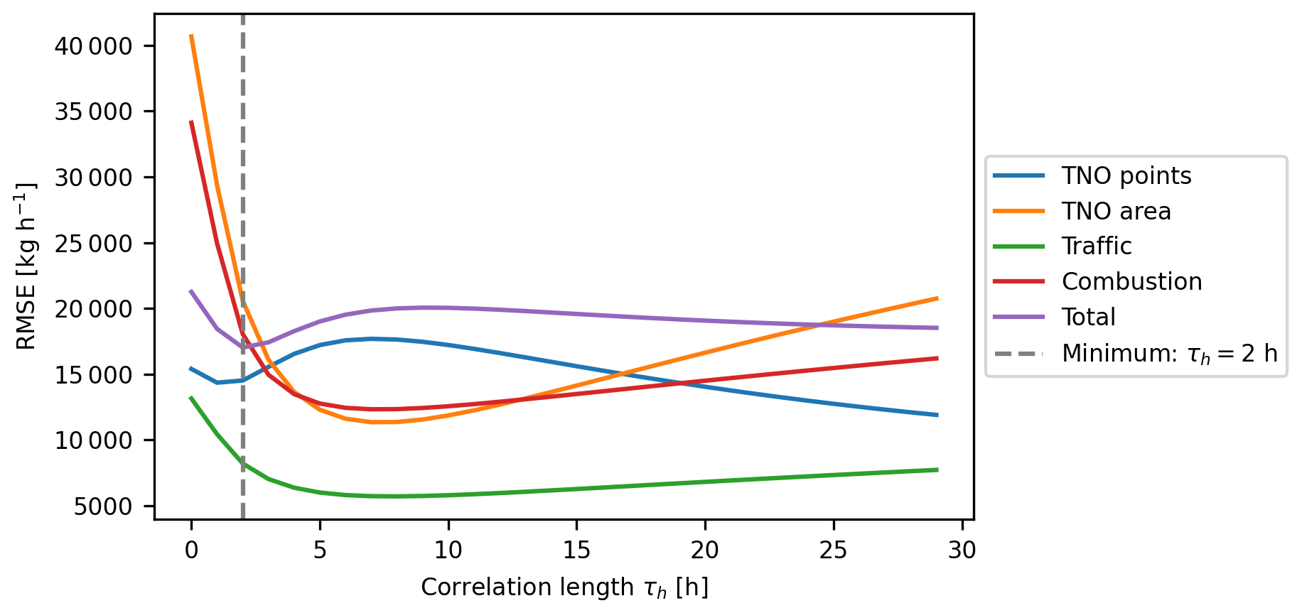
Figure 9RMSE of the different emission sources for different correlation lengths τh. The dashed grey line indicates the minimum of the RMSE for the total emissions, which is at a correlation length of 2 h.
As the optimal correlation length depends on the temporal emission dynamics, it is also dependent on the source type. Focusing on the total CO2 emissions, we find a clear minimum for about 2 h. This is driven by a shorter optimal correlation length for point sources and longer optimal correlation lengths for traffic, heating or other area emissions. The curve for the point sources, which are emitted at heights of 85 and 120 m, is qualitatively different from the curve of the ground-based sources. While introducing any correlation time has a positive effect on the RMSE for ground-based sources, the effect can be detrimental for point sources. For point sources, correlation times between 4 and 15 h are too strong for our setting. Here, we chose the 2 h as correlation strength to estimate posterior emissions and highlight the importance of choosing the optimal correlation time especially for determining point sources. In Fig. 10a we analyse the benefit of using a posterior correlation of 2 h to estimate total CO2 emissions. The estimation of total CO2 emissions improves when introducing the prior correlation. While the benefit is only small for total CO2 emissions, the traffic and combustion emissions improve substantially when introducing a prior correlation (see Fig. 10b and c). This finding for our OSSE in Heidelberg is in accordance with the results from Kunik et al. (2019) for Salt Lake City. This shows that it is beneficial to introduce a temporal correlation of the prior states if underlying emission dynamics are temporally correlated, since neighbouring states can inform and correct for each other.
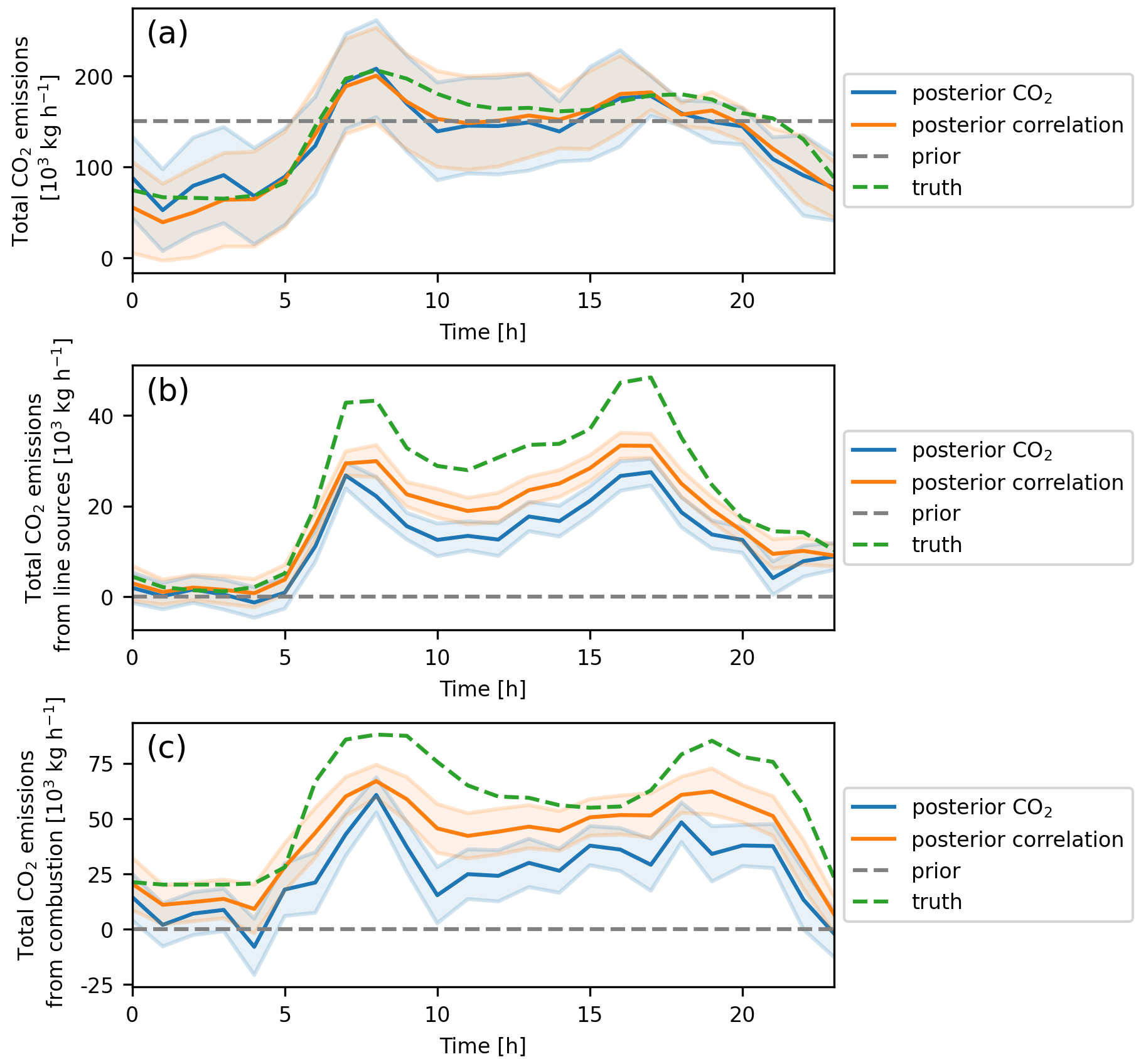
Figure 10(a) Diurnal cycle of the total CO2 emissions. The figure shows the posterior for an inversion with uncorrelated prior emissions (blue) and with time-correlated prior emissions with a correlation length of 2 h (orange). The shaded area is the standard deviation derived from the posterior covariance. The dotted lines show the prior emissions (grey) and the truth (green). (b) Same as (a), but for traffic instead of total CO2 emissions. (c) Same as (a), but for combustion CO2 emissions instead of total CO2 emissions.
In this set of experiments, we analyse the trade-offs inherent in balancing sensor quantity and sensor quality, we determine the optimal sensor locations and we evaluate the advantages of measuring CO along with the impact of introducing temporal correlation into the inversion framework. These investigations are conducted within a simplified urban setting in Heidelberg.
The information content and, consequently, the precision of emission estimates depend on both the quantity and quality of the sensors deployed. The potential accuracy of flux estimation increases with an increased financial budget, enabling the installation of additional or superior sensors. Through our experiments, we are able to determine the optimal sensor configuration – considering both quantity and quality – tailored to any given financial constraint.
The experiments further suggest locations of preferred sensor installation based on Monte Carlo simulations. The GRAMM/GRAL model proves especially advantageous for assessing optimal sensor positions due to the storage of full-concentration fields for each wind situation. Other models often compute footprints for predefined sites, which makes the analysis of a large number of possible sensor locations less efficient. We analyse the performance of a network with equally spaced sensors versus randomly placed sensors inside the domain. On average, equally spaced sensors outperform randomly placed sensors. This means that in the absence of information on the emission distribution, an equally spaced sensor placement is a good starting point. However, there are network configurations that yield better performance in terms of emission estimates, particularly when located near emission sources and in the centre of the domain.
Moreover, we assess the advantages of incorporating CO as an additional tracer. Although CO measurements do not significantly enhance the overall estimation of total CO2 emissions in this setting, they do contribute to an improved estimation of sector-specific emissions. The limited impact of including CO for the estimation of total CO2 emissions can be attributed to the absence of biogenic emissions in the presented setting. Consequently, the total CO2 emissions are already well represented by sampling the total simulated CO2 enhancements. In reality, the total CO2 enhancement, in contrast to total CO enhancement, is significantly influenced by biogenic sources – especially in spring and summer. Reassessing the benefit of CO as a tracer for anthropogenic CO2 is therefore encouraged after including biogenic emissions into the framework. Beyond that, it is possible to adjust ratios of different sectors to mimic anticipated changes in ratios, and evaluate the benefit of the tracers under these circumstances again.
Finally, we analyse the influence of the prior probability distribution on the inversion by introducing a temporal correlation in the prior emission estimate. The introduction of temporal correlation increases the overall uncertainty reduction. The optimal correlation length is source dependent, but it is 2 h for the total emissions in our setting. Using this correlation length improves the emission estimate and minimises the discrepancy between the posterior emission estimate and the true emissions, which again is in line with previous studies.
The results provide an initial indication on how to construct a network and beyond that they show the principal applicability of GRAMM/GRAL in an inversion framework. However, all results still exhibit uncertainties due to various aspects: first, like any model, GRAMM/GRAL exhibits transport errors. The performance of GRAMM/GRAL has been assessed in multiple studies and has to be taken into account in the inversion (as model–data mismatch). Utilising a wrong error for the model transport may distort the outcome of the inversion. The same argumentation holds for instrumentation errors. So far, we have only considered random noise for the model–data mismatch. However, the framework makes it possible to evaluate systematic biases, e.g. due to sensor drifts or emissions transported from outside the model domain to the sensor locations.
Second, introducing biogenic emissions and analysing the effect of background concentrations is essential for drawing final conclusions on the design of the measurement network in urban areas. Biogenic emissions enhance the total CO2 signal and thus mask the contributions from anthropogenic sources. The effect of CO2 transported into the model domain will be larger the smaller the domain. In Heidelberg, we expect the effect of transported emissions to be considerable as emissions from the city of Mannheim influence the concentrations in Heidelberg for typical west-wind situations. The magnitude of concentration enhancement and its effect on the emission estimation still needs to be explored in future work. However, there are possibilities to account for the transported emissions – either by setting up dedicated measurement stations at the domain borders or by including an uncertainty for the background enhancement into the inversion framework, which will be explored in a next-generation OSSE for Heidelberg.
Third, the choice of state vector will influence the result. In future, one might consider changing from emissions grouped into districts with fixed sub-district variation to, e.g. a high-resolution regular grid. This would decrease the aggregation error and account for finer spatial dynamics. However, as this increases the dimension of the state vector, more measurements will be necessary to determine the fluxes on higher resolution equally well.
While an OSSE will never be able to mimic the real world fully, approaching realistic settings in the model world is important in order to obtain the correct indications for sensor network planning. Using the framework presented here, we can now add further complexity and conduct numerous additional experiments, such as exploring moving sensors, incorporating additional tracers, analysing different sensor heights and extending to longer time periods.
We have developed a framework for conducting OSSEs using the high-resolution transport model GRAMM/GRAL. This framework allows us to perform various experiments to assess the capabilities and sensitivity of a measurement network to specific parameters.
The developed framework represents the first step towards conducting atmospheric inversions using a transport model with a resolution considerably below the kilometre scale. The experiments enable comparisons between different network parameters and therefore optimisation of the network design based on high-resolution transport. We have demonstrated the feasibility of estimating CO2 emissions for Heidelberg at a district level and give the first indications for sensor network design. The main advantage of using GRAMM/GRAL in the inversion lies in the cost-effective forward model employed in the catalogue approach, as well as the assumption of hourly steady state in the model. This steady-state assumption enables easy determination of the Jacobian required for inversion. This advantageous characteristic facilitates network optimisation across various parameters and locations, even encompassing areas influenced by street channelling and buildings. This framework provides the basis for efficient estimations of high-resolution CO2 fluxes in an urban setting. In the next step, we can further enhance the realism of the OSSE by incorporating additional complexities.
Prior emissions
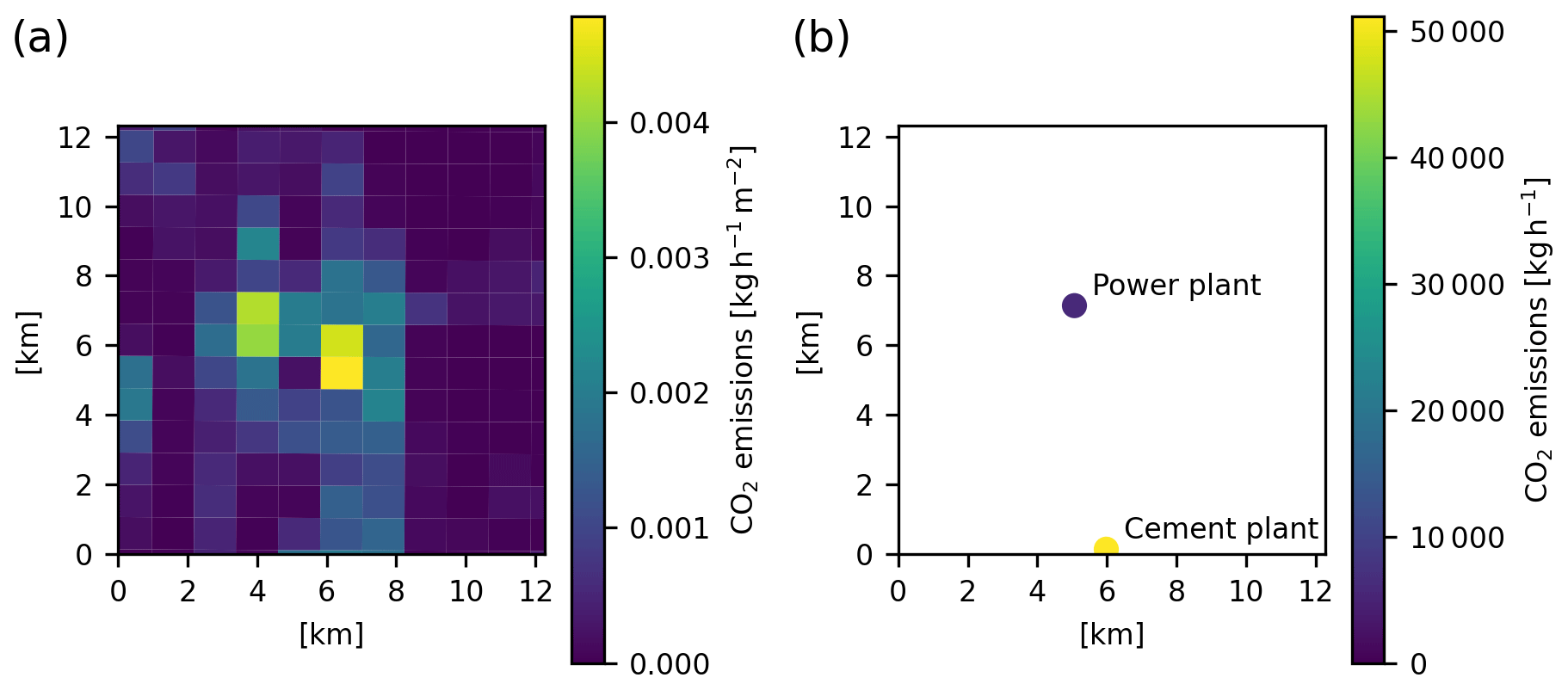
Figure B1(a) TNO area emissions, (b) TNO point emissions for the GRAL domain in Heidelberg. Data are taken from Super et al. (2020).
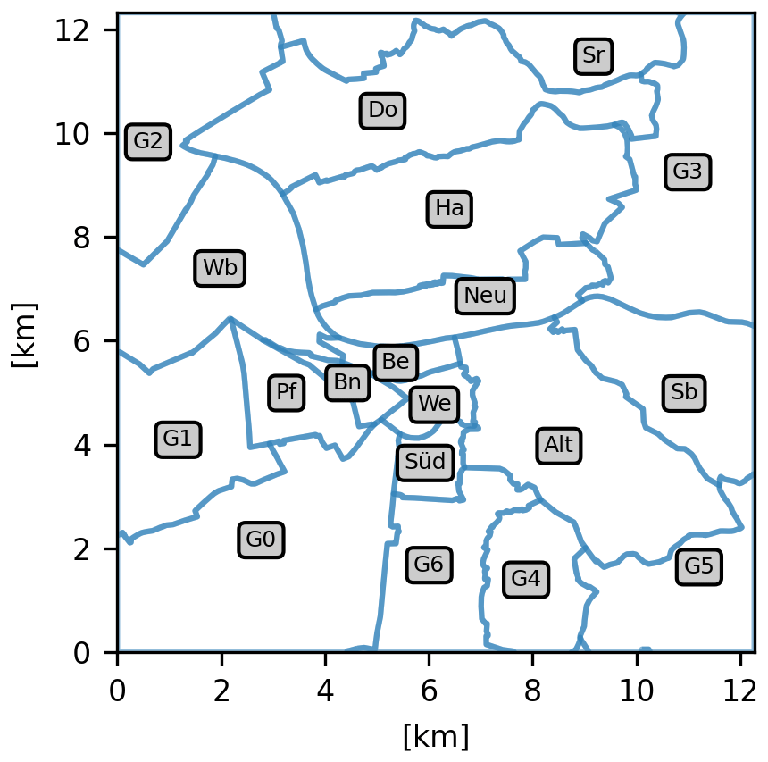
Figure C1The districts from OpenStreetMap used as states for the inversion. The full names as well as the administrative districts inside each district are listed in Table C1.
Table C1Overview of the district names and the administrative districts they represent. Smaller districts or district fragments are grouped together.
The inversion code can be found at https://doi.org/10.5281/zenodo.8354902 (Maiwald and Lüken-Winkels, 2023) and https://github.com/ATMO-IUP-UHEI/BayesInverse/tree/v.1.1 (last access: 26 February 2024). Code to read and process GRAMM/GRAL output: https://github.com/ATMO-IUP-UHEI/GGpyManager (last access: 23 February 2024) and https://doi.org/10.5281/zenodo.8375169 (Maiwald, 2023a). Code to conduct the experiments: https://github.com/ATMO-IUP-UHEI/Experiments (last access: 27 February 2024; DOI: https://doi.org/10.5281/zenodo.8370230, Maiwald, 2023b). Forward modelled concentration data has been simulated using GRAMM/GRAL v19.1 (https://github.com/GralDispersionModel, last access: 23 February 2024) and is archived on heiData: https://doi.org/10.11588/data/NHIVDO (Vardag and Maiwald, 2023). The position of the administrative districts are from OpenStreetMap (https://openstreetmap.org/copyright, last access: 10 August 2022).
SNV conceptualised the experiments, set up the simulations, supervised the work and wrote the original draft together with RM. RM carried out the formal analysis, performed the simulations and developed the software code.
The contact author has declared that neither of the authors has any competing interests.
Publisher’s note: Copernicus Publications remains neutral with regard to jurisdictional claims made in the text, published maps, institutional affiliations, or any other geographical representation in this paper. While Copernicus Publications makes every effort to include appropriate place names, the final responsibility lies with the authors.
We thank André Butz for valuable discussions on the experimental design and results. We thank Christopher Lueken-Winkels for helpful comments on the final draft. For the publication fee we acknowledge financial support by the Deutsche Forschungsgemeinschaft within the funding programme “Open Access Publikationskosten” as well as by Heidelberg University.
This research was partly funded by the German Research Foundation (DFG) within the Excellence Strategy ExU 5.2 as granted by the Heidelberg Center for the Environment.
This paper was edited by Yongze Song and reviewed by Gerrit H. de Rooij and one anonymous referee.
Balashov, N. V., Davis, K. J., Miles, N. L., Lauvaux, T., Richardson, S. J., Barkley, Z. R., and Bonin, T. A.: Background heterogeneity and other uncertainties in estimating urban methane flux: results from the Indianapolis Flux Experiment (INFLUX), Atmos. Chem. Phys., 20, 4545–4559, https://doi.org/10.5194/acp-20-4545-2020, 2020. a
Berchet, A., Zink, K., Muller, C., Oettl, D., Brunner, J., Emmenegger, L., and Brunner, D.: A cost-effective method for simulating city-wide air flow and pollutant dispersion at building resolving scale, Atmos. Environ., 158, 181–196, https://doi.org/10.1016/j.atmosenv.2017.03.030, 2017a. a, b
Berchet, A., Zink, K., Oettl, D., Brunner, J., Emmenegger, L., and Brunner, D.: Evaluation of high-resolution GRAMM–GRAL (v15.12/v14.8) NOx simulations over the city of Zürich, Switzerland, Geosci. Model Dev., 10, 3441–3459, https://doi.org/10.5194/gmd-10-3441-2017, 2017b. a, b
Blocken, B.: LES over RANS in building simulation for outdoor and indoor applications: A foregone conclusion?, Building Simulation, 11, 821–870, https://doi.org/10.1007/s12273-018-0459-3, 2018. a
Bréon, F. M., Broquet, G., Puygrenier, V., Chevallier, F., Xueref-Remy, I., Ramonet, M., Dieudonné, E., Lopez, M., Schmidt, M., Perrussel, O., and Ciais, P.: An attempt at estimating Paris area CO2 emissions from atmospheric concentration measurements, Atmos. Chem. Phys., 15, 1707–1724, https://doi.org/10.5194/acp-15-1707-2015, 2015. a
Davis, K. J., Deng, A., Lauvaux, T., Miles, N. L., Richardson, S. J., Sarmiento, D. P., Gurney, K. R., Hardesty, R. M., Bonin, T. A., Brewer, W. A., Lamb, B. K., Shepson, P. B., Harvey, R. M., Cambaliza, M. O., Sweeney, C., Turnbull, J. C., Whetstone, J., and Karion, A.: The Indianapolis Flux Experiment (INFLUX): A test-bed for developing urban greenhouse gas emission measurements, Elementa: Science of the Anthropocene, 5, 21, https://doi.org/10.1525/elementa.188, 2017. a
Delaria, E. R., Kim, J., Fitzmaurice, H. L., Newman, C., Wooldridge, P. J., Worthington, K., and Cohen, R. C.: The Berkeley Environmental Air-quality and CO2 Network: field calibrations of sensor temperature dependence and assessment of network scale CO2 accuracy, Atmos. Meas. Tech., 14, 5487–5500, https://doi.org/10.5194/amt-14-5487-2021, 2021. a, b
Deng, A., Lauvaux, T., Davis, K. J., Gaudet, B. J., Miles, N., Richardson, S. J., Wu, K., Sarmiento, D. P., Hardesty, R. M., Bonin, T. A., Brewer, W. A., and Gurney, K. R.: Toward reduced transport errors in a high resolution urban CO2 inversion system, Elementa: Science of the Anthropocene, 5, 20, https://doi.org/10.1525/elementa.133, 2017. a
Denier van der Gon, H. A. C., Hendriks, C., Kuenen, J., Segers, A., and Visschedijk, A. J. H.: Description of current temporal emission patterns and sensitivity of predicted AQ for temporal emission patterns, EU FP7 MACC deliverable report D_D-EMIS_1.3, https://atmosphere.copernicus.eu/sites/default/files/2019-07/MACC_TNO_del_1_3_v2.pdf (last access: 23.02.2023), 2011. a
Jungmann, M., Vardag, S. N., Kutzner, F., Keppler, F., Schmidt, M., Aeschbach, N., Gerhard, U., Zipf, A., Lautenbach, S., Siegmund, A., Goeschl, T., and Butz, A.: Zooming-in for climate action – hyperlocal greenhouse gas data for mitigation action?, Climate Action, 1, 8, https://doi.org/10.1007/s44168-022-00007-4, 2022. a, b
Kunik, L., Mallia, D. V., Gurney, K. R., Mendoza, D. L., Oda, T., and Lin, J. C.: Bayesian inverse estimation of urban CO2 emissions: Results from a synthetic data simulation over Salt Lake City, UT, Elementa: Science of the Anthropocene, 7, 36, https://doi.org/10.1525/ELEMENTA.375, 2019. a, b, c, d
Lauvaux, T., Miles, N. L., Richardson, S. J., Deng, A., Stauffer, D. R., Davis, K. J., Jacobson, G., Rella, C., Calonder, G.-P., and DeCola, P. L.: Urban Emissions of CO2 from Davos, Switzerland: The First Real-Time Monitoring System Using an Atmospheric Inversion Technique, J. Appl. Meteorol. Clim., 52, 2654–2668, https://doi.org/10.1175/JAMC-D-13-038.1, 2013. a
Lauvaux, T., Miles, N. L., Deng, A., Richardson, S. J., Cambaliza, M. O., Davis, K. J., Gaudet, B., Gurney, K. R., Huang, J., O'Keefe, D., Song, Y., Karion, A., Oda, T., Patarasuk, R., Razlivanov, I., Sarmiento, D., Shepson, P., Sweeney, C., Turnbull, J., and Wu, K.: High-resolution atmospheric inversion of urban CO2 emissions during the dormant season of the Indianapolis Flux Experiment (INFLUX), J. Geophys. Res.-Atmos., 121, 5213–5236, https://doi.org/10.1002/2015JD024473, 2016. a
Lian, J., Lauvaux, T., Utard, H., Bréon, F.-M., Broquet, G., Ramonet, M., Laurent, O., Albarus, I., Cucchi, K., and Ciais, P.: Assessing the Effectiveness of an Urban CO2 Monitoring Network over the Paris Region through the COVID-19 Lockdown Natural Experiment, Environ. Sci. Technol., 56, 2153–2162, https://doi.org/10.1021/ACS.EST.1C04973, 2022. a
Maiwald, R.: ATMO-IUP-UHEI/GGpyManager: First release of GGpyManager (v1.0), Zenodo [code], https://doi.org/10.5281/zenodo.8375169, 2023. a
Maiwald: ATMO-IUP-UHEI/Experiments: OSSE experiments with GRAMM-GRAL (v1.0.0), Zenodo [code], https://doi.org/10.5281/zenodo.8370230, 2023. a
Maiwald, R. and Lüken-Winkels, C.: ATMO-IUP-UHEI/BayesInverse: V.1.1 release of BayesInverse (v.1.1), Zenodo [code], https://doi.org/10.5281/zenodo.8354902, 2023. a
Mallia, D. V., Mitchell, L. E., Kunik, L., Fasoli, B., Bares, R., Gurney, K. R., Mendoza, D. L., and Lin, J. C.: Constraining Urban CO2 Emissions Using Mobile Observations from a Light Rail Public Transit Platform, Environ. Sci. Technol., 54, 15613–15621, https://doi.org/10.1021/acs.est.0c04388, 2020. a
Mano, Z., Kendler, S., and Fishbain, B.: Information Theory Solution Approach to the Air Pollution Sensor Location–Allocation Problem, Sensors, 22, 3808, https://doi.org/10.3390/s22103808, 2022. a
Miles, N. L., Davis, K. J., Richardson, S. J., Lauvaux, T., Martins, D. K., Deng, A. J., Balashov, N., Gurney, K. R., Liang, J., Roest, G., Wang, J. A., and Turnbull, J. C.: The influence of near-field fluxes on seasonal carbon dioxide enhancements: results from the Indianapolis Flux Experiment (INFLUX), Carbon Balance and Management, 16, 4, https://doi.org/10.1186/s13021-020-00166-z, 2021. a
Nathan, B. J., Lauvaux, T., Turnbull, J. C., Richardson, S. J., Miles, N. L., and Gurney, K. R.: Source Sector Attribution of CO2 Emissions Using an Urban Bayesian Inversion System, J. Geophys. Res.-Atmos., 123, 13611–13621, https://doi.org/10.1029/2018JD029231, 2018. a, b
Oda, T., Lauvaux, T., Lu, D., Rao, P., Miles, N. L., Richardson, S. J., and Gurney, K. R.: On the impact of granularity of space-based urban CO2 emissions in urban atmospheric inversions: A case study for Indianapolis, IN, Elementa: Science of the Anthropocene, 5, 28, https://doi.org/10.1525/elementa.146, 2017. a
Oettl, D.: Documentation of the prognostic mesoscale model GRAMM (Graz Mesoscale Model) Version 19.1, edited by: Goverment of Styria, Technical report, 1–125, 2019. a, b
Oettl, D.: Documentation of the Lagrangian Particle Model GRAL Vs. 19.01, edited by: Goverment of Styria, Technical report, 1–208, 2019. a
Richardson, S. J., Miles, N. L., Davis, K. J., Lauvaux, T., Martins, D. K., Turnbull, J. C., McKain, K., Sweeney, C., and Cambaliza, M. O. L.: Tower measurement network of in-situ CO2, CH4, and CO in support of the Indianapolis FLUX (INFLUX) Experiment, Elementa: Science of the Anthropocene, 5, 59, https://doi.org/10.1525/elementa.140, 2017. a
Rodgers, C. D.: Inverse methods for atmospheric sounding: Theory and practice, in: Series on Atmospheric, Oceanic and Planetary Physics, vol. 2, World Scientific Publishing, ISBN 981-02-2740-X, 2000. a, b, c, d
Super, I., Dellaert, S. N. C., Visschedijk, A. J. H., and Denier van der Gon, H. A. C.: Uncertainty analysis of a European high-resolution emission inventory of CO2 and CO to support inverse modelling and network design, Atmos. Chem. Phys., 20, 1795–1816, https://doi.org/10.5194/acp-20-1795-2020, 2020. a, b, c
Thompson, R. L. and Pisso, I.: A flexible algorithm for network design based on information theory, Atmos. Meas. Tech., 16, 235–246, https://doi.org/10.5194/amt-16-235-2023, 2023. a
Turnbull, J. C., Sweeney, C., Karion, A., Newberger, T., Lehman, S. J., Tans, P. P., Davis, K. J., Lauvaux, T., Miles, N. L., Richardson, S. J., Cambaliza, M. O., Shepson, P. B., Gurney, K., Patarasuk, R., and Razlivanov, I.: Toward quantification and source sector identification of fossil fuel CO2 emissions from an urban area: Results from the INFLUX experiment, J. Geophys. Res.-Atmos., 120, 292–312, https://doi.org/10.1002/2014JD022555, 2015. a
Turnbull, J. C., Karion, A., Davis, K. J., Lauvaux, T., Miles, N. L., Richardson, S. J., Sweeney, C., McKain, K., Lehman, S. J., Gurney, K. R., Patarasuk, R., Liang, J., Shepson, P. B., Heimburger, A., Harvey, R., and Whetstone, J.: Synthesis of Urban CO2 Emission Estimates from Multiple Methods from the Indianapolis Flux Project (INFLUX), Environ. Sci. Technol., 53, 287–295, https://doi.org/10.1021/acs.est.8b05552, 2019. a
Turner, A. J., Shusterman, A. A., McDonald, B. C., Teige, V., Harley, R. A., and Cohen, R. C.: Network design for quantifying urban CO2 emissions: assessing trade-offs between precision and network density, Atmos. Chem. Phys., 16, 13465–13475, https://doi.org/10.5194/acp-16-13465-2016, 2016. a, b, c, d, e
Ulrich, V., Brückner, J., Schultz, M., Vardag, S. N., Ludwig, C., Fürle, J., Zia, M., Lautenbach, S., and Zipf, A.: Private Vehicles Greenhouse Gas Emission Estimation at Street Level for Berlin Based on Open Data, ISPRS Int. J. Geo-Inf., 12, 138, https://doi.org/10.3390/ijgi12040138, 2023. a
Vardag, S. N. and Maiwald, Robert: Optimising Urban Measurement Networks for CO2 Flux Estimation: A High-Resolution Observing System Simulation Experiment using GRAMM/GRAL [data], V1, heiDATA [data set], https://doi.org/10.11588/data/NHIVDO, 2023. a
Vogel, F. R., Hammer, S., Steinhof, A., Kromer, B., and Levin, I.: Implication of weekly and diurnal 14C calibration on hourly estimates of CO-based fossil fuel CO2 ata moderately polluted site in southwestern Germany, Tellus B, 62, 512–520, https://doi.org/10.1111/j.1600-0889.2010.00477.x, 2010. a
World Bank: Cities and Climate Change: An Urgent Agenda. Urban development series, Urban Development Series Knowledge Papers, https://openknowledge.worldbank.org/handle/10986/17381 (last access: 23 February 2024), 2010. a
Wu, K., Lauvaux, T., Davis, K. J., Deng, A., Coto, I. L., Gurney, K. R., and Patarasuk, R.: Joint inverse estimation of fossil fuel and biogenic CO2 fluxes in an urban environment: An observing system simulation experiment to assess the impact of multiple uncertainties, Elementa: Science of the Anthropocene, 6, 17, https://doi.org/10.1525/elementa.138, 2018. a
Wu, L., Broquet, G., Ciais, P., Bellassen, V., Vogel, F., Chevallier, F., Xueref-Remy, I., and Wang, Y.: What would dense atmospheric observation networks bring to the quantification of city CO2 emissions?, Atmos. Chem. Phys., 16, 7743–7771, https://doi.org/10.5194/acp-16-7743-2016, 2016. a
- Abstract
- Introduction
- Methodology
- Results
- Discussion
- Conclusions
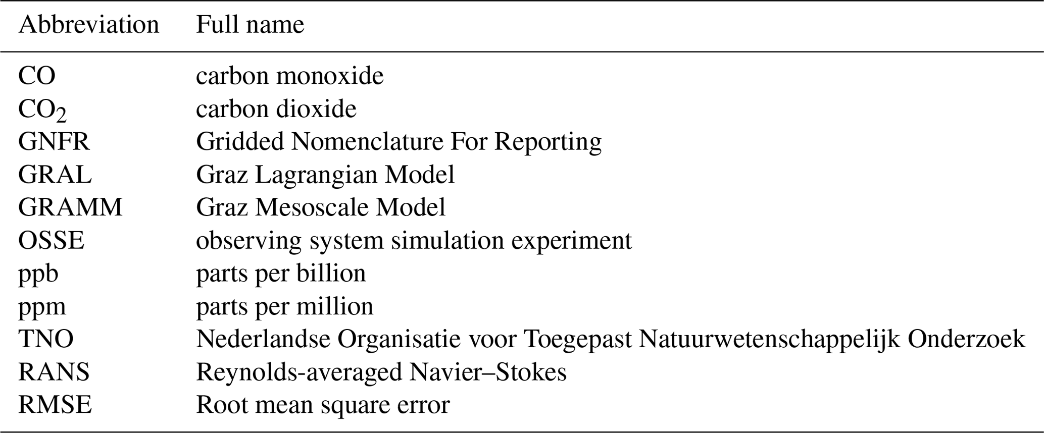
- Appendix A: Abbreviations
- Appendix B: Emissions
- Appendix C: Districts chosen as state vectors for the inversion
- Code and data availability
- Author contributions
- Competing interests
- Disclaimer
- Acknowledgements
- Financial support
- Review statement
- References
- Abstract
- Introduction
- Methodology
- Results
- Discussion
- Conclusions
- Appendix A: Abbreviations
- Appendix B: Emissions
- Appendix C: Districts chosen as state vectors for the inversion
- Code and data availability
- Author contributions
- Competing interests
- Disclaimer
- Acknowledgements
- Financial support
- Review statement
- References