New insights into the South China Sea throughflow and water budget seasonal cycle: evaluation and analysis of a high-resolution configuration of the ocean model SYMPHONIE version 2.4

The South China Sea throughflow (SCSTF) connects the South China Sea (SCS) with neighboring seas and oceans, transferring surface water of the global thermohaline circulation between the Pacific and Indian oceans. A configuration of the SYMPHONIE ocean model at high resolution (4 km) and including an explicit representation of tides is implemented over this region, and a simulation is analyzed over 2010–2018. Comparisons with in situ and satellite data and other available simulations at coarser resolution show the good performance of the model and the relevance of the high resolution for reproducing the spatial and temporal variability of the characteristics of surface dynamics and water masses over the SCS. The added value of an online computation of each term of the water, heat, and salt SCS budgets (surface, lateral oceanic and river fluxes, and internal variations) is also quantitatively demonstrated: important discards are obtained with offline computation, with relative biases of ∼40 % for lateral oceanic inflows and outflows.

The SCS water volume budget, including the SCSTF, is analyzed at climatological and seasonal scales. The SCS receives on average a 4.5 Sv yearly water volume input, mainly from the Luzon Strait. It laterally releases this water to neighboring seas, mainly to the Sulu Sea through Mindoro Strait (49 %), to the East China Sea via Taiwan Strait (28 %), and to the Java Sea through Karimata Strait (22 %). The seasonal variability of this water volume budget is driven by lateral interocean exchanges. Surface interocean exchanges, especially at Luzon Strait, are all driven by monsoon winds that favor winter southwestward flows and summer northeastward surface flows. Exchanges through Luzon Strait deep layers show a stable sandwiched structure with vertically alternating inflows and outflows. Last, differences in flux estimates induced by the use of a high-resolution model vs. a low-resolution model are quantified.

1 Introduction

The South China Sea (SCS, Fig. 1a), the largest marginal sea in the world, is subject to a wide range of forcings at different scales of both natural and anthropic origins. Its coasts are among the most densely populated regions in the world (CIESIN, 2018). The SCS is a source of subsistence for these populations (fishing, tourism, etc.) and is reciprocally affected by the harmful effects of human activities (pollution, resources overexploitation, etc.). The SCS plays an important role in regional and global ocean circulation and climate, transferring the surface water masses of the global thermohaline circulation between the Pacific and Indian oceans (Qu et al., 2005; Tozuka et al., 2007). It is therefore essential to understand, quantify, and monitor the respective contributions of the lateral oceanic, atmospheric, and continental fluxes in the SCS water, heat and salt budgets, and their interactions.

Ocean dynamics drive the transport and mixing of water masses and are thus strongly involved in the functioning and variability of the water, heat, and salt budgets of the SCS. They also determine the fate and functioning of matter in the marine compartment (planktonic ecosystems, contaminants, sediments). The SCS ocean circulation is regulated by a combination of factors, including the geometry of the zone, the tides, the connection with the western Pacific and eastern Indian oceans, and the atmospheric forcing from daily to seasonal and interannual scales (Wyrtki, 1961; Shaw and Chao, 1994; Metzger and Hurlburt, 1996; Gan et al., 2006). In the upper layer, the SCS basin-scale circulation is mainly driven by the seasonal monsoon winds (Liu et al., 2002; Liu and Gan, 2017). In winter, strong northeasterly monsoon winds generate a cyclonic circulation in the surface and upper layers over the whole basin. In summer, weaker southwesterly monsoon winds lead to a cyclonic gyre in the north and an anticyclonic gyre in the south (Qu, 2000; Gan et al., 2016). At the interannual timescale, the SCS circulation is impacted by the El Niño–Southern Oscillation (ENSO), via its effect on monsoon winds (Soden et al., 1999; Liu et al., 2014; Tan et al., 2016) but also via the direct propagation of ENSO oceanic signals from the western Pacific Ocean through the Luzon Strait (Qu et al., 2004; C. Wang et al., 2006). Other studies also suggested an impact of the Pacific Decadal Oscillation (PDO) on the SCS related to its effect on the intrusion of western Pacific water (Yu and Qu, 2013) and on the atmospheric water flux (Zeng et al., 2018). On the other side of the spectrum, the SCS is frequently crossed by tropical cyclones (Wang et al., 2007) that also affect ocean dynamics (Pan and Sun, 2013) and ecosystems (Liu et al., 2019). Last but not least, mesoscale to submesoscale structures play a significant role in the water mass dynamics and transports within the SCS (Liu et al., 2008; Chen et al., 2011; Nan et al., 2015; Da et al., 2019; Lin et al., 2020; Ni et al., 2021; Herrmann et al., 2023).

The SCS is connected with surrounding oceans and seas by several straits (Fig. 1a, white lines). The sills of the Luzon and Mindoro straits are 3000 and 400 m deep, respectively, while the other straits are less than 100 m deep. The Luzon Strait – the largest and deepest interocean strait of the zone – is the main pathway of seawater from the Pacific Ocean into the SCS (Wyrtki, 1961). Besides, the SCS exchanges seawater with the East China Sea through the Taiwan Strait, with the Sulu Sea through the straits of Balabac and Mindoro, and with the Java Sea and Andaman Sea (Indian Ocean) through Karimata and Malacca straits. The Mindoro, Balabac, and Malacca straits are particularly narrow, with their widest passages not being wider than 80, 55, and 20 km, respectively. Based on numerical studies, satellite observations and long-term wind data analyzes, Qu et al. (2005) and Yu et al. (2007) revealed a circulation where Pacific Ocean water masses enter the SCS through the Luzon Strait and leave the basin through the Taiwan, Karimata, and Mindoro straits, forming the South China Sea throughflow (SCSTF). Those lateral transports are involved in the SCS cycle of water, heat, and salt and interact with the atmospheric and continental components of this regional cycle. The SCS indeed receives net gains of freshwater and heat from the atmosphere and rivers. Estimates of net surface heat gain vary from 17 to 51 W m⁻² (Yang et al., 1999; Qu et al., 2004; Yu and Weller, 2007; Fang et al., 2009; Wang et al., 2019), and estimates of net water gain vary between 0.05 and 0.2 Sv (Qu et al., 2006; Fang et al., 2009).

Previous estimates of water volume, heat, and salt transports at the straits were performed based on in situ and satellite observations (Fang et al., 1991; Chu and Li, 2000; Chung et al., 2001; Wang et al., 2003; Tian et al., 2006; Yuan et al., 2008; Fang et al., 2010; Qu and Song, 2009; Sprintall et al., 2012; Susanto et al., 2013). However, in situ estimates remain limited in space and time and are made complicated by the complex topography in the region. Numerical modeling is a relevant tool to complement in situ and satellite measurements. Several modeling studies based on an integrated approach considering all terms of the budgets were performed, mainly focusing on water volume fluxes. Yaremchuk et al. (2009) provided estimates of upper water volume transport at the Luzon, Taiwan, Mindoro, and Karimata straits issued from a reduced-gravity model. Wang et al. (2009), using a ∼18 km resolution model, evaluated the seawater fluxes through all SCS interocean straits. In both studies, the inflow at Luzon was considered to be balanced by the outflows at other straits, i.e., internal variations were neglected, and the contribution from the atmosphere and rivers was not considered. Liu et al. (2011), Hsin et al. (2012), Tozuka et al. (2015), and Wei et al. (2016) provided estimates of the SCS interocean water volume transports with higher-resolution numerical models, but model configurations and assumptions did not allow us to rigorously close the water volume budget. Several studies addressed the question of heat and salt fluxes. Qu et al. (2004) studied the whole depth water volume transports through Luzon, Mindoro, and Sunda straits and the upper heat budget of the zone, revealing that the surface heat flux is the primary heating process. However, their numerical study was carried out with a closed Taiwan Strait and a shallower Mindoro Strait than reality, the inflow at Luzon was balanced by outflows at Mindoro and Sunda straits, and the river heat flux was neglected. Qu et al. (2006), using a ∼11 km resolution model, estimated the total water volume, heat, and freshwater SCSTF, deducing surface heat and freshwater transports from the difference between the inflowing and outflowing fluxes of temperature and salinity. Fang et al. (2005, 2009) were the first, followed by Wang et al. (2019), to evaluate transports through all interocean straits of the SCS, using ∼18 km then ∼7 km resolution models, respectively, but assuming that outflows compensate for inflows.

Those studies considerably improved our understanding of water volume, heat, and salt transport through the SCS area. However, they were associated with several limitations. First, they assumed that the SCS is at equilibrium over the studied periods, i.e., that the same amount of water volume, heat, and salt that enters the basin leaves it, and they used this assumption to deduce atmosphere and rivers contributions. Though this assumption allows us to close the budget at the first order, it does not account for possible internal variations and trends in the water volume, heat, and salt contents of the SCS. Yet Zeng et al. (2014, 2018), using in situ measurements and satellite data, evidenced a freshening of the SCS from 2010 to 2012 followed by a salinification until 2016, suggesting an interannual variability in salt and/or water mass content. Moreover, very few studies jointly examined the water volume, heat, and salt budgets, which is however necessary to provide consistent estimates of all the terms involved in those budgets and understand their interactions. Besides, using available (re)analysis to study those budgets requires us to compute them offline based on daily, weekly, or even monthly distributed outputs, thus neglecting the turbulent term of temperature and salinity lateral transports. The error associated with this assumption are required to be assessed. Last, the model's resolution was rarely finer than 10 km, and they did not represent tides. As pointed out by Lin et al. (2020), models at higher resolution and including tides are necessary to represent the full range of temporal and spatial scales involved in the transport and mixing of water masses through the SCS. This includes the mesoscale to submesoscale eddies and structures of size smaller than 40 km (Da et al., 2019; Ni et al., 2021; Herrmann et al., 2023), as well as the detailed topography and dynamics of coastal areas and key straits, some of which are less than 20 km wide, where interocean exchanges and strong internal tidal mixing occur (e.g., at Luzon Strait but also at narrow straits like Malacca, Mindoro, and Balabac, Hatayama et al., 1996; Laurent, 2008; Wang et al., 2016). Xu et al. (2022) indeed showed for the Atlantic Ocean that using in a model combining a high-resolution ($\mathrm{1}/\mathrm{50}\mathit{°}$) bathymetry and explicit tides improved the representation of internal waves and consequently of the mesoscale sea surface height wavenumber spectrum over the tropical ocean. Sannino et al. (2009) and Chassignet et al. (2023) moreover pointed out the relevance of high-resolution bathymetry for the representation of interocean strait exchanges and mesoscale activity involved in western boundary currents, respectively.

Following this introduction, our first scientific objective is to better understand the role of the SCS in the global circulation and regional climate at different scales, i.e., daily, seasonal, and interannual variability, by providing updated and consistent estimates at those scales of all the terms involved in the SCS water volume, heat, and salt budgets: lateral oceanic, atmospheric, and river fluxes and internal variations. For that, we developed a configuration of a regional ocean hydrodynamical model with a high spatial resolution (4 km) over the SCS and an explicit representation of tides, in order to represent as realistically as possible the wide range of scales and processes involved in the SCS dynamics and to study their contribution to SCS budgets. The water volume, heat, and salt budgets have been rigorously closed by performing online calculations of each term of those budgets, including incoming and outgoing flows. The first objective of this paper is to present and evaluate in detail this modeling tool, which will be used to study water volume, salt, and heat budgets and will be available to the community interested in addressing scientific questions related to SCS ocean dynamics functioning, variability, and influence. The second objective is to perform a first analysis at the climatological and seasonal scales of the water budget over the SCS and of its components, i.e.m river, atmospheric, and oceanic lateral fluxes and internal variations.

The paper is organized as follows. Section 2 presents the hydrodynamical model, its high-resolution configuration over the SCS and the observation data, and the other numerical simulations at coarser resolution used for its evaluation. The online computations of each term of the budgets are then detailed. The added value of the online computation compared to the offline computation is demonstrated in Sect. 3. The ability of the model to simulate the SCS sea surface dynamics and water mass characteristics at different scales is evaluated in Sect. 4 through comparisons with available in situ and satellite observations and with other simulations. An evaluation and an analysis of the water budget and its various components over the SCS are carried out on a climatological scale in Sect. 5, and lateral exchanges at interocean straits, corresponding to the SCSTF, are examined in detail. Results are summarized in Sect. 6, and an overview on the future applications of this high-resolution closed-budget modeling tool is provided.

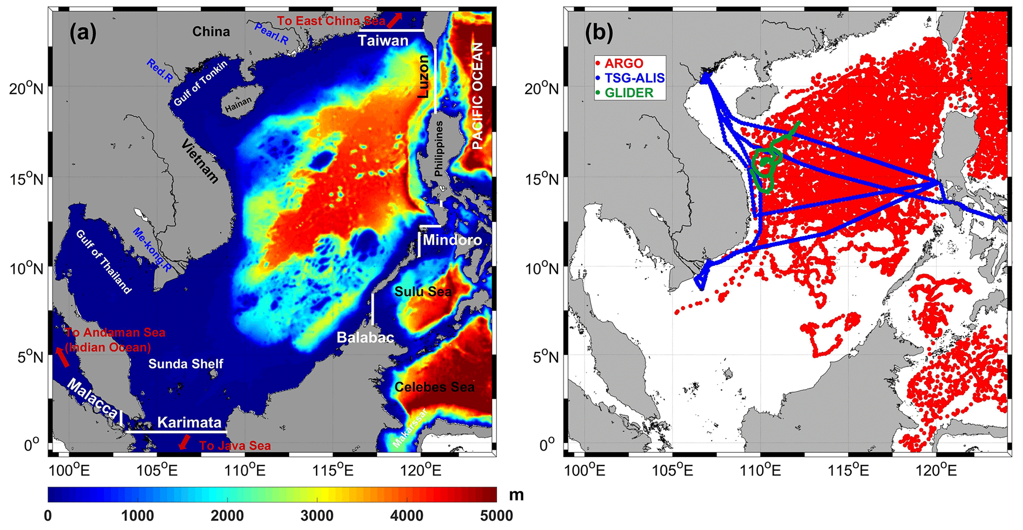
Figure 1 (a) Computational domain bathymetry (m) and interocean straits (white lines). (b) Maps of Argo float trajectories in the SCS from January 2009 to December 2018 (red), TSG from R/V Alis trajectory from May to July 2014 (blue), and glider trajectory from January to May 2017 (green).

2 Materials and methods

2.1 The numerical model SYMPHONIE

2.1.1 General presentation of the model

The 3-D ocean circulation model SYMPHONIE Marsaleix et al. (2008, 2019) is based on the Navier–Stokes primitive equations solved on an Arakawa curvilinear C-grid under the hydrostatic and Boussinesq approximations. The model makes use of an energy-conserving finite-difference method (Marsaleix et al., 2008), a forward–backward time-stepping scheme, a Jacobian pressure gradient scheme (Marsaleix et al., 2009), the equation of state of Jackett et al. (2006), and the K-epsilon turbulence scheme with the implementation described in Costa et al. (2017). Horizontal advection and diffusion of tracers are computed using the QUICKEST scheme (Leonard, 1979), and vertical advection is computed using a centered scheme. Horizontal advection and diffusion of momentum are each computed with a fourth-order centered biharmonic scheme. The biharmonic viscosity of momentum is calculated according to a Smagorinsky-like formulation derived from Griffies and Hallberg (2000). The lateral open boundary conditions, based on radiation conditions combined with nudging conditions, are described in Marsaleix et al. (2006) and boundary conditions at river mouths are described in Nguyen-Duy et al. (2021). As in Estournel et al. (2021), To Duy et al. (2022), and Hermann et al. (2023), the VQS (vanishing quasi-sigma) vertical coordinate is used, allowing us to avoid an excess of vertical levels in very shallow areas while maintaining an accurate description of the bathymetry and reducing the truncation errors associated with the sigma coordinate.

2.1.2 Model setup

The SYMPHONIE numerical configuration covers the whole SCS (0.6° S–24° N, 99–124° E, Fig. 1a), with a regular grid of 4 km horizontal resolution and 50 vertical levels in the deepest area. It is built from a bathymetry product merging GEBCO 2014 gridded bathymetry and digitalized nautical charts (Piton et al., 2020). Bathymetry ranges from 3 to 5000 m in the studied area (Fig. 1a). The simulation runs from 1 January 2009 to 31 December 2018 and is referred to as SYM4 in the following.

Initial and lateral oceanic boundary conditions for temperature, salinity, currents, and sea level are provided by the daily outputs of the Global_Analysis_Forecast_Phy_001_024 Global Ocean $\mathrm{1}/\mathrm{12}\mathit{°}$ physics analysis and forecast provided by Copernicus Marine Environment Monitoring Service (CMEMS) (http://marine.copernicus.eu; last access: 18 May 2023). The SYM4 simulation departs from an initial state that is not at rest since it includes the currents from CMEMS $\mathrm{1}/\mathrm{12}\mathit{°}$ analysis. The spin-up time, whose main aim is to energetically adjust the initial physical fields provided by CMEMS to the specific constraints of the SYM4 grid, lasts a few months. We therefore analyze the simulation over the period 1 January 2010–31 December 2018.

The SCS configuration includes 63 river mouths. Daily data were provided by the National Hydro-Meteorological Service of Vietnam for 11 rivers flowing in northern and central Vietnam (including the Red River). Monthly climatology runoff issued from the CLS–INDESO project were provided for the other rivers, including the Mekong and Pearl rivers (Tranchant et al., 2016).

The atmospheric forcing is calculated from the bulk formulae of Large and Yeager (2004) using the European Centre for Medium-Range Weather Forecasts (ECMWF) operational forecasts at $\mathrm{1}/\mathrm{8}\mathit{°}$ horizontal resolution and 3 h temporal resolution, available at https://www.ecmwf.int/, last access: 18 May 2023.

Open boundary tidal conditions are prescribed from FES2014b, the 2015 release of the FES (Finite Element Solution) global tide model (Carrere et al., 2016; Lyard et al., 2021) that assimilates altimetry satellite observations and tide gauge data. The data are freely available on the Aviso website: https://www.aviso.altimetry.fr/en/data/products/auxiliary-products/global-tide-fes.html (last access: 18 May 2023). The SCS configuration takes into account nine barotropic tidal components (in phase and altitude): M2, S2, N2, K2 (semi-diurnal tides), K1, P1, O1, Q1 (diurnal tides), and M4 (compound tide). The model is also forced by the astronomical plus the loading and self-attraction potentials (Lyard et al., 2006). Details and numerical issues related to tides can be found in Pairaud et al. (2008, 2010).

2.2 Flux calculation methods

We detail here the computation of each term of the water volume, heat, and salt budgets over the whole SCS: internal content variations and surface, oceanic lateral, and river fluxes. We compute lateral oceanic fluxes through the six interocean straits connecting the SCS to neighboring seas and oceans shown in Fig. 1a: Taiwan, Luzon, Mindoro, Balabac, Karimata, and Malacca straits. All the terms of the budget equations are computed online. The added value of the online computation compared to the offline computation is presented in Sect. 3.

2.2.1 Water volume, heat, and salt budget equations

Water volume, heat, and salt contents are rigorously conserved in SYMPHONIE, as shown below in Sect. 3 and Fig. 2: during each time step the variation (delta) of water volume, heat, or salt content in the numerical ocean domain is equal to the net input from sources and sinks, i.e., the sum of fluxes from rivers, the atmosphere, and lateral oceanic boundaries.

Water volume budget

The internal variation of water volume V over the SCS area between times t₁ and t₂ (ΔV) is equal to the integral between t₁ and t₂ of all water volume fluxes exchanged at the boundaries (atmosphere, rivers and lateral open ocean boundaries) of the SCS domain, taken as the sea zone limited by the six interocean straits shown in Fig. 1a:

$$\begin{array}{}\text{(1)}& \mathrm{\Delta }V=V_{t\mathrm{2}}-V_{t\mathrm{1}}=\underset{t_{\mathrm{1}}}{\overset{t_{\mathrm{2}}}{\int }}\left(F_{\mathrm{w},\mathrm{lat}}+F_{\mathrm{w},\mathrm{surf}}+F_{\mathrm{w},\mathrm{riv}}\right)\mathrm{d}t,\end{array}$$

where F_w,lat, F_w,surf, and F_w,riv are the net oceanic lateral, atmospheric surface, and river water volume fluxes, respectively. Here and in the following, positive fluxes correspond to inflows and negative fluxes to outflows.

Heat budget

The variation of heat content HC between times t₁ and t₂ (Δ HC) is equal to the sum of all heat fluxes exchanged at the boundaries of the SCS domain between t₁ and t₂:

$$\begin{array}{}\text{(2)}& \mathrm{\Delta }\mathrm{HC}={\mathrm{HC}}_{t\mathrm{2}}-{\mathrm{HC}}_{t\mathrm{1}}=\underset{t_{\mathrm{1}}}{\overset{t_{\mathrm{2}}}{\int }}\left(F_{T,\mathrm{lat}}+F_{T,\mathrm{surf}}+F_{T,\mathrm{riv}}\right)\mathrm{d}t,\end{array}$$

where F_T,lat, F_T,surf, and F_T,riv are the net oceanic lateral, atmospheric surface, and river heat fluxes, respectively, and HC is computed from

$$\begin{array}{}\text{(3)}& \mathrm{HC}={\mathit{\rho }}_{\mathrm{0}}{C}_p\underset{x}{\int }\underset{y}{\int }\underset{z}{\int }T\left(x,y,z,t\right)\mathrm{d}x\mathrm{d}y\mathrm{d}z,\end{array}$$

with T the temperature (in °C), ρ₀ the seawater density constant (1028 kg m⁻³), and C_p the seawater specific heat constant (3900 J kg⁻¹ °C⁻¹).

Salt budget

The salinity of water going to or coming from to the atmosphere and the rivers is assumed to be zero, meaning that there is no input or output of salt from surface atmospheric fluxes and river runoff. It should be noted that evaporation, precipitation, and river discharge are not sources or sinks of salt but are instead sources or sinks of salinity for the ocean domain: although they do not affect the salt budget of the ocean domain, atmospheric and river fluxes do modify the salinity budget, as they affect the water volume budget. The variation of salt content between t₁ and t₂ (ΔSC) is thus equal to the sum of salt fluxes exchanged at the lateral oceanic boundaries of the SCS domain:

$$\begin{array}{}\text{(4)}& \mathrm{\Delta }\mathrm{SC}={\mathrm{SC}}_{t\mathrm{2}}-{\mathrm{SC}}_{t\mathrm{1}}=\underset{t_{\mathrm{1}}}{\overset{t_{\mathrm{2}}}{\int }}{F}_{\mathrm{S},\mathrm{lat}}\mathrm{d}t,\end{array}$$

where F_S,lat is the net salt flux at the lateral oceanic boundaries and SC is computed from

$$\begin{array}{}\text{(5)}& \mathrm{SC}={\mathit{\rho }}_{\mathrm{0}}\underset{x}{\int }\underset{y}{\int }\underset{z}{\int }S(x,y,z,t)\mathrm{d}x\mathrm{d}y\mathrm{d}z,\end{array}$$

with S being the salinity.

2.2.2 Lateral fluxes through ocean open boundaries

The total lateral water volume flux F_w,lat through the vertical section A of an open-ocean boundary is computed in Sv (1 Sv =10⁶ m³ s⁻¹) from

$$\begin{array}{}\text{(6)}& F_{\mathrm{w},\mathrm{lat}}=\underset{A}{\int }{v}_{\mathrm{t}}\mathrm{d}A,\end{array}$$

with v_t the current velocity normal to the transect and A the area of the section from the surface to bottom.

The lateral heat flux F_T,lat in PW (PW =10¹⁵ W) is computed from

$$\begin{array}{}\text{(7)}& F_{T,\mathrm{lat}}={\mathit{\rho }}_{\mathrm{0}}{C}_p\underset{A}{\int }T{v}_t\mathrm{d}A.\end{array}$$

The lateral salt flux F_S,lat in Gg s⁻¹ is computed from

$$\begin{array}{}\text{(8)}& F_{\mathrm{S},\mathrm{lat}}={\mathit{\rho }}_{\mathrm{0}}\underset{A}{\int }{\mathrm{Sv}}_t\mathrm{d}A.\end{array}$$

Inflowing and outflowing fluxes are also computed using the same equations but for values of v_t>0 and v_t<0, respectively.

$$\begin{array}{c}{\displaystyle }\begin{array}{rl}{F}_{\mathrm{w},\mathrm{lat}+}& =\underset{A}{\int }{v}_{\mathrm{t}}/(v_{\mathrm{t}}>\mathrm{0})\mathrm{d}A\\ & \text{and}{F}_{\mathrm{w},\mathrm{lat}-}=\underset{A}{\int }{v}_{\mathrm{t}}/(v_{\mathrm{t}}<\mathrm{0})\mathrm{d}A(\mathrm{Eq}.{\mathrm{6}}^{\prime })\end{array}\\ {\displaystyle }\begin{array}{rl}{F}_{T,\mathrm{lat}+}& ={\mathit{\rho }}_{\mathrm{0}}{C}_p\underset{A}{\int }T{v}_t/(v_{\mathrm{t}}>\mathrm{0})\mathrm{d}A\\ & \text{and}{F}_{T,\mathrm{lat}-}={\mathit{\rho }}_{\mathrm{0}}{C}_p\underset{A}{\int }T{v}_t/(v_{\mathrm{t}}<\mathrm{0})\mathrm{d}A(\mathrm{Eq}.{\mathrm{7}}^{\prime })\end{array}\\ {\displaystyle }\begin{array}{rl}{F}_{\mathrm{S},\mathrm{lat}+}& ={\mathit{\rho }}_{\mathrm{0}}\underset{A}{\int }{\mathrm{Sv}}_t/(v_{\mathrm{t}}>\mathrm{0})\mathrm{d}A\\ & \text{and}{F}_{\mathrm{S},\mathrm{lat}-}={\mathit{\rho }}_{\mathrm{0}}\underset{A}{\int }{\mathrm{Sv}}_t/(v_{\mathrm{t}}<\mathrm{0})\mathrm{d}A(\mathrm{Eq}.{\mathrm{8}}^{\prime })\end{array}\end{array}$$

2.2.3 River fluxes

The river water volume flux F_w,riv is calculated as the sum over all the rivers of the product of the velocity of river flow at the river mouth, v_riv:

$$\begin{array}{}\text{(9)}& F_{\mathrm{w},\mathrm{riv}}={\sum }_{\mathrm{rivers}}\underset{A}{\int }{v}_{\mathrm{riv}}\mathrm{d}A,\end{array}$$

where A is the area of the river mouth section from the surface to the bottom.

The river heat flux F_T,riv in PW is computed from

$$\begin{array}{}\text{(10)}& F_{T,\mathrm{riv}}={\sum }_{\mathrm{rivers}}{\mathit{\rho }}_{\mathrm{0}}{C}_p\underset{A}{\int }T{v}_{\mathrm{riv}}\mathrm{d}A,\end{array}$$

where T is the temperature (in °C) at the river mouth.

2.2.4 Atmospheric (surface) fluxes

The atmospheric freshwater volume flux is computed in Sv (1 Sv =10⁶ m³ s⁻¹) from

$$\begin{array}{}\text{(11)}& F_{\mathrm{w},\mathrm{surf}}=\underset{\mathrm{Surf}}{\int }(P-E)\mathrm{d}x\mathrm{d}y,\end{array}$$

where P stands for the precipitation in m s⁻¹, E the evaporation in m s⁻¹, and Surf is the SCS area limited by the six interocean straits shown in Fig. 1a.

The net surface heat flux (F_T,surf) in PW is the sum over the SCS of the short-wave radiation flux (F_SR), long-wave radiation flux (F_LR), sensible heat flux (F_SEN), and latent heat flux (F_LATENT):

$$\begin{array}{}\text{(12)}& F_{T,\mathrm{surf}}=\underset{\mathrm{Surf}}{\int }(F_{\mathrm{SR}}+F_{\mathrm{LR}}+F_{\mathrm{SEN}}+F_{\mathrm{LATENT}})\mathrm{d}x\mathrm{d}y.\end{array}$$

Finally, it should be noted that the flux calculations are numerically consistent with those carried out by the model through the advection scheme and its surface and continental boundary conditions. Along these lines, C_p and ρ₀ constants correspond to the values used by the bulk formulas and the horizontal fluxes are calculated in the same way as in the advection scheme of the model. This allows us to produce a strictly closed budget: the sum of all fluxes explains 100 % of the variations of the water volume and of the total heat and salt contents at each time step of the simulation, as will be shown in Sect. 3.

2.3 Observational datasets

Satellite and tide gauge data are used for evaluating the representation of ocean surface characteristics (temperature, salinity, elevation). In situ data are used to evaluate the surface and vertical representation of water mass properties and the mixed-layer depth (MLD).

2.3.1 Satellite data

To evaluate the modeled SST (sea surface temperature), we use daily OSTIA (Operational Sea Surface Temperature and Sea Ice Analysis) outputs for the period 2010–2018, available at https://data.nodc.noaa.gov/ghrsst/L4/GLOB/UKMO/OSTIA/ (last access: 18 May 2023). OSTIA is a GHRSST (Group for High Resolution Sea Surface Temperature) Level 4 SST daily product built from multiple spatial sensors and drifting and moored buoys data, with a horizontal resolution of $\mathrm{1}/\mathrm{18}\mathit{°}$.

Regarding the SSS (sea surface salinity), we use outputs from the 9 d averaged de-biased SMOS (Soil Moisture and Ocean Salinity) SSS Level 3 version 3, developed by Boutin et al. (2016). It has a resolution of 25 km and is available for the period 2010–2017. Data are distributed by the CECOS (Ocean Salinity Expertise Center) and the CNES–IFREMER CATDS (Centre Aval de Traitement des Données SMOS) via https://data.catds.fr/cecos-locean/Ocean_products/L3_DEBIAS_LOCEAN/ (last access: 18 May 2023).

To evaluate the SLA (sea level anomaly) and surface geostrophic currents, we use daily $\mathrm{1}/\mathrm{4}\mathit{°}$ global ocean gridded L4 sea surface heights in the delayed–time of CMEMS dataset, available at https://data.marine.copernicus.eu/product/SEALEVEL_GLO_PHY_L4_MY_008_047/description (last access: 18 May 2023). This altimetry product (hereafter called ALTI) is generated using data from different altimeter missions and covers the period from 1993 up to present (Ablain et al., 2015; Ray and Zaron, 2016). For model–data comparison, we extracted the daily altimetric SLA on the period of comparison and removed at each point of each dataset (model and altimetry) the temporal average over the same period.

2.3.2 In situ data

More than 12 000 Argo profiles were collected in the SCS between 2010 and 2018 (see Fig. 1b), available from https://data-argo.ifremer.fr/geo/pacific_ocean/ (last access: 18 May 2023, https://doi.org/10.17882/42182).

The R/V ALIS crossed the SCS from 10 May to 28 July 2014 (see Fig. 1b), measuring SST and SSS every 6 s using a vessel-mounted Seabird SBE21 thermosalinometer (hereafter called TSG-Alis data).

Under the framework of a cooperative Vietnam–US international research program (Rogowski et al., 2019), a Seaglider sg206 was deployed on 22 January until 16 May 2017 in the SCS (see Fig. 1b). It collected 555 vertical profiles of conductivity, temperature, and pressure from an unpumped Sea-Bird Electronics CTD (conductivity, temperature, and depth) device (SBE 41CP). Conductivity, temperature, and depth were sampled at 5 s intervals in the upper 150 m, corresponding to a resolution finer than 1 m, and between 55 and 100 s below. All sensors were factory calibrated. Salinity was corrected for the thermal lag error using a variable flow rate (Garau et al., 2011).

Argo, TS-Alis, and glider in situ measurements are compared in Sect. 4 with modeled profiles at the nearest point (in position and time).

The third version of GESLA (Global Extreme Sea Level Analysis) dataset, released in 2021, consists of 5119 tidal records obtained from multiple sources around the world (Haigh et al., 2023). This quasi-global, higher-frequency tide gauges dataset can be obtained from https://www.gesla.org (last access: 5 September 2023). Tide gauge records from 46 stations are collected over the SCS region, then compared with modeled tidal outputs at the nearest point.

2.4 Other global and regional models

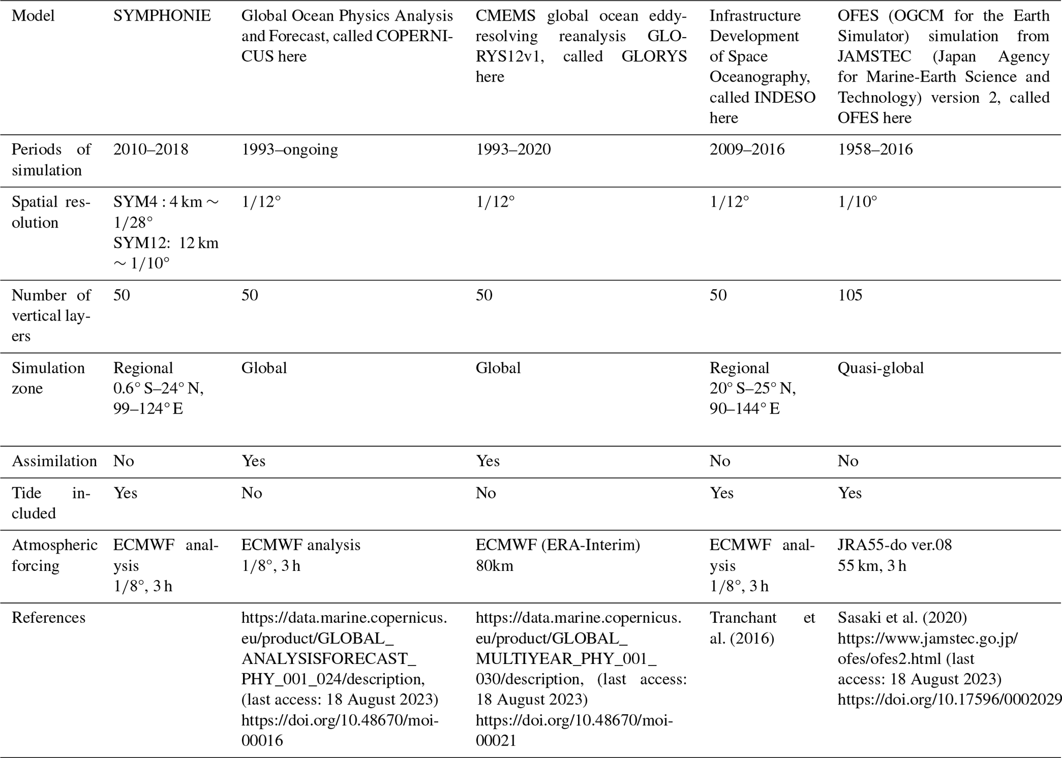
Besides the observational dataset, four widely used model outputs (COPERNICUS, INDESO, OFES, and GLORYS; see Table 1) are collected and compared with our SYM4 simulation over the same geographic zone (0.6–24° N, 99–124° E) from 2010 to 2016, the common simulation period of all models. In addition, a SYMPHONIE simulation using exactly the same configuration as SYM4 but with a coarser horizontal resolution (12 km $\sim \mathrm{1}/\mathrm{10}\mathit{°}$), referred to as SYM12 in the following, is performed over the same period to study the influence of horizontal resolution on the model performance.

Table 1 Global and regional models used for the comparison with SYMPHONIE outputs.

2.5 Statistical evaluation

The simulated dataset S and observational dataset O (of the same size N) are compared using three statistical parameters: the bias, the normalized root-mean-square error (NRMSE), and the Pearson correlation coefficient R:

$$\begin{array}{}\text{(13)}& {\displaystyle }\mathrm{Bias}=\stackrel{\mathrm{‾}}{S}-\stackrel{\mathrm{‾}}{O}\text{(14)}& {\displaystyle }\mathrm{NRMSE}={\displaystyle \frac{\sqrt{\frac{\mathrm{1}}{N}{\sum }_{i=\mathrm{1}}^n(S_i-O_i{)}^{\mathrm{2}}}}{(O_{\max }-O_{\min })}}\text{(15)}& {\displaystyle }R={\displaystyle \frac{{\sum }_{i=\mathrm{1}}^N\left(O_i-\stackrel{\mathrm{‾}}{O}\right)\left(S_i-\stackrel{\mathrm{‾}}{S}\right)}{{\sum }_{i=\mathrm{1}}^N{\left(O_i-\stackrel{\mathrm{‾}}{O}\right)}^{\mathrm{2}}{\sum }_{i=\mathrm{1}}^N{\left(S_i-\stackrel{\mathrm{‾}}{S}\right)}^{\mathrm{2}}}}\end{array}$$

where S_i and O_i are the simulated and observed series, respectively, and $\stackrel{\mathrm{‾}}{S}$ and $\stackrel{\mathrm{‾}}{O}$ are their mean values. In Sect. 3, we use the same statistical evaluation methods for the comparison between online and offline computation of lateral oceanic fluxes: S_i, O_i, $\stackrel{\mathrm{‾}}{S}$, and $\stackrel{\mathrm{‾}}{O}$ are, respectively, replaced by OF_i (the offline fluxes series), ON_i (the online fluxes series), $\stackrel{\mathrm{‾}}{\mathrm{OF}}$, and $\stackrel{\mathrm{‾}}{\mathrm{ON}}$ (the corresponding mean values).

3 Added value of the online budget computation

Computing all the terms of the budget online allows us to calculate the exact net lateral fluxes through each lateral ocean boundary, and hence to rigorously close the budgets at all timescales but also to calculate the exact outflowing and inflowing fluxes at each time step. Computing the lateral term offline using the modeled velocity, temperature, and salinity at the output frequency, indeed relies on the assumption that the integral over the output period of the product of velocity and temperature (or salinity) is equal to the product of their integrals, and thus that the turbulent term $\stackrel{\mathrm{‾}}{u^{\prime }{T}^{\prime }}$ in the following equation is negligible:

$$\begin{array}{}\text{(16)}& \begin{array}{rl}\stackrel{\mathrm{‾}}{uT}& =\stackrel{\mathrm{‾}}{(\stackrel{\mathrm{‾}}{u}+u^{\prime })(\stackrel{\mathrm{‾}}{T}+T^{\prime })}=\stackrel{\mathrm{‾}}{\stackrel{\mathrm{‾}}{u}\stackrel{\mathrm{‾}}{T}}+\stackrel{\mathrm{‾}}{u^{\prime }\stackrel{\mathrm{‾}}{T}}+\stackrel{\mathrm{‾}}{T^{\prime }\stackrel{\mathrm{‾}}{u}}+\stackrel{\mathrm{‾}}{u^{\prime }{T}^{\prime }}\\ & =\stackrel{\mathrm{‾}}{u}\stackrel{\mathrm{‾}}{T}+\stackrel{\mathrm{‾}}{u{}^{\prime }T{}^{\prime }},\end{array}\end{array}$$

where u is the velocity normal to the vertical section, T the temperature at this point, and the overbar stands for the integral over the output period.

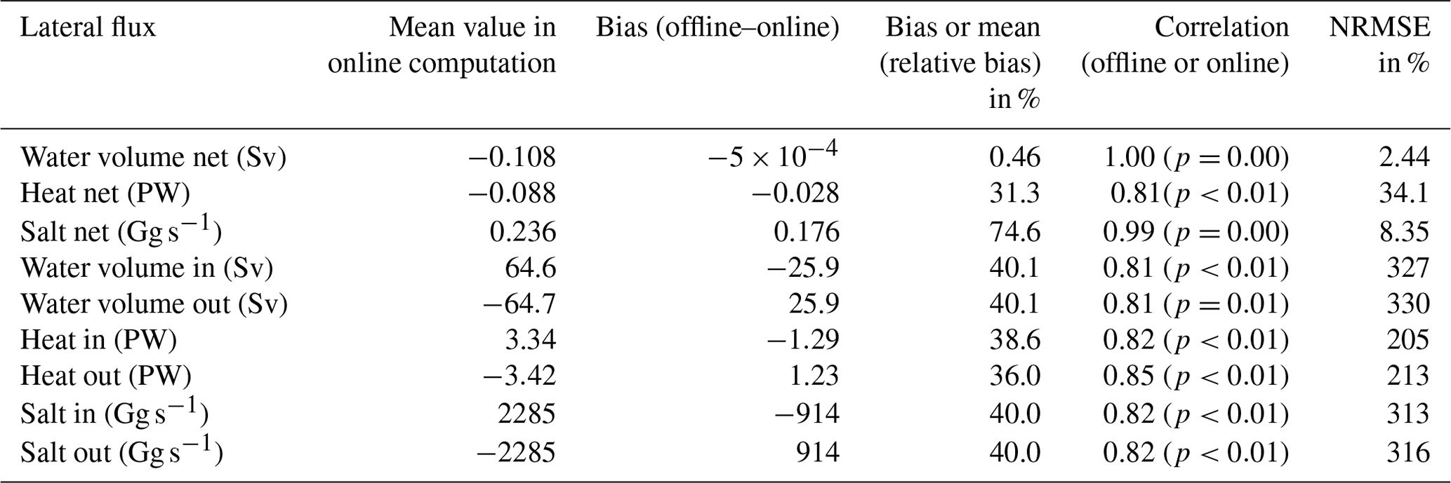
Here we quantitatively show the added value of the online computation of water volume, heat and salt budgets compared to the offline computation. In Fig. 2a, b, c we show each term of the budget equation for the interannual variations of water volume, heat, and salt contents over the SCS, computed online in SYM4 and offline from SYM4 outputs, i.e., annual variation, atmospheric surface fluxes, river fluxes, lateral oceanic fluxes, and the sum of all fluxes, that should equal the annual variation as explained in Sect. 2.2. Table 2 provides the values of net, inflowing, and outflowing annual fluxes computed online and the bias, correlation, and NRMSE between the offline and online computations.

First, those figures confirm that when computed online, the sum of annual fluxes is equal to the annual variation, i.e., that the budget equation is closed in our model. This is shown here for the interannual variations but is also verified at each time step of the whole simulation (figure not shown). Second, Fig. 2a, b, c quantitatively highlight the error induced when neglecting the turbulent term in Eq. (16) by computing the lateral net fluxes offline. For the water volume flux, using the online (blue) and offline (cyan) computation for net lateral oceanic fluxes is equivalent since it does not imply any nonlinear assumption. For the heat and salt fluxes however the difference is significant: we obtain NRMSEs of 34 % and 8 %, respectively, between the online and offline computations for heat and salt net lateral fluxes over the SCS for the 2010–2018 period (Table 2), respectively.

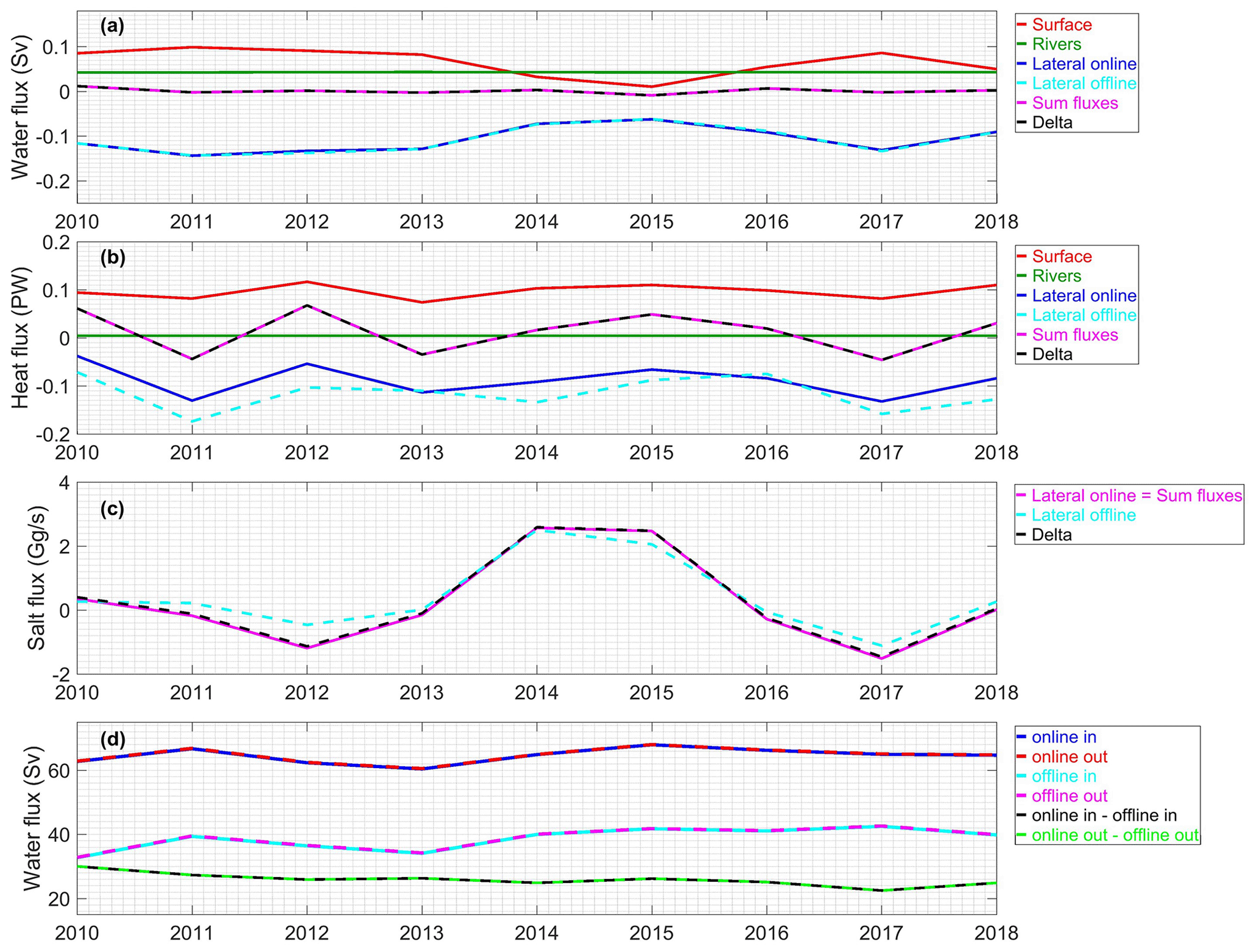
Figure 2 Atmospheric (surface, red), river (green), and net lateral oceanic (blue online, cyan offline) annual fluxes of (a) water volume (Sv), (b) heat (PW), and (c) salt (Gg s⁻¹); their sum (magenta); and annual variations of water volume, heat, and salt contents (black) over the period 2010–2018. (d) Annual lateral oceanic inflow (blue online, cyan offline) and outflow (red online, magenta offline) of water volumes (in absolute values) computed online and offline, and the difference between online and offline (black for inflow, green for outflow).

Third, the online computation allows us to separately compute the outflowing and inflowing terms of the lateral flux at each time step. Figure 2d shows the annual water volume lateral inflowing and outflowing fluxes (in absolute values) computed online and offline. Using the offline computational methods leads to important errors: the offline computation underestimates the water volume outflow and inflow by a factor of ∼2 (Table 2). Correlations of online and offline water volume, heat, and salt annual inflows or outflows are statistically significant (∼0.80, p value <0.01), showing a similar chronology in both methods. However, the bias between online and offline inflowing or outflowing lateral water volume, heat, and salt fluxes is ∼40 % compared to the mean value, and high NRMSE values (∼330 %, 210 %, and 315 % for water volume, heat, and salt, respectively, Table 2) are obtained. These results quantitatively demonstrate the significant errors made when computing those fluxes offline and show the relevance of the online computation.

Table 2 Mean values over 2010–2018 of water volume, heat, and salt net, inflowing, and outflowing annual fluxes through the SCS computed online (first column) and absolute (second column) and relative (third column) bias, correlation (fourth column), and NRMSE (fifth column) between online and offline computations.

4 Model performance in representing sea surface and water masses characteristics

In this section, we evaluate the ability of SYM4 to simulate the characteristics of SCS sea surface (temperature, salinity, sea surface elevation including tides), water masses, and mixed-layer depth over 2010–2018.

4.1 Sea surface characteristics

We evaluate here the ability of SYM4 to represent sea surface characteristics and their variability at the tidal, seasonal, and interannual scales by comparing them with tide gauge data; tide reanalysis; and satellite observations of sea surface temperature, salinity, and elevation.

4.1.1 Tides

The tide representation over the coastal zone is evaluated by comparing SYM4 results with the 46 GESLA tide gauge data sets available over the SCS. Results are presented in Fig. 3. We obtain similar simulated and observed values in amplitudes and phases with relatively weak biases for the four main tidal components (K1, O1, M2, and S2). The SCS is indeed one of the few regions of the global ocean where diurnal tides (K1, O1) dominate semi-diurnal tides (M2, S2) (Guohong, 1986). SYM4 overestimates diurnal tides amplitude by ∼15 cm in the southern Gulf of Thailand for K1 and underestimates it by ∼10 cm in the Gulf of Tonkin and Sulu Sea coastal zone for O1 (Fig. 3c1, c2). Concerning the semi-diurnal tide, amplitude differences are about ±5 cm for most of stations, and the strongest biases are observed at the Sulu Sea (∼20 cm for M2 and ∼10 cm for S2) and Celebes Sea ($\sim -\mathrm{20}$ cm for M2 and S2) (Fig. 3c3, c4).

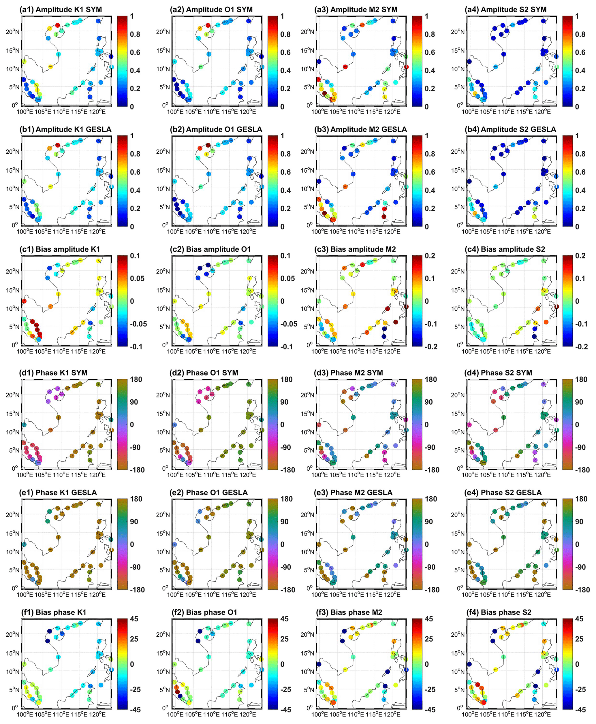
Figure 3 Amplitude (m) and phase (degree) of four tidal components K1, O1, M2, and S2 in SYM4 (SYM, a1–a4; d1–d4) the GESLA tide gauge dataset (b1–b4, e1–e4); and the model bias compared to GESLA (c1–c4, f1–f4).

FES2014b is used to provide the tidal forcing at the lateral boundaries of our numerical domain, located outside the SCS (Fig. 1a). FES2014b assimilates satellite and in situ sea surface elevation data, allowing it to be very close to observations, as shown by Piton et al. (2020) over the Gulf of Tonkin. We therefore also use it, complementary to GESLA tide gauge data, to evaluate the tidal solution produced by our model over the inner open-sea domain. In Fig. 4 we show the observed and simulated tidal amplitude and phase for K1, O1, M2, and S2, the four principal tidal components in the SCS region. The spatial distribution of tidal constituents obtained from SYM4 and from FES2014b is similar to the study of Phan et al. (2019). Diurnal tides prevail over the Gulf of Tonkin, the Gulf of Thailand, and the southwestern SCS. Mixed tides (mainly semi-diurnal tides) prevail along southern China, the northwestern coast of Borneo and the continental shelf of the Mekong delta. For those four tidal components, we obtain a strong similarity both for amplitudes and phases between SYM4 and FES2014b over most of the modeled domain. As observed from the comparison with tide gauges, the most noticeable weaknesses are a small (<10 cm) underestimation of diurnal (K1 and O1) amplitude in the Sulu Sea and Gulf of Tonkin, an overestimation (∼20 cm) of semi-diurnal (M2 and S2) amplitude in the Sulu Sea, and a small overestimation of K1 amplitude off the Mekong delta. The bias of semi-diurnal tidal amplitudes in the Sulu Sea may be related to the prescribed bathymetry in the area, with many small islands separating this area from the surrounding seas.

Comparing tidal amplitude biases in SYM4 and in SYM12 shows that the high resolution significantly reduces the biases over the whole domain (see Fig. A3): the strong O1 and K1 biases in the Sulu Sea in SYM12 are reduced by ∼80 %–90 % in SYM4, and the M2 and S2 biases near the southern China and Vietnam coasts and western Borneo coast by ∼20 %–30 %. This improvement of tidal solution in SYM4 can be partly attributed to the better representation of bathymetry details, in particular in the interocean straits (see Figs. A1, A2). Comparing SYM4 results with FES2014b tidal solution, tide gauge data, and SYM12 therefore shows that SYM4 realistically reproduces the tidal solution in the SCS, both in the open sea and in the coastal area, and that the high resolution helps to improve the realism of this tidal solution.

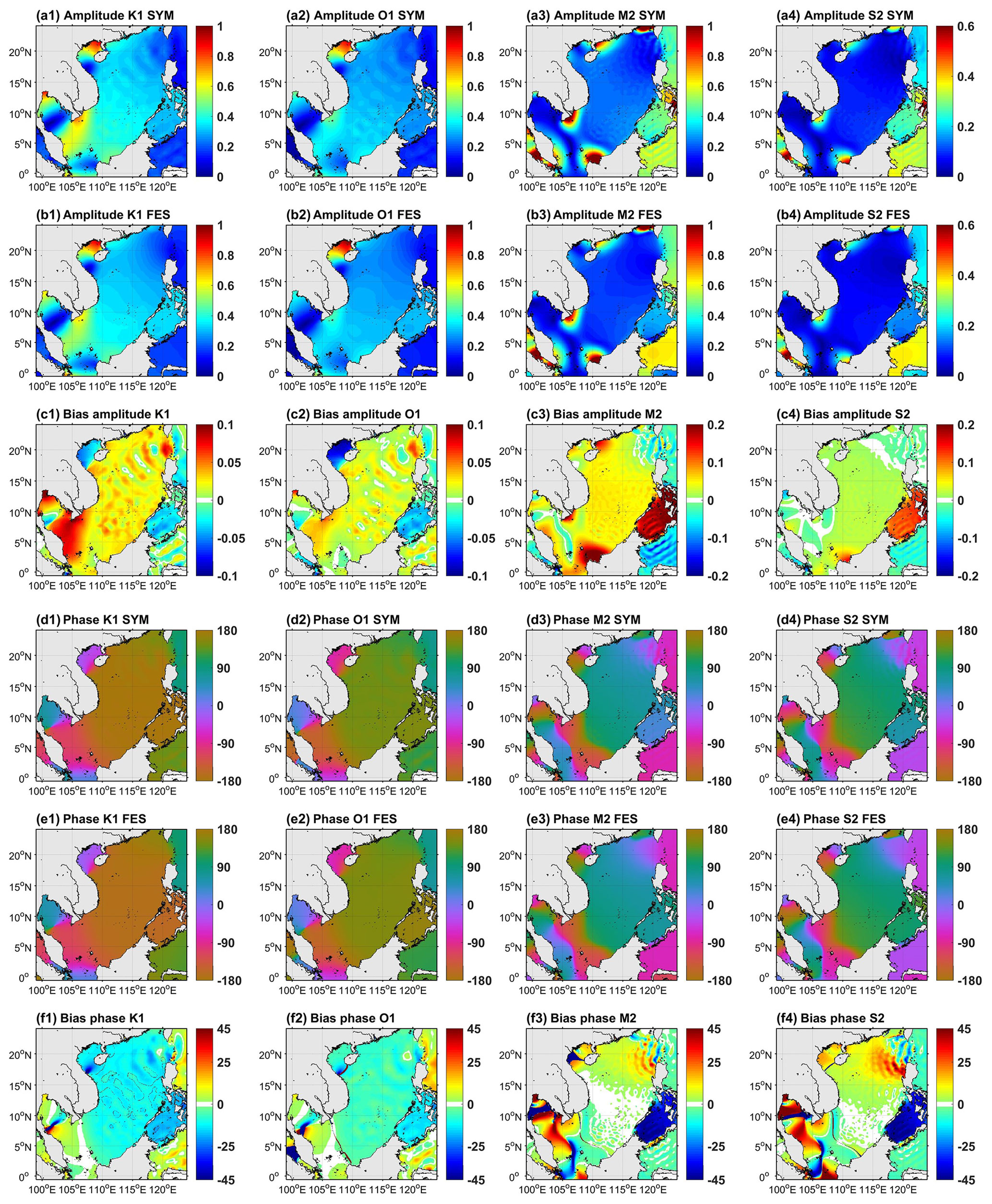
Figure 4 Amplitude (m) and phase (°) of four tidal components K1, O1, M2, and S2 in SYM4 (SYM, a1–a4, d1–d4), the global tidal product FES2014b (FES, b1–b4, e1–e4), and the bias in SYM4 compared to FES2014b (c1–c4, f1–f4).

4.1.2 Seasonal cycle of sea surface temperature, salinity, and elevation

We show in Fig. 5 the seasonal cycle (Fig. 5a, c, e) and the interannual variations (Fig. 5b, d, f) of SST, SSS, and SLA computed from model outputs (for SYMPHONIE as well as COPERNICUS, INDESO, GLORYS, and OFES) and from the corresponding satellite observations. Table 3 shows the corresponding bias, NRMSE, and correlation coefficients.

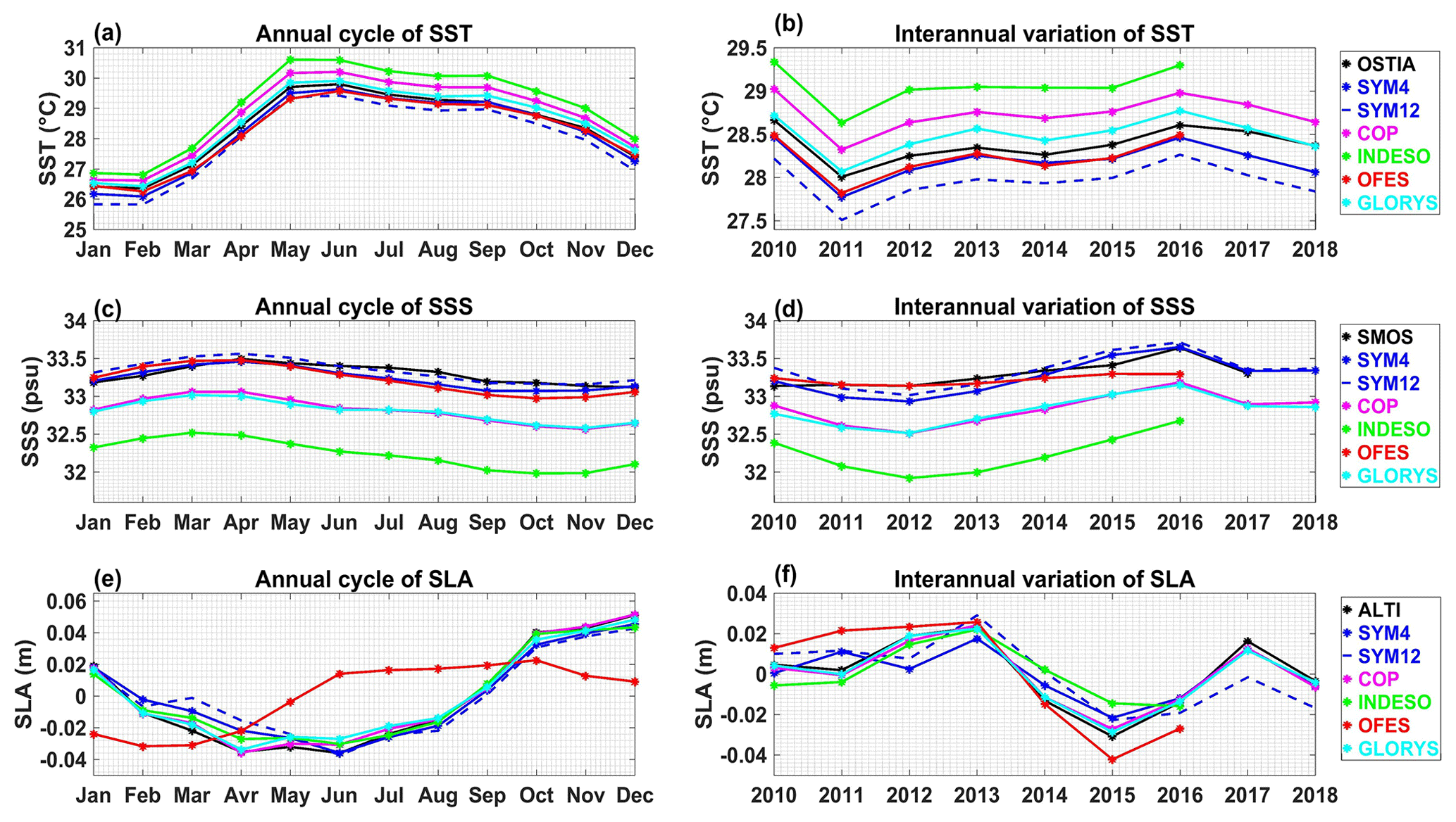
Figure 5 Time series of climatological monthly mean (a, c, e, computed over 2010–2016, the period common to all models) and yearly mean (b, d, f, over 2010–2018, except for OFES and INDESO, which are available only until 2016) of SST (°C, a, b), SSS (psu, c, d) and SLA (m, e, f) averaged over the SCS domain, computed from different models (SYM4, blue; SYM12, dashed blue; COPERNICUS, magenta; INDESO, green; OFES, red; GLORYS, cyan) and from satellite observations (OSTIA, SMOS, and ALTI, black).

The annual cycle of SST averaged over the SCS (Fig. 5a) is very well simulated in SYM4, with a highly significant correlation (R=0.99 and p value p<0.01, corresponding to a significance level higher than 99 %) and a small NRMSE (5.7 %) between SYM4 outputs and OSTIA and a slight bias of −0.18 °C for the period 2010–2018. In all datasets, the monthly climatological cycle of SST reaches its maximum value in May or June (spring–summer) and decreases to its minimum in January or February (winter). This monthly climatological SST agrees with the study of Prasanna Kumar and Seemanth (2011), who observed the same SST annual cycle by analyzing hydrographic WOA05 (World Ocean Atlas 2005) data.

The SYM4 SSS seasonal cycle (Fig. 5c) also shows a good agreement with SMOS data, with a highly significant correlation of 0.91 (p<0.01), a low NRMSE equal to 19 %, and a slight negative bias (−0.04 psu). In both model and data, the average SSS is at its maximum in April (spring), with values of 33.47 psu in SYM4 and 33.52 psu in SMOS, and its minimum from September to December (autumn), with values of 33.07 psu in SYM4 and 33.17 psu in SMOS. This significant seasonal variation of SSS in the SCS, with high salinity in winter–spring and low salinity in summer–autumn was also obtained by Kumar et al. (2010) and Zeng et al. (2014).

The annual cycle of SLA obtained with SYM4 and ALTI data during the period 2010–2018 shows a minimum value in spring–summer (June) with −0.033 m both for SYM4 and ALTI (Fig. 5e). The SLA reaches its highest value in winter (December) with 0.039 and 0.049 m, respectively, for SYM4 and ALTI. SYM4 outputs and the altimeter measurements have a highly significant correlation (R=0.97, p<0.01) and a small NRMSE value (10 %). The simulated monthly climatological SLA is also in agreement with Shaw et al. (1999) and Ho et al. (2000); using TOPEX/Poseidon altimeter data, they both concluded on a higher SLA in winter and lower SLA in summer over the SCS.

We then show the simulated and observed maps of SST, SSS, and SLA climatologically averaged over the boreal winter (December, January, and February, DJF) and summer (June, July, and August, JJA) for SYM4 (Fig. 6) and the corresponding bias for the six simulations (Fig. 7).

In both winter and summer, SYM4 SST is very close to observations, with highly significant spatial correlation (respectively R=0.99 and 0.84 in winter and summer, p<0.01) and similar ranges compared to OSTIA (Fig. 6a, b). In winter, SYM4 shows an average negative bias of −0.28 °C, and colder zones offshore southern Vietnam and in the northern basin. In summer (Fig. 6c, d), the average negative bias is reduced to −0.17 °C, and the simulation produces a SST colder than OSTIA in the northern SCS near Taiwan, off the southern Vietnamese coast, along the Mekong delta, and in the Sulu and Celebes seas (see Fig. 1a). On the other hand, simulated SST is warmer in the Gulf of Tonkin, Gulf of Thailand, and the southern basin.

The SYM4 spatial distribution of SSS also shows a highly significant spatial correlation with SMOS for both seasons (R=0.88 and 0.84 psu in winter and summer, respectively, p<0.01). SYM4 has a positive bias in winter (0.05 psu) and a negative bias in summer (−0.1 psu). In winter (Fig. 6e, f), the Chinese and Vietnam coastal zones and the Gulf of Thailand are fresher in SYM4 than in SMOS data, whereas the center of the basin and the southern Gulf of Tonkin are saltier. In summer (Fig. 6g, h), we obtain a significantly lower SSS at the big river mouths (Pearl River, Red River, Mekong River), in the Gulf of Thailand, and in the Malacca Strait in model outputs compared to SMOS. SMOS, with a resolution of 25 km, might not be able to capture these salinity changes in the coastal zone.

In both winter and summer, the simulated and observed seasonal mean spatial distributions of SLA show a highly significant correlation (R=0.97, p<0.01, Fig. 6i, j, k, l). SYM4 shows very weak negative seasonal biases in SLA compared to ALTI (−0.008 m in winter and −0.003 m in summer). In the Gulf of Thailand, the simulated SLA is lower in winter and higher in summer compared to ALTI. Regarding the geostrophic currents, we obtain great similarities between the model and ALTI. In winter when the northeastern monsoon dominates, two cells of cyclonic gyre cover the whole basin, one near Luzon and another at the Sunda shelf. In summer, with the southwest monsoon, most of the SCS geostrophic currents reverse and flow northeast. The geostrophic currents are most intense at the Sunda shelf zone (see Fig. 1a) in winter. In summer, we observe strong geostrophic flows at the southern Vietnam coast and to the east of the Malaysian coast. The intensities and directions of those seasonal geostrophic currents are consistent with previous studies (e.g., Da et al., 2019; Y. Wang et al., 2006).

Last, Fig. 8i, j shows the observed TSG-Alis SST and SSS during spring–summer 2014 and the corresponding co-localized simulated SSS and SST. Again, SYM4 shows a strong similarity with TSG-Alis data, with correlation coefficients of 0.70 and 0.82 (p<0.01) for SST and SSS, respectively, during this sixth year of the simulation.

Table 3 Bias, correlation coefficients, and NRMSE values (for the climatological monthly annual cycle and interannual yearly time series (in italics) shown in Fig. 5) for the SST, SSS, and SLA simulated by SYMPHONIE, OFES, INDESO, COPERNICUS, and GLORYS compared to satellite observations (OSTIA, SMOS, and ALTI, respectively) and for the climatological monthly annual cycle of simulated MLD shown in Fig. 9 compared to Argo data. The period over which indicators are computed is indicated below the model's name. Values in italics correspond to the correlation coefficients and NRMSE for interannual yearly time series.

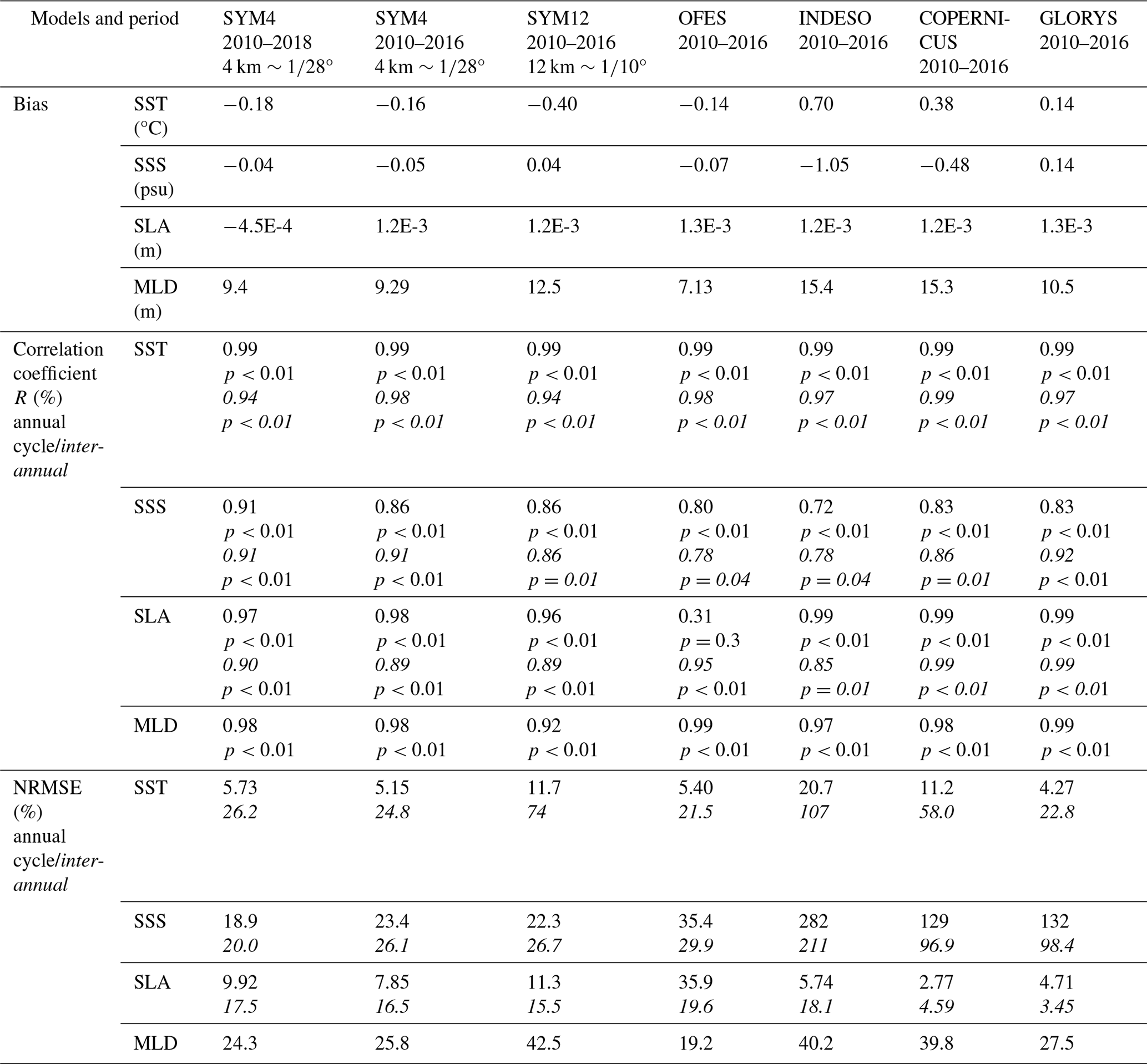
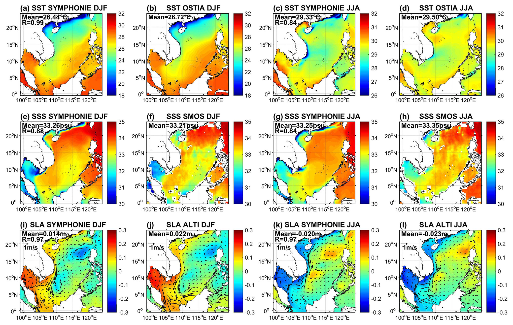
Figure 6 Spatial distribution of winter (DJF) and summer (JJA) climatologically averaged SST (°C, a, b, c, d), SSS (psu, e, f, g, h), SLA (m), and geostrophic current (m s⁻¹, i, j, k, l) in SYM4 outputs and corresponding satellite observations over 2010–2018. R stands for the spatial correlation coefficient (here the p value is always smaller than 0.01).

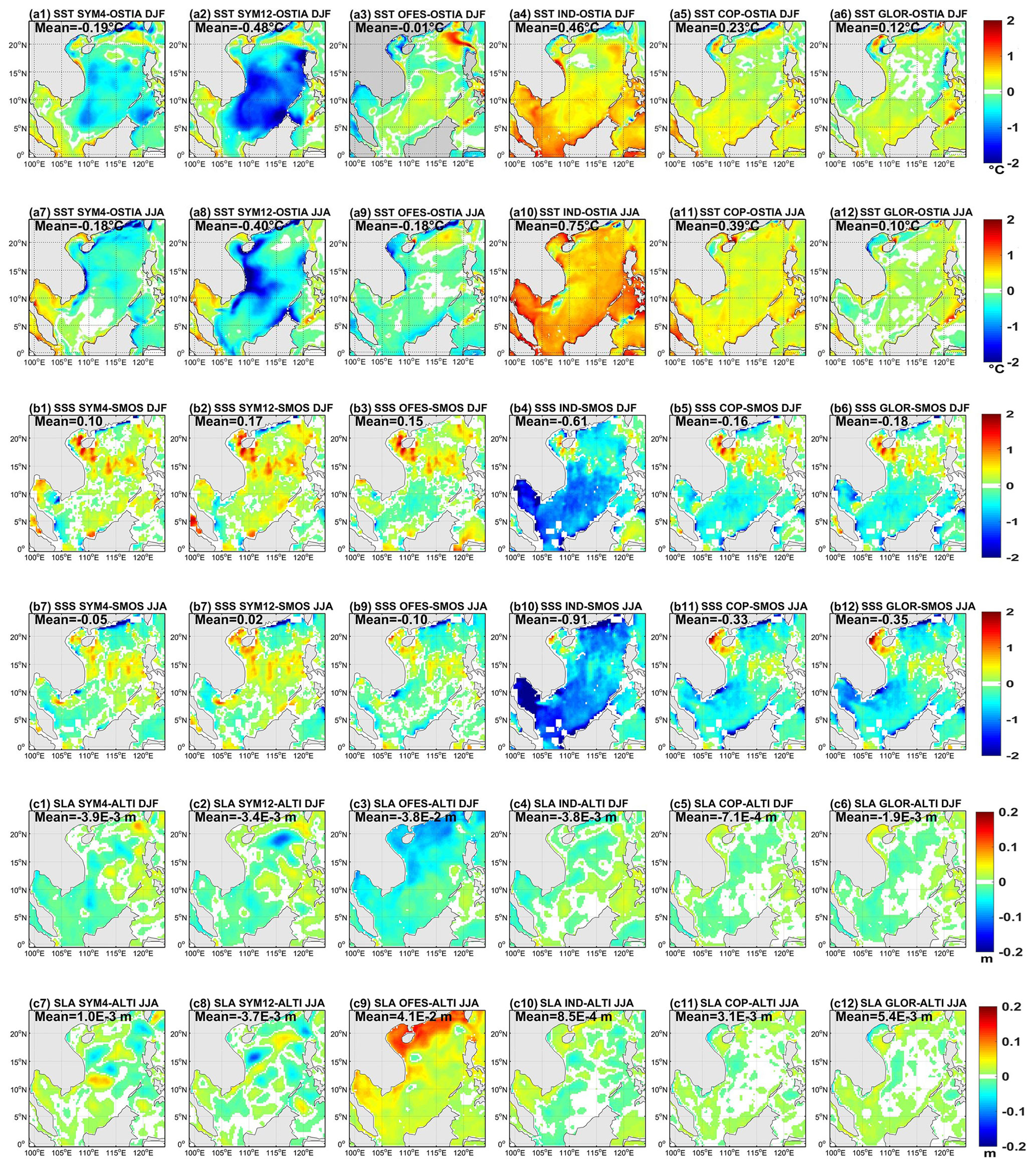
Figure 7 Maps of biases between models and satellite datasets averaged in winter (December, January, February, DJF) and summer (June, July, August, JJA) during the period 2010–2016 for SST (°C, compared to OSTIA, a1–a12), SSS (psu, compared to SMOS, b1–b12), and SLA (m, compared to ALTI, c1–c12).

4.1.3 Interannual variations of sea surface temperature, salinity, and elevation

We obtain a highly significant correlation coefficient between SYM4 and OSTIA (R=0.94, p<0.01) regarding yearly SST interannual variations (Fig. 5b). The yearly −0.18 °C SST bias is nearly constant over the period and the NRMSE is 26 %. From 2010 to 2018, the averaged yearly SST over the basin reaches its highest values in 2010 and 2016 (28.47 and 28.46 °C, respectively). This is consistent with the study of Yu et al. (2019), who found a co-occurrence between those SST positive anomalies peaks and El-Niño events in 2009–2010 and 2015–2016 (see the NOAA ONI time series available at https://origin.cpc.ncep.noaa.gov/products/analysis_monitoring/ensostuff/ONI_v5.php, last access: 18 August 2023). The minimum of averaged SST (27.77 °C) occurs in 2011, corresponding to the 2011–2012 La Niña event. Yu et al. (2019) obtained the same interannual time series by analyzing MODIS satellite-derived SST data for the period 2003–2017.

The simulated interannual variations of yearly SSS (Fig. 5d) show a highly significant correlation (R=0.91, p<0.01) and a rather low NRMSE value (20 %) with satellite data. There is a significant increase in the annual averaged SSS over the SCS between 2012 to 2016, both in SYM4 outputs and SMOS data. Over the period 2010–2017, the SSS reaches a low value in 2012 (32.93 psu for SYM4, 33.14 psu for SMOS), then increases continuously until a maximum value in 2016 (33.65 psu for SYM4, 33.64 psu for SMOS). The freshening until 2012 and strong salinification during the following 4 years are in agreement with observations of Zeng et al. (2014, 2018), who revealed that 2012 was the year with the lowest recorded value of SSS in the SCS over a 50-year period and that the SSS then increased from late 2012 to 2016.

In terms of SLA interannual variations, SYM4 and ALTI show strong similarities with a NRMSE equal to 17.5 % (Fig. 5f) and a highly significant correlation (R=0.90, p<0.01). During the studied period, the overall averaged SLA is at its maximum in 2013 (0.017 m in model outputs and 0.023 m in ALTI) and minimum in 2015 (−0.02 m in SYM4 and −0.03 m in ALTI).

4.1.4 Comparison with other models

SYM4 performances in representing sea surface characteristics are also compared with other numerical datasets over 2010–2016, the period common to all simulations (Figs. 5 and 7 and Table 3). The most striking weaknesses are an underestimation of SST (−0.4 °C) in SYM12, overestimation of SST (0.7 °C) and underestimation of SSS (−1.1 psu) in INDESO, and an incorrect representation of the SLA seasonal cycle in OFES (correlation of 0.31). Apart from this, all models compare well with observations in terms of bias, seasonal cycle, interannual variability, and spatial variability. Moreover, SYM4 is always in the upper performance range for bias, correlation coefficients, and RMSE. In comparison with other models and with SYMPHONIE at 12 km resolution, SYM4 thus shows a good performance in simulating the seasonal cycle and interannual of surface characteristics and performs as well or even better than models that include assimilation (GLORYS and COPERNICUS).

Those comparisons of SYM4 SST, SSS, and SLA time series and spatial fields with observations dataset and other simulations available from models at coarser resolution, including SYMPHONIE, therefore shows the added value of our high-resolution simulation in realistically reproducing the annual cycle and interannual variations and the seasonal spatial distributions of SCS surface hydrological characteristics and circulation over the period 2010–2018.

4.2 Water mass characteristics

We hereafter examine the performance of SYM4 in simulating the vertical distribution of water mass temperature and salinity properties. For this we compare model results with Argo and glider observations. Figure 8a–h show the co-localized simulated and observed temperature and salinity profiles, their mean value, and the bias between model and data.

We obtain a strong agreement between the simulated and observed temperature and salinity profiles both for Argo floats (over the period 2009–2018) and glider (winter–spring 2016) outputs (Fig. 8a–h). In particular the maximum salinity observed in the intermediate water mass, corresponding to the Maximum Salinity Water (MSW), is well reproduced by SYM4. In general, modeled temperatures are lower than measured temperatures, with a negative bias in the whole water column (Fig. 8b,f). The highest biases are located in the subsurface layer (50–200 m), with maximum biases of −1.2 °C compared to Argo data and of −1.5 °C compared to glider data. Under 200 m, the temperature bias is stable, varying around 0.2–0.5 °C compared to Argo floats and 0.7–1 °C compared to glider data. Model results show a general very low positive salinity bias compared to Argo and glider data below 200 m. A higher salinity bias is obtained in the subsurface layer: 0.2 psu compared to Argo data (Fig. 8d) and 0.3 psu compared to glider data (Fig. 8h). Therefore, our simulation accurately represents the various SCS water masses characteristics over the water column. Moreover, it is noteworthy that in 2016, i.e., the seventh year of simulation, those characteristics are reproduced without a significant drift.

SYM4 also shows a good performance in reproducing the temperature and salinity vertical distribution in comparison with other numerical datasets. Temperature and salinity profiles averaged over the zone 12–18° N, 112–118° E and the period 2010–2016 are shown in Fig. 10a. COPERNICUS and GLORYS profiles are closest to Argo thanks to the assimilation. Concerning the models without assimilation, INDESO shows the lowest temperature bias (maximum 0.4 °C at 100–150 m depth) compared to Argo. Higher temperature biases are observed with SYM4 ($\sim -\mathrm{1.5}\mathit{°}$C at 50–100 m depth) and OFES ($\sim -\mathrm{0.7}\mathit{°}$C at 800 m). The strongest biases in temperature profiles are obtained from SYM12, with negative bias of −3.5 °C at 50 m depth and a positive bias of 0.8 °C at 1000–1200 m depth. Regarding the salinity, SYM4 shows the lowest bias for the upper 0–300 m layer (∼0–0.3 psu), while INDESO shows a strong surface fresh bias (up to 0.8 psu), OFES and SYM12 overestimate and underestimate the salinity maximum (by ∼0.5 psu at 100–200 m depth for OFES and by −0.17 psu for SYM12), respectively. Underneath 200 m, all models present low salinity biases in comparison with observation, while OFES shows the strongest bias ($\sim -\mathrm{0.1}$ psu at 500 m).

Argo floats and glider and model data show water mass characteristics in agreement with previous studies done on water masses over the SCS (Uu and Brankart, 1997; Rojana-anawat et al., 2001, 2000; Saadon et al., 1999a, b) and the Pacific (Talley et al., 2011) (Fig. 8a–h). In the upper layer (0–50 m), we observe both the Open Sea Water (OSW), characterized by salinities of 33–34 psu and temperatures of 25–30 °C, and the Continental Shelf Waters (CSW) with low salinities (<33 psu) and temperatures between 20 and 30 °C (depending on the season). The 50–100 m layer is characterized by the mixing between the Northern Open Sea Water (NOSW) and the Pacific Ocean Water (POW) during winter. The NOSW has salinities of 34–34.5 psu and temperatures of 23–25 °C. The POW is saltier with salinities of 34–35 psu and temperatures of 25–27 °C. Deeper, at 100–200 m, the MSW is characterized by temperatures between 15–17 °C and salinities between 34.5 and 35 psu and is a property of the equatorial regions (Rojana-anawat et al., 2000). Below the MSW, from 200–1000 m, the North Pacific Intermediate Water (NPIW) and Pacific Equatorial Water (PEW) are flowing with temperatures and salinities between 5–13 °C and 34–35 psu, respectively. The Deep Water (DW), below 1000 m, is identified by temperatures of 2–5 °C, and salinities of 34.3–34.7 psu. Temperature profiles located in the Sulu Sea do not follow those characteristics in the deep layers, both in Argo and model outputs, showing temperature varying from 7 to 10 °C below 700 m. This marginal sea, nearly isothermal, indeed possesses unique water characteristics, with a potential temperature varying around 9.8 °C below 1000 m (Wyrtki, 1961; Chen et al., 2006; Gordon et al., 2011), much higher than those of neighboring seas such as the SCS, the Celebes Sea and the western Pacific (Qu and Song, 2009).

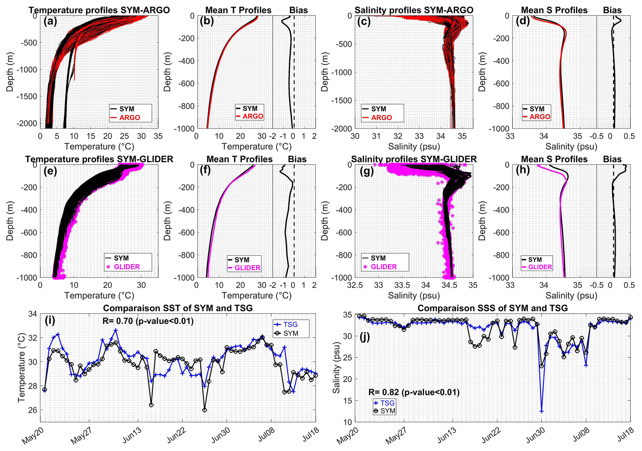
Figure 8 Temperature (°C) and salinity (psu) vertical profiles (all profiles, mean profiles, and mean bias between model and observations) from SYM4 outputs (black) compared with Argo floats (a, b, c, d, red) and glider measurements (e, f, g, h, magenta). (i) SST (°C) and (j) SSS (psu) from SYM4 (black) and TSG-Alis data (blue).

4.3 Mixed-layer depth

The seasonal distribution of simulated mixed-layer depth (MLD) in the SCS basin is evaluated by comparison with values computed from Argo profiles. The MLD is calculated based on a 0.5 °C temperature criteria, corresponding to the temperature difference between the near-surface and the MLD.

Figure 9 shows the winter (DJF) and summer (JJA) spatial distributions of the co-localized simulated (in SYM4) and observed MLD at Argo locations (in space and time), as well as the simulated and observed time series of monthly mean MLD averaged over the Argo points over the SCS. Spatial distributions of SYM4 MLD are close to observed values. Observed and simulated MLD are deeper in winter (varying between ∼80 m in the north and ∼30 m in the east, Fig. 9a, b) and shallower in summer (varying between ∼50 m in the south and ∼20 m in the north, Fig. 9d, e). The simulated MLD in both seasons are in general shallower than MLD obtained from Argo profiles, with bias locally reaching 20 m in DJF (Fig. 9c, f). This shallower MLD explains the slight temperature underestimation and salinity overestimation around ∼50 m depth (Fig. 9b, d). The average bias over the area and 2010–2018 period is equal to 9.4 m (Fig. 9g) and is stronger for higher values of MLD in winter (e.g., $\sim -\mathrm{40}$ m in January 2012). This bias is stable over the 9 years of analysis (Fig. 9g), indicating that there is no drift in terms of simulated MLD. Moreover, the observed temporal variability of MLD is well reproduced by SYM4, with a 0.91 (p<0.01) highly significant correlation between the simulated and observed interannual time series of monthly MLD.

Figure 10f illustrates the climatological seasonal cycle of MLD over the zone 12–18° N, 112–118° E and the period 2010–2016 for all modeled outputs compared to Argo. All models underestimate the MLD (Table 3), but simulate similar annual evolution of MLD, with highly significant correlation between the simulated and observed climatological monthly time series (R>0.92, p<0.01). The deepest MLD is observed in winter and the shallowest in April–May. OFES shows the smallest underestimation and NRMSE (7.3 m, 19 %), followed by SYM4 (9.10 m, 25 %). The strongest biases and NRMSE are obtained from SYM12 (12.5 m, 42 %), INDESO (15.6 m, 41 %), and COPERNICUS (15.5 m, 40 %).

This systematic underestimation of simulated MLD, stronger for higher values of MLD, could be partly related to the underestimation of wind speed. All models use bulk formulae from Large and Yeager (2004), and five of the six simulations compared here use outputs from ECMWF analysis (SYM4 and SYM12, INDESO, COPERNICUS) or reanalysis (GLORYS) as atmospheric forcing, while OFES uses JRA55 outputs (Table 1). Compared to QuikSCAT, ECMWF analysis, and reanalysis indeed underestimate sea surface wind speed (by ∼1 m s⁻¹ on average over the region for the analysis, Fig. A4). More generally, Herrmann et al. (2020, 2022) showed that global and regional atmospheric models underestimate sea surface wind speed over the SEA region. Wang et al. (2020) showed that both ERA-Interim (produced by ECMWF) and JRA55 underestimate wind over the South China Sea with a smaller bias in JRA55 (0.22 m s⁻¹ over the period 1988–2015) than in ECMWF (0.62 m s⁻¹). This underestimation of wind speed in forcing datasets, weaker in JFRA55, partly explains first why all models underestimate the MLD, and second why OFES, which uses JRA55, produces the closest MLD to observations (Fig. 10f). Moreover, as shown by Tréguier et al. (2023), MLD biases as well as their differences among models may also be due to the model formulation, parameterizations, and resolution, whose shortcomings vary between models, including horizontal and vertical resolutions, inclusion of tides, vertical mixing parameterization, and advection schemes. Gaube et al. (2019), for example, showed that mesoscale eddies, whose representation depends on those formulations, modulate the MLD. Indeed, though SYM4, SYM12, and COPERNICUS (which provides the initial and lateral oceanic boundary conditions to SYM4) use the same atmospheric conditions, the MLD underestimation is weaker in SYM4 than in SYM12 and COPERNICUS. This suggests first that the MLD underestimation in SYM4 can also be explained by the MLD underestimation of the initial and entering profiles provided by COPERNICUS, and second that SYM4, due to different formulations, in particular its high resolution, is able to partially correct the stratification of these profiles.

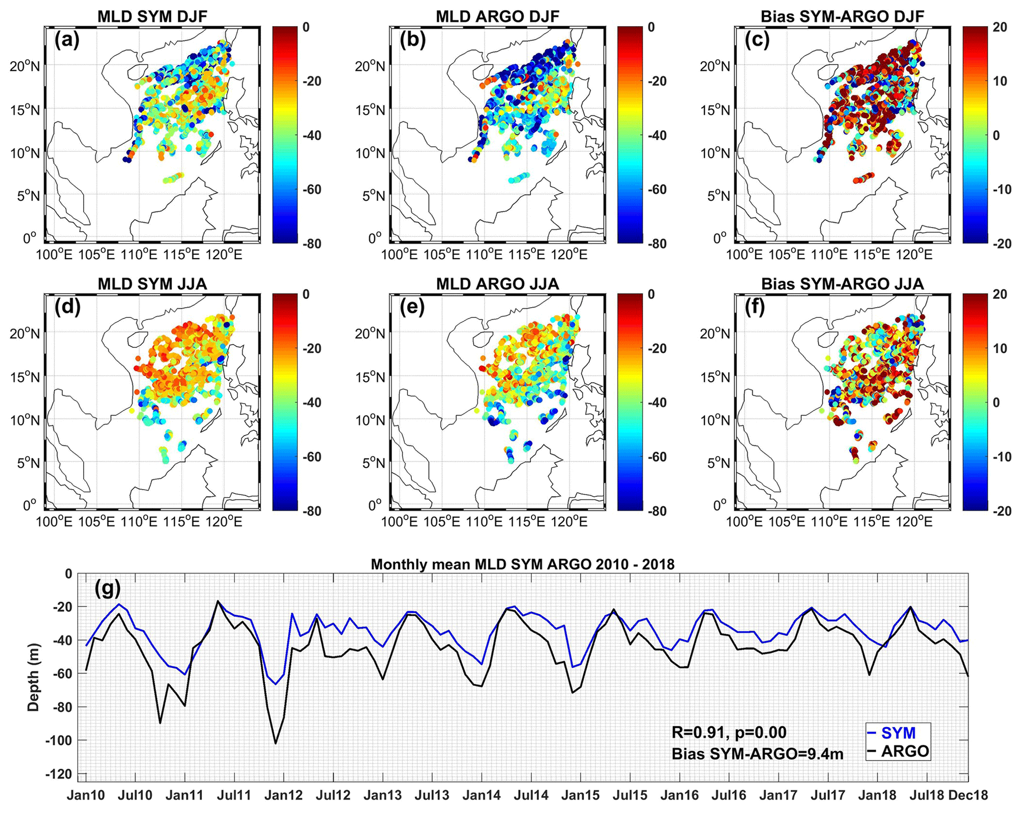
Figure 9 Seasonal distribution of MLD (m) from (a, d) SYM4 and (b, e) Argo data and their bias (c, f) in winter (a, b, c) and summer (d, e, f) over 2010–2018. (g) Time series of monthly MLD (m) averaged over the domain in SYM4 and Argo data.

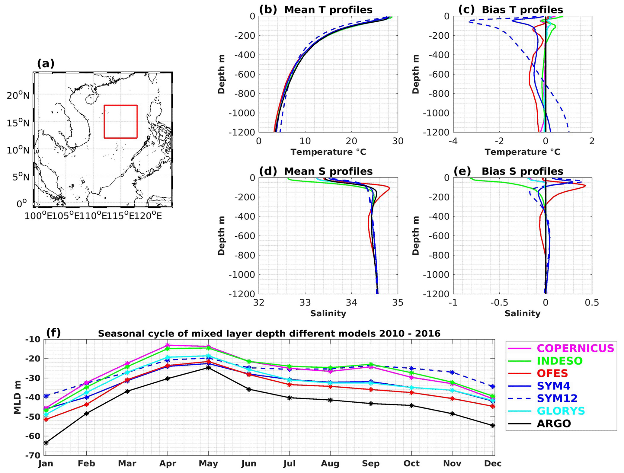
Figure 10 (a) Comparison zone (red box, 12–18° N, 112–118° E). Simulated (SYM4, SYM12, COPERNICUS, INDESO, GLORYS, and OFES) and observed (Argo) temperature (b, °C) and salinity (d, psu) profiles averaged over the comparison zone and 2010–2016 and their biases (c, e) compared to Argo. (f) Climatological monthly time series of simulated and observed mixed-layer depth over the comparison zone and the period 2010–2016.

5 Evaluation and analysis of SCS interocean strait water volume exchanges and SCS water budget

In this section, we first compile the available estimates of fluxes through SCS interocean straits and use them to assess the ability of our model to reproduce those fluxes. We then use the SYM4 to assess the contributions of lateral interocean, surface atmospheric and river fluxes, and internal variations in the SCS water volume budget at climatological and seasonal scales.

5.1 Evaluation of simulated water volume fluxes at interocean straits

A summary of lateral water volume transport published estimates at different SCS interocean straits is presented in Table 4. In situ measurements are more numerous for the Luzon and Taiwan straits than for the Karimata and Mindoro straits, and no direct measurements are available at the Balabac and Malacca straits. Given the complexity of bathymetry and current conditions in interocean straits, it is difficult to obtain accurate estimates of year-round transport from in situ observations. In addition to measurements, several models have thus been used to quantify those transports. For a given strait, those studies provided various results due to differences in methodology (e.g., sampling, studied period, choice of transects, model configuration, resolution, parameterizations, and forcings).

Table 4 Synthesis of lateral water volume transports (in Sv) through SCS straits obtained from previous numerical and observation studies and from our study. Positive indicates inflow and negative indicates outflow. When possible, fluxes ratio at different straits are calculated for four main straits (first column, in order of appearance, Luzon (entrance): Taiwan: Mindoro: Karimata (exits)). Values in italic font represent the flux ratios.

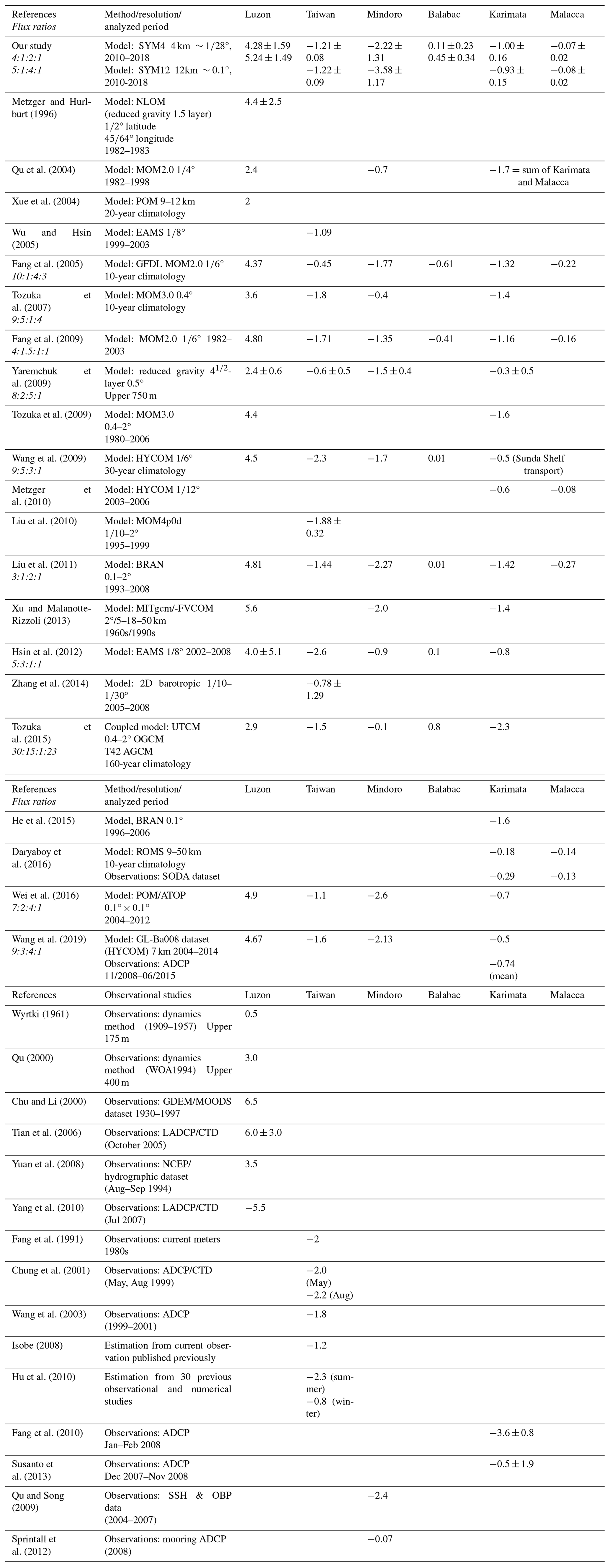
Figure 11 shows the climatological average over 2010–2018 of the lateral fluxes flowing through the SCS interocean straits, the air–sea surface fluxes, the continental river inputs, and the internal yearly variations in our simulation.

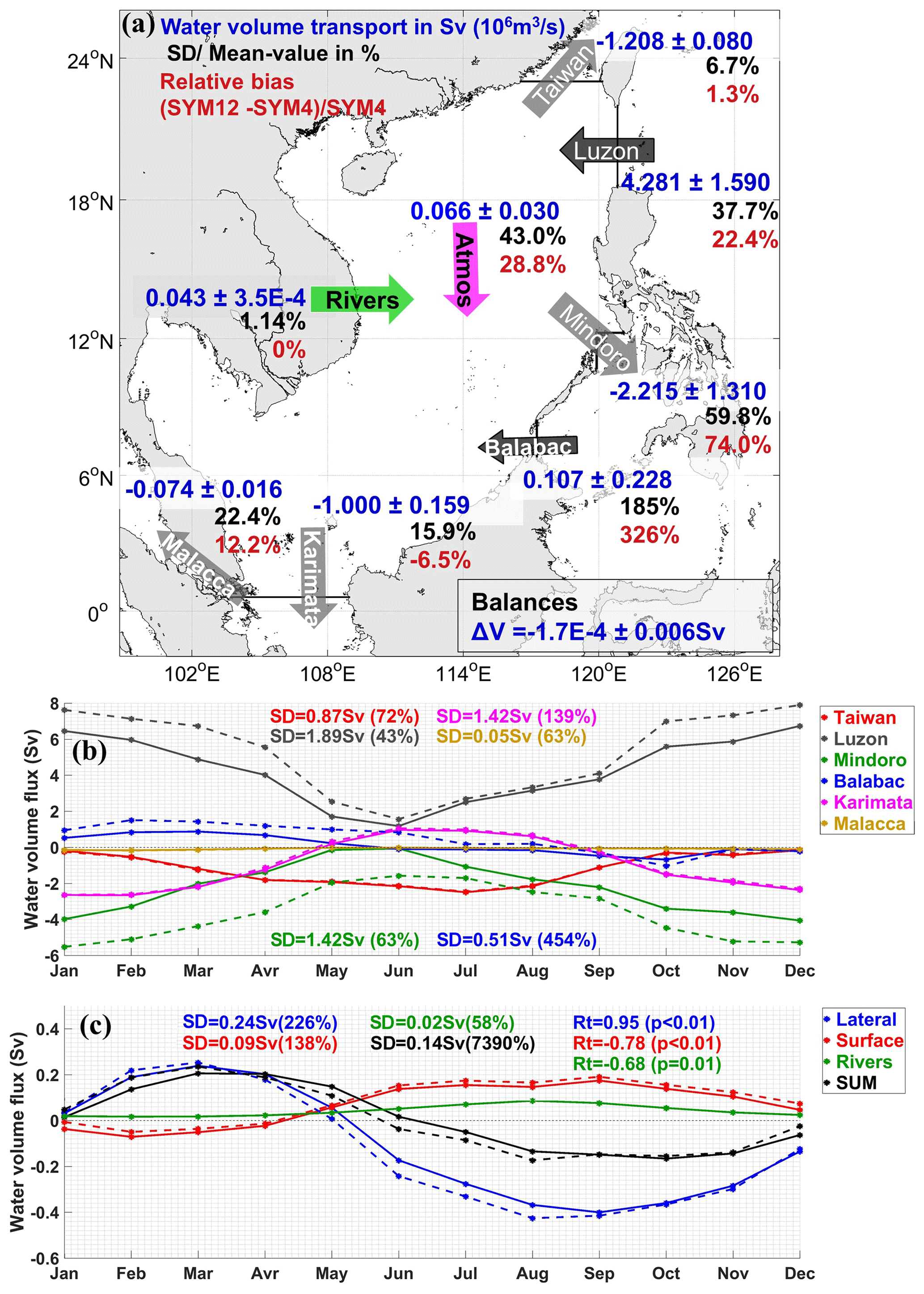
Figure 11 (a) The 2010–2018 averages and standard deviations of water volume yearly fluxes at interocean straits (black arrow is inflow, gray arrow is outflow) from the atmosphere (magenta arrow) and from rivers (green arrow). Positive and negative values correspond to inflow and outflow, respectively. In black the ratio (in %) of standard deviation and mean value is shown. In red the relative difference (in %) between the absolute value of volume transports in SYM12 and SYM4 is shown: a positive vs. negative value corresponds to a stronger vs. weaker inflow or outflow in SYM12. The yearly water volume variation in the whole SCS over 2010–2018 is provided in the bottom-right corner. Time series of monthly averages of (b) lateral water volume transport through each strait and of (c) total lateral, river, and atmospheric water volume fluxes and their sum (equal to the monthly internal variation, Eq. 1) over the SCS domain of SYM4 (solid line) and SYM12 (dashed line). SD and Rt stand for standard deviation and correlation with the sum of fluxes, respectively, calculated for SYM4.

5.1.1 Climatological mean values and seasonal cycle

In SYM4, seawater enters the SCS through the Luzon and Balabac straits and flows out of the basin via the Taiwan, Mindoro, Karimata, and Malacca straits, forming the SCSTF identified by Qu et al. (2005) (Fig. 11a). The main inflow into the SCS is from the Pacific Ocean through the Luzon Strait, with an average simulated water volume inflow of 4.3 Sv, in the range of Luzon Strait transport (LST) previous numerical estimates that vary between 2.4 and 4.8 Sv (Metzger and Hurlburt, 1996; Qu et al., 2004; Xue et al., 2004; Tozuka et al., 2007, 2009, 2015; Fang et al., 2005, 2009; Liu et al., 2011; Hsin et al., 2012; Xu and Malanotte-Rizzoli, 2013; Wei et al., 2016; Wang et al., 2019 – Table 4) and from previous observational studies that vary between 3.0 and 6.5 Sv (Qu, 2000; Chu and Li, 2000 – Table 4).

Figure 11b illustrates the simulated seasonal cycle of water volume transport through SCS interocean straits in SYM4. The LST (black line) is positive (westward) across the year, with a maximum intrusion in winter (December, 6.74 Sv) and a minimum intrusion in summer (June, 1.18 Sv), in agreement with previous numerical studies listed in Table 4 (Metzger and Hurlburt, 1996; Qu, 2000; Qu et al., 2004; Chu and Li, 2000; Fang et al., 2005; Yaremchuk et al., 2009; Liu et al., 2011; Xu and Malanotte-Rizzoli, 2013; Wang et al., 2019). Our model-averaged LST in January (6.46 Sv), August (3.14 Sv), and October (5.58 Sv) is also close to observations of Qu (2000) (5.3 Sv in January – climatology value), Yuan et al. (2008) (3.5 Sv in August 1994), and Tian et al. (2006) (6±3 Sv in October 2005), respectively.

SYM4 simulates a 1.21 Sv water volume outflow through the Taiwan Strait. This is consistent with numerical outflow estimates varying from 0.45 to 2.6 Sv (Wu and Hsin, 2005; Fang et al., 2005, 2009; Tozuka et al., 2007, 2015; Yaremchuk et al., 2009; Wang et al., 2009; Hu et al., 2010; Liu et al., 2011; Hsin et al., 2012; Zhang et al., 2014; Wei et al., 2016; Wang et al., 2019; Table 4), as well as with observational estimates of 1.8–2.0 Sv (Fang et al., 1991; Wang et al., 2003; Isobe, 2008 – Table 4). This transport is negative the whole year (Fig. 11b, red line), with a maximum 2.50 Sv outflow in July, a decrease in autumn–winter until a minimum 0.16 Sv outflow in December. These results are consistent with numerical estimations of Xue et al. (2004), Fang et al. (2005, 2009), Yaremchuk et al. (2009), Liu et al. (2011), Zhang et al. (2014), and Wang et al. (2019) and close to measurements of Wang et al. (2003), who found a maximum outflow of 2.7 Sv in summer and a minimum outflow of 0.9 Sv in winter.

At Mindoro Strait, SYM4 simulates an average lateral seawater outflow of 2.22 Sv, in agreement with estimates from previous modeling studies varying from 0.1 to 2.6 Sv (Liu et al., 2011; Wang et al., 2019; Fang et al., 2009; Yaremchuk et al., 2009; Xu and Malanotte-Rizzoli, 2013; Tozuka et al., 2007, 2015 – Table 4). The simulated outflow is also quite close to observations (2.4 Sv) analyzed by Qu and Song (2009) and stronger than in situ estimates (0.07 Sv) of Sprintall et al. (2012). Similarly to previous studies mentioned above, SYM4 simulates an outflow at Mindoro for the whole year (Fig. 11b, green line), with the maximum in December (4.05 Sv) and minimum in summer (0.06 Sv outflow in June).

In the south of the SCS, SYM4 produces a 1.0 Sv seawater outflow through the Karimata Strait, in agreement with previous numerical estimates ranging from 0.3 to 2.3 Sv (Fang et al., 2005, 2009; Yaremchuk et al., 2009; Tozuka et al., 2007, 2009, 2015; Wang et al., 2009; Metzger et al., 2010; Liu et al., 2011; Xu and Malanotte-Rizzoli, 2013; He et al., 2015; Daryaboy et al., 2016; Wei et al., 2016; Wang et al., 2019; Table 4) and slightly larger than estimates from measurements (0.50 to 0.74 Sv). The simulated annual cycle of the Karimata water volume transport (Fig. 11b, magenta line) shows a southward outflow from September to April and a northward inflow from May to August, with values ranging from −2.64 Sv in January to 0.97 Sv in June, again in agreement with previous studies (Fang et al., 2005, 2009; Xue et al., 2004; Yaremchuk et al., 2009; Liu et al., 2011; Xu and Malanotte-Rizzoli, 2013; He et al., 2015; Wei et al., 2016; Wang et al., 2019; Daryaboy et al., 2016; Susanto et al., 2013; Wang et al., 2019).

Compared to the four main straits of the SCS, the Balabac and Malacca straits show water volume transports one order of magnitude smaller (Fig. 11b), and observational studies are scarce. SYM4 produces an annual mean westward inflow of 0.11 Sv at Balabac, in agreement with the estimate of 0.1 Sv by Hsin et al. (2012), while Wang et al. (2009) and Liu et al. (2011) estimated very small inflows (0.01 Sv) and Tozuka et al. (2015) suggested a much stronger inflow (0.8 Sv). Fang et al. (2005, 2009), in contrast, proposed an eastward outflow of, respectively, 0.061 and 0.41 Sv at these channels. In SYM4, water enters at Balabac from January to May (maximum of 0.88 Sv in March, Fig. 11b, blue line) and exits from June to December (maximum of 0.68 Sv in October). Fang et al. (2005, 2009), on the other hand, obtained an outflow the whole year.

At the narrowest interocean strait of the SCS, Malacca, water flows out of the SCS toward the Andaman Sea (Indian Ocean) at a rate of 0.07 Sv in our simulation, at the low end of the range of previous estimates (from 0.08 to 0.27 Sv; Metzger et al., 2010; Fang et al., 2009; Liu et al., 2011; Daryaboy et al., 2016). The Andaman Sea receives water from the SCS all over the year in SYM4 (maximum 0.16 Sv in February, minimum 0.02 Sv in May and June, Fig. 11b, cyan line) consistent with model results of Fang et al. (2005, 2009).

Last, the water volume transport at Balabac Strait shows the strongest annual variability over the yearly cycle (Fig. 11b), with a very high standard deviation relative to the average (0.51 Sv, 454 %), followed by the Karimata (1.42 Sv, 139 %), Taiwan (0.87 Sv, 72 %), Mindoro (1.42 Sv, 63 %), Malacca (0.05 Sv, 63 %), and Luzon (1.89 Sv, 43 %) straits.

5.1.2 Vertical structure

We examine the vertical distribution of water volume interocean fluxes along the water column for the whole year, summer, and winter in SYM4 (Fig. 12).

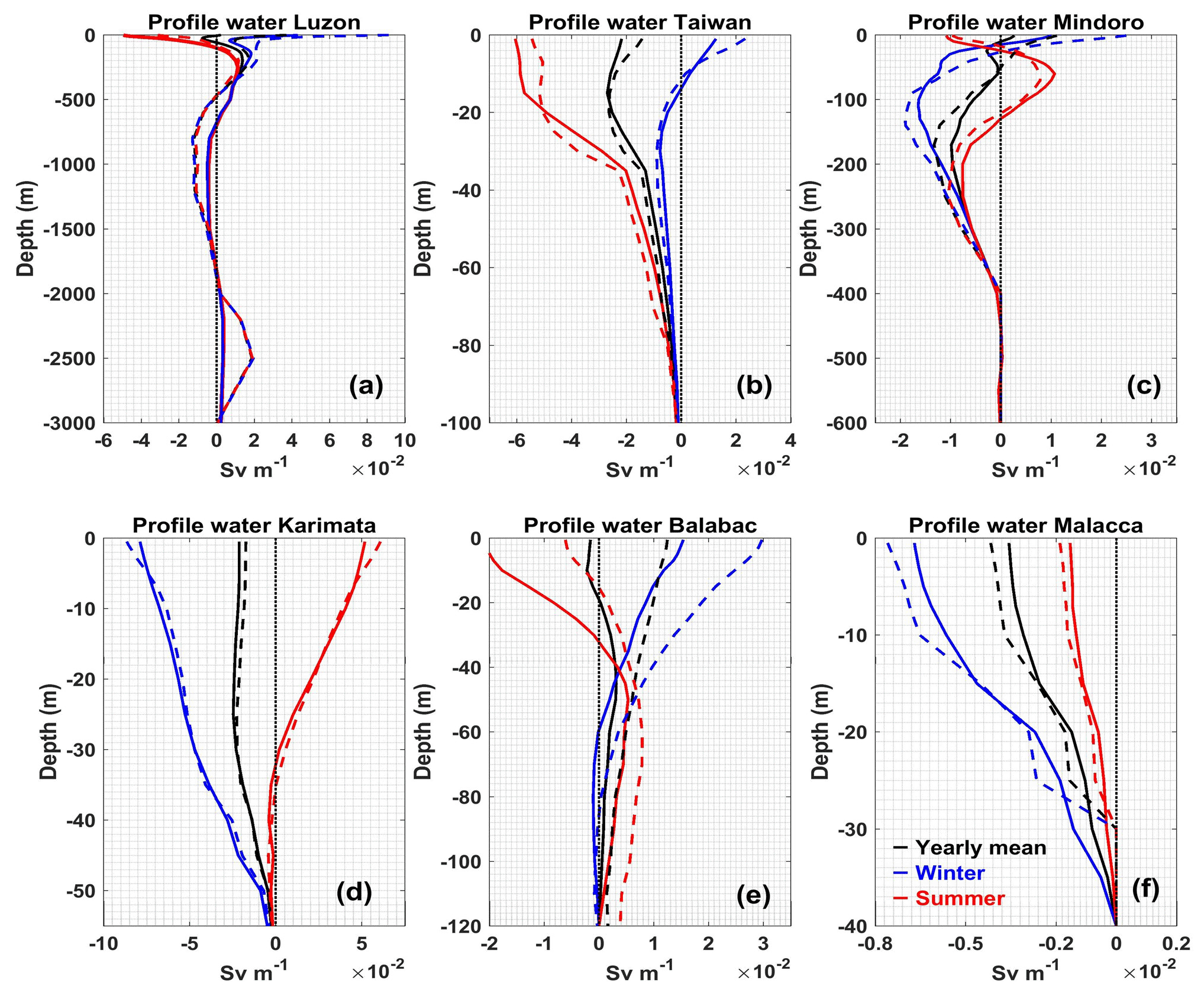
Figure 12 Yearly (in black) and seasonal (winter: December, January, and February, in blue and summer: June, July, August, in red) climatological averages over 2010–2018 of vertical profiles of water volume lateral fluxes via the six interocean straits (Sv m⁻¹) in SYM4 (solid line) and SYM12 (dashed line). Positive and negative values indicate inflow and outflow, respectively. The depth axis varies and is adapted to the depth of the strait.

At the largest and deepest strait of the SCS, the Luzon Strait, SYM4 simulates a strong seasonal variability of fluxes in the surface and subsurface layers, from 0 to 400 m (Fig. 12a). In the first 50 m, the lateral seawater flux is westward (inflow) in winter and eastward (outflow) in summer, in phase with the seasonal wind forcing (northeast monsoon winds in winter and southwest monsoon winds in summer). This seasonal variability of the surface flow is consistent with observations of Centurioni et al. (2004) obtained from Argo floats data showing an inflow in the upper 15 m from the Pacific to the SCS in winter but no inflow in summer. The yearly averaged flux is eastward for the upper 50 m. In the 50–700 m layer, summer, winter, and yearly mean fluxes are all westward, with a maximum inflow between 100 and 300 m. Until 400 m depth, inflow is stronger in winter and weaker in summer. Below 400 m depth, we do not obtain any significant seasonal variability. SYM4 produces an outflow for all seasons between 700 and 1900 m (slightly stronger in winter), then a weak inflow in the deep layer (slightly stronger in summer) from 1900 m until the bottom. Qu et al. (2004), Hsin et al. (2012), Nan et al. (2013, 2015), and Liu and Gan (2017) found the same vertical structure of water volume transport crossing the Luzon Strait using numerical methods as Li and Qu (2006) did using dissolved oxygen distribution data.

The yearly mean water volume fluxes through the Taiwan Strait are negative, i.e., northward, along the whole water column (Fig. 12b). SYM4 simulates a strong seasonal variability of vertical distribution of fluxes at this shallow strait, again triggered by the atmospheric forcing. In winter, under the northeast monsoon wind, fluxes flow southward in the surface layer (0–10 m), then underneath this depth, fluxes become northwards. In summer, under the southwest monsoon wind, fluxes are northwards from the surface to the bottom, and particularly strong between 0 and 15 m.

Regarding the Mindoro Strait (Fig. 12c), SYM4 simulates a strong seasonal variability of fluxes for the upper 300 m. Deeper than 300 m, we observe no significant seasonal variability of fluxes, which are negligible below 400 m. In winter, fluxes flow inward in the layer 0–20 m and outward between 20 and 400 m, with a maximum outflow around 120 m. In summer, we obtain a “sandwich” vertical distribution like at the Luzon Strait, with outflows in the upper layer (0–30 m, maximum at the surface) and in the subsurface layer (130–400 m, maximum near 200–250 m) and an inflow between these two layers (30–130 m, maximum near 60 m). Again, winter westward inflow and summer eastward outflow in the surface layer follow the monsoon wind direction. Below 130 m, both winter and summer fluxes flow outward, but the winter outflow is much stronger than the summer one. The annual mean flux shows a small inflow in the first 10 m and an outflow below 10 m, with local maxima at 30 and 180 m depths.

At the shallow Karimata Strait (Fig. 12d), the yearly climatological fluxes are southwards (outflow) over the full depth. Like for the Taiwan Strait, fluxes through the Karimata Strait strongly vary with the seasonal monsoon summer southwest and winter northeast winds. In summer, fluxes enter the basin above 30 m depth, then slightly flow out in the deepest layer until 55 m depth. In winter, fluxes are southwards all along the water column. This simulated seasonal variability of vertical fluxes is in agreement with in situ measurements of Fang et al. (2010), who found that the monsoon was the main factor influencing the fluxes at the Karimata Strait.

The vertical structure of fluxes across the shallow Balabac Strait also connecting the SCS with the Sulu Sea also varies strongly with the seasonal cycle (Fig. 12e). In winter, the (westward) inflow is maximum at the surface then decreases with depth. From 60 m depth to the bottom, the winter flux becomes slightly negative. The situation is opposite in summer: fluxes flow eastward (outflow) in the surface layer with a decrease with depth until 30 m, then flow westward from 30 m depth until the bottom. The annual mean fluxes are negative for the upper 20 m, then positive until the bottom (with a maximum inflow at 40 m depth).

Fluxes crossing the Malacca Strait flow westward (outflow) all year round along the whole water column, with stronger values near the surface, and a decrease with depth and stronger fluxes in winter (Fig. 12f). As the section is very shallow (40 m depth), the monsoon wind again plays an important role in the difference in seasonal flux intensity: the northeasterly wind reinforces the outflow in winter, and the southwestern monsoon reduces it in summer.

5.2 Contributions of surface, river, and lateral interocean fluxes to the SCS water volume budget

In this section we analyze the water volume budget obtained from our SYM4 simulation and quantify the contributions of each term of Eq. (1) to the internal variations of water volume in the SCS: lateral fluxes flowing through the SCS interocean straits, air–sea surface fluxes and continental inputs from rivers.

The average net seawater volume exchanged through SCS interocean straits over the period 2010–2018 in SYM4 is equal to −0.11 Sv (Fig. 11a). This net lateral loss at the domain oceanic open boundaries is balanced by the inputs from rivers and atmosphere, evaluated, respectively, at 0.04 Sv and 0.07 Sv, i.e., a total freshwater volume input of 0.11 Sv (Fig. 11a). The difference between the gain from atmosphere and rivers and the loss from straits, i.e., the water volume variation, is equal to $-\mathrm{1.7}\times {\mathrm{10}}^{-\mathrm{4}}$ Sv, equivalent to a decrease in sea level of 1.6 mm yr⁻¹ over the period 2010–2018 and negligible compared to the total water volume input (0.004 %). The SYM4 value of atmospheric freshwater flux is slightly smaller than estimates of Qu et al. (2006), who provided an annual mean value of 0.1–0.2 Sv through analyses of several datasets of precipitation (CMAP, GPCP, TRMM) and evaporation (NCEP reanalysis). Fang et al. (2009) deduced from the land discharge relation of Perry et al. (1996) an annual river flux of 0.05 Sv, close to our yearly river water volume flux. Using numerical models, Qu et al. (2006), Fang et al. (2009) and Wang et al. (2019) obtained a yearly average of total freshwater flux over the whole SCS, respectively, of 0.08 Sv (period 1950–2003), 0.11 Sv (period 1982–2003), and 0.11 Sv (period 2008–2015), quite close to SYM4 result. These previous studies assumed a null total lateral water volume flux and calculated the total freshwater flux based on the lateral salt budget and the mean salinity of the whole basin.

Figure 11c illustrates the 10-year climatological monthly averages of all the water volume fluxes exchanged between the SCS and surrounding environment in SYM4: the total interocean lateral flux, river runoff, and surface atmospheric flux and the sum of all three fluxes, which equals the internal water volume variation (Eq. 1). The total lateral flux is positive (inflows < outflows) from January to May and negative (inflows > outflows) the rest of the year. The strongest net lateral inflow occurs in March (0.24 Sv), and the strongest outflow occurs in September (−0.40 Sv). Atmospheric and river fluxes are out of phase with those lateral fluxes. Surface fluxes are negative during the winter–spring dry season (with a maximum surface loss in February, −0.07 Sv) when evaporation dominates precipitation. During the summer–autumn rainy season, precipitation becomes abundant, the surface fluxes become positive (maximum value in September 0.17 Sv), and the freshwater river flux increases from May to October with a maximum in August (0.09 Sv).

To better understand the role of the SCS in the global and regional water cycle, we analyze the sum of the water volume fluxes (Fig. 11c, black curve) exchanged yearly over the domain, equal to the water volume variation. Overall, the SCS stores water from January to June (with a maximum 0.21 Sv storage in March and April) and releases water from July to December (minimum of −0.17 Sv in October). The correlations between monthly oceanic lateral, surface, and river fluxes and the total water monthly flux are, respectively, 0.95 (p<0.01), −0.78 (p<0.01), and −0.68 (p=0.02). The lateral winter gain (and summer lateral loss) largely exceeds the atmospheric winter loss (and summer atmospheric and river gain). Moreover, the standard deviation of the climatological monthly total lateral flux (0.24 Sv) is about 3 times higher than the standard deviation of atmospheric fluxes (0.09 Sv) and 10 times higher than the standard deviation of river fluxes (0.02 Sv). Over an annual cycle, the monthly variability of the lateral flux, which is strongly driven by monsoon winds, therefore dominates the variability of the two other fluxes (atmospheric and river) and drives the annual cycle of the SCS water storage. The low variability of river fluxes compared to lateral and surface fluxes is partly explained by the use of monthly climatology river runoff for most of the rivers in SYM4, especially for huge rivers such as the Mekong and Pearl rivers.

5.3 Influence of model resolution

We showed in Sect. 4 that the use of a higher-resolution model improves the quality of the simulation in terms of ocean dynamics and water masses representation. Here we quantify the influence of this resolution on the water budget estimate. The interocean water volume transports and total water budgets computed from SYM12 are shown in Figs. 11 and 12.

The direction of averaged yearly water volume transports (inflow or outflow) are the same at all straits for SYM4 and SYM12 simulations (Fig. 11a). However, except for Karimata Strait (with a 6.5 % decrease in outflow), water volume exchanges are stronger in SYM12 than in SYM4 (from +1 % to +70 %), in particular at the two main straits: +22 % for the Luzon inflow and +70 % for the Mindoro outflow. Luzon inflow and Mindoro outflow are especially strong in March (with respective differences compared to SYM4 of 1.8 and 2.3 Sv, Fig. 11b) and over the whole water column (Fig. 12a, c, e). Conversely, differences are negligible at the Taiwan, Karimata, and Malacca straits (<10 %, Fig. 11a) throughout the year (Fig. 11b) and the column (Fig. 12b, d, f). Taiwan, Karimata, and Malacca are shallow straits with depth <100 m, while Luzon and Mindoro are much deeper straits. Though bathymetries of shallow and wide straits are not strongly affected by the resolution of the grid, the differences are considerable in deeper straits, especially in the deep narrow layers, which can partly explain this fluxes overestimation (Figs. A1, A2).

In terms of water budget, we obtain similar seasonal cycles of lateral, surface, and river water volume fluxes in SYM12 and SYM4 but slightly though significantly different values (Fig. 11c). SYM12 surface water exchanges are slightly smaller from January to April (when the ocean loses water to the atmosphere) but stronger the rest of the year (when the sea receives water), and the net atmospheric input is larger on a yearly average (29 %). This difference can be explained by the use of Large and Yearger (2004) bulk formulae: the colder SST (but the same air temperature from ECMWF) in SYM12 compared to SYM4 (Fig. 7a2, a8) results in weaker latent heat flux, hence evaporation. The total interocean lateral water outflow is consequently also larger in SYM12 all year long (+18 %), compensating for the larger atmospheric net input.

6 Conclusions

The three-dimensional hydrodynamic model SYMPHONIE was implemented over the South China Sea with high horizontal resolution and an explicit representation of tides to simulate and study the functioning, variability, and influence of ocean circulation in the SCS and their role in regional climate.

A simulation was performed at 4 km resolution over the recent 9-year period 2010–2018, using 3-hourly atmospheric forcing, daily lateral oceanic boundary forcing, nine tidal forcing components, and real-time or climatology data for 63 river discharge points. The ability of the model to reproduce the characteristics of circulation and water masses over the SCS, including tides, was evaluated through a thorough comparison with available satellite and in situ observation datasets and with simulations performed with other models at coarser resolution. The model shows good performances in terms of tidal cycle and of seasonal cycle, interannual variability, and spatial distribution of surface characteristics and circulation (SST, SSS, SLA, and associated geostrophic currents). Comparisons with Argo and glider profiles and other models showed that SYM4 accurately reproduces the vertical distributions of temperature and salinity as well as MLD. These comparisons with observational data and other models and simulations at coarser resolution therefore quantitatively show the added value of this high-resolution hydrodynamic model that includes tides for the representation and study of the spatial and temporal variability of the SCS dynamics and water masses.

One of the first objectives of this numerical tool is to study the variability of the water volume, heat, and salt budgets at different scales, precisely quantifying the contribution of each component: lateral oceanic, surface atmospheric, and river fluxes and internal variations. We implemented an online computation method, allowing us to rigorously close those budgets: over any given period, and for all the quantities studied, the sum of all fluxes is equal to the variation of the quantity over the period. We quantitatively demonstrated the added value of the online method. With offline computation based on daily outputs, NRMSE reaches 10 % to 30 % for interannual variations of yearly values of heat and salt net lateral fluxes. Moreover, the online method allows us to rigorously compute the total inflowing and outflowing fluxes at each lateral strait , contrary to the offline method that induces errors of the same order or even an order of magnitude larger than the values themselves.

This simulation was then used to provide a new quantitative insight into the SCSTF and SCS water volume budgets at the seasonal and climatological scales. Estimates over the 2010–2018 period of the water volume transports through SCS interocean straits and of their seasonal cycle and vertical distributions, and of each term of the volume budget over the whole domain were examined and compared with a synthesis of previous estimates. They were shown to be in agreement with available observational and numerical studies. According to our simulation, the SCS receives over the period 2010–2018 an annual average 4.50 Sv water input, mainly from the Western Pacific through the Luzon Strait (4.28 Sv, 95 %). The remaining input comes from the Sulu Sea through the Balabac Strait (3 %), from the atmosphere (1 %), and from rivers (1 %). The SCS releases all of this water through the other straits: half of the water flows to the Sulu Sea through the Mindoro Strait, about a quarter flows northward to the East China Sea via the Taiwan Strait (27 %), and a quarter flows southwestward to the Java Sea through the Karimata Strait (22 %). Those results are in agreement with previous modeling studies, who all reported Luzon as the main entrance and Taiwan, Mindoro, and Karimata as the main exits (see ratios provided in Table 3), though differences between quantitative estimates due to different methodologies exist. Our ratios are close to those of Fang et al. (2005), Liu et al. (2011), Wei et al. (2016), and Wang et al. (2019), who all reported Mindoro as the main exit: they estimated the distribution ranges for outflows through the Taiwan, Mindoro, and Karimata straits at 10 %–34 %, 44 %–53 %, and 11 %–30 %, respectively. Tozuka et al. (2007), Fang et al. (2009), Wang et al. (2009), and Hsin et al. (2012) reported the main exit at Taiwan strait (with respective estimates of 35 %–60 %, 11 %–37 %, and 11 %–39 %), while Tozuka et al. (2015) reported it at Karimata strait (60 %). The numerical approach valuably complements in situ observations, whose spatial and temporal coverage does not currently allow these ratios to be estimated. Obtaining in situ estimates is indeed challenging, requiring the implementation of simultaneous measurements in all these straits over a long period, but they would enable further assessment of the robustness of numerical estimates.

Taking the sum of fluxes through the Mindoro, Balabac, Karimata, and Malacca straits (following Fang et al., 2009; He et al., 2015; Wei et al., 2016), we provide a 3.2 Sv estimate for the water volume transport from the SCS into the Indian Ocean: 70 % of the total water input to the SCS is transferred toward the Indian Ocean. The analysis of the seasonal cycle of SCSTF and SCS water budgets shows that from February to July, the SCS stores water. This water gain first comes from lateral fluxes (February to April), mainly through the Luzon Strait, then to a lesser extent from rivers and atmospheric freshwater fluxes (May to July). From August to January, the SCS loses water: it receives water from the atmosphere and rivers but releases a larger amount of water through lateral fluxes, mostly through the Taiwan, Mindoro, and Karimata straits, with a peak outflow in August–September. The SCS is a source of water to the atmosphere from January to April (evaporation exceeds precipitation) and a sink from May to December. Interocean exchanges, as well as their vertical structures, show seasonal variations that weaken when depth increases and that are driven by monsoon winds. Exchanges at Luzon, Mindoro, and Karimata straits are enhanced during the autumn–winter period, from October to February, and weakened during the spring summer period, from April to September (and even reversed for Karimata), due to the opposite effects of the winter northeast monsoon winds (that favor eastward and southward flows) and of the southwest monsoon winds (that favor westward and southward flows). The situation is the opposite at Taiwan Strait, where the winter northeast monsoon weakens the northward outflow and the summer southwest monsoon enhances it. Exchanges through Luzon Strait deep layers show a stable sandwiched structure with vertically alternating inflows and outflows. Finally, seasonal variations of SCS water content are completely driven by the lateral oceanic water volume fluxes through interocean straits, themselves driven by seasonal monsoons. We showed that the use of a high-resolution vs. coarse-resolution model improves the quality of the simulation of SCS ocean dynamics and influences the water budget estimate. This 9-year SCS simulation from a high-resolution model producing a consistent closed water volume, heat, and salt budgets will now be used to examine the interannual variability of those budgets over the region in detail. Except at Taiwan Strait, interocean and atmospheric water volume fluxes indeed vary strongly on an interannual timescale: standard deviations of yearly fluxes can be of the same order of magnitude as mean values, reaching 38 % and 60 % at Luzon and Mindoro straits and even 185 % at Balabac Strait (Fig. 11a). These important variations partly explain the uncertainties in numerical and observational estimates. In addition, a decrease in SSS over the period 2011–2012 followed by an increase until 2016 were observed over the SCS by Zeng et al. (2014, 2018) and attributed to an increase in precipitation and a reduced intrusion of the Kuroshio salty water mass at Luzon Strait, followed by a decrease in precipitation and a stronger Luzon inflow. Those SSS interannual variations are reproduced well by our simulation, which will be used to examine and explain them in detail.

The simulation presented here is fully available to the interested scientific community. Using this hydrodynamical numerical tool to model and understand the SCS ocean dynamics will allow us to examine their influence on other compartments of the regional system. A coupling with a biogeochemical model (Herrmann et al., 2014, 2017) would allow us to study the functioning and variability of SCS planktonic ecosystem, which are strongly influenced by ocean dynamics (Bombar et al., 2010; Loisel et al., 2017; Lu et al., 2018). This simulation, or simulations performed over given periods of interest, could also be used to assess the dispersion of potential contaminants over the area (plastics, radioactive contaminants, etc.; e.g., Estournel et al., 2012). A coupling with a regional atmospheric model, which will allow us to consider and examine the contributions of air–sea interactions in the ocean and atmosphere dynamics in the region, is also under development over the Southeast Asia region to be integrated in the framework of the CORDEX-SEA project (Tangang et al., 2020; Herrmann et al., 2022).

Appendix A

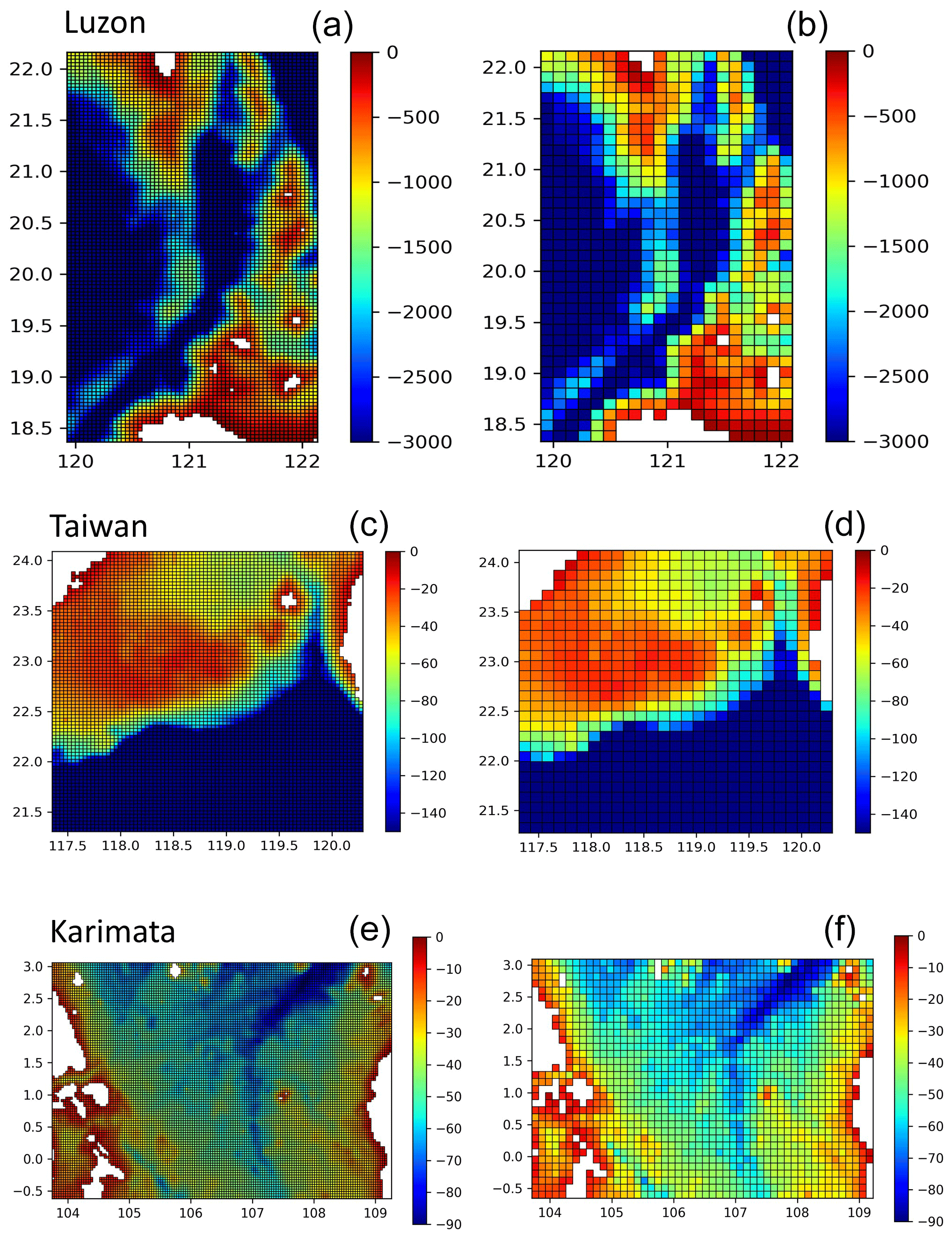
Figure A1 Bathymetries (m) and grids of interocean straits in SYM4 (a, c, e) and SYM12 (b, d, f) configurations for the Luzon, Taiwan, and Karimata straits.

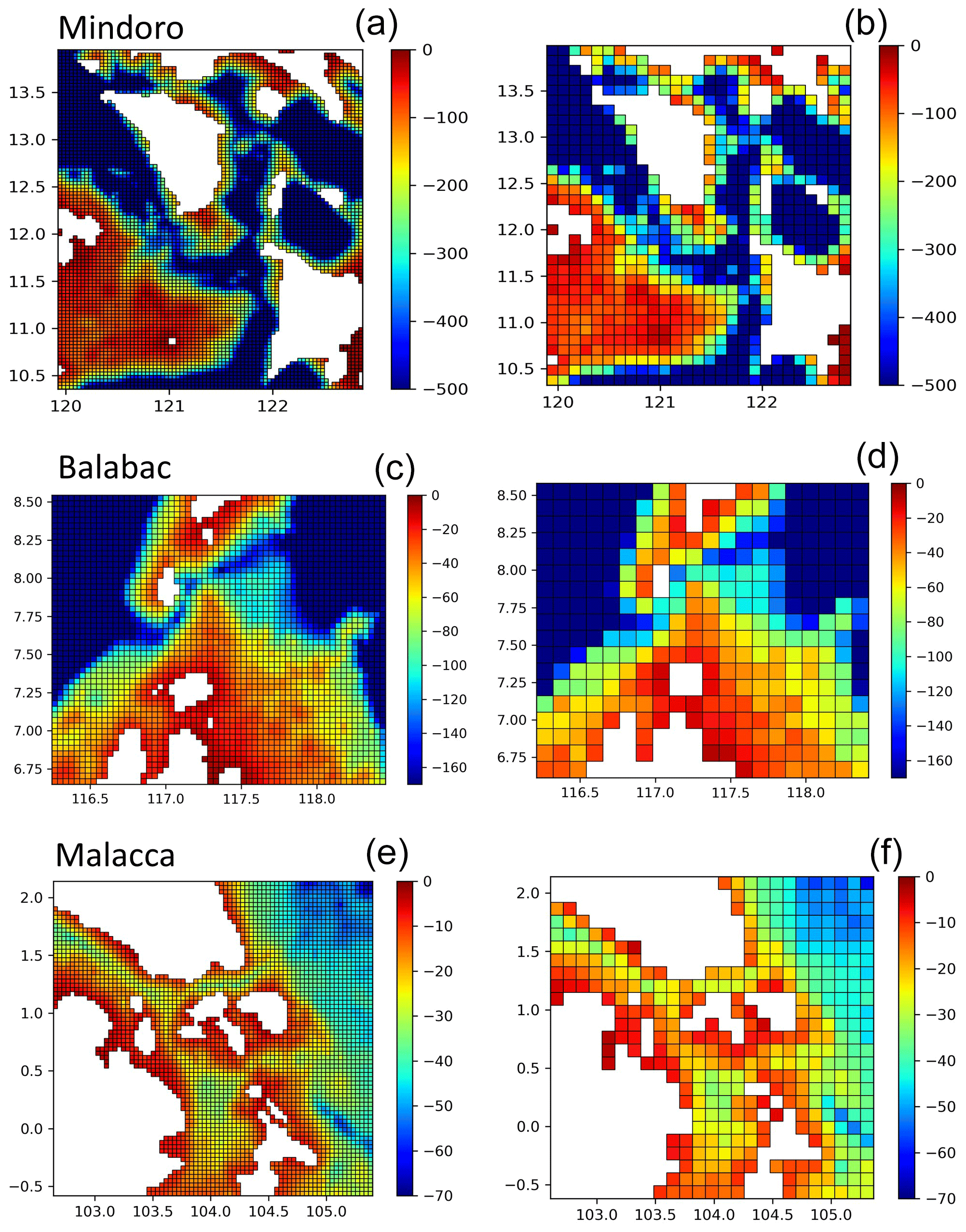
Figure A2 The same as Fig. A1 but for the Mindoro, Balabac, and Malacca straits.

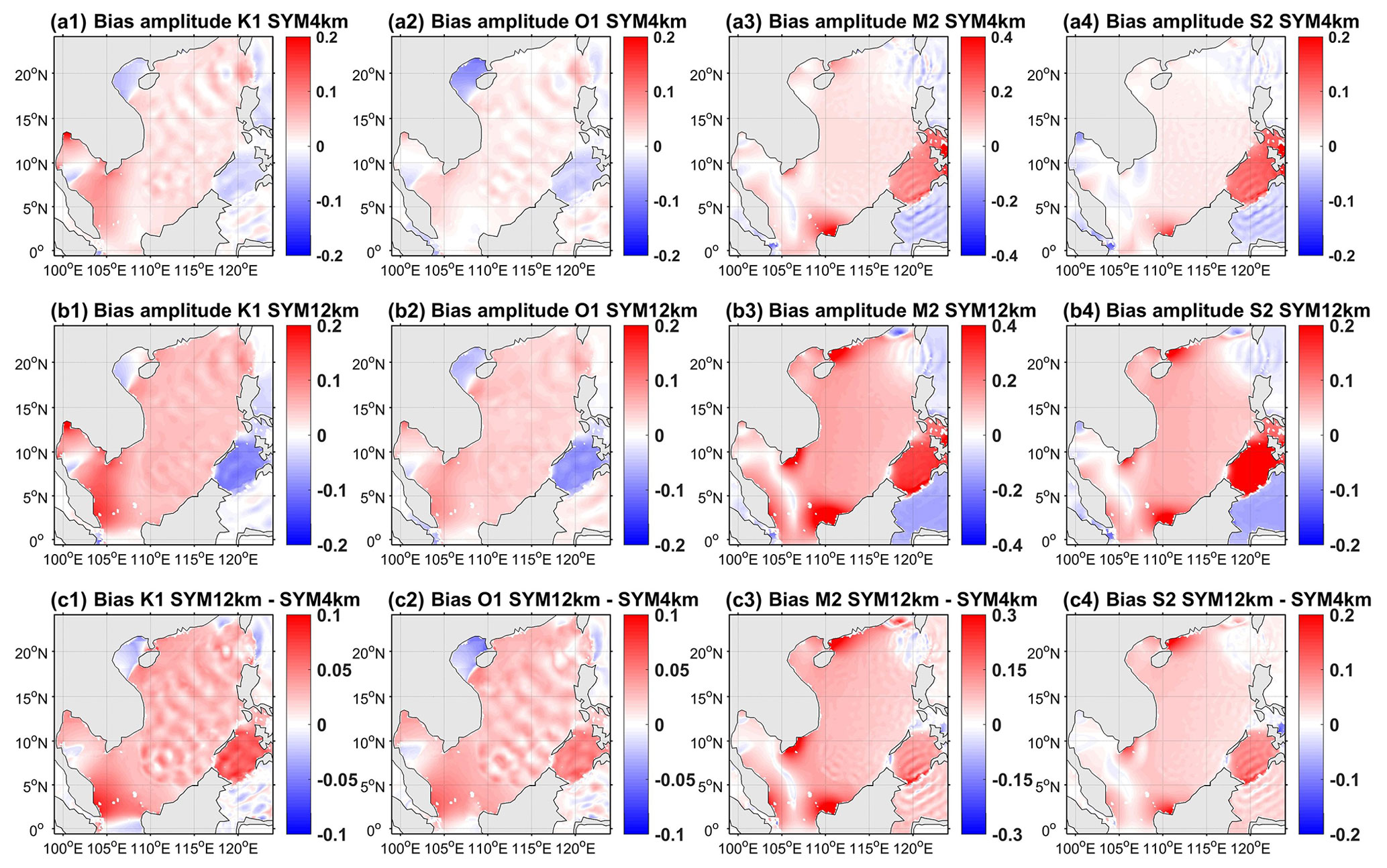
Figure A3 Bias of tidal amplitude (a1–a4) between SYM4 and FES2014 and (b1–b4) between SYM4 and FES2014 and (c1–c4)  the difference in absolute values of SYM12 and SYM4 biases for the following four tidal components: K1, O1, M2, and S2.

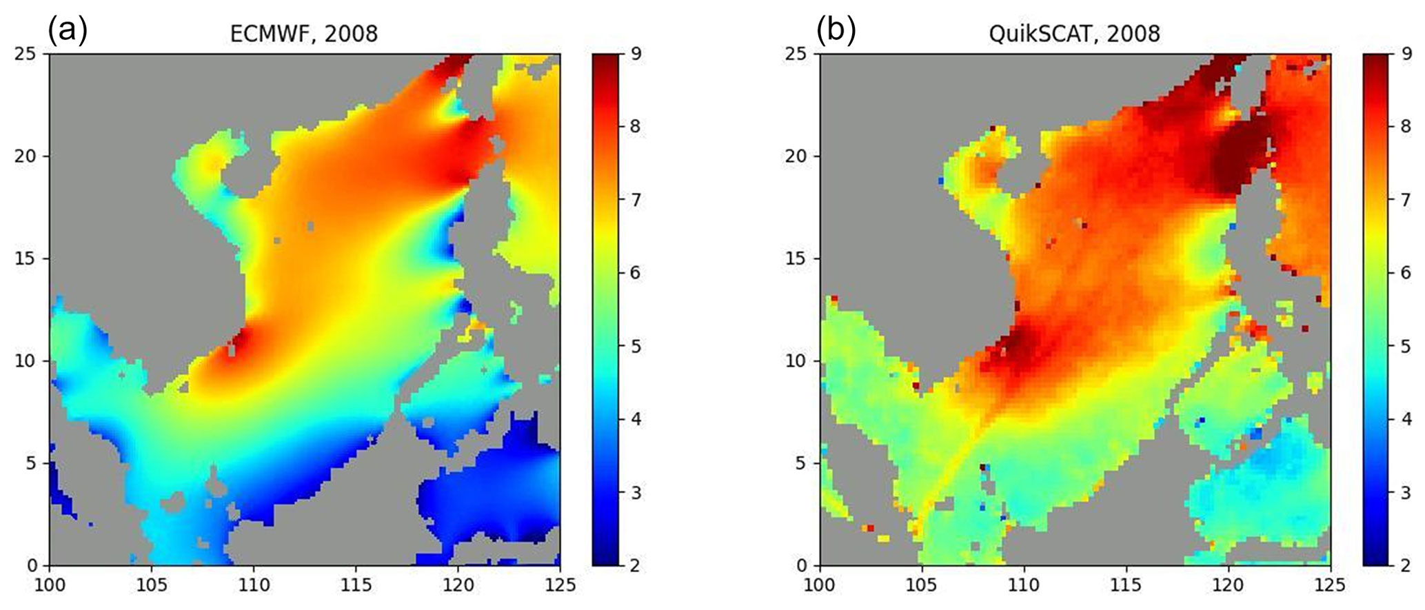
Figure A4 Sea surface wind speed (m s⁻¹) over the SCS averaged over the year 2008 computed from ECMWF 3 h analysis outputs (a) and daily QuikSCAT outputs (b).