Accounting for uncertainties in forecasting tropical-cyclone-induced compound flooding

Tropical-cyclone impacts can have devastating effects on the population, infrastructure, and natural habitats. However, predicting these impacts is difficult due to the inherent uncertainties in the storm track and intensity. In addition, due to computational constraints, both the relevant ocean physics and the uncertainties in meteorological forcing are only partly accounted for. This paper presents a new method, called the Tropical Cyclone Forecasting Framework (TC-FF), to probabilistically forecast compound flooding induced by tropical cyclones, considering uncertainties in track, forward speed, and wind speed and/or intensity. The open-source method accounts for all major relevant physical drivers, including tide, surge, and rainfall, and considers TC uncertainties through Gaussian error distributions and autoregressive techniques. The tool creates temporally and spatially varying wind fields to force a computationally efficient compound-flood model, allowing for the computation of probabilistic wind and flood hazard maps for any oceanic basin in the world as it does not require detailed information on the distribution of historical errors. A comparison of TC-FF and JTWC operational ensembles, both based on DeMaria et al. (2009), revealed minor differences of <10 %, suggesting that TC-FF can be employed as an alternative, for example, in data-scarce environments. The method was applied to Cyclone Idai in Mozambique. The underlying physical model showed reliable skill in terms of tidal propagation, reproducing the storm surge generation during landfall and flooding near the city of Beira (success index of 0.59). The method was successfully applied to forecasting the impact of Idai with different lead times. The case study analyzed needed at least 200 ensemble members to get reliable water levels and flood results 3 d before landfall (<1 % flood probability error and <20 cm sampling errors). Results showed the sensitivity of forecasting, especially with increasing lead times, highlighting the importance of accounting for cyclone variability in decision-making and risk management.

1 Introduction

Tropical-cyclone (TC)-induced compound flooding, which occurs when storm surge, heavy rainfall, high tides, and river discharge coincide, can have devastating impacts on coastal communities (Wahl et al., 2015). This type of flooding is particularly concerning as it can result in higher water levels and increased inland flooding, leading to damage and loss of life (e.g., Resio and Irish, 2015). The increased frequency and severity of compound-flooding events are expected to worsen due to climate change, including sea level rise (e.g., Easterling et al., 2000), changes in extreme storm surges and wave climates (e.g., Lin et al., 2012; Mori and Shimura, 2023), increased and prolonged precipitation (e.g., Trenberth et al., 2003), and ongoing coastal development and population growth (e.g. Neumann et al., 2015). Mitigation and preparedness strategies require a sound toolbox for assessing the impacts of TC-induced compound flooding on coastal communities to enhance short- to long-term decision-making.

Operational and strategic risk analyses are instrumental in analyzing and mitigating potential environmental risks. Operational risk analysis, typically associated with short-term forecasting (∼ several days), provides immediate response and preparedness for imminent disasters, ensuring the safety and protection of people and property (Roy and Kovordányi, 2012). Conversely, strategic risk analysis focuses on long-term climate variability assessments, delivering insights into hazards and their socio-economic and environmental impacts, thus facilitating informed policy decisions and adaptation strategies (e.g., Nederhoff et al., 2021). Though distinctly different, both perspectives are critical for comprehensive climate risk management as they offer different scales and time frames for prevention, preparedness, response, and recovery.

Forecasting agencies such as the National Hurricane Center (NHC) have significantly improved operational meteorological risk analysis, credited to gains made in numerical weather prediction models (McAdie and Lawrence, 2000; Cangialosi et al., 2020). Despite advancements, operational forecast errors remain significant enough to necessitate considering the inherent uncertainties in these forecasts for informed preparedness in decision-making (Lamers et al., 2023). A common probabilistic approach is to represent the resulting uncertainty in track prediction by means of a cone envelope as a graphical representation that illustrates the possible track variation of the TC center (NHC, 2023). The shape of the cone can be derived from the historical error data of the forecast and typically represents a 66.7 % probability that the track will be within the cone (i.e., 33.3 % chance the track falls outside the cone). The cone increases in size with lead time as the errors in the prediction accumulate. While the cone gives valuable insights into the potential range of TC variability of the core, it can be easily misinterpreted as the corresponding impacted area, which can be substantially larger. Quantification of the uncertainty in track prediction can be computed with several methods. For example, DeMaria et al. (2009) introduced a Monte Carlo method to generate 1000 realizations by randomly sampling from historical error distribution functions from the past 5 years for both the track and intensity. DeMaria et al. (2013) improved their method so that the track uncertainty is estimated on a case-by-case basis using the Goerss predicted consensus error (GPCE; Goerss, 2007), where the uncertainty is estimated based on the spread of a dynamical model ensemble instead of historical averages. Other methods exist – for example, Chen et al. (2023) introduced a deep-learning ensemble approach for predicting tropical-cyclone rapid intensification. However, these methods were all derived to provide insights, before landfall, into the uncertainty of the wind speeds and were not designed to force hydrodynamic or wave models and can thus result in too-erratic forcing conditions.

Early warning systems (EWSs) for coastal compound flooding are sensitive to uncertainties in the TC, including nonlinear interactions between the TC size, forward speed, location of landfall, tides, rainfall, and infiltration. However, often, EWSs for coastal flooding use physics-based and, due to computational constraints, deterministic approaches in which the best track is used to force a hydrological and hydrodynamic model that computes the storm surge and the complex interactions between coastal, fluvial, and pluvial processes. For example, the Global Storm Surge Information System (GLOSSIS) is based on Delft3D Flexible Mesh (Kernkamp et al., 2011) and runs operationally four times daily to produce 10 d water level and storm surge forecasts for the entire globe. GLOSSIS is typically forced with NOAA's GFS forcing, although there is also functionality in place to use hurricane tracks. Another example is the Coastal Emergency Risks Assessment (CERA) based on ADCIRC (Luettich et al., 1992). CERA is an effort to provide operational advisory services related to impending hurricanes in the United States only and uses the NHC official advisory every 6 h. Neither GLOSSIS nor CERA account for uncertainties in the meteorological forcing.

Several examples of probabilistic coastal flood methods do capture uncertainty in forcing. For example, the Global Flood Awareness System (GloFAS; Alfieri et al., 2013) is a modeling chain run by the European Centre for Medium-Range Weather Forecasts (ECMWF) based on the LISFLOOD hydrological model forced by 51 ensemble members. While GloFAS is an excellent resource for communities worldwide, it operates at a large scale with a relatively coarse resolution of 0.1° (∼ 10 km) and is thus not designed explicitly for TCs that require high spatial resolutions (Roberts et al., 2020) and does not account for relevant coastal processes such as tides. Higher resolutions and the inclusion of coastal processes can be found in several regional applications. For example, the Stevens Flood Advisory System (SFAS; Ayyad et al., 2022) is an ensemble-based probabilistic forecasting of tide, surge, and riverine flow across the US Mid-Atlantic and northeastern coastline and runs for 96 different atmospheric forcing datasets. Other examples include forecasting systems from the UK Met Office (Flowerdew et al., 2010) and the Royal Netherlands Meteorological Institute (de Vries, 2009). All these systems rely on coarser numerical forecasting products, focus on mid-latitude regions, and are thus not explicitly designed to forecast hazards related to TCs.

Probabilistic modeling systems for TC-induced coastal flooding for operational risk analyses in the US and Japan include P-Surge (Taylor and Glahn, 2008; Gonzalez and Taylor, 2018), which uses data from the NHC to create a set of synthetic storms by perturbing the storms' positions, sizes, and intensities based on past errors of the advisories. Subsequently, the Sea, Lake, and Overland Surge from Hurricanes model (SLOSH; Jelesnianski, 1992) is run and forecasts storm surge in real time when a hurricane is threatening. However, SLOSH does not account for several relevant (coastal) processes (e.g., tides, waves, rainfall, infiltration) and thus lacks their interactions. The Japan Meteorological Agency (JMA) does use a dynamic tide and storm surge model (Nakagawa, 2009), but this only accounts for a limited number of 11 ensemble members (Hasegawa et al., 2015). Moreover, both methods are created with a specific region in mind and are not easily transferable to other locations.

Besides probabilistic physics-based techniques, statistical machine learning techniques (e.g., Lecacheux et al., 2021, or Nguyen and Chen, 2020) are becoming increasingly popular for reducing the computational expense of forecasting compound flooding. However, these machine learning downscaling methods lack nonlinear interactions between relevant coastal processes driving compound flooding. Hybrid methods focus on reducing the number of tracks simulated and have proved to be capable of accurately representing a larger set of scenarios (Bakker et al., 2022).

As introduced by Suh et al. (2015), the constraints in real-time forecasting for operational risk analysis are around both accuracy and promptness. In other words, the time constraints associated with forecasting dictate that some modeling systems use a purely deterministic approach or a limited number of ensemble members to perform more detailed compound-flooding predictions and thus simplify the meteorological uncertainty (e.g., GLOSSIS, CERA, JMA). On the other hand, probabilistic approaches for meteorology with a large number of ensemble members use simplified hydrodynamics or have an insufficient resolution for TCs and thus do not account for the processes needed to forecast TC-induced coastal compound flooding (e.g., GloFAS, SFAS, NHC). In summary, the current shortcomings of existing methodologies include the lack of high-resolution models specifically tailored for analyzing coastal compound flooding. Additionally, there is a notable deficiency in probabilistic assessments of tropical-cyclone flooding that incorporate the uncertainties inherent in forecasting cyclone tracks. Moreover, there is a need for a universally applicable methodology that can be seamlessly adapted to various case studies globally.

To address the limitations listed, we propose a method to generate probabilistic wind and compound-flood hazard maps by using, for the first time, ensemble techniques via statistical emulation of TCs combined with physics-driven modeling for coastal compound flooding. The workflow emulates the TC evolution using an autoregressive technique in combination with reported mean errors in track and intensity, similarly to DeMaria et al. (2009) but without the need for historical error distribution functions. Next, this emulator produces an ensemble of several (herein thousands of) TC members. Then, for each ensemble member, a temporally and spatially varying wind field is generated and used to force a computationally efficient compound-flood model, SFINCS (Leijnse et al., 2021). The output consists of probabilistic wind and flood hazard maps that can be forecast on time with limited computational resources anywhere in the world. This paper refers to the TC forecasting framework as the Tropical Cyclone Forecasting Framework, TC-FF.

The paper is structured as follows. Section 2 introduces the Monte Carlo forecasting methodology. Section 3 describes the case study site and historical event of interest. The materials and methods used in this paper are described in Sect. 4. Validation in terms of tides and storms and application of the forecasting methodology are presented in Sect. 5. Finally, Sects. 6 and 7 discuss and summarize the main conclusions of the study.

2 Tropical Cyclone Forecasting Framework

In this paper, we introduce the probabilistic Tropical Cyclone Forecasting Framework, TC-FF, to compute TC-induced compound flooding for operational risk analysis. Our approach integrates a TC emulator using a Monte-Carlo-based ensemble sampling generation with an autoregressive technique, which is a simplified adaptation of DeMaria et al. (2009). The ensemble members are generated around the forecasted official track considering the average intensity, cross-track, and along-track historical errors. We deem these variables to be the primary source of track uncertainty (e.g., Fossell et al., 2017). Other variables (e.g., information on wind radii) can be (stochastically) correlated to them. The ensemble members are provided as input for the fast compound-flood model called SFINCS. Additionally, TC-FF considers tidal movements, storm surge, precipitation, and infiltration. The outcomes are consolidated into a unified probability product. By choice, each member has an equal likelihood of occurrence. The Python code for this method is accessible on GitHub via the following link: https://github.com/Deltares-research/cht_cyclones (last access: 26 December 2023​​​​​​​); otherwise, one is referred to Zenodo (Nederhoff and van Ormondt, 2023).

2.1 TC-FF flowchart

A compact flowchart of TC-FF used to generate the ensemble member is shown in Fig. 1. The steps of this process are as follows:

1. Define settings. The user specifies the data source, the period, the time step of the ensemble generation, and the number of ensemble members requested.

2. Input best track. The code either determines the best track based on gridded temporally and spatially varying wind and pressure fields (e.g., COAMPS-TC; Doyle et al., 2014) or reads the track forecasted by one of the forecasting centers (e.g., NHC or other agencies).

3. Along-track, cross-track, and intensity error matrices. The tool first computes random realizations based on the along-track, cross-track, and intensity standard deviations imposed for the time steps requested. The imposed mean absolute error is scaled with the time step to overcome any time step dependency.

4. Generate ensemble members. Following the approach of DeMaria et al. (2009), a Monte Carlo method generates numerous ensemble members based on error matrices of the previous step in combination with an autoregressive technique for the along-track, cross-track, and intensity errors.

5. Generate wind, pressure, and rain fields. Next, we generate meteorological forcing conditions, i.e., the surface wind and pressure fields per time step per ensemble member, based on parametric methods (e.g., Holland et al., 2010) for subsequent analysis and application within numerical models. Rainfall can be included as well via intensity relationships.

6. Simulation and post-processing. In this study, the compound-flood model SFINCS is applied, but in principle, other hydrodynamic models can also be applied, albeit typically at a higher computational expense. Data from the different ensembles are combined into several probabilistic outputs ranging from the probability of gale-force winds (wind speed >35 knots or >18 m s⁻¹) to compound flooding (water depth >15 cm) to quantile estimates (e.g., 1 % exceedance water level).

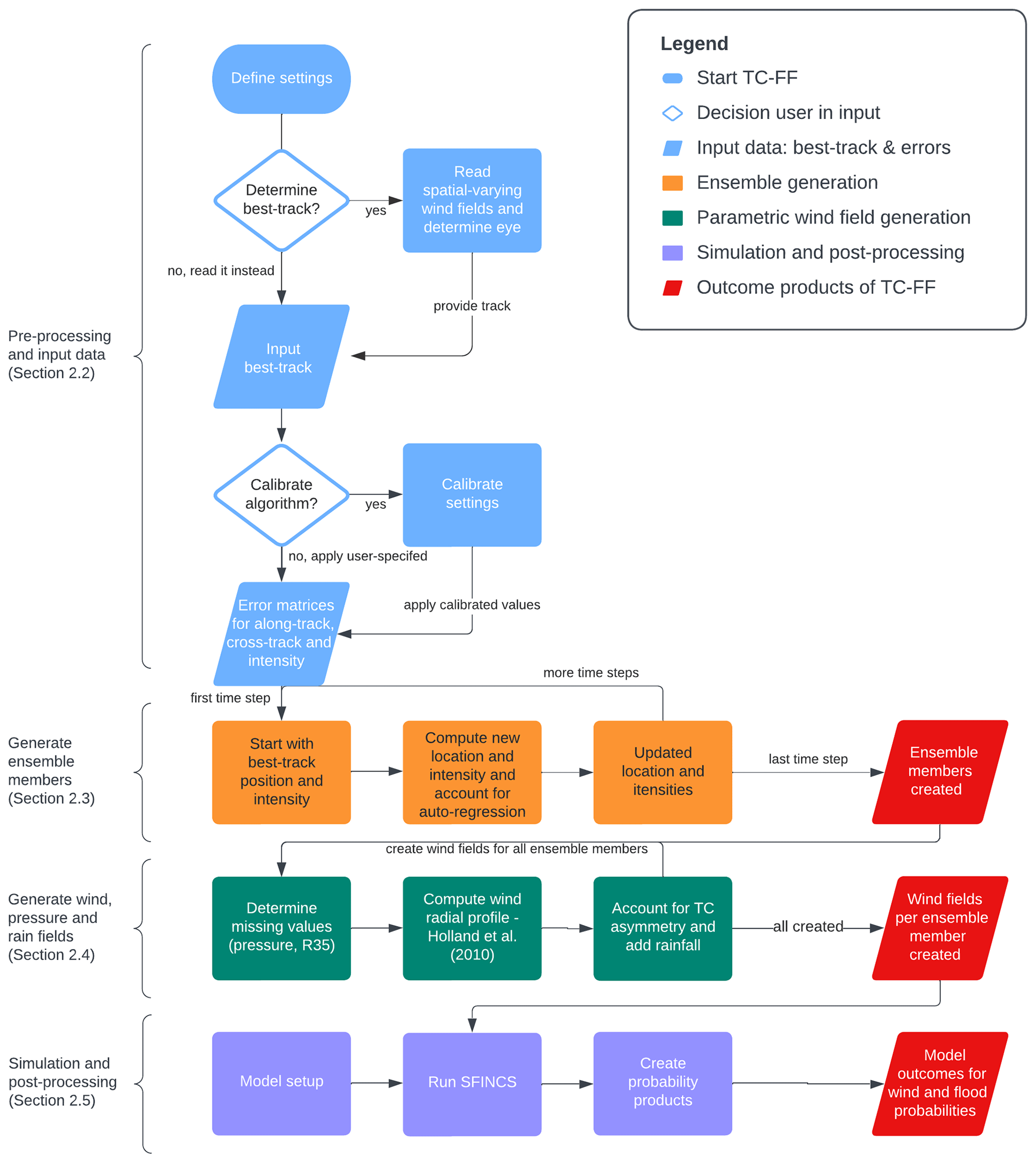
Figure 1 Flowchart of the Tropical Cyclone Forecasting Framework (TC-FF). Pre-processing stages are represented in light blue, the computational core of ensemble generation is denoted in orange, the parametric wind field generation is portrayed in green, the hydrodynamic simulation and analysis of winds are marked in purple, and the outcomes are marked in red.

In the subsequent paragraphs, we describe in more detail the pre-processing, the computation of the ensemble members (track and intensity variations), and the determination of temporally and spatially varying wind fields.

2.2 Pre-processing and input data

The pre-processing of TC-FF comprises three components

First, one specifies the period they would like to simulate, including the total time period over which wind fields need to be generated and the time period over which the ensembles need to be generated. In addition, a time step for ensemble generation (default 3 h) needs to be specified. At this stage, one also specifies the along-track, cross-track, and intensity mean absolute errors and auto-regression coefficients. When these values are unknown, calibration needs to be performed to determine them by comparing them with the reported errors of the forecast center (see calibration in Sect. 5.2.1). At this stage, one also specifies the number of ensemble members requested. The influence of the number of ensemble members is discussed in Sect. 5.3.2.

Second, since TC-FF creates random realizations around the best track, an input track is needed. Depending on the application, TC-FF reads a forecast bulletin that generates the track or determines the best track from the output of a high-resolution regional meteorological model. The determination of a track from a meteorological model is based on an algorithm that finds the minimum pressure in an area of interest. It takes in grid values, u and v wind components, pressure, and the minimum distance for clustering and returns lists of x and y coordinates of cyclone eyes, as well as the maximum wind speed and pressure around each eye.

Third, before the generation of the ensemble members, TC-FF creates random errors with a normal distribution based on the provided average errors. Matrices are two-dimensional, with one dimension being the number of time stamps and the other the number of ensemble members. The imposed mean absolute error is scaled with the time step to overcome any time step dependency and is then converted into a standard deviation.

2.3 Ensemble members

2.3.1 Track realizations and calibration

An important component in TC-FF is the generation of track realizations (or ensemble members) from the official track forecast. The official positions are interpolated with a spline function to include values at all requested times. Our approach for the track realization largely follows DeMaria et al. (2009). We decompose the track error into the along-track (AT) and cross-track (CT) components and account for the track error serial correlation via autoregressive regression (Eqs. 1 and 2).

$$\begin{array}{}\text{(1)}& {\displaystyle }{\mathrm{AT}}_t=a_t{\mathrm{AT}}_{t-i}+B_{\mathrm{rnd}}\text{(2)}& {\displaystyle }{\mathrm{CT}}_t=c_t{\mathrm{CT}}_{t-i}+D_{\mathrm{rnd}}\end{array}$$

In the above equations, AT_t and CT_t are the AT and CT errors at time steps t; a_t and c_t are constants; AT_t−3 and CT_t−3 are errors of the previous time step (typically i=3 h); and B and D are random numbers that are normally (Gaussian) distributed, scaled with the mean absolute error but limited to ±2σ.

Unlike DeMaria et al. (2009), we do not access the probability distributions of historical errors. Instead, we calibrate the parameters (a_t, c_t, and mean absolute errors for B and D) based on the reported historical errors from the agency responsible for the issued forecast (see Sect. 5.2.1). This is a simpler methodology and requires substantially fewer data (which is also typically not accessible outside the forecast centers). These historical errors are routinely reported by the forecast centers (e.g., see Sect. 4.1.2 for information on the data sources used in this paper). Note that errors in our implementation (both the error and the auto-regressive coefficient) do not vary with lead time. We calibrate a constant mean absolute error in combination with a single auto-regression coefficient (see Sect. 5.2.1 for calibration and Sect. 5.2.2 for the influence of simplifications). Moreover, the mean absolute error is converted into a standard deviation using a fixed relationship assuming a normal distribution of the error and scaled with the applied time step to allow the user flexibility in the applied time step.

The determination of the ensemble members is subsequently based on the sum of the forecast and random error components. In other words, we add the along-track and cross-track errors to the forecasted along- and cross-track. An example of the first 20 ensemble members is presented in Fig. 2b. Using this procedure, 10 000 ensembles are generated for each forecast case within this study; however, it is possible to use fewer ensemble members to reduce the computational cost but at larger statistical uncertainty (see Sect. 5.3.2 for trade-offs).

2.4 Intensity realizations and calibration

Similarly to the track realization, the maximum wind speed (intensity) at a specific interval is determined using a random-sampling approach. The starting point is the official forecast of intensity that is interpolated to include values at all requested times, and a random error component (VE_t) is added.

$$\begin{array}{}\text{(3)}& {\mathrm{VE}}_t=e_t{\mathrm{VT}}_{t-\mathrm{3}}+F_{\mathrm{rnd}}\end{array}$$

In the above equation, VE_t at time steps t and e_t is a constant; VE_t−3 refers to errors of the previous time step (typically 3 h); and F is random numbers that are normally distributed, scaled with the mean absolute error and limited to ±2σ.

The inland wind decay model adjusts the maximum intensity as a function of the distance inland, is directly based on DeMaria et al. (2009), and is computed with Eq. (4). If the intensity of any inland ensemble member exceeds this predetermined value at any forecast time, the intensity is adjusted to match this value. Subsequently, the intensity errors are recalculated based on the adjusted intensity. Additionally, if the intensity of an inland ensemble member falls to <7.7 m s⁻¹ (15 knots) at any point in time, the TC intensity is reset to zero for all subsequent periods to overcome any unrealistic re-intensifying TCs. All these criteria follow DeMaria et al. (2009).

$$\begin{array}{}\text{(4)}& V_i=\mathrm{20}+\mathrm{120}{e}^{\mathrm{0.0035}D}\end{array}$$

In the above equation, the maximum wind speed (V_i) in knots and the distance to land (D) in kilometers (with negative values indicating inland cyclones) are given, and the intensity of an inland cyclone can be determined.

The intensity implementation differs from DeMaria et al. (2009) in the following ways. We remove the dependency that the error scales with wind intensity and bias correction. Again, the determination of the ensemble members is based on the sum of the forecasted and random components computed with Gaussian mean absolute errors and an auto-regressive constant over lead time. Similarly to the track realization, intensity errors are scaled with the time step to overcome any time step dependency. The influence of the simplifications and the difference compared to NOAA operational code based on the original DeMaria et al. (2009) and DeMaria et al. (2013) implementations are discussed in Sect. 5.2.2.

2.5 Parametric wind fields

After the determination of the ensemble members, the temporally and spatially varying wind fields are constructed and written in a polar coordinate system. Several (horizontal) parametric wind profiles have been presented in the literature (e.g., Fujita, 1952; Chavas et al., 2015), with the original Holland wind profile (Holland, 1980) being the most widely used due to its relative simplicity. Several codes have been developed for storm surge models to provide temporal and spatial wind and pressure fields (e.g., Hu et al., 2012, for ADCIRC). Deltares has developed the Wind Enhance Scheme (WES; Deltares, 2018) to generate TC wind and pressure fields around the specified location of a tropical-cyclone center and given a number of TC parameters. In its current implementation, information on wind radii (radius of gale-force winds) can be considered in the Holland et al. (2010) formulation using information either from the best-track data or from the proposed relationships of Nederhoff et al. (2019), which increases the accuracy of the method. Furthermore, the asymmetry of the wind field in a TC is also implemented, as delineated by Schwerdt et al. (1979). Winds throughout this study are converted from 1 to 10 min using a conversion factor equal to 0.93 (Harper et al., 2010). Additionally, tropical-cyclone-induced precipitation can be incorporated using empirical relationships such as in the Interagency Performance Evaluation Task Force Rainfall Analysis (IPET, 2006).

2.6 SFINCS simulation and post-processing

After the determination of the wind fields for all the requested ensemble members, TC-FF runs a hydrodynamic model. In this study, we apply the compound-flood model SFINCS (Leijnse et al., 2021), which lends itself well to a large number of simulations in a reasonable amount of time due to its reduced complexity. SFINCS reads the tidal boundary conditions and wind, pressure, and rainfall conditions from the wind fields. Once all the ensemble member simulations have finished, probability products regarding wind and flood hazards are created. These products are created by sorting the results for each grid cell and providing estimates for either specific intervals (e.g., wind speeds >35 knots or water depth >15 cm) or quantile estimates (e.g., 1 % exceedance water level). Only track uncertainty is considered in these estimates.

3 Case study

The TC forecasting framework is applied to a historical event that took place in Mozambique's Sofala Province, Cyclone Idai, in March 2019. Mozambique is a country located in southeastern Africa (Fig. 2a). The country has a diverse population of over 31 million people, of which 2 million live in Sofala Province in central Mozambique. Sofala is primarily rural, with small communities along the Pungwe and Buzi river deltas (Emerton et al., 2020). Beira is the province's largest city, home to over 500 000 people, and is an important port linking the hinterland to the Indian Ocean. The city is prone to flooding, particularly during the rainy season, which generally extends from October to April or May. This period coincides with the cyclone season as cyclones often bring intense rainfall to the region. The vulnerability of Beira to flooding is exacerbated by factors such as climate change, rapid urbanization, and limited infrastructure.

Cyclone Idai was an example of a compound-flood event that affected large parts of the coastal delta of Sofala (Eilander et al., 2023). The storm began as a tropical depression in the Mozambique Channel, causing extensive flooding after its first landfall in early March. It later intensified as it moved back over the sea, developing into a tropical cyclone with 10 min sustained wind speeds of 165 km h⁻¹. Idai made landfall near the port city of Beira, bringing powerful winds and resulting storm surges and heavy rains that caused widespread flooding and destruction. Large areas were flooded, first around the coast and, a few days later, more inland in the Buzi and Pungwe floodplains. The total rainfall across the 5 d from 13 to 18 March ranged from 250 to 660 mm (NASA GPM, 2019). Over 112 000 houses were destroyed, and an estimated 1.85 million people were affected (UN OCHA, 2019).

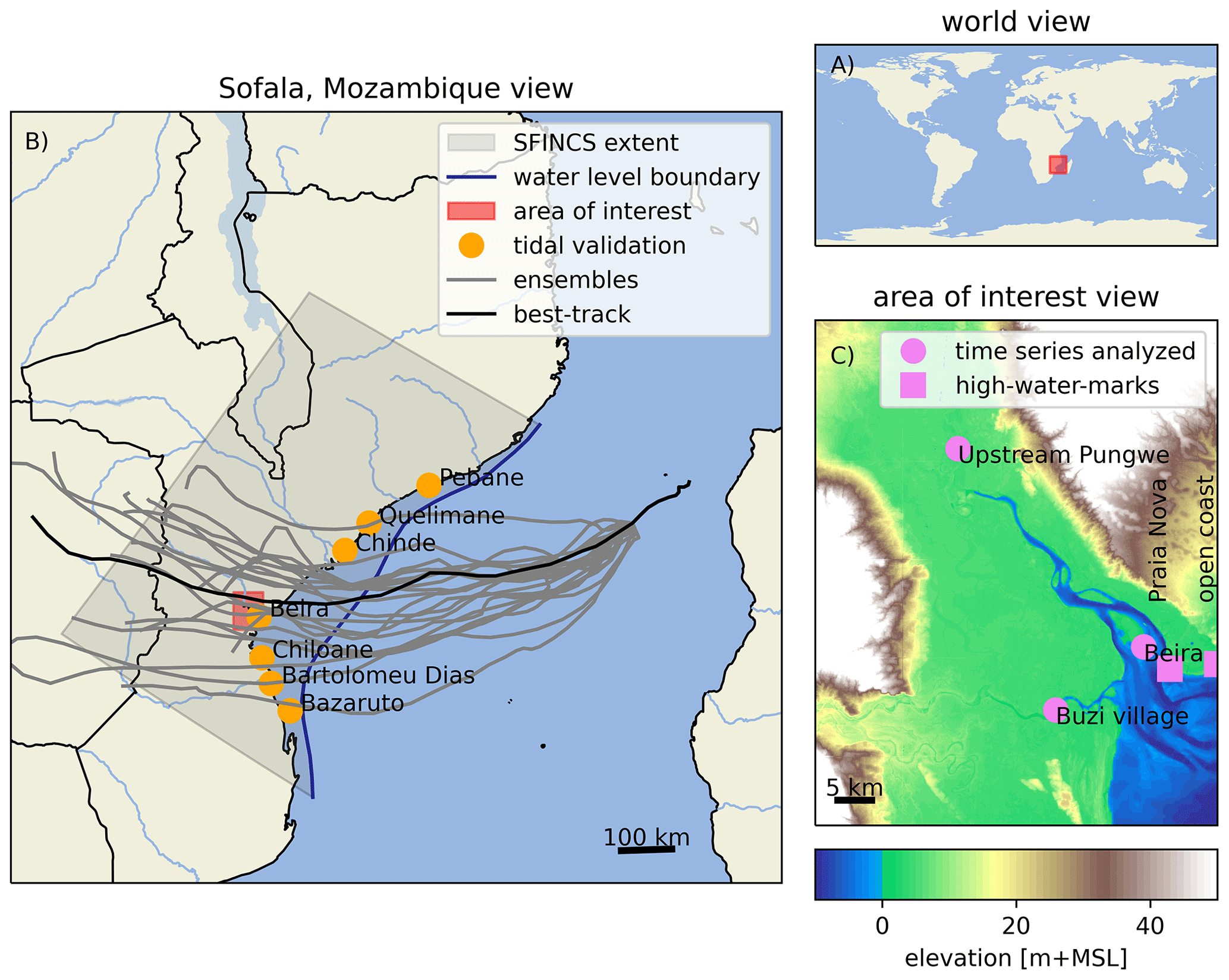
Figure 2 View of the study site: (a) Mozambique's Sofala Province is situated in the southeastern region of Africa in the Southern Hemisphere. (b) Geographical and hydrodynamic representation of the study area. The SFINCS model extent, highlighted in panel (b), encompasses a portion of the Sofala region, forced offshore with a water level boundary, and is validated at seven tidal stations (indicated by orange circles; see Appendix A). The best track is represented by a solid dark line, with the first 20 ensemble members 5 d before landfall demonstrated as gray lines. (c) The area of interest is the Pungwe estuary, situated near the city of Beira. Model validation also takes place at two high-water marks close to the city (signified by a purple box), with model outcomes depicted at three diverse locations across the estuary (marked by circles).

4 Material and methods

4.1 Materials

4.1.1 Elevation datasets

Several topographic and bathymetric datasets were collected and combined to develop a merged DEM. Data include field survey data points collected during three campaigns in November–December 2020 across Beira, locally collected lidar with a resolution of 2 m, bathymetric charts, MERIT (Yamazaki et al., 2017; 90 m), and GEBCO19 (International Hydrographic Organization and Intergovernmental Oceanographic Commission, 2003; 450 m). Careful consideration was given to prioritize specific datasets in space to ensure that the most detailed, recent, and accurate datasets were used in a given area. For example, survey and lidar data are prioritized over the usage of MERIT and GEBCO19. The merged DEM was produced based on a medium-resolution (50 m) regional DEM and a fine-resolution (5 m) local DEM in Beira. For more information on merging the data, one is referred to Deltares (2021).

4.1.2 Forcing conditions

Tidal boundary conditions were based on harmonic constituents provided by TPXO 8.0 (Egbert and Erofeeva, 2002), and tidal amplitudes and phases for all 13 available components were applied. The best-track data (BTD) by the Joint Typhoon Warning Center (JTWC) are used throughout this study for meteorological forcing conditions (JTWC, 2022). Reported error statistics by the JTWC for the 5-year average from 2016 to 2020 were used to inform the ensemble generation (JTWC, 2021). Ensemble members from TC-FF were compared to 1000 members produced with the code from NOAA, NHC, and JTWC based on DeMaria et al. (2009) and DeMaria et al. (2013), which is used operationally (Buck Sampson, personal communication, 5 June 2023).

4.1.3 Validation data

Observed tidal coefficients near the city of Beira were used for the calibration and validation of the model (van Ormondt et al., 2020; see Fig. 2 for locations). The validation of the event Cyclone Idai (2019) consisted of comparing both the observed and modeled flood extents in deltas of the Pungwe and Buzi rivers and high-water marks in the city of Beira. The observed flood extent was derived from Sentinel-1 synthetic aperture radar data (Eilander et al., 2023), and two observed high-water marks (Deltares, 2021) were used, one at Praia Nova, on the western side of the city, and another one at the open-coast beach in the southeast (see Fig. 2 for locations). Correspondingly, values of modeled flood extent and high-water marks were output at the same locations.

4.2 Methods

4.2.1 Area schematization

For this study, we employed the Super-Fast INundation of CoastS (SFINCS) model, which solves the simplified equations of mass and momentum for overland flow in two dimensions (Leijnse et al., 2021). The goal was to create one continuous compound-flood area model that computes tidal propagation, storm surge, and pluvial and fluvial flooding.

The area schematization builds upon Eilander et al. (2023) but varied in three ways. First, we extended the model alongshore and in deeper water to alleviate the need to nest it in a large-scale regional coastal circulation model and to generate tidal propagation and storm surge within the domain. The model was extended ∼ 500 km alongshore from Beira to ensure that a cyclone hitting Beira is fully resolved within the domain. Moreover, the model was extended to 1000 m water depth, where wind shear has a negligible impact on the storm surge. Using a quadtree implementation (e.g., Liang et al., 2008), we applied a variable model resolution ranging from 8000 to 500 m. A quadtree is a technique in which the refinement from one level to another is based on the original cell but divided into four smaller cells with a 2-times-smaller grid size, and it allows the extension of the model setup into deeper water without having time step restrictions in deeper water based on the explicit numerical scheme of SFINCS. Second, high-resolution topo-bathymetry and land roughness were included in the native resolution utilizing subgrid lookup tables (Leijnse et al., 2021). However, the hydrodynamic computations were performed on a coarser resolution to save computational time. DEM information up to 10 m was included in the 500 m grid cells (i.e., factor-50 refinement). Lastly, subgrid bathymetry features were included to account for maximum dune height based on the DEM to control overflow during storm conditions around Beira. For both the subgrid lookup tables and features, the elevation datasets from Deltares (2021) at 5 m resolution were used (see Sect. 4.1.1 for more information). For the lookup tables, we linearly interpolated the high-resolution DEM onto the subgrid. For the subgrid features, the line element had a resolution of 500 m per vertex, and the highest point in a radius of 500 m was used.

Spatially varying roughness and infiltration were used based on land elevation. All points above mean sea level (a.m.s.l.) have a high Manning friction coefficient of 0.06 s m${}^{-\mathrm{1}/\mathrm{3}}$ and an infiltration rate of 1.9 mm h⁻¹ (typical values from HSGs Group C; United States Department of Agriculture, 2009), and all other points have a lower friction of 0.02 s m${}^{-\mathrm{1}/\mathrm{3}}$ to represent water and do not have any infiltration. The SFINCS model was forced with tidal boundary conditions and temporally and spatially varying wind, pressure, and rainfall fields. At the offshore boundary, tidal water levels were imposed, and the inverted barometer effect was accounted for. We refer to Appendix A for the calibration of the tides, in which we show that the area model reproduces tides with a median mean absolute error (MAE) of 21 cm. Wind and pressure fields were created with the Holland wind profile (Holland et al., 2010) based on the BTD (see Sect. 2.4 for details). Rainfall for TCs was based on the Interagency Performance Evaluation Task Force Rainfall Analysis (IPET, 2006) method. Comparison with the reported rainfall total revealed a significant underestimation of cumulative rainfall during Idai based on IPET. Based on the magnitude of the underestimation, rainfall estimates by IPET were tripled, resulting in a cumulative rainfall in the area of interest of 495 mm for the best track, which is on a similar order of magnitude to observed rainfall (see Sect. 3). For fluvial processes, rather than using data sources like river discharge measurements or a hydrological model, our model only relies on a rain-on-grid with infiltration methodology to simulate surface runoff and its subsequent accumulation, thus providing a first-order estimate of fluvial flooding.

4.2.2 Simulations periods

The validation of the area schematization focused on two time periods. First, three spring-neap cycles (13 January until 26 February 2022) were used for the tidal calibration and validation in the area of interest (see Appendix A). Second, Idai was hindcasted, forced with the JTWC BTD, and compared to observational data for flood extent and high-water levels (Sect. 5.1). After validation of the area schematization, the new forecasting methodology introduced in Sect. 2 was applied. Various lead times ranging from 1 to 5 d before the second landfall for 10 000 ensemble members were computed (Sect. 5.3).

Model runs were performed on the Deltares Netherlands Linux-based High-Performance Computing platform using 10 Intel Xeon CPU E3-1276 v3 processors. The simulations were run on a CPU with openMP enabled to utilize the four cores per Xeon processor. On average, a 7 d Idai simulation took about 4 min on a single processor. Running all 50 000 events took ∼ 15 d using all 10 processors (or 40 cores).

4.2.3 Model skill

Several accuracy metrics were calculated throughout this study: model bias, mean absolute error (MAE; Eq. 5), root-mean-square error (RMSE; Eq. 6), and unbiased RMSE (uRMSE; RMSE with bias removed from the predicted value). These error metrics are used for the comparison of water levels, wind speed, and track errors.

$$\begin{array}{}\text{(5)}& {\displaystyle }\mathrm{MAE}={\displaystyle \frac{\mathrm{1}}{N}}\sum _{}^{}\left(\left|y_i-x_i\right|\right)\text{(6)}& {\displaystyle }\mathrm{RMSE}={\sqrt{{\displaystyle \frac{\mathrm{1}}{N}}\sum _{}^{}(y_i-x_i)}}^{\mathrm{2}}\end{array}$$

In the above equations, N is the number of data points, y_i is the ith prediction (modeled) value, and x_i is the ith measurement.

Moreover, skill is quantified by binary flood metrics (Wing et al., 2017). The model output (M) is converted to one of two states, wet (1) or dry (0), using a commonly used threshold of 15 cm (e.g., Wing et al., 2017) and compared to the Sentinel benchmark data (B). The critical success index (C; Eq. 7) accounts for both overprediction and underprediction and can range from 0 (no match between modeled and benchmark data) to 1 (perfect match between modeled and benchmark data).

$$\begin{array}{}\text{(7)}& C={\displaystyle \frac{M_{\mathrm{1}}{B}_{\mathrm{1}}}{M_{\mathrm{1}}{B}_{\mathrm{1}}+M_{\mathrm{0}}{B}_{\mathrm{1}}+M_{\mathrm{1}}{B}_{\mathrm{0}}}}\end{array}$$

For the comparison of cross-track, along-track, and intensity cumulative distribution functions (CDFs), we also applied the continuous ranked probability score (CRPS; Matheson and Winkler, 1976). CRPS measures how good forecasts are at matching observed outcomes; where CRPS = 0, the forecast is wholly accurate, and where CRPS = 1, the forecast is wholly inaccurate.

$$\begin{array}{}\text{(8)}& \mathrm{CRPS}\left(F,x\right)={\int }_{-\mathrm{\infty }}^{\mathrm{\infty }}{\left[F\left(y\right)-F_{\mathrm{0}}\left(y\right)\right]}^{\mathrm{2}}\mathrm{d}y\end{array}$$

In the above equation, F(y) is the CDF is associated with an empirical probabilistic reference and prediction.

4.3 Analysis method

The analysis of forecasting results was undertaken using several methods. Initially, extreme wind speeds and water levels were assessed by charting them as time series data, inclusive of quantile estimates such as the 95 % confidence interval (CI). Following this, the maximum values registered during the simulation were organized into cumulative distribution functions (CDFs). This process offered insights into their exceedance probability. Finally, the mean probability of flooding was computed. The method to derive this value entailed counting the instances where computational cells registered a minimum of 15 cm of water. Only cells positioned above mean sea level (a.m.s.l.) were incorporated into the area estimates.

5 Results

This section is organized into three parts, each addressing a crucial aspect of our study on Cyclone Idai's compound flooding. First, we assess the model's accuracy in simulating tidal, storm surge, and combined pluvial and fluvial impacts (Sect. 5.1). Next, calibration of TC-FF in relation to along-track, cross-track, and intensity average errors for the Southern Hemisphere and validation of TC-FF for Idai, specifically in relation to the implementation from NOAA, NHC, and JTWC, which are used operationally, are presented (Sect. 5.2). Lastly, we delve into forecasting uncertainties and their effects on flood predictions using ensemble simulations with various lead times (Sect. 5.3).

5.1 Verification of the numerical model for Cyclone Idai

Computed water levels near Beira show the strong tidal modulation and the wind-induced storm surge during the landfall of the cyclone (Fig. 3 – panel a, blue line for water level and vertical line for moment of landfall). Based on the difference between the predicted astronomic tide and the total modeled water level, we estimate a storm surge of >3.5 m due to the ∼ 45 m s⁻¹ wind speeds (Fig. 3 – panel b). The storm surge at Beira is driven by wind setup, as well as by pluvial and fluvial drivers. Deeper in the estuary, in the Pungwe floodplains, water levels peaked several days after landfall due to intense upstream rainfall and subsequent runoff. Water levels near Buzi Village seem to be a combined result of, first, marine and, second, riverine-driven water levels.

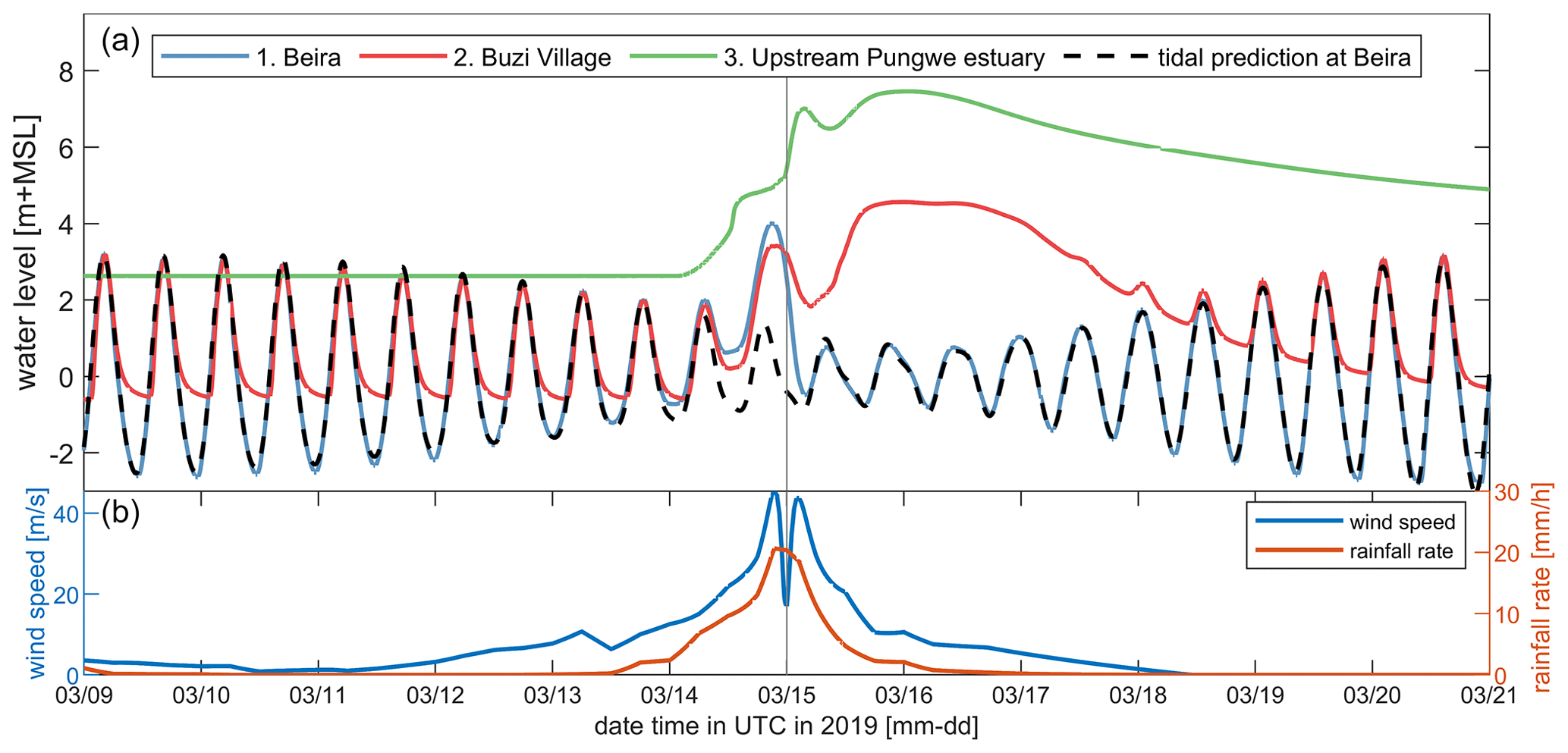
Figure 3 Time series of water levels, wind speed, and precipitation within the study area. (a) Computed water levels at various locations (blue for Beira, red for Buzi Village, and green for upstream in the Pungwe estuary (see Fig. 2c for their location), with the dashed black line representing the astronomical prediction at Beira). (b) Simulated wind speed (blue) and rainfall rate (red) over the same period. Idai made landfall on 15 March, and its powerful winds and rainfall resulted in marine flooding at Beira and riverine-driven flooding upstream in the estuary. The vertical line represents the moment of landfall.

Validation of the SFINCS model for the observed extent (blue colors in Fig. 4a) gives confidence in the ability to simulate the compound flooding (Fig. 4). The model can reproduce the Sentinel-1-derived extent with a critical success index of 0.59. This skill score is comparable to previous work by Eilander et al. (2023), though it is somewhat lower. Based on the differences between the modeled and satellite-derived extents, it becomes apparent that the model underestimates the flooding around the Buzi River (false negative; orange colors in Fig. 4b around 660–7800 km). We hypothesize this is due to the lack of river inflow related to an underestimation of rainfall further upstream and/or an overestimation of infiltration due to soil saturation which is not considered. Moreover, the comparison with satellite-derived flood extent indicates an overestimation of the flooding at Beira (false positive; red colors in Fig. 4). Here, we suspect that the benchmark data might be off and that the coastal flooding already receded before the Sentinel data recorded the extent. The observed high-water marks near Beira ranged from 3.6 m within the estuary to 2.9 m a.m.s.l. at the open coast and are reproduced by SFINCS at, respectively, 3.8 and 3 m a.m.s.l. This difference suggests a positive bias of the model results at the coast of ∼ 10–20 cm, similarly to the tidal validation (see Appendix A), which revealed a median MAE of 21 cm.

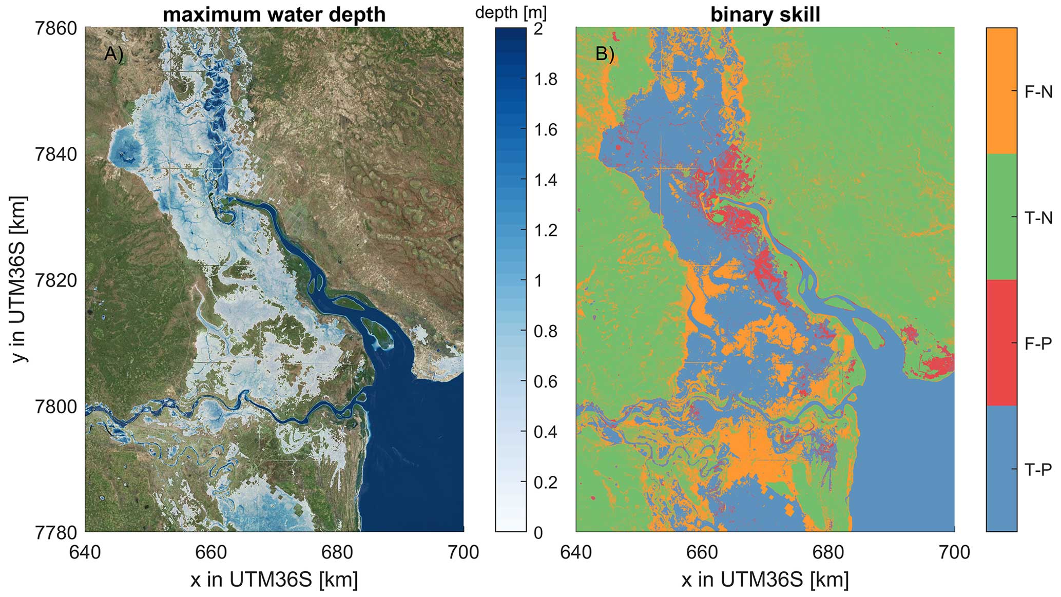
Figure 4 Maximum computed water depth (panel a) and binary skill of flood extents for Idai (panel b). Water depths are downscaled from the model resolution to the 10 × 10 m resolution of the topo-bathymetry. The binary skill evaluation (panel b) assists in determining the model's accuracy and dependability, and the Sentinel-1 radar data are used as a reference to determine skill. A true-positive (T-P) outcome denotes a correct flood prediction by the model compared to Sentinel-1-derived extent, whereas a false-positive (F-P) outcome occurs when the model forecasts a non-existent flood. In contrast, a false-negative (F-N) outcome indicates where the model overlooks an actual flood, and a true-negative (T-N) result occurs when the model accurately predicts the lack of a flood event. The model produces large-scale flooding, which is largely also observed in the data, but local differences in terms of over- and underestimation exist. The coordinate system of this figure is WGS 84/UTM 36 S (EPSG 32736). © Microsoft.

5.2 Calibration and influence of simplifications of TC-FF

5.2.1 Calibration of TC-FF: mean absolute error and auto-regression

This study used JTWC-reported errors for the along-track, cross-track, and intensity of the Southern Hemisphere to calibrate our methodology (JTWC, 2021). For other case studies (for example, based on different forecasting agencies or in other ocean basics), these reported errors can be used instead. Calibration is performed by minimizing the square-root difference between computed and reported mean absolute values for various lead times using the Nelder–Mead method. This effort resulted in mean absolute errors for B and D of 68.5 and 55.3 km and auto-regression coefficients a_t ad c_t of 1.214 and 1.181 (Fig. 5a and b) for the along-track and cross-track. Moreover, we calibrated the mean absolute error and regression coefficients for the intensity, which resulted in a mean absolute error for F of 9.28 m s⁻¹ and an auto-regression coefficient e_t of 0.624 (Fig. 5c).

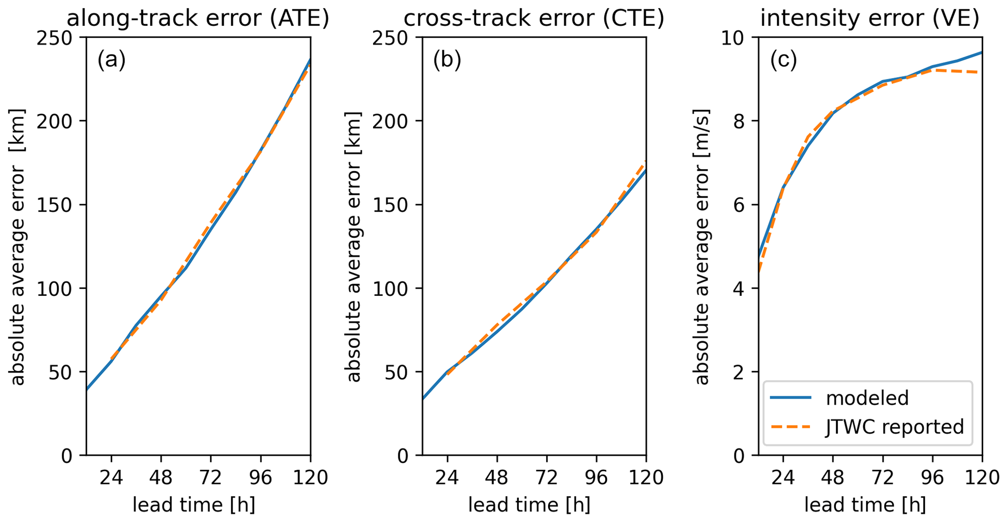
Figure 5 Comparison of calibration results for the probabilistic forecasting method TC-FF (solid blue line) and the Joint Typhoon Warning Center (JTWC)-reported error statistics based on the 5-year average (2016–2020) in the Southern Hemisphere (dashed orange line). Panel (a) represents the along-track error, panel (b) demonstrates the cross-track error, and panel (c) exhibits the wind speed or intensity error. Modeled errors are based on 1000 ensemble members. Modeled absolute average errors are similar to JTWC.

5.2.2 Comparison of TC-FF with operational forecast products

Errors produced by TC-FF are compared to the implementations from NOAA, NHC, and JTWC that are used operationally. Minor differences between the TC-FF and full implementation based on DeMaria et al. (2009) and DeMaria et al. (2013) exist and are attributed to the simplifications used in the error distribution (including the lack of GPCE). The distribution of along-track, cross-track, and intensity errors is typically in the same order (Fig. 6), which is confirmed by median CPRSs over various lead times from 0 to 120 h of 0.07, 0.05, and 0.10 and median MAEs of 37 km, 21 km, and 7 m s⁻¹ for, respectively, the along-track, cross-track, and intensity. At the same time, TC-FF has, by design, no bias corrections in terms of cross-track, along-track, and intensity errors, whereas the operational system does, leading to the positive median along-track error in red compared to the blue line in Fig. 6a and a median bias of −16 km. Besides the median estimates, the interquartile range (25 %–75 %) and 95 % CI match relatively well for the along-track and cross-track errors. Larger differences are found for the intensity error. In general, the wind intensity error looks visually erratic and does not start at zero for no lead time, which is the result of the inland wind decay model. Both JTWC and TC-FF have a negative bias due to the effect of land, but TC-FF does have a median bias of +6.7 m s⁻¹ compared to JTWC, suggesting that TC-FF overestimates. However, more substantial differences are found for the interquartile range and 95 % CI. These findings for the along-track, cross-track, and intensity are supported by a more detailed analysis of the CDF for the different parameters as a function of lead time (see Figs. B1, B2, and B3 in Appendix B). For the along-track and cross-track, we observe an increase in the MAE and uRMSE as a function of lead time but a decrease in the CPRS. The increasingly larger error distribution influences this pattern. Moreover, TC-FF produces Gaussian distributed errors, while the JTWC error distribution differs since it is based on historical error distributions and is adjusted based on the GPCE. Similarly to Fig. 6, larger differences are found for the intensity error, which is influenced by the bias correction that increases with lead times.

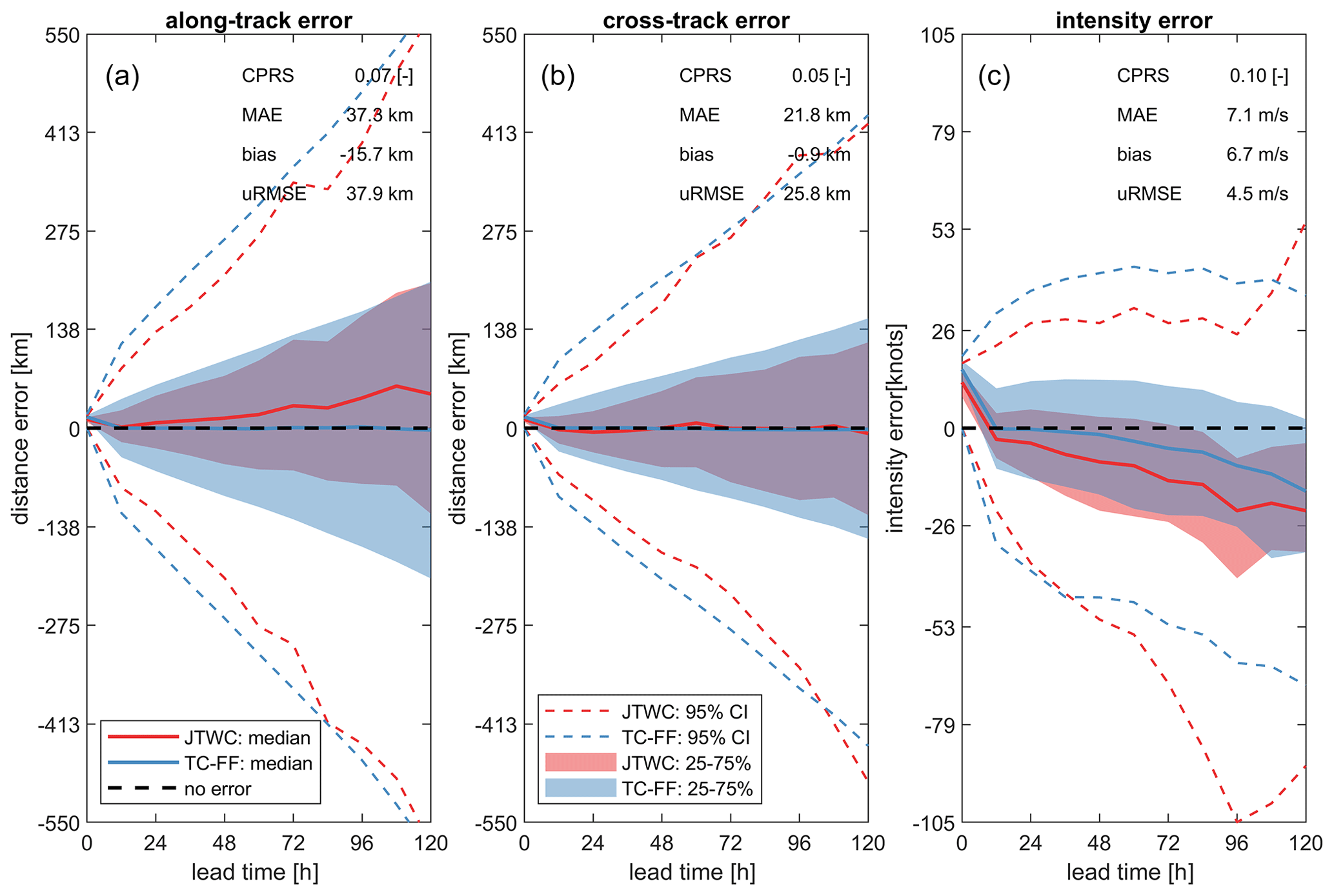
Figure 6 Comparison of validation results for the probabilistic forecasting method TC-FF (blue line) and the Joint Typhoon Warning Center (JTWC) operational product (red line). Panel (a) represents the along-track error, panel (b) demonstrates the cross-track error, and panel (c) exhibits the wind speed or intensity error. Errors are computed for both the TC-FF and JTWC based on 1000 ensemble members. Solid lines are median estimates, shaded areas are the interquantile range (25 %–75 % CI), and the dashed line is the 95 % CI. TC-FF and JTWC produce broadly similar error distributions for different lead times.

5.3 Forecasting of Idai using the TC-FF

This section presents the application of forecasting Idai using the TC-FF.

5.3.1 Uncertainty 3 d before landfall

The TC-FF method with 10 000 ensemble members is applied to the case of Cyclone Idai. The results reveal that accounting for the uncertainty of the TC track and the intensity of the eye 3 d before landfall results in considerable uncertainty regarding wind speeds and water levels near Beira (Fig. 7) or the region (Fig. 8). In particular, the wind speeds show a 95 % CI of about 7–40 m s⁻¹ at the moment of landfall (Fig. 7a) versus ∼ 45 m s⁻¹ or a Saffir–Simpson hurricane wind scale (SSHWS) of 2 in terms of the best track. Moreover, TC category-1 wind speeds could occur as early as 14 March at 07:30 UTC or as late as 15 March at 11:10 UTC. This spread of possible maximum wind speeds in Beira results from the large uncertainties in intensity and a difference in landfall location and time. Based on the same model simulations, the empirical cumulative distribution function (CDF) of the maximum wind speed at Beira ranges from 8.8 to 59.2, with a median wind speed of 25.5 m s⁻¹, while the best track has a 5.9 % exceedance probability (Fig. 7b). Consequently, water levels vary greatly (Fig. 7c). For example, ensemble members can exhibit a sizable wind-driven setup due to TC wind blowing from offshore into the estuary, pushing water up in the estuary and in Beira. For landfall locations west of the estuary, the wind blows offshore, resulting in a large set-down. Note that Beira is in the Southern Hemisphere, and due to the Coriolis effect, TCs spin clockwise. The highest water levels occur when high tides and wind-driven setups coincide, which explains the three peaks in the 95 % CI water level given the semi-diurnal tide and the highest possible wind speed for ∼ 1.5 d (Fig. 7c). The maximum water levels are dominated by the tide except in the situation of cyclone impact (see the CDF in Fig. 7d and the minimum value of ∼ 3.5 m a.m.s.l. around 90 %, which is influenced by the tide and time window over which it is determined). The specific track of Idai resulted in relatively extreme conditions compared to other possible combinations (both for winds and water levels). A similar pattern can be observed in the spatial maps shown in Fig. 8. The average probability of flooding in the area is 26 %, with higher probabilities of flooding found in the lower-lying portions of the estuary (note that we are excluding points below mean sea level (m.s.l.); Fig. 8a). The 1 % exceedance flood depth threshold shows a large extent and is quite similar to the computed extent due to Idai (see Fig. 4a for comparison with Fig. 8b). The main difference is that there is more flooding near the city of Beira and somewhat less near Buzi Village. The match between the 1 % exceedance flood depth and the best track with Idai suggests that the event was relatively severe and implies that, even though many other potential scenarios could have unfolded, they likely would not have resulted in the same extensive flooding caused by Idai.

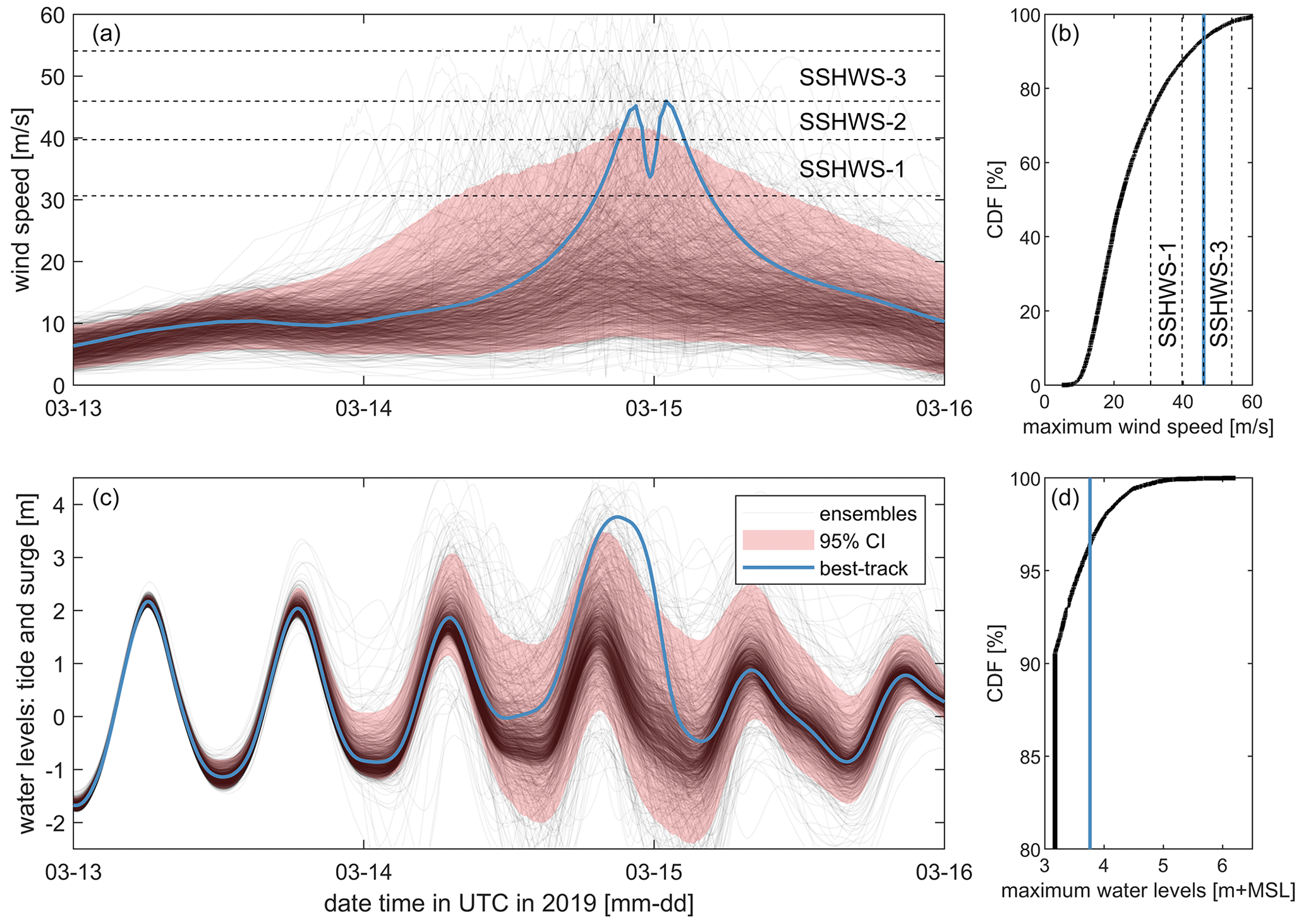
Figure 7 Multi-panel analysis of wind and water levels 3 d before landfall: (a) time series of wind speeds, (b) maximum wind speeds, (c) time series of water levels near Beira, and (d) maximum water levels. Data are derived from 10 000 ensemble members (transparent black line; every 10th plotted), with red shading representing the 95 % CI. The best track (blue line) and the Saffir–Simpson hurricane wind scale are included for comparison (panels a and b only). There is substantial uncertainty in wind speeds and water levels near Beira 3 d prior to landfall.

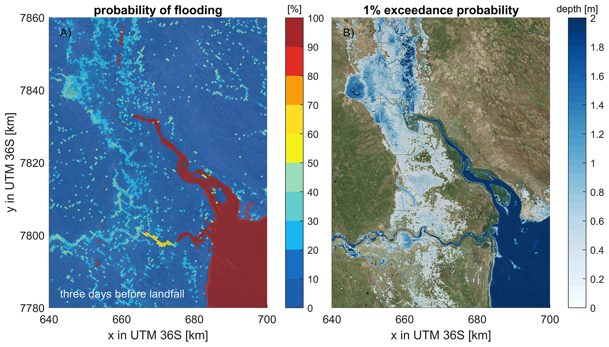
Figure 8 Probabilistic flood analysis for Cyclone Idai 3 d before landfall: (a) spatial distribution of flooding probability and (b) corresponding 1 % exceedance water depth estimates, highlighting areas of most significant hazard. Results in panel (a) are determined from 10 000 ensemble members based on the original 500 m model resolution, while water depth in panel (b) is downscaled to the original 10 × 10 m bathymetry resolution. Higher probabilities of flooding are found in the lower-lying portions of the estuary. The coordinate system of this figure is WGS 84/UTM 36 S (EPSG 32736). © Microsoft.

5.3.2 Influence of sampling size

As described by Cashwell and Everett (1959) and DeMaria et al. (2009), the precision of Monte Carlo techniques is proportional to the number of ensemble members (N). The convergence rate typically shows a slower progression than $\mathrm{1}/N$, constituting a limitation intrinsic to all Monte Carlo methods. To investigate the convergence rate and the error induced by employing a finite number of ensemble members, the Idai forecasting case 3 d prior to landfall is used, analogously to the preceding section, albeit with a variable number of ensemble members. Additionally, bootstrapping is employed to approximate convergence rates and the accompanying uncertainty.

The estimation of the 95 % exceedance maximum water levels in proximity to Beira exhibits convergence with the number of ensemble members, albeit with considerable deviations compared to a fully converged solution with 10 000 members when implementing a low number of ensemble members (Fig. 9a). For instance, employing merely 50 ensemble members results in an interquartile range (25 %–75 %) of −0.28 to +0.10 m. Increasing the number of ensemble members reduces this sampling uncertainty to a range of −0.09 to +0.06 m for 200 ensemble members.

Similarly, the standard deviation for several quantiles of maximum-water-level estimates at Beira is reduced with more ensemble members. It exhibits a similar pattern from higher to lower quantiles (Fig. 9b). In essence, estimating rare events necessitates executing more ensemble members to attain comparable convergence. This study found that the 95 % exceedance maximum water level at Beira when utilizing 200 ensemble members has a standard deviation of 21 cm (blue line Fig. 9b). This level of convergence seems acceptable since it is of a similar order to the skill of the hydrodynamic model (see Sect. 5.1).

The probability of error in flood potential is expressed as a function of N on a log–log plot (Fig. 9c). Compared to a fully converged solution with 10 000 members, for N=200, the mean error constitutes 0.95 %, and the maximum error amounts to 1.53 %. Note that this estimate is without considering the model error. In the log–log diagram, the errors exhibit near-linear correlations with N and could serve as a basis for determining the number of ensemble members needed for a specified confidence level. For instance, to achieve a maximum error of 1 % in flood probability, it would be necessary to utilize 500 ensemble members.

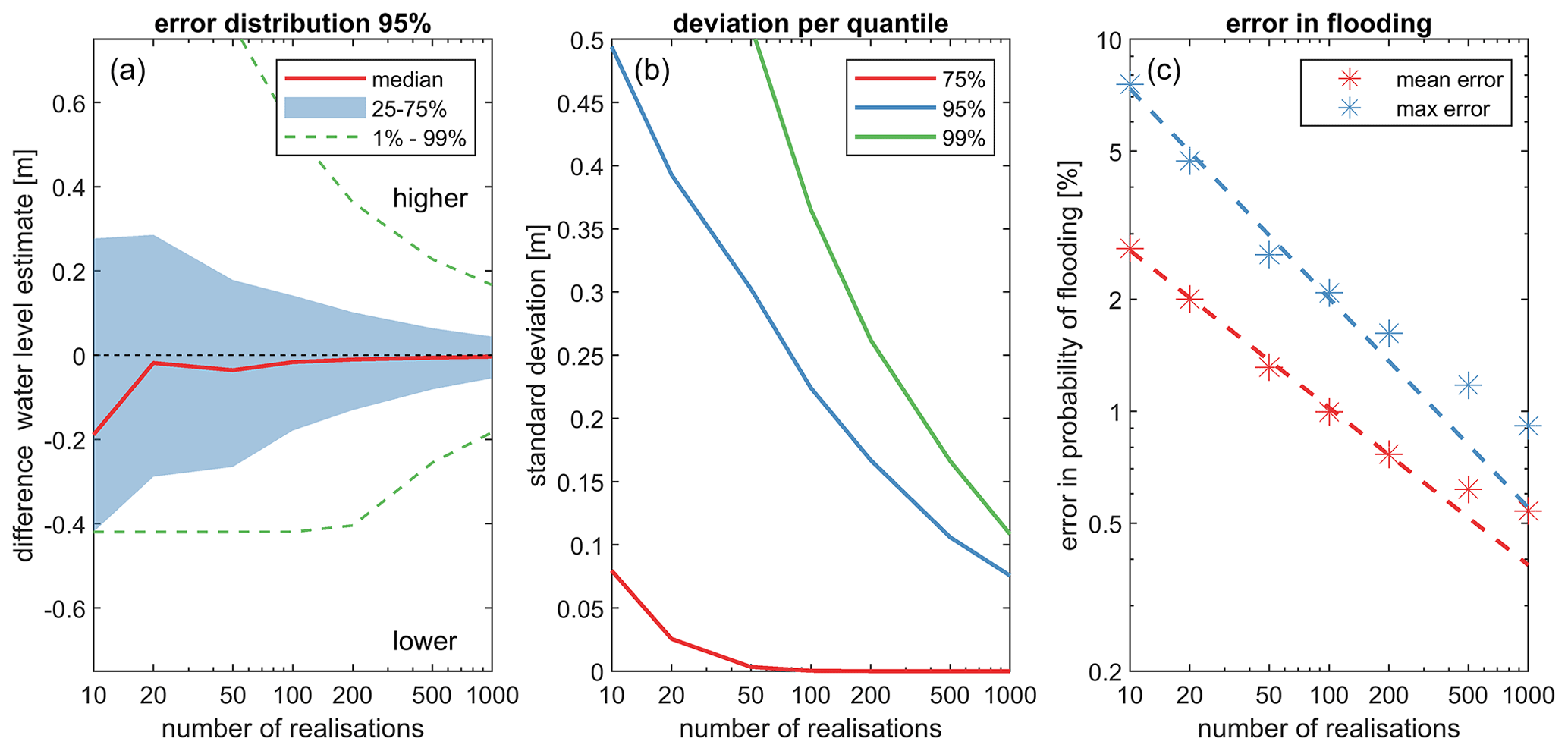
Figure 9 Sampling-size effects on flood estimation accuracy. (a) Quantiles of sampling error for the 5 % exceedance water level. (b) Standard deviation of 75 %, 95 %, and 99 % quantiles, illustrating the uncertainty in estimation. (c) Comparison of maximum and average error in flood probability predictions. All panels were generated using 10 000 ensemble members and a 1000-bootstrap resampling approach. Using more ensemble members reduces the sampling uncertainty.

5.3.3 Importance of lead time

Thus far, the probabilistic TC forecasting framework has been implemented 3 d prior to the landfall of Idai. Nevertheless, the forecast's results fluctuate with lead times, consequently influencing the associated evaluations of water levels (Fig. 10) and flood probabilities (Fig. 11).

The predicted water levels (tide + surge) vary with lead times (Fig. 10a and c). Specifically, at a lead time of 5 d before landfall, a (unsurprisingly) larger spread between the ensemble members is observed compared to lead times of, for example, 1 or 3 d. Moreover, as landfall approaches, the time series converges since increasing ensemble members produces highly similar predictions. For example, notice how individual ensemble members 1 d before landfall show similar storm surges and still-water levels (i.e., the concentration of lines which becomes more apparent in Fig. 10). Moreover, the 5 % and 95 % exceedance values become less spread out and more peaked around landfall (dashed lines in Fig. 10). This convergence is more apparent for the storm surge. The CDF of the maximum storm surge levels increases with reducing lead time (Fig. 10b). For example, the median storm surge increases from 0.5 m 5 d before landfall to 0.9 and 2.0 m for lead times of 3 d and 1 d, respectively (notice the increasing median estimate in the CDF plot from 5 to 1 d in Fig. 10b). This increase in maximum storm surge shows the increasing certainty that the TC will land near Beira. However, for other locations, the opposite may occur as the landfall shifts away from it. The still-water levels are influenced by both tidal motions and the TC (Fig. 11c). This strongly influences the maximum computed still-water level (Fig. 11d). For instance, the lowest maximum water level for all simulations is around ∼ 2 m a.m.s.l., resulting from the maximum tidal range rather than the TC itself. The 95th quantile of the maximum still-water level is 3.4 m a.m.s.l. 5 d prior to landfall, which increases to 3.6 and 4.0 m a.m.s.l. for lead times of 3 d and 1 d, respectively. The best track of Idai is included as a reference and is estimated to have a 9 % probability of exceedance 1 d before landfall.

A large portion of the Sofala Province faces a minor flood risk 5 d before the actual landfall. The flood probability for the estuary near Beira increases as lead times are reduced (Fig. 11b). In particular, the average probability of flooding 5 d before landfall is 15 %, increasing to 17 % and 24 % for lead times of 3 and 1 d, respectively. Conversely, for the entire model domain, a probability of greater than 1 % flooding declines from 97 to 94 and 64 km² for lead times of 5, 3, and 1 d (Fig. 10a). In other words, 5 d before landfall, less confidence in predictions translates into more spatial variability in flooding probability tied to a larger impact area. Closer to the actual landfall, there is more certainty over which area will be affected.

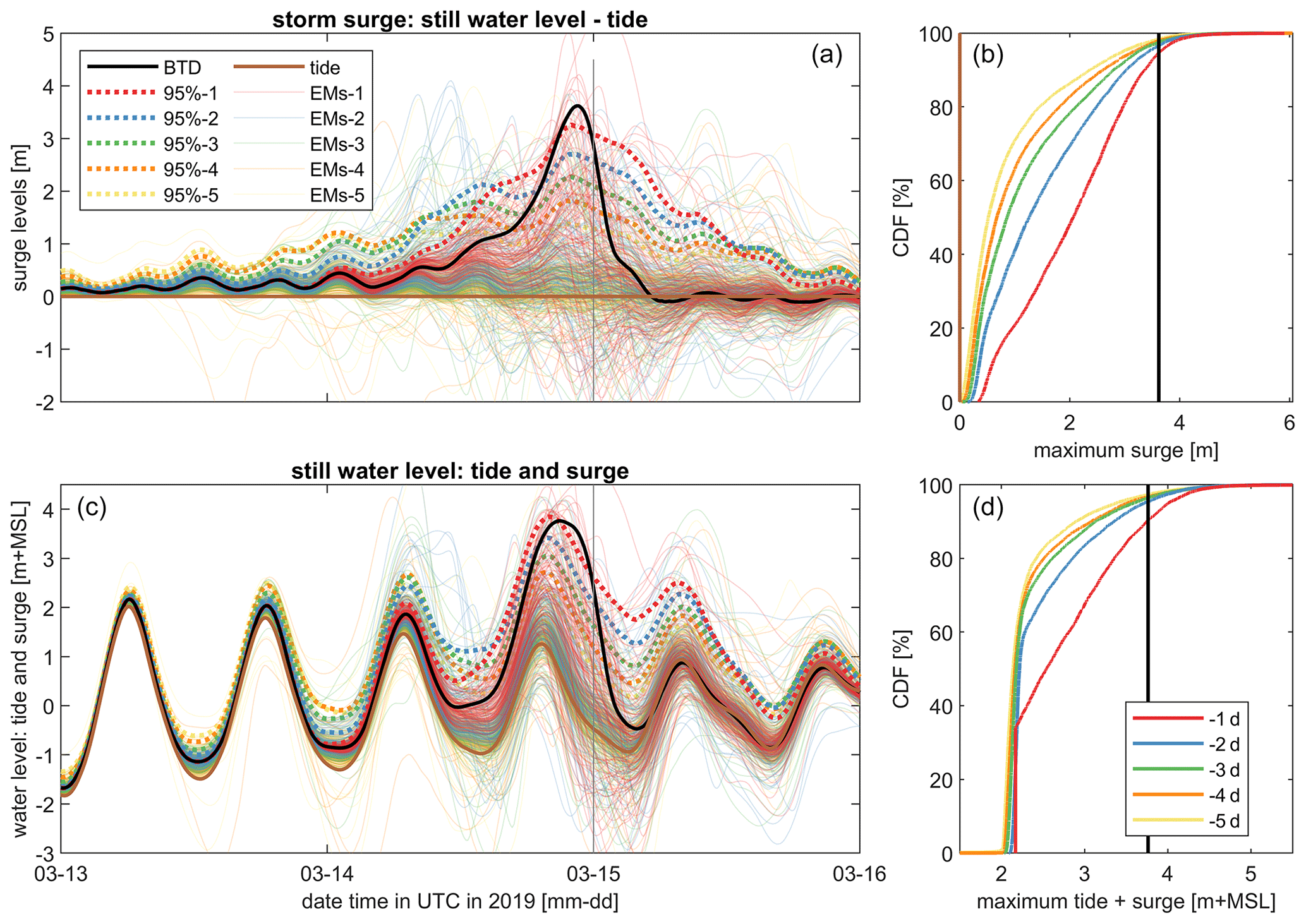
Figure 10 Forecasted water levels in Beira for 1–5 d lead times: temporal evaluation and cumulative distribution. Panels (a) and (c): time series illustrating the forecasted water levels in proximity to Beira with lead times ranging from 1 to 5 d prior to landfall, showcasing both individual ensemble members (solid transparent lines; every 100th plotted) and tide-only (brown), best-track (black), and quantile estimates (95 % dashed lines). Panels (a) and (c) use the same colors and line styles. Panels (b) and (d): cumulative distribution function (CDF) showing the maximum water levels in ascending order for all ensemble members, providing insights into the probability of occurrence for various water level thresholds. Panels (b) and (d) use the same colors. Panels (a) and (b) show the storm surge levels (computed still-water levels minus predicted tidal levels), while panels (c) and (d) present the still-water level (tide and surge).

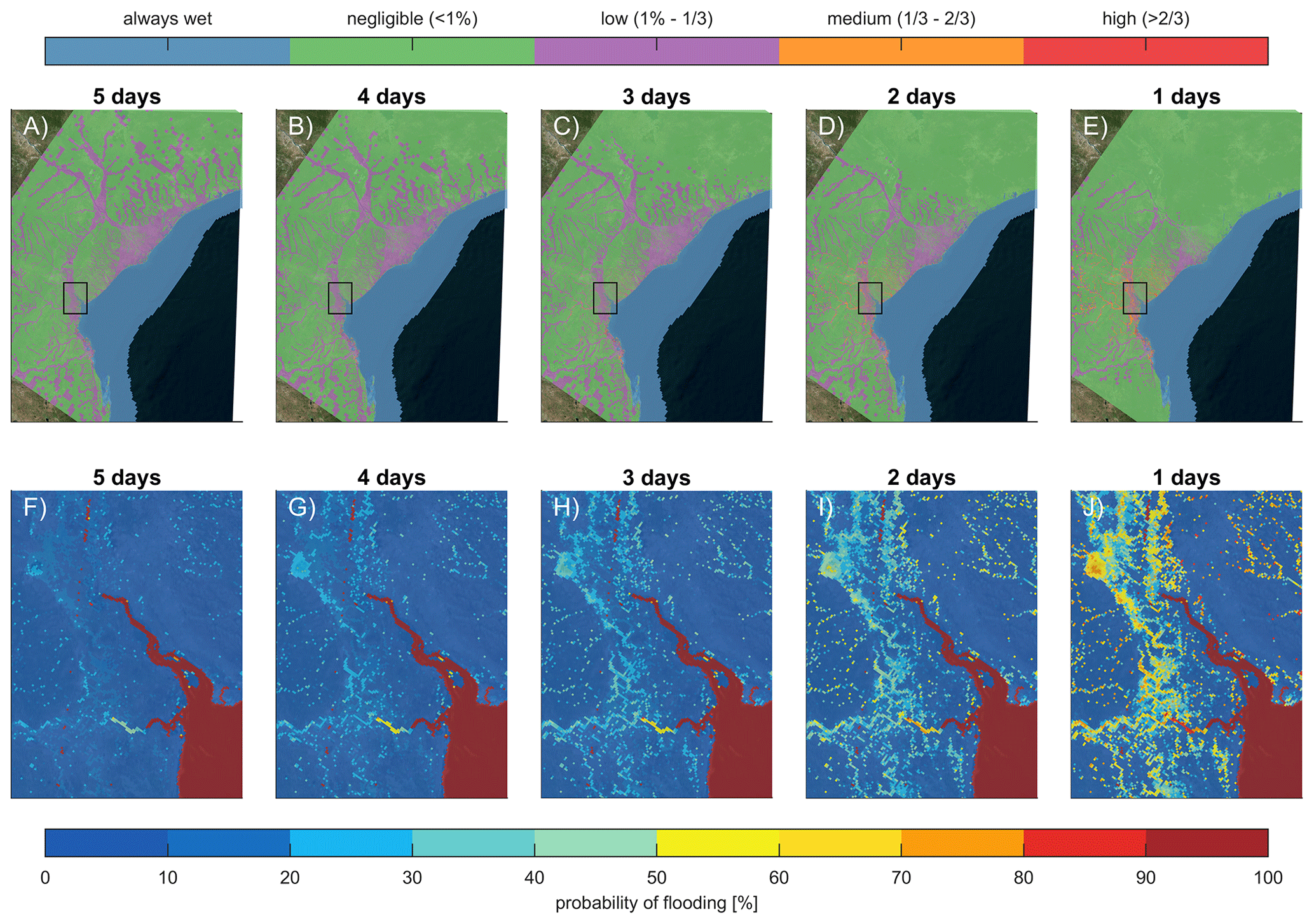
Figure 11 Evolution of the flood probability prior to landfall: panels (a)–(e) depict the spatial distribution of flooding probabilities at 5, 4, 3, 2, and 1 d before landfall, respectively. Color gradients represent the varying probability. The top panels focus on the entire area simulated, and the bottom panels focus on the Pungwe and Buzi river deltas. With decreasing lead times, the area that could be affected decreases, while there is an increased probability of flooding near Beira. The coordinate system of this figure is WGS 84/UTM 36 S (EPSG 32736). © Microsoft.

6 Discussion

This paper describes a new probabilistic method to forecast TC-induced coastal compound flooding by means of tide, surge, and rainfall using Monte Carlo sampling. Due to the limited number of observations on TC evolution, for short-term operational analyses, an autoregressive technique that imposes potential errors on top of the forecasted track is preferred over those parametric sampling techniques used for long-term strategic risk assessments based on historical records (e.g., Nederhoff et al., 2021). In addition, for the same scarcity of observations, there is limited knowledge of the underlying joint distribution between TC and ocean characteristics, which makes Monte Carlo sampling preferred compared to sampling techniques that are highly efficient for complex multivariate patterns such as cluster analysis (e.g., Choi et al., 2009) and MDA methods (e.g., Bakker et al., 2022). However, exploring the possibility of increasing efficiency via the aforementioned methods is important, especially since the error space increases as a function of lead time, and estimating these events requires increasing numbers of ensemble members (Fig. 9b). However, this is a topic that requires an in-depth analysis and is beyond the scope of the present study.

Compared to the implementation of DeMaria et al. (2009) and DeMaria et al. (2013), the ensemble generation is simplified by removing bias corrections, applying a single normal error distribution calibrated on historical errors (Fig. 5), and does not account for the uncertainty of the track forecasts on a case-by-case basis via GPCE. While we acknowledge these simplifications, this method does make it possible to account for TC forecasting errors for any ocean basin based on reported average historical errors alone. Nevertheless, the behavior of a specific tropical cyclone (TC) does not necessarily conform to the “average” pattern, and differences between the operational JTWC model were found (Fig. 6). For Beira, we found minor differences in the comparison of TC-FF and JTWC operational ensembles that do account for the uncertainty of the track forecasts on a case-by-case basis. Thus, the case study presented in this paper suggests that the universal historical error statistics versus a TC-dependent error sampling might be acceptable; however, follow-up work will be needed to test if this finding holds for other TCs. Moreover, the system only accounts for uncertainty in track parameters and does not account for uncertainty in, for example, rainfall or computed storm surge. The implications of these assumptions for the precision and predictive proficiency of our approach for coastal compound flooding remain undetermined. Our implementation has been recently integrated into an operational system tailored for the contiguous United States. Verification of the reliability of this operational system is currently pending. Regardless, TC-FF compares well with the predictions provided by ECMWF of Idai that showed a probability of 50 % to 90 % of severe flooding 4 to 1 d before landfall (Fig. 10). We hypothesize that track uncertainties dominate several days before landfall, while <1 d before, other sources of uncertainty start to become more important and should ideally be accounted for.

In the introduced methodology, we apply the compound-flooding model SFINCS. The validation gave confidence that the hydrodynamic model reproduces the main tidal motions and flooding during Idai. Differences did exist compared to the (limited) validation data (Fig. 4). Additional data sources to assess the model's spatiotemporal accuracy and reliability in simulating the compound-flooding event would be advantageous but were unavailable (at the time this study was performed). The model skill could be improved by including additional wind radii information in the parametric wind model (e.g., radius of gale-force winds along different quadrants) and by more accurately resolving on-land winds, rainfall, and infiltration processes. For example, Done et al. (2020) present a methodology to account for terrain effects by adjusting winds from a parametric wind field model by using a numerical boundary layer model. Here, we applied the IPET empirical relationship that relates pressure drop to rainfall intensity. We chose IPET over other methods since this relatively simple method demonstrated the highest skill in reproducing storm total precipitation in Brackins and Kalyanapu (2020). However, deployment showed the necessity of tripling the rainfall rate due to severe underestimation of the total rainfall and associated flooding. We hypothesize that this does influence model skill from SFINCS but suspect limited influence over results geared towards TC-FF applicability and sensitivity regarding sample size and lead time. Improvement (deterministic or stochastic parametrizations) of TC rainfall could overcome this limitation. For example, we acknowledge that there are other computationally efficient TC rain models in the literature that might perform better (e.g., Lu et al., 2018) and are exploring incorporating these methods in TC-FF. Moreover, SFINCS was run with a constant infiltration rate and does not account for drainage systems, fluvial discharge from the large catchment, and flood protection measures besides the frontal levee. It is also unknown how the topo-bathymetry that was collected before Idai influenced results. Lastly, the effects of waves (e.g., setup, run-up, overtopping) and morphological change were not considered. All these limitations affect the model skill and could explain some mismatches observed compared to Sentinel-1 data and high-water marks at Beira. However, the computational efficiency of SFINCS allowed us to run thousands of ensemble members on limited computational resources. We accept the loss of some model accuracy with this gain in speed. For future developments, we do envision accounting for these uncertainties in addition to variability in track parameters.

The focus of the development of TC-FF has been geared towards the computation of overland flooding. However, TCs pose significant hazards through both water and wind. A study by Rappaport (2014) indicated that, from 1963 to 2012 in the United States, approximately 90 % of fatalities associated with tropical cyclones were due to water-related incidents. The wind-related fatalities were about 8 %. This does not provide insight into the cause of damage associated with landfalling TCs, nor does it provide insight into how these ratios vary across the globe. Regardless, TC-FF does provide the possibility to estimate extreme wind speeds and to link this to potential damage as an additional data product. Including wind damage as part of our framework is something we are planning to work on in the future. Moreover, while this study was written from an operational short-term risk analysis perspective, the same methodology can also be used within strategic long-term risk analysis to explore perturbations to the track and to perform “what if” sensitivity testing with regard to coastal flooding (see, e.g., Rye and Boyd, 2022).

7 Conclusions

A new method and highly flexible open-source tool was developed to perform probabilistic forecasting of tropical-cyclone-induced coastal compound flooding. The Tropical Cyclone Forecasting Framework, TC-FF, computes a set of ensemble members based on a simplified DeMaria et al. (2009) method. In particular, TC-FF uses gridded temporally and spatially varying wind and pressure fields or forecasted tracks and combines this with observed historical along-track, cross-track, and intensity errors. Subsequently, the tool creates a temporally and spatially varying wind field, including rainfall, to force a computationally efficient compound-flood model. This approach allows for the inference of probabilistic wind and flood hazard maps calibrated to any ocean basin in the world with limited computational resources. In contrast to the current practice, TC-FF allows uncertainty analysis using large ensembles produced with physics-based models, narrowing down confidence bands in forecasting coastal compound flooding with a focus on operational TC risk analyses.

The validation of the quadtree SFINCS model for Mozambique's Sofala Province showed reliable skill in terms of tidal propagation in the area of interest (median MAE of 21 cm), including good skill in reproducing the observed flood extent for the case of the flooding caused by Cyclone Idai (2021). The model was able to reproduce the storm surge generation during landfall and flooding near the city of Beira, including the subsequent compound flooding resulting from rainfall runoff in the Pungwe estuary (critical success index of 0.59). Moreover, the model runs efficiently with a wall clock time of 4 minutes for a 7 d event, allowing it to be deployed in probabilistic operational assessments when using multiple cores.

TC-FF was calibrated with the average reported errors for the Southern Hemisphere via the Nelder–Mead method to determine the mean absolute errors and auto-regression coefficients. A comparison between TC-FF and JTWC (based on the complete implementation of DeMaria et al., 2009, and DeMaria et al., 2013) revealed minor differences. In particular, for various lead times from 0 to 120 h, median continuous ranked probability scores (CRPSs) of 0.07, 0.05, and 0.10 and median MAEs of 37 km, 21 km, and 7 m s⁻¹ for, respectively, the along-track, cross-track, and intensity errors were found. These findings give confidence that the TC-FF, including the simplified DeMaria et al. (2009) implementation, can be used for more generalized applications in data-scarce environments.

TC-FF provides valuable insights into the uncertainty of wind speeds, water levels, and potential flooding due to Idai, revealing the impacts of track and intensity uncertainties. This is demonstrated in the wide array of possible maximum wind speeds and significant fluctuations in water levels, which are primarily affected by tidal influences and the cyclone. For instance, even just 3 d prior to landfall, there is a broad spread in the predicted flood areas. This suggests that there is still a significant chance that Idai may not hit the anticipated area or may not generate a substantial storm surge.

The precision of forecasts is directly related to the number of ensemble members used. A mean error in flood probability of less than 1 % and <20 cm sampling errors for the 1 % exceedance water level at Beira required 200 members. Based on that, we determine that at least 200 ensemble members are needed to get reliable water levels and flood results 3 d before landfall. A higher number of ensemble members reduces sampling uncertainty and increases the accuracy of water level and flood potential estimates.

The lead time before landfall has a considerable impact on the forecast's precision. As the lead time decreases, the variability of forecasts diminishes, and the forecasts converge to similar predictions. Similarly, the probability of flooding in certain areas, such as the estuary near Beira, increases as the lead time shortens, providing more certainty over the areas that will be affected by the event.

TC-FF offers a significant advancement compared to the current status quo of a single deterministic simulation when forecasting tropical-cyclone compound-flooding hazards. This approach facilitates a comprehensive understanding of complex interdependencies and uncertainties. By quantifying the likelihood of various outcomes (e.g., by estimating the probability of major flooding in a given neighborhood days before landfall) probabilistic methods enable stakeholders to make more informed decisions and to allocate resources better and enhance preparedness and resilience in the face of these catastrophic natural phenomena.

Appendix A: Tidal calibration and validation

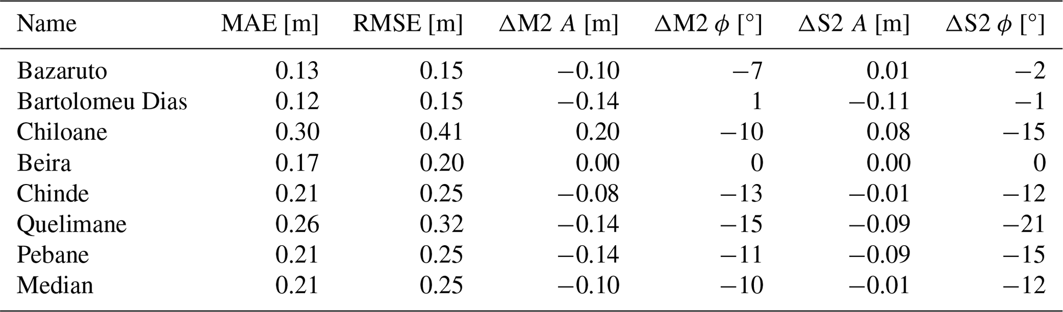
A tidal calibration was performed on the SFINCS-computed tidal constituents compared to the tidal constituents at Beira. Constituents with an amplitude of more than 5 cm (M2, S2, N2, K2, and K1) were adjusted in terms of amplitude (multiplication) and phase (addition). Amplitude changes varied between 0.84 and 1.07, while phase difference changed, on average, by 40°. These calibration steps of adjusting the tidal constituents substantially reduced tidal errors at Beira, specifically reducing the MAE from 43 to 17 cm. Additionally, model skill in reproducing tidal amplitudes and phases is assessed at seven tide stations across the area of interest (including the calibration station of Beira). The SFINCS model reproduces tide with a median MAE of 21 cm, median RMSE of 25 cm, and median differences in M2 and S2 amplitude and phase of, respectively, −10 and −1 cm and −10 to −12° (median values computed over the different stations). Our hypothesis is that the reduction in tidal error observed at Beira throughout the calibration process might be due to a misalignment in the amplitudes and phases of the TPXO model, which were used to generate the tidal boundary conditions (see Sect. 3.1.2). Presumably, the bathymetry contributes to the error observed in the validation process.

Table A1 Evaluation of model proficiency in replicating tides near Sofala Province. Stations are ordered south to north. The first and second columns present the mean absolute error (MAE) and root mean square error (RMSE), respectively, as error metrics for the comparison between observed and simulated tidal time series. The final four columns display the discrepancy (Δ) in amplitude (A) and phase difference (ϕ) for the two most prominent tidal constituents in the area (M2 and S2), where Δ is calculated as the difference between observed and simulated values.

Appendix B: Additional figures for Sect. 5.2.2. (influence of simplifications of TC-FF)

Figures B1, B2, and B3 provide additional information for Sect. 5.2.2. (“Comparison of TC-FF with operational forecast products”).

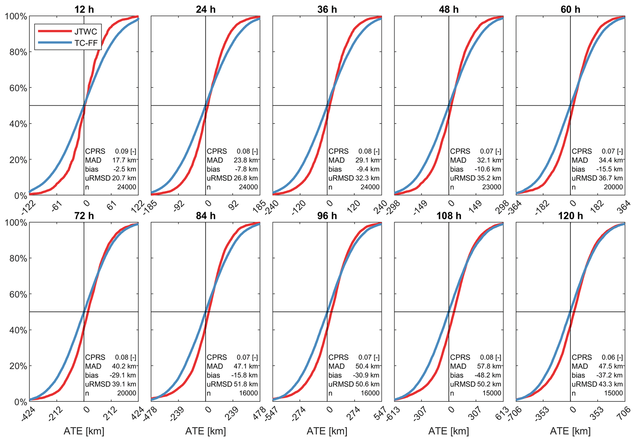
Figure B1 Comparison between the cumulative distribution function (CDF) of the along-track error (ATE) for JTWC (red; reference) and TC-FF (blue; modeled). The different panels represent different lead times.

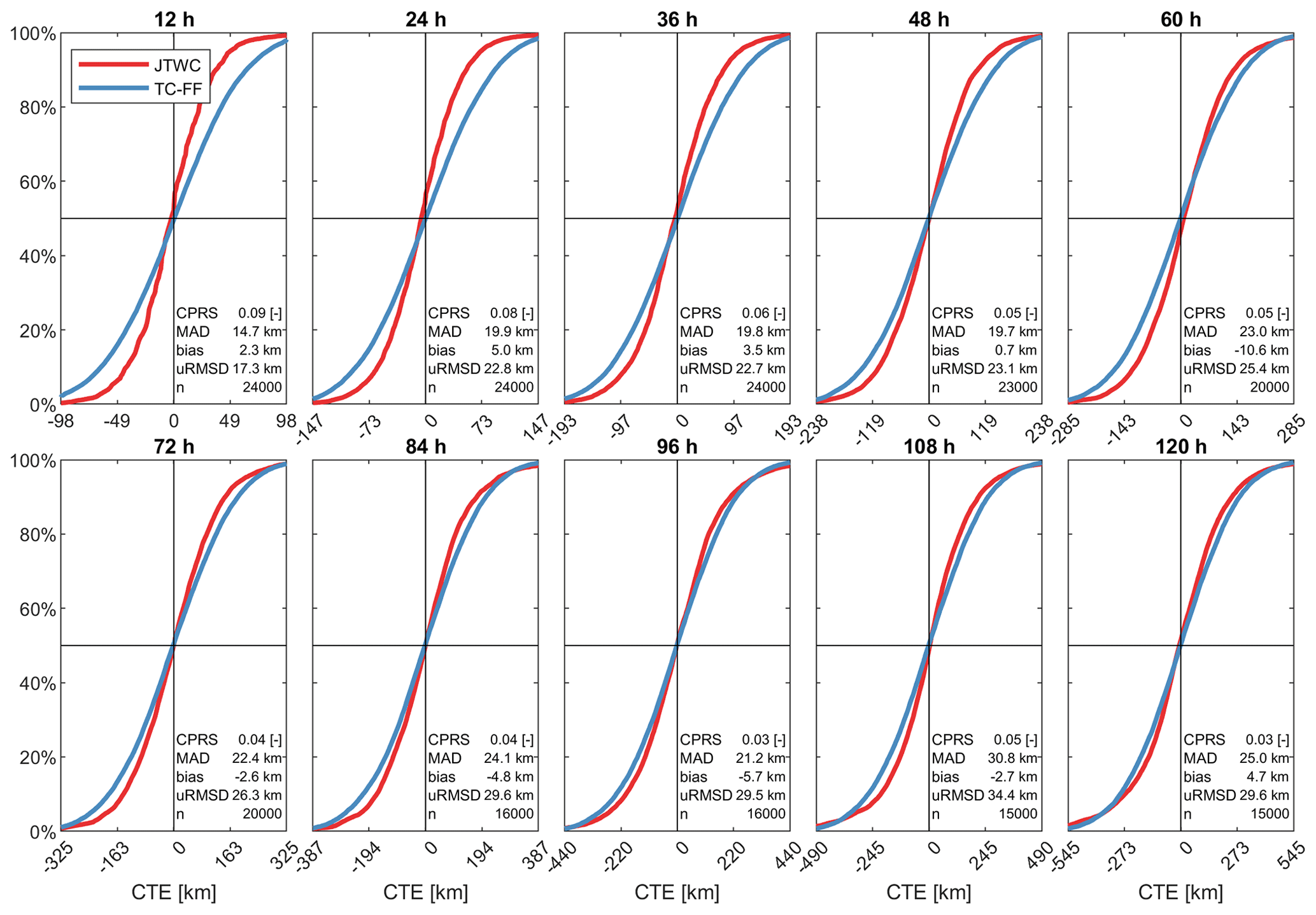
Figure B2 Comparison between the cumulative distribution function (CDF) of the cross-track error (CTE) for JTWC (red; reference) and TC-FF (blue; modeled). The different panels represent different lead times.

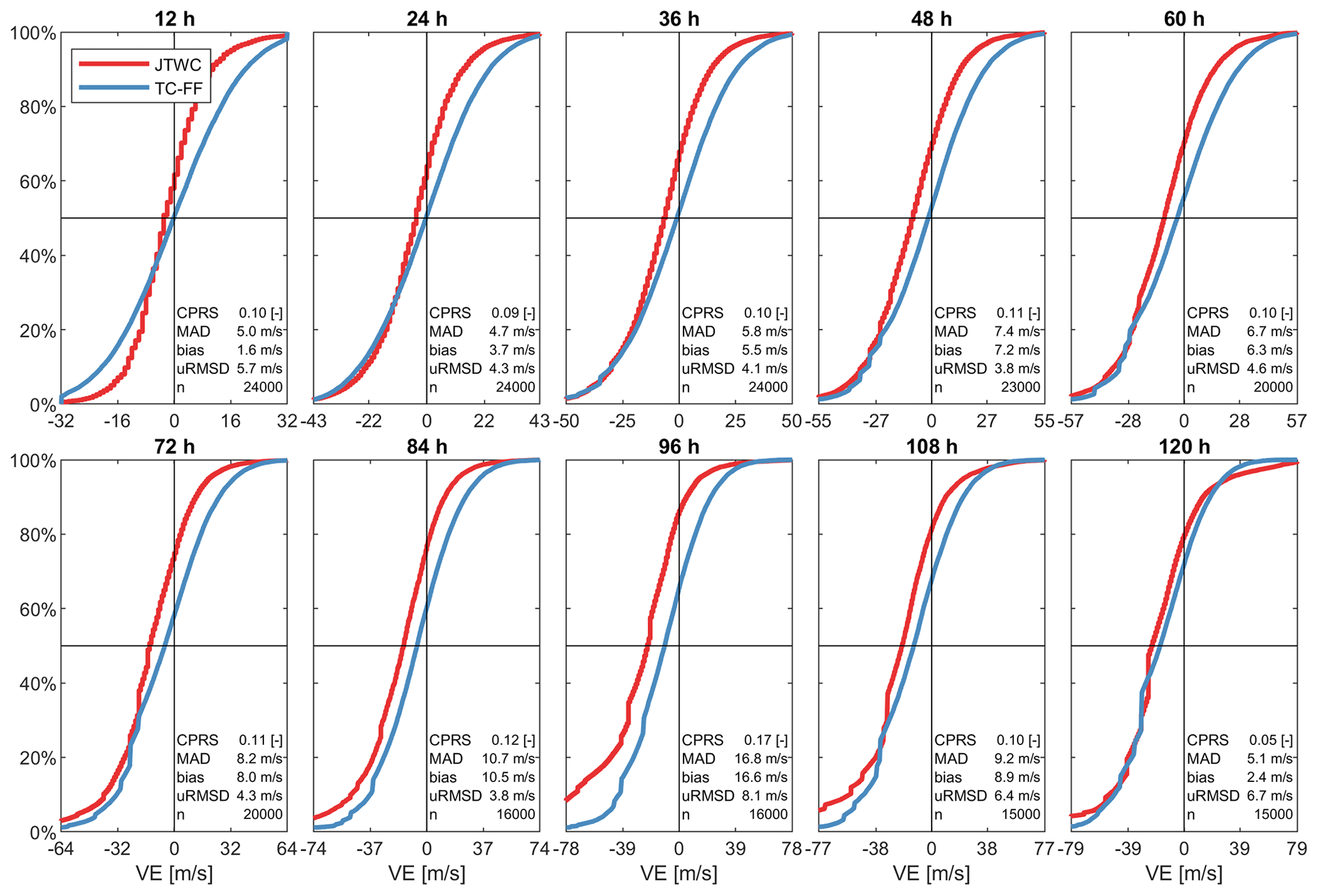
Figure B3 Comparison between the cumulative distribution function (CDF) of the intensity error (VE) for JTWC (red; reference) and TC-FF (blue; modeled). The different panels represent different lead times.